Matched predictions for the $b\bar{b}H$ cross section at the 13 TeV LHC

Abstract

We present up-to-date matched predictions for the $b\bar{b}H$ inclusive cross section at the LHC at $\sqrt{s}=13$ TeV. Using a previously developed method, our predictions consistently combine the complete NLO contributions that are present in the 4-flavor scheme calculation, including finite $b$-quark mass effects as well as top-loop induced $Y_{b}Y_{t}$ interference contributions, with the resummation of collinear logarithms of $m_{b}/m_{H}$ as present in the 5-flavor scheme calculation up to NNLO. We provide a detailed estimate of the perturbative uncertainties of the matched result by examining its dependence on the factorization and renormalization scales, the scale of the Yukawa coupling, and also the low $b$-quark matching scale in the PDFs. We motivate the use of a central renormalization scale of $m_{H}/2$, which is halfway between the values typically chosen in the 4-flavor and 5-flavor scheme calculations. We evaluate the parametric uncertainties due to the PDFs and the $b$-quark mass, and in particular discuss how to systematically disentangle the parametric $m_{b}$ dependence and the unphysical $b$-quark matching scale dependence. Our best prediction for the $b\bar{b}H$ production cross section in the Standard Model at $13$ TeV and for $m_{H}=125\,\mathrm{GeV}$ is $\sigma(b\bar{b}H)=0.52\,{\rm pb}\,\bigl{[}1\pm 9.6\%{\rm(perturbative)}\,{}^{+2.9\%}_{-3.6\%}{\rm(parametric)}\bigr{]}$. We also provide predictions for a range of Higgs masses $m_{H}\in[50,750]\,\mathrm{GeV}$. Our method to compute the matched prediction and to evaluate its uncertainty can be readily applied to other heavy-quark-initiated processes at the LHC.

1 Introduction

Heavy-quark initiated processes and accurate theoretical predictions for them are important for precision tests of the Standard Model (SM), searches for New Physics, and are also essential for the precise determination of parton distribution functions (PDFs).

Predictions for processes involving initial-state $b$-quarks at hadron colliders are typically made using factorization theorems that are valid for two different parametric hierarchies between the $b$-quark mass, $m_{b}$, and the hard-interaction scale of the process, $Q$. In the 4-flavor scheme (4FS), one formally considers $m_{b}\sim Q$, while in the 5-flavor scheme (5FS) one formally considers $m_{b}\ll Q$. The predictions obtained in either scheme have different features. The 4FS predictions include power corrections in $m_{b}/Q$ as well as the exact massive quark final-state phase space, while logarithms of $\ln\left(m_{b}/Q\right)$ are included at a given fixed order. The 5FS predictions do not include power corrections in $m_{b}/Q$ but resum the potentially large logarithms $\ln\left(m_{b}/Q\right)$ to all orders via DGLAP into a $b$-quark PDF. The construction of matched predictions that include the merits of both schemes in DIS (sometimes called variable flavor number schemes) has been the subject of many years of work Aivazis:1993kh ; Aivazis:1993pi ; Thorne:1997ga ; Kretzer:1998ju ; Collins:1998rz ; Cacciari:1998it ; Kramer:2000hn ; Tung:2001mv ; Thorne:2006qt ; Forte:2010ta ; Guzzi:2011ew ; Hoang:2015iva ; Ball:2015dpa and recently progress in this direction for hadron-hadron colliders has also been made Han:2014nja ; Forte:2015hba ; Bonvini:2015pxa .

The focus of this paper is on $b\bar{b}H$ production, for which predictions for the inclusive cross section are available up to NNLO in the 5FS Dicus:1998hs ; Balazs:1998sb ; Harlander:2003ai ; Buehler:2012cu ; Harlander:2012pb and NLO in the 4FS Dittmaier:2003ej ; Dawson:2003kb ; Wiesemann:2014ioa . In the past, the results in the two schemes have been averaged using the pragmatic Santander-Matching prescription Harlander:2011aa . Given that this prescription amounts to a simple weighted average of the two results, it is clear that it does not constitute a satisfactory and theoretically-consistent matching. In particular, as already observed in ref. Bonvini:2015pxa , the contributions present in one and not the other scheme should get added in their combination rather than averaged, which in this case leads to a noticeably higher cross section of the properly matched result compared to the Santander average.

In ref. Bonvini:2015pxa , we used a simple effective field theory setup to systematically derive matched predictions for the $b\bar{b}H$ cross section, which combines the ingredients of both 4FS and 5FS schemes. The result contains the full 4FS result, including the exact dependence on the $b$-quark mass, and improves it with a resummation of collinear logarithms of $m_{b}/m_{H}$, as are present in the 5FS. An important aspect of our construction is the perturbative counting of the effective $b$-quark PDF, which is counted as an $\mathcal{O}(\alpha_{s})$ object for phenomenologically relevant hard (factorization) scales below $\sim 1$ TeV. This counting rearranges the perturbative expansion of the cross section, such that in the massless limit the result corresponds to a reorganized 5FS result. An important advantage is that in this way the logarithms present in the resummed (5FS) result order-by-order exactly match those present in the fixed-order (4FS) contributions. This feature greatly facilitates the combination of both types of contributions.

In this paper, using the approach of ref. Bonvini:2015pxa , we present state-of-the-art predictions for the $b\bar{b}H$ cross section for the LHC at 13 TeV, including a comprehensive study of its perturbative and parametric uncertainties. Our predictions include the effects of top-quark loop-induced interferences, proportional to $Y_{b}Y_{t}$, which are known to be important in the Standard Model Dittmaier:2003ej ; Dawson:2003kb ; Wiesemann:2014ioa . (These were not yet included in ref. Bonvini:2015pxa .) We also investigate in detail the effects of pure 2-loop terms that are present in the 5FS NNLO calculation but are formally of higher order in our perturbative counting.

The two-step matching used in ref. Bonvini:2015pxa makes it explicit that there are two relevant scales in the problem: the hard scale $\mu_{H}\sim m_{H}$ and the $b$-quark scale $\mu_{b}\sim m_{b}$ (also referred to as the $b$-quark threshold scale). Since a perturbative expansion is performed at both of these scales, a reliable theory uncertainty should take into account the perturbative uncertainties related to both. The uncertainty due to $\mu_{b}$ has been neglected in the past in essentially all 5FS and matched cross section predictions, since all standard 5FS PDF sets make the fixed choice $\mu_{b}=m_{b}$. However, the $\mu_{b}$ uncertainty should be regarded as an additional resummation uncertainty, and in ref. Bonvini:2015pxa it was shown how to systematically estimate it and that it can indeed have a nonnegligible effect. We discuss and motivate an appropriate choice of the central scales and provide a full breakdown of theoretical uncertainties due to $\mu_{F}$, $\mu_{R}$, $\mu_{b}$ variations.

We show that this more general setup also disentangles the dependence on $\mu_{b}$ and $m_{b}$ and thus allows one to correctly evaluate the uncertainty in the predictions due to the parametric uncertainty in the value of $m_{b}$. This discussion is relevant for any heavy-quark initiated process calculated in either the fixed 5FS or a matched approach.

The structure of the paper is as follows: in section 2, we recall the main features in the construction of the matched NLO+NLL result and discuss the extensions to include the $Y_{b}Y_{t}$ interference terms and higher-order 2-loop terms. In section 3, we discuss in detail the perturbative and parametric uncertainties. In section 4, we present our numerical results for the inclusive cross section for a range of Higgs masses $m_{H}\in[50,750]\,\mathrm{GeV}$, including the full breakdown of all uncertainties. We conclude and give a short outlook in section 5.

2 Matched cross section

In this section we discuss the theoretical ingredients for our predictions of the $b\bar{b}H$ cross section. In sections 2.1 and 2.2, we summarize the main steps and results of ref. Bonvini:2015pxa in the construction of the fixed-order + resummation matched result, which is valid for any parametric hierarchy between $m_{b}$ and $m_{H}$. For the detailed derivation we refer to ref. Bonvini:2015pxa . In section 2.3, we discuss the inclusion of the formally higher-order two-loop terms in the resummed results. We will denote the corresponding result as NLO+NNLL_partial. In section 2.4, we discuss the inclusion of the $Y_{b}Y_{t}$ interference terms.

2.1 Fixed order and resummed results

The fixed-order cross section that enters the matched result, and which is recovered when the resummation is turned off, is obtained in a factorization scheme that is formally valid for the parametric power counting $m_{b}\sim m_{H}$. Hence, it is equivalent to a 4FS result, where bottom quarks do not appear in the initial-state and can only be produced via gluon splittings into $b$-quark pairs. It includes the exact dependence on the $b$-quark mass (i.e., it includes power corrections to all orders in $m_{b}^{2}/m_{H}^{2}$) both in the partonic cross sections and in the phase space. Logarithmic terms $\sim\ln(m_{b}^{2}/m_{H}^{2})$ arising from collinear gluon splittings are included at fixed order in $\alpha_{s}$. The fixed-order result is given in terms of coefficient functions $D_{ij}(m_{H},m_{b},\mu_{F})$, which depend explicitly on $m_{b}$, and 4-flavor PDFs,

$$\sigma^{\rm FO} =\sum_{i,j=g,q,\bar{q}}D_{ij}(m_{H},m_{b},\mu_{F})\,f^{[4]}_{i}(\mu_{F})\,f^{[4]}_{j}(\mu_{F})$$

$$=\sum_{i,j,k,l=g,q,\bar{q}}D_{ij}(m_{H},m_{b},\mu_{F})\Bigl{[}U^{[4]}_{ik}(\mu_{F},\mu_{0})f^{[4]}_{k}(\mu_{0})\Bigl{]}\Bigr{[}U^{[4]}_{jl}(\mu_{F},\mu_{0})f^{[4]}_{l}(\mu_{0})\Bigr{]}\,.$$ (1)

For notational simplicity, we keep all Mellin convolutions between PDFs, evolution factors, and coefficient functions implicit and simply write products throughout the paper. The sum over partons only includes gluons and light (anti)quarks ($q=d,u,s,c$), $\mu_{F}$ is the hard factorization scale of the process. In the second line the 4-flavor PDFs $f^{[4]}_{j}(\mu_{F})$ are written in terms of the fitted PDFs at the low scale $\mu_{0}$ and DGLAP evolution factors $U^{[4]}_{ij}$ with $n_{f}=4$ active quark flavors. The fixed-order result of eq. (2.1) is equivalent to a 4FS result and the coefficients $D_{ij}$ for $b\bar{b}H$ are known to NLO.

The pure resummed result is based on the factorization theorem derived in the limit $m_{b}\ll m_{H}$, i.e., in a power expansion in $m_{b}/m_{H}$, where the leading power term leads to the usual 5FS result, while subleading power terms correspond to subleading twist terms and are usually not considered. In this case, $b$-quarks are treated as massless at the hard matching scale $\mu_{F}\sim m_{H}$ and appear in the initial state of the corresponding partonic matching calculation. The collinear logarithms of $m_{b}/m_{H}$ are resummed by DGLAP evolution from the hard scale $\mu_{F}\sim m_{H}$ to the $b$-quark matching scale $\mu_{b}\sim m_{b}$. At $\mu_{b}$, the $b$-quark is integrated out of the theory. These steps result in an effective perturbative $b$-quark PDF. The resummed cross section is given by the convolution of coefficient functions $C_{ij}(m_{H},\mu_{F})$, which contain no $m_{b}$ dependence, with 5-flavor PDFs,

$$\sigma^{\rm resum} =\sum_{i,j=g,q,\bar{q},b,\bar{b}}C_{ij}(m_{H},\mu_{F})\,f^{[5]}_{i}(m_{b},\mu_{F})\,f^{[5]}_{j}(m_{b},\mu_{F})$$ (2)

$$=\sum_{i,j=g,q,\bar{q},b,\bar{b}}C_{ij}(m_{H},\mu_{F})\Biggl{[}\sum_{\begin{subarray}{c}k=g,q,\bar{q},b,\bar{b}\\ l,p=g,q,\bar{q}\end{subarray}}U^{[5]}_{ik}(\mu_{F},\mu_{b})\mathcal{M}_{kl}(m_{b},\mu_{b})U^{[4]}_{lp}(\mu_{b},\mu_{0})f^{[4]}_{p}(\mu_{0})\Biggr{]}$$

$$\qquad\qquad\qquad\qquad\qquad\times\Biggl{[}\sum_{\begin{subarray}{c}k=g,q,\bar{q},b,\bar{b}\\ l,p=g,q,\bar{q}\end{subarray}}U^{[5]}_{jk}(\mu_{F},\mu_{b})\mathcal{M}_{kl}(m_{b},\mu_{b})U^{[4]}_{lp}(\mu_{b},\mu_{0})f^{[4]}_{p}(\mu_{0})\Biggr{]}\,.$$

In the second step, the 5-flavor PDFs at $\mu=\mu_{F}$ are written out explicitly in terms of the 5-flavor evolution from $\mu_{F}$ to $\mu_{b}$, the matching at $\mu_{b}$ yielding matching coefficients $\mathcal{M}_{kl}(m_{b},\mu_{b})$ that explicitly depend on $m_{b}$, followed by the 4-flavor evolution from $\mu_{b}$ to $\mu_{0}$ and the fitted 4-flavor PDFs at scale $\mu_{0}$. All mainstream 5FS PDF sets construct their $b$-quark PDFs in this way, however, with the fixed choice of $\mu_{b}=m_{b}$. With this choice, the $\mathcal{O}(\alpha_{s})$ matching coefficients $\mathcal{M}_{ij}$ in the $m_{b}$ pole-scheme are exactly zero, which somewhat simplifies the implementation. However, identifying $\mu_{b}=m_{b}$ confuses the parametric physical dependence on $m_{b}$ and the unphysical dependence on the matching scale $\mu_{b}$, which controls the resummation of logarithms and should cancel to the order one is working. We will discuss how we rectify this situation in section 3.

2.2 Matching fixed order and resummation: NLO+NLL

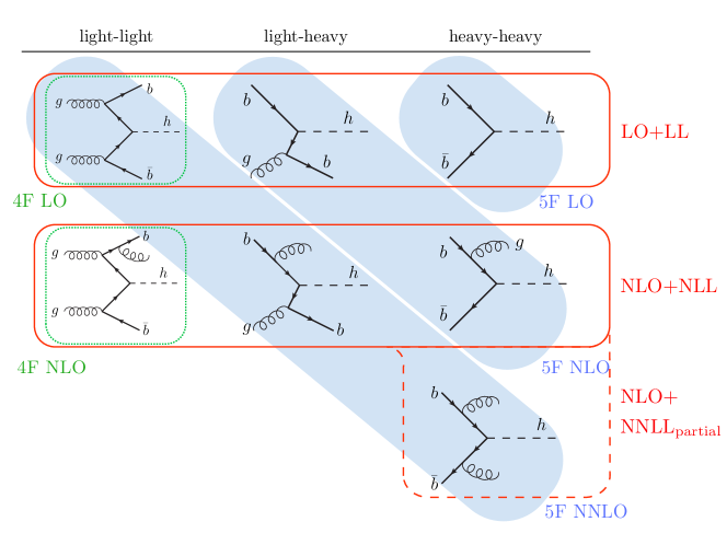
Figure 1: Pictorial representation with sample diagrams appearing in the computation of the $b\bar{b}H$ cross section, grouped according to the different perturbative countings adopted in the 4FS (green boxes), 5FS (blue areas) and our matched resummed result (red boxes).

In all practical applications we are aware of, the evolved PDFs are always treated as external $\mathcal{O}(1)$ objects and the perturbative expansion of the cross section is based solely on the perturbative expansion of the coefficient functions $D_{ij}$ and $C_{ij}$ in eqs. (2.1) and (2). For the fixed-order and resummed results this leads to the usual 4FS and 5FS predictions. The corresponding contributions are schematically depicted in figure 1 by the first column for the 4FS (green dotted boxes) and by the three diagonals (blue shading) for the 5FS.

As noted above, the $b$-quark PDF is itself a perturbative object with the expansion

$$f^{[5]}_{b}(m_{b},\mu_{F}) =\Bigl{[}U_{bg}^{{[5]}}(\mu_{F},\mu_{b})+\frac{\alpha_{s}(\mu_{b})}{4\pi}\,U_{bb}^{{[5]}}(\mu_{F},\mu_{b})\mathcal{M}_{bg}^{(1)}(m_{b},\mu_{b})\Bigr{]}f_{g}^{{[4]}}(\mu_{b})+\,\dotsb$$

$$\sim\qquad\mathcal{O}(\alpha_{s})\quad+\quad\qquad\qquad\qquad\mathcal{O}(\alpha_{s})\qquad\qquad\qquad\qquad+\mathcal{O}(\alpha_{s}^{2})\,.$$ (3)

In principle, each of its terms should be included in the perturbative counting and be regarded as part of the perturbative expansion of the cross section. Counting it as an $\mathcal{O}(1)$ object would be justified in the limit where the off-diagonal evolution factor $U^{[5]}_{bg}(\mu_{F},\mu_{b})\sim 1$. However, $U^{[5]}_{bg}(\mu_{F},\mu_{b})$ is suppressed by an overall $\alpha_{s}\ln(\mu_{F}/\mu_{b})$ relative to the diagonal evolution factors and vanishes in the limit $\mu_{b}\to\mu_{F}$, and therefore this only holds for scales $\mu_{F}\ggg\mu_{b}$. Numerically, for $\mu_{b}\sim m_{b}$ this is only attained for scales $\mu_{F}\gtrsim 1$ TeV. Hence, for the scales of interest here it is more appropriate to count $U^{[5]}_{bg}(\mu_{F},\mu_{b})$ as $\mathcal{O}(\alpha_{s})$, as indicated in eq. (2.2), in which case the whole $f_{b}^{[5]}$ becomes an $\mathcal{O}(\alpha_{s})$ object. The perturbative expansion in $\alpha_{s}$ of the resummed cross section in eq. (2) is then performed by expanding the product of coefficient functions $C_{ij}$ together with the terms making up the $b$-quark PDF including the $b$-quark matching coefficients $\mathcal{M}_{ij}$ and $U_{bg}^{[5]}\sim\alpha_{s}$. For a more detailed discussion we refer to ref. Bonvini:2015pxa .

The 4FS and 5FS results can significantly differ from each other and in particular display different patterns in their factorization-scale dependence due to the different logarithmic terms present at each order in the two schemes. Hence, a consistent matching appears to be nontrivial. The above treatment of the resummed result has the important added advantage that it reorganizes the resummed series into a form that is consistent with the logarithms present in the fixed-order result. The key feature is that order by order in $\alpha_{s}$ the limit $\mu_{b}\to\mu_{F}$ in the resummed cross section now exactly reproduces all the logarithmic terms (and nothing more) that are present in the $m_{b}\to 0$ limit of the fixed-order cross section. In other words, the reexpansion of the resummed result to fixed order is simply given by setting $\mu_{b}=\mu_{F}$. This in turn means that for $\mu_{b}<\mu_{F}$ the evolution factors $U^{[5]}_{ij}$ in this expansion precisely resum the singular logarithms present in the fixed-order result. Hence, all that is missing in the resummed result compared to the fixed-order result are purely nonsingular terms proportional to $m_{b}^{2}/m_{H}^{2}$, i.e. terms that vanish in the limit $m_{b}\to 0$ given by

$$\sigma^{\rm nons}=\sigma^{\rm FO}-\sigma^{\rm resum}\big{|}_{\mu_{b}=\mu_{F}}\,.$$ (4)

The complete matched cross section is then simply given by adding the nonsingular fixed-order terms to the resummed result,

$$\sigma^{\rm FO+resum}=\sigma^{\rm resum}+\sigma^{\rm nons}=\sigma^{\rm resum}+\bigl{(}\sigma^{\rm FO}-\sigma^{\rm resum}\big{|}_{\mu_{b}=\mu_{F}}\bigr{)}\,.$$ (5)

By construction, it satisfies $\sigma^{\rm FO+resum}\to\sigma^{\rm FO}$ in the limit $\mu_{b}\to\mu_{F}$ where the resummation is turned off, as required for a consistently matched prediction. On the other hand, it reduces to $\sigma^{\rm resum}$ in the limit $m_{H}\gg m_{b}$. We emphasize again that this crucially relies on the fact that the nonsingular terms vanish for $m_{b}\to 0$, which in turn relies on adopting the perturbative counting for the resummed result described above. The corresponding terms included in the matched result at each order are depicted by the rows (red boxes) in figure 1.

As discussed in ref. Bonvini:2015pxa , for the practical implementation, the nonsingular contributions can be conveniently absorbed into modified gluon and light-quark coefficient functions, $\bar{C}_{ij}(m_{H},m_{b},\mu_{F})$, which now carry an explicit dependence on $m_{b}$, convolved with effective 5F PDFs. The final matched result is then written as

$$\sigma^{\rm FO+resum} =\sum_{i,j=b,\bar{b}}C_{ij}(m_{H},\mu_{F})\,f^{[5]}_{i}(m_{b},\mu_{F})\,f^{[5]}_{j}(m_{b},\mu_{F})$$

$$\quad+\sum_{\begin{subarray}{c}i=b,\bar{b}\\ j=g,q,\bar{q}\end{subarray}}\Bigl{[}C_{ij}(m_{H},\mu_{F})\,f^{[5]}_{i}(m_{b},\mu_{F})\,f^{[5]}_{j}(m_{b},\mu_{F})+(i\leftrightarrow j)\Bigr{]}$$

$$\quad+\sum_{i,j=g,q,\bar{q}}\bar{C}_{ij}(m_{H},m_{b},\mu_{F})\,f^{[5]}_{i}(m_{b},\mu_{F})\,f^{[5]}_{j}(m_{b},\mu_{F})\,,$$ (6)

where $f^{[5]}_{i,b}$ are perturbative objects, and an expansion of $C_{ij}$ and $\bar{C}_{ij}$ against $f^{[5]}_{i,b}$ as discussed above is implicit.

The strict expansion of the coefficient functions against the individual terms making up the $b$-quark PDF is quite inconvenient for the practical implementation, as it requires performing the entire $n_{f}=5$ DGLAP evolution above $\mu_{b}$ by hand. However, as long as we are only interested in the phenomenologically relevant region $\mu_{b}\sim m_{b}\ll\mu_{F}\sim m_{H}$, we can also keep formally higher-order cross terms in order to simplify the practical implementation. Doing so allows us to use common preevolved 5FS PDFs, under the condition that we count $f^{[5]}_{b}\sim\mathcal{O}(\alpha_{s})$ while the light quark and gluon PDFs are counted as $\sim\mathcal{O}(1)$. In addition, we have to use PDFs of sufficiently high order such that they include all matching corrections required by our perturbative counting. Specifically, at (N)LO+(N)LL this requires the use of at least (N)NLO PDFs. It was explicitly checked in ref. Bonvini:2015pxa that for values of $m_{b}/m_{H}\lesssim 0.1$ this implementation gives practically the same numerical results as the strict expansion. On the other hand, the strict expansion is required if one wishes to explicitly study the limit $\mu_{b}\to\mu_{F}$ and obtain a smooth transition of the matched result into the fixed-order result.

In summary, with this simplification, expanding the matched cross section in powers of $\alpha_{s}=\alpha_{s}(\mu_{F})$, the following perturbative expansion is obtained

LO+LL $$\sigma =\quad\alpha_{s}^{2}\bar{C}^{(2)}_{ij}\,f_{i}^{[5]}f_{j}^{[5]}+\alpha_{s}4C^{(1)}_{bg}\,f_{b}^{[5]}f_{g}^{[5]}+\phantom{\alpha_{s}}2C^{(0)}_{b\bar{b}}\,f_{b}^{[5]}f_{b}^{[5]}$$

NLO+NLL $$\quad+\alpha_{s}^{3}\bar{C}^{(3)}_{ij}\,f_{i}^{[5]}f_{j}^{[5]}+\alpha_{s}^{2}4C^{(2)}_{bk}\,f_{b}^{[5]}f_{k}^{[5]}+\alpha_{s}2C^{(1)}_{b\bar{b}}\,f_{b}^{[5]}f_{b}^{[5]}$$

NNLO+NNLL $$\quad+\alpha_{s}^{4}\bar{C}^{(4)}_{ij}\,f_{i}^{[5]}f_{j}^{[5]}+\alpha_{s}^{3}4C^{(3)}_{bk}\,f_{b}^{[5]}f_{k}^{[5]}+\alpha_{s}^{2}(2C^{(2)}_{b\bar{b}}+2C^{(2)}_{bb})\,f_{b}^{[5]}f_{b}^{[5]}$$

$$\quad+\mathcal{O}(\alpha_{s}^{5})\,.$$ (7)

The factors of two and four account for the exchange of partons among the two protons and (to a first approximation) the equality $f_{b}^{[5]}=f_{\bar{b}}^{[5]}$. A sum over light quarks and gluons is implicitly assumed for repeated indices $i,j,k$. The superscripts on the coefficient functions indicate the order in $\alpha_{s}$ to which these are computed. The first two orders in eq. (2.2) are illustrated by the red boxes in figure 1. As seen there, our perturbative counting implies that we include $b\bar{b}$, $bg$ and $gg$ initiated contribution consistently at the same order.

Finally, we note that the construction of the coefficient functions $\bar{C}_{ij}$ is formally the same as the corresponding construction in the FONLL approach Forte:2015hba (and in a hypothetical S-ACOT construction). There are, however, two main differences between these approaches. First, as explained above, we use the fact that the effective $b$-quark PDF counts as an $\mathcal{O}(\alpha_{s})$ perturbative object to construct the perturbative expansion of our matched result. As a result, it contains the complete fixed-order result at each perturbative order, and (with the strict expansion) smoothly merges into it. Secondly, as discussed further in section 3, in our approach we explicitly distinguish $\mu_{b}$ and $m_{b}$ allowing us to include an explicit estimate of the resummation uncertainty associated with the 5F resummation by varying the (in principle arbitrary) matching scale $\mu_{b}$.

2.3 Higher-order two-loop terms: NLO+NNLL_partial

At present, all coefficient functions in eq. (2.2) required up to NLO+NLL are known Harlander:2003ai ; Buehler:2012cu ; Dittmaier:2003ej ; Dawson:2003kb . Going to NNLO+NNLL is not yet possible and would require the full NNLO 4FS result, corresponding to the unknown $\bar{C}^{(4)}_{ij}$ and $C^{(3)}_{bk}$ coefficients in eq. (2.2), together with the three-loop matching coefficients $\mathcal{M}_{ij}$. The two-loop coefficients $C^{(2)}_{b\bar{b}}$ and $C^{(2)}_{bb}$ are known from the NNLO 5FS result Harlander:2003ai and are part of the NNLL resummation in our counting. Adding them to the NLO+NLL result provides a partial NNLL result, see figure 1, which we denote as NLO+NNLL_partial. (In ref. Bonvini:2015pxa , this result was called NLO+NLL+$C^{(2)}_{b\bar{b}}$. It corresponds to what in ref. Forte:2015hba would be called FONLL-B.)

Including the partial NNLL terms violates the exact correspondence between the resummed and fixed-order results. That is, the fixed-order limit of these resummed terms are only reproduced by the $m_{b}\to 0$ limit of the fixed-order result at NNLO. Hence, in the limit $\mu_{b}\to\mu_{F}$ these terms spoil the smooth matching of the matched result into the fixed-order result. In this regard, these terms are analogous to the higher-order cross terms that are kept when the strict expansion is not implemented. Therefore, whenever the strict expansion is used these terms should also be consistently dropped. This is the case when going toward larger values of $m_{b}/m_{H}$, where the logarithms become small and fixed-order contributions become dominant, and the matched result is transitioning into the pure fixed-order result.

For intermediate values of $m_{H}$ (small values of $m_{b}/m_{H}$) where our perturbative counting is most appropriate, including these terms does not necessarily improve the overall accuracy of the prediction, since other terms of the same perturbative order are not included and including only a partial set of terms might bias the result in the wrong direction. At the same time, their inclusion can lead to a reduced scale dependence, which would then potentially underestimate the perturbative uncertainties. For these reasons, we do not take the NLO+NNLL_partial prediction to be our default result. Nevertheless, we also provide it in section 4, as it can provide an indication of the numerical size of the next-order correction. This can for example be an additional useful cross check on the estimate of the perturbative uncertainties of the NLO+NLL result or alternatively guide the choice of the central scales.

Finally, in the limit of very large $m_{H}$ (very small values of $m_{b}/m_{H}$), including these terms becomes beneficial once the size of the resummed logarithms grows, $\alpha_{s}\ln(\mu_{F}^{2}/\mu_{b}^{2})\sim 1$, and the original strict 5FS counting applies.

2.4 Fixed-order nonsingular $Y_{b}Y_{t}$ contributions

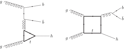
Figure 2: Sample 1-loop diagrams contributing to the $Y_{b}Y_{t}$ interference contribution at fixed order.

At LO there is only a contribution proportional to $Y^{2}_{b}$. Starting at NLO, the cross section receives contributions proportional to $Y_{b}Y_{t}$ due to the interference of the Born-level $gg\to b\bar{b}H$ diagrams with diagrams where the Higgs is radiated from a closed top-quark loop; some examples of the latter diagrams are shown in figure 2. The fixed-order (4FS) cross section can be written schematically as

$$\sigma^{\rm FO} =\alpha_{s}^{2}\,Y_{b}^{2}\,\sigma^{(0)}+\alpha_{s}^{3}\Bigl{(}Y_{b}^{2}\,\sigma^{(1)}_{Y_{b}^{2}}+Y_{b}Y_{t}\,\sigma^{(1)}_{Y_{b}Y_{t}}\Bigr{)}+\mathcal{O}(\alpha_{s}^{4})\,,$$ (8)

where the interference terms are included in $\sigma^{(1)}_{Y_{b}Y_{t}}$.

These top-loop diagrams have the same structure as the contributions that enter the $gg\to H$ gluon-fusion cross section, so the $Y_{b}Y_{t}$ interference contributions fundamentally correspond to an interference between the $b\bar{b}H$ and gluon-fusion processes. Since they involve $b$-quarks in the final state, they are usually regarded as part of the $b\bar{b}H$ cross section.

Curiously, these terms can be treated as purely nonsingular terms, even though they may, at first sight, appear to contain large logarithms of $m_{b}/m_{H}$ in the $m_{b}\to 0$ limit. On closer inspection, these interference terms turn out to vanish to all orders in the $m_{b}\to 0$. The reason is that in the interference between $b\bar{b}H$-like and gluon-fusion-like diagrams the Higgs boson must be attached to two different closed fermion lines. This requires a helicity flip on the $b$-quark line, which is not allowed for $m_{b}=0$. Equivalently, for $m_{b}=0$, they will always contains a trace over an odd number of Dirac matrices and thus vanish Harlander:2003ai . For the same reason, such terms are absent in the 5FS.

For us, this means that these terms are purely nonsingular and can be straightforwardly added by including them in $\sigma^{\rm FO}$ in eq. (8), which then enters into the $\bar{C}^{(3)}_{ij}$ in eq. (2.2). In practice, we extract the numerical result for $\sigma^{(1)}_{Y_{b}^{2}}$ and $\sigma^{(1)}_{Y_{b}Y_{t}}$ in the pole scheme from Madgraph5_aMC@NLO Alwall:2014hca by generating the process $pp\to b\bar{b}H$ at NLO with $Y_{t}$ turned on and off. These are then used to construct $\bar{C}^{(3)}_{ij}$ in the $\overline{\rm MS}$ scheme for the Yukawa couplings.

The $Y_{b}Y_{t}$ interference terms have a noticeable numerical effect ($\sim 5\%$) in the SM, while in beyond-the-Standard-Model (BSM) scenarios such as SUSY with large $\tan\beta$ their relative effect compared to the dominant $Y_{b}^{2}$ contribution tends to be much milder. In section 4 we therefore provide the results both with and without the $Y_{b}Y_{t}$ terms included, which we denote as NLO[$Y_{b}^{2}$] and NLO[$Y_{b}^{2}\!+\!Y_{b}Y_{t}$] in the following. For our choice of central scales, the $Y_{b}Y_{t}$ terms reduce the cross section for $m_{H}\lesssim 300$ GeV and increase it for $m_{H}\gtrsim 300$ GeV, see figure 4 below.

3 Estimate of perturbative and parametric uncertainties

We now turn to the discussion of the theoretical and parametric uncertainties. The estimation of the perturbative uncertainties by variations of the hard scales $\mu_{F}$ and $\mu_{R}$, and low matching scale $\mu_{b}$ are discussed in section 3.1. The parametric uncertainty from the value of the $b$-quark mass is discussed in section 3.2. In section 3.3, we discuss the PDF uncertainty and the construction of modified PDF sets that are required to properly separate the $m_{b}$ and $\mu_{b}$ uncertainties.

3.1 Scale choices and perturbative uncertainties

As discussed in detail in ref. Bonvini:2015pxa , we can distinguish two different sources of perturbative uncertainties. One is an overall “fixed-order” uncertainty (within the resummed or matched results), which can be estimated by exploiting the dependence on the hard matching scale. The second is a “resummation” uncertainty related to the uncertainty in the resummed logarithmic series, which can be estimated by exploiting the dependence on the low $\mu_{b}$ matching scale.

In ref. Bonvini:2015pxa we considered a common hard scale. Here, we additionally study the dependence of the cross section on the renormalization scale $\mu_{R}$ at which $\alpha_{s}$ is evaluated and on the renormalization scale $\mu_{Y}$ at which the Yukawa coupling is evaluated. In this case, the role of the hard matching scale in the resummation is played by the factorization scale $\mu_{F}$ at which the PDFs are evaluated.

3.1.1 Central scale choices

For the factorization scale $\mu_{F}$ we use the central choice $\mu_{F}=(m_{H}+2m_{b})/4$, as is commonly used in both the 4FS and 5FS calculations. This choice is motivated by the well-known observation that in $b\bar{b}H$ such a small factorization scale leads to an improved perturbative convergence, see e.g. Maltoni:2003pn ; Maltoni:2005wd ; Maltoni:2012pa ; Bonvini:2015pxa ; Harlander:2015xur . We point out that the matched NLO+NLL result turns out to be significantly less sensitive to the central value of $\mu_{F}$ Bonvini:2015pxa than the 4FS and 5FS results. The value of $m_{b}$ in the definition of $\mu_{F}$ is taken to be the central pole mass value $m_{b}=4.58$ GeV (see section 3.2), and is kept fixed under $m_{b}$ variations.

For the renormalization scale we use a somewhat larger central value $\mu_{R}=m_{H}/2$. This is motivated by the fact that kinematical arguments for a small scale $\sim m_{H}/4$ are related to the collinear factorization ($\mu_{F}$) and not the renormalization ($\mu_{R}$). On the other hand, choosing $\mu_{R}=m_{H}$, which would be the canonical renormalization scale, produces somewhat artificial leftover $\ln(\mu_{R}/\mu_{F})\simeq\ln 4$ terms in the cross section, which become even larger under scale variations. The value $\mu_{R}=m_{H}/2$ is a reasonable compromise that lies halfway between the standard 4FS and 5FS choices of $\mu_{R}=(m_{H}+2m_{b})/4$ and $\mu_{R}=m_{H}$. Also, at the Higgs masses of interest, the matched result is dominated by the resummation contributions and as shown in ref. Harlander:2015xur the 5FS tends to favor $\mu_{R}$ values between $m_{H}/2$ and $m_{H}$. Finally, this choice has the convenient side effect that the NLO+NNLL_partial result turns out to be a very small correction over the NLO+NLL result.

The Yukawa couplings $Y_{b}(\mu_{Y})$ and $Y_{t}(\mu_{Y})$ are defined in the $\overline{\rm MS}$ scheme are obtained by evolving from $\overline{m}_{b}(\overline{m}_{b})=4.18\,\mathrm{GeV}$ Agashe:2014kda and $\overline{m}_{t}(\overline{m}_{t})=162.7\,\mathrm{GeV}$ Denner:2047636 to the central Yukawa scale $\mu_{Y}$ with 4-loop evolution, while $\mu_{Y}$ variations are computed using 2-loop evolution. While both $\mu_{R}$ and $\mu_{Y}$ are renormalization scales, they do not necessarily need to be the same. It is always possible to evolve $\alpha_{s}$ and the Yukawa coupling to different scales using their own renormalization group evolution, compensated by including the appropriate fixed-order logarithms in the partonic coefficients. In figure 3 we study the dependence of the cross section on $\mu_{R}$ and $\mu_{Y}$ at different orders, always keeping $\mu_{F}$ fixed at its central value. We find that varying $\mu_{R}$ and $\mu_{Y}$ together gives the largest scale variation, so for our numerical results and uncertainty estimation we identify $\mu_{Y}\equiv\mu_{R}$ as is usually done. We also observe that at LO+LL and NLO[$Y_{b}^{2}$]+NLL the renormalization scale dependence comes entirely from the $\mu_{Y}$ dependence, which reduces significantly at each higher order. (This is also another motivation to choose a higher central scale for $\mu_{R}$ since $m_{H}$ is the (only) relevant scale seen by the $b\bar{b}H$ vertex.) Note that at NLO[$Y_{b}^{2}$]+NNLL_partial the $\mu_{Y}$ dependence reduces, which is precisely to be expected from the included two-loop virtual corrections. On the other hand, the $\mu_{R}$ dependence for fixed $\mu_{Y}$ at NLO[$Y_{b}^{2}$]+NNLL_partial actually increases, which could well be related to only including a partial set of higher-order terms.

We note that this observed pattern for the $\mu$ dependence is somewhat changed by the inclusion of the $Y_{b}Y_{t}$ interference terms. This is not unexpected, since these terms introduce new LO dependence on both $\mu_{R}$ and $\mu_{Y}$. However, since their absolute correction to the cross section is small, we base our discussion of the scale choices on the pattern observed without interference terms.

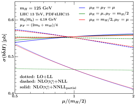
Figure 3: Dependence of the cross sections on $\mu_{R}$ and $\mu_{Y}$ at LO$+$LL (dotted), NLO[$Y_{b}^{2}$]$+$NLL (dashed), and NLO[$Y_{b}^{2}$]$+$NNLL_partial (solid) for $m_{H}=125$ GeV and 13 TeV. The blue curves show the total scale dependence when setting $\mu_{R}=\mu_{Y}=\mu$, the green curves show the dependence on $\mu_{R}=\mu$ for fixed $\mu_{Y}=m_{H}/2$, and the red curves show the dependence on $\mu_{Y}=\mu$ for fixed $\mu_{R}=m_{H}/2$. In call cases $\mu_{F}$ is held fixed at its central value.

Finally, for $\mu_{b}$ we take the canonical central value $\mu_{b}=4.58\,\mathrm{GeV}$, which corresponds to the central pole mass value we use, but importantly is kept fixed under $m_{b}$ variations. The canonical scale choice $\mu_{b}=m_{b}$ is appropriate in the resummation region where $\mu_{b}\ll\mu_{F}$, which is the case for all Higgs masses we consider in this paper. As explained in ref. Bonvini:2015pxa , for larger values of $m_{b}/\mu_{F}\gtrsim 0.3$ (smaller $m_{H}$) one enters the transition region, where the strict expansion should be used and $\mu_{b}$ should be chosen via a more general profile scale to allow for a smooth turning off the resummation and transition into the fixed-order limit $m_{b}\sim\mu_{F}$.

3.1.2 Estimate of perturbative uncertainties

In ref. Bonvini:2015pxa , $\mu_{R}=\mu_{Y}=\mu_{F}$ were all varied together, which already yields an excellent perturbative convergence. Here we follow an even more conservative approach and also explore independent variations of $\mu_{R}$ and $\mu_{F}$. We consider the usual 7-point variation where the two scales are varied independently up and down by factors of two, excluding the two cases where they are both varied in opposite directions. Whenever varying $\mu_{F}$ up or down, the low matching scale $\mu_{b}$ is varied up or down by the same factor, such that the ratio $\mu_{F}/\mu_{b}$ and therefore the resummed logarithms remain fixed. As discussed in ref. Bonvini:2015pxa , this allows us to interpret the hard scale variations as an estimate of the overall fixed-order uncertainty. The final fixed-order uncertainty is then obtained by the maximal envelope, i.e., we use the absolute value of the largest deviation from the central value as the symmetric uncertainty. Doing so explicitly avoids attributing any physical meaning to accidentally small one-sided scale dependence (that would yield asymmetric uncertainties), which just results from a nonlinear scale dependence as frequently encountered at higher orders or near the points of minimal scale dependence.

Next, the resummation uncertainty is computed by varying the matching scale $\mu_{b}$ by a factor of 2 up and down about its central value. For this variation we keep all the other scales fixed (and also the value of $m_{b}$). Doing so explicitly changes the ratio $\mu_{F}/\mu_{b}$ and thus directly probes the size of the resummed logarithms.

The fixed-order and resummation uncertainties are considered as independent uncertainty sources, and the total perturbative uncertainty is obtained by adding them in quadrature. A simple alternative approach, which however lacks the physical interpretation of the source of uncertainty, would be to consider all possible independent variations of $\mu_{F}$, $\mu_{R}$, $\mu_{b}$ by factors of two, eliminating all cases where the ratio of any two variation factors exceeds $2$, and taking the total envelope. This turns out to be more aggressive and produces a smaller total uncertainty, because some of the variations (the $\mu_{b}$ variations in particular) that in our approach are considered independent and added in quadrature, are simply contained within the overall envelope and thus have no effect on the final uncertainty.

3.2 Parametric uncertainties due to $m_{b}$

We now discuss the settings we use for the $b$-quark mass. The $b$-quark mass is most precisely measured when defined in a renormalon-free short-distance scheme, such as the $\overline{\rm MS}$ or $1S$ schemes. As our starting point and central input value we thus take the measured value of the $\overline{\rm MS}$ mass $\overline{m}_{b}(\overline{m}_{b})=4.18\pm 0.03$ GeV Agashe:2014kda .

In principle, the best option would be to always use a renormalon-free mass renormalization scheme along with the corresponding measured value in all the places where the mass appears. These are the Yukawa coupling $Y_{b}$, the $m_{b}$ dependence in the nonsingular parts of the coefficient functions, and the $m_{b}$ dependence of the PDF matching coefficients $\mathcal{M}_{ij}(m_{b},\mu_{b})$ [see eq. (2)]. As mentioned in section 3.1 above, the Yukawa coupling is renormalized in the $\overline{\rm MS}$ scheme and is directly obtained by evolving from $\mu=\overline{m}_{b}$ to $\mu_{R}$.

Unfortunately, most current PDF fits are performed with pole-scheme masses, including all PDF sets that currently enter the PDF4LHC15 combination, which is what we will utilize, see section 3.3 below. Furthermore, the fixed-order computations that we use as input and hence our nonsingular coefficient functions are currently obtained in the pole scheme. To be consistent, we thus also require $m_{b}$ in the pole scheme.

Since the pole mass has a leading renormalon ambiguity, the choice of its value is somewhat delicate. To reproduce as closely as possible the renormalon cancellation that would happen when properly translating the perturbative expressions from the pole scheme to the $\overline{\rm MS}$ scheme, we have to convert the $\overline{m}_{b}$ input value to a pole-mass value at the same loop order at which the perturbative series where $m_{b}$ appears (and that contains the cancelling renormalon) is used. In our case, this means we should translate it at 1-loop order because the proper NLO+NLL $\overline{\rm MS}$ result would require an NNLO $\overline{\rm MS}$ PDF set and would be affected by the 1-loop pole to $\overline{\rm MS}$ conversion,

$$\overline{m}_{b}(\overline{m}_{b})=4.18~{}\text{GeV}\qquad\overset{\text{1-loop}}{\longrightarrow}\qquad m_{b}^{\text{pole}}=4.58~{}\text{GeV}\,.$$ (9)

To see this, note that the $m_{b}$ dependence of the fixed-order contributions first appears at LO and we work to NLO, so the scheme translation requires the 1-loop conversion. Equivalently, in the PDFs, the $b$-quark mass enters in the $b$-quark matching coefficient $\mathcal{M}_{bi}(m_{b},\mu_{b})$, which first appears in the NLO PDFs, while the NNLO PDFs contain its 1-loop correction. Note that here it is again important that in our perturbative counting the fixed-order contributions and their singular limit contained in the resummed contributions are consistently included at the same order.

As a cross check, we have explicitly verified that evolving (with APFEL Bertone:2013vaa ) the same initial 4-flavor PDF set at NNLO using either the pole scheme with $m_{b}^{\text{pole}}=4.58$ GeV or the $\overline{\rm MS}$ scheme with $\overline{m}_{b}(\overline{m}_{b})=4.18$ GeV gives indeed very similar results.

To evaluate the parametric uncertainty due to the uncertainty in the measured value of $m_{b}$, we first note that the current world average for $\overline{m}_{b}$ has an uncertainty of $\pm 30$ MeV Agashe:2014kda . Given the current tensions in different extractions of $\overline{m}_{b}$, this uncertainty might be considered too optimistic and one might want to consider the $2\sigma$ variation. For our purposes however the resulting uncertainty in $Y_{b}$ is small compared to other uncertainties, and so we will use the $1\sigma$ variation

$$4.15~{}\,\mathrm{GeV}\leq\overline{m}_{b}(\overline{m}_{b})\leq 4.21\,\mathrm{GeV}\,,$$ (10)

which is directly translated into the variation of the $\overline{\rm MS}$ Yukawa coupling.

Since the conversion to the pole scheme is performed at 1-loop, we also have to take into account the intrinsic uncertainty in the conversion, which is much larger than the uncertainty on $\overline{m}_{b}$ itself. The 2-loop conversion yields $4.72\,\mathrm{GeV}$, and we take the difference of $140$ MeV with respect to the 1-loop conversion as a reasonably conservative estimate which should be sufficient to cover the uncertainties in $\overline{m}_{b}$ and the conversion to the pole scheme. Therefore, to estimate the parametric uncertainty in $m_{b}$ in our predictions we use the variation

$$4.44~{}\,\mathrm{GeV}\leq m_{b}^{\text{pole}}\leq 4.72\,\mathrm{GeV}\,,$$ (11)

where the lower (upper) variations on $m_{b}^{\text{pole}}$ are always used in conjunction with the lower (upper) variation on $\overline{m}_{b}$ in eq. (10). As we will see, the uncertainty due to $m_{b}$ will be small.

Finally, as mentioned earlier, when varying $m_{b}$, the $b$-quark matching scale is kept fixed at its central value $\mu_{b}=4.58$ GeV and $\mu_{F}$ is also kept fixed at its central value $\mu_{F}=(m_{H}+2m_{b})/4$ with $m_{b}=4.58$ GeV.

3.3 Input PDFs and PDF uncertainties

As discussed in section 2, the resummation of collinear logarithms is entirely contained in the evolved 5FS PDFs, and these carry a physical dependence on $m_{b}$ and an unphysical dependence on the $b$-quark matching scale $\mu_{b}$. When computing the cross section, it is important that the input parameters used are consistent with the used PDF set. In particular, in our matched predictions we have to ensure that the value of $m_{b}$ in the computation of the fixed-order contributions is equal to the one present in the resummed contributions, i.e., in the PDF set, since otherwise the nonsingular terms would receive residual singular logarithmic terms arising from miscancellations.

To be able to use in a fully consistent way all the values we want for $m_{b}$ and $\mu_{b}$, for the central value predictions as well as the uncertainty estimation, we require dedicated PDFs that are not available by default. In principle, when changing the internal parameters of the PDFs, they should be refitted. In practice, the chosen value of $m_{b}$ when fitting the PDFs has a very small effect for all PDFs except for the $b$-quark PDF itself Harland-Lang:2015qea . The reason is that the presently fitted data provides only a very weak direct constraint on the $b$-quark PDF or $m_{b}$, which means that for all practical purposes the $b$-quark PDF is essentially being calculated from the fitted gluon and light-quark PDFs at the low scale $\mu_{0}<\mu_{b}$. Hence, we can also safely assume that refitting the PDFs for $\mu_{b}\neq m_{b}$ will not have much effect on the light-quark and gluon PDFs at $\mu_{0}$.

Given the above, we can take any PDF set with a given value of $\mu_{b}=m_{b}$, and re-evolve it starting from a low scale $\mu_{0}<\mu_{b}$ but using different values for $m_{b}$, $\mu_{b}$, and the mass renormalization scheme. In other words, we use the light-quark and gluon PDFs at $\mu_{0}$ as the input quantity and compute the $b$-quark PDF ourselves. (Note that this procedure is also typically used by PDF fitting groups when constructing fixed-flavor PDF sets from the fitted variable-flavor sets.) This approach is very useful because it opens the possibility of using any desired values for $\mu_{b}$ and $m_{b}$ with any particular input PDF set.

Regarding the input PDFs at $\mu_{0}$, we use the combined PDF4LHC15_nnlo_mc set Butterworth:2015oua ; Carrazza:2015hva ; Ball:2014uwa ; Harland-Lang:2014zoa ; Dulat:2015mca . All 101 PDF members are re-evolved from an initial scale $\mu_{0}=2\,\mathrm{GeV}$ for all the values of $m_{b}$ and $\mu_{b}$ that we need. This is done using the latest version ($\geq 2.8$) of APFEL Bertone:2013vaa . We emphasize that re-evolving the PDF4LHC15 PDFs in this way is in fact more consistent for the case of $b\bar{b}H$ than directly using the $b$-quark PDF from the combined set, because the prior sets (MMHT2014 Harland-Lang:2014zoa , CT14 Dulat:2015mca , NNPDF30 Ball:2014uwa ) from which the PDF4LHC15 set is constructed use different values of $m_{b}$. The re-evolved PDF sets for various different values of $\mu_{b}$ and $m_{b}$ are publicly available at http://www.ge.infn.it/$\sim$bonvini/bbh.

To compute the PDF uncertainties we follow the PDF4LHC prescription Butterworth:2015oua , using our re-evolved set with our central values for $m_{b}$ and $\mu_{b}$. That is, we compute the cross section for all 100 replicas, order the results in ascending order, and obtain a 68% confidence level interval by using the 17th result as the lower variation and the 84th result as the upper variation. We note that the distribution of cross sections we obtain is Gaussian to a very good approximation.

4 Results for the 13 TeV LHC

NLO[$Y_{b}^{2}$]+NLL
$m_{H}$ [GeV]	$\sigma(b\bar{b}H)$ [pb]	$\{\mu_{R},\mu_{F}\}$ [%]	$\mu_{b}$ [%]	$m_{b}$ [%]	PDFs [%]
50	$7.46\times 10^{+0}$	$\pm 20.0$	$\pm 7.2$	$\pm 3.0$	${}^{+1.5}_{-3.6}$
75	$2.57\times 10^{+0}$	$\pm 12.6$	$\pm 5.7$	$\pm 2.3$	${}^{+1.7}_{-3.0}$
100	$1.11\times 10^{+0}$	$\pm 8.7$	$\pm 5.5$	$\pm 1.9$	${}^{+2.0}_{-2.6}$
125	$5.52\times 10^{-1}$	$\pm 8.9$	$\pm 5.3$	$\pm 1.7$	${}^{+2.1}_{-2.8}$
150	$3.02\times 10^{-1}$	$\pm 9.0$	$\pm 5.1$	$\pm 1.7$	${}^{+2.6}_{-2.4}$
175	$1.78\times 10^{-1}$	$\pm 9.1$	$\pm 5.0$	$\pm 1.4$	${}^{+2.2}_{-2.7}$
200	$1.11\times 10^{-1}$	$\pm 9.2$	$\pm 5.0$	$\pm 1.4$	${}^{+2.1}_{-2.5}$
225	$7.23\times 10^{-2}$	$\pm 9.2$	$\pm 4.9$	$\pm 1.2$	${}^{+2.5}_{-2.6}$
250	$4.87\times 10^{-2}$	$\pm 9.3$	$\pm 5.0$	$\pm 1.3$	${}^{+2.4}_{-2.6}$
275	$3.38\times 10^{-2}$	$\pm 9.2$	$\pm 4.8$	$\pm 1.1$	${}^{+2.6}_{-2.6}$
300	$2.40\times 10^{-2}$	$\pm 9.2$	$\pm 4.7$	$\pm 1.2$	${}^{+2.7}_{-2.9}$
325	$1.75\times 10^{-2}$	$\pm 9.4$	$\pm 4.9$	$\pm 1.3$	${}^{+2.2}_{-3.1}$
350	$1.29\times 10^{-2}$	$\pm 9.4$	$\pm 4.8$	$\pm 1.2$	${}^{+2.3}_{-3.3}$
375	$9.67\times 10^{-3}$	$\pm 9.1$	$\pm 4.6$	$\pm 1.2$	${}^{+2.4}_{-3.3}$
400	$7.38\times 10^{-3}$	$\pm 9.2$	$\pm 4.4$	$\pm 1.1$	${}^{+3.0}_{-3.3}$
425	$5.71\times 10^{-3}$	$\pm 9.5$	$\pm 4.8$	$\pm 0.9$	${}^{+2.7}_{-3.4}$
450	$4.45\times 10^{-3}$	$\pm 9.4$	$\pm 4.7$	$\pm 0.9$	${}^{+3.0}_{-3.6}$
475	$3.51\times 10^{-3}$	$\pm 9.4$	$\pm 4.6$	$\pm 0.9$	${}^{+3.6}_{-3.6}$
500	$2.80\times 10^{-3}$	$\pm 9.7$	$\pm 5.1$	$\pm 1.1$	${}^{+3.9}_{-3.7}$
525	$2.24\times 10^{-3}$	$\pm 9.6$	$\pm 4.9$	$\pm 0.9$	${}^{+4.3}_{-3.8}$
550	$1.81\times 10^{-3}$	$\pm 9.4$	$\pm 4.7$	$\pm 0.9$	${}^{+4.4}_{-3.8}$
600	$1.21\times 10^{-3}$	$\pm 9.5$	$\pm 4.6$	$\pm 0.9$	${}^{+5.3}_{-3.8}$
650	$8.25\times 10^{-4}$	$\pm 9.8$	$\pm 5.1$	$\pm 0.9$	${}^{+7.0}_{-3.5}$
700	$5.75\times 10^{-4}$	$\pm 9.7$	$\pm 4.8$	$\pm 0.9$	${}^{+6.2}_{-3.9}$
750	$4.08\times 10^{-4}$	$\pm 9.7$	$\pm 4.8$	$\pm 0.8$	${}^{+7.5}_{-4.1}$

Table 1: NLO[$Y_{b}^{2}$]+NLL cross section predictions for the LHC at 13 TeV with individual error estimates for $\{\mu_{F},\mu_{R}\}$, $\mu_{b}$, $m_{b}$ and PDF uncertainties. See text for further details.

NLO[$Y_{b}^{2}\!+\!Y_{b}Y_{t}$]+NLL
$m_{H}$ [GeV]	$\sigma(b\bar{b}H)$ [pb]	$\{\mu_{R},\mu_{F}\}$ [%]	$\mu_{b}$ [%]	$m_{b}$ [%]	PDFs [%]
50	$7.00\times 10^{+0}$	$\pm 20.0$	$\pm 7.7$	$\pm 3.0$	${}^{+1.6}_{-3.8}$
75	$2.42\times 10^{+0}$	$\pm 12.8$	$\pm 5.9$	$\pm 2.6$	${}^{+1.8}_{-3.2}$
100	$1.05\times 10^{+0}$	$\pm 8.9$	$\pm 6.0$	$\pm 2.1$	${}^{+2.2}_{-2.8}$
125	$5.25\times 10^{-1}$	$\pm 7.7$	$\pm 5.8$	$\pm 1.9$	${}^{+2.2}_{-3.0}$
150	$2.89\times 10^{-1}$	$\pm 7.7$	$\pm 5.5$	$\pm 1.6$	${}^{+2.7}_{-2.5}$
175	$1.72\times 10^{-1}$	$\pm 8.0$	$\pm 5.3$	$\pm 1.7$	${}^{+2.3}_{-2.8}$
200	$1.08\times 10^{-1}$	$\pm 8.2$	$\pm 4.9$	$\pm 1.4$	${}^{+2.1}_{-2.6}$
225	$7.07\times 10^{-2}$	$\pm 8.4$	$\pm 5.1$	$\pm 1.3$	${}^{+2.6}_{-2.6}$
250	$4.79\times 10^{-2}$	$\pm 8.6$	$\pm 4.4$	$\pm 1.4$	${}^{+2.5}_{-2.7}$
275	$3.35\times 10^{-2}$	$\pm 8.9$	$\pm 4.9$	$\pm 1.3$	${}^{+2.6}_{-2.6}$
300	$2.40\times 10^{-2}$	$\pm 8.9$	$\pm 4.8$	$\pm 1.6$	${}^{+2.7}_{-2.9}$
325	$1.77\times 10^{-2}$	$\pm 9.4$	$\pm 4.8$	$\pm 1.5$	${}^{+2.2}_{-3.1}$
350	$1.32\times 10^{-2}$	$\pm 9.7$	$\pm 4.3$	$\pm 1.9$	${}^{+2.2}_{-3.2}$
375	$1.00\times 10^{-2}$	$\pm 9.9$	$\pm 4.1$	$\pm 1.9$	${}^{+2.3}_{-3.2}$
400	$7.79\times 10^{-3}$	$\pm 10.3$	$\pm 4.1$	$\pm 1.2$	${}^{+2.8}_{-3.1}$
425	$6.02\times 10^{-3}$	$\pm 10.5$	$\pm 4.7$	$\pm 1.1$	${}^{+2.5}_{-3.2}$
450	$4.72\times 10^{-3}$	$\pm 10.7$	$\pm 4.1$	$\pm 1.0$	${}^{+2.9}_{-3.4}$
475	$3.72\times 10^{-3}$	$\pm 10.5$	$\pm 4.1$	$\pm 1.1$	${}^{+3.4}_{-3.4}$
500	$2.96\times 10^{-3}$	$\pm 11.0$	$\pm 5.0$	$\pm 1.2$	${}^{+3.7}_{-3.5}$
525	$2.37\times 10^{-3}$	$\pm 11.0$	$\pm 4.9$	$\pm 1.1$	${}^{+4.0}_{-3.6}$
550	$1.91\times 10^{-3}$	$\pm 10.8$	$\pm 4.6$	$\pm 0.9$	${}^{+4.2}_{-3.6}$
600	$1.26\times 10^{-3}$	$\pm 10.4$	$\pm 4.2$	$\pm 1.3$	${}^{+5.1}_{-3.6}$
650	$8.58\times 10^{-4}$	$\pm 10.6$	$\pm 5.0$	$\pm 1.3$	${}^{+6.7}_{-3.4}$
700	$5.96\times 10^{-4}$	$\pm 10.6$	$\pm 4.8$	$\pm 1.0$	${}^{+6.0}_{-3.8}$
750	$4.20\times 10^{-4}$	$\pm 10.4$	$\pm 4.9$	$\pm 1.0$	${}^{+7.3}_{-4.0}$

Table 2: NLO[$Y_{b}^{2}\!+\!Y_{b}Y_{t}$]+NLL cross section predictions for the LHC at 13 TeV with individual error estimates for $\{\mu_{F},\mu_{R}\}$, $\mu_{b}$, $m_{b}$ and PDF uncertainties. See text for further details.

NLO[$Y_{b}^{2}$]+NNLLpartial
$m_{H}$ [GeV]	$\sigma(b\bar{b}H)$ [pb]	$\{\mu_{R},\mu_{F}\}$ [%]	$\mu_{b}$ [%]	$m_{b}$ [%]	PDFs [%]
50	$7.53\times 10^{+0}$	$\pm 20.7$	$\pm 7.2$	$\pm 3.0$	${}^{+1.5}_{-3.5}$
75	$2.59\times 10^{+0}$	$\pm 13.2$	$\pm 5.7$	$\pm 2.3$	${}^{+1.7}_{-3.0}$
100	$1.12\times 10^{+0}$	$\pm 9.1$	$\pm 5.5$	$\pm 1.9$	${}^{+2.0}_{-2.6}$
125	$5.55\times 10^{-1}$	$\pm 6.9$	$\pm 5.3$	$\pm 1.7$	${}^{+2.1}_{-2.8}$
150	$3.04\times 10^{-1}$	$\pm 5.8$	$\pm 5.1$	$\pm 1.7$	${}^{+2.6}_{-2.4}$
175	$1.79\times 10^{-1}$	$\pm 4.5$	$\pm 5.0$	$\pm 1.4$	${}^{+2.2}_{-2.7}$
200	$1.12\times 10^{-1}$	$\pm 3.8$	$\pm 5.0$	$\pm 1.4$	${}^{+2.1}_{-2.5}$
225	$7.26\times 10^{-2}$	$\pm 3.4$	$\pm 4.9$	$\pm 1.2$	${}^{+2.5}_{-2.6}$
250	$4.89\times 10^{-2}$	$\pm 3.2$	$\pm 5.0$	$\pm 1.3$	${}^{+2.4}_{-2.6}$
275	$3.39\times 10^{-2}$	$\pm 3.2$	$\pm 4.8$	$\pm 1.1$	${}^{+2.6}_{-2.6}$
300	$2.41\times 10^{-2}$	$\pm 3.2$	$\pm 4.7$	$\pm 1.2$	${}^{+2.7}_{-2.9}$
325	$1.75\times 10^{-2}$	$\pm 3.4$	$\pm 4.9$	$\pm 1.3$	${}^{+2.2}_{-3.1}$
350	$1.29\times 10^{-2}$	$\pm 3.4$	$\pm 4.8$	$\pm 1.2$	${}^{+2.3}_{-3.3}$
375	$9.70\times 10^{-3}$	$\pm 3.2$	$\pm 4.6$	$\pm 1.2$	${}^{+2.4}_{-3.3}$
400	$7.41\times 10^{-3}$	$\pm 3.2$	$\pm 4.4$	$\pm 1.1$	${}^{+3.0}_{-3.3}$
425	$5.72\times 10^{-3}$	$\pm 3.6$	$\pm 4.8$	$\pm 0.9$	${}^{+2.7}_{-3.4}$
450	$4.46\times 10^{-3}$	$\pm 3.4$	$\pm 4.7$	$\pm 0.9$	${}^{+3.0}_{-3.6}$
475	$3.52\times 10^{-3}$	$\pm 3.4$	$\pm 4.6$	$\pm 0.9$	${}^{+3.6}_{-3.6}$
500	$2.81\times 10^{-3}$	$\pm 3.9$	$\pm 5.1$	$\pm 1.1$	${}^{+3.9}_{-3.7}$
525	$2.25\times 10^{-3}$	$\pm 3.8$	$\pm 4.9$	$\pm 0.9$	${}^{+4.1}_{-3.9}$
550	$1.81\times 10^{-3}$	$\pm 3.6$	$\pm 4.7$	$\pm 0.9$	${}^{+4.4}_{-3.8}$
600	$1.21\times 10^{-3}$	$\pm 3.6$	$\pm 4.6$	$\pm 0.9$	${}^{+5.4}_{-3.6}$
650	$8.28\times 10^{-4}$	$\pm 4.0$	$\pm 5.1$	$\pm 0.9$	${}^{+7.0}_{-3.5}$
700	$5.77\times 10^{-4}$	$\pm 3.8$	$\pm 4.8$	$\pm 0.9$	${}^{+6.2}_{-3.9}$
750	$4.10\times 10^{-4}$	$\pm 3.9$	$\pm 4.8$	$\pm 0.8$	${}^{+7.5}_{-4.1}$

Table 3: NLO[$Y_{b}^{2}$]+NNLL_partial cross section predictions for the LHC at 13 TeV with individual error estimates for $\{\mu_{F},\mu_{R}\}$, $\mu_{b}$, $m_{b}$ and PDF uncertainties. See text for further details.

NLO[$Y_{b}^{2}\!+\!Y_{b}Y_{t}$]+NNLLpartial
$m_{H}$ [GeV]	$\sigma(b\bar{b}H)$ [pb]	$\{\mu_{R},\mu_{F}\}$ [%]	$\mu_{b}$ [%]	$m_{b}$ [%]	PDFs [%]
50	$7.08\times 10^{+0}$	$\pm 20.7$	$\pm 7.7$	$\pm 3.0$	${}^{+1.6}_{-3.7}$
75	$2.44\times 10^{+0}$	$\pm 13.4$	$\pm 5.9$	$\pm 2.6$	${}^{+1.8}_{-3.2}$
100	$1.06\times 10^{+0}$	$\pm 9.4$	$\pm 6.0$	$\pm 2.1$	${}^{+2.1}_{-2.8}$
125	$5.29\times 10^{-1}$	$\pm 7.5$	$\pm 5.8$	$\pm 1.9$	${}^{+2.2}_{-3.0}$
150	$2.91\times 10^{-1}$	$\pm 7.1$	$\pm 5.5$	$\pm 1.6$	${}^{+2.7}_{-2.5}$
175	$1.73\times 10^{-1}$	$\pm 6.1$	$\pm 5.3$	$\pm 1.7$	${}^{+2.3}_{-2.8}$
200	$1.08\times 10^{-1}$	$\pm 5.7$	$\pm 4.9$	$\pm 1.4$	${}^{+2.1}_{-2.6}$
225	$7.10\times 10^{-2}$	$\pm 5.5$	$\pm 5.1$	$\pm 1.3$	${}^{+2.5}_{-2.6}$
250	$4.81\times 10^{-2}$	$\pm 4.3$	$\pm 4.4$	$\pm 1.4$	${}^{+2.5}_{-2.7}$
275	$3.37\times 10^{-2}$	$\pm 3.9$	$\pm 4.9$	$\pm 1.3$	${}^{+2.6}_{-2.6}$
300	$2.41\times 10^{-2}$	$\pm 3.2$	$\pm 4.8$	$\pm 1.6$	${}^{+2.7}_{-2.9}$
325	$1.78\times 10^{-2}$	$\pm 2.8$	$\pm 4.8$	$\pm 1.5$	${}^{+2.2}_{-3.1}$
350	$1.33\times 10^{-2}$	$\pm 2.9$	$\pm 4.3$	$\pm 1.9$	${}^{+2.2}_{-3.2}$
375	$1.01\times 10^{-2}$	$\pm 2.9$	$\pm 4.1$	$\pm 1.9$	${}^{+2.3}_{-3.2}$
400	$7.81\times 10^{-3}$	$\pm 3.1$	$\pm 4.1$	$\pm 1.2$	${}^{+2.8}_{-3.1}$
425	$6.03\times 10^{-3}$	$\pm 3.4$	$\pm 4.7$	$\pm 1.1$	${}^{+2.5}_{-3.2}$
450	$4.74\times 10^{-3}$	$\pm 3.5$	$\pm 4.1$	$\pm 1.0$	${}^{+2.9}_{-3.4}$
475	$3.73\times 10^{-3}$	$\pm 3.3$	$\pm 4.1$	$\pm 1.1$	${}^{+3.4}_{-3.4}$
500	$2.97\times 10^{-3}$	$\pm 4.0$	$\pm 5.0$	$\pm 1.2$	${}^{+3.7}_{-3.5}$
525	$2.38\times 10^{-3}$	$\pm 3.9$	$\pm 4.9$	$\pm 1.1$	${}^{+3.9}_{-3.7}$
550	$1.92\times 10^{-3}$	$\pm 3.8$	$\pm 4.6$	$\pm 0.9$	${}^{+4.2}_{-3.6}$
600	$1.27\times 10^{-3}$	$\pm 3.4$	$\pm 4.2$	$\pm 1.3$	${}^{+5.2}_{-3.5}$
650	$8.61\times 10^{-4}$	$\pm 3.9$	$\pm 5.0$	$\pm 1.3$	${}^{+6.7}_{-3.4}$
700	$5.98\times 10^{-4}$	$\pm 4.0$	$\pm 4.8$	$\pm 1.0$	${}^{+5.9}_{-3.8}$
750	$4.22\times 10^{-4}$	$\pm 4.0$	$\pm 4.9$	$\pm 1.0$	${}^{+7.3}_{-4.0}$

Table 4: NLO[$Y_{b}^{2}\!+\!Y_{b}Y_{t}$]+NNLL_partial cross section predictions for the LHC at 13 TeV with individual error estimates for $\{\mu_{F},\mu_{R}\}$, $\mu_{b}$, $m_{b}$ and PDF uncertainties. See text for further details.

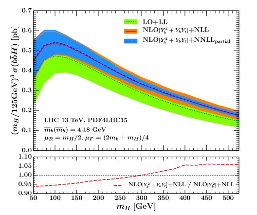
Figure 4: Matched $b\bar{b}H$ cross section as a function of $m_{H}$, comparing different orders at LO+LL (green band), NLO[$Y_{b}^{2}\!+\!Y_{b}Y_{t}$]+NLL (orange band), and NLO[$Y_{b}^{2}\!+\!Y_{b}Y_{t}$]+NNLL_partial (blue band). The cross section is rescaled by $(m_{H}/125\,\mathrm{GeV})^{3}$. The lower panel shows the ratio of the central predictions NLO[$Y_{b}^{2}\!+\!Y_{b}Y_{t}$]+NLL over NLO[$Y_{b}^{2}$]+NLL. The uncertainty bands are obtained by adding the $\{\mu_{F},\mu_{R}\}$ and $\mu_{b}$ uncertainties in quadrature.

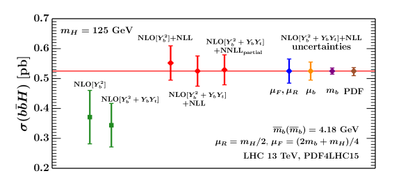
Figure 5: Comparison of the cross sections for $m_{H}=125$ GeV at the 13 TeV LHC at NLO[$Y_{b}^{2}$], NLO[$Y_{b}^{2}\!+\!Y_{b}Y_{t}$] without resummation and at NLO[$Y_{b}^{2}$]+NLL, NLO[$Y_{b}^{2}\!+\!Y_{b}Y_{t}$]+NLL, and NLO[$Y_{b}^{2}\!+\!Y_{b}Y_{t}$]+NNLL_partial. A full breakdown of the uncertainties at NLO[$Y_{b}^{2}\!+\!Y_{b}Y_{t}$]+NLL is also shown.

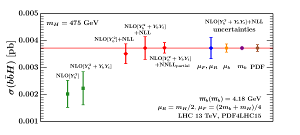
Figure 6: Comparison of the cross sections for $m_{H}=475$ GeV at the 13 TeV LHC at NLO[$Y_{b}^{2}$], NLO[$Y_{b}^{2}\!+\!Y_{b}Y_{t}$] without resummation and at NLO[$Y_{b}^{2}$]+NLL, NLO[$Y_{b}^{2}\!+\!Y_{b}Y_{t}$]+NLL, and NLO[$Y_{b}^{2}\!+\!Y_{b}Y_{t}$]+NNLL_partial. A full breakdown of the uncertainties at NLO[$Y_{b}^{2}\!+\!Y_{b}Y_{t}$]+NLL is also shown.

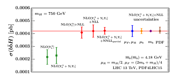
Figure 7: Comparison of the cross sections for $m_{H}=750$ GeV at the 13 TeV LHC at NLO[$Y_{b}^{2}$], NLO[$Y_{b}^{2}\!+\!Y_{b}Y_{t}$] without resummation and at NLO[$Y_{b}^{2}$]+NLL, NLO[$Y_{b}^{2}\!+\!Y_{b}Y_{t}$]+NLL, and NLO[$Y_{b}^{2}\!+\!Y_{b}Y_{t}$]+NNLL_partial. A full breakdown of the uncertainties at NLO[$Y_{b}^{2}\!+\!Y_{b}Y_{t}$]+NLL is also shown.

In this section, we present our numerical results for the inclusive $b\bar{b}H$ cross section for values of the Higgs boson mass in the range $m_{H}\in[50,750]\,\mathrm{GeV}$. We also consider values of the Higgs mass different from $m_{H}=125\,\mathrm{GeV}$, as these are relevant for BSM scenarios in which the Higgs coupling to the bottom quark is enhanced. For simplicity we always use SM couplings – the cross section in many BSM scenarios can be obtained by rescaling $Y_{b}$ by an appropriate model-dependent factor Carena:1999py ; Guasch:2003cv ; Dawson:2005vi .

We always use the simplified implementation without the strict expansion, which should still be valid at the lowest considered value of $m_{H}$. The highest value is chosen only semirandomly ATLAS-CONF-2016-018 ; CMS:2016owr . The results for the cross section at NLO[$Y_{b}^{2}$]+NLL, NLO[$Y_{b}^{2}\!+\!Y_{b}Y_{t}$]+NLL, NLO[$Y_{b}^{2}$]+NNLL_partial, and NLO[$Y_{b}^{2}\!+\!Y_{b}Y_{t}$]+NNLL_partial are given in tables 1, 2, 3, and 4, respectively. The precise definitions of the different orders are discussed in section 2. In the cross section tables we give the central value for the cross section together with the full breakdown of the perturbative uncertainties due to $\{\mu_{F},\mu_{R}\}$ and $\mu_{b}$ as well as the parametric uncertainties due to $m_{b}$ and PDFs.

For each of the fixed-order ($\mu_{F}$ and $\mu_{R}$), resummation ($\mu_{b}$), and parametric $m_{b}$ uncertainties we use the absolute value of the maximum deviation from the central result as the symmetric uncertainty. The PDF uncertainty is computed according to the PDF4LHC15 prescription as described in section 3.3 and is kept asymmetric. As discussed in section 3.1, the full perturbative uncertainty is obtained by adding the fixed-order and resummation uncertainties in quadrature. If one is only interested in the total $b\bar{b}H$ cross section, the perturbative and parametric uncertainties can be added in quadrature. In a more complicated setup, e.g., a global fit, the total perturbative, $m_{b}$, and PDF uncertainties should be treated as independent uncertainty sources (e.g. they correspond to independent nuisance parameters). This allows one to properly take into account their correlations with other predictions affected by the same physical uncertainty sources. For example, the parametric uncertainty due to $m_{b}$ or $Y_{b}$ should be correlated with the corresponding parametric uncertainty when bottom loop effects are included in $ggH$.

Our results are also illustrated in three figures. In figure 4, we show the LO+LL, NLO[$Y_{b}^{2}\!+\!Y_{b}Y_{t}$]+NLL, and NLO[$Y_{b}^{2}\!+\!Y_{b}Y_{t}$]+NNLL_partial cross sections as a function of the Higgs mass. Here, the uncertainty bands show the total perturbative uncertainty adding in quadrature the $\{\mu_{F},\mu_{R}\}$ and $\mu_{b}$ uncertainties. The important message that follows from this figure is that we can see an excellent perturbative convergence between the orders. Additionally, the band for the NLO[$Y_{b}^{2}\!+\!Y_{b}Y_{t}$]+NNLL_partial cross section is fully included within the NLO[$Y_{b}^{2}\!+\!Y_{b}Y_{t}$]+NLL band, and the central values for the two results are almost identical, which is a nice feature of our central scale choices. This pattern also gives us a good degree of confidence in the method we use to estimate the perturbative uncertainties.

These conclusions are unchanged when the $Y_{b}Y_{t}$ interference terms are omitted. In the lower panel of the figure we show the ratio of the central NLO[$Y_{b}^{2}\!+\!Y_{b}Y_{t}$]+NLL over the central NLO[$Y_{b}^{2}$]+NLL to illustrate the numerical effect of the $Y_{b}Y_{t}$ interference terms on the matched result. We see that the effect of adding the interference term is moderate but clearly noticeable in the numerical results, giving a negative contribution for $m_{H}\lesssim 300$ GeV, and a positive one for larger masses. (The small fluctuations are due to the finite integration statistics in MC@NLO when including the interference terms.)

Note that for large Higgs masses the uncertainties at NLO+NNLL_partial get significantly smaller than at NLO+NLL. As discussed in section 2.3, this is expected since for large $m_{H}$ the 5FS perturbative counting is more appropriate and in this limit the NLO+NNLL_partial formally improves the accuracy of the result, becoming as accurate as the full NNLO 5FS cross section. For smaller values around the physical Higgs mass of $m_{H}=125\,\mathrm{GeV}$, our counting is more appropriate, and only the full NNLO+NNLL should be regarded as a complete next-order result. Therefore, in this region the larger NLO+NLL uncertainty should be regarded as a safer estimate of the residual theory uncertainty. This is also nicely confirmed by the fact that in this range the NLO+NNLL_partial uncertainty is essentially as large as at NLO+NLL.

In figures 5, 6, and 7 we give a visual breakdown of the results for $m_{H}=125$ GeV, $m_{H}=475$ GeV, and $m_{H}=750\,\mathrm{GeV}$. The matched results and uncertainty contributions are equivalent to the numbers provided in the tables. In addition, we also give a comparison with the corresponding pure fixed-order results at NLO with and without $Y_{b}Y_{t}$ terms (green points). By comparing the green NLO with the red NLO+NLL points we can see that the effects of the resummation are significant, resulting in a $\sim 30\%$ increase for $m_{H}=125$ GeV, and even more at the higher Higgs masses, and moreoever this effect is not covered by the fixed-order scale variation band. This clearly shows that the resummation of $b$-quark collinear logarithms cannot be neglected for these mass values. Comparing the red points for NLO[$Y_{b}^{2}\!+\!Y_{b}Y_{t}$]+NLL and NLO[$Y_{b}^{2}\!+\!Y_{b}Y_{t}$]+NNLL_partial we see the same features as we saw in fig. 4.

The four points on the right of figures 5, 6, and 7 show the breakdown of the uncertainties for our default result at NLO[$Y_{b}^{2}\!+\!Y_{b}Y_{t}$]+NLL. Clearly, the fixed-order uncertainty estimated by the $\mu_{F}$ and $\mu_{R}$ variations is the largest source of uncertainty in the predictions, both for moderate as well as large values of $m_{H}$. The orange points show the resummation uncertainty estimated from the $\mu_{b}$ variation, which, although smaller than the fixed-order uncertainty by roughly a factor of two, is nevertheless not negligible. We also recall that at the lower LO+LL order the resummation uncertainty plays a significant role, as was shown in ref. Bonvini:2015pxa .

The parametric uncertainties due to $m_{b}$ (purple points) and PDFs (brown points) are subdominant. The $m_{b}$ uncertainties are small around $2\%$ and decrease for higher Higgs masses to around $1\%$. The (asymmetric) PDF uncertainties, computed as described in section 3.3, are around $4\%$ and smaller than both the $\{\mu_{F},\mu_{R}\}$ and $\mu_{b}$ uncertainties.

One point to emphasize is that the uncertainty which is solely due to the parametric uncertainty in $m_{b}$ is much smaller than the perturbative $\mu_{b}$ uncertainty, especially for larger Higgs masses. This shows the importance of distinguishing these two effects. If we were to identify $\mu_{b}\equiv m_{b}$, as is commonly done, we would be left to choose between two undesirable options. Either we could vary their common value in the range eq. (11), which would essentially set the $\mu_{b}$ uncertainty to zero. Or, we could vary their common value in a much larger range to account for the $\mu_{b}$ uncertainty, which however would be unjustified for $m_{b}$ and blow up the parametric $m_{b}$ uncertainty. In contrast, by identifying and separating these two uncertainty sources, we are able to properly estimate each of them.

5 Conclusions

We have presented state-of-the-art predictions for the $b\bar{b}H$ cross section at 13 TeV obtained from a matched calculation Bonvini:2015pxa that consistently combines the fixed-order (4FS) contributions (which include the full $b$-quark mass dependence) with the all-order resummation of collinear logarithms of $m_{b}/m_{H}$. We provide results with and without including the effect of the interference of top-loop induced Higgs production process with the pure bottom-induced production proportional to $Y_{b}Y_{t}$. We also study the effect of two-loop contributions that formally contribute at NNLL order, finding that they are small and their effect fully captured by the uncertainty of our default NLO+NLL result.

We perform a detailed study of several sources of uncertainty in our results, both theoretical and parametric. The perturbative uncertainty from missing higher orders is estimated by varying the hard scales $\mu_{F}$ and $\mu_{R}$, as well as the resummation scale $\mu_{b}$, which represents the threshold scale at which 4FS evolution is matched to 5FS evolution in the PDFs. We consider our resulting theory uncertainty as a reliable estimate, which is neither aggressive nor overly conservative. Furthermore, the parametric uncertainties due to the $b$-quark mass value and PDFs are evaluated. In particular, we discuss how to disentangle the unphysical dependence on the $b$-quark matching scale $\mu_{b}$ from the purely parametric dependence on the $b$-quark mass $m_{b}$, which requires the construction of dedicated 5F PDFs.

Our methodology to compute the matched prediction and to evaluate its uncertainties can be readily applied to other heavy-quark-initiated processes at the LHC. The code for our matched predictions will be available at http://www.ge.infn.it/$\sim$bonvini/bbh. Our results represent the currently most complete predictions for the $b\bar{b}H$ cross section in the Standard Model and we are looking forward to a first measurement of this process during the coming LHC Run 2.

- (1) M. Aivazis, F. I. Olness and W.-K. Tung, Leptoproduction of heavy quarks. 1. General formalism and kinematics of charged current and neutral current production processes, Phys. Rev. D 50 (1994) 3085–3101, [hep-ph/9312318].
- (2) M. Aivazis, J. C. Collins, F. I. Olness and W.-K. Tung, Leptoproduction of heavy quarks. 2. A Unified QCD formulation of charged and neutral current processes from fixed target to collider energies, Phys. Rev. D 50 (1994) 3102–3118, [hep-ph/9312319].
- (3) R. Thorne and R. Roberts, An Ordered analysis of heavy flavor production in deep inelastic scattering, Phys. Rev. D 57 (1998) 6871–6898, [hep-ph/9709442].
- (4) S. Kretzer and I. Schienbein, Heavy quark initiated contributions to deep inelastic structure functions, Phys. Rev. D 58 (1998) 094035, [hep-ph/9805233].
- (5) J. C. Collins, Hard scattering factorization with heavy quarks: A General treatment, Phys. Rev. D 58 (1998) 094002, [hep-ph/9806259].
- (6) M. Cacciari, M. Greco and P. Nason, The P(T) spectrum in heavy flavor hadroproduction, JHEP 05 (1998) 007, [hep-ph/9803400].
- (7) M. Kramer, F. I. Olness and D. E. Soper, Treatment of heavy quarks in deeply inelastic scattering, Phys. Rev. D 62 (2000) 096007, [hep-ph/0003035].
- (8) W.-K. Tung, S. Kretzer and C. Schmidt, Open heavy flavor production in QCD: Conceptual framework and implementation issues, J. Phys. G 28 (2002) 983–996, [hep-ph/0110247].
- (9) R. Thorne, A Variable-flavor number scheme for NNLO, Phys. Rev. D 73 (2006) 054019, [hep-ph/0601245].
- (10) S. Forte, E. Laenen, P. Nason and J. Rojo, Heavy quarks in deep-inelastic scattering, Nucl.Phys. B834 (2010) 116–162, [arXiv:1001.2312].
- (11) M. Guzzi, P. M. Nadolsky, H.-L. Lai and C.-P. Yuan, General-Mass Treatment for Deep Inelastic Scattering at Two-Loop Accuracy, Phys. Rev. D 86 (2012) 053005, [arXiv:1108.5112].
- (12) A. H. Hoang, P. Pietrulewicz and D. Samitz, Variable Flavor Number Scheme for Final State Jets in DIS, Phys. Rev. D 93 (2016) 034034, [arXiv:1508.04323].
- (13) R. D. Ball, M. Bonvini and L. Rottoli, Charm in Deep-Inelastic Scattering, JHEP 11 (2015) 122, [arXiv:1510.02491].
- (14) T. Han, J. Sayre and S. Westhoff, Top-Quark Initiated Processes at High-Energy Hadron Colliders, JHEP 04 (2015) 145, [arXiv:1411.2588].
- (15) S. Forte, D. Napoletano and M. Ubiali, Higgs production in bottom-quark fusion in a matched scheme, arXiv:1508.01529.
- (16) M. Bonvini, A. S. Papanastasiou and F. J. Tackmann, Resummation and matching of b-quark mass effects in production, JHEP 11 (2015) 196, [arXiv:1508.03288].
- (17) D. Dicus, T. Stelzer, Z. Sullivan and S. Willenbrock, Higgs boson production in association with bottom quarks at next-to-leading order, Phys. Rev. D 59 (1999) 094016, [hep-ph/9811492].
- (18) C. Balazs, H.-J. He and C. Yuan, QCD corrections to scalar production via heavy quark fusion at hadron colliders, Phys. Rev. D 60 (1999) 114001, [hep-ph/9812263].
- (19) R. V. Harlander and W. B. Kilgore, Higgs boson production in bottom quark fusion at next-to-next-to leading order, Phys. Rev. D 68 (2003) 013001, [hep-ph/0304035].
- (20) S. Bühler, F. Herzog, A. Lazopoulos and R. Müller, The fully differential hadronic production of a Higgs boson via bottom quark fusion at NNLO, JHEP 07 (2012) 115, [arXiv:1204.4415].
- (21) R. V. Harlander, S. Liebler and H. Mantler, SusHi: A program for the calculation of Higgs production in gluon fusion and bottom-quark annihilation in the Standard Model and the MSSM, Comput. Phys. Commun. 184 (2013) 1605–1617, [arXiv:1212.3249].
- (22) S. Dittmaier, M. Kramer and M. Spira, Higgs radiation off bottom quarks at the Tevatron and the CERN LHC, Phys. Rev. D 70 (2004) 074010, [hep-ph/0309204].
- (23) S. Dawson, C. B. Jackson, L. Reina and D. Wackeroth, Exclusive Higgs boson production with bottom quarks at hadron colliders, Phys. Rev. D 69 (2004) 074027, [hep-ph/0311067].
- (24) M. Wiesemann, R. Frederix, S. Frixione, V. Hirschi, F. Maltoni and P. Torrielli, Higgs production in association with bottom quarks, JHEP 02 (2015) 132, [arXiv:1409.5301].
- (25) R. Harlander, M. Kramer and M. Schumacher, Bottom-quark associated Higgs-boson production: reconciling the four- and five-flavour scheme approach, arXiv:1112.3478.
- (26) J. Alwall, R. Frederix, S. Frixione, V. Hirschi, F. Maltoni, O. Mattelaer et al., The automated computation of tree-level and next-to-leading order differential cross sections, and their matching to parton shower simulations, JHEP 07 (2014) 079, [arXiv:1405.0301].
- (27) F. Maltoni, Z. Sullivan and S. Willenbrock, Higgs-boson production via bottom-quark fusion, Phys. Rev. D 67 (2003) 093005, [hep-ph/0301033].
- (28) F. Maltoni, T. McElmurry and S. Willenbrock, Inclusive production of a Higgs or boson in association with heavy quarks, Phys. Rev. D 72 (2005) 074024, [hep-ph/0505014].
- (29) F. Maltoni, G. Ridolfi and M. Ubiali, b-initiated processes at the LHC: a reappraisal, JHEP 07 (2012) 022, [arXiv:1203.6393]. [Erratum: JHEP04,095(2013)].
- (30) R. V. Harlander, Higgs production in heavy quark annihilation through next-to-next-to-leading order QCD, arXiv:1512.04901.
- (31) Particle Data Group collaboration, K. A. Olive et al., Review of Particle Physics, Chin. Phys. C38 (2014) 090001.
- (32) A. Denner, S. Dittmaier, M. Grazzini, R. V. Harlander, R. S. Thorne, M. Spira et al., Standard Model input parameters for Higgs physics, . LHCHXSWG-INT-2015-006.
- (33) V. Bertone, S. Carrazza and J. Rojo, APFEL: A PDF Evolution Library with QED corrections, Comput. Phys. Commun. 185 (2014) 1647–1668, [arXiv:1310.1394].
- (34) L. A. Harland-Lang, A. D. Martin, P. Motylinski and R. S. Thorne, Charm and beauty quark masses in the MMHT2014 global PDF analysis, Eur. Phys. J. C76 (2016) 10, [arXiv:1510.02332].
- (35) J. Butterworth et al., PDF4LHC recommendations for LHC Run II, J. Phys. G43 (2016) 023001, [arXiv:1510.03865].
- (36) S. Carrazza, J. I. Latorre, J. Rojo and G. Watt, A compression algorithm for the combination of PDF sets, Eur. Phys. J. C75 (2015) 474, [arXiv:1504.06469].
- (37) NNPDF collaboration, R. D. Ball et al., Parton distributions for the LHC Run II, JHEP 04 (2015) 040, [arXiv:1410.8849].
- (38) L. A. Harland-Lang, A. D. Martin, P. Motylinski and R. S. Thorne, Parton distributions in the LHC era: MMHT 2014 PDFs, Eur. Phys. J. C75 (2015) 204, [arXiv:1412.3989].
- (39) S. Dulat, T.-J. Hou, J. Gao, M. Guzzi, J. Huston, P. Nadolsky et al., New parton distribution functions from a global analysis of quantum chromodynamics, Phys. Rev. D 93 (2016) 033006, [arXiv:1506.07443].
- (40) M. Carena, D. Garcia, U. Nierste and C. E. M. Wagner, Effective Lagrangian for the interaction in the MSSM and charged Higgs phenomenology, Nucl. Phys. B577 (2000) 88–120, [hep-ph/9912516].
- (41) J. Guasch, P. Hafliger and M. Spira, MSSM Higgs decays to bottom quark pairs revisited, Phys. Rev. D68 (2003) 115001, [hep-ph/0305101].
- (42) S. Dawson, C. B. Jackson, L. Reina and D. Wackeroth, Higgs production in association with bottom quarks at hadron colliders, Mod. Phys. Lett. A21 (2006) 89–110, [hep-ph/0508293].
- (43) ATLAS Collaboration, Search for resonances in diphoton events with the ATLAS detector at = 13 TeV, . ATLAS-CONF-2016-018.
- (44) CMS Collaboration, Search for new physics in high mass diphoton events in of proton-proton collisions at and combined interpretation of searches at and , . CMS-PAS-EXO-16-018.