A Tight Bound of Hard Thresholding

Jie Shen
Rutgers University
Piscataway, NJ 08854, USA
js2007@rutgers.edu
   Ping Li
Baidu Research
Bellevue, WA 98004, USA
pingli98@gmail.com
Abstract

This paper is concerned with the hard thresholding operator which sets all but the k𝑘k largest absolute elements of a vector to zero. We establish a tight bound to quantitatively characterize the deviation of the thresholded solution from a given signal. Our theoretical result is universal in the sense that it holds for all choices of parameters, and the underlying analysis depends only on fundamental arguments in mathematical optimization. We discuss the implications for two domains:

Compressed Sensing.  On account of the crucial estimate, we bridge the connection between the restricted isometry property (RIP) and the sparsity parameter for a vast volume of hard thresholding based algorithms, which renders an improvement on the RIP condition especially when the true sparsity is unknown. This suggests that in essence, many more kinds of sensing matrices or fewer measurements are admissible for the data acquisition procedure.

Machine Learning.  In terms of large-scale machine learning, a significant yet challenging problem is learning accurate sparse models in an efficient manner. In stark contrast to prior work that attempted the 1subscript1\ell_{1}-relaxation for promoting sparsity, we present a novel stochastic algorithm which performs hard thresholding in each iteration, hence ensuring such parsimonious solutions. Equipped with the developed bound, we prove the global linear convergence for a number of prevalent statistical models under mild assumptions, even though the problem turns out to be non-convex.

Keywords: sparsity, hard thresholding, compressed sensing, stochastic optimization

1 Introduction

Over the last two decades, pursuing sparse representations has emerged as a fundamental technique throughout bioinformatics [OF97], statistics [Tib96, EHJT04], signal processing [CDS98, DET06, Don06, CW08] and mathematical science [CRPW12], to name just a few. In order to obtain a sparse solution, a plethora of practical algorithms have been presented, among which two prominent examples are greedy pursuit and convex relaxation [TW10]. For instance, as one of the earliest greedy algorithms, orthogonal matching pursuit (OMP) [PRK93] repeatedly picks a coordinate as the potential support of a solution. While OMP may fail for some deterministic sensing matrices, [Tro04, TG07] showed that it recovers the true signal with high probability when using random matrices such as Gaussian. Inspired by the success of OMP, the two concurrent work of compressive sampling matching pursuit (CoSaMP) [NT09] and subspace pursuit (SP) [DM09] made improvement by selecting multiple coordinates followed by a pruning step in each iteration, and the recovery condition was framed under the restricted isometry property (RIP) [CT05]. Interestingly, the more careful selection strategy of CoSaMP and SP leads to an optimal sample complexity. The iterative hard thresholding (IHT) algorithm [DDM04, BD08, BD09] gradually refines the iterates by gradient descent along with truncation. [Fou11] then developed a concise algorithm termed hard thresholding pursuit (HTP), which combined the idea of CoSaMP and IHT, and showed that HTP is superior to both in terms of the RIP condition. [JTD11] proposed an interesting variant of the HTP algorithm and obtained a sharper RIP result. Recently, [BRB13] and [YLZ18] respectively extended CoSaMP and HTP to general objective functions, for which a global convergence was established.

Since the sparsity constraint counts the number of non-zero components which renders the problem non-convex, the 1subscript1\ell_{1}-norm was suggested as a convex relaxation dating back to basis pursuit [CDS98, DT08] and Lasso [Tib96]. The difference is that Lasso looks for an 1subscript1\ell_{1}-norm constrained solution that minimizes the residual while the principle of basis pursuit is to find a signal with minimal 1subscript1\ell_{1}-norm that fits the observation data. [CT05] carried out a detailed analysis on the recovery performance of basis pursuit. Another popular estimator in the high-dimensional statistics is the Dantzig selector [CT07] which, instead of constraining the residual of the linear model, penalizes the maximum magnitude of the gradient. From a computational perspective, both basis pursuit and Dantzig selector can be solved by linear programming, while Lasso is formulated as a quadratic problem. Interestingly, under the RIP condition or the uniform uncertainty assumption [CRT06], a series of work showed that exact recovery by convex programs is possible as soon as the observation noise vanishes [CT05, Can08, Wai09, CWX10, Fou12].

In this paper, we are interested in the hard thresholding (HT) operator underlying a large body of the developed algorithms in compressed sensing (e.g., IHT, CoSaMP, SP), machine learning [YZ13], and statistics [Ma13]. Our motivation is two-fold. From a high level, compared to the convex programs, these HT-based algorithms are always orders of magnitude computationally more efficient, hence more practical for large-scale problems [TW10]. Nevertheless, they usually require a more stringent condition to guarantee the success. This naturally raises an interesting question of whether we can derive milder conditions for HT-based algorithms to achieve the best of the two worlds. For practitioners, to address the huge volume of data, a popular strategy in machine learning is to appeal to stochastic algorithms that sequentially update the solution. However, as many researchers observed [LLZ09, DS09, Xia10], it is hard for the 1subscript1\ell_{1}-based stochastic algorithms to preserve the sparse structure of the solution as the batch solvers do. This immediately poses the question of whether we are able to apply the principal idea of hard thresholding to stochastic algorithms while still ensuring a fast convergence.

To elaborate the problem more precisely, let us first turn to some basic properties of hard thresholding along with simple yet illustrative cases. For a general vector 𝒃d𝒃superscript𝑑\boldsymbol{b}\in\mathbb{R}^{d}, the hard thresholded signal k(𝒃)subscript𝑘𝒃\mathcal{H}_{k}\left(\boldsymbol{b}\right) is formed by setting all but the largest (in magnitude) k𝑘k elements of 𝒃𝒃\boldsymbol{b} to zero. Ties are broken lexicographically. Hence, the hard thresholded signal k(𝒃)subscript𝑘𝒃\mathcal{H}_{k}\left(\boldsymbol{b}\right) is always k𝑘k-sparse, i.e., the number of non-zero components does not exceed k𝑘k. Moreover, the resultant signal k(𝒃)subscript𝑘𝒃\mathcal{H}_{k}\left(\boldsymbol{b}\right) is a best k𝑘k-sparse approximation to 𝒃𝒃\boldsymbol{b} in terms of any psubscript𝑝\ell_{p} norm (p1𝑝1p\geq 1). That is, for any k𝑘k-sparse vector 𝒙𝒙\boldsymbol{x}

k(𝒃)𝒃p𝒙𝒃p.subscriptdelimited-∥∥subscript𝑘𝒃𝒃𝑝subscriptdelimited-∥∥𝒙𝒃𝑝\lVert{\mathcal{H}_{k}\left(\boldsymbol{b}\right)-\boldsymbol{b}}\rVert_{p}\leq\lVert{\boldsymbol{x}-\boldsymbol{b}}\rVert_{p}.

In view of the above inequality, a broadly used bound in the literature for the deviation of the thresholded signal is as follows:

k(𝒃)𝒙22𝒃𝒙2.subscriptdelimited-∥∥subscript𝑘𝒃𝒙22subscriptdelimited-∥∥𝒃𝒙2\left\lVert\mathcal{H}_{k}\left(\boldsymbol{b}\right)-\boldsymbol{x}\right\rVert_{2}\leq 2\left\lVert\boldsymbol{b}-\boldsymbol{x}\right\rVert_{2}. (1.1)

To gain intuition on the utility of (1.1) and to spell out the importance of offering a tight bound for it, let us consider the compressed sensing problem as an example for which we aim to recover the true sparse signal 𝒙𝒙\boldsymbol{x} from its linear measurements. Here, 𝒃𝒃\boldsymbol{b} is a good but dense approximation to 𝒙𝒙\boldsymbol{x} obtained by, e.g., full gradient descent. Then (1.1) justifies that in order to obtain a structured (i.e., sparse) approximation by hard thresholding, the distance of the iterate to the true signal 𝒙𝒙\boldsymbol{x} is upper bounded by a multiple of 222 to the one before. For comparison, it is worth mentioning that 1subscript1\ell_{1}-based convex algorithms usually utilize the soft thresholding operator which enjoys the non-expansiveness property [DBL14], i.e., the iterate becomes closer to the optimum after projection. This salient feature might partially attribute to the wide range of applications of the 1subscript1\ell_{1}-regularized formulations. Hence, to derive comparable performance guarantee, tightening the bound (1.1) is crucial in that it controls how much deviation the hard thresholding operator induces. This turns out to be more demanding for stochastic gradient methods, where the proxy 𝒃𝒃\boldsymbol{b} itself is affected by the randomness of sample realization. In other words, since 𝒃𝒃\boldsymbol{b} does not minimize the objective function (it only optimizes the objective in expectation), the deviation (1.1) makes it more challenging to analyze the convergence behavior. As an example, [NNW14] proposed a stochastic solver for general sparsity-constrained programs but suffered a non-vanishing optimization error due to randomness. This indicates that to mitigate the randomness barrier, we have to seek a better bound to control the precision of the thresholded solution and the variance.

1.1 Summary of Contributions

In this work, we make three contributions:

  1. 1.

    We examine the tightness of (1.1) that has been used for a decade in the literature and show that the equality therein will never be attained. We then improve this bound and quantitatively characterize that the deviation is inversely proportional to the value of k𝑘\sqrt{k}. Our bound is tight, in the sense that the equality we build can be attained for specific signals, hence cannot be improved if no additional information is available. Our bound is universal in the sense that it holds for all choices of k𝑘k-sparse signals 𝒙𝒙\boldsymbol{x} and for general signals 𝒃𝒃\boldsymbol{b}.

  2. 2.

    Owing to the tight estimate, we demonstrate how the RIP (or RIP-like) condition assumed by a wide range of hard thresholding based algorithms can be relaxed. In the context of compressed sensing, it means that in essence, many more kinds of sensing matrices or fewer measurements can be utilized for data acquisition. For machine learning, it suggests that existing algorithms are capable of handling more difficult statistical models.

  3. 3.

    Finally, we present an computationally efficient algorithm that applies hard thresholding in large-scale setting and we prove its linear convergence to a global optimum up to the statistical precision of the problem. We also prove that with sufficient samples, our algorithm identifies the true parameter for prevalent statistical models. Returning to (1.1), our analysis shows that only when the deviation is controlled below the multiple of 1.151.151.15 can such an algorithm succeed. This immediately implies that the conventional bound (1.1) is not applicable in the challenging scenario.

1.2 Notation

Before delivering the algorithm and main theoretical results, let us instate several pieces of notation that are involved throughout the paper. We use bold lowercase letters, e.g., 𝒗𝒗\boldsymbol{v}, to denote a vector (either column or row) and its i𝑖ith element is denoted by visubscript𝑣𝑖v_{i}. The 2subscript2\ell_{2}-norm of a vector 𝒗𝒗\boldsymbol{v} is denoted by 𝒗2subscriptdelimited-∥∥𝒗2\left\lVert\boldsymbol{v}\right\rVert_{2}. The support set of 𝒗𝒗\boldsymbol{v}, i.e., indices of non-zeros, is denoted by supp(𝒗)supp𝒗\mathrm{supp}\left(\boldsymbol{v}\right) whose cardinality is written as |supp(𝒗)|supp𝒗\left\lvert\mathrm{supp}\left(\boldsymbol{v}\right)\right\rvert or 𝒗0subscriptdelimited-∥∥𝒗0\left\lVert\boldsymbol{v}\right\rVert_{0}. We write bold capital letters such as 𝑴𝑴\boldsymbol{M} for matrices and its (i,j)𝑖𝑗(i,j)-th entry is denoted by mijsubscript𝑚𝑖𝑗m_{ij}. The capital upright letter CC\mathrm{{C}} and its subscript variants (e.g., C0,C1subscriptC0subscriptC1\mathrm{{C}}_{0},\mathrm{{C}}_{1}) are reserved for absolute constants whose values may change from appearance to appearance.

For an integer d>0𝑑0d>0, suppose that ΩΩ\Omega is a subset of {1, 2,,d}12𝑑\{1,\ 2,\ \dots,\ d\}. Then for a general vector 𝒗d𝒗superscript𝑑\boldsymbol{v}\in\mathbb{R}^{d}, we define 𝒫Ω()subscript𝒫Ω\mathcal{P}_{\Omega}\left(\cdot\right) as the orthogonal projection onto the support set ΩΩ\Omega which retains elements contained in ΩΩ\Omega and sets others to zero. That is,

(𝒫Ω(𝒗))i={vi,ifiΩ,0,otherwise.subscriptsubscript𝒫Ω𝒗𝑖casessubscript𝑣𝑖if𝑖Ω0otherwise\displaystyle\left(\mathcal{P}_{\Omega}\left(\boldsymbol{v}\right)\right)_{i}=\begin{cases}v_{i},\ &\text{if}\ i\in\Omega,\\ 0,\ &\text{otherwise}.\end{cases}

In particular, let ΓΓ\Gamma be the support set indexing the k𝑘k largest absolute components of 𝒗𝒗\boldsymbol{v}. In this way, the hard thresholding operator is given by

k(𝒗)=𝒫Γ(𝒗).subscript𝑘𝒗subscript𝒫Γ𝒗\mathcal{H}_{k}\left(\boldsymbol{v}\right)=\mathcal{P}_{\Gamma}(\boldsymbol{v}).

We will also use the orthogonal projection of a vector 𝒗𝒗\boldsymbol{v} onto an 2subscript2\ell_{2}-ball with radius ω𝜔\omega. That is,

Πω(𝒗)=𝒗max{1,𝒗2/ω}.subscriptΠ𝜔𝒗𝒗1subscriptdelimited-∥∥𝒗2𝜔\Pi_{\omega}(\boldsymbol{v})=\frac{\boldsymbol{v}}{\max\{1,\left\lVert\boldsymbol{v}\right\rVert_{2}/\omega\}}.

1.3 Roadmap

We present the key tight bound for hard thresholding in Section 2, along with a justification why the conventional bound (1.1) is not tight. We then discuss the implications of the developed tight bound to compressed sensing and machine learning in Section 3, which shows that the RIP or RIP-like condition can be improved for a number of popular algorithms. Thanks to our new estimation, Section 4 develops a novel stochastic algorithm which applies hard thresholding to large-scale problems and establishes the global linear convergence. A comprehensive empirical study on the tasks of sparse recovery and binary classification is carried out in Section 5. Finally, We conclude the paper in Section 6 and all the proofs are deferred to the appendix.

2 The Key Bound

We argue that the conventional bound (1.1) is not tight, in the sense that the equality therein can hardly be attained. To see this, recall how the bound was derived for a k𝑘k-sparse signal 𝒙𝒙\boldsymbol{x} and a general one 𝒃𝒃\boldsymbol{b}:

k(𝒃)𝒙2=k(𝒃)𝒃+𝒃𝒙2ξk(𝒃)𝒃2+𝒃𝒙22𝒃𝒙2,subscriptdelimited-∥∥subscript𝑘𝒃𝒙2subscriptdelimited-∥∥subscript𝑘𝒃𝒃𝒃𝒙2superscript𝜉subscriptdelimited-∥∥subscript𝑘𝒃𝒃2subscriptdelimited-∥∥𝒃𝒙22subscriptdelimited-∥∥𝒃𝒙2\left\lVert\mathcal{H}_{k}\left(\boldsymbol{b}\right)-\boldsymbol{x}\right\rVert_{2}=\left\lVert\mathcal{H}_{k}\left(\boldsymbol{b}\right)-\boldsymbol{b}+\boldsymbol{b}-\boldsymbol{x}\right\rVert_{2}\stackrel{{\scriptstyle\xi}}{{\leq}}\left\lVert\mathcal{H}_{k}\left(\boldsymbol{b}\right)-\boldsymbol{b}\right\rVert_{2}+\left\lVert\boldsymbol{b}-\boldsymbol{x}\right\rVert_{2}\leq 2\left\lVert\boldsymbol{b}-\boldsymbol{x}\right\rVert_{2},

where the last inequality holds because k(𝒃)subscript𝑘𝒃\mathcal{H}_{k}\left(\boldsymbol{b}\right) is a best k𝑘k-sparse approximation to 𝒃𝒃\boldsymbol{b}. The major issue occurs in ξ𝜉\xi. Though it is the well-known triangle inequality and the equality could be attained if there is no restriction on the signals 𝒙𝒙\boldsymbol{x} and 𝒃𝒃\boldsymbol{b}, we remind here that the signal 𝒙𝒙\boldsymbol{x} does have a specific structure – it is k𝑘k-sparse. Note that in order to fulfill the equality in ξ𝜉\xi, we must have k(𝒃)𝒃=γ(𝒃𝒙)subscript𝑘𝒃𝒃𝛾𝒃𝒙\mathcal{H}_{k}\left(\boldsymbol{b}\right)-\boldsymbol{b}=\gamma(\boldsymbol{b}-\boldsymbol{x}) for some γ0𝛾0\gamma\geq 0, that is,

k(𝒃)=(γ+1)𝒃γ𝒙.subscript𝑘𝒃𝛾1𝒃𝛾𝒙\mathcal{H}_{k}\left(\boldsymbol{b}\right)=(\gamma+1)\boldsymbol{b}-\gamma\boldsymbol{x}. (2.1)

One may verify that the above equality holds if and only if

𝒙=𝒃=k(𝒃).𝒙𝒃subscript𝑘𝒃\boldsymbol{x}=\boldsymbol{b}=\mathcal{H}_{k}\left(\boldsymbol{b}\right). (2.2)

To see this, let ΩΩ\Omega be the support set of k(𝒃)subscript𝑘𝒃\mathcal{H}_{k}\left(\boldsymbol{b}\right) and Ω¯¯Ω\overline{\Omega} be the complement. Let 𝒃1=𝒫Ω(𝒃)=k(𝒃)subscript𝒃1subscript𝒫Ω𝒃subscript𝑘𝒃\boldsymbol{b}_{1}=\mathcal{P}_{\Omega}\left(\boldsymbol{b}\right)=\mathcal{H}_{k}\left(\boldsymbol{b}\right) and 𝒃2=𝒫Ω¯(𝒃)subscript𝒃2subscript𝒫¯Ω𝒃\boldsymbol{b}_{2}=\mathcal{P}_{\overline{\Omega}}(\boldsymbol{b}). Likewise, we define 𝒙1subscript𝒙1\boldsymbol{x}_{1} and 𝒙2subscript𝒙2\boldsymbol{x}_{2} as the components of 𝒙𝒙\boldsymbol{x} supported on ΩΩ\Omega and Ω¯¯Ω\overline{\Omega} respectively. Hence, (2.1) indicates 𝒙1=𝒃1subscript𝒙1subscript𝒃1\boldsymbol{x}_{1}=\boldsymbol{b}_{1} and 𝒙2=(1+γ1)𝒃2subscript𝒙21superscript𝛾1subscript𝒃2\boldsymbol{x}_{2}=(1+\gamma^{-1})\boldsymbol{b}_{2} where we assume γ>0𝛾0\gamma>0 since γ=0𝛾0\gamma=0 immediately implies k(𝒃)=𝒃subscript𝑘𝒃𝒃\mathcal{H}_{k}\left(\boldsymbol{b}\right)=\boldsymbol{b} and hence the equality of (1.1) does not hold. If 𝒃10<ksubscriptdelimited-∥∥subscript𝒃10𝑘\left\lVert\boldsymbol{b}_{1}\right\rVert_{0}<k, then we have 𝒙2=𝒃2=𝟎subscript𝒙2subscript𝒃20\boldsymbol{x}_{2}=\boldsymbol{b}_{2}=\boldsymbol{0} since 𝒃1subscript𝒃1\boldsymbol{b}_{1} contains the k𝑘k largest absolute elements of 𝒃𝒃\boldsymbol{b}. Otherwise, the fact that 𝒙0ksubscriptdelimited-∥∥𝒙0𝑘\left\lVert\boldsymbol{x}\right\rVert_{0}\leq k and 𝒙1=𝒃1subscript𝒙1subscript𝒃1\boldsymbol{x}_{1}=\boldsymbol{b}_{1} implies 𝒙2=𝟎subscript𝒙20\boldsymbol{x}_{2}=\boldsymbol{0}, and hence 𝒃2subscript𝒃2\boldsymbol{b}_{2}. Therefore, we obtain (2.2).

When (2.2) happens, however, we in reality have k(𝒃)𝒙2=𝒃𝒙2=0subscriptdelimited-∥∥subscript𝑘𝒃𝒙2subscriptdelimited-∥∥𝒃𝒙20\left\lVert\mathcal{H}_{k}\left(\boldsymbol{b}\right)-\boldsymbol{x}\right\rVert_{2}=\left\lVert\boldsymbol{b}-\boldsymbol{x}\right\rVert_{2}=0. In other words, the factor of 222 in (1.1) can essentially be replaced with an arbitrary constant! In this sense, we conclude that the bound (1.1) is not tight. Our new estimate for hard thresholding is as follows:

Theorem 1 (Tight Bound for Hard Thresholding).

Let 𝐛d𝐛superscript𝑑\boldsymbol{b}\in\mathbb{R}^{d} be an arbitrary vector and 𝐱d𝐱superscript𝑑\boldsymbol{x}\in\mathbb{R}^{d} be any K𝐾K-sparse signal. For any kK𝑘𝐾k\geq K, we have the following bound:

k(𝒃)𝒙2ν𝒃𝒙2,ν=1+ρ+(4+ρ)ρ2,ρ=min{K,dk}kK+min{K,dk}.formulae-sequencesubscriptdelimited-∥∥subscript𝑘𝒃𝒙2𝜈subscriptdelimited-∥∥𝒃𝒙2formulae-sequence𝜈1𝜌4𝜌𝜌2𝜌𝐾𝑑𝑘𝑘𝐾𝐾𝑑𝑘\left\lVert\mathcal{H}_{k}\left(\boldsymbol{b}\right)-\boldsymbol{x}\right\rVert_{2}\leq\sqrt{\nu}\left\lVert\boldsymbol{b}-\boldsymbol{x}\right\rVert_{2},\quad\nu=1+\frac{\rho+\sqrt{\left(4+\rho\right)\rho}}{2},\quad\rho=\frac{\min\{K,d-k\}}{k-K+\min\{K,d-k\}}.

In particular, our bound is tight in the sense that there exist specific vectors of 𝐛𝐛\boldsymbol{b} and 𝐱𝐱\boldsymbol{x} such that the equality holds.

Remark 2 (Maximum of ν𝜈\nu).

In contrast to the constant bound (1.1), our result asserts that the deviation resulting from hard thresholding is inversely proportional to k𝑘\sqrt{k} (when Kdk𝐾𝑑𝑘K\leq d-k) in a universal manner. When k𝑘k tends to d𝑑d, ρ𝜌\rho is given by (dk)/(dK)𝑑𝑘𝑑𝐾(d-k)/(d-K) which is still decreasing with respect to k𝑘k. Thus, the maximum value of ρ𝜌\rho equals one. Even in this case, we find that νmax=1+5+12=5+121.618subscript𝜈15125121.618\sqrt{\nu_{\max}}=\sqrt{1+\frac{\sqrt{5}+1}{2}}=\frac{\sqrt{5}+1}{2}\approx 1.618.

Remark 3.

Though for some batch algorithms such as IHT and CoSaMP, the constant bound (1.1) suffices to establish the convergence due to specific conditions, we show in Section 4 that it cannot ensure the global convergence for stochastic algorithms.

Remark 4.

When 𝒙𝒙\boldsymbol{x} is not exactly K𝐾K-sparse, we still can bound the error by k(𝒃)𝒙2k(𝒃)k(𝒙)2+k(𝒙)𝒙2subscriptdelimited-∥∥subscript𝑘𝒃𝒙2subscriptdelimited-∥∥subscript𝑘𝒃subscript𝑘𝒙2subscriptdelimited-∥∥subscript𝑘𝒙𝒙2\left\lVert\mathcal{H}_{k}\left(\boldsymbol{b}\right)-\boldsymbol{x}\right\rVert_{2}\leq\left\lVert\mathcal{H}_{k}\left(\boldsymbol{b}\right)-\mathcal{H}_{k}\left(\boldsymbol{x}\right)\right\rVert_{2}+\left\lVert\mathcal{H}_{k}\left(\boldsymbol{x}\right)-\boldsymbol{x}\right\rVert_{2}. Thus, without loss of generality, we assumed that the signal 𝒙𝒙\boldsymbol{x} is K𝐾K-sparse.

Proof.

(Sketch) Our bound follows from fully exploring the sparsity pattern of the signals and from fundamental arguments in optimization. Denote

𝒘:=k(𝒃).assign𝒘subscript𝑘𝒃\boldsymbol{w}:=\mathcal{H}_{k}\left(\boldsymbol{b}\right).

Let ΩΩ\Omega be the support set of 𝒘𝒘\boldsymbol{w} and let Ω¯¯Ω\overline{\Omega} be its complement. We immediately have 𝒫Ω(𝒃)=𝒘subscript𝒫Ω𝒃𝒘\mathcal{P}_{\Omega}\left(\boldsymbol{b}\right)=\boldsymbol{w}. Let ΩsuperscriptΩ\Omega^{\prime} be the support set of 𝒙𝒙\boldsymbol{x}. Define

𝒃1=𝒫Ω\Ω(𝒃),𝒃2=𝒫ΩΩ(𝒃),𝒃3=𝒫Ω¯\Ω(𝒃),𝒃4=𝒫Ω¯Ω(𝒃).formulae-sequencesubscript𝒃1subscript𝒫\ΩsuperscriptΩ𝒃formulae-sequencesubscript𝒃2subscript𝒫ΩsuperscriptΩ𝒃formulae-sequencesubscript𝒃3subscript𝒫\¯ΩsuperscriptΩ𝒃subscript𝒃4subscript𝒫¯ΩsuperscriptΩ𝒃\boldsymbol{b}_{1}=\mathcal{P}_{\Omega\backslash\Omega^{\prime}}\left(\boldsymbol{b}\right),\quad\boldsymbol{b}_{2}=\mathcal{P}_{\Omega\cap\Omega^{\prime}}\left(\boldsymbol{b}\right),\quad\boldsymbol{b}_{3}=\mathcal{P}_{\overline{\Omega}\backslash\Omega^{\prime}}\left(\boldsymbol{b}\right),\quad\boldsymbol{b}_{4}=\mathcal{P}_{\overline{\Omega}\cap\Omega^{\prime}}\left(\boldsymbol{b}\right).

Likewise, we define 𝒙isubscript𝒙𝑖\boldsymbol{x}_{i} and 𝒘isubscript𝒘𝑖\boldsymbol{w}_{i} for 1i41𝑖41\leq i\leq 4. Due to the construction, we have 𝒘1=𝒃1,𝒘2=𝒃2,𝒘3=𝒘4=𝒙1=𝒙3=𝟎formulae-sequencesubscript𝒘1subscript𝒃1formulae-sequencesubscript𝒘2subscript𝒃2subscript𝒘3subscript𝒘4subscript𝒙1subscript𝒙30\boldsymbol{w}_{1}=\boldsymbol{b}_{1},\boldsymbol{w}_{2}=\boldsymbol{b}_{2},\boldsymbol{w}_{3}=\boldsymbol{w}_{4}=\boldsymbol{x}_{1}=\boldsymbol{x}_{3}=\boldsymbol{0}. Our goal is to estimate the maximum value of 𝒘𝒙22/𝒃𝒙22superscriptsubscriptdelimited-∥∥𝒘𝒙22superscriptsubscriptdelimited-∥∥𝒃𝒙22\left\lVert\boldsymbol{w}-\boldsymbol{x}\right\rVert_{2}^{2}/\left\lVert\boldsymbol{b}-\boldsymbol{x}\right\rVert_{2}^{2}. It is easy to show that when attaining the maximum, 𝒃32subscriptdelimited-∥∥subscript𝒃32\left\lVert\boldsymbol{b}_{3}\right\rVert_{2} must be zero. Denote

γ:=𝒘𝒙22𝒃𝒙22=𝒃122+𝒃2𝒙222+𝒙422𝒃122+𝒃2𝒙222+𝒃4𝒙422.assign𝛾superscriptsubscriptdelimited-∥∥𝒘𝒙22superscriptsubscriptdelimited-∥∥𝒃𝒙22superscriptsubscriptdelimited-∥∥subscript𝒃122superscriptsubscriptdelimited-∥∥subscript𝒃2subscript𝒙222superscriptsubscriptdelimited-∥∥subscript𝒙422superscriptsubscriptdelimited-∥∥subscript𝒃122superscriptsubscriptdelimited-∥∥subscript𝒃2subscript𝒙222superscriptsubscriptdelimited-∥∥subscript𝒃4subscript𝒙422\gamma:=\frac{\left\lVert\boldsymbol{w}-\boldsymbol{x}\right\rVert_{2}^{2}}{\left\lVert\boldsymbol{b}-\boldsymbol{x}\right\rVert_{2}^{2}}=\frac{\left\lVert\boldsymbol{b}_{1}\right\rVert_{2}^{2}+\left\lVert\boldsymbol{b}_{2}-\boldsymbol{x}_{2}\right\rVert_{2}^{2}+\left\lVert\boldsymbol{x}_{4}\right\rVert_{2}^{2}}{\left\lVert\boldsymbol{b}_{1}\right\rVert_{2}^{2}+\left\lVert\boldsymbol{b}_{2}-\boldsymbol{x}_{2}\right\rVert_{2}^{2}+\left\lVert\boldsymbol{b}_{4}-\boldsymbol{x}_{4}\right\rVert_{2}^{2}}. (2.3)

Note that the variables here only involve 𝒙𝒙\boldsymbol{x} and 𝒃𝒃\boldsymbol{b}. Arranging the equation we obtain

(γ1)𝒃2𝒙222+γ𝒃4𝒙422𝒙422+(γ1)𝒃122=0.𝛾1superscriptsubscriptdelimited-∥∥subscript𝒃2subscript𝒙222𝛾superscriptsubscriptdelimited-∥∥subscript𝒃4subscript𝒙422superscriptsubscriptdelimited-∥∥subscript𝒙422𝛾1superscriptsubscriptdelimited-∥∥subscript𝒃1220(\gamma-1)\left\lVert\boldsymbol{b}_{2}-\boldsymbol{x}_{2}\right\rVert_{2}^{2}+\gamma\left\lVert\boldsymbol{b}_{4}-\boldsymbol{x}_{4}\right\rVert_{2}^{2}-\left\lVert\boldsymbol{x}_{4}\right\rVert_{2}^{2}+(\gamma-1)\left\lVert\boldsymbol{b}_{1}\right\rVert_{2}^{2}=0. (2.4)

It is evident that for specific choices of 𝒃𝒃\boldsymbol{b} and 𝒙𝒙\boldsymbol{x}, we have γ=1𝛾1\gamma=1. Since we are interested in the maximum of γ𝛾\gamma, we assume γ>1𝛾1\gamma>1 below. Fixing 𝒃𝒃\boldsymbol{b}, we can view the left-hand side of the above equation as a function of 𝒙𝒙\boldsymbol{x}. One may verify that the function has a positive definite Hessian matrix and thus it attains the minimum at stationary point given by

𝒙2=𝒃2,𝒙4=γγ1𝒃4.formulae-sequencesuperscriptsubscript𝒙2subscript𝒃2superscriptsubscript𝒙4𝛾𝛾1subscript𝒃4\boldsymbol{x}_{2}^{*}=\boldsymbol{b}_{2},\quad\boldsymbol{x}_{4}^{*}=\frac{\gamma}{\gamma-1}\boldsymbol{b}_{4}. (2.5)

On the other hand, (2.4) implies that the minimum function value should not be greater than zero. Plugging the stationary point back gives

𝒃122γ2(2𝒃122+𝒃422)γ+𝒃1220.superscriptsubscriptdelimited-∥∥subscript𝒃122superscript𝛾22superscriptsubscriptdelimited-∥∥subscript𝒃122superscriptsubscriptdelimited-∥∥subscript𝒃422𝛾superscriptsubscriptdelimited-∥∥subscript𝒃1220\left\lVert\boldsymbol{b}_{1}\right\rVert_{2}^{2}\gamma^{2}-(2\left\lVert\boldsymbol{b}_{1}\right\rVert_{2}^{2}+\left\lVert\boldsymbol{b}_{4}\right\rVert_{2}^{2})\gamma+\left\lVert\boldsymbol{b}_{1}\right\rVert_{2}^{2}\leq 0.

Solving the above inequality with respect to γ𝛾\gamma, we obtain

γ1+(2𝒃122)1(𝒃422+(4𝒃122+𝒃422)𝒃422).𝛾1superscript2superscriptsubscriptdelimited-∥∥subscript𝒃1221superscriptsubscriptdelimited-∥∥subscript𝒃4224superscriptsubscriptdelimited-∥∥subscript𝒃122superscriptsubscriptdelimited-∥∥subscript𝒃422superscriptsubscriptdelimited-∥∥subscript𝒃422\gamma\leq 1+{\left(2\left\lVert\boldsymbol{b}_{1}\right\rVert_{2}^{2}\right)}^{-1}{\left(\left\lVert\boldsymbol{b}_{4}\right\rVert_{2}^{2}+\sqrt{\left(4\left\lVert\boldsymbol{b}_{1}\right\rVert_{2}^{2}+\left\lVert\boldsymbol{b}_{4}\right\rVert_{2}^{2}\right)\left\lVert\boldsymbol{b}_{4}\right\rVert_{2}^{2}}\right)}. (2.6)

To derive an upper bound that is uniform over the choice of 𝒃𝒃\boldsymbol{b}, we recall that 𝒃1subscript𝒃1\boldsymbol{b}_{1} contains the largest absolute elements of 𝒃𝒃\boldsymbol{b} while 𝒃4subscript𝒃4\boldsymbol{b}_{4} has smaller values. In particular, the average in 𝒃1subscript𝒃1\boldsymbol{b}_{1} is larger than that in 𝒃4subscript𝒃4\boldsymbol{b}_{4}, which gives

𝒃422/𝒃40𝒃122/𝒃10.superscriptsubscriptdelimited-∥∥subscript𝒃422subscriptdelimited-∥∥subscript𝒃40superscriptsubscriptdelimited-∥∥subscript𝒃122subscriptdelimited-∥∥subscript𝒃10{\left\lVert\boldsymbol{b}_{4}\right\rVert_{2}^{2}}/{\left\lVert\boldsymbol{b}_{4}\right\rVert_{0}}\leq{\left\lVert\boldsymbol{b}_{1}\right\rVert_{2}^{2}}/{\left\lVert\boldsymbol{b}_{1}\right\rVert_{0}}.

Note that 𝒃10=k𝒃20=k(K𝒃40)subscriptdelimited-∥∥subscript𝒃10𝑘subscriptdelimited-∥∥subscript𝒃20𝑘𝐾subscriptdelimited-∥∥subscript𝒃40\left\lVert\boldsymbol{b}_{1}\right\rVert_{0}=k-\left\lVert\boldsymbol{b}_{2}\right\rVert_{0}=k-(K-\left\lVert\boldsymbol{b}_{4}\right\rVert_{0}). Hence, combining with the fact that 0𝒃40min{K,dk}0subscriptdelimited-∥∥subscript𝒃40𝐾𝑑𝑘0\leq\left\lVert\boldsymbol{b}_{4}\right\rVert_{0}\leq\min\{K,d-k\} and optimizing over 𝒃40subscriptdelimited-∥∥subscript𝒃40\left\lVert\boldsymbol{b}_{4}\right\rVert_{0} in the above inequality gives

𝒃422min{K,dk}kK+min{K,dk}𝒃122.superscriptsubscriptdelimited-∥∥subscript𝒃422𝐾𝑑𝑘𝑘𝐾𝐾𝑑𝑘superscriptsubscriptdelimited-∥∥subscript𝒃122\left\lVert\boldsymbol{b}_{4}\right\rVert_{2}^{2}\leq\frac{\min\{K,d-k\}}{k-K+\min\{K,d-k\}}\left\lVert\boldsymbol{b}_{1}\right\rVert_{2}^{2}. (2.7)

Finally, we arrive at a uniform upper bound

γ1+ρ+(4+ρ)ρ2,ρ=min{K,dk}kK+min{K,dk}.formulae-sequence𝛾1𝜌4𝜌𝜌2𝜌𝐾𝑑𝑘𝑘𝐾𝐾𝑑𝑘\gamma\leq 1+\frac{\rho+\sqrt{\left(4+\rho\right)\rho}}{2},\quad\rho=\frac{\min\{K,d-k\}}{k-K+\min\{K,d-k\}}.

See Appendix B for the full proof. ∎

Remark 5 (Tightness).

We construct proper vectors 𝒃𝒃\boldsymbol{b} and 𝒙𝒙\boldsymbol{x} to establish the tightness of our bound by a backward induction. Note that γ𝛾\gamma equals ν𝜈\nu if and only if 𝒃422=ρ𝒃122superscriptsubscriptdelimited-∥∥subscript𝒃422𝜌superscriptsubscriptdelimited-∥∥subscript𝒃122\left\lVert\boldsymbol{b}_{4}\right\rVert_{2}^{2}=\rho\left\lVert\boldsymbol{b}_{1}\right\rVert_{2}^{2}. Hence, we pick

𝒃422=ρ𝒃122,𝒙2=𝒃2,𝒙4=νν1𝒃4,formulae-sequencesuperscriptsubscriptdelimited-∥∥subscript𝒃422𝜌superscriptsubscriptdelimited-∥∥subscript𝒃122formulae-sequencesubscript𝒙2subscript𝒃2subscript𝒙4𝜈𝜈1subscript𝒃4\left\lVert\boldsymbol{b}_{4}\right\rVert_{2}^{2}=\rho\left\lVert\boldsymbol{b}_{1}\right\rVert_{2}^{2},\quad\boldsymbol{x}_{2}=\boldsymbol{b}_{2},\quad\boldsymbol{x}_{4}=\frac{\nu}{\nu-1}\boldsymbol{b}_{4}, (2.8)

where 𝒙2subscript𝒙2\boldsymbol{x}_{2} and 𝒙4subscript𝒙4\boldsymbol{x}_{4} are actually chosen as the stationary point as in (2.5). We note that the quantity of ν𝜈\nu only depends on d𝑑d, k𝑘k and K𝐾K, not on the components of 𝒃𝒃\boldsymbol{b} or 𝒙𝒙\boldsymbol{x}. Plugging the above back to (2.3) justifies γ=ν𝛾𝜈\gamma=\nu.

It remains to show that our choices in (2.8) do not violate the definition of 𝒃isubscript𝒃𝑖\boldsymbol{b}_{i}’s, i.e., we need to ensure that the elements in 𝒃1subscript𝒃1\boldsymbol{b}_{1} or 𝒃2subscript𝒃2\boldsymbol{b}_{2} are equal to or greater than those in 𝒃3subscript𝒃3\boldsymbol{b}_{3} or 𝒃4subscript𝒃4\boldsymbol{b}_{4}. Note that there is no such constraint for the K𝐾K-sparse vector 𝒙𝒙\boldsymbol{x}. Let us consider the case K<dk𝐾𝑑𝑘K<d-k and 𝒃40=Ksubscriptdelimited-∥∥subscript𝒃40𝐾\left\lVert\boldsymbol{b}_{4}\right\rVert_{0}=K, so that 𝒃10=ksubscriptdelimited-∥∥subscript𝒃10𝑘\left\lVert\boldsymbol{b}_{1}\right\rVert_{0}=k and ρ=K/k𝜌𝐾𝑘\rho=K/k. Thus, the first equality of (2.8) holds as soon as all the entries of 𝒃𝒃\boldsymbol{b} have same magnitude. The fact 𝒃40=Ksubscriptdelimited-∥∥subscript𝒃40𝐾\left\lVert\boldsymbol{b}_{4}\right\rVert_{0}=K also implies ΩsuperscriptΩ\Omega^{\prime} is a subset of Ω¯¯Ω\overline{\Omega} due to the definition of 𝒃4subscript𝒃4\boldsymbol{b}_{4} and the sparsity of 𝒙𝒙\boldsymbol{x}, hence we have 𝒙2=𝟎=𝒃2subscript𝒙20subscript𝒃2\boldsymbol{x}_{2}=\boldsymbol{0}=\boldsymbol{b}_{2}. Finally, picking 𝒙4subscript𝒙4\boldsymbol{x}_{4} as we did in (2.8) completes the reasoning since it does not violate the sparsity constraint on 𝒙𝒙\boldsymbol{x}.

As we pointed out and just verified, the bound given by Theorem 1 is tight. However, if there is additional information for the signals, a better bound can be established. For instance, let us further assume that the signal 𝒃𝒃\boldsymbol{b} is r𝑟r-sparse. If rk𝑟𝑘r\leq k, then 𝒃4subscript𝒃4\boldsymbol{b}_{4} is a zero vector and (2.6) reads as γ1𝛾1\gamma\leq 1. Otherwise, we have 𝒃40min{K,rk}subscriptdelimited-∥∥subscript𝒃40𝐾𝑟𝑘\left\lVert\boldsymbol{b}_{4}\right\rVert_{0}\leq\min\{K,r-k\} and (2.7) is improved to

𝒃422min{K,rk}kK+min{K,rk}𝒃122.superscriptsubscriptdelimited-∥∥subscript𝒃422𝐾𝑟𝑘𝑘𝐾𝐾𝑟𝑘superscriptsubscriptdelimited-∥∥subscript𝒃122\left\lVert\boldsymbol{b}_{4}\right\rVert_{2}^{2}\leq\frac{\min\{K,r-k\}}{k-K+\min\{K,r-k\}}\left\lVert\boldsymbol{b}_{1}\right\rVert_{2}^{2}.

Henceforth, we can show that the parameter ρ𝜌\rho is given by

ρ=min{K,rk}kK+min{K,rk}.𝜌𝐾𝑟𝑘𝑘𝐾𝐾𝑟𝑘\rho=\frac{\min\{K,r-k\}}{k-K+\min\{K,r-k\}}.

Note that the fact rd𝑟𝑑r\leq d implies that the above is a tighter bound than the one in Theorem 1.

We would also like to mention that in Lemma 1 of [JTK14], a closely related bound was established:

k(𝒃)𝒃2dkdK𝒃𝒙2.subscriptdelimited-∥∥subscript𝑘𝒃𝒃2𝑑𝑘𝑑𝐾subscriptdelimited-∥∥𝒃𝒙2\left\lVert\mathcal{H}_{k}\left(\boldsymbol{b}\right)-\boldsymbol{b}\right\rVert_{2}\leq\sqrt{\frac{d-k}{d-K}}\left\lVert\boldsymbol{b}-\boldsymbol{x}\right\rVert_{2}. (2.9)

One may use this nice result to show that

k(𝒃)𝒙2k(𝒃)𝒃2+𝒃𝒙2(1+dkdK)𝒃𝒙2,subscriptdelimited-∥∥subscript𝑘𝒃𝒙2subscriptdelimited-∥∥subscript𝑘𝒃𝒃2subscriptdelimited-∥∥𝒃𝒙21𝑑𝑘𝑑𝐾subscriptdelimited-∥∥𝒃𝒙2\left\lVert\mathcal{H}_{k}\left(\boldsymbol{b}\right)-\boldsymbol{x}\right\rVert_{2}\leq\left\lVert\mathcal{H}_{k}\left(\boldsymbol{b}\right)-\boldsymbol{b}\right\rVert_{2}+\left\lVert\boldsymbol{b}-\boldsymbol{x}\right\rVert_{2}\leq\left(1+\sqrt{\frac{d-k}{d-K}}\right)\left\lVert\boldsymbol{b}-\boldsymbol{x}\right\rVert_{2}, (2.10)

which also improves on (1.1) provided k>K𝑘𝐾k>K. However, one shortcoming of (2.10) is that the factor depends on the dimension. For comparison, we recall that in the regime Kdk𝐾𝑑𝑘K\leq d-k, our bound is free of the dimension. This turns out to be a salient feature to integrate hard thresholding into stochastic methods, and we will comment on it more in Section 4.

3 Implications to Compressed Sensing

In this section, we investigate the implications of Theorem 1 for compressed sensing and signal processing. Since most of the HT-based algorithms utilize the deviation bound (1.1) to derive the convergence condition, they can be improved by our new bound. We exemplify the power of our theorem on two popular algorithms: IHT [BD09] and CoSaMP [NT09]. We note that our analysis also applies to their extensions such as [BRB13]. To be clear, the purpose of this section is not dedicated to improving the best RIP condition for which recovery is possible by any methods (either convex or non-convex). Rather, we focus on two broadly used greedy algorithms and illustrate how our bound improves on previous results.

We proceed with a brief review of the problem setting in compressed sensing. Compressed sensing algorithms aim to recover the true K𝐾K-sparse signal 𝒙dsuperscript𝒙superscript𝑑\boldsymbol{x}^{*}\in\mathbb{R}^{d} from a set of its (perhaps noisy) measurements

𝒚=𝑨𝒙+𝜺,𝒚𝑨superscript𝒙𝜺\boldsymbol{y}=\boldsymbol{A}\boldsymbol{x}^{*}+\boldsymbol{\varepsilon}, (3.1)

where 𝜺d𝜺superscript𝑑\boldsymbol{\varepsilon}\in\mathbb{R}^{d} is some observation noise and 𝑨𝑨\boldsymbol{A} is a known n×d𝑛𝑑n\times d sensing matrix with ndmuch-less-than𝑛𝑑n\ll d, hence the name compressive sampling. In general, the model is not identifiable since it is an under-determined system. Yet, the prior knowledge that 𝒙superscript𝒙\boldsymbol{x}^{*} is sparse radically changes the premise. That is, if the geometry of the sparse signal is preserved under the action of the sampling matrix 𝑨𝑨\boldsymbol{A} for a restricted set of directions, then it is possible to invert the sampling process. Such a novel idea was quantified as the k𝑘kth restricted isometry property of 𝑨𝑨\boldsymbol{A} by [CT05], which requires that there exists a constant δ0𝛿0\delta\geq 0, such that for all k𝑘k-sparse signals 𝒙𝒙\boldsymbol{x}

(1δ)𝒙22𝑨𝒙22(1+δ)𝒙22.1𝛿superscriptsubscriptdelimited-∥∥𝒙22superscriptsubscriptdelimited-∥∥𝑨𝒙221𝛿superscriptsubscriptdelimited-∥∥𝒙22(1-\delta)\left\lVert\boldsymbol{x}\right\rVert_{2}^{2}\leq\left\lVert\boldsymbol{A}\boldsymbol{x}\right\rVert_{2}^{2}\leq(1+\delta)\left\lVert\boldsymbol{x}\right\rVert_{2}^{2}. (3.2)

The k𝑘kth restricted isometry constant (RIC) δksubscript𝛿𝑘\delta_{k} is then defined as the smallest one that satisfies the above inequalities. Note that δ2k<1subscript𝛿2𝑘1\delta_{2k}<1 is the minimum requirement for distinguishing all k𝑘k-sparse signals from the measurements. This is because for two arbitrary k𝑘k-sparse vectors 𝒙1subscript𝒙1\boldsymbol{x}_{1} and 𝒙2subscript𝒙2\boldsymbol{x}_{2} and their respective measurements 𝒚1subscript𝒚1\boldsymbol{y}_{1} and 𝒚2subscript𝒚2\boldsymbol{y}_{2}, the RIP condition reads as

(1δ2k)𝒙1𝒙222𝒚1𝒚222(1+δ2k)𝒙1𝒙222,1subscript𝛿2𝑘superscriptsubscriptdelimited-∥∥subscript𝒙1subscript𝒙222superscriptsubscriptdelimited-∥∥subscript𝒚1subscript𝒚2221subscript𝛿2𝑘superscriptsubscriptdelimited-∥∥subscript𝒙1subscript𝒙222(1-\delta_{2k})\left\lVert\boldsymbol{x}_{1}-\boldsymbol{x}_{2}\right\rVert_{2}^{2}\leq\left\lVert\boldsymbol{y}_{1}-\boldsymbol{y}_{2}\right\rVert_{2}^{2}\leq(1+\delta_{2k})\left\lVert\boldsymbol{x}_{1}-\boldsymbol{x}_{2}\right\rVert_{2}^{2},

for which δ2k<1subscript𝛿2𝑘1\delta_{2k}<1 guarantees that 𝒙1𝒙2subscript𝒙1subscript𝒙2\boldsymbol{x}_{1}\neq\boldsymbol{x}_{2} implies 𝒚1𝒚2subscript𝒚1subscript𝒚2\boldsymbol{y}_{1}\neq\boldsymbol{y}_{2}. To date, there are three quintessential examples known to exhibit a profound restricted isometry behavior as long as the number of measurements is large enough: Gaussian matrices (optimal RIP, i.e., very small δksubscript𝛿𝑘\delta_{k}), partial Fourier matrices (fast computation) and Bernoulli ensembles (low memory footprint). Notably, it was shown in recent work that random matrices with a heavy-tailed distribution also satisfy the RIP with overwhelming probability [ALPTJ11, LZZ14].

Equipped with the standard RIP condition, many efficient algorithms have been developed. A partial list includes 1subscript1\ell_{1}-norm based convex programs, IHT, CoSaMP, SP and regularized OMP [NV10], along with much interesting work devoted to improving or sharpening the RIP condition [WS12, MS12, CZ13, Mo15]. To see why relaxing RIP is of central interest, note that the standard result [BDDW08] asserts that the RIP condition δkδsubscript𝛿𝑘𝛿\delta_{k}\leq\delta holds with high probability over the draw of 𝑨𝑨\boldsymbol{A} provided

nC0δ2klog(d/k).𝑛subscriptC0superscript𝛿2𝑘𝑑𝑘n\geq\mathrm{{C}}_{0}\delta^{-2}k\log(d/k). (3.3)

Hence, a slight relaxation of the condition δkδsubscript𝛿𝑘𝛿\delta_{k}\leq\delta may dramatically decrease the number of measurements. That being said, since the constant C0subscriptC0\mathrm{{C}}_{0} above is unknown, in general one cannot tell the precise sample size for greedy algorithms. Estimating the constant is actually the theme of phase transition [DT10, DJM13]. While precise phase transition for 1subscript1\ell_{1}-based convex programs has been well understood [Wai09], an analogous result for greedy algorithms remains an open problem. Notably, in [BT15], phase transition for IHT/CoSaMP was derived using the constant bound (1.1). We believe that our tight bound shall sharpen these results and we leave it as our future work. In the present paper, we focus on the ubiquitous RIP condition. In the language of RIP, we establish improved results.

3.1 Iterative Hard Thresholding

The IHT algorithm recovers the underlying K𝐾K-sparse signal 𝒙superscript𝒙\boldsymbol{x}^{*} by iteratively performing a full gradient descent on the least-squares loss followed by a hard thresholding step. That is, IHT starts with an arbitrary point 𝒙0superscript𝒙0\boldsymbol{x}^{0} and at the t𝑡t-th iteration, it updates the new solution as follows:

𝒙t=k(𝒙t1+𝑨(𝒚𝑨𝒙t1)).superscript𝒙𝑡subscript𝑘superscript𝒙𝑡1superscript𝑨top𝒚𝑨superscript𝒙𝑡1\boldsymbol{x}^{t}=\mathcal{H}_{k}\left(\boldsymbol{x}^{t-1}+\boldsymbol{A}^{\top}(\boldsymbol{y}-\boldsymbol{A}\boldsymbol{x}^{t-1})\right). (3.4)

Note that [BD09] used the parameter k=K𝑘𝐾k=K. However, in practice one may only know to an upper bound on the true sparsity K𝐾K. Thus, we consider the projection sparsity k𝑘k as a parameter that depends on K𝐾K. To establish the global convergence with a geometric rate of 0.50.50.5, [BD09] applied the bound (1.1) and assumed the RIP condition

δ2k+K0.18.subscript𝛿2𝑘𝐾0.18\delta_{2k+K}\leq 0.18. (3.5)

As we have shown, (1.1) is actually not tight and hence, their results, especially the RIP condition can be improved by Theorem 1.

Theorem 6.

Consider the model (3.1) and the IHT algorithm (3.4). Pick kK𝑘𝐾k\geq K and let {𝐱t}t1subscriptsuperscript𝐱𝑡𝑡1\{\boldsymbol{x}^{t}\}_{t\geq 1} be the iterates produced by IHT. Then, under the RIP condition δ2k+K1/8νsubscript𝛿2𝑘𝐾18𝜈\delta_{2k+K}\leq 1/\sqrt{8\nu}, for all t1𝑡1t\geq 1

𝒙t𝒙20.5t𝒙0𝒙2+C𝜺2,subscriptdelimited-∥∥superscript𝒙𝑡superscript𝒙2superscript0.5𝑡subscriptdelimited-∥∥superscript𝒙0superscript𝒙2Csubscriptdelimited-∥∥𝜺2\left\lVert\boldsymbol{x}^{t}-\boldsymbol{x}^{*}\right\rVert_{2}\leq 0.5^{t}\left\lVert\boldsymbol{x}^{0}-\boldsymbol{x}^{*}\right\rVert_{2}+\mathrm{{C}}\left\lVert\boldsymbol{\varepsilon}\right\rVert_{2},

where ν𝜈\nu is given by Theorem 1.

Let us first study the vanilla case k=K𝑘𝐾k=K. [BD09] required δ3K0.18subscript𝛿3𝐾0.18\delta_{3K}\leq 0.18 whereas our analysis shows δ3K0.22subscript𝛿3𝐾0.22\delta_{3K}\leq 0.22 suffices. Note that even a little relaxation on RIP is challenging and may require several pages of mathematical induction [Can08, CWX10, Fou12]. In contrast, our improvement comes from a direct application of Theorem 1 which only modifies several lines of the original proof in [BD09]. See Appendix C for details. In view of (3.3), we find that the necessary number of measurements for IHT is dramatically reduced with a factor of 0.670.670.67 by our new theorem in that the minimum requirement of n𝑛n is inversely proportional to the square of δ2k+Ksubscript𝛿2𝑘𝐾\delta_{2k+K}.

Another important consequence of the theorem is a characterization on the RIP condition and the sparsity parameter, which, to the best of our knowledge, has not been studied in the literature. In [BD09], when gradually tuning k𝑘k larger than K𝐾K, it always requires δ2k+K0.18subscript𝛿2𝑘𝐾0.18\delta_{2k+K}\leq 0.18. Note that due to the monotonicity of RIC, i.e., δrδrsubscript𝛿𝑟subscript𝛿superscript𝑟\delta_{r}\leq\delta_{r^{\prime}} if rr𝑟superscript𝑟r\leq r^{\prime}, the condition turns out to be more and more stringent. Compared to their result, since ν𝜈\nu is inversely proportional to k𝑘\sqrt{k}, Theorem 6 is powerful especially when k𝑘k becomes larger. For example, suppose k=20K𝑘20𝐾k=20K. In this case, Theorem 6 justifies that IHT admits the linear convergence as soon as δ41K0.32subscript𝛿41𝐾0.32\delta_{41K}\leq 0.32 whereas [BD09] requires δ41K0.18subscript𝛿41𝐾0.18\delta_{41K}\leq 0.18. Such a property is appealing in practice, in that among various real-world applications, the true sparsity is indeed unknown and we would like to estimate a conservative upper bound on it.

On the other hand, for a given sensing matrix, there does exist a fundamental limit for the maximum choice of k𝑘k. To be more precise, the condition in Theorem 6 together with the probabilistic argument (3.3) require

1/8νδ2k+K,C1ν(2k+K)log(d/(2k+K))n.formulae-sequence18𝜈subscript𝛿2𝑘𝐾subscriptC1𝜈2𝑘𝐾𝑑2𝑘𝐾𝑛1/\sqrt{8\nu}\geq\delta_{2k+K},\quad\mathrm{{C}}_{1}\nu(2k+K)\log\left(d/(2k+K)\right)\leq n.

Although it could be very interesting to derive a quantitative characterization for the maximum value of k𝑘k, we argue that it is perhaps intractable owing to two aspects: First, it is known that one has to enumerate all the combinations of the 2k+K2𝑘𝐾2k+K columns of 𝑨𝑨\boldsymbol{A} to compute the restricted isometry constant δ2k+Ksubscript𝛿2𝑘𝐾\delta_{2k+K} [BT10, BT14]. This suggests that it is NP-hard to estimate the largest admissible value of k𝑘k. Also, there is no analytic solution of the stationary point for the left-hand side of the second inequality.

3.2 Compressive Sampling Matching Pursuit

The CoSaMP algorithm proposed by [NT09] is one of the most efficient algorithms for sparse recovery. Let F(𝒙)=𝒚𝑨𝒙22𝐹𝒙superscriptsubscriptdelimited-∥∥𝒚𝑨𝒙22F(\boldsymbol{x})=\left\lVert\boldsymbol{y}-\boldsymbol{A}\boldsymbol{x}\right\rVert_{2}^{2}. CoSaMP starts from an arbitrary initial point 𝒙0superscript𝒙0\boldsymbol{x}^{0} and proceeds as follows:

ΩtsuperscriptΩ𝑡\displaystyle\Omega^{t} =supp(F(𝒙t1),k)supp(𝒙t1),absentsupp𝐹superscript𝒙𝑡1𝑘suppsuperscript𝒙𝑡1\displaystyle=\mathrm{supp}\left(\nabla F(\boldsymbol{x}^{t-1}),\ k\right)\cup\mathrm{supp}\left(\boldsymbol{x}^{t-1}\right),
𝒃tsuperscript𝒃𝑡\displaystyle\boldsymbol{b}^{t} =argmin𝒙F(𝒙),s.t.supp(𝒙)Ωt,formulae-sequenceabsentsubscriptargmin𝒙𝐹𝒙stsupp𝒙superscriptΩ𝑡\displaystyle=\operatorname*{arg\,min}_{\boldsymbol{x}}\ F(\boldsymbol{x}),\ \mathrm{s.t.}\ \mathrm{supp}\left(\boldsymbol{x}\right)\subset\Omega^{t},
𝒙tsuperscript𝒙𝑡\displaystyle\boldsymbol{x}^{t} =k(𝒃t).absentsubscript𝑘superscript𝒃𝑡\displaystyle=\mathcal{H}_{k}\left(\boldsymbol{b}^{t}\right).

Compared to IHT which performs hard thresholding after gradient update, CoSaMP prunes the gradient at the beginning of each iteration, followed by solving a least-squares program restricted on a small support set. In particular, in the last step, CoSaMP applies hard thresholding to form a k𝑘k-sparse iterate for future updates. The analysis of CoSaMP consists of bounding the estimation error in each step. Owing to Theorem 1, we advance the theoretical result of CoSaMP by improving the error bound for its last step, and hence the RIP condition.

Theorem 7.

Consider the model (3.1) and the CoSaMP algorithm. Pick kK𝑘𝐾k\geq K and let {𝐱t}t1subscriptsuperscript𝐱𝑡𝑡1\{\boldsymbol{x}^{t}\}_{t\geq 1} be the iterates produced by CoSaMP. Then, under the RIP condition

δ3k+K(32ν+499)1/24ν1,subscript𝛿3𝑘𝐾superscript32𝜈499124𝜈1\delta_{3k+K}\leq\frac{\left(\sqrt{32\nu+49}-9\right)^{1/2}}{4\sqrt{\nu-1}},

it holds that for all t1𝑡1t\geq 1

𝒙t𝒙20.5t𝒙0𝒙2+C𝜺2,subscriptdelimited-∥∥superscript𝒙𝑡superscript𝒙2superscript0.5𝑡subscriptdelimited-∥∥superscript𝒙0superscript𝒙2Csubscriptdelimited-∥∥𝜺2\left\lVert\boldsymbol{x}^{t}-\boldsymbol{x}^{*}\right\rVert_{2}\leq 0.5^{t}\left\lVert\boldsymbol{x}^{0}-\boldsymbol{x}^{*}\right\rVert_{2}+\mathrm{{C}}\left\lVert\boldsymbol{\varepsilon}\right\rVert_{2},

where ν𝜈\nu is given by Theorem 1.

Roughly speaking, the bound is still inversely proportional to ν𝜈\sqrt{\nu}. Hence, it is monotonically increasing with respect to k𝑘k, indicating our theorem is more effective for a large quantity of k𝑘k. In fact, for the CoSaMP algorithm, our bound above is superior to the best known result even when k=K𝑘𝐾k=K. To see this, we have the RIP condition δ4K0.31subscript𝛿4𝐾0.31\delta_{4K}\leq 0.31. In comparison, [NT09] derived a bound δ4K0.1subscript𝛿4𝐾0.1\delta_{4K}\leq 0.1 and [FR13, Theorem 6.27] improved it to δ4K<0.29subscript𝛿4𝐾0.29\delta_{4K}<0.29 for a geometric rate of 0.50.50.5. We notice that for binary sparse vectors, [JTK14] presented a different proof technique and obtained the RIP condition δ4K0.35subscript𝛿4𝐾0.35\delta_{4K}\leq 0.35 for CoSaMP.

4 Hard Thresholding in Large-Scale Optimization

Now we move on to the machine learning setting where our focus is pursuing an optimal sparse solution that minimizes a given objective function based on a set of training samples Z1n:={Zi}i=1nassignsuperscriptsubscript𝑍1𝑛superscriptsubscriptsubscript𝑍𝑖𝑖1𝑛Z_{1}^{n}:=\{Z_{i}\}_{i=1}^{n}. Different from compressed sensing, we usually have sufficient samples which means n𝑛n can be very large. Therefore, the computational complexity is of primary interest. Formally, we are interested in optimizing the following program:

min𝒙dF(𝒙;Z1n)=1ni=1nf(𝒙;Zi),s.t.𝒙0K,𝒙2ω.formulae-sequencesubscript𝒙superscript𝑑𝐹𝒙superscriptsubscript𝑍1𝑛1𝑛superscriptsubscript𝑖1𝑛𝑓𝒙subscript𝑍𝑖stformulae-sequencesubscriptdelimited-∥∥𝒙0𝐾subscriptdelimited-∥∥𝒙2𝜔\min_{\boldsymbol{x}\in\mathbb{R}^{d}}\ F(\boldsymbol{x};Z_{1}^{n})=\frac{1}{n}\sum_{i=1}^{n}f(\boldsymbol{x};Z_{i}),\quad\mathrm{s.t.}\ \left\lVert\boldsymbol{x}\right\rVert_{0}\leq K,\ \left\lVert\boldsymbol{x}\right\rVert_{2}\leq\omega. (4.1)

The global optimum of the above problem is denoted by 𝒙optsubscript𝒙opt\boldsymbol{x}_{\mathrm{opt}}. We note that the objective function is presumed to be decomposable with respect to the samples. This is quite a mild condition and most of the popular machine learning models fulfill it. Typical examples include (but not limited to) the sparse linear regression and sparse logistic regression:

  • Sparse Linear Regression: For all 1in1𝑖𝑛1\leq i\leq n, we have Zi=(𝒂i,yi)d×subscript𝑍𝑖subscript𝒂𝑖subscript𝑦𝑖superscript𝑑Z_{i}=(\boldsymbol{a}_{i},y_{i})\in\mathbb{R}^{d}\times\mathbb{R} and the loss function F(𝒙;Z1n)=12n𝑨𝒙𝒚22𝐹𝒙superscriptsubscript𝑍1𝑛12𝑛superscriptsubscriptdelimited-∥∥𝑨𝒙𝒚22F(\boldsymbol{x};Z_{1}^{n})=\frac{1}{2n}\left\lVert\boldsymbol{A}\boldsymbol{x}-\boldsymbol{y}\right\rVert_{2}^{2} is the least-squares and can be explained by f(𝒙;Zi)=12𝒂i𝒙yi22𝑓𝒙subscript𝑍𝑖12superscriptsubscriptdelimited-∥∥subscript𝒂𝑖𝒙subscript𝑦𝑖22f(\boldsymbol{x};Z_{i})=\frac{1}{2}\left\lVert\boldsymbol{a}_{i}\cdot\boldsymbol{x}-y_{i}\right\rVert_{2}^{2}.

  • Sparse Logistic Regression: For all 1in1𝑖𝑛1\leq i\leq n, we have Zi=(𝒂i,yi)d×{+1,1}subscript𝑍𝑖subscript𝒂𝑖subscript𝑦𝑖superscript𝑑11Z_{i}=(\boldsymbol{a}_{i},y_{i})\in\mathbb{R}^{d}\times\{+1,-1\} and the negative log-likelihood is penalized, i.e., F(𝒙;Z1n)=1ni=1nlog(1+exp(yi𝒂i𝒙))𝐹𝒙superscriptsubscript𝑍1𝑛1𝑛superscriptsubscript𝑖1𝑛1subscript𝑦𝑖subscript𝒂𝑖𝒙F(\boldsymbol{x};Z_{1}^{n})=\frac{1}{n}\sum_{i=1}^{n}\log\left(1+\exp\left(-y_{i}\boldsymbol{a}_{i}\cdot\boldsymbol{x}\right)\right) for which f(𝒙;Zi)=log(1+exp(yi𝒂i𝒙))𝑓𝒙subscript𝑍𝑖1subscript𝑦𝑖subscript𝒂𝑖𝒙f(\boldsymbol{x};Z_{i})=\log\left(1+\exp\left(-y_{i}\boldsymbol{a}_{i}\cdot\boldsymbol{x}\right)\right).

To ease notation, we will often write F(𝒙;Z1n)𝐹𝒙superscriptsubscript𝑍1𝑛F(\boldsymbol{x};Z_{1}^{n}) as F(𝒙)𝐹𝒙F(\boldsymbol{x}) and f(𝒙;Zi)𝑓𝒙subscript𝑍𝑖f(\boldsymbol{x};Z_{i}) as fi(𝒙)subscript𝑓𝑖𝒙f_{i}(\boldsymbol{x}) for i=1,2,,n𝑖12𝑛i=1,2,\cdots,n. It is worth mentioning that the objective function F(𝒙)𝐹𝒙F(\boldsymbol{x}) is allowed to be non-convex. Hence, in order to ensure the existence of a global optimum, a natural option is to impose an psubscript𝑝\ell_{p}-norm (p1𝑝1p\geq 1) constraint [LW12, LW15]. Here we choose the 2subscript2\ell_{2}-norm constraint owing to its fast projection. Previous work, e.g., [ANW12] prefers the computationally less efficient 1subscript1\ell_{1}-norm to promote sparsity and to guarantee the existence of optimum. In our problem, yet, we already have imposed the hard sparsity constraint so the 2subscript2\ell_{2}-norm constraint is a better fit.

The major contribution of this section is a computationally efficient algorithm termed hard thresholded stochastic variance reduced gradient method (HT-SVRG) to optimize (4.1), tackling one of the most important problems in large-scale machine learning: producing sparse solutions by stochastic methods. We emphasize that the formulation (4.1) is in stark contrast to the 1subscript1\ell_{1}-regularized programs considered by previous stochastic solvers such as Prox-SVRG [XZ14] and SAGA [DBL14]. We target here a stochastic algorithm for the non-convex problem that is less exploited in the literature. From a theoretical perspective, (4.1) is more difficult to analyze but it always produces sparse solutions, whereas performance guarantees for convex programs are fruitful but one cannot characterize the sparsity of the obtained solution (usually the solution is not sparse). When we appeal to stochastic algorithms to solve the convex programs, the 1subscript1\ell_{1}-norm formulation becomes much less effective in terms of sparsification, naturally owing to the randomness. See [LLZ09, Xia10, DS09] for more detailed discussion on the issue. We also remark that existing work such as [YLZ18, BRB13, JTK14] investigated the sparsity-constrained problem (4.1) in a batch scenario, which is not practical for large-scale learning problems. The perhaps most related work to our new algorithm is [NNW14]. Nonetheless, the optimization error therein does not vanish for noisy statistical models.

Our main result shows that for prevalent statistical models, our algorithm is able to recover the true parameter with a linear rate. Readers should distinguish the optimal solution 𝒙optsubscript𝒙opt\boldsymbol{x}_{\mathrm{opt}} and the true parameter. For instance, consider the model (3.1). Minimizing (4.1) does not amount to recovering 𝒙superscript𝒙\boldsymbol{x}^{*} if there is observation noise. In fact, the convergence to 𝒙optsubscript𝒙opt\boldsymbol{x}_{\mathrm{opt}} is only guaranteed to an accuracy reflected by the statistical precision of the problem, i.e., 𝒙𝒙opt2subscriptdelimited-∥∥superscript𝒙subscript𝒙opt2\left\lVert\boldsymbol{x}^{*}-\boldsymbol{x}_{\mathrm{opt}}\right\rVert_{2}, which is the best one can hope for any statistical model [ANW12]. We find that the global convergence is attributed to both the tight bound and the variance reduction technique to be introduced below, and examining the necessity of them is an interesting future work.

Algorithm 1 Hard Thresholded Stochastic Variance Reduced Gradient Method (HT-SVRG)
0:  Training samples {Zi}i=1nsuperscriptsubscriptsubscript𝑍𝑖𝑖1𝑛\{Z_{i}\}_{i=1}^{n}, maximum stage count S𝑆S, sparsity parameter k𝑘k, update frequency m𝑚m, learning rate η𝜂\eta, radius ω𝜔\omega, initial solution 𝒙~0superscript~𝒙0\widetilde{\boldsymbol{x}}^{0}.
0:  Optimal solution 𝒙~Ssuperscript~𝒙𝑆\widetilde{\boldsymbol{x}}^{S}.
1:  for s=1𝑠1s=1 to S𝑆S do
2:     Set 𝒙~=𝒙~s1~𝒙superscript~𝒙𝑠1\widetilde{\boldsymbol{x}}=\widetilde{\boldsymbol{x}}^{s-1}, 𝝁~=1ni=1nfi(𝒙~)~𝝁1𝑛superscriptsubscript𝑖1𝑛subscript𝑓𝑖~𝒙\ \widetilde{\boldsymbol{\mu}}=\frac{1}{n}\sum_{i=1}^{n}\nabla f_{i}(\widetilde{\boldsymbol{x}}), 𝒙0=𝒙~superscript𝒙0~𝒙\ \boldsymbol{x}^{0}=\widetilde{\boldsymbol{x}}.
3:     for t=1𝑡1t=1 to m𝑚m do
4:        Uniformly pick it{1,2,,n}subscript𝑖𝑡12𝑛i_{t}\in\{1,2,\cdots,n\} and update the solution
𝒃tsuperscript𝒃𝑡\displaystyle\boldsymbol{b}^{t} =𝒙t1η(fit(𝒙t1)fit(𝒙~)+𝝁~),absentsuperscript𝒙𝑡1𝜂subscript𝑓subscript𝑖𝑡superscript𝒙𝑡1subscript𝑓subscript𝑖𝑡~𝒙~𝝁\displaystyle=\boldsymbol{x}^{t-1}-\eta\left(\nabla f_{i_{t}}(\boldsymbol{x}^{t-1})-\nabla f_{i_{t}}(\widetilde{\boldsymbol{x}})+\widetilde{\boldsymbol{\mu}}\right),
𝒓tsuperscript𝒓𝑡\displaystyle\boldsymbol{r}^{t} =k(𝒃t),absentsubscript𝑘superscript𝒃𝑡\displaystyle=\mathcal{H}_{k}\left(\boldsymbol{b}^{t}\right),
𝒙tsuperscript𝒙𝑡\displaystyle\boldsymbol{x}^{t} =Πω(𝒓t).absentsubscriptΠ𝜔superscript𝒓𝑡\displaystyle=\Pi_{\omega}(\boldsymbol{r}^{t}).
5:     end for
6:     Uniformly choose js{0,1,,m1}superscript𝑗𝑠01𝑚1j^{s}\in\{0,1,\cdots,m-1\} and set 𝒙~s=𝒙jssuperscript~𝒙𝑠superscript𝒙superscript𝑗𝑠\widetilde{\boldsymbol{x}}^{s}=\boldsymbol{x}^{j^{s}}.
7:  end for

4.1 Algorithm

Our algorithm (Algorithm 1) applies the framework of [JZ13], where the primary idea is to leverage past gradients for the current update for the sake of variance reduction – a technique that has a long history in statistics [OZ00]. To guarantee that each iterate is k𝑘k-sparse, it then invokes the hard thresholding operation. Note that the orthogonal projection for 𝒓tsuperscript𝒓𝑡\boldsymbol{r}^{t} will not change the support set, and hence 𝒙tsuperscript𝒙𝑡\boldsymbol{x}^{t} is still k𝑘k-sparse. Also note that our sparsity constraint in (4.1) reads as 𝒙0Ksubscriptdelimited-∥∥𝒙0𝐾\left\lVert\boldsymbol{x}\right\rVert_{0}\leq K. What we will show below is that when the parameter k𝑘k is properly chosen (which depends on K𝐾K), we obtain a globally convergent sequence of iterates.

The most challenging part on establishing the global convergence comes from the hard thresholding operation k(𝒓t)subscript𝑘superscript𝒓𝑡\mathcal{H}_{k}\left(\boldsymbol{r}^{t}\right). Note that it is 𝒃tsuperscript𝒃𝑡\boldsymbol{b}^{t} that reduces the objective value in expectation. If 𝒃tsuperscript𝒃𝑡\boldsymbol{b}^{t} is not k𝑘k-sparse (usually it is dense), 𝒙tsuperscript𝒙𝑡\boldsymbol{x}^{t} is not equal to 𝒃tsuperscript𝒃𝑡\boldsymbol{b}^{t} so it does not decrease the objective function. In addition, compared with the convex proximal operator [DBL14] which enjoys the non-expansiveness of the distance to the optimum, the hard thresholding step can enlarge the distance up to a multiple of 222 if using the bound (1.1). What makes it a more serious issue is that these inaccurate iterates 𝒙tsuperscript𝒙𝑡\boldsymbol{x}^{t} will be used for future updates, and hence the error might be progressively propagated at an exponential rate.

Our key idea is to first bound the curvature of the function from below and above to establish RIP-like condition, which, combined with Theorem 1, downscales the deviation resulting from hard thresholding. Note that ν𝜈\nu is always greater than one (see Theorem 1), hence the curvature bound is necessary. Due to variance reduction, we show that the optimization error vanishes when restricted on a small set of directions as soon as we have sufficient samples. Moreover, with hard thresholding we are able to control the error per iteration and to obtain near-optimal sample complexity.

4.2 Deterministic Analysis

We will first establish a general theorem that characterizes the progress of HT-SVRG for approximating an arbitrary K𝐾K-sparse signal 𝒙^^𝒙\widehat{\boldsymbol{x}}. Then we will discuss how to properly choose the hyper-parameters of the algorithm. Finally we move on to specify 𝒙^^𝒙\widehat{\boldsymbol{x}} to develop convergence results for a global optimum of (4.1) and for a true parameter (e.g., 𝒙superscript𝒙\boldsymbol{x}^{*} of the compressed sensing problem).

4.2.1 Assumption

Our analysis depends on two properties of the curvature of the objective function that have been standard in the literature. Readers may refer to [BRT09, NRWY09, JTK14] for a detailed description.

Definition 8 (Restricted Strong Convexity).

A differentiable function g:d:𝑔superscript𝑑g:\ \mathbb{R}^{d}\rightarrow\mathbb{R} is said to satisfy the property of restricted strong convexity (RSC) with parameter αr>0subscript𝛼𝑟0\alpha_{r}>0, if for all vectors 𝒙𝒙\boldsymbol{x}, 𝒙dsuperscript𝒙superscript𝑑\boldsymbol{x}^{\prime}\in\mathbb{R}^{d} with 𝒙𝒙0rsubscriptdelimited-∥∥𝒙superscript𝒙0𝑟\left\lVert\boldsymbol{x}-\boldsymbol{x}^{\prime}\right\rVert_{0}\leq r, it holds that

g(𝒙)g(𝒙)g(𝒙),𝒙𝒙αr2𝒙𝒙22.𝑔superscript𝒙𝑔𝒙𝑔𝒙superscript𝒙𝒙subscript𝛼𝑟2superscriptsubscriptdelimited-∥∥superscript𝒙𝒙22g(\boldsymbol{x}^{\prime})-g(\boldsymbol{x})-\left\langle\nabla g(\boldsymbol{x}),\boldsymbol{x}^{\prime}-\boldsymbol{x}\right\rangle\geq\frac{\alpha_{r}}{2}\left\lVert\boldsymbol{x}^{\prime}-\boldsymbol{x}\right\rVert_{2}^{2}.
Definition 9 (Restricted Smoothness).

A differentiable function g:d:𝑔superscript𝑑g:\ \mathbb{R}^{d}\rightarrow\mathbb{R} is said to satisfy the property of restricted smoothness (RSS) with parameter Lr>0subscript𝐿𝑟0L_{r}>0, if for all vectors 𝒙𝒙\boldsymbol{x}, 𝒙dsuperscript𝒙superscript𝑑\boldsymbol{x}^{\prime}\in\mathbb{R}^{d} with 𝒙𝒙0rsubscriptdelimited-∥∥𝒙superscript𝒙0𝑟\left\lVert\boldsymbol{x}-\boldsymbol{x}^{\prime}\right\rVert_{0}\leq r, it holds that

g(𝒙)g(𝒙)2Lr𝒙𝒙2.subscriptdelimited-∥∥𝑔superscript𝒙𝑔𝒙2subscript𝐿𝑟subscriptdelimited-∥∥superscript𝒙𝒙2\left\lVert\nabla g(\boldsymbol{x}^{\prime})-\nabla g(\boldsymbol{x})\right\rVert_{2}\leq L_{r}\left\lVert\boldsymbol{x}^{\prime}-\boldsymbol{x}\right\rVert_{2}.

With these definitions, we assume the following:

  1. (A1)𝐴1(A1)

    F(𝒙)𝐹𝒙F(\boldsymbol{x}) satisfies the RSC condition with parameter αk+Ksubscript𝛼𝑘𝐾\alpha_{k+K}.

  2. (A2)𝐴2(A2)

    For all 1in1𝑖𝑛1\leq i\leq n, fi(𝒙)subscript𝑓𝑖𝒙f_{i}(\boldsymbol{x}) satisfies the RSS condition with parameter L3k+Ksubscript𝐿3𝑘𝐾L_{3k+K}.

Here, we recall that K𝐾K was first introduced in (4.1) and the parameter k𝑘k was used in our algorithm. Compared to the convex algorithms such as SAG [RSB12], SVRG [JZ13] and SAGA [DBL14] that assume strong convexity and smoothness everywhere, we only assume these in a restricted sense. This is more practical especially in the high dimensional regime where the Hessian matrix could be degenerate [ANW12]. We also stress that the RSS condition is imposed on each fi(𝒙)subscript𝑓𝑖𝒙f_{i}(\boldsymbol{x}), whereas prior work requires it for F(𝒙)𝐹𝒙F(\boldsymbol{x}) which is milder than ours [NRWY09].

4.2.2 Upper Bound of Progress

For brevity, let us denote

L:=L3k+K,α:=αk+K,c:=L/α,formulae-sequenceassign𝐿subscript𝐿3𝑘𝐾formulae-sequenceassign𝛼subscript𝛼𝑘𝐾assign𝑐𝐿𝛼L:=L_{3k+K},\quad\alpha:=\alpha_{k+K},\quad c:=L/\alpha,

where we call the quantity c𝑐c as the condition number of the problem. It is also crucial to measure the 2subscript2\ell_{2}-norm of the gradient restricted on sparse directions, and we write

3k+KF(𝒙)2:=maxΩ{𝒫Ω(F(𝒙))2:|Ω|3k+K}.assignsubscriptdelimited-∥∥subscript3𝑘𝐾𝐹𝒙2subscriptΩ:subscriptdelimited-∥∥subscript𝒫Ω𝐹𝒙2Ω3𝑘𝐾\left\lVert\nabla_{3k+K}F(\boldsymbol{x})\right\rVert_{2}:=\max_{\Omega}\big{\{}\left\lVert\mathcal{P}_{\Omega}\left(\nabla F(\boldsymbol{x})\right)\right\rVert_{2}:\ \left\lvert\Omega\right\rvert\leq 3k+K\big{\}}.

Note that for convex programs, the above evaluated at a global optimum is zero. As will be clear, 3k+KF(𝒙)2subscriptdelimited-∥∥subscript3𝑘𝐾𝐹𝒙2\left\lVert\nabla_{3k+K}F(\boldsymbol{x})\right\rVert_{2} reflects how close the iterates returned by HT-SVRG can be to the point 𝒙𝒙\boldsymbol{x}. For prevalent statistical models, it vanishes when there are sufficient samples. Related to this quantity, our analysis also involves

Q(𝒙):=(16νη2Lωm+2ωα)3k+KF(𝒙)2+4νη2m3k+KF(𝒙)22,assign𝑄𝒙16𝜈superscript𝜂2𝐿𝜔𝑚2𝜔𝛼subscriptdelimited-∥∥subscript3𝑘𝐾𝐹𝒙24𝜈superscript𝜂2𝑚superscriptsubscriptdelimited-∥∥subscript3𝑘𝐾𝐹𝒙22Q(\boldsymbol{x}):=\left(16\nu\eta^{2}L\omega m+\frac{2\omega}{\alpha}\right)\left\lVert\nabla_{3k+K}F(\boldsymbol{x})\right\rVert_{2}+4\nu\eta^{2}m\left\lVert\nabla_{3k+K}F(\boldsymbol{x})\right\rVert_{2}^{2},

where we recall that ν𝜈\nu is the expansiveness factor given by Theorem 1, η𝜂\eta and m𝑚m are used in the algorithm and ω𝜔\omega is a universal constant that upper bounds the 2subscript2\ell_{2}-norm of the signal we hope to estimate. Virtually, with an appropriate parameter setting, Q(𝒙)𝑄𝒙Q(\boldsymbol{x}) scales as 3k+KF(𝒙)2subscriptdelimited-∥∥subscript3𝑘𝐾𝐹𝒙2\left\lVert\nabla_{3k+K}F(\boldsymbol{x})\right\rVert_{2} which will be clarified. For a particular stage s𝑠s, we denote s:={i1,i2,,im}assignsuperscript𝑠subscript𝑖1subscript𝑖2subscript𝑖𝑚\mathcal{I}^{s}:=\{i_{1},i_{2},\cdots,i_{m}\}, i.e., the samples randomly chosen for updating the solution.

Theorem 10.

Consider Algorithm 1 and a K𝐾K-sparse signal 𝐱^^𝐱\widehat{\boldsymbol{x}} of interest. Assume (A1)𝐴1(A1) and (A2)𝐴2(A2). Pick the step size 0<η<1/(4L)0𝜂14𝐿0<\eta<1/(4L). If ν<4L/(4Lα)𝜈4𝐿4𝐿𝛼\nu<4L/(4L-\alpha), then it holds that

𝔼[F(𝒙~s)F(𝒙^)]βs[F(𝒙~0)F(𝒙^)]+τ(𝒙^),𝔼𝐹superscript~𝒙𝑠𝐹^𝒙superscript𝛽𝑠delimited-[]𝐹superscript~𝒙0𝐹^𝒙𝜏^𝒙\operatorname*{\mathbb{E}}\big{[}F(\widetilde{\boldsymbol{x}}^{s})-F(\widehat{\boldsymbol{x}})\big{]}\leq\beta^{s}\big{[}F(\widetilde{\boldsymbol{x}}^{0})-F(\widehat{\boldsymbol{x}})\big{]}+\tau(\widehat{\boldsymbol{x}}),

where the expectation is taken over {1,j1,2,j2,,s,js}superscript1superscript𝑗1superscript2superscript𝑗2superscript𝑠superscript𝑗𝑠\{\mathcal{I}^{1},j^{1},\mathcal{I}^{2},j^{2},\cdots,\mathcal{I}^{s},j^{s}\} and 0<β<10𝛽10<\beta<1 provided that m𝑚m is large enough. In particular, for 1/(1ηα)<ν<4L/(4Lα)11𝜂𝛼𝜈4𝐿4𝐿𝛼1/(1-\eta\alpha)<\nu<4L/(4L-\alpha), we have

β𝛽\displaystyle\beta =β1:=1(2νηα2νη2αLν+1)m+2νη2αL2νηα2νη2αLν+1,absentsubscript𝛽1assign12𝜈𝜂𝛼2𝜈superscript𝜂2𝛼𝐿𝜈1𝑚2𝜈superscript𝜂2𝛼𝐿2𝜈𝜂𝛼2𝜈superscript𝜂2𝛼𝐿𝜈1\displaystyle=\beta_{1}:=\frac{1}{\left(2\nu\eta\alpha-2\nu\eta^{2}\alpha L-\nu+1\right)m}+\frac{2\nu\eta^{2}\alpha L}{2\nu\eta\alpha-2\nu\eta^{2}\alpha L-\nu+1},
τ(𝒙^)𝜏^𝒙\displaystyle\tau(\widehat{\boldsymbol{x}}) =τ1(𝒙^):=αQ(𝒙^)2(2νηα2νη2αLν+1)(1β1)m.absentsubscript𝜏1^𝒙assign𝛼𝑄^𝒙22𝜈𝜂𝛼2𝜈superscript𝜂2𝛼𝐿𝜈11subscript𝛽1𝑚\displaystyle=\tau_{1}(\widehat{\boldsymbol{x}}):=\frac{\alpha Q(\widehat{\boldsymbol{x}})}{2(2\nu\eta\alpha-2\nu\eta^{2}\alpha L-\nu+1)(1-\beta_{1})m}.

For ν1/(1ηα)𝜈11𝜂𝛼\nu\leq 1/(1-\eta\alpha), we have

β=β2:=1νηα(12ηL)m+2ηL12ηL,τ(𝒙^)=τ2(𝒙^):=Q(𝒙^)2νηα(12ηL)(1β2)m.formulae-sequence𝛽subscript𝛽2assign1𝜈𝜂𝛼12𝜂𝐿𝑚2𝜂𝐿12𝜂𝐿𝜏^𝒙subscript𝜏2^𝒙assign𝑄^𝒙2𝜈𝜂𝛼12𝜂𝐿1subscript𝛽2𝑚\beta=\beta_{2}:=\frac{1}{\nu\eta\alpha(1-2\eta L)m}+\frac{2\eta L}{1-2\eta L},\quad\tau(\widehat{\boldsymbol{x}})=\tau_{2}(\widehat{\boldsymbol{x}}):=\frac{Q(\widehat{\boldsymbol{x}})}{2\nu\eta\alpha(1-2\eta L)(1-\beta_{2})m}.

The proof can be found in Appendix D.1.

Remark 11.

For the theorem to hold, ν<4L/(4Lα)4/31.15𝜈4𝐿4𝐿𝛼431.15\sqrt{\nu}<\sqrt{4L/(4L-\alpha)}\leq\sqrt{4/3}\approx 1.15 due to Lα𝐿𝛼L\geq\alpha. Hence, the conventional bound (1.1) is not applicable. In contrast, Theorem 1 asserts that this condition can be fulfilled by tuning k𝑘k slightly larger than K𝐾K.

Remark 12.

With the conditions on η𝜂\eta and ν𝜈\nu, the coefficient β𝛽\beta is always less than one provided that m𝑚m is sufficiently large.

Remark 13.

The theorem does not assert convergence to an arbitrary sparse vector 𝒙^^𝒙\widehat{\boldsymbol{x}}. This is because F(𝒙~s)F(𝒙^)𝐹superscript~𝒙𝑠𝐹^𝒙F(\widetilde{\boldsymbol{x}}^{s})-F(\widehat{\boldsymbol{x}}) might be less than zero. However, specifying 𝒙^^𝒙\widehat{\boldsymbol{x}} does give convergence results, as to be elaborated later.

4.2.3 Hyper-Parameter Setting

Before moving on to the convergence guarantee, let us discuss the minimum requirement on the hyper-parameters k𝑘k, m𝑚m and η𝜂\eta, and determine how to choose them to simplify Theorem 10.

For the sake of success of HT-SVRG, we require ν<4c/(4c1)𝜈4𝑐4𝑐1\nu<4c/(4c-1), which implies ρ<1/(16c24c)𝜌116superscript𝑐24𝑐\rho<1/(16c^{2}-4c). Recall that ρ𝜌\rho is given in Theorem 1. In general, we are interested in the regime Kkd𝐾𝑘much-less-than𝑑K\leq k\ll d. Hence, we have ρ=K/k𝜌𝐾𝑘\rho=K/k and the minimum requirement for the sparsity parameter is

k>(16c24c)K.𝑘16superscript𝑐24𝑐𝐾k>(16c^{2}-4c)K. (4.2)

To our knowledge, the idea of relaxed sparsity was first introduced in [Zha11] for OMP and in [JTK14] for projected gradient descent. However, the relaxed sparsity here emerges in a different way in that HT-SVRG is a stochastic algorithm, and their proof technique cannot be used.

We also contrast our tight bound to the inequality (2.10) that is obtained by combining the triangle inequality and Lemma 1 of [JTK14]. Following our proof pipeline, (2.10) gives

k(1(4c(4c1)11)2)d+(4c(4c1)11)2K𝑘1superscript4𝑐superscript4𝑐1112𝑑superscript4𝑐superscript4𝑐1112𝐾k\geq\left(1-\left(\sqrt{{4c}(4c-1)^{-1}}-1\right)^{2}\right)d+\left(\sqrt{{4c}(4c-1)^{-1}}-1\right)^{2}K

which grows with the dimension d𝑑d, whereas using Theorem 1 the sparsity parameter k𝑘k depends only on the desired sparsity K𝐾K. In this regard, we conclude that for the stochastic case, our bound is vital.

Another component of the algorithm is the update frequency m𝑚m. Intuitively, HT-SVRG performs m𝑚m number of stochastic gradient update followed by a full gradient evaluation, in order to mitigate the variance. In this light, m𝑚m should not be too small. Otherwise, the algorithm reduces to the full gradient method which is not computationally efficient. On the other spectrum, a large m𝑚m leads to a slow convergence that is reflected in the convergence coefficient β𝛽\beta. To quantitatively analyze how m𝑚m should be selected, let us consider the case ν1/(1ηα)𝜈11𝜂𝛼\nu\leq 1/(1-\eta\alpha) for example. The case 1/(1ηα)<ν<4L/(4Lα)11𝜂𝛼𝜈4𝐿4𝐿𝛼1/(1-\eta\alpha)<\nu<4L/(4L-\alpha) follows in a similar way. In order to ensure β2<1subscript𝛽21\beta_{2}<1, we must have m>1/(νηα(14ηL))𝑚1𝜈𝜂𝛼14𝜂𝐿m>1/\left(\nu\eta\alpha(1-4\eta L)\right). In particular, picking

η=ηL,η(0,1/4),formulae-sequence𝜂superscript𝜂𝐿superscript𝜂014\eta=\frac{\eta^{\prime}}{L},\quad\eta^{\prime}\in(0,1/4), (4.3)

we find that the update frequency m𝑚m has to satisfy

m>cνη(1η),𝑚𝑐𝜈superscript𝜂1superscript𝜂m>\frac{c}{\nu\eta^{\prime}(1-\eta^{\prime})}, (4.4)

which is of the same order as in the convex case [JZ13] when η=Θ(1)superscript𝜂Θ1\eta^{\prime}=\Theta(1). Note that the way we choose the learning rate η=η/L𝜂superscript𝜂𝐿\eta=\eta^{\prime}/L is also a common practice in convex optimization [Nes04].

With (4.2), (4.3) and (4.4) in mind, we provide detailed choices of the hyper-parameters. Due to 0<η<1/(4L)0𝜂14𝐿0<\eta<1/(4L), β1subscript𝛽1\beta_{1} is monotonically increasing with respect to ν𝜈\nu. By Theorem 1, we know that ν𝜈\nu is decreasing with respect to k𝑘k. Thus, a larger quantity of k𝑘k results in a smaller value of β1subscript𝛽1\beta_{1}, and hence a faster rate. Interestingly, for β2subscript𝛽2\beta_{2} we discover that the smaller the k𝑘k is, the faster the algorithm concentrates. Hence, we have the following consequence:

Proposition 14.

Fix η𝜂\eta and m𝑚m. Then the optimal choice of ν𝜈\nu in Theorem 10 is ν=1/(1ηα)𝜈11𝜂𝛼\nu=1/(1-\eta\alpha) in the sense that the convergence coefficient β𝛽\beta attains the minimum.

In light of the proposition, in the sections to follow, we will only consider the setting ν=1/(1ηα)𝜈11𝜂𝛼\nu=1/(1-\eta\alpha). But we emphasize that our analysis and results essentially apply to any ν4L/(4Lα)𝜈4𝐿4𝐿𝛼\nu\leq 4L/(4L-\alpha).

Now let

η=18L,m=4(8c1),k=8c(8c1)K.formulae-sequence𝜂18𝐿formulae-sequence𝑚48𝑐1𝑘8𝑐8𝑐1𝐾\eta=\frac{1}{8L},\quad m=4(8c-1),\quad k=8c(8c-1)K. (4.5)

This gives

β=23,τ(𝒙^)=5ωα3k+KF(𝒙^)2+1αL3k+KF(𝒙^)22.formulae-sequence𝛽23𝜏^𝒙5𝜔𝛼subscriptdelimited-∥∥subscript3𝑘𝐾𝐹^𝒙21𝛼𝐿superscriptsubscriptdelimited-∥∥subscript3𝑘𝐾𝐹^𝒙22\beta=\frac{2}{3},\quad\tau(\widehat{\boldsymbol{x}})=\frac{5\omega}{\alpha}\left\lVert\nabla_{3k+K}F(\widehat{\boldsymbol{x}})\right\rVert_{2}+\frac{1}{\alpha L}\left\lVert\nabla_{3k+K}F(\widehat{\boldsymbol{x}})\right\rVert_{2}^{2}. (4.6)

4.2.4 Global Linear Convergence

We are in the position to state the global linear convergence to an optimum of the sparsity-constrained optimization program (4.1).

Corollary 15.

Assume (A1)𝐴1(A1) and (A2)𝐴2(A2). Consider the HT-SVRG algorithm with hyper-parameters given in (4.5). Then the sequence {𝐱~s}s1subscriptsuperscript~𝐱𝑠𝑠1\{\widetilde{\boldsymbol{x}}^{s}\}_{s\geq 1} converges linearly to a global optimum 𝐱optsubscript𝐱opt\boldsymbol{x}_{\mathrm{opt}} of (4.1)

𝔼[F(𝒙~s)F(𝒙opt)]𝔼𝐹superscript~𝒙𝑠𝐹subscript𝒙optabsent\displaystyle\operatorname*{\mathbb{E}}\big{[}F(\widetilde{\boldsymbol{x}}^{s})-F(\boldsymbol{x}_{\mathrm{opt}})\big{]}\leq (23)s[F(𝒙~0)F(𝒙opt)]superscript23𝑠delimited-[]𝐹superscript~𝒙0𝐹subscript𝒙opt\displaystyle\ \left(\frac{2}{3}\right)^{s}\big{[}F(\widetilde{\boldsymbol{x}}^{0})-F(\boldsymbol{x}_{\mathrm{opt}})\big{]}
+5ωα3k+KF(𝒙opt)2+1αL3k+KF(𝒙opt)22.5𝜔𝛼subscriptdelimited-∥∥subscript3𝑘𝐾𝐹subscript𝒙opt21𝛼𝐿superscriptsubscriptdelimited-∥∥subscript3𝑘𝐾𝐹subscript𝒙opt22\displaystyle\ +\frac{5\omega}{\alpha}\left\lVert\nabla_{3k+K}F(\boldsymbol{x}_{\mathrm{opt}})\right\rVert_{2}+\frac{1}{\alpha L}\left\lVert\nabla_{3k+K}F(\boldsymbol{x}_{\mathrm{opt}})\right\rVert_{2}^{2}.
Proof.

This is a direct consequence of Theorem 10. ∎

Whenever 3k+KF(𝒙opt)=𝟎subscript3𝑘𝐾𝐹subscript𝒙opt0\nabla_{3k+K}F(\boldsymbol{x}_{\mathrm{opt}})=\boldsymbol{0}, the corollary reads as

𝔼[F(𝒙~s)F(𝒙opt)](23)s[F(𝒙~0)F(𝒙opt)].𝔼𝐹superscript~𝒙𝑠𝐹subscript𝒙optsuperscript23𝑠delimited-[]𝐹superscript~𝒙0𝐹subscript𝒙opt\operatorname*{\mathbb{E}}\big{[}F(\widetilde{\boldsymbol{x}}^{s})-F(\boldsymbol{x}_{\mathrm{opt}})\big{]}\leq\left(\frac{2}{3}\right)^{s}\big{[}F(\widetilde{\boldsymbol{x}}^{0})-F(\boldsymbol{x}_{\mathrm{opt}})\big{]}.

It implies that if one is solving a convex problem without the sparsity constraint but the optimal solution happens to be sparse, it is safe to perform hard thresholding without loss of optimality. We exemplify such behavior with another algorithm SAGA [DBL14] in Appendix E. In the noiseless compressed sensing setting where 𝒚=𝑨𝒙𝒚𝑨superscript𝒙\boldsymbol{y}=\boldsymbol{A}\boldsymbol{x}^{*}, the corollary guarantees that HT-SVRG exactly recovers the underlying true signal 𝒙superscript𝒙\boldsymbol{x}^{*} when F(𝒙)𝐹𝒙F(\boldsymbol{x}) is chosen as the least-squares loss in that 𝒙opt=𝒙subscript𝒙optsuperscript𝒙\boldsymbol{x}_{\mathrm{opt}}=\boldsymbol{x}^{*} and F(𝒙)=𝑨(𝑨𝒙𝒚)=𝟎𝐹superscript𝒙superscript𝑨top𝑨superscript𝒙𝒚0\nabla F(\boldsymbol{x}^{*})=\boldsymbol{A}^{\top}(\boldsymbol{A}\boldsymbol{x}^{*}-\boldsymbol{y})=\boldsymbol{0}.

On the other side, the RSC property implies that

𝒙~s𝒙^22max{F(𝒙~s)F(𝒙^),0}α+2k+KF(𝒙^)2α.subscriptdelimited-∥∥superscript~𝒙𝑠^𝒙22𝐹superscript~𝒙𝑠𝐹^𝒙0𝛼2subscriptdelimited-∥∥subscript𝑘𝐾𝐹^𝒙2𝛼\left\lVert\widetilde{\boldsymbol{x}}^{s}-\widehat{\boldsymbol{x}}\right\rVert_{2}\leq\sqrt{\frac{2\max\{F(\widetilde{\boldsymbol{x}}^{s})-F(\widehat{\boldsymbol{x}}),0\}}{\alpha}}+\frac{2\left\lVert\nabla_{k+K}F(\widehat{\boldsymbol{x}})\right\rVert_{2}}{\alpha}.

The proof is straightforward and can be found in Lemma 14 of [SL17a]. Now we specify 𝒙^^𝒙\widehat{\boldsymbol{x}} as the true parameter of some statistical model, for instance, 𝒙superscript𝒙\boldsymbol{x}^{*} in (3.1). It is hence possible to establish recovery guarantee of 𝒙superscript𝒙\boldsymbol{x}^{*}, which is known as the problem of parameter estimation.

Corollary 16.

Assume (A1)𝐴1(A1) and (A2)𝐴2(A2). Let Lsuperscript𝐿L^{\prime} be the RSS parameter of F(𝐱)𝐹𝐱F(\boldsymbol{x}) at the sparsity level 3k+K3𝑘𝐾3k+K. Consider the HT-SVRG algorithm with hyper-parameters given in (4.5). Then the sequence {𝐱~s}s1subscriptsuperscript~𝐱𝑠𝑠1\{\widetilde{\boldsymbol{x}}^{s}\}_{s\geq 1} recovers a K𝐾K-sparse signal 𝐱superscript𝐱\boldsymbol{x}^{*} with a geometric rate

𝔼[𝒙~s𝒙2]𝔼subscriptdelimited-∥∥superscript~𝒙𝑠superscript𝒙2absent\displaystyle\operatorname*{\mathbb{E}}\big{[}\left\lVert\widetilde{\boldsymbol{x}}^{s}-\boldsymbol{x}^{*}\right\rVert_{2}\big{]}\leq 2Lα(23)s2𝒙~0𝒙2+10ωα23k+KF(𝒙)22superscript𝐿𝛼superscript23𝑠2subscriptdelimited-∥∥superscript~𝒙0superscript𝒙210𝜔superscript𝛼2subscriptdelimited-∥∥subscript3𝑘𝐾𝐹superscript𝒙2\displaystyle\ \sqrt{\frac{2L^{\prime}}{\alpha}}\cdot\left(\frac{2}{3}\right)^{\frac{s}{2}}\left\lVert\widetilde{\boldsymbol{x}}^{0}-\boldsymbol{x}^{*}\right\rVert_{2}+\sqrt{\frac{10\omega}{\alpha^{2}}\left\lVert\nabla_{3k+K}F(\boldsymbol{x}^{*})\right\rVert_{2}}
+(2α3+3α)3k+KF(𝒙)2.2superscript𝛼33𝛼subscriptdelimited-∥∥subscript3𝑘𝐾𝐹superscript𝒙2\displaystyle\ +\left(\sqrt{\frac{2}{\alpha^{3}}}+\frac{3}{\alpha}\right)\left\lVert\nabla_{3k+K}F(\boldsymbol{x}^{*})\right\rVert_{2}.

The proof can be found in Appendix D.2.

Remark 17.

The RSS parameter Lsuperscript𝐿L^{\prime} of F(𝒙)𝐹𝒙F(\boldsymbol{x}) always ranges in [α,L]𝛼𝐿[\alpha,L], which is simply by definition.

4.2.5 Computational Complexity

We compare the computational complexity of HT-SVRG to that of projected gradient descent (PGD) studied in [JTK14], which is a batch counterpart to HT-SVRG. First, we remark that the analysis of PGD is based on the smoothness parameter Lsuperscript𝐿L^{\prime} of F(𝒙)𝐹𝒙F(\boldsymbol{x}) at sparsity level 2k+K2𝑘𝐾2k+K. We write c=L/αsuperscript𝑐superscript𝐿𝛼c^{\prime}=L^{\prime}/\alpha. To achieve a given accuracy ϵ>0italic-ϵ0\epsilon>0, PGD requires 𝒪(clog(1/ϵ))𝒪superscript𝑐1italic-ϵ\mathcal{O}\left(c^{\prime}\log(1/\epsilon)\right) iterations. Hence the total computational complexity is 𝒪(ncdlog(1/ϵ))𝒪𝑛superscript𝑐𝑑1italic-ϵ\mathcal{O}\left(nc^{\prime}d\log(1/\epsilon)\right). For HT-SVRG, in view of Corollary 15, the convergence coefficient is a constant. Hence, HT-SVRG needs 𝒪(log(1/ϵ))𝒪1italic-ϵ\mathcal{O}\left(\log(1/\epsilon)\right) iterations where we note that the error term 3k+KF(𝒙)2subscriptdelimited-∥∥subscript3𝑘𝐾𝐹superscript𝒙2\left\lVert\nabla_{3k+K}F(\boldsymbol{x}^{*})\right\rVert_{2} can be made as small as ϵitalic-ϵ\epsilon with sufficient samples (to be clarified in the sequel). In each stage, HT-SVRG computes a full gradient 𝝁~~𝝁\widetilde{\boldsymbol{\mu}} followed by m𝑚m times stochastic updates. Therefore, the total complexity of HT-SVRG is given by 𝒪((n+c)dlog(1/ϵ))𝒪𝑛𝑐𝑑1italic-ϵ\mathcal{O}\left((n+c)d\log(1/\epsilon)\right) by noting the fact m=𝒪(c)𝑚𝒪𝑐m=\mathcal{O}\left(c\right). In the scenario c<n(c1)𝑐𝑛superscript𝑐1c<n(c^{\prime}-1), HT-SVRG significantly improves on PGD in terms of time cost.

4.3 Statistical Results

The last ingredient of our theorem is the term τ(𝒙^)𝜏^𝒙\tau(\widehat{\boldsymbol{x}}) which measures how close the iterates could be to a given sparse signal 𝒙^^𝒙\widehat{\boldsymbol{x}}. With appropriate hyper-parameter settings, the quantity relies exclusively on 3k+KF(𝒙^)2subscriptdelimited-∥∥subscript3𝑘𝐾𝐹^𝒙2\left\lVert\nabla_{3k+K}F(\widehat{\boldsymbol{x}})\right\rVert_{2}, as suggested by (4.6). Thereby, this section is dedicated to characterizing 3k+KF(𝒙^)2subscriptdelimited-∥∥subscript3𝑘𝐾𝐹^𝒙2\left\lVert\nabla_{3k+K}F(\widehat{\boldsymbol{x}})\right\rVert_{2}. We will also give examples for which HT-SVRG is computationally more efficient than PGD. For the purpose of a concrete result, we study two problems: sparse linear regression and sparse logistic regression. These are two of the most popular statistical models in the literature and have found a variety of applications in machine learning and statistics [RWY11]. Notably, it is known that similar statistical results can be built for low-rank matrix regression, sparse precision matrix estimation, as suggested in [NRWY09, ANW12].

4.3.1 Sparse Linear Regression

For sparse linear regression, the observation model is given by

𝒚=𝑨𝒙+𝜺,𝒙0K,𝒙2ω,formulae-sequence𝒚𝑨superscript𝒙𝜺formulae-sequencesubscriptdelimited-∥∥superscript𝒙0𝐾subscriptdelimited-∥∥superscript𝒙2𝜔\boldsymbol{y}=\boldsymbol{A}\boldsymbol{x}^{*}+\boldsymbol{\varepsilon},\quad\left\lVert\boldsymbol{x}^{*}\right\rVert_{0}\leq K,\ \left\lVert\boldsymbol{x}^{*}\right\rVert_{2}\leq\omega, (4.7)

where 𝑨n×d𝑨superscript𝑛𝑑\boldsymbol{A}\in\mathbb{R}^{n\times d} is the design matrix, 𝒚n𝒚superscript𝑛\boldsymbol{y}\in\mathbb{R}^{n} is the response, 𝜺n𝜺superscript𝑛\boldsymbol{\varepsilon}\in\mathbb{R}^{n} is some noise, and 𝒙superscript𝒙\boldsymbol{x}^{*} is the K𝐾K-sparse true parameter we hope to estimate from the knowledge of 𝑨𝑨\boldsymbol{A} and 𝒚𝒚\boldsymbol{y}. Note that when we have the additional constraint ndmuch-less-than𝑛𝑑n\ll d, the model above is exactly that of compressed sensing (3.1).

In order to (approximately) estimate the parameter, a natural approach is to optimize the following non-convex program:

min𝒙F(𝒙):=12ni=1nyi𝒂i𝒙22,s.t.𝒙0K,𝒙2ω.formulae-sequenceassignsubscript𝒙𝐹𝒙12𝑛superscriptsubscript𝑖1𝑛superscriptsubscriptdelimited-∥∥subscript𝑦𝑖subscript𝒂𝑖𝒙22stformulae-sequencesubscriptdelimited-∥∥𝒙0𝐾subscriptdelimited-∥∥𝒙2𝜔\min_{\boldsymbol{x}}\ F(\boldsymbol{x}):=\frac{1}{2n}\sum_{i=1}^{n}\left\lVert y_{i}-\boldsymbol{a}_{i}\cdot\boldsymbol{x}\right\rVert_{2}^{2},\quad\mathrm{s.t.}\ \left\lVert\boldsymbol{x}\right\rVert_{0}\leq K,\ \left\lVert\boldsymbol{x}\right\rVert_{2}\leq\omega. (4.8)

For our analysis, we assume the following on the design matrix and the noise:

  1. (A3)𝐴3(A3)

    𝒂1,𝒂2,,𝒂nsubscript𝒂1subscript𝒂2subscript𝒂𝑛\boldsymbol{a}_{1},\boldsymbol{a}_{2},\dots,\boldsymbol{a}_{n} are independent and identically distributed (i.i.d.) Gaussian random vectors N(𝟎,𝚺)𝑁0𝚺N(\boldsymbol{0},\boldsymbol{\Sigma}). All the diagonal elements of 𝚺𝚺\boldsymbol{\Sigma} satisfy Σjj1subscriptΣ𝑗𝑗1\Sigma_{jj}\leq 1. The noise 𝜺𝜺\boldsymbol{\varepsilon} is independent of 𝑨𝑨\boldsymbol{A} and its entries are i.i.d. Gaussian random variables N(0,σ2)𝑁0superscript𝜎2{N}(0,\sigma^{2}).

Proposition 18.

Consider the sparse linear regression model (4.7) and the program (4.8). Assume (A3)𝐴3(A3). Then for a sparsity level r𝑟r,

  • with probability at least 1exp(C0n)1subscriptC0𝑛1-\exp(-\mathrm{{C}}_{0}n),

    αr=λmin(𝚺)C1rlogdn,Lr=λmax(𝚺)+C2rlogdn;formulae-sequencesubscript𝛼𝑟subscript𝜆𝚺subscriptC1𝑟𝑑𝑛superscriptsubscript𝐿𝑟subscript𝜆𝚺subscriptC2𝑟𝑑𝑛\alpha_{r}=\lambda_{\min}(\boldsymbol{\Sigma})-\mathrm{{C}}_{1}\frac{r\log d}{n},\quad L_{r}^{\prime}=\lambda_{\max}(\boldsymbol{\Sigma})+\mathrm{{C}}_{2}\frac{r\log d}{n};
  • with probability at least 1C3r/d1subscriptC3𝑟𝑑1-{\mathrm{{C}}_{3}r}/{d}

    Lr=C4rlogd;subscript𝐿𝑟subscriptC4𝑟𝑑L_{r}=\mathrm{{C}}_{4}r\log d;
  • and with probability at least 1C5/d1subscriptC5𝑑1-\mathrm{{C}}_{5}/d

    rF(𝒙)2C6σrlogdn,rF(𝒙opt)2Lr𝒙opt𝒙2+C6σrlogdn.formulae-sequencesubscriptdelimited-∥∥subscript𝑟𝐹superscript𝒙2subscriptC6𝜎𝑟𝑑𝑛subscriptdelimited-∥∥subscript𝑟𝐹subscript𝒙opt2superscriptsubscript𝐿𝑟subscriptdelimited-∥∥subscript𝒙optsuperscript𝒙2subscriptC6𝜎𝑟𝑑𝑛\left\lVert\nabla_{r}F(\boldsymbol{x}^{*})\right\rVert_{2}\leq\mathrm{{C}}_{6}\sigma\sqrt{\frac{r\log d}{n}},\quad\left\lVert\nabla_{r}F(\boldsymbol{x}_{\mathrm{opt}})\right\rVert_{2}\leq L_{r}^{\prime}\left\lVert\boldsymbol{x}_{\mathrm{opt}}-\boldsymbol{x}^{*}\right\rVert_{2}+\mathrm{{C}}_{6}\sigma\sqrt{\frac{r\log d}{n}}.

Above, λmin(𝚺)subscript𝜆𝚺\lambda_{\min}(\boldsymbol{\Sigma}) and λmax(𝚺)subscript𝜆𝚺\lambda_{\max}(\boldsymbol{\Sigma}) are the minimum and maximum singular values of 𝚺𝚺\boldsymbol{\Sigma} respectively.

We recall that αrsubscript𝛼𝑟\alpha_{r} and Lrsubscript𝐿𝑟L_{r} are involved in our assumptions (A1)𝐴1(A1) and (A2)𝐴2(A2), and Lrsubscriptsuperscript𝐿𝑟L^{\prime}_{r} is the RSS parameter of F(𝒙)𝐹𝒙F(\boldsymbol{x}). The estimation for αrsubscript𝛼𝑟\alpha_{r}, Lrsubscriptsuperscript𝐿𝑟L^{\prime}_{r} and rF(𝒙)2subscriptdelimited-∥∥subscript𝑟𝐹superscript𝒙2\left\lVert\nabla_{r}F(\boldsymbol{x}^{*})\right\rVert_{2} follows from standard results in the literature [RWY11], while that for Lrsubscript𝐿𝑟L_{r} follows from Proposition E.1 in [BLT16] by noting the fact that bounding Lrsubscript𝐿𝑟L_{r} amounts to estimating maxir(𝒂i)22\max_{i}\left\lVert\mathcal{H}_{r}(\boldsymbol{a}_{i})\right\rVert_{2}^{2}. In order to estimate rF(𝒙opt)2subscriptdelimited-∥∥subscript𝑟𝐹subscript𝒙opt2\left\lVert\nabla_{r}F(\boldsymbol{x}_{\mathrm{opt}})\right\rVert_{2}, notice that

rF(𝒙opt)2subscriptdelimited-∥∥subscript𝑟𝐹subscript𝒙opt2absent\displaystyle\left\lVert\nabla_{r}F(\boldsymbol{x}_{\mathrm{opt}})\right\rVert_{2}\leq rF(𝒙opt)rF(𝒙)2+rF(𝒙)2subscriptdelimited-∥∥subscript𝑟𝐹subscript𝒙optsubscript𝑟𝐹superscript𝒙2subscriptdelimited-∥∥subscript𝑟𝐹superscript𝒙2\displaystyle\ \left\lVert\nabla_{r}F(\boldsymbol{x}_{\mathrm{opt}})-\nabla_{r}F(\boldsymbol{x}^{*})\right\rVert_{2}+\left\lVert\nabla_{r}F(\boldsymbol{x}^{*})\right\rVert_{2}
\displaystyle\leq F(𝒙opt)F(𝒙)2+rF(𝒙)2subscriptdelimited-∥∥𝐹subscript𝒙opt𝐹superscript𝒙2subscriptdelimited-∥∥subscript𝑟𝐹superscript𝒙2\displaystyle\ \left\lVert\nabla F(\boldsymbol{x}_{\mathrm{opt}})-\nabla F(\boldsymbol{x}^{*})\right\rVert_{2}+\left\lVert\nabla_{r}F(\boldsymbol{x}^{*})\right\rVert_{2}
\displaystyle\leq Lr𝒙opt𝒙2+rF(𝒙)2,superscriptsubscript𝐿𝑟subscriptdelimited-∥∥subscript𝒙optsuperscript𝒙2subscriptdelimited-∥∥subscript𝑟𝐹superscript𝒙2\displaystyle\ L_{r}^{\prime}\left\lVert\boldsymbol{x}_{\mathrm{opt}}-\boldsymbol{x}^{*}\right\rVert_{2}+\left\lVert\nabla_{r}F(\boldsymbol{x}^{*})\right\rVert_{2},

where we use the definition of RSS in the last inequality.

Now we let r=3k+K=constc2K𝑟3𝑘𝐾constsuperscript𝑐2𝐾r=3k+K=\textrm{const}\cdot{c^{2}K} and get α=λmin(𝚺)C1c2Klogdn𝛼subscript𝜆𝚺subscriptC1superscript𝑐2𝐾𝑑𝑛\alpha=\lambda_{\min}(\boldsymbol{\Sigma})-\mathrm{{C}}_{1}\frac{c^{2}K\log d}{n}, L=C4c2Klogd𝐿subscriptC4superscript𝑐2𝐾𝑑L=\mathrm{{C}}_{4}c^{2}K\log d. Suppose that λmin(𝚺)=2C4(Klogd)2subscript𝜆𝚺2subscriptC4superscript𝐾𝑑2\lambda_{\min}(\boldsymbol{\Sigma})=2\mathrm{{C}}_{4}(K\log d)^{2} and n=qC1C4Klogd𝑛𝑞subscriptC1subscriptC4𝐾𝑑n=q\cdot\frac{\mathrm{{C}}_{1}}{\mathrm{{C}}_{4}}K\log d with q1𝑞1q\geq 1. Then our assumptions (A1)𝐴1(A1) and (A2)𝐴2(A2) are met with high probability with

α=C4(Klogd)2,L=C4(Klogd)3,andc=Klogd.formulae-sequence𝛼subscriptC4superscript𝐾𝑑2formulae-sequence𝐿subscriptC4superscript𝐾𝑑3and𝑐𝐾𝑑\alpha=\mathrm{{C}}_{4}(K\log d)^{2},\ L=\mathrm{{C}}_{4}(K\log d)^{3},\ \text{and}\ c=K\log d.

For Corollary 15, as far as

sC7log(F(𝒙~0)F(𝒙opt)ϵ),n=C7(ωσ)2ϵ2Klogd,formulae-sequence𝑠subscriptC7𝐹superscript~𝒙0𝐹subscript𝒙optitalic-ϵ𝑛subscriptC7superscript𝜔𝜎2superscriptitalic-ϵ2𝐾𝑑s\geq\mathrm{{C}}_{7}\log\left(\frac{F(\widetilde{\boldsymbol{x}}^{0})-F(\boldsymbol{x}_{\mathrm{opt}})}{\epsilon}\right),\ n=\mathrm{{C}}_{7}\left(\omega\sigma\right)^{2}\epsilon^{-2}K\log d,

we have

𝔼[F(𝒙~s)F(𝒙opt)]ϵ+λmax(𝚺)λmin(𝚺)𝒙opt𝒙2+(λmax(𝚺)λmin(𝚺)𝒙opt𝒙2)2𝔼𝐹superscript~𝒙𝑠𝐹subscript𝒙optitalic-ϵsubscript𝜆𝚺subscript𝜆𝚺subscriptdelimited-∥∥subscript𝒙optsuperscript𝒙2superscriptsubscript𝜆𝚺subscript𝜆𝚺subscriptdelimited-∥∥subscript𝒙optsuperscript𝒙22\operatorname*{\mathbb{E}}\big{[}F(\widetilde{\boldsymbol{x}}^{s})-F(\boldsymbol{x}_{\mathrm{opt}})\big{]}\leq\epsilon+\frac{\lambda_{\max}(\boldsymbol{\Sigma})}{\lambda_{\min}(\boldsymbol{\Sigma})}\left\lVert\boldsymbol{x}_{\mathrm{opt}}-\boldsymbol{x}^{*}\right\rVert_{2}+\left(\frac{\lambda_{\max}(\boldsymbol{\Sigma})}{\lambda_{\min}(\boldsymbol{\Sigma})}\left\lVert\boldsymbol{x}_{\mathrm{opt}}-\boldsymbol{x}^{*}\right\rVert_{2}\right)^{2}

for some accuracy parameter ϵ>0italic-ϵ0\epsilon>0. This suggests that it is possible for HT-SVRG to approximate a global optimum of (4.1) up to 𝒙opt𝒙2subscriptdelimited-∥∥subscript𝒙optsuperscript𝒙2\left\lVert\boldsymbol{x}_{\mathrm{opt}}-\boldsymbol{x}^{*}\right\rVert_{2}, namely the statistical precision of the problem.

Returning to Corollary 16, to guarantee that

𝔼[𝒙~s𝒙2]ϵ,𝔼subscriptdelimited-∥∥superscript~𝒙𝑠superscript𝒙2italic-ϵ\operatorname*{\mathbb{E}}\big{[}\left\lVert\widetilde{\boldsymbol{x}}^{s}-\boldsymbol{x}^{*}\right\rVert_{2}\big{]}\leq\epsilon,

it suffices to pick

sC8log(ωc/ϵ),n=C8(ωσ)2ϵ4Klogd.formulae-sequence𝑠subscriptC8𝜔superscript𝑐italic-ϵ𝑛subscriptC8superscript𝜔𝜎2superscriptitalic-ϵ4𝐾𝑑s\geq\mathrm{{C}}_{8}\log(\omega\sqrt{c^{\prime}}/\epsilon),\quad n=\mathrm{{C}}_{8}(\omega\sigma)^{2}\epsilon^{-4}{K\log d}.

Finally, we compare the computational cost to PGD. It is not hard to see that under the same situation λmin(𝚺)=2C4(Klogd)2subscript𝜆𝚺2subscriptC4superscript𝐾𝑑2\lambda_{\min}(\boldsymbol{\Sigma})=2\mathrm{{C}}_{4}(K\log d)^{2} and n=C1C4Klogd𝑛subscriptC1subscriptC4𝐾𝑑n=\frac{\mathrm{{C}}_{1}}{\mathrm{{C}}_{4}}K\log d,

L=C4(Klogd)3,c=Klogd,provided thatλmax(𝚺)=C4(Klogd)3C2C4C1(Klogd)2.formulae-sequencesuperscript𝐿subscriptC4superscript𝐾𝑑3formulae-sequencesuperscript𝑐𝐾𝑑provided thatsubscript𝜆𝚺subscriptC4superscript𝐾𝑑3subscriptC2subscriptC4subscriptC1superscript𝐾𝑑2L^{\prime}=\mathrm{{C}}_{4}(K\log d)^{3},\ c^{\prime}=K\log d,\ \text{provided\ that}\ \lambda_{\max}(\boldsymbol{\Sigma})=\mathrm{{C}}_{4}(K\log d)^{3}-\frac{\mathrm{{C}}_{2}\mathrm{{C}}_{4}}{\mathrm{{C}}_{1}}(K\log d)^{2}.

Thus c<n(c1)𝑐𝑛superscript𝑐1c<n(c^{\prime}-1), i.e., HT-SVRG is more efficient than PGD. It is also possible to consider other regimes of the covariance matrix and the sample size, though we do not pursue it here.

4.3.2 Sparse Logistic Regression

For sparse logistic regression, the observation model is given by

Pr(yi𝒂i;𝒙)=11+exp(yi𝒂i𝒙),𝒙0K,𝒙2ω, 1in,formulae-sequencePrconditionalsubscript𝑦𝑖subscript𝒂𝑖superscript𝒙11subscript𝑦𝑖subscript𝒂𝑖superscript𝒙formulae-sequencesubscriptdelimited-∥∥superscript𝒙0𝐾formulae-sequencesubscriptdelimited-∥∥𝒙2𝜔for-all1𝑖𝑛\Pr(y_{i}\mid\boldsymbol{a}_{i};\ \boldsymbol{x}^{*})=\frac{1}{1+\exp(-y_{i}\boldsymbol{a}_{i}\cdot\boldsymbol{x}^{*})},\quad\left\lVert\boldsymbol{x}^{*}\right\rVert_{0}\leq K,\ \left\lVert\boldsymbol{x}\right\rVert_{2}\leq\omega,\ \forall\ 1\leq i\leq n, (4.9)

where yisubscript𝑦𝑖y_{i} is either 00 or 111. It then learns the parameter by minimizing the negative log-likelihood:

min𝒙F(𝒙):=1ni=1nlog(1+exp(yi𝒂i𝒙)),s.t.𝒙0K,𝒙2ω.formulae-sequenceassignsubscript𝒙𝐹𝒙1𝑛superscriptsubscript𝑖1𝑛1subscript𝑦𝑖subscript𝒂𝑖𝒙stformulae-sequencesubscriptdelimited-∥∥𝒙0𝐾subscriptdelimited-∥∥𝒙2𝜔\min_{\boldsymbol{x}}\ F(\boldsymbol{x}):=\frac{1}{n}\sum_{i=1}^{n}\log\left(1+\exp(-y_{i}\boldsymbol{a}_{i}\cdot\boldsymbol{x})\right),\quad\mathrm{s.t.}\ \left\lVert\boldsymbol{x}\right\rVert_{0}\leq K,\ \left\lVert\boldsymbol{x}\right\rVert_{2}\leq\omega. (4.10)

There is a large body of work showing that the statistical property is rather analogous to that of linear regression. See, for example, [NRWY09]. In fact, the statistical results apply to generalized linear models as well.

4.4 A Concurrent Work

After we posted the first version [SL16] on arXiv, [LZA+16] made their work public where a similar algorithm to HT-SVRG was presented. Their theoretical analysis applies to convex objective functions while we allow the function F(𝒙)𝐹𝒙F(\boldsymbol{x}) to be non-convex. We also fully characterize the convergence behavior of the algorithm by showing the trade-off between the sparsity parameter k𝑘k and the convergence coefficient β𝛽\beta (Proposition 14).

5 Experiments

In this section, we present a comprehensive empirical study for the proposed HT-SVRG algorithm on two tasks: sparse recovery (compressed sensing) and image classification. The experiments on sparse recovery is dedicated to verifying the theoretical results we presented, and we visualize the classification models learned by HT-SVRG to demonstrate the practical efficacy.

5.1 Sparse Recovery

To understand the practical behavior of our algorithm as well as to justify the theoretical analysis, we perform experiments on synthetic data. The experimental settings are as follows:

  • Data Generation.  The data dimension d𝑑d is fixed as 256256256 and we generate an n×d𝑛𝑑n\times d Gaussian random sensing matrix 𝑨𝑨\boldsymbol{A} whose entries are i.i.d. with zero mean and variance 1/n1𝑛1/n. Then 100010001000 K𝐾K-sparse signals 𝒙superscript𝒙\boldsymbol{x}^{*} are independently generated, where the support of each signal is uniformly chosen. That is, we run our algorithm and the baselines for 100010001000 trials. The measurements 𝒚𝒚\boldsymbol{y} for each signal 𝒙superscript𝒙\boldsymbol{x}^{*} is obtained by 𝒚=𝑨𝒙𝒚𝑨superscript𝒙\boldsymbol{y}=\boldsymbol{A}\boldsymbol{x}^{*} which is noise free. In this way, we are able to study the convergence rate by plotting the logarithm of the objective value since the optimal objective value is known to be zero.

  • Baselines.  We mainly compare with two closely related algorithms: IHT and PGD. Both of them compute the full gradient of the least-squares loss followed by hard thresholding. Yet, PGD is more general, in the sense that it allows the sparsity parameter k𝑘k to be larger than the true sparsity K𝐾K (k=K𝑘𝐾k=K for IHT) and also considers a flexible step size η𝜂\eta (η=1𝜂1\eta=1 for IHT). Hence, PGD can be viewed as a batch counterpart to our method HT-SVRG.

  • Evaluation Metric.  We say a signal 𝒙superscript𝒙\boldsymbol{x}^{*} is successfully recovered by a solution 𝒙𝒙\boldsymbol{x} if

    𝒙𝒙2𝒙2<103.subscriptdelimited-∥∥𝒙superscript𝒙2subscriptdelimited-∥∥superscript𝒙2superscript103\frac{\left\lVert\boldsymbol{x}-\boldsymbol{x}^{*}\right\rVert_{2}}{\left\lVert\boldsymbol{x}^{*}\right\rVert_{2}}<10^{-3}.

    In this way, we can compute the percentage of success over the 100010001000 trials for each algorithm.

  • Hyper-Parameters.  If not specified, we use m=3n𝑚3𝑛m=3n, k=9K𝑘9𝐾k=9K, and S=10000𝑆10000S=10000 for HT-SVRG. We also use the heuristic step size η=2/svds(𝑨𝑨)𝜂2svds𝑨superscript𝑨top\eta=2/\mathrm{svds}(\boldsymbol{A}\boldsymbol{A}^{\top}) for HT-SVRG and PGD, where svds(𝑨𝑨)svds𝑨superscript𝑨top\mathrm{svds}(\boldsymbol{A}\boldsymbol{A}^{\top}) returns the largest singular value of the matrix 𝑨𝑨𝑨superscript𝑨top\boldsymbol{A}\boldsymbol{A}^{\top}. Since for each stage, HT-SVRG computes the full gradient for (2m/n+1)2𝑚𝑛1(2m/n+1) times, we run the IHT and PGD for (2m/n+1)S2𝑚𝑛1𝑆(2m/n+1)S iterations for fair comparison, i.e., all of the algorithms have the same number of full gradient evaluations.

5.1.1 Phase Transition

Our first simulation aims at offering a big picture on the recovery performance. To this end, we vary the number of measurements n𝑛n from 111 to 256256256, roughly with a step size 888. We also study the performance with respect to the true sparsity parameter K𝐾K, which ranges from 111 to 262626, roughly with step size 222. The results are illustrated in Figure 1, where a brighter block means a higher percentage of success and the brightest ones indicate exact sparse recovery. It is apparent that PGD and HT-SVRG require fewer measurements for an accurate recovery than IHT, possibly due to the flexibility in choosing the sparsity parameter and the step size. We also observe that as a stochastic algorithm, HT-SVRG performs comparably to PGD. This suggests that HT-SVRG is an appealing solution to large-scale sparse learning problems in that HT-SVRG is computationally more efficient.
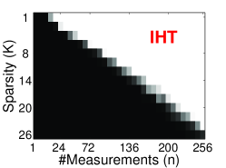
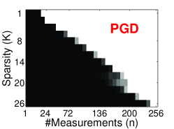
Refer to caption
Refer to caption
Refer to caption
Figure 1: Percentage of successful recovery under various sparsity and sample size. The values range from 00 to 100100100, where a brighter color means a higher percentage of success (the brightest blocks correspond to the value of 100100100). PGD admits a higher percentage of recovery compared to IHT because it flexibly chooses the step size and sparsity parameter. As a stochastic variant, HT-SVRG performs comparably to the batch counterpart PGD.

In Figure 2, we exemplify some of the results obtained from HT-SVRG by plotting two kinds of curves: the success of percentage against the sample size n𝑛n and that against the signal sparsity K𝐾K. In this way, one can examine the detailed values and can determine the minimum sample size for a particular sparsity. For instance, the left panel tells that to ensure that 80%percent8080\% percents of the 161616-sparse signals are recovered, we have to collect 175175175 measurements. We can also learn from the right panel that using 232232232 measurements, any signal whose sparsity is 222222 or less can be reliably recovered.

Refer to caption
Refer to caption
Figure 2: Percentage of success of HT-SVRG against the number of measurements (left) and the sparsity (right).

Based on the results in Figure 1 and Figure 2, we have an approximate estimation on the minimum requirement of the sample size which ensures accurate (or exact) recovery. Now we are to investigate how many measurements are needed to guarantee a success percentage of 95%percent9595\% and 99%percent9999\%. To this end, for each signal sparsity K𝐾K, we look for the number of measurements n0subscript𝑛0n_{0} from Figure 1 where 909090 percents of success are achieved. Then we carefully enlarge n0subscript𝑛0n_{0} with step size 111 and run the algorithms. The empirical results are recorded in Figure 3, where the circle markers represent the empirical results with different colors indicating different algorithms, e.g., red circle for empirical observation of HT-SVRG. Then we fit these empirical results by linear regression, which are plotted as solid or dashed lines. For example, the green line is a fitted model for IHT. We find that n𝑛n is almost linear with K𝐾K. Especially, the curve of HT-SVRG is nearly on top of that of PGD, which again verifies HT-SVRG is an attractive alternative to the batch method.
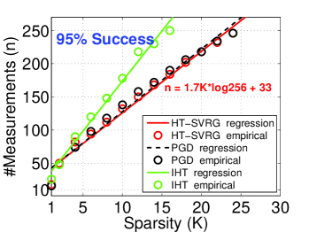
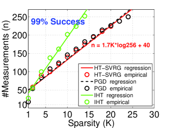
Refer to caption
Refer to caption
Figure 3: Minimum number of measurements to achieve 95%percent9595\% and 99%percent9999\% percentage of success. Red equation indicates the linear regression of HT-SVRG. The markers and curves for HT-SVRG are almost on top of PGD, which again justifies that HT-SVRG is an appealing stochastic alternative to the batch method PGD.

5.1.2 Influence of Hyper-Parameters

Next, we turn to investigate the influence of the hyper-parameters, i.e., the sparsity parameter k𝑘k, update frequency m𝑚m and step size η𝜂\eta on the convergence behavior of HT-SVRG. We set the true sparsity K=4𝐾4K=4 and collect 100100100 measurements for each groundtruth signal, i.e., n=100𝑛100n=100. Note that the standard setting we employed is k=9K=36𝑘9𝐾36k=9K=36, m=3n=300𝑚3𝑛300m=3n=300 and η=2/svds(𝑨𝑨)0.3𝜂2svds𝑨superscript𝑨top0.3\eta=2/\mathrm{svds}(\boldsymbol{A}\boldsymbol{A}^{\top})\approx 0.3. Each time we vary one of these parameters while fixing the other two, and the results are plotted in Figure 4. We point out that although the convergence result (Theorem 10) is deterministic, the vanishing optimization error (Proposition 18) is guaranteed under a probabilistic argument. Hence, it is possible that for a specific configuration of parameters, 97%percent9797\% of the signals are exactly recovered but HT-SVRG fails on the remaining, as we have observed in, e.g., Figure 2. Clearly, we are not supposed to average all the results to examine the convergence rate. For our purpose, we set a threshold 95%percent9595\%, that is, we average over the success trials if more than 95%percent9595\% percents of the signals are exactly recovered. Otherwise, we say that the set of parameters cannot ensure convergence and we average over these failure signals which will give an illustration of divergence.
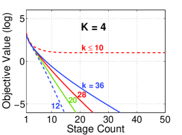
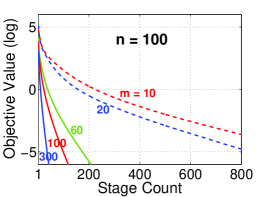
Refer to caption
Refer to caption
Refer to caption
Figure 4: Convergence of HT-SVRG with different parameters. We have 100100100 measurements for the 256256256-dimensional signal where only 444 elements are non-zero. The standard setting is k=36𝑘36k=36, m=300𝑚300m=300 and η=0.3𝜂0.3\eta=0.3. Left: If the sparsity parameter k𝑘k is not large enough, HT-SVRG will not recover the signal. Middle: A small m𝑚m leads to a frequent full gradient evaluation and hence slow convergence. Right: We observe divergence when η3𝜂3\eta\geq 3.

The left panel of Figure 4 verifies the condition that k𝑘k has to be larger than K𝐾K, while the second panel shows the update frequency m𝑚m can be reasonably small in the price of a slow convergence rate. Finally, the empirical study demonstrates that our heuristic choice η=0.3𝜂0.3\eta=0.3 works well, and when η>3𝜂3\eta>3, the objective value exceeds 10120superscript1012010^{120} within 3 stages (which cannot be depicted in the figure). For very small step sizes, we plot the convergence curve by gradually enlarging the update frequency m𝑚m in Figure 5. The empirical results agree with Theorem 10 that for any 0<η<1/(4L)0𝜂14𝐿0<\eta<1/(4L), HT-SVRG converges as soon as m𝑚m is large enough.

Refer to caption
Refer to caption
Refer to caption
Figure 5: Convergence behavior under small step size. We observe that as long as we pick a sufficiently large value for m𝑚m, HT-SVRG always converges. This is not surprising since our theorem guarantees for any η<1/(4L)𝜂14𝐿\eta<1/(4L), HT-SVRG will converge if m𝑚m is large enough. Also note that the geometric convergence rate is observed after certain iterations, e.g., for η=3×10⁵𝜂3superscript105\eta=3\times 10^{-5}, the log(error) decreases linearly after 20 thousands iterations.

5.2 Classification

In addition to the application of sparse recovery, we illustrated that HT-SVRG can deal with binary classification by minimizing the sparse logistic regression problem (4.10). Here, we study the performance on a realistic image dataset MNIST111http://yann.lecun.com/exdb/mnist/, consisting of 60 thousands training samples and 10 thousands samples for testing. There is one digit on each image of size 28-by-28, hence totally 10 classes. Some of the images are shown in Figure 6.
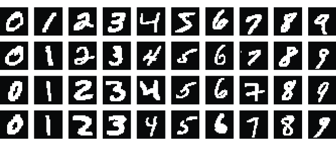
Refer to caption
Figure 6: Sample images in the MNIST database.

The update frequency m𝑚m is fixed as m=3n𝑚3𝑛m=3n. We compute the heuristic step size η𝜂\eta as in the previous section, i.e., η=2/svds(𝑨𝑨)103𝜂2svds𝑨superscript𝑨topsuperscript103\eta=2/\mathrm{svds}(\boldsymbol{A}\boldsymbol{A}^{\top})\approx 10^{-3}. Since for the real-world dataset, the true sparsity is actually unknown, we tune the sparsity parameter k𝑘k and study the performance of the algorithm.

First, we visualize five pair-wise models learned by HT-SVRG in Figure 7, where each row is associated with a binary classification task indicated by the two digits at the leading of the row, and the subsequent red-blue figures are used to illustrate the learned models under different sparsity parameter. For example, the third colorful figure depicted on the second row corresponds to recognizing a digit is “1” or “7” with the sparsity k=30𝑘30k=30. In particular, for each pair, we label the small digit as positive and the large one as negative, and the blue and red pixels are the weights with positive and negative values respectively. Apparently, the models we learned are discriminative.
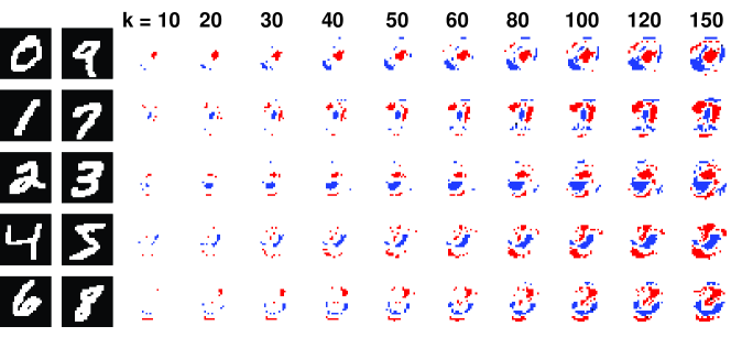
Refer to caption
Figure 7: Visualization of the models. We visualize 5 models learned by HT-SVRG under different choices of sparsity shown on the top of each column. Note that the feature dimension is 784. From the top row to the bottom row, we illustrate the models of “0 vs 9”, “1 vs 7”, “2 vs 3”, “4 vs 5” and “6 vs 8”, where for each pair, we label the small digit as positive and the large one as negative. The red color represents negative weights while the blue pixels correspond with positive weights.

We also quantitatively show the convergence and prediction accuracy curves in Figure 8. Note that here, the y𝑦y-axis is the objective value F(𝒙~s)𝐹superscript~𝒙𝑠F(\widetilde{\boldsymbol{x}}^{s}) rather than log(F(𝒙~s)F(𝒙opt))𝐹superscript~𝒙𝑠𝐹subscript𝒙opt\log(F(\widetilde{\boldsymbol{x}}^{s})-F(\boldsymbol{x}_{\mathrm{opt}})), due to the fact that computing the exact optimum of (4.10) is NP-hard. Generally speaking, HT-SVRG converges quite fast and usually attains the minimum of objective value within 20 stages. It is not surprising to see that choosing a large quantity for the sparsity leads to a better (lower) objective value. However, in practice a small assignment for the sparsity, e.g., k=70𝑘70k=70 facilitates an efficient computation while still suffices to ensure fast convergence and accurate prediction.
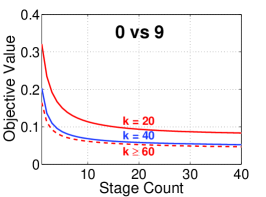
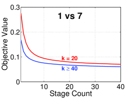
Refer to caption
Refer to caption
Refer to caption
Refer to caption
Refer to caption
Refer to caption
Figure 8: Quantitative results on convergence and accuracy. The first 5 figures demonstrate the convergence behavior of HT-SVRG for each binary classification task, where curves with different colors represent the objective value against number of stages under different sparsity k𝑘k. Generally speaking, HT-SVRG converges within 20 stages which is a very fast rate. The last figure reflects the classification accuracy against the sparsity for all 5 classification tasks, where we find that for a moderate choice, e.g., k=70𝑘70k=70, it already guarantees an accurate prediction (we recall the dimension is 784).

6 Conclusion and Open Problems

In this paper, we have provided a tight bound on the deviation resulting from the hard thresholding operator, which underlies a vast volume of algorithms developed for sparsity-constrained problems. Our derived bound is universal over all choices of parameters and we have proved that it cannot be improved without further information on the signals. We have discussed the implications of our result to the community of compressed sensing and machine learning, and have demonstrated that the theoretical results of a number of popular algorithms in the literature can be advanced. In addition, we have devised a novel algorithm which tackles the problem of sparse learning in large-scale setting. We have elaborated that our algorithm is guaranteed to produce global optimal solution for prevalent statistical models only when it is equipped with the tight bound, hence justifying that the conventional bound is not applicable in the challenging scenario.

There are several interesting open problems. The first question to ask is whether one can establish sharp RIP condition or sharp phase transition for hard thresholding based algorithms such as IHT and CoSaMP with the tight bound. Moreover, compared to the hard thresholded SGD method [NNW14], HT-SVRG admits a vanishing optimization error. This poses a question of whether we are able to provably show the necessity of variance reduction for such a sparsity-constrained problem.

Acknowledgments

We would like to thank Jing Wang for insightful discussion since the early stage of the work. We also thank Martin Slawski for helpful discussion on the statistical precision of the problem, and thank Jian Wang for bringing the paper [NNW14] into our attention. We appreciate Huan Xu’s high level comments on the work. Finally, we thank the anonymous reviewers for a careful check on our proof and for the encouraging comments. The work was partially funded by NSF-Bigdata-1419210 and NSF-III-1360971.

Appendix A Technical Lemmas

We present some useful lemmas that will be invoked by subsequent analysis. The following is a characterization of the co-coercivity of the objective function F(𝒙)𝐹𝒙F(\boldsymbol{x}). A similar result was obtained in [NNW14] but we present a refined analysis which is essential for our purpose.

Lemma 19.

For a given support set ΩΩ\Omega, assume that the continuous function F(𝐱)𝐹𝐱F(\boldsymbol{x}) is L|Ω|subscript𝐿ΩL_{\left\lvert\Omega\right\rvert}-RSS and is αKsubscript𝛼𝐾\alpha_{K}-RSC for some sparsity level K𝐾K. Then, for all vectors 𝐱𝐱\boldsymbol{x} and 𝐱superscript𝐱\boldsymbol{x}^{\prime} with |supp(𝐱𝐱)Ω|Ksupp𝐱superscript𝐱Ω𝐾\left\lvert\mathrm{supp}\left(\boldsymbol{x}-\boldsymbol{x}^{\prime}\right)\cup\Omega\right\rvert\leq K,

ΩF(𝒙)ΩF(𝒙)222L|Ω|(F(𝒙)F(𝒙)F(𝒙),𝒙𝒙).superscriptsubscriptdelimited-∥∥subscriptΩ𝐹superscript𝒙subscriptΩ𝐹𝒙222subscript𝐿Ω𝐹superscript𝒙𝐹𝒙𝐹𝒙superscript𝒙𝒙\left\lVert\nabla_{\Omega}F(\boldsymbol{x}^{\prime})-\nabla_{\Omega}F(\boldsymbol{x})\right\rVert_{2}^{2}\leq 2L_{\left\lvert\Omega\right\rvert}\big{(}F(\boldsymbol{x}^{\prime})-F(\boldsymbol{x})-\left\langle\nabla F(\boldsymbol{x}),\boldsymbol{x}^{\prime}-\boldsymbol{x}\right\rangle\big{)}.
Proof.

We define an auxiliary function

G(𝒘):=F(𝒘)F(𝒙),𝒘.assign𝐺𝒘𝐹𝒘𝐹𝒙𝒘G(\boldsymbol{w}):=F(\boldsymbol{w})-\left\langle\nabla F(\boldsymbol{x}),\boldsymbol{w}\right\rangle.

For all vectors 𝒘𝒘\boldsymbol{w} and 𝒘superscript𝒘\boldsymbol{w}^{\prime}, we have

G(𝒘)G(𝒘)2=F(𝒘)F(𝒘)2L|supp(𝒘𝒘)|𝒘𝒘2,subscriptdelimited-∥∥𝐺𝒘𝐺superscript𝒘2subscriptdelimited-∥∥𝐹𝒘𝐹superscript𝒘2subscript𝐿supp𝒘superscript𝒘subscriptdelimited-∥∥𝒘superscript𝒘2\left\lVert\nabla G(\boldsymbol{w})-\nabla G(\boldsymbol{w}^{\prime})\right\rVert_{2}=\left\lVert\nabla F(\boldsymbol{w})-\nabla F(\boldsymbol{w}^{\prime})\right\rVert_{2}\leq L_{\left\lvert\mathrm{supp}\left(\boldsymbol{w}-\boldsymbol{w}^{\prime}\right)\right\rvert}\left\lVert\boldsymbol{w}-\boldsymbol{w}^{\prime}\right\rVert_{2},

which is equivalent to

G(𝒘)G(𝒘)G(𝒘),𝒘𝒘Lr2𝒘𝒘22,𝐺𝒘𝐺superscript𝒘𝐺superscript𝒘𝒘superscript𝒘subscript𝐿𝑟2superscriptsubscriptdelimited-∥∥𝒘superscript𝒘22G(\boldsymbol{w})-G(\boldsymbol{w}^{\prime})-\left\langle\nabla G(\boldsymbol{w}^{\prime}),\boldsymbol{w}-\boldsymbol{w}^{\prime}\right\rangle\leq\frac{L_{r}}{2}\left\lVert\boldsymbol{w}-\boldsymbol{w}^{\prime}\right\rVert_{2}^{2}, (A.1)

where r:=|supp(𝒘𝒘)|assign𝑟supp𝒘superscript𝒘r:=\left\lvert\mathrm{supp}\left(\boldsymbol{w}-\boldsymbol{w}^{\prime}\right)\right\rvert. On the other hand, due to the RSC property of F(𝒙)𝐹𝒙F(\boldsymbol{x}), we obtain

G(𝒘)G(𝒙)=F(𝒘)F(𝒙)F(𝒙),𝒘𝒙α|supp(𝒘𝒙)|2𝒘𝒙220,𝐺𝒘𝐺𝒙𝐹𝒘𝐹𝒙𝐹𝒙𝒘𝒙subscript𝛼supp𝒘𝒙2superscriptsubscriptdelimited-∥∥𝒘𝒙220G(\boldsymbol{w})-G(\boldsymbol{x})=F(\boldsymbol{w})-F(\boldsymbol{x})-\left\langle\nabla F(\boldsymbol{x}),\boldsymbol{w}-\boldsymbol{x}\right\rangle\geq\frac{\alpha_{\left\lvert\mathrm{supp}\left(\boldsymbol{w}-\boldsymbol{x}\right)\right\rvert}}{2}\left\lVert\boldsymbol{w}-\boldsymbol{x}\right\rVert_{2}^{2}\geq 0,

provided that |supp(𝒘𝒙)|Ksupp𝒘𝒙𝐾\left\lvert\mathrm{supp}\left(\boldsymbol{w}-\boldsymbol{x}\right)\right\rvert\leq K. For the given support set ΩΩ\Omega, we pick 𝒘=𝒙1L|Ω|ΩG(𝒙)𝒘superscript𝒙1subscript𝐿ΩsubscriptΩ𝐺superscript𝒙\boldsymbol{w}=\boldsymbol{x}^{\prime}-\frac{1}{L_{\left\lvert\Omega\right\rvert}}\nabla_{\Omega}G(\boldsymbol{x}^{\prime}). Clearly, for such a choice of 𝒘𝒘\boldsymbol{w}, we have supp(𝒘𝒙)=supp(𝒙𝒙)Ωsupp𝒘𝒙supp𝒙superscript𝒙Ω{\mathrm{supp}\left(\boldsymbol{w}-\boldsymbol{x}\right)}=\mathrm{supp}\left(\boldsymbol{x}-\boldsymbol{x}^{\prime}\right)\cup\Omega. Hence, by assuming that |supp(𝒙𝒙)Ω|supp𝒙superscript𝒙Ω\left\lvert\mathrm{supp}\left(\boldsymbol{x}-\boldsymbol{x}^{\prime}\right)\cup\Omega\right\rvert is not larger than K𝐾K, we get

G(𝒙)𝐺𝒙absent\displaystyle G(\boldsymbol{x})\leq G(𝒙1L|Ω|ΩG(𝒙))𝐺superscript𝒙1subscript𝐿ΩsubscriptΩ𝐺superscript𝒙\displaystyle\ G\left(\boldsymbol{x}^{\prime}-\frac{1}{L_{\left\lvert\Omega\right\rvert}}\nabla_{\Omega}G(\boldsymbol{x}^{\prime})\right)
\displaystyle{\leq} G(𝒙)+G(𝒙),1L|Ω|ΩG(𝒙)+12L|Ω|ΩG(𝒙)22𝐺superscript𝒙𝐺superscript𝒙1subscript𝐿ΩsubscriptΩ𝐺superscript𝒙12subscript𝐿Ωsuperscriptsubscriptdelimited-∥∥subscriptΩ𝐺superscript𝒙22\displaystyle\ G(\boldsymbol{x}^{\prime})+\left\langle\nabla G(\boldsymbol{x}^{\prime}),-\frac{1}{L_{\left\lvert\Omega\right\rvert}}\nabla_{\Omega}G(\boldsymbol{x}^{\prime})\right\rangle+\frac{1}{2L_{\left\lvert\Omega\right\rvert}}\left\lVert\nabla_{\Omega}G(\boldsymbol{x}^{\prime})\right\rVert_{2}^{2}
=\displaystyle= G(𝒙)12L|Ω|ΩG(𝒙)22,𝐺superscript𝒙12subscript𝐿Ωsuperscriptsubscriptdelimited-∥∥subscriptΩ𝐺superscript𝒙22\displaystyle\ G(\boldsymbol{x}^{\prime})-\frac{1}{2L_{\left\lvert\Omega\right\rvert}}\left\lVert\nabla_{\Omega}G(\boldsymbol{x}^{\prime})\right\rVert_{2}^{2},

where the second inequality follows from (A.1). Now expanding ΩG(𝒙)subscriptΩ𝐺superscript𝒙\nabla_{\Omega}G(\boldsymbol{x}^{\prime}) and rearranging the terms gives the desired result. ∎

Lemma 20.

Consider the HT-SVRG algorithm for a fixed stage s𝑠s. Let 𝐱^^𝐱\widehat{\boldsymbol{x}} be the target sparse vector. Let ΩΩ\Omega be a support set such that supp(𝐱t1)supp(𝐱~)supp(𝐱^)Ωsuppsuperscript𝐱𝑡1supp~𝐱supp^𝐱Ω\mathrm{supp}\left(\boldsymbol{x}^{t-1}\right)\cup\mathrm{supp}\left(\widetilde{\boldsymbol{x}}\right)\cup\mathrm{supp}\left(\widehat{\boldsymbol{x}}\right)\subseteq\Omega. Put r=|Ω|𝑟Ωr=\left\lvert\Omega\right\rvert. Assume (A2)𝐴2(A2). For all 1tm1𝑡𝑚1\leq t\leq m , denote 𝐯t=fit(𝐱t1)fit(𝐱~)+𝛍~superscript𝐯𝑡subscript𝑓subscript𝑖𝑡superscript𝐱𝑡1subscript𝑓subscript𝑖𝑡~𝐱~𝛍\boldsymbol{v}^{t}=\nabla f_{i_{t}}(\boldsymbol{x}^{t-1})-\nabla f_{i_{t}}(\widetilde{\boldsymbol{x}})+\widetilde{\boldsymbol{\mu}}. Then we have the following:

𝔼it|𝒙t1[𝒫Ω(𝒗t)22]subscript𝔼conditionalsubscript𝑖𝑡superscript𝒙𝑡1superscriptsubscriptdelimited-∥∥subscript𝒫Ωsuperscript𝒗𝑡22absent\displaystyle{\operatorname*{\mathbb{E}}}_{i_{t}|\boldsymbol{x}^{t-1}}\Big{[}\left\lVert\mathcal{P}_{\Omega}\left(\boldsymbol{v}^{t}\right)\right\rVert_{2}^{2}\Big{]}\leq 4Lr[F(𝒙t1)F(𝒙^)]+4Lr[F(𝒙~)F(𝒙^)]4subscript𝐿𝑟delimited-[]𝐹superscript𝒙𝑡1𝐹^𝒙4subscript𝐿𝑟delimited-[]𝐹~𝒙𝐹^𝒙\displaystyle\ 4L_{r}\left[F(\boldsymbol{x}^{t-1})-F(\widehat{\boldsymbol{x}})\right]+4L_{r}\left[F(\widetilde{\boldsymbol{x}})-F(\widehat{\boldsymbol{x}})\right]
4LrF(𝒙^),𝒙t1+𝒙~2𝒙^+4𝒫Ω(F(𝒙^))22.4subscript𝐿𝑟𝐹^𝒙superscript𝒙𝑡1~𝒙2^𝒙4superscriptsubscriptdelimited-∥∥subscript𝒫Ω𝐹^𝒙22\displaystyle\ -4L_{r}\left\langle\nabla F(\widehat{\boldsymbol{x}}),\boldsymbol{x}^{t-1}+\widetilde{\boldsymbol{x}}-2\widehat{\boldsymbol{x}}\right\rangle+4\left\lVert\mathcal{P}_{\Omega}\left(\nabla F(\widehat{\boldsymbol{x}})\right)\right\rVert_{2}^{2}.
Proof.

We have

𝒫Ω(𝒗t)22=superscriptsubscriptdelimited-∥∥subscript𝒫Ωsuperscript𝒗𝑡22absent\displaystyle\left\lVert\mathcal{P}_{\Omega}\left(\boldsymbol{v}^{t}\right)\right\rVert_{2}^{2}= 𝒫Ω(fit(𝒙t1)fit(𝒙~)+𝝁~)22superscriptsubscriptdelimited-∥∥subscript𝒫Ωsubscript𝑓subscript𝑖𝑡superscript𝒙𝑡1subscript𝑓subscript𝑖𝑡~𝒙~𝝁22\displaystyle\ \left\lVert\mathcal{P}_{\Omega}\left(\nabla f_{i_{t}}(\boldsymbol{x}^{t-1})-\nabla f_{i_{t}}(\widetilde{\boldsymbol{x}})+\widetilde{\boldsymbol{\mu}}\right)\right\rVert_{2}^{2}
\displaystyle\leq 2𝒫Ω(fit(𝒙t1)fit(𝒙^))22+2𝒫Ω(fit(𝒙~)fit(𝒙^)𝝁~)222superscriptsubscriptdelimited-∥∥subscript𝒫Ωsubscript𝑓subscript𝑖𝑡superscript𝒙𝑡1subscript𝑓subscript𝑖𝑡^𝒙222superscriptsubscriptdelimited-∥∥subscript𝒫Ωsubscript𝑓subscript𝑖𝑡~𝒙subscript𝑓subscript𝑖𝑡^𝒙~𝝁22\displaystyle\ 2\left\lVert\mathcal{P}_{\Omega}\left(\nabla f_{i_{t}}(\boldsymbol{x}^{t-1})-\nabla f_{i_{t}}(\widehat{\boldsymbol{x}})\right)\right\rVert_{2}^{2}+2\left\lVert\mathcal{P}_{\Omega}\left(\nabla f_{i_{t}}(\widetilde{\boldsymbol{x}})-\nabla f_{i_{t}}(\widehat{\boldsymbol{x}})-\widetilde{\boldsymbol{\mu}}\right)\right\rVert_{2}^{2}
=\displaystyle= 2𝒫Ω(fit(𝒙t1)fit(𝒙^))22+2𝒫Ω(fit(𝒙~)fit(𝒙^))222superscriptsubscriptdelimited-∥∥subscript𝒫Ωsubscript𝑓subscript𝑖𝑡superscript𝒙𝑡1subscript𝑓subscript𝑖𝑡^𝒙222superscriptsubscriptdelimited-∥∥subscript𝒫Ωsubscript𝑓subscript𝑖𝑡~𝒙subscript𝑓subscript𝑖𝑡^𝒙22\displaystyle\ 2\left\lVert\mathcal{P}_{\Omega}\left(\nabla f_{i_{t}}(\boldsymbol{x}^{t-1})-\nabla f_{i_{t}}(\widehat{\boldsymbol{x}})\right)\right\rVert_{2}^{2}+2\left\lVert\mathcal{P}_{\Omega}\left(\nabla f_{i_{t}}(\widetilde{\boldsymbol{x}})-\nabla f_{i_{t}}(\widehat{\boldsymbol{x}})\right)\right\rVert_{2}^{2}
+2𝒫Ω(𝝁~)224𝒫Ω(fit(𝒙~)fit(𝒙^)),𝒫Ω(𝝁~)2superscriptsubscriptdelimited-∥∥subscript𝒫Ω~𝝁224subscript𝒫Ωsubscript𝑓subscript𝑖𝑡~𝒙subscript𝑓subscript𝑖𝑡^𝒙subscript𝒫Ω~𝝁\displaystyle\ +2\left\lVert\mathcal{P}_{\Omega}\left(\widetilde{\boldsymbol{\mu}}\right)\right\rVert_{2}^{2}-4\left\langle\mathcal{P}_{\Omega}\left(\nabla f_{i_{t}}(\widetilde{\boldsymbol{x}})-\nabla f_{i_{t}}(\widehat{\boldsymbol{x}})\right),\mathcal{P}_{\Omega}\left(\widetilde{\boldsymbol{\mu}}\right)\right\rangle
=ξ1superscriptsubscript𝜉1\displaystyle\stackrel{{\scriptstyle\xi_{1}}}{{=}} 2𝒫Ω(fit(𝒙t1)fit(𝒙^))22+2𝒫Ω(fit(𝒙~)fit(𝒙^))222superscriptsubscriptdelimited-∥∥subscript𝒫Ωsubscript𝑓subscript𝑖𝑡superscript𝒙𝑡1subscript𝑓subscript𝑖𝑡^𝒙222superscriptsubscriptdelimited-∥∥subscript𝒫Ωsubscript𝑓subscript𝑖𝑡~𝒙subscript𝑓subscript𝑖𝑡^𝒙22\displaystyle\ 2\left\lVert\mathcal{P}_{\Omega}\left(\nabla f_{i_{t}}(\boldsymbol{x}^{t-1})-\nabla f_{i_{t}}(\widehat{\boldsymbol{x}})\right)\right\rVert_{2}^{2}+2\left\lVert\mathcal{P}_{\Omega}\left(\nabla f_{i_{t}}(\widetilde{\boldsymbol{x}})-\nabla f_{i_{t}}(\widehat{\boldsymbol{x}})\right)\right\rVert_{2}^{2}
+2𝒫Ω(𝝁~)224fit(𝒙~)fit(𝒙^),𝒫Ω(𝝁~)2superscriptsubscriptdelimited-∥∥subscript𝒫Ω~𝝁224subscript𝑓subscript𝑖𝑡~𝒙subscript𝑓subscript𝑖𝑡^𝒙subscript𝒫Ω~𝝁\displaystyle\ +2\left\lVert\mathcal{P}_{\Omega}\left(\widetilde{\boldsymbol{\mu}}\right)\right\rVert_{2}^{2}-4\left\langle{\nabla f_{i_{t}}(\widetilde{\boldsymbol{x}})-\nabla f_{i_{t}}(\widehat{\boldsymbol{x}})},\mathcal{P}_{\Omega}\left(\widetilde{\boldsymbol{\mu}}\right)\right\rangle
ξ2superscriptsubscript𝜉2\displaystyle\stackrel{{\scriptstyle\xi_{2}}}{{\leq}} 4Lr[fit(𝒙t1)fit(𝒙^)fit(𝒙^),𝒙t1𝒙^]4subscript𝐿𝑟delimited-[]subscript𝑓subscript𝑖𝑡superscript𝒙𝑡1subscript𝑓subscript𝑖𝑡^𝒙subscript𝑓subscript𝑖𝑡^𝒙superscript𝒙𝑡1^𝒙\displaystyle\ 4L_{r}\left[f_{i_{t}}(\boldsymbol{x}^{t-1})-f_{i_{t}}(\widehat{\boldsymbol{x}})-\left\langle\nabla f_{i_{t}}(\widehat{\boldsymbol{x}}),\boldsymbol{x}^{t-1}-\widehat{\boldsymbol{x}}\right\rangle\right]
+4Lr[fit(𝒙~)fit(𝒙^)fit(𝒙^),𝒙~𝒙^]4subscript𝐿𝑟delimited-[]subscript𝑓subscript𝑖𝑡~𝒙subscript𝑓subscript𝑖𝑡^𝒙subscript𝑓subscript𝑖𝑡^𝒙~𝒙^𝒙\displaystyle\ +4L_{r}\left[f_{i_{t}}(\widetilde{\boldsymbol{x}})-f_{i_{t}}(\widehat{\boldsymbol{x}})-\left\langle\nabla f_{i_{t}}(\widehat{\boldsymbol{x}}),\widetilde{\boldsymbol{x}}-\widehat{\boldsymbol{x}}\right\rangle\right]
+2𝒫Ω(𝝁~)224fit(𝒙~)fit(𝒙^),𝒫Ω(𝝁~),2superscriptsubscriptdelimited-∥∥subscript𝒫Ω~𝝁224subscript𝑓subscript𝑖𝑡~𝒙subscript𝑓subscript𝑖𝑡^𝒙subscript𝒫Ω~𝝁\displaystyle\ +2\left\lVert\mathcal{P}_{\Omega}\left(\widetilde{\boldsymbol{\mu}}\right)\right\rVert_{2}^{2}-4\left\langle{\nabla f_{i_{t}}(\widetilde{\boldsymbol{x}})-\nabla f_{i_{t}}(\widehat{\boldsymbol{x}})},\mathcal{P}_{\Omega}\left(\widetilde{\boldsymbol{\mu}}\right)\right\rangle,

where ξ1subscript𝜉1\xi_{1} is by algebra, ξ2subscript𝜉2\xi_{2} applies Lemma 19 and the fact that |Ω|=rΩ𝑟\left\lvert\Omega\right\rvert=r.

Taking the conditional expectation, we obtain the following:

𝔼it|𝒙t1[𝒫Ω(𝒗t)22]subscript𝔼conditionalsubscript𝑖𝑡superscript𝒙𝑡1superscriptsubscriptdelimited-∥∥subscript𝒫Ωsuperscript𝒗𝑡22\displaystyle\ {\operatorname*{\mathbb{E}}}_{i_{t}|\boldsymbol{x}^{t-1}}\Big{[}\left\lVert\mathcal{P}_{\Omega}\left(\boldsymbol{v}^{t}\right)\right\rVert_{2}^{2}\Big{]}
\displaystyle\leq 4Lr[F(𝒙t1)F(𝒙^)]+4Lr[F(𝒙~)F(𝒙^)]4subscript𝐿𝑟delimited-[]𝐹superscript𝒙𝑡1𝐹^𝒙4subscript𝐿𝑟delimited-[]𝐹~𝒙𝐹^𝒙\displaystyle\ 4L_{r}\left[F(\boldsymbol{x}^{t-1})-F(\widehat{\boldsymbol{x}})\right]+4L_{r}\left[F(\widetilde{\boldsymbol{x}})-F(\widehat{\boldsymbol{x}})\right]
4LrF(𝒙^),𝒙t1+𝒙~2𝒙^+22𝒫Ω(F(𝒙^))𝒫Ω(𝝁~),𝒫Ω(𝝁~)4subscript𝐿𝑟𝐹^𝒙superscript𝒙𝑡1~𝒙2^𝒙22subscript𝒫Ω𝐹^𝒙subscript𝒫Ω~𝝁subscript𝒫Ω~𝝁\displaystyle\ -4L_{r}\left\langle\nabla F(\widehat{\boldsymbol{x}}),\boldsymbol{x}^{t-1}+\widetilde{\boldsymbol{x}}-2\widehat{\boldsymbol{x}}\right\rangle+2\left\langle 2\mathcal{P}_{\Omega}\left(\nabla F(\widehat{\boldsymbol{x}})\right)-\mathcal{P}_{\Omega}\left(\widetilde{\boldsymbol{\mu}}\right),\mathcal{P}_{\Omega}\left(\widetilde{\boldsymbol{\mu}}\right)\right\rangle
=\displaystyle= 4Lr[F(𝒙t1)F(𝒙^)]+4Lr[F(𝒙~)F(𝒙^)]4subscript𝐿𝑟delimited-[]𝐹superscript𝒙𝑡1𝐹^𝒙4subscript𝐿𝑟delimited-[]𝐹~𝒙𝐹^𝒙\displaystyle\ 4L_{r}\left[F(\boldsymbol{x}^{t-1})-F(\widehat{\boldsymbol{x}})\right]+4L_{r}\left[F(\widetilde{\boldsymbol{x}})-F(\widehat{\boldsymbol{x}})\right]
4LrF(𝒙^),𝒙t1+𝒙~2𝒙^+2𝒫Ω(F(𝒙^))224subscript𝐿𝑟𝐹^𝒙superscript𝒙𝑡1~𝒙2^𝒙superscriptsubscriptdelimited-∥∥2subscript𝒫Ω𝐹^𝒙22\displaystyle\ -4L_{r}\left\langle\nabla F(\widehat{\boldsymbol{x}}),\boldsymbol{x}^{t-1}+\widetilde{\boldsymbol{x}}-2\widehat{\boldsymbol{x}}\right\rangle+\left\lVert 2\mathcal{P}_{\Omega}\left(\nabla F(\widehat{\boldsymbol{x}})\right)\right\rVert_{2}^{2}
2𝒫Ω(F(𝒙^))𝒫Ω(𝝁~)22𝒫Ω(𝝁~)22superscriptsubscriptdelimited-∥∥2subscript𝒫Ω𝐹^𝒙subscript𝒫Ω~𝝁22superscriptsubscriptdelimited-∥∥subscript𝒫Ω~𝝁22\displaystyle\ -\left\lVert 2\mathcal{P}_{\Omega}\left(\nabla F(\widehat{\boldsymbol{x}})\right)-\mathcal{P}_{\Omega}\left(\widetilde{\boldsymbol{\mu}}\right)\right\rVert_{2}^{2}-\left\lVert\mathcal{P}_{\Omega}\left(\widetilde{\boldsymbol{\mu}}\right)\right\rVert_{2}^{2}
\displaystyle\leq 4Lr[F(𝒙t1)F(𝒙^)]+4Lr[F(𝒙~)F(𝒙^)]4subscript𝐿𝑟delimited-[]𝐹superscript𝒙𝑡1𝐹^𝒙4subscript𝐿𝑟delimited-[]𝐹~𝒙𝐹^𝒙\displaystyle\ 4L_{r}\left[F(\boldsymbol{x}^{t-1})-F(\widehat{\boldsymbol{x}})\right]+4L_{r}\left[F(\widetilde{\boldsymbol{x}})-F(\widehat{\boldsymbol{x}})\right]
4LrF(𝒙^),𝒙t1+𝒙~2𝒙^+4𝒫Ω(F(𝒙^))22.4subscript𝐿𝑟𝐹^𝒙superscript𝒙𝑡1~𝒙2^𝒙4superscriptsubscriptdelimited-∥∥subscript𝒫Ω𝐹^𝒙22\displaystyle\ -4L_{r}\left\langle\nabla F(\widehat{\boldsymbol{x}}),\boldsymbol{x}^{t-1}+\widetilde{\boldsymbol{x}}-2\widehat{\boldsymbol{x}}\right\rangle+4\left\lVert\mathcal{P}_{\Omega}\left(\nabla F(\widehat{\boldsymbol{x}})\right)\right\rVert_{2}^{2}.

The proof is complete. ∎

Corollary 21.

Assume the same conditions as in Lemma 20. If F(𝐱^)=0𝐹^𝐱0\nabla F(\widehat{\boldsymbol{x}})=0, we have

𝔼it|𝒙t1[𝒫Ω(𝒗t)22]4Lr[F(𝒙t1)+F(𝒙~)2F(𝒙^)].subscript𝔼conditionalsubscript𝑖𝑡superscript𝒙𝑡1superscriptsubscriptdelimited-∥∥subscript𝒫Ωsuperscript𝒗𝑡224subscript𝐿𝑟delimited-[]𝐹superscript𝒙𝑡1𝐹~𝒙2𝐹^𝒙{\operatorname*{\mathbb{E}}}_{i_{t}|\boldsymbol{x}^{t-1}}\Big{[}\left\lVert\mathcal{P}_{\Omega}\left(\boldsymbol{v}^{t}\right)\right\rVert_{2}^{2}\Big{]}\leq 4L_{r}\left[F(\boldsymbol{x}^{t-1})+F(\widetilde{\boldsymbol{x}})-2F(\widehat{\boldsymbol{x}})\right].

Appendix B Proofs for Section 2

B.1 Proof of Theorem 1

Proof.

The result is true for the trivial case that 𝒃𝒃\boldsymbol{b} is a zero vector. In the following, we assume that 𝒃𝒃\boldsymbol{b} is not a zero vector. Denote

𝒘:=k(𝒃).assign𝒘subscript𝑘𝒃\boldsymbol{w}:=\mathcal{H}_{k}\left(\boldsymbol{b}\right).

Let ΩΩ\Omega be the support set of 𝒘𝒘\boldsymbol{w} and let Ω¯¯Ω\overline{\Omega} be its complement. We immediately have 𝒫Ω(𝒃)=𝒘subscript𝒫Ω𝒃𝒘\mathcal{P}_{\Omega}\left(\boldsymbol{b}\right)=\boldsymbol{w}.

Let ΩsuperscriptΩ\Omega^{\prime} be the support set of 𝒙𝒙\boldsymbol{x}. For the sake of simplicity, let us split the vector 𝒃𝒃\boldsymbol{b} as follows:

𝒃1=𝒫Ω\Ω(𝒃),subscript𝒃1subscript𝒫\ΩsuperscriptΩ𝒃\displaystyle\boldsymbol{b}_{1}=\mathcal{P}_{\Omega\backslash\Omega^{\prime}}\left(\boldsymbol{b}\right),\quad 𝒃2=𝒫ΩΩ(𝒃),subscript𝒃2subscript𝒫ΩsuperscriptΩ𝒃\displaystyle\boldsymbol{b}_{2}=\mathcal{P}_{\Omega\cap\Omega^{\prime}}\left(\boldsymbol{b}\right),
𝒃3=𝒫Ω¯\Ω(𝒃),subscript𝒃3subscript𝒫\¯ΩsuperscriptΩ𝒃\displaystyle\boldsymbol{b}_{3}=\mathcal{P}_{\overline{\Omega}\backslash\Omega^{\prime}}\left(\boldsymbol{b}\right),\quad 𝒃4=𝒫Ω¯Ω(𝒃).subscript𝒃4subscript𝒫¯ΩsuperscriptΩ𝒃\displaystyle\boldsymbol{b}_{4}=\mathcal{P}_{\overline{\Omega}\cap\Omega^{\prime}}\left(\boldsymbol{b}\right).

Likewise, we denote

𝒘1=𝒫Ω\Ω(𝒘),𝒘2=𝒫ΩΩ(𝒘),𝒘3=𝒫Ω¯\Ω(𝒘)=𝟎,𝒘4=𝒫Ω¯Ω(𝒘)=𝟎,formulae-sequenceformulae-sequencesubscript𝒘1subscript𝒫\ΩsuperscriptΩ𝒘formulae-sequencesubscript𝒘2subscript𝒫ΩsuperscriptΩ𝒘subscript𝒘3subscript𝒫\¯ΩsuperscriptΩ𝒘0subscript𝒘4subscript𝒫¯ΩsuperscriptΩ𝒘0\displaystyle\boldsymbol{w}_{1}=\mathcal{P}_{\Omega\backslash\Omega^{\prime}}\left(\boldsymbol{w}\right),\quad\boldsymbol{w}_{2}=\mathcal{P}_{\Omega\cap\Omega^{\prime}}\left(\boldsymbol{w}\right),\quad\boldsymbol{w}_{3}=\mathcal{P}_{\overline{\Omega}\backslash\Omega^{\prime}}(\boldsymbol{w})=\boldsymbol{0},\quad\boldsymbol{w}_{4}=\mathcal{P}_{\overline{\Omega}\cap\Omega^{\prime}}\left(\boldsymbol{w}\right)=\boldsymbol{0},
𝒙1=𝒫Ω\Ω(𝒙)=𝟎,𝒙2=𝒫ΩΩ(𝒙),𝒙3=𝒫Ω¯\Ω(𝒙)=𝟎,𝒙4=𝒫Ω¯Ω(𝒙).formulae-sequencesubscript𝒙1subscript𝒫\ΩsuperscriptΩ𝒙0formulae-sequencesubscript𝒙2subscript𝒫ΩsuperscriptΩ𝒙subscript𝒙3subscript𝒫\¯ΩsuperscriptΩ𝒙0subscript𝒙4subscript𝒫¯ΩsuperscriptΩ𝒙\displaystyle\boldsymbol{x}_{1}=\mathcal{P}_{\Omega\backslash\Omega^{\prime}}\left(\boldsymbol{x}\right)=\boldsymbol{0},\quad\boldsymbol{x}_{2}=\mathcal{P}_{\Omega\cap\Omega^{\prime}}\left(\boldsymbol{x}\right),\quad\boldsymbol{x}_{3}=\mathcal{P}_{\overline{\Omega}\backslash\Omega^{\prime}}(\boldsymbol{x})=\boldsymbol{0},\quad\boldsymbol{x}_{4}=\mathcal{P}_{\overline{\Omega}\cap\Omega^{\prime}}\left(\boldsymbol{x}\right).

Due to the hard thresholding, we have

𝒘1=𝒃1,𝒘2=𝒃2.formulae-sequencesubscript𝒘1subscript𝒃1subscript𝒘2subscript𝒃2\boldsymbol{w}_{1}=\boldsymbol{b}_{1},\quad\boldsymbol{w}_{2}=\boldsymbol{b}_{2}.

In this way, by simple algebra we have

𝒘𝒙22superscriptsubscriptdelimited-∥∥𝒘𝒙22\displaystyle\left\lVert\boldsymbol{w}-\boldsymbol{x}\right\rVert_{2}^{2} =𝒃122+𝒃2𝒙222+𝒙422,absentsuperscriptsubscriptdelimited-∥∥subscript𝒃122superscriptsubscriptdelimited-∥∥subscript𝒃2subscript𝒙222superscriptsubscriptdelimited-∥∥subscript𝒙422\displaystyle=\left\lVert\boldsymbol{b}_{1}\right\rVert_{2}^{2}+\left\lVert\boldsymbol{b}_{2}-\boldsymbol{x}_{2}\right\rVert_{2}^{2}+\left\lVert\boldsymbol{x}_{4}\right\rVert_{2}^{2},
𝒃𝒙22superscriptsubscriptdelimited-∥∥𝒃𝒙22\displaystyle\left\lVert\boldsymbol{b}-\boldsymbol{x}\right\rVert_{2}^{2} =𝒃122+𝒃2𝒙222+𝒃322+𝒃4𝒙422.absentsuperscriptsubscriptdelimited-∥∥subscript𝒃122superscriptsubscriptdelimited-∥∥subscript𝒃2subscript𝒙222superscriptsubscriptdelimited-∥∥subscript𝒃322superscriptsubscriptdelimited-∥∥subscript𝒃4subscript𝒙422\displaystyle=\left\lVert\boldsymbol{b}_{1}\right\rVert_{2}^{2}+\left\lVert\boldsymbol{b}_{2}-\boldsymbol{x}_{2}\right\rVert_{2}^{2}+\left\lVert\boldsymbol{b}_{3}\right\rVert_{2}^{2}+\left\lVert\boldsymbol{b}_{4}-\boldsymbol{x}_{4}\right\rVert_{2}^{2}.

Our goal is to estimate the maximum of 𝒘𝒙22/𝒃𝒙22superscriptsubscriptdelimited-∥∥𝒘𝒙22superscriptsubscriptdelimited-∥∥𝒃𝒙22\left\lVert\boldsymbol{w}-\boldsymbol{x}\right\rVert_{2}^{2}/\left\lVert\boldsymbol{b}-\boldsymbol{x}\right\rVert_{2}^{2}. It is easy to show that when attaining the maximum value, 𝒃32subscriptdelimited-∥∥subscript𝒃32\left\lVert\boldsymbol{b}_{3}\right\rVert_{2} must be zero since otherwise one may decrease this term to make the objective larger. Hence, maximizing 𝒘𝒙22/𝒃𝒙22superscriptsubscriptdelimited-∥∥𝒘𝒙22superscriptsubscriptdelimited-∥∥𝒃𝒙22\left\lVert\boldsymbol{w}-\boldsymbol{x}\right\rVert_{2}^{2}/\left\lVert\boldsymbol{b}-\boldsymbol{x}\right\rVert_{2}^{2} amounts to estimating the upper bound of the following over all choices of 𝒙𝒙\boldsymbol{x} and 𝒃𝒃\boldsymbol{b}:

γ:=𝒃122+𝒃2𝒙222+𝒙422𝒃122+𝒃2𝒙222+𝒃4𝒙422.assign𝛾superscriptsubscriptdelimited-∥∥subscript𝒃122superscriptsubscriptdelimited-∥∥subscript𝒃2subscript𝒙222superscriptsubscriptdelimited-∥∥subscript𝒙422superscriptsubscriptdelimited-∥∥subscript𝒃122superscriptsubscriptdelimited-∥∥subscript𝒃2subscript𝒙222superscriptsubscriptdelimited-∥∥subscript𝒃4subscript𝒙422\gamma:=\frac{\left\lVert\boldsymbol{b}_{1}\right\rVert_{2}^{2}+\left\lVert\boldsymbol{b}_{2}-\boldsymbol{x}_{2}\right\rVert_{2}^{2}+\left\lVert\boldsymbol{x}_{4}\right\rVert_{2}^{2}}{\left\lVert\boldsymbol{b}_{1}\right\rVert_{2}^{2}+\left\lVert\boldsymbol{b}_{2}-\boldsymbol{x}_{2}\right\rVert_{2}^{2}+\left\lVert\boldsymbol{b}_{4}-\boldsymbol{x}_{4}\right\rVert_{2}^{2}}. (B.1)

Firstly, we consider the case of 𝒃12=0subscriptdelimited-∥∥subscript𝒃120\left\lVert\boldsymbol{b}_{1}\right\rVert_{2}=0, which means Ω=ΩΩsuperscriptΩ\Omega=\Omega^{\prime} implying γ=1𝛾1\gamma=1. In the following, we consider 𝒃120subscriptdelimited-∥∥subscript𝒃120\left\lVert\boldsymbol{b}_{1}\right\rVert_{2}\neq 0. In particular, we consider γ>1𝛾1\gamma>1 since we are interested in the maximum value of γ𝛾\gamma.

Arranging (B.1) we obtain

(γ1)𝒃2𝒙222+γ𝒃4𝒙422𝒙422+(γ1)𝒃122=0.𝛾1superscriptsubscriptdelimited-∥∥subscript𝒃2subscript𝒙222𝛾superscriptsubscriptdelimited-∥∥subscript𝒃4subscript𝒙422superscriptsubscriptdelimited-∥∥subscript𝒙422𝛾1superscriptsubscriptdelimited-∥∥subscript𝒃1220(\gamma-1)\left\lVert\boldsymbol{b}_{2}-\boldsymbol{x}_{2}\right\rVert_{2}^{2}+\gamma\left\lVert\boldsymbol{b}_{4}-\boldsymbol{x}_{4}\right\rVert_{2}^{2}-\left\lVert\boldsymbol{x}_{4}\right\rVert_{2}^{2}+(\gamma-1)\left\lVert\boldsymbol{b}_{1}\right\rVert_{2}^{2}=0. (B.2)

Let us fix 𝒃𝒃\boldsymbol{b} and define the function

G(𝒙2,𝒙4)=(γ1)𝒃2𝒙222+γ𝒃4𝒙422𝒙422+(γ1)𝒃122.𝐺subscript𝒙2subscript𝒙4𝛾1superscriptsubscriptdelimited-∥∥subscript𝒃2subscript𝒙222𝛾superscriptsubscriptdelimited-∥∥subscript𝒃4subscript𝒙422superscriptsubscriptdelimited-∥∥subscript𝒙422𝛾1superscriptsubscriptdelimited-∥∥subscript𝒃122G(\boldsymbol{x}_{2},\boldsymbol{x}_{4})=(\gamma-1)\left\lVert\boldsymbol{b}_{2}-\boldsymbol{x}_{2}\right\rVert_{2}^{2}+\gamma\left\lVert\boldsymbol{b}_{4}-\boldsymbol{x}_{4}\right\rVert_{2}^{2}-\left\lVert\boldsymbol{x}_{4}\right\rVert_{2}^{2}+(\gamma-1)\left\lVert\boldsymbol{b}_{1}\right\rVert_{2}^{2}.

Thus, (B.2) indicates that G(𝒙2,𝒙4)𝐺subscript𝒙2subscript𝒙4G(\boldsymbol{x}_{2},\boldsymbol{x}_{4}) can attain the objective value of zero. Note that G(𝒙2,𝒙4)𝐺subscript𝒙2subscript𝒙4G(\boldsymbol{x}_{2},\boldsymbol{x}_{4}) is a quadratic function and its gradient and Hessian matrix can be computed as follows:

𝒙2G(𝒙2,𝒙4)subscript𝒙2𝐺subscript𝒙2subscript𝒙4\displaystyle\frac{\partial}{\partial\boldsymbol{x}_{2}}G(\boldsymbol{x}_{2},\boldsymbol{x}_{4}) =2(γ1)(𝒙2𝒃2),absent2𝛾1subscript𝒙2subscript𝒃2\displaystyle=2(\gamma-1)(\boldsymbol{x}_{2}-\boldsymbol{b}_{2}),
𝒙4G(𝒙2,𝒙4)subscript𝒙4𝐺subscript𝒙2subscript𝒙4\displaystyle\frac{\partial}{\partial\boldsymbol{x}_{4}}G(\boldsymbol{x}_{2},\boldsymbol{x}_{4}) =2γ(𝒙4𝒃4)2𝒙4,absent2𝛾subscript𝒙4subscript𝒃42subscript𝒙4\displaystyle=2\gamma(\boldsymbol{x}_{4}-\boldsymbol{b}_{4})-2\boldsymbol{x}_{4},
2G(𝒙2,𝒙4)superscript2𝐺subscript𝒙2subscript𝒙4\displaystyle\nabla^{2}G(\boldsymbol{x}_{2},\boldsymbol{x}_{4}) =2(γ1)𝑰,absent2𝛾1𝑰\displaystyle=2(\gamma-1)\boldsymbol{I},

where 𝑰𝑰\boldsymbol{I} is the identity matrix. Since the Hessian matrix is positive definite, G(𝒙2,𝒙4)𝐺subscript𝒙2subscript𝒙4G(\boldsymbol{x}_{2},\boldsymbol{x}_{4}) attains the global minimum at the stationary point, which is given by

𝒙2=𝒃2,𝒙4=γγ1𝒃4,formulae-sequencesuperscriptsubscript𝒙2subscript𝒃2superscriptsubscript𝒙4𝛾𝛾1subscript𝒃4\boldsymbol{x}_{2}^{*}=\boldsymbol{b}_{2},\quad\boldsymbol{x}_{4}^{*}=\frac{\gamma}{\gamma-1}\boldsymbol{b}_{4},

resulting in the minimum objective value

G(𝒙2,𝒙4)=γ1γ𝒃422+(γ1)𝒃122.𝐺superscriptsubscript𝒙2superscriptsubscript𝒙4𝛾1𝛾superscriptsubscriptdelimited-∥∥subscript𝒃422𝛾1superscriptsubscriptdelimited-∥∥subscript𝒃122G(\boldsymbol{x}_{2}^{*},\boldsymbol{x}_{4}^{*})=\frac{\gamma}{1-\gamma}\left\lVert\boldsymbol{b}_{4}\right\rVert_{2}^{2}+(\gamma-1)\left\lVert\boldsymbol{b}_{1}\right\rVert_{2}^{2}.

In order to guarantee the feasible set of (B.2) is non-empty, we require that

G(𝒙2,𝒙4)0,𝐺superscriptsubscript𝒙2superscriptsubscript𝒙40G(\boldsymbol{x}_{2}^{*},\boldsymbol{x}_{4}^{*})\leq 0,

implying

𝒃122γ2(2𝒃122+𝒃422)γ+𝒃1220.superscriptsubscriptdelimited-∥∥subscript𝒃122superscript𝛾22superscriptsubscriptdelimited-∥∥subscript𝒃122superscriptsubscriptdelimited-∥∥subscript𝒃422𝛾superscriptsubscriptdelimited-∥∥subscript𝒃1220\left\lVert\boldsymbol{b}_{1}\right\rVert_{2}^{2}\gamma^{2}-(2\left\lVert\boldsymbol{b}_{1}\right\rVert_{2}^{2}+\left\lVert\boldsymbol{b}_{4}\right\rVert_{2}^{2})\gamma+\left\lVert\boldsymbol{b}_{1}\right\rVert_{2}^{2}\leq 0.

Solving the above inequality with respect to γ𝛾\gamma, we obtain

γ1+𝒃422+(4𝒃122+𝒃422)𝒃4222𝒃122.𝛾1superscriptsubscriptdelimited-∥∥subscript𝒃4224superscriptsubscriptdelimited-∥∥subscript𝒃122superscriptsubscriptdelimited-∥∥subscript𝒃422superscriptsubscriptdelimited-∥∥subscript𝒃4222superscriptsubscriptdelimited-∥∥subscript𝒃122\gamma\leq 1+\frac{\left\lVert\boldsymbol{b}_{4}\right\rVert_{2}^{2}+\sqrt{\left(4\left\lVert\boldsymbol{b}_{1}\right\rVert_{2}^{2}+\left\lVert\boldsymbol{b}_{4}\right\rVert_{2}^{2}\right)\left\lVert\boldsymbol{b}_{4}\right\rVert_{2}^{2}}}{2\left\lVert\boldsymbol{b}_{1}\right\rVert_{2}^{2}}. (B.3)

To derive an upper bound that is uniform over the choice of 𝒃𝒃\boldsymbol{b}, we recall that 𝒃1subscript𝒃1\boldsymbol{b}_{1} contains the largest absolute elements of 𝒃𝒃\boldsymbol{b} while 𝒃4subscript𝒃4\boldsymbol{b}_{4} has smaller values. In particular, the averaged value of 𝒃4subscript𝒃4\boldsymbol{b}_{4} is no greater than that of 𝒃1subscript𝒃1\boldsymbol{b}_{1} in magnitude, i.e.,

𝒃422𝒃40𝒃122𝒃10.superscriptsubscriptdelimited-∥∥subscript𝒃422subscriptdelimited-∥∥subscript𝒃40superscriptsubscriptdelimited-∥∥subscript𝒃122subscriptdelimited-∥∥subscript𝒃10\frac{\left\lVert\boldsymbol{b}_{4}\right\rVert_{2}^{2}}{\left\lVert\boldsymbol{b}_{4}\right\rVert_{0}}\leq\frac{\left\lVert\boldsymbol{b}_{1}\right\rVert_{2}^{2}}{\left\lVert\boldsymbol{b}_{1}\right\rVert_{0}}.

Note that 𝒃10=k𝒃20=k(K𝒃40)subscriptdelimited-∥∥subscript𝒃10𝑘subscriptdelimited-∥∥subscript𝒃20𝑘𝐾subscriptdelimited-∥∥subscript𝒃40\left\lVert\boldsymbol{b}_{1}\right\rVert_{0}=k-\left\lVert\boldsymbol{b}_{2}\right\rVert_{0}=k-(K-\left\lVert\boldsymbol{b}_{4}\right\rVert_{0}). Hence, combining with the fact that 0𝒃40min{K,dk}0subscriptdelimited-∥∥subscript𝒃40𝐾𝑑𝑘0\leq\left\lVert\boldsymbol{b}_{4}\right\rVert_{0}\leq\min\{K,d-k\} and optimizing over 𝒃40subscriptdelimited-∥∥subscript𝒃40\left\lVert\boldsymbol{b}_{4}\right\rVert_{0} gives

𝒃422min{K,dk}kK+min{K,dk}𝒃122.superscriptsubscriptdelimited-∥∥subscript𝒃422𝐾𝑑𝑘𝑘𝐾𝐾𝑑𝑘superscriptsubscriptdelimited-∥∥subscript𝒃122\left\lVert\boldsymbol{b}_{4}\right\rVert_{2}^{2}\leq\frac{\min\{K,d-k\}}{k-K+\min\{K,d-k\}}\left\lVert\boldsymbol{b}_{1}\right\rVert_{2}^{2}.

Plugging back to (B.3), we finally obtain

γ1+ρ+(4+ρ)ρ2,ρ=min{K,dk}kK+min{K,dk}.formulae-sequence𝛾1𝜌4𝜌𝜌2𝜌𝐾𝑑𝑘𝑘𝐾𝐾𝑑𝑘\gamma\leq 1+\frac{\rho+\sqrt{\left(4+\rho\right)\rho}}{2},\quad\rho=\frac{\min\{K,d-k\}}{k-K+\min\{K,d-k\}}.

The proof is complete. ∎

Appendix C Proofs for Section 3

C.1 Proof of Theorem 6

We follow the proof pipeline of [BD09] and only remark the difference of our proof and theirs, i.e., where Theorem 1 applies. In case of possible confusion due to notation, we follow the symbols in Blumensath and Davies. One may refer to that article for a complete proof.

The first difference occurs in Eq. (22) of [BD09], where they reached

(Old)𝒙s𝒙[n+1]22𝒙Bn+1s𝒂Bn+1[n+1]2,(Old)subscriptdelimited-∥∥superscript𝒙𝑠superscript𝒙delimited-[]𝑛122subscriptdelimited-∥∥subscriptsuperscript𝒙𝑠superscript𝐵𝑛1subscriptsuperscript𝒂delimited-[]𝑛1superscript𝐵𝑛12\textrm{(Old)}\quad\left\lVert\boldsymbol{x}^{s}-\boldsymbol{x}^{[n+1]}\right\rVert_{2}\leq 2\left\lVert\boldsymbol{x}^{s}_{B^{n+1}}-\boldsymbol{a}^{[n+1]}_{B^{n+1}}\right\rVert_{2},

while Theorem 1 gives

(New)𝒙s𝒙[n+1]2ν𝒙Bn+1s𝒂Bn+1[n+1]2.(New)subscriptdelimited-∥∥superscript𝒙𝑠superscript𝒙delimited-[]𝑛12𝜈subscriptdelimited-∥∥subscriptsuperscript𝒙𝑠superscript𝐵𝑛1subscriptsuperscript𝒂delimited-[]𝑛1superscript𝐵𝑛12\textrm{(New)}\quad\left\lVert\boldsymbol{x}^{s}-\boldsymbol{x}^{[n+1]}\right\rVert_{2}\leq\sqrt{\nu}\left\lVert\boldsymbol{x}^{s}_{B^{n+1}}-\boldsymbol{a}^{[n+1]}_{B^{n+1}}\right\rVert_{2}.

Combining this new inequality and Eq. (23) therein, we obtain

𝒙s𝒙[n+1]2ν(𝑰𝚽Bn+1𝚽Bn+1)𝒓Bn+1[n]2+ν(𝚽Bn+1𝚽Bn+1\Bn+1)𝒓Bn+1\Bn+1[n]2.subscriptdelimited-∥∥superscript𝒙𝑠superscript𝒙delimited-[]𝑛12𝜈subscriptdelimited-∥∥𝑰subscriptsuperscript𝚽topsuperscript𝐵𝑛1subscript𝚽superscript𝐵𝑛1subscriptsuperscript𝒓delimited-[]𝑛superscript𝐵𝑛12𝜈subscriptdelimited-∥∥subscriptsuperscript𝚽topsuperscript𝐵𝑛1subscript𝚽\superscript𝐵𝑛1superscript𝐵𝑛1subscriptsuperscript𝒓delimited-[]𝑛\superscript𝐵𝑛1superscript𝐵𝑛12\left\lVert\boldsymbol{x}^{s}-\boldsymbol{x}^{[n+1]}\right\rVert_{2}\leq\sqrt{\nu}\left\lVert(\boldsymbol{I}-\boldsymbol{\Phi}^{\top}_{B^{n+1}}\boldsymbol{\Phi}_{B^{n+1}})\boldsymbol{r}^{[n]}_{B^{n+1}}\right\rVert_{2}+\sqrt{\nu}\left\lVert(\boldsymbol{\Phi}^{\top}_{B^{n+1}}\boldsymbol{\Phi}_{B^{n+1}\backslash B^{n+1}})\boldsymbol{r}^{[n]}_{B^{n+1}\backslash B^{n+1}}\right\rVert_{2}.

By noting the fact that |BnBn+1|2s+ssuperscript𝐵𝑛superscript𝐵𝑛12𝑠superscript𝑠\left\lvert B^{n}\cup B^{n+1}\right\rvert\leq 2s+s^{*} where ssuperscript𝑠s^{*} denotes the sparsity of the global optimum and following their reasoning of Eq. (24) and (25), we have a new bound for Eq. (26):

(New)𝒓[n+1]22νδ2s+s𝒓[n]2+(1+δs+s)ν𝒆2.(New)subscriptdelimited-∥∥superscript𝒓delimited-[]𝑛122𝜈subscript𝛿2𝑠superscript𝑠subscriptdelimited-∥∥superscript𝒓delimited-[]𝑛21subscript𝛿𝑠superscript𝑠𝜈subscriptdelimited-∥∥𝒆2\textrm{(New)}\quad\left\lVert\boldsymbol{r}^{[n+1]}\right\rVert_{2}\leq\sqrt{2\nu}\delta_{2s+s^{*}}\left\lVert\boldsymbol{r}^{[n]}\right\rVert_{2}+\sqrt{(1+\delta_{s+s^{*}})\nu}\left\lVert\boldsymbol{e}\right\rVert_{2}.

Now our result follows by setting the coefficient of 𝒓[n]2subscriptdelimited-∥∥superscript𝒓delimited-[]𝑛2\left\lVert\boldsymbol{r}^{[n]}\right\rVert_{2} to 0.50.50.5. Note that specifying ν=4𝜈4\nu=4 gives the result of [BD09].

C.2 Proof of Theorem 7

We follow the proof technique of Theorem 6.27 in [FR13] which gives the best known RIP condition for the CoSaMP algorithm to date. Since most of the reasoning is similar, we only point out the difference of our proof and theirs, i.e., where Theorem 1 applies. In case of confusion by notation, we follow the symbols used in [FR13]. The reader may refer to that book for a complete proof.

The first difference is in Eq. (6.49) of [FR13]. Note that to derive this inequality, Foucart and Rauhut invoked the conventional bound (1.1), which gives

(Old)𝒙S𝒙n+122(𝒙S𝒖n+1)Un+1¯22+4(𝒙S𝒖n+1)Un+122,(Old)superscriptsubscriptdelimited-∥∥subscript𝒙𝑆superscript𝒙𝑛122superscriptsubscriptdelimited-∥∥subscriptsubscript𝒙𝑆superscript𝒖𝑛1¯superscript𝑈𝑛1224superscriptsubscriptdelimited-∥∥subscriptsubscript𝒙𝑆superscript𝒖𝑛1superscript𝑈𝑛122\textrm{(Old)}\quad\left\lVert\boldsymbol{x}_{S}-\boldsymbol{x}^{n+1}\right\rVert_{2}^{2}\leq\left\lVert(\boldsymbol{x}_{S}-\boldsymbol{u}^{n+1})_{\overline{U^{n+1}}}\right\rVert_{2}^{2}+4\left\lVert(\boldsymbol{x}_{S}-\boldsymbol{u}^{n+1})_{U^{n+1}}\right\rVert_{2}^{2},

while utilizing Theorem 1 gives

(New)𝒙S𝒙n+122(𝒙S𝒖n+1)Un+1¯22+ν(𝒙S𝒖n+1)Un+122.(New)superscriptsubscriptdelimited-∥∥subscript𝒙𝑆superscript𝒙𝑛122superscriptsubscriptdelimited-∥∥subscriptsubscript𝒙𝑆superscript𝒖𝑛1¯superscript𝑈𝑛122𝜈superscriptsubscriptdelimited-∥∥subscriptsubscript𝒙𝑆superscript𝒖𝑛1superscript𝑈𝑛122\textrm{(New)}\quad\left\lVert\boldsymbol{x}_{S}-\boldsymbol{x}^{n+1}\right\rVert_{2}^{2}\leq\left\lVert(\boldsymbol{x}_{S}-\boldsymbol{u}^{n+1})_{\overline{U^{n+1}}}\right\rVert_{2}^{2}+\nu\left\lVert(\boldsymbol{x}_{S}-\boldsymbol{u}^{n+1})_{U^{n+1}}\right\rVert_{2}^{2}.

Combining this new inequality with Eq. (6.50) and Eq. (6.51) therein, we obtain

𝒙S𝒙n+12subscriptdelimited-∥∥subscript𝒙𝑆superscript𝒙𝑛12absent\displaystyle\left\lVert\boldsymbol{x}_{S}-\boldsymbol{x}^{n+1}\right\rVert_{2}\leq 2δ3s+s1+(ν1)δ3s+s21δ3s+s2𝒙n𝒙S22subscript𝛿3𝑠superscript𝑠1𝜈1superscriptsubscript𝛿3𝑠superscript𝑠21superscriptsubscript𝛿3𝑠superscript𝑠2subscriptdelimited-∥∥superscript𝒙𝑛subscript𝒙𝑆2\displaystyle\ \sqrt{2}\delta_{3s+s^{*}}\sqrt{\frac{1+(\nu-1)\delta_{3s+s^{*}}^{2}}{1-\delta_{3s+s^{*}}^{2}}}\left\lVert\boldsymbol{x}^{n}-\boldsymbol{x}_{S}\right\rVert_{2}
+2δ3s+s1+(ν1)δ3s+s21δ3s+s2(𝑨𝒆)(SSn)ΔTn+122subscript𝛿3𝑠superscript𝑠1𝜈1superscriptsubscript𝛿3𝑠superscript𝑠21superscriptsubscript𝛿3𝑠superscript𝑠2subscriptdelimited-∥∥subscriptsuperscript𝑨superscript𝒆𝑆superscript𝑆𝑛Δsuperscript𝑇𝑛12\displaystyle+\sqrt{2}\delta_{3s+s^{*}}\sqrt{\frac{1+(\nu-1)\delta_{3s+s^{*}}^{2}}{1-\delta_{3s+s^{*}}^{2}}}\left\lVert(\boldsymbol{A}^{*}\boldsymbol{e}^{\prime})_{(S\cup S^{n})\Delta T^{n+1}}\right\rVert_{2}
+21δ3s+s(𝑨𝒆)Un+12,21subscript𝛿3𝑠superscript𝑠subscriptdelimited-∥∥subscriptsuperscript𝑨superscript𝒆superscript𝑈𝑛12\displaystyle+\frac{2}{1-\delta_{3s+s^{*}}}\left\lVert(\boldsymbol{A}^{*}\boldsymbol{e}^{\prime})_{U^{n+1}}\right\rVert_{2},

where ssuperscript𝑠s^{*} denotes the sparsity of the optimum. Our new bound follows by setting the coefficient of 𝒙n𝒙S2subscriptdelimited-∥∥superscript𝒙𝑛subscript𝒙𝑆2\left\lVert\boldsymbol{x}^{n}-\boldsymbol{x}_{S}\right\rVert_{2} to 0.50.50.5 and solving the resultant equation. Note that setting ν=4𝜈4\nu=4 gives the old bound of Foucart and Rauhut.

Appendix D Proofs for Section 4

D.1 Proof of Theorem 10

Proof.

Fix a stage s𝑠s. Let us denote

𝒗t=fit(𝒙t1)fit(𝒙~)+𝝁~,superscript𝒗𝑡subscript𝑓subscript𝑖𝑡superscript𝒙𝑡1subscript𝑓subscript𝑖𝑡~𝒙~𝝁\boldsymbol{v}^{t}=\nabla f_{i_{t}}(\boldsymbol{x}^{t-1})-\nabla f_{i_{t}}(\widetilde{\boldsymbol{x}})+\widetilde{\boldsymbol{\mu}},

so that

𝒃t=𝒙t1η𝒗t.superscript𝒃𝑡superscript𝒙𝑡1𝜂superscript𝒗𝑡\boldsymbol{b}^{t}=\boldsymbol{x}^{t-1}-\eta\boldsymbol{v}^{t}.

By specifying Ω=supp(𝒙t1)supp(𝒙t)supp(𝒙~)supp(𝒙^)Ωsuppsuperscript𝒙𝑡1suppsuperscript𝒙𝑡supp~𝒙supp^𝒙\Omega=\mathrm{supp}\left(\boldsymbol{x}^{t-1}\right)\cup\mathrm{supp}\left(\boldsymbol{x}^{t}\right)\cup\mathrm{supp}\left(\widetilde{\boldsymbol{x}}\right)\cup\mathrm{supp}\left(\widehat{\boldsymbol{x}}\right), it follows that

𝒓t=k(𝒃t)=k(𝒫Ω(𝒃t)).superscript𝒓𝑡subscript𝑘superscript𝒃𝑡subscript𝑘subscript𝒫Ωsuperscript𝒃𝑡\boldsymbol{r}^{t}=\mathcal{H}_{k}\left(\boldsymbol{b}^{t}\right)=\mathcal{H}_{k}\left(\mathcal{P}_{\Omega}\left(\boldsymbol{b}^{t}\right)\right).

Thus, the Euclidean distance of 𝒙tsuperscript𝒙𝑡\boldsymbol{x}^{t} and 𝒙^^𝒙\widehat{\boldsymbol{x}} can be bounded as follows:

𝒙t𝒙^22𝒓t𝒙^22=k(𝒫Ω(𝒃t))𝒙^22ν𝒫Ω(𝒃t)𝒙^22,superscriptsubscriptdelimited-∥∥superscript𝒙𝑡^𝒙22superscriptsubscriptdelimited-∥∥superscript𝒓𝑡^𝒙22superscriptsubscriptdelimited-∥∥subscript𝑘subscript𝒫Ωsuperscript𝒃𝑡^𝒙22𝜈superscriptsubscriptdelimited-∥∥subscript𝒫Ωsuperscript𝒃𝑡^𝒙22\left\lVert\boldsymbol{x}^{t}-\widehat{\boldsymbol{x}}\right\rVert_{2}^{2}\leq\left\lVert\boldsymbol{r}^{t}-\widehat{\boldsymbol{x}}\right\rVert_{2}^{2}=\left\lVert\mathcal{H}_{k}\left(\mathcal{P}_{\Omega}\left(\boldsymbol{b}^{t}\right)\right)-\widehat{\boldsymbol{x}}\right\rVert_{2}^{2}\leq\nu\left\lVert\mathcal{P}_{\Omega}\left(\boldsymbol{b}^{t}\right)-\widehat{\boldsymbol{x}}\right\rVert_{2}^{2}, (D.1)

where the first inequality holds because 𝒙t=Πω(𝒓t)superscript𝒙𝑡subscriptΠ𝜔superscript𝒓𝑡\boldsymbol{x}^{t}=\Pi_{\omega}(\boldsymbol{r}^{t}) and 𝒙^2ωsubscriptdelimited-∥∥^𝒙2𝜔\left\lVert\widehat{\boldsymbol{x}}\right\rVert_{2}\leq\omega. We also have

𝒫Ω(𝒃t)𝒙^22superscriptsubscriptdelimited-∥∥subscript𝒫Ωsuperscript𝒃𝑡^𝒙22\displaystyle\left\lVert\mathcal{P}_{\Omega}\left(\boldsymbol{b}^{t}\right)-\widehat{\boldsymbol{x}}\right\rVert_{2}^{2} =𝒙t1𝒙^η𝒫Ω(𝒗t)22absentsuperscriptsubscriptdelimited-∥∥superscript𝒙𝑡1^𝒙𝜂subscript𝒫Ωsuperscript𝒗𝑡22\displaystyle=\left\lVert\boldsymbol{x}^{t-1}-\widehat{\boldsymbol{x}}-\eta\mathcal{P}_{\Omega}\left(\boldsymbol{v}^{t}\right)\right\rVert_{2}^{2}
=𝒙t1𝒙^22+η2𝒫Ω(𝒗t)222η𝒙t1𝒙^,𝒗t,absentsuperscriptsubscriptdelimited-∥∥superscript𝒙𝑡1^𝒙22superscript𝜂2superscriptsubscriptdelimited-∥∥subscript𝒫Ωsuperscript𝒗𝑡222𝜂superscript𝒙𝑡1^𝒙superscript𝒗𝑡\displaystyle=\left\lVert\boldsymbol{x}^{t-1}-\widehat{\boldsymbol{x}}\right\rVert_{2}^{2}+\eta^{2}\left\lVert\mathcal{P}_{\Omega}\left(\boldsymbol{v}^{t}\right)\right\rVert_{2}^{2}-2\eta\left\langle\boldsymbol{x}^{t-1}-\widehat{\boldsymbol{x}},\boldsymbol{v}^{t}\right\rangle,

where the second equality uses the fact that 𝒙t1𝒙^,𝒫Ω(𝒗t)=𝒙t1𝒙^,𝒗tsuperscript𝒙𝑡1^𝒙subscript𝒫Ωsuperscript𝒗𝑡superscript𝒙𝑡1^𝒙superscript𝒗𝑡\left\langle\boldsymbol{x}^{t-1}-\widehat{\boldsymbol{x}},\mathcal{P}_{\Omega}\left(\boldsymbol{v}^{t}\right)\right\rangle=\left\langle\boldsymbol{x}^{t-1}-\widehat{\boldsymbol{x}},{\boldsymbol{v}^{t}}\right\rangle. The first term will be preserved for mathematical induction. The third term is easy to manipulate thanks to the unbiasedness of 𝒗tsuperscript𝒗𝑡\boldsymbol{v}^{t}. For the second term, we use Lemma 20 to bound it. Put them together, conditioning on 𝒙t1superscript𝒙𝑡1\boldsymbol{x}^{t-1} and taking the expectation over itsubscript𝑖𝑡i_{t} for (D.1), we have

𝔼it|𝒙t1[𝒙t𝒙^22]subscript𝔼conditionalsubscript𝑖𝑡superscript𝒙𝑡1superscriptsubscriptdelimited-∥∥superscript𝒙𝑡^𝒙22\displaystyle\ {\operatorname*{\mathbb{E}}}_{i_{t}|\boldsymbol{x}^{t-1}}\Big{[}\left\lVert\boldsymbol{x}^{t}-\widehat{\boldsymbol{x}}\right\rVert_{2}^{2}\Big{]}
ξ1superscriptsubscript𝜉1\displaystyle\stackrel{{\scriptstyle\xi_{1}}}{{\leq}} ν𝒙t1𝒙^22+4νη2L[F(𝒙t1)F(𝒙^)+F(𝒙~)F(𝒙^)]2νη𝒙t1𝒙^,F(𝒙t1)𝜈superscriptsubscriptdelimited-∥∥superscript𝒙𝑡1^𝒙224𝜈superscript𝜂2𝐿delimited-[]𝐹superscript𝒙𝑡1𝐹^𝒙𝐹~𝒙𝐹^𝒙2𝜈𝜂superscript𝒙𝑡1^𝒙𝐹superscript𝒙𝑡1\displaystyle\ \nu\left\lVert\boldsymbol{x}^{t-1}-\widehat{\boldsymbol{x}}\right\rVert_{2}^{2}+4\nu\eta^{2}L\left[F(\boldsymbol{x}^{t-1})-F(\widehat{\boldsymbol{x}})+F(\widetilde{\boldsymbol{x}})-F(\widehat{\boldsymbol{x}})\right]-2\nu\eta\left\langle\boldsymbol{x}^{t-1}-\widehat{\boldsymbol{x}},\nabla F(\boldsymbol{x}^{t-1})\right\rangle
4νη2LF(𝒙^),𝒙t1+𝒙~2𝒙^+4νη2𝒫Ω(F(𝒙^))224𝜈superscript𝜂2𝐿𝐹^𝒙superscript𝒙𝑡1~𝒙2^𝒙4𝜈superscript𝜂2superscriptsubscriptdelimited-∥∥subscript𝒫Ω𝐹^𝒙22\displaystyle\ -4\nu\eta^{2}L\left\langle\nabla F(\widehat{\boldsymbol{x}}),\boldsymbol{x}^{t-1}+\widetilde{\boldsymbol{x}}-2\widehat{\boldsymbol{x}}\right\rangle+4\nu\eta^{2}\left\lVert\mathcal{P}_{\Omega}\left(\nabla F(\widehat{\boldsymbol{x}})\right)\right\rVert_{2}^{2}
ξ2superscriptsubscript𝜉2\displaystyle\stackrel{{\scriptstyle\xi_{2}}}{{\leq}} ν(1ηα)𝒙t1𝒙^222νη(12ηL)[F(𝒙t1)F(𝒙^)]+4νη2L[F(𝒙~)F(𝒙^)]𝜈1𝜂𝛼superscriptsubscriptdelimited-∥∥superscript𝒙𝑡1^𝒙222𝜈𝜂12𝜂𝐿delimited-[]𝐹superscript𝒙𝑡1𝐹^𝒙4𝜈superscript𝜂2𝐿delimited-[]𝐹~𝒙𝐹^𝒙\displaystyle\ \nu(1-\eta\alpha)\left\lVert\boldsymbol{x}^{t-1}-\widehat{\boldsymbol{x}}\right\rVert_{2}^{2}-2\nu\eta(1-2\eta L)\left[F(\boldsymbol{x}^{t-1})-F(\widehat{\boldsymbol{x}})\right]+4\nu\eta^{2}L\left[F(\widetilde{\boldsymbol{x}})-F(\widehat{\boldsymbol{x}})\right]
+4νη2L𝒫Ω(F(𝒙^))2𝒙t1+𝒙~2𝒙^2+4νη2𝒫Ω(F(𝒙^))224𝜈superscript𝜂2𝐿subscriptdelimited-∥∥subscript𝒫Ω𝐹^𝒙2subscriptdelimited-∥∥superscript𝒙𝑡1~𝒙2^𝒙24𝜈superscript𝜂2superscriptsubscriptdelimited-∥∥subscript𝒫Ω𝐹^𝒙22\displaystyle\ +4\nu\eta^{2}L\left\lVert\mathcal{P}_{\Omega}\left(\nabla F(\widehat{\boldsymbol{x}})\right)\right\rVert_{2}\cdot\left\lVert\boldsymbol{x}^{t-1}+\widetilde{\boldsymbol{x}}-2\widehat{\boldsymbol{x}}\right\rVert_{2}+4\nu\eta^{2}\left\lVert\mathcal{P}_{\Omega}\left(\nabla F(\widehat{\boldsymbol{x}})\right)\right\rVert_{2}^{2}
\displaystyle\leq ν(1ηα)𝒙t1𝒙^222νη(12ηL)[F(𝒙t1)F(𝒙^)]𝜈1𝜂𝛼superscriptsubscriptdelimited-∥∥superscript𝒙𝑡1^𝒙222𝜈𝜂12𝜂𝐿delimited-[]𝐹superscript𝒙𝑡1𝐹^𝒙\displaystyle\ \nu(1-\eta\alpha)\left\lVert\boldsymbol{x}^{t-1}-\widehat{\boldsymbol{x}}\right\rVert_{2}^{2}-2\nu\eta(1-2\eta L)\left[F(\boldsymbol{x}^{t-1})-F(\widehat{\boldsymbol{x}})\right]
+4νη2L[F(𝒙~)F(𝒙^)]+4νη2Q(4Lω+Q)4𝜈superscript𝜂2𝐿delimited-[]𝐹~𝒙𝐹^𝒙4𝜈superscript𝜂2superscript𝑄4𝐿𝜔superscript𝑄\displaystyle\ +4\nu\eta^{2}L\left[F(\widetilde{\boldsymbol{x}})-F(\widehat{\boldsymbol{x}})\right]+4\nu\eta^{2}Q^{\prime}(4L\omega+Q^{\prime})

where ξ1subscript𝜉1\xi_{1} applies Lemma 20, ξ2subscript𝜉2\xi_{2} applies Assumption (A1)𝐴1(A1) and we write Q:=3k+KF(𝒙^)2assignsuperscript𝑄subscriptdelimited-∥∥subscript3𝑘𝐾𝐹^𝒙2Q^{\prime}:=\left\lVert\nabla_{3k+K}F(\widehat{\boldsymbol{x}})\right\rVert_{2} for brevity.

Now summing over the inequalities over t=1,2,,m𝑡12𝑚t=1,2,\cdots,m, conditioning on 𝒙~~𝒙\widetilde{\boldsymbol{x}} and taking the expectation with respect to s={i1,i2,,im}superscript𝑠subscript𝑖1subscript𝑖2subscript𝑖𝑚\mathcal{I}^{s}=\{i_{1},i_{2},\cdots,i_{m}\}, we have

𝔼s|𝒙~[𝒙m𝒙^22]subscript𝔼conditionalsuperscript𝑠~𝒙superscriptsubscriptdelimited-∥∥superscript𝒙𝑚^𝒙22\displaystyle\ {\operatorname*{\mathbb{E}}}_{\mathcal{I}^{s}|\widetilde{\boldsymbol{x}}}\Big{[}\left\lVert\boldsymbol{x}^{m}-\widehat{\boldsymbol{x}}\right\rVert_{2}^{2}\Big{]}
\displaystyle\leq [ν(1ηα)1]𝔼s|𝒙~t=1m𝒙t1𝒙^22+𝒙0𝒙^22+4νη2Q(4Lω+Q)mdelimited-[]𝜈1𝜂𝛼1subscript𝔼conditionalsuperscript𝑠~𝒙superscriptsubscript𝑡1𝑚superscriptsubscriptdelimited-∥∥superscript𝒙𝑡1^𝒙22superscriptsubscriptdelimited-∥∥superscript𝒙0^𝒙224𝜈superscript𝜂2superscript𝑄4𝐿𝜔superscript𝑄𝑚\displaystyle\ \left[\nu(1-\eta\alpha)-1\right]{\operatorname*{\mathbb{E}}}_{\mathcal{I}^{s}|\widetilde{\boldsymbol{x}}}\sum_{t=1}^{m}\left\lVert\boldsymbol{x}^{t-1}-\widehat{\boldsymbol{x}}\right\rVert_{2}^{2}+\left\lVert\boldsymbol{x}^{0}-\widehat{\boldsymbol{x}}\right\rVert_{2}^{2}+4\nu\eta^{2}Q^{\prime}(4L\omega+Q^{\prime})m
2νη(12ηL)𝔼s|𝒙~t=1m[F(𝒙t1)F(𝒙^)]+4νη2Lm[F(𝒙~)F(𝒙^)]2𝜈𝜂12𝜂𝐿subscript𝔼conditionalsuperscript𝑠~𝒙superscriptsubscript𝑡1𝑚delimited-[]𝐹superscript𝒙𝑡1𝐹^𝒙4𝜈superscript𝜂2𝐿𝑚delimited-[]𝐹~𝒙𝐹^𝒙\displaystyle\ -2\nu\eta(1-2\eta L){\operatorname*{\mathbb{E}}}_{\mathcal{I}^{s}|\widetilde{\boldsymbol{x}}}\sum_{t=1}^{m}\left[F(\boldsymbol{x}^{t-1})-F(\widehat{\boldsymbol{x}})\right]+4\nu\eta^{2}Lm\left[F(\widetilde{\boldsymbol{x}})-F(\widehat{\boldsymbol{x}})\right]
=\displaystyle{=} [ν(1ηα)1]m𝔼s,js|𝒙~𝒙~s𝒙^22+𝒙~𝒙^22+4νη2Q(4Lω+Q)m\displaystyle\ \left[\nu(1-\eta\alpha)-1\right]m{\operatorname*{\mathbb{E}}}_{\mathcal{I}^{s},j^{s}|\widetilde{\boldsymbol{x}}}\left\lVert\widetilde{\boldsymbol{x}}^{s}-\widehat{\boldsymbol{x}}\right\rVert_{2}^{2}+\left\lVert\widetilde{\boldsymbol{x}}-\widehat{\boldsymbol{x}}\right\rVert_{2}^{2}+4\nu\eta^{2}Q^{\prime}(4L\omega+Q^{\prime})m
2νη(12ηL)m𝔼s,js|𝒙~[F(𝒙~s)F(𝒙^)]+4νη2Lm[F(𝒙~)F(𝒙^)]2𝜈𝜂12𝜂𝐿𝑚subscript𝔼superscript𝑠conditionalsuperscript𝑗𝑠~𝒙𝐹superscript~𝒙𝑠𝐹^𝒙4𝜈superscript𝜂2𝐿𝑚delimited-[]𝐹~𝒙𝐹^𝒙\displaystyle\ -2\nu\eta(1-2\eta L)m{\operatorname*{\mathbb{E}}}_{\mathcal{I}^{s},j^{s}|\widetilde{\boldsymbol{x}}}\left[F(\widetilde{\boldsymbol{x}}^{s})-F(\widehat{\boldsymbol{x}})\right]+4\nu\eta^{2}Lm\left[F(\widetilde{\boldsymbol{x}})-F(\widehat{\boldsymbol{x}})\right]
\displaystyle\leq [ν(1ηα)1]m𝔼s,js|𝒙~𝒙~s𝒙^22+(2α+4νη2Lm)[F(𝒙~)F(𝒙^)]\displaystyle\ \left[\nu(1-\eta\alpha)-1\right]m{\operatorname*{\mathbb{E}}}_{\mathcal{I}^{s},j^{s}|\widetilde{\boldsymbol{x}}}\left\lVert\widetilde{\boldsymbol{x}}^{s}-\widehat{\boldsymbol{x}}\right\rVert_{2}^{2}+\left(\frac{2}{\alpha}+4\nu\eta^{2}Lm\right)\left[F(\widetilde{\boldsymbol{x}})-F(\widehat{\boldsymbol{x}})\right]
2νη(12ηL)m𝔼s,js|𝒙~[F(𝒙~s)F(𝒙^)]+4νη2Q(4Lω+Q)m+2Qω/α,2𝜈𝜂12𝜂𝐿𝑚subscript𝔼superscript𝑠conditionalsuperscript𝑗𝑠~𝒙𝐹superscript~𝒙𝑠𝐹^𝒙4𝜈superscript𝜂2superscript𝑄4𝐿𝜔superscript𝑄𝑚2superscript𝑄𝜔𝛼\displaystyle\ -2\nu\eta(1-2\eta L)m{\operatorname*{\mathbb{E}}}_{\mathcal{I}^{s},j^{s}|\widetilde{\boldsymbol{x}}}\left[F(\widetilde{\boldsymbol{x}}^{s})-F(\widehat{\boldsymbol{x}})\right]+4\nu\eta^{2}Q^{\prime}(4L\omega+Q^{\prime})m+2Q^{\prime}\omega/\alpha, (D.2)

where we recall that jssuperscript𝑗𝑠j^{s} is the randomly chosen index used to determine 𝒙~ssuperscript~𝒙𝑠\widetilde{\boldsymbol{x}}^{s} (see Algorithm 1). The last inequality holds due to the RSC condition and 𝒙t2ωsubscriptdelimited-∥∥superscript𝒙𝑡2𝜔\left\lVert\boldsymbol{x}^{t}\right\rVert_{2}\leq\omega. For brevity, we write

Q:=4νη2Q(4Lω+Q)m+2Qω/α,Q=3k+KF(𝒙^)2.formulae-sequenceassign𝑄4𝜈superscript𝜂2superscript𝑄4𝐿𝜔superscript𝑄𝑚2superscript𝑄𝜔𝛼superscript𝑄subscriptdelimited-∥∥subscript3𝑘𝐾𝐹^𝒙2\displaystyle Q:=4\nu\eta^{2}Q^{\prime}(4L\omega+Q^{\prime})m+2Q^{\prime}\omega/\alpha,\quad Q^{\prime}=\left\lVert\nabla_{3k+K}F(\widehat{\boldsymbol{x}})\right\rVert_{2}.

Based on (D.1), we discuss two cases to examine the convergence of the algorithm.


Case 1. ν(1ηα)1𝜈1𝜂𝛼1{\nu(1-\eta\alpha)\leq 1}. This immediately results in

𝔼s|𝒙~[𝒙m𝒙^22]subscript𝔼conditionalsuperscript𝑠~𝒙superscriptsubscriptdelimited-∥∥superscript𝒙𝑚^𝒙22\displaystyle\ {\operatorname*{\mathbb{E}}}_{\mathcal{I}^{s}|\widetilde{\boldsymbol{x}}}\Big{[}\left\lVert\boldsymbol{x}^{m}-\widehat{\boldsymbol{x}}\right\rVert_{2}^{2}\Big{]}
\displaystyle\leq (2α+4νη2Lm)[F(𝒙~)F(𝒙^)]2νη(12ηL)m𝔼s,js|𝒙~[F(𝒙~s)F(𝒙^)]+Q,2𝛼4𝜈superscript𝜂2𝐿𝑚delimited-[]𝐹~𝒙𝐹^𝒙2𝜈𝜂12𝜂𝐿𝑚subscript𝔼superscript𝑠conditionalsuperscript𝑗𝑠~𝒙𝐹superscript~𝒙𝑠𝐹^𝒙𝑄\displaystyle\ \left(\frac{2}{\alpha}+4\nu\eta^{2}Lm\right)\left[F(\widetilde{\boldsymbol{x}})-F(\widehat{\boldsymbol{x}})\right]-2\nu\eta(1-2\eta L)m\ {\operatorname*{\mathbb{E}}}_{\mathcal{I}^{s},j^{s}|\widetilde{\boldsymbol{x}}}\left[F(\widetilde{\boldsymbol{x}}^{s})-F(\widehat{\boldsymbol{x}})\right]+Q,

which implies

νη(12ηL)m𝔼s,js|𝒙~[F(𝒙~s)F(𝒙^)](1α+2νη2Lm)[F(𝒙~)F(𝒙^)]+Q2.𝜈𝜂12𝜂𝐿𝑚subscript𝔼superscript𝑠conditionalsuperscript𝑗𝑠~𝒙𝐹superscript~𝒙𝑠𝐹^𝒙1𝛼2𝜈superscript𝜂2𝐿𝑚delimited-[]𝐹~𝒙𝐹^𝒙𝑄2\nu\eta(1-2\eta L)m{\operatorname*{\mathbb{E}}}_{\mathcal{I}^{s},j^{s}|\widetilde{\boldsymbol{x}}}\left[F(\widetilde{\boldsymbol{x}}^{s})-F(\widehat{\boldsymbol{x}})\right]\leq\left(\frac{1}{\alpha}+2\nu\eta^{2}Lm\right)\left[F(\widetilde{\boldsymbol{x}})-F(\widehat{\boldsymbol{x}})\right]+\frac{Q}{2}.

Pick η𝜂\eta such that

12ηL>0,12𝜂𝐿01-2\eta L>0, (D.3)

we obtain

𝔼s,js|𝒙~[F(𝒙~s)F(𝒙^)](1νηα(12ηL)m+2ηL12ηL)[F(𝒙~)F(𝒙^)]+Q2νηα(12ηL)m.subscript𝔼superscript𝑠conditionalsuperscript𝑗𝑠~𝒙𝐹superscript~𝒙𝑠𝐹^𝒙1𝜈𝜂𝛼12𝜂𝐿𝑚2𝜂𝐿12𝜂𝐿delimited-[]𝐹~𝒙𝐹^𝒙𝑄2𝜈𝜂𝛼12𝜂𝐿𝑚{\operatorname*{\mathbb{E}}}_{\mathcal{I}^{s},j^{s}|\widetilde{\boldsymbol{x}}}\left[F(\widetilde{\boldsymbol{x}}^{s})-F(\widehat{\boldsymbol{x}})\right]\leq\left(\frac{1}{\nu\eta\alpha(1-2\eta L)m}+\frac{2\eta L}{1-2\eta L}\right)\left[F(\widetilde{\boldsymbol{x}})-F(\widehat{\boldsymbol{x}})\right]+\frac{Q}{2\nu\eta\alpha(1-2\eta L)m}.

To guarantee the convergence, we must impose

2ηL12ηL<1.2𝜂𝐿12𝜂𝐿1\frac{2\eta L}{1-2\eta L}<1. (D.4)

Putting (D.3), (D.4) and ν(1ηα)1𝜈1𝜂𝛼1\nu(1-\eta\alpha)\leq 1 together gives

η<14L,ν11ηα.formulae-sequence𝜂14𝐿𝜈11𝜂𝛼\eta<\frac{1}{4L},\quad\nu\leq\frac{1}{1-\eta\alpha}. (D.5)

The convergence coefficient here is

β=1νηα(12ηL)m+2ηL12ηL.𝛽1𝜈𝜂𝛼12𝜂𝐿𝑚2𝜂𝐿12𝜂𝐿\beta=\frac{1}{\nu\eta\alpha(1-2\eta L)m}+\frac{2\eta L}{1-2\eta L}. (D.6)

Thus, we have

𝔼[F(𝒙~s)F(𝒙^)]βs[F(𝒙~0)F(𝒙^)]+Q2νηα(12ηL)(1β)m,𝔼𝐹superscript~𝒙𝑠𝐹^𝒙superscript𝛽𝑠delimited-[]𝐹superscript~𝒙0𝐹^𝒙𝑄2𝜈𝜂𝛼12𝜂𝐿1𝛽𝑚\operatorname*{\mathbb{E}}\left[F(\widetilde{\boldsymbol{x}}^{s})-F(\widehat{\boldsymbol{x}})\right]\leq\beta^{s}\left[F(\widetilde{\boldsymbol{x}}^{0})-F(\widehat{\boldsymbol{x}})\right]+\frac{Q}{2\nu\eta\alpha(1-2\eta L)(1-\beta)m},

where the expectation is taken over {1,j1,2,j2,,s,js}superscript1superscript𝑗1superscript2superscript𝑗2superscript𝑠superscript𝑗𝑠\{\mathcal{I}^{1},j^{1},\mathcal{I}^{2},j^{2},\cdots,\mathcal{I}^{s},j^{s}\}.


Case 2. ν(1ηα)>1𝜈1𝜂𝛼1{\nu(1-\eta\alpha)>1}. In this case, (D.1) implies

𝔼s|𝒙~[𝒙m𝒙^22]subscript𝔼conditionalsuperscript𝑠~𝒙superscriptsubscriptdelimited-∥∥superscript𝒙𝑚^𝒙22absent\displaystyle{\operatorname*{\mathbb{E}}}_{\mathcal{I}^{s}|\widetilde{\boldsymbol{x}}}\Big{[}\left\lVert\boldsymbol{x}^{m}-\widehat{\boldsymbol{x}}\right\rVert_{2}^{2}\Big{]}\leq (2α+4νη2Lm)[F(𝒙~)F(𝒙^)]+Q2𝛼4𝜈superscript𝜂2𝐿𝑚delimited-[]𝐹~𝒙𝐹^𝒙𝑄\displaystyle\ \left(\frac{2}{\alpha}+4\nu\eta^{2}Lm\right)\left[F(\widetilde{\boldsymbol{x}})-F(\widehat{\boldsymbol{x}})\right]+Q
+(2α[ν(1ηα)1]m2νη(12ηL)m)𝔼s,js|𝒙~[F(𝒙~s)F(𝒙^)].2𝛼delimited-[]𝜈1𝜂𝛼1𝑚2𝜈𝜂12𝜂𝐿𝑚subscript𝔼superscript𝑠conditionalsuperscript𝑗𝑠~𝒙𝐹superscript~𝒙𝑠𝐹^𝒙\displaystyle\ +\left(\frac{2}{\alpha}\left[\nu(1-\eta\alpha)-1\right]m-2\nu\eta(1-2\eta L)m\right){\operatorname*{\mathbb{E}}}_{\mathcal{I}^{s},j^{s}|\widetilde{\boldsymbol{x}}}\left[F(\widetilde{\boldsymbol{x}}^{s})-F(\widehat{\boldsymbol{x}})\right].

Rearranging the terms gives

(2νηα2νη2αLν+1)m𝔼s,js|𝒙~[F(𝒙~s)F(𝒙^)](1+2νη2αLm)[F(𝒙~)F(𝒙^)]+αQ2.2𝜈𝜂𝛼2𝜈superscript𝜂2𝛼𝐿𝜈1𝑚subscript𝔼superscript𝑠conditionalsuperscript𝑗𝑠~𝒙𝐹superscript~𝒙𝑠𝐹^𝒙12𝜈superscript𝜂2𝛼𝐿𝑚delimited-[]𝐹~𝒙𝐹^𝒙𝛼𝑄2\left(2\nu\eta\alpha-2\nu\eta^{2}\alpha L-\nu+1\right)m\ {\operatorname*{\mathbb{E}}}_{\mathcal{I}^{s},j^{s}|\widetilde{\boldsymbol{x}}}\left[F(\widetilde{\boldsymbol{x}}^{s})-F(\widehat{\boldsymbol{x}})\right]\leq\left(1+2\nu\eta^{2}\alpha Lm\right)\left[F(\widetilde{\boldsymbol{x}})-F(\widehat{\boldsymbol{x}})\right]+\frac{\alpha Q}{2}.

To ensure the convergence, the minimum requirements are

2νηα2νη2αLν+1>2𝜈𝜂𝛼2𝜈superscript𝜂2𝛼𝐿𝜈1absent\displaystyle 2\nu\eta\alpha-2\nu\eta^{2}\alpha L-\nu+1> 0,0\displaystyle\ 0,
2νηα2νη2αLν+1>2𝜈𝜂𝛼2𝜈superscript𝜂2𝛼𝐿𝜈1absent\displaystyle 2\nu\eta\alpha-2\nu\eta^{2}\alpha L-\nu+1> 2νη2αL.2𝜈superscript𝜂2𝛼𝐿\displaystyle\ 2\nu\eta^{2}\alpha L.

That is,

4ναLη22ναη+ν1<0.4𝜈𝛼𝐿superscript𝜂22𝜈𝛼𝜂𝜈104\nu\alpha L\eta^{2}-2\nu\alpha\eta+\nu-1<0.

We need to guarantee the feasible set of the above inequality is non-empty for the positive variable η𝜂\eta. Thus, we require

4ν2α24×4ναL(ν1)>0,4superscript𝜈2superscript𝛼244𝜈𝛼𝐿𝜈104\nu^{2}\alpha^{2}-4\times 4\nu\alpha L(\nu-1)>0,

which is equivalent to

ν<4L4Lα.𝜈4𝐿4𝐿𝛼\nu<\frac{4L}{4L-\alpha}.

Combining it with ν(1ηα)>1𝜈1𝜂𝛼1\nu(1-\eta\alpha)>1 gives

11ηα<ν<4L4Lα.11𝜂𝛼𝜈4𝐿4𝐿𝛼\frac{1}{1-\eta\alpha}<\nu<\frac{4L}{4L-\alpha}.

To ensure the above feasible set is non-empty, we impose

11ηα<4L4Lα,11𝜂𝛼4𝐿4𝐿𝛼\frac{1}{1-\eta\alpha}<\frac{4L}{4L-\alpha},

so that

0<η<14L,11ηα<ν<4L4Lα.formulae-sequence0𝜂14𝐿11𝜂𝛼𝜈4𝐿4𝐿𝛼0<\eta<\frac{1}{4L},\quad\frac{1}{1-\eta\alpha}<\nu<\frac{4L}{4L-\alpha}. (D.7)

The convergence coefficient for this case is

β=1(2νηα2νη2αLν+1)m+2νη2αL2νηα2νη2αLν+1.𝛽12𝜈𝜂𝛼2𝜈superscript𝜂2𝛼𝐿𝜈1𝑚2𝜈superscript𝜂2𝛼𝐿2𝜈𝜂𝛼2𝜈superscript𝜂2𝛼𝐿𝜈1\beta=\frac{1}{\left(2\nu\eta\alpha-2\nu\eta^{2}\alpha L-\nu+1\right)m}+\frac{2\nu\eta^{2}\alpha L}{2\nu\eta\alpha-2\nu\eta^{2}\alpha L-\nu+1}. (D.8)

Thus,

𝔼[F(𝒙~s)F(𝒙^)]βs[F(𝒙~0)F(𝒙^)]+αQ2(2νηα2νη2αLν+1)(1β)m.𝔼𝐹superscript~𝒙𝑠𝐹^𝒙superscript𝛽𝑠delimited-[]𝐹superscript~𝒙0𝐹^𝒙𝛼𝑄22𝜈𝜂𝛼2𝜈superscript𝜂2𝛼𝐿𝜈11𝛽𝑚\operatorname*{\mathbb{E}}\left[F(\widetilde{\boldsymbol{x}}^{s})-F(\widehat{\boldsymbol{x}})\right]\leq\beta^{s}\left[F(\widetilde{\boldsymbol{x}}^{0})-F(\widehat{\boldsymbol{x}})\right]+\frac{\alpha Q}{2(2\nu\eta\alpha-2\nu\eta^{2}\alpha L-\nu+1)(1-\beta)m}.

By combining (D.5) and (D.7), the minimum requirement for η𝜂\eta and ν𝜈\nu is

0<η<14L,ν<4L4Lα.formulae-sequence0𝜂14𝐿𝜈4𝐿4𝐿𝛼0<\eta<\frac{1}{4L},\quad\nu<\frac{4L}{4L-\alpha}.

The proof is complete. ∎

D.2 Proof of Corollary 16

Proof.

By noting the concavity of the square root function, we have

𝔼[max{F(𝒙~s)F(𝒙^),0}]𝔼𝐹superscript~𝒙𝑠𝐹^𝒙0\displaystyle\operatorname*{\mathbb{E}}\Big{[}\sqrt{\max\{F(\widetilde{\boldsymbol{x}}^{s})-F(\widehat{\boldsymbol{x}}),0\}}\Big{]} 𝔼[max{F(𝒙~s)F(𝒙^),0}]absent𝔼𝐹superscript~𝒙𝑠𝐹^𝒙0\displaystyle\leq\sqrt{\operatorname*{\mathbb{E}}\big{[}\max\{F(\widetilde{\boldsymbol{x}}^{s})-F(\widehat{\boldsymbol{x}}),0\}\big{]}}
(2/3)smax{F(𝒙~0)F(𝒙^),0}+τ(𝒙^).absentsuperscript23𝑠𝐹superscript~𝒙0𝐹^𝒙0𝜏^𝒙\displaystyle\leq\sqrt{\left(2/3\right)^{s}\max\{F(\widetilde{\boldsymbol{x}}^{0})-F(\widehat{\boldsymbol{x}}),0\}+\tau(\widehat{\boldsymbol{x}})}.

Suppose that F(𝒙)𝐹𝒙F(\boldsymbol{x}) satisfies RSS with parameter L[α,L]superscript𝐿𝛼𝐿L^{\prime}\in[\alpha,L]. It follows that

F(𝒙~0)F(𝒙^)F(𝒙^),𝒙~0𝒙^+L2𝒙~0𝒙^2212Lk+KF(𝒙^)22+L𝒙~0𝒙^22.𝐹superscript~𝒙0𝐹^𝒙𝐹^𝒙superscript~𝒙0^𝒙superscript𝐿2superscriptsubscriptdelimited-∥∥superscript~𝒙0^𝒙2212superscript𝐿superscriptsubscriptdelimited-∥∥subscript𝑘𝐾𝐹^𝒙22superscript𝐿superscriptsubscriptdelimited-∥∥superscript~𝒙0^𝒙22F(\widetilde{\boldsymbol{x}}^{0})-F(\widehat{\boldsymbol{x}})\leq\left\langle\nabla F(\widehat{\boldsymbol{x}}),\widetilde{\boldsymbol{x}}^{0}-\widehat{\boldsymbol{x}}\right\rangle+\frac{L^{\prime}}{2}\left\lVert\widetilde{\boldsymbol{x}}^{0}-\widehat{\boldsymbol{x}}\right\rVert_{2}^{2}\leq\frac{1}{2L^{\prime}}\left\lVert\nabla_{k+K}F(\widehat{\boldsymbol{x}})\right\rVert_{2}^{2}+L^{\prime}\left\lVert\widetilde{\boldsymbol{x}}^{0}-\widehat{\boldsymbol{x}}\right\rVert_{2}^{2}.

Recall that

τ(𝒙^)=5ωα3k+KF(𝒙^)2+1αL3k+KF(𝒙^)22.𝜏^𝒙5𝜔𝛼subscriptdelimited-∥∥subscript3𝑘𝐾𝐹^𝒙21𝛼𝐿superscriptsubscriptdelimited-∥∥subscript3𝑘𝐾𝐹^𝒙22\tau(\widehat{\boldsymbol{x}})=\frac{5\omega}{\alpha}\left\lVert\nabla_{3k+K}F(\widehat{\boldsymbol{x}})\right\rVert_{2}+\frac{1}{\alpha L}\left\lVert\nabla_{3k+K}F(\widehat{\boldsymbol{x}})\right\rVert_{2}^{2}.

Hence using a+b+c+da+b+c+d𝑎𝑏𝑐𝑑𝑎𝑏𝑐𝑑\sqrt{a+b+c+d}\leq\sqrt{a}+\sqrt{b}+\sqrt{c}+\sqrt{d} gives

𝔼[max{F(𝒙~s)F(𝒙^),0}]𝔼𝐹superscript~𝒙𝑠𝐹^𝒙0absent\displaystyle\operatorname*{\mathbb{E}}\Big{[}\sqrt{\max\{F(\widetilde{\boldsymbol{x}}^{s})-F(\widehat{\boldsymbol{x}}),0\}}\Big{]}\leq L(23)s2𝒙~0𝒙^2+5ωα3k+KF(𝒙^)2superscript𝐿superscript23𝑠2subscriptdelimited-∥∥superscript~𝒙0^𝒙25𝜔𝛼subscriptdelimited-∥∥subscript3𝑘𝐾𝐹^𝒙2\displaystyle\ \sqrt{L^{\prime}}\left(\frac{2}{3}\right)^{\frac{s}{2}}\left\lVert\widetilde{\boldsymbol{x}}^{0}-\widehat{\boldsymbol{x}}\right\rVert_{2}+\sqrt{\frac{5\omega}{\alpha}\left\lVert\nabla_{3k+K}F(\widehat{\boldsymbol{x}})\right\rVert_{2}}
+(1α+12α)3k+KF(𝒙^)2.1𝛼12𝛼subscriptdelimited-∥∥subscript3𝑘𝐾𝐹^𝒙2\displaystyle\ +\left(\frac{1}{\alpha}+\sqrt{\frac{1}{2\alpha}}\right)\left\lVert\nabla_{3k+K}F(\widehat{\boldsymbol{x}})\right\rVert_{2}.

Finally, the RSC property immediately suggests that (see, e.g., Lemma 20 in [SL17b])

𝔼[𝒙~s𝒙^2]𝔼subscriptdelimited-∥∥superscript~𝒙𝑠^𝒙2absent\displaystyle\operatorname*{\mathbb{E}}\big{[}\left\lVert\widetilde{\boldsymbol{x}}^{s}-\widehat{\boldsymbol{x}}\right\rVert_{2}\big{]}\leq 2α𝔼[max{F(𝒙~s)F(𝒙^),0}]+2k+KF(𝒙^)2α2𝛼𝔼𝐹superscript~𝒙𝑠𝐹^𝒙02subscriptdelimited-∥∥subscript𝑘𝐾𝐹^𝒙2𝛼\displaystyle\ \sqrt{\frac{2}{\alpha}}\operatorname*{\mathbb{E}}\Big{[}\sqrt{{\max\{F(\widetilde{\boldsymbol{x}}^{s})-F(\widehat{\boldsymbol{x}}),0\}}}\Big{]}+\frac{2\left\lVert\nabla_{k+K}F(\widehat{\boldsymbol{x}})\right\rVert_{2}}{\alpha}
\displaystyle\leq 2Lα(23)s2𝒙~0𝒙^2+10ωα23k+KF(𝒙^)22superscript𝐿𝛼superscript23𝑠2subscriptdelimited-∥∥superscript~𝒙0^𝒙210𝜔superscript𝛼2subscriptdelimited-∥∥subscript3𝑘𝐾𝐹^𝒙2\displaystyle\ \sqrt{\frac{2L^{\prime}}{\alpha}}\cdot\left(\frac{2}{3}\right)^{\frac{s}{2}}\left\lVert\widetilde{\boldsymbol{x}}^{0}-\widehat{\boldsymbol{x}}\right\rVert_{2}+\sqrt{\frac{10\omega}{\alpha^{2}}\left\lVert\nabla_{3k+K}F(\widehat{\boldsymbol{x}})\right\rVert_{2}}
+(2α3+3α)3k+KF(𝒙^)2.2superscript𝛼33𝛼subscriptdelimited-∥∥subscript3𝑘𝐾𝐹^𝒙2\displaystyle\ +\left(\sqrt{\frac{2}{\alpha^{3}}}+\frac{3}{\alpha}\right)\left\lVert\nabla_{3k+K}F(\widehat{\boldsymbol{x}})\right\rVert_{2}.

The proof is complete. ∎

Appendix E HT-SAGA

We demonstrate that the hard thresholding step can be integrated into SAGA [DBL14] as shown in Algorithm 2. Note that the only difference of Algorithm 2 and the one proposed in [DBL14] is that we perform hard thresholding rather than proximal operator. Hence, our algorithm guarantees k𝑘k-sparse solution.

Algorithm 2 SAGA with Hard Thresholding (HT-SAGA)
0:  The current iterate 𝒙tsuperscript𝒙𝑡\boldsymbol{x}^{t} and of each fi(ϕit)subscript𝑓𝑖superscriptsubscriptbold-italic-ϕ𝑖𝑡\nabla f_{i}(\boldsymbol{\phi}_{i}^{t}) at the end of iteration t𝑡t, the step size η𝜂\eta.
0:  The new iterate.
1:  Pick j{1,2,,n}𝑗12𝑛j\in\{1,2,\cdots,n\} uniformly at random.
2:  Take ϕjt+1=𝒙tsuperscriptsubscriptbold-italic-ϕ𝑗𝑡1superscript𝒙𝑡\boldsymbol{\phi}_{j}^{t+1}=\boldsymbol{x}^{t} and store fj(ϕjt+1)subscript𝑓𝑗superscriptsubscriptbold-italic-ϕ𝑗𝑡1\nabla f_{j}(\boldsymbol{\phi}_{j}^{t+1}) in the table. All other entries in the table remain unchanged.
3:  Update the new iterate 𝒙t+1superscript𝒙𝑡1\boldsymbol{x}^{t+1} as follows:
𝒃t+1superscript𝒃𝑡1\displaystyle\boldsymbol{b}^{t+1} =𝒙tη[fj(ϕjt+1)fj(ϕjt)+1ni=1nfi(ϕit)],absentsuperscript𝒙𝑡𝜂delimited-[]subscript𝑓𝑗superscriptsubscriptbold-italic-ϕ𝑗𝑡1subscript𝑓𝑗superscriptsubscriptbold-italic-ϕ𝑗𝑡1𝑛superscriptsubscript𝑖1𝑛subscript𝑓𝑖superscriptsubscriptbold-italic-ϕ𝑖𝑡\displaystyle=\boldsymbol{x}^{t}-\eta\left[\nabla f_{j}(\boldsymbol{\phi}_{j}^{t+1})-\nabla f_{j}(\boldsymbol{\phi}_{j}^{t})+\frac{1}{n}\sum_{i=1}^{n}\nabla f_{i}(\boldsymbol{\phi}_{i}^{t})\right],
𝒙t+1superscript𝒙𝑡1\displaystyle\boldsymbol{x}^{t+1} =k(𝒃t+1).absentsubscript𝑘superscript𝒃𝑡1\displaystyle=\mathcal{H}_{k}\left(\boldsymbol{b}^{t+1}\right).
Theorem 22.

Assume the same conditions as in [DBL14]. Further assume the optimum of (4.1) without the sparsity constraint happens to be k𝑘k-sparse. Then, the sequence of the solutions produced by Algorithm 2 converges to the optimum with geometric rate for some properly chosen sparsity parameter k𝑘k.

Proof.

Define the Lyapunov function Z𝑍Z as follows:

Zt:=Z(𝒙t,{ϕit})=1ni=1nfi(ϕit)F(𝒙^)1ni=1nfi(𝒙^),ϕit𝒙^+c𝒙t𝒙^22.assignsuperscript𝑍𝑡𝑍superscript𝒙𝑡superscriptsubscriptbold-italic-ϕ𝑖𝑡1𝑛superscriptsubscript𝑖1𝑛subscript𝑓𝑖superscriptsubscriptbold-italic-ϕ𝑖𝑡𝐹^𝒙1𝑛superscriptsubscript𝑖1𝑛subscript𝑓𝑖^𝒙superscriptsubscriptbold-italic-ϕ𝑖𝑡^𝒙𝑐superscriptsubscriptdelimited-∥∥superscript𝒙𝑡^𝒙22Z^{t}:=Z(\boldsymbol{x}^{t},\{\boldsymbol{\phi}_{i}^{t}\})=\frac{1}{n}\sum_{i=1}^{n}f_{i}(\boldsymbol{\phi}_{i}^{t})-F(\widehat{\boldsymbol{x}})-\frac{1}{n}\sum_{i=1}^{n}\left\langle\nabla f_{i}(\widehat{\boldsymbol{x}}),\boldsymbol{\phi}_{i}^{t}-\widehat{\boldsymbol{x}}\right\rangle+c\left\lVert\boldsymbol{x}^{t}-\widehat{\boldsymbol{x}}\right\rVert_{2}^{2}.

We examine Zt+1superscript𝑍𝑡1Z^{t+1}. We have

𝔼[1nifi(ϕit+1)]=𝔼1𝑛subscript𝑖subscript𝑓𝑖superscriptsubscriptbold-italic-ϕ𝑖𝑡1absent\displaystyle\operatorname*{\mathbb{E}}\left[\frac{1}{n}\sum_{i}f_{i}(\boldsymbol{\phi}_{i}^{t+1})\right]= 1nF(𝒙t)+(11n)1nifi(ϕit),1𝑛𝐹superscript𝒙𝑡11𝑛1𝑛subscript𝑖subscript𝑓𝑖superscriptsubscriptbold-italic-ϕ𝑖𝑡\displaystyle\ \frac{1}{n}F(\boldsymbol{x}^{t})+\left(1-\frac{1}{n}\right)\frac{1}{n}\sum_{i}f_{i}(\boldsymbol{\phi}_{i}^{t}),
𝔼[1nifi(𝒙^),ϕit+1𝒙^]=𝔼1𝑛subscript𝑖subscript𝑓𝑖^𝒙superscriptsubscriptbold-italic-ϕ𝑖𝑡1^𝒙absent\displaystyle\operatorname*{\mathbb{E}}\left[-\frac{1}{n}\sum_{i}\left\langle\nabla f_{i}(\widehat{\boldsymbol{x}}),\boldsymbol{\phi}_{i}^{t+1}-\widehat{\boldsymbol{x}}\right\rangle\right]= 1nF(𝒙^),𝒙t𝒙^1𝑛𝐹^𝒙superscript𝒙𝑡^𝒙\displaystyle\ -\frac{1}{n}\left\langle\nabla F(\widehat{\boldsymbol{x}}),\boldsymbol{x}^{t}-\widehat{\boldsymbol{x}}\right\rangle
(11n)1nifi(𝒙^),ϕit𝒙^.11𝑛1𝑛subscript𝑖subscript𝑓𝑖^𝒙superscriptsubscriptbold-italic-ϕ𝑖𝑡^𝒙\displaystyle\ -\left(1-\frac{1}{n}\right)\frac{1}{n}\sum_{i}\left\langle\nabla f_{i}(\widehat{\boldsymbol{x}}),\boldsymbol{\phi}_{i}^{t}-\widehat{\boldsymbol{x}}\right\rangle.

Also,

c𝒙t+1𝒙^22𝑐superscriptsubscriptdelimited-∥∥superscript𝒙𝑡1^𝒙22\displaystyle c\left\lVert\boldsymbol{x}^{t+1}-\widehat{\boldsymbol{x}}\right\rVert_{2}^{2} cν𝒃t+1𝒙^22=cν𝒃t+1𝒙^+ηF(𝒙^)22.absent𝑐𝜈superscriptsubscriptdelimited-∥∥superscript𝒃𝑡1^𝒙22𝑐𝜈superscriptsubscriptdelimited-∥∥superscript𝒃𝑡1^𝒙𝜂𝐹^𝒙22\displaystyle\leq c\nu\left\lVert{\boldsymbol{b}^{t+1}}-\widehat{\boldsymbol{x}}\right\rVert_{2}^{2}=c\nu\left\lVert{\boldsymbol{b}^{t+1}}-\widehat{\boldsymbol{x}}+\eta\nabla F(\widehat{\boldsymbol{x}})\right\rVert_{2}^{2}.

For the first term, we have

cν𝔼𝒃t+1𝒙^+ηF(𝒙^)22\displaystyle\ c\nu\operatorname*{\mathbb{E}}\left\lVert{\boldsymbol{b}^{t+1}}-\widehat{\boldsymbol{x}}+\eta{\nabla F(\widehat{\boldsymbol{x}})}\right\rVert_{2}^{2}
\displaystyle\leq cν(1ηα)𝒙t𝒙^22+cν((1+μ)η2ηL)𝔼fj(𝒙t)fj(𝒙^)22\displaystyle\ c\nu(1-\eta\alpha)\left\lVert\boldsymbol{x}^{t}-\widehat{\boldsymbol{x}}\right\rVert_{2}^{2}+c\nu\left((1+\mu)\eta^{2}-\frac{\eta}{L}\right)\operatorname*{\mathbb{E}}\left\lVert\nabla f_{j}(\boldsymbol{x}^{t})-\nabla f_{j}(\widehat{\boldsymbol{x}})\right\rVert_{2}^{2}
2cνη(Lα)L[F(𝒙t)F(𝒙^)F(𝒙^),𝒙t𝒙^]cνη2μF(𝒙t)F(𝒙^)222𝑐𝜈𝜂𝐿𝛼𝐿delimited-[]𝐹superscript𝒙𝑡𝐹^𝒙𝐹^𝒙superscript𝒙𝑡^𝒙𝑐𝜈superscript𝜂2𝜇superscriptsubscriptdelimited-∥∥𝐹superscript𝒙𝑡𝐹^𝒙22\displaystyle\ -\frac{2c\nu\eta(L-\alpha)}{L}\left[F(\boldsymbol{x}^{t})-F(\widehat{\boldsymbol{x}})-\left\langle\nabla F(\widehat{\boldsymbol{x}}),\boldsymbol{x}^{t}-\widehat{\boldsymbol{x}}\right\rangle\right]-c\nu\eta^{2}\mu\left\lVert\nabla F(\boldsymbol{x}^{t})-\nabla F(\widehat{\boldsymbol{x}})\right\rVert_{2}^{2}
+2cν(1+μ1)η2L[1nifi(ϕit)F(𝒙^)1nifi(𝒙^),ϕit𝒙^].2𝑐𝜈1superscript𝜇1superscript𝜂2𝐿delimited-[]1𝑛subscript𝑖subscript𝑓𝑖superscriptsubscriptbold-italic-ϕ𝑖𝑡𝐹^𝒙1𝑛subscript𝑖subscript𝑓𝑖^𝒙superscriptsubscriptbold-italic-ϕ𝑖𝑡^𝒙\displaystyle\ +2c\nu(1+\mu^{-1})\eta^{2}L\left[\frac{1}{n}\sum_{i}f_{i}(\boldsymbol{\phi}_{i}^{t})-F(\widehat{\boldsymbol{x}})-\frac{1}{n}\sum_{i}\left\langle\nabla f_{i}(\widehat{\boldsymbol{x}}),\boldsymbol{\phi}_{i}^{t}-\widehat{\boldsymbol{x}}\right\rangle\right].

Therefore,

𝔼[Zt+1]Zt𝔼superscript𝑍𝑡1superscript𝑍𝑡\displaystyle\ \operatorname*{\mathbb{E}}[Z^{t+1}]-Z^{t}
\displaystyle\leq 1κZt+(1n2cνη(Lα)L2cνη2αμ)[F(𝒙t)F(𝒙^)F(𝒙^),𝒙t𝒙^]1𝜅superscript𝑍𝑡1𝑛2𝑐𝜈𝜂𝐿𝛼𝐿2𝑐𝜈superscript𝜂2𝛼𝜇delimited-[]𝐹superscript𝒙𝑡𝐹^𝒙𝐹^𝒙superscript𝒙𝑡^𝒙\displaystyle\ -\frac{1}{\kappa}Z^{t}+\left(\frac{1}{n}-\frac{2c\nu\eta(L-\alpha)}{L}-2c\nu\eta^{2}\alpha\mu\right)\left[F(\boldsymbol{x}^{t})-F(\widehat{\boldsymbol{x}})-\left\langle\nabla F(\widehat{\boldsymbol{x}}),\boldsymbol{x}^{t}-\widehat{\boldsymbol{x}}\right\rangle\right]
+(1κ+2cν(1+μ1)η2L1n)[1nifi(ϕit)F(𝒙^)1nifi(𝒙^),ϕit𝒙^]1𝜅2𝑐𝜈1superscript𝜇1superscript𝜂2𝐿1𝑛delimited-[]1𝑛subscript𝑖subscript𝑓𝑖superscriptsubscriptbold-italic-ϕ𝑖𝑡𝐹^𝒙1𝑛subscript𝑖subscript𝑓𝑖^𝒙superscriptsubscriptbold-italic-ϕ𝑖𝑡^𝒙\displaystyle\ +\left(\frac{1}{\kappa}+2c\nu(1+\mu^{-1})\eta^{2}L-\frac{1}{n}\right)\left[\frac{1}{n}\sum_{i}f_{i}(\boldsymbol{\phi}_{i}^{t})-F(\widehat{\boldsymbol{x}})-\frac{1}{n}\sum_{i}\left\langle\nabla f_{i}(\widehat{\boldsymbol{x}}),\boldsymbol{\phi}_{i}^{t}-\widehat{\boldsymbol{x}}\right\rangle\right]
+(cκcνηα)𝒙t𝒙^22+((1+μ)η1L)cνη𝔼fj(𝒙t)fj(𝒙^)22.\displaystyle\ +\left(\frac{c}{\kappa}-c\nu\eta\alpha\right)\left\lVert\boldsymbol{x}^{t}-\widehat{\boldsymbol{x}}\right\rVert_{2}^{2}+\left((1+\mu)\eta-\frac{1}{L}\right)c\nu\eta\operatorname*{\mathbb{E}}\left\lVert\nabla f_{j}(\boldsymbol{x}^{t})-\nabla f_{j}(\widehat{\boldsymbol{x}})\right\rVert_{2}^{2}.

In order to guarantee the convergence, we choose proper values for η𝜂\eta, c𝑐c, κ𝜅\kappa, μ𝜇\mu and ν𝜈\nu such that the terms in round brackets are non-positive. That is, we require

cκcνηα𝑐𝜅𝑐𝜈𝜂𝛼\displaystyle\frac{c}{\kappa}-c\nu\eta\alpha 0,absent0\displaystyle\leq 0,
(1+μ)η1L1𝜇𝜂1𝐿\displaystyle(1+\mu)\eta-\frac{1}{L} 0,absent0\displaystyle\leq 0,
1n2cνη(Lα)L2cνη2αμ1𝑛2𝑐𝜈𝜂𝐿𝛼𝐿2𝑐𝜈superscript𝜂2𝛼𝜇\displaystyle\frac{1}{n}-\frac{2c\nu\eta(L-\alpha)}{L}-2c\nu\eta^{2}\alpha\mu 0,absent0\displaystyle\leq 0,
1κ+2cν(1+μ1)η2L1n1𝜅2𝑐𝜈1superscript𝜇1superscript𝜂2𝐿1𝑛\displaystyle\frac{1}{\kappa}+2c\nu(1+\mu^{-1})\eta^{2}L-\frac{1}{n} 0.absent0\displaystyle\leq 0.

Pick

η𝜂\displaystyle\eta =12(αn+L),absent12𝛼𝑛𝐿\displaystyle=\frac{1}{2(\alpha n+L)},
μ𝜇\displaystyle\mu =2αn+LL,absent2𝛼𝑛𝐿𝐿\displaystyle=\frac{2\alpha n+L}{L},
κ𝜅\displaystyle\kappa =1νηα,absent1𝜈𝜂𝛼\displaystyle=\frac{1}{\nu\eta\alpha},

we fulfill the first two inequalities. Pick

c=12η(1ηα)n.𝑐12𝜂1𝜂𝛼𝑛c=\frac{1}{2\eta(1-\eta\alpha)n}.

Then by the last two equalities, we require

1ηαν(1ηα)Lηα(1ηα)Ln+1.1𝜂𝛼𝜈1𝜂𝛼𝐿𝜂𝛼1𝜂𝛼𝐿𝑛11-\eta\alpha\leq\nu\leq\frac{(1-\eta\alpha)L}{\eta\alpha(1-\eta\alpha)Ln+1}.

On the other hand, by Theorem 1, we have

ν>1.𝜈1\nu>1.

Thus, we require

1<ν(1ηα)Lηα(1ηα)Ln+1,1𝜈1𝜂𝛼𝐿𝜂𝛼1𝜂𝛼𝐿𝑛11<\nu\leq\frac{(1-\eta\alpha)L}{\eta\alpha(1-\eta\alpha)Ln+1},

By algebra, the above inequalities has non-empty feasible set provided that

(6α28α2L)n2+(14αLα16αL2)n+8L2(1L)<0.6superscript𝛼28superscript𝛼2𝐿superscript𝑛214𝛼𝐿𝛼16𝛼superscript𝐿2𝑛8superscript𝐿21𝐿0(6\alpha^{2}-8\alpha^{2}L)n^{2}+(14\alpha L-\alpha-16\alpha L^{2})n+8L^{2}(1-L)<0.

Due to αL𝛼𝐿\alpha\leq L, we know

n14L+224L3+12α(8L6)𝑛14𝐿224superscript𝐿312𝛼8𝐿6n\geq\frac{14L+\sqrt{224L^{3}+1}}{2\alpha(8L-6)}

suffices where we assume L>3/4𝐿34L>3/4. Picking

ν=(1ηα)Lηα(1ηα)Ln+1𝜈1𝜂𝛼𝐿𝜂𝛼1𝜂𝛼𝐿𝑛1\nu=\frac{(1-\eta\alpha)L}{\eta\alpha(1-\eta\alpha)Ln+1}

completes the proof. ∎

References

  • [ALPTJ11] Radosław Adamczak, Alexander E. Litvak, Alain Pajor, and Nicole Tomczak-Jaegermann. Restricted isometry property of matrices with independent columns and neighborly polytopes by random sampling. Constructive Approximation, 34(1):61–88, 2011.
  • [ANW12] Alekh Agarwal, Sahand Negahban, and Martin J. Wainwright. Fast global convergence of gradient methods for high-dimensional statistical recovery. The Annals of Statistics, 40(5):2452–2482, 2012.
  • [BD08] Thomas Blumensath and Mike E. Davies. Iterative thresholding for sparse approximations. Journal of Fourier Analysis and Applications, 14(5-6):629–654, 2008.
  • [BD09] Thomas Blumensath and Mike E. Davies. Iterative hard thresholding for compressed sensing. Applied and Computational Harmonic Analysis, 27(3):265–274, 2009.
  • [BDDW08] Richard Baraniuk, Mark Davenport, Ronald DeVore, and Michael B. Wakin. A simple proof of the restricted isometry property for random matrices. Constructive Approximation, 28(3):253–263, 2008.
  • [BLT16] Pierre C. Bellec, Guillaume Lecué, and Alexandre B. Tsybakov. Slope meets lasso: improved oracle bounds and optimality. CoRR, abs/1605.08651, 2016.
  • [BRB13] Sohail Bahmani, Bhiksha Raj, and Petros T. Boufounos. Greedy sparsity-constrained optimization. Journal of Machine Learning Research, 14(1):807–841, 2013.
  • [BRT09] Peter J. Bickel, Ya’acov Ritov, and Alexandre B. Tsybakov. Simultaneous analysis of lasso and dantzig selector. The Annals of Statistics, pages 1705–1732, 2009.
  • [BT10] Bubacarr Bah and Jared Tanner. Improved bounds on restricted isometry constants for gaussian matrices. SIAM Journal on Matrix Analysis Applications, 31(5):2882–2898, 2010.
  • [BT14] Bubacarr Bah and Jared Tanner. Bounds of restricted isometry constants in extreme asymptotics: Formulae for Gaussian matrices. Linear Algebra and its Applications, 441:88–109, 2014.
  • [BT15] Jeffrey D. Blanchard and Jared Tanner. Performance comparisons of greedy algorithms in compressed sensing. Numerical Linear Algebra with Applications, 22(2):254–282, 2015.
  • [Can08] Emmanuel J. Candès. The restricted isometry property and its implications for compressed sensing. Comptes Rendus Mathematique, 346(9):589–592, 2008.
  • [CDS98] Scott Shaobing Chen, David L. Donoho, and Michael A. Saunders. Atomic decomposition by basis pursuit. SIAM Journal on Scientific Computing, 20(1):33–61, 1998.
  • [CRPW12] Venkat Chandrasekaran, Benjamin Recht, Pablo A. Parrilo, and Alan S. Willsky. The convex geometry of linear inverse problems. Foundations of Computational Mathematics, 12(6):805–849, 2012.
  • [CRT06] Emmanuel J. Candès, Justin K. Romberg, and Terence Tao. Robust uncertainty principles: exact signal reconstruction from highly incomplete frequency information. IEEE Transactions on Information Theory, 52(2):489–509, 2006.
  • [CT05] Emmanuel J. Candès and Terence Tao. Decoding by linear programming. IEEE Transactions on Information Theory, 51(12):4203–4215, 2005.
  • [CT07] Emmanuel J. Candès and Terence Tao. The Dantzig selector: Statistical estimation when p𝑝p is much larger than n𝑛n. The Annals of Statistics, 35(6):2313–2351, 2007.
  • [CW08] Emmanuel J. Candès and Michael B. Wakin. An introduction to compressive sampling. IEEE Signal Processing Magazine, 25(2):21–30, 2008.
  • [CWX10] Tony T. Cai, Lie Wang, and Guangwu Xu. New bounds for restricted isometry constants. IEEE Transactions on Information Theory, 56(9):4388–4394, 2010.
  • [CZ13] Tony T. Cai and Anru Zhang. Sharp RIP bound for sparse signal and low-rank matrix recovery. Applied and Computational Harmonic Analysis, 35(1):74–93, 2013.
  • [DBL14] Aaron Defazio, Francis R. Bach, and Simon Lacoste-Julien. SAGA: a fast incremental gradient method with support for non-strongly convex composite objectives. In Proceedings of the 28th Annual Conference on Neural Information Processing Systems, pages 1646–1654, 2014.
  • [DDM04] Ingrid Daubechies, Michel Defrise, and Christine De Mol. An iterative thresholding algorithm for linear inverse problems with a sparsity constraint. Communications on Pure and Applied Mathematics, 57(11):1413–1457, 2004.
  • [DET06] David L. Donoho, Michael Elad, and Vladimir N. Temlyakov. Stable recovery of sparse overcomplete representations in the presence of noise. IEEE Transactions on Information Theory, 52(1):6–18, 2006.
  • [DJM13] David L. Donoho, Iain Johnstone, and Andrea Montanari. Accurate prediction of phase transitions in compressed sensing via a connection to minimax denoising. IEEE Transactions on Information Theory, 59(6):3396–3433, 2013.
  • [DM09] Wei Dai and Olgica Milenkovic. Subspace pursuit for compressive sensing signal reconstruction. IEEE Transactions on Information Theory, 55(5):2230–2249, 2009.
  • [Don06] David L. Donoho. Compressed sensing. IEEE Transactions on Information Theory, 52(4):1289–1306, 2006.
  • [DS09] John C. Duchi and Yoram Singer. Efficient online and batch learning using forward backward splitting. Journal of Machine Learning Research, 10:2899–2934, 2009.
  • [DT08] David L. Donoho and Yaakov Tsaig. Fast solution of 1subscript1\ell_{1}-norm minimization problems when the solution may be sparse. IEEE Transactions on Information Theory, 54(11):4789–4812, 2008.
  • [DT10] David L. Donoho and Jared Tanner. Precise undersampling theorems. Proceedings of the IEEE, 98(6):913–924, 2010.
  • [EHJT04] Bradley Efron, Trevor Hastie, Iain Johnstone, and Robert Tibshirani. Least angle regression. The Annals of statistics, 32(2):407–499, 2004.
  • [Fou11] Simon Foucart. Hard thresholding pursuit: An algorithm for compressive sensing. SIAM Journal on Numerical Analysis, 49(6):2543–2563, 2011.
  • [Fou12] Simon Foucart. Sparse recovery algorithms: Sufficient conditions in terms of restricted isometry constants. In Approximation Theory XIII: San Antonio 2010, pages 65–77. Springer, New York, NY, 2012.
  • [FR13] Simon Foucart and Holger Rauhut. A Mathematical Introduction to Compressive Sensing. Applied and Numerical Harmonic Analysis. Birkhäuser, 2013.
  • [JTD11] Prateek Jain, Ambuj Tewari, and Inderjit S. Dhillon. Orthogonal matching pursuit with replacement. In Proceedings of the 25th Annual Conference on Neural Information Processing Systems, pages 1215–1223, 2011.
  • [JTK14] Prateek Jain, Ambuj Tewari, and Purushottam Kar. On iterative hard thresholding methods for high-dimensional M-estimation. In Proceedings of the 28th Annual Conference on Neural Information Processing Systems, pages 685–693, 2014.
  • [JZ13] Rie Johnson and Tong Zhang. Accelerating stochastic gradient descent using predictive variance reduction. In Proceedings of the 27th Annual Conference on Neural Information Processing Systems, pages 315–323, 2013.
  • [LLZ09] John Langford, Lihong Li, and Tong Zhang. Sparse online learning via truncated gradient. Journal of Machine Learning Research, 10:777–801, 2009.
  • [LW12] Po-Ling Loh and Martin J. Wainwright. High-dimensional regression with noisy and missing data: Provable guarantees with non-convexity. The Annals of Statistics, 40(3):1637–1664, 2012.
  • [LW15] Po-Ling Loh and Martin J. Wainwright. Regularized m-estimators with nonconvexity: statistical and algorithmic theory for local optima. Journal of Machine Learning Research, 16:559–616, 2015.
  • [LZA+16] Xingguo Li, Tuo Zhao, Raman Arora, Han Liu, and Jarvis Haupt. Stochastic variance reduced optimization for nonconvex sparse learning. CoRR, abs/1605.02711, 2016.
  • [LZZ14] Ping Li, Cun-Hui Zhang, and Tong Zhang. Compressed counting meets compressed sensing. In Proceedings of The 27th Conference on Learning Theory, pages 1058–1077, 2014.
  • [Ma13] Zongming Ma. Sparse principal component analysis and iterative thresholding. The Annals of Statistics, 41(2):772–801, 2013.
  • [Mo15] Qun Mo. A sharp restricted isometry constant bound of orthogonal matching pursuit. CoRR, abs/1501.01708, 2015.
  • [MS12] Qun Mo and Yi Shen. A remark on the restricted isometry property in orthogonal matching pursuit. IEEE Transactions on Information Theory, 58(6):3654–3656, 2012.
  • [Nes04] Yurii Nesterov. Introductory Lectures on Convex Optimization: A Basic Course, volume 87 of Applied Optimization. Springer US, 2004.
  • [NNW14] Nam H. Nguyen, Deanna Needell, and Tina Woolf. Linear convergence of stochastic iterative greedy algorithms with sparse constraints. CoRR, abs/1407.0088, 2014.
  • [NRWY09] Sahand Negahban, Pradeep Ravikumar, Martin J. Wainwright, and Bin Yu. A unified framework for high-dimensional analysis of M𝑀M-estimators with decomposable regularizers. In Proceedings of the 23rd Annual Conference on Neural Information Processing Systems, pages 1348–1356, 2009.
  • [NT09] Deanna Needell and Joel A. Tropp. CoSaMP: Iterative signal recovery from incomplete and inaccurate samples. Applied and Computational Harmonic Analysis, 26(3):301–321, 2009.
  • [NV10] Deanna Needell and Roman Vershynin. Signal recovery from incomplete and inaccurate measurements via regularized orthogonal matching pursuit. IEEE Journal of Selected Topics in Signal Processing, 4(2):310–316, 2010.
  • [OF97] Bruno A. Olshausen and David J. Field. Sparse coding with an overcomplete basis set: A strategy employed by V1? Vision research, 37(23):3311–3325, 1997.
  • [OZ00] Art Owen and Yi Zhou. Safe and effective importance sampling. Journal of the American Statistical Association, 95(449):135–143, 2000.
  • [PRK93] Yagyensh C. Pati, Ramin Rezaiifar, and Perinkulam S. Krishnaprasad. Orthogonal matching pursuit: Recursive function approximation with applications to wavelet decomposition. In Conference Record of The 27th Asilomar Conference on Signals, Systems and Computers, pages 40–44, 1993.
  • [RSB12] Nicolas Le Roux, Mark W. Schmidt, and Francis R. Bach. A stochastic gradient method with an exponential convergence rate for finite training sets. In Proceedings of the 26th Annual Conference on Neural Information Processing Systems, pages 2672–2680, 2012.
  • [RWY11] Garvesh Raskutti, Martin J. Wainwright, and Bin Yu. Minimax rates of estimation for high-dimensional linear regression over qsubscript𝑞\ell_{q}-balls. IEEE Transactions on Information Theory, 57(10):6976–6994, 2011.
  • [SL16] Jie Shen and Ping Li. A tight bound of hard thresholding. CoRR, abs/1605.01656, 2016.
  • [SL17a] Jie Shen and Ping Li. On the iteration complexity of support recovery via hard thresholding pursuit. In Proceedings of the 34th International Conference on Machine Learning, pages 3115–3124, 2017.
  • [SL17b] Jie Shen and Ping Li. Partial hard thresholding: Towards A principled analysis of support recovery. In Proceedings of the 31st Annual Conference on Neural Information Processing Systems, pages 3127–3137, 2017.
  • [TG07] Joel A. Tropp and Anna C. Gilbert. Signal recovery from random measurements via orthogonal matching pursuit. IEEE Transactions on Information Theory, 53(12):4655–4666, 2007.
  • [Tib96] Robert Tibshirani. Regression shrinkage and selection via the Lasso. Journal of the Royal Statistical Society: Series B (Methodological), 58(1):267–288, 1996.
  • [Tro04] Joel A. Tropp. Greed is good: algorithmic results for sparse approximation. IEEE Transactions on Information Theory, 50(10):2231–2242, 2004.
  • [TW10] Joel A. Tropp and Stephen J. Wright. Computational methods for sparse solution of linear inverse problems. Proceedings of the IEEE, 98(6):948–958, 2010.
  • [Wai09] Martin J. Wainwright. Sharp thresholds for high-dimensional and noisy sparsity recovery using 1subscript1\ell_{1}-constrained quadratic programming (Lasso). IEEE Transactions on Information Theory, 55(5):2183–2202, 2009.
  • [WS12] Jian Wang and Byonghyo Shim. On the recovery limit of sparse signals using orthogonal matching pursuit. IEEE Transactions on Signal Processing, 60(9):4973–4976, 2012.
  • [Xia10] Lin Xiao. Dual averaging methods for regularized stochastic learning and online optimization. Journal of Machine Learning Research, 11:2543–2596, 2010.
  • [XZ14] Lin Xiao and Tong Zhang. A proximal stochastic gradient method with progressive variance reduction. SIAM Journal on Optimization, 24(4):2057–2075, 2014.
  • [YLZ18] Xiao-Tong Yuan, Ping Li, and Tong Zhang. Gradient hard thresholding pursuit. Journal of Machine Learning Research, 18(166):1–43, 2018.
  • [YZ13] Xiao-Tong Yuan and Tong Zhang. Truncated power method for sparse eigenvalue problems. Journal of Machine Learning Research, 14(1):899–925, 2013.
  • [Zha11] Tong Zhang. Sparse recovery with orthogonal matching pursuit under RIP. IEEE Transactions on Information Theory, 57(9):6215–6221, 2011.