A Joint Chandra and Swift view of the 2015 X-ray Dust Scattering Echo of V404 Cygni

Abstract

We present a combined analysis of the Chandra and Swift observations of the 2015 X-ray echo of V404 Cygni. Using stacking analysis, we identify eight separate rings in the echo. We reconstruct the soft X-ray lightcurve of the June 2015 outburst using the high-resolution Chandra images and cross-correlations of the radial intensity profiles, indicating that about 70% of the outburst fluence occurred during the bright flare at the end of the outburst on MJD 57199.8. By deconvolving the intensity profiles with the reconstructed outburst lightcurve, we show that the rings correspond to eight separate dust concentrations with precise distance determinations. We further show that the column density of the clouds varies significantly across the field of view, with the centroid of most of the clouds shifted toward the Galactic plane, relative to the position of V404 Cyg, invalidating the assumption of uniform cloud column typically made in attempts to constrain dust properties from light echoes. We present a new XSPEC spectral dust scattering model that calculates the differential dust scattering cross section for a range of commonly used dust distributions and compositions and use it to jointly fit the entire set of Swift echo data. We find that a standard Mathis-Rumpl-Nordsieck model provides an adequate fit to the ensemble of echo data. The fit is improved by allowing steeper dust distributions, and models with simple silicate and graphite grains are preferred over models with more complex composition.

1. Introduction

X-ray transients in outburst are among the brightest X-ray objects in the sky. When such an outburst has a sharp temporal decline and the transient is located in the plane of the Galaxy, behind a significant column of dust and gas, X-ray scattering by intervening interstellar dust grains can generate a bright light echo in the form of rings that grow in radius with time since the end of the outburst.

Three bright echoes from Galactic X-ray sources have been found to date: in 2009 from the magnetar 1E 1547.0-5408 (Tiengo et al., 2010), in 2014 from the young neutron star X-ray binary Circinus X-1 (Heinz et al., 2015), and in 2015 from the black hole X-ray binary V404 Cygni (Beardmore et al., 2015, 2016). The soft gamma-ray repeater SGR 1806-20 (Svirski et al., 2011) and the fast X-ray transient IGR J17544-2619 (Mao et al., 2014) have also been claimed to show resolved (but weak) ring echoes, and McCollough et al. (2013) found scattering echoes from a single Bok globule toward Cygnus X-3.

In this paper, we will present an in-depth analysis of the combined Chandra and Swift data of the July-August 2015 light echo from V404 Cygni.

1.1. Light Echoes

Dust scattering of X-rays from bright point sources is a well-known and broadly studied phenomenon. For steady sources, scattering leads to the formation of a diffuse dust scattering halo around the source on arcminute scales at soft X-ray energies (Mauche & Gorenstein, 1986; Mathis & Lee, 1991; Predehl & Schmitt, 1995). Typically, much of the dust along the line of sight toward a source in the Galactic plane will be located in dense molecular clouds, with each cloud contributing to the total scattering intensity. When the X-ray source exhibits time-variable behavior, the scattered emission will reflect the variability of the source, and because the scattered X-rays traverse a longer path than the X-rays directly received from the source, the scattered emission will be delayed, creating an echo of the X-ray variability signatures of the source. This behavior can be used to study both the source and the intervening dust (e.g. Xiang et al., 2011; Corrales, 2015).

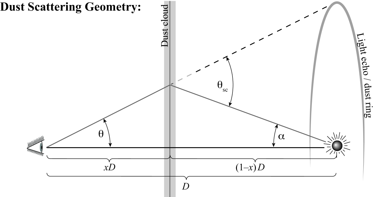
If the source exhibits a temporally well-defined flare followed by a period of quiescence, the scattering signal takes the form of discrete rings. The geometry of dust scattering echoes is described in detail by, e.g., Vianello et al. (2007); Tiengo et al. (2010); Heinz et al. (2015). Here, we will briefly summarize the basic geometric features of light-echo rings and define quantities used throughout the paper. The cartoon shown in Fig. 1 shows a simple sketch of the geometry.

For an X-ray source at distance $D$, X-rays traveling toward the observer can be scattered by intervening dust. A dust cloud at distance $D_{\rm dust}=xD$ (where $x$ is the fractional dust distance relative to the source distance) can scatter X-rays traveling along some initial angle $\alpha$ relative to the line of sight toward the observer, such that they arrive at an observed angle $\theta$ relative to the line of sight. The scattering angle is thus $\theta_{\rm sc}=\alpha+\theta$.

Because the scattered X-rays (observed at time $t_{\rm obs}$) have to traverse a longer distance, they will arrive with a time delay $\Delta t=t_{\rm obs}-t_{\rm flare}$ relative to the un-scattered X-rays (observed at time $t_{\rm flare}$), given by

$$\Delta t=\frac{xD\theta^{2}}{2c\left(1-x\right)}$$ (1)

If the dust along the line of sight is concentrated into dense clouds (such that the cloud extent is small compared to $D$), and if the X-ray flare is comparable to or shorter than $\Delta t$, the light echo will take the form of well defined rings with angular distance from the optical axis toward the source of

$$\theta=\sqrt{\frac{2c\Delta t\left(1-x\right)}{xD}}$$ (2)

Figure 1.— Cartoon of dust scattering geometry. X-rays from a source at distance $D$ are scattered off a dust layer at distance $xD$. The observed angle of the scattered X-rays is $\theta$, while the true scattering angle is $\theta_{\rm sc}=\theta/(1-x)$.

The (unabsorbed) intensity of the light echo is given by (e.g. Mathis & Lee, 1991)

$$I_{\nu}=N_{\rm H}\frac{d\sigma_{\rm sc,\nu}}{d\Omega}\frac{F_{\nu}\left(t=t_{\rm obs}-\Delta t\right)}{\left(1-x\right)^{2}}$$ (3)

where $d\sigma_{\rm sc}/d\Omega$ is the differential dust scattering cross section (per hydrogen atom), $F_{\nu}(t)$ is the flux of the flare at time $t$, and $N_{\rm H}$ is the hydrogen column density of the cloud responsible for the echo. Photo-electric absorption will attenuate this intensity by a factor $\exp{[-\sigma_{\rm ph,\nu}N_{\rm H,tot}]}$, where $N_{\rm H,tot}$ is the total hydrogen column along the path of the echo and $\sigma_{\rm ph,\nu}$ is the total photo-electric absorption cross section at frequency $\nu$.

For a short flare (i.e., flare duration $\delta t_{\rm flare}\ll\Delta t$ such that the ring is narrow and $d\sigma/d\Omega$ can be approximated as constant across the ring), the flux density from each ring (produced by the entire echo of a single cloud) at a given energy can be derived by integrating eq. (3) over $\theta$, holding $d\sigma/d\Omega$ constant:

$$F_{\rm ring,\nu}=\frac{2\pi cN_{\rm H}}{x(1-x)D}\frac{d\sigma_{\rm sc,\nu}}{d\Omega}{\mathcal{F}}_{\nu}$$ (4)

where ${\mathcal{F}}\equiv\int dtF$ is the fluence of the flare and $N_{\rm H}$ is the column density averaged over the entire ring. Equation (4) can be written for ring sections by integrating $I$ over a range in azimuthal angle $\phi\leq 2\pi$ to account for the fact that $N_{\rm H}$ can vary across the cloud, as discussed further in §4.2.

The scattering cross section depends strongly on scattering angle, with

$$\frac{d\sigma(\theta_{\rm sc},E)}{d\Omega} = \int_{a_{\rm min}}^{a_{\rm max}}da\,\frac{dN}{da}\frac{d\sigma(\theta_{\rm sc},E,a)}{d\Omega}$$ (5)

$$\sim \frac{d\sigma}{d\Omega}_{1000,1keV}\left(\frac{\theta_{\rm sc}}{1000^{\prime\prime}}\right)^{-\alpha}\left(\frac{E}{1keV}\right)^{-\beta}$$

with $\alpha\sim 3-4$ and $\beta\sim 3-4$ (e.g. Draine, 2003). Since the scattering angle is simply related to $\Delta t$, $x$, and $\theta$ by

$$\theta_{\rm sc}=\frac{\theta}{1-x}=\sqrt{\frac{2c\Delta t}{xD\left(1-x\right)}}$$ (6)

the intensity and the flux of the light echo decrease roughly as

$$F_{\rm ring}\propto\Delta t^{-\alpha/2}$$ (7)

with time delay $\Delta t$ between the flare and the time of the observation.

Observing X-ray light echoes can be used to study properties of the source as well as the intervening dust. For example, if the distance to the source is not known, one may use light echoes in combination with kinematic information from molecular gas to constrain the source distance (Predehl et al., 2000; Heinz et al., 2015).

On the other hand, if the source distance is known, the echo becomes a powerful probe of the distribution of interstellar dust, because eq. (2) can be solved for the dust distance $x$:

$$x=\frac{1}{1+\frac{D\theta^{2}}{2c\Delta t}}$$ (8)

thus allowing 3D maps of the interstellar dust toward the source to be constructed.

One may also constrain the properties of the X-ray dust scattering cross section (Tiengo et al., 2010). With good temporal coverage of the light echo, one can determine the dependence of the cross section on scattering angle (and thus constrain grain size distributions and scattering physics), and, with an accurate light curve of the outburst and an independent measure of the hydrogen column density toward the source, one may determine the absolute value of the scattering cross section per hydrogen atom.

Because the echo also contains information about the light curve of the outburst, it may conversely be used to set contraints on the fluence and temporal evolution of the outburst.

1.2. The July 2015 V404 Cyg Light Echo

V404 Cyg is a classical X-ray transient, hosting a $9^{+0.2}_{-0.6}\,M_{\odot}$ black hole in orbit with a K3 III companion (Khargharia et al., 2010). The distance of $D_{\rm V404}=2.39\pm 0.14\,{\rm kpc}$ to the source is known from VLBI parallax (Miller-Jones et al., 2009) with high precision.

Figure 2.— Lightcurve constraints; from bottom to top:bottom panel: INTEGRAL JEMX 3-7 keV lightcurve of the June 2015 outburst in crab units plotted against MJD. Broken gray bar at top shows coverage, with gray areas showing gaps in coverage; second panel from bottom: INTEGRAL SPI 20-100 keV lightcurve and coverage fraction (gray bars) of the June 2015 outburst in crab units plotted against MJD; third panel from bottom: Swift BAT 15-30 keV lightcurve of the outburst, same convention as bottom panel; third panel from top: cross-correlations of Chandra ObsID 17701 vs. 17704 (black) and Swift ObsID 00031403071 vs. 00031403079 (gray) plotted against time showing the peak of the outburst occurred on MJD 57199.8; second panel from top: Reconstructed lightcurve of the outburst from analysis of rings [a] and [b] of Chandra ObsID17704 (light gray curve), and the lightcurve deconvolved with the Chandra PSF (filled dark gray curve); top panel: Cumulative fluence of the outburst from INTEGRAL (light gray dash-triple-dot), Swift BAT (dark gray dash-dot) and reconstructed from Chandra (black), indicating that about 70% of the fluence from the outburst was due to the flare on MJD 57199.8.

After 26 years in quiescence, V404 Cyg went into outburst in June 2015 (Barthelmy et al., 2015; Negoro et al., 2015; Ferrigno et al., 2015; Rodriguez et al., 2015; King et al., 2015), with peak fluxes in excess of 10 Crab at hard X-ray energies. Shortly after the end of the outburst, a bright light echo in the form of several rings was observed in Swift images of the system. The echo was discovered and first reported by Beardmore et al. (2015). Both Swift and Chandra followed the temporal evolution of the light echo. An analysis of the Swift data of the echo was presented by Vasilopoulos & Petropoulou (2016), see also Beardmore et al. (2016).

In this paper, we present a combined, in-depth analysis of the Chandra and Swift data of the echo, introducing a new spectral modeling code to fit dust scattering echoes using XSPEC. Throughout the paper, we will use a default peak time of the outburst (the time of the brightest peak that contains the largest portion of the outburst fluence and is responsible for most of the echo and the bright rings observed) of

$$t_{\rm flare}={\rm MJD}\,57199.79$$ (9)

and delay times of observations $\Delta t$ will be referenced to this time and to the delay time between $t_{\rm flare}$ and the time of the first Swift observation, ObsID 00031403071,

$$\Delta t_{\rm 0}=3.68\,{\rm d}$$ (10)

We will motivate this choice of $t_{\rm flare}$ in §3.4. Position angles are measured clockwise from North in FK5 equatorial coordinates. Unless otherwise specified, quoted uncertainties are 3-sigma confidence intervals.

The paper is organized as follows: in §2 we discuss the reduction and basic analysis of the observations used in the paper. Section 3 presents an analysis of the intensity profiles of the observations. In §4, we present a new spectral modeling code for dust scattering signals and describe the spectral fitting technique used to jointly analyze the entire dust echo. Section 5 discusses the results of the analysis and compares them with previous works. Section 6 presents conclusions and a summary of our results.

2. Data Reduction and Analysis

2.1. The Swift BAT and INTEGRAL JEMX X-ray Light Curves of the June 2015 outburst

A reliable analysis of the V404 Cyg light echo requires accurate knowledge of the light curve and fluence of the outburst that caused the echo. Because V404 Cyg was extremely time-variable, with very short, bright flares (Segreto et al., 2015; Kuulkers, 2015), such a light curve would require full-time monitoring of the object. No single instrument operating during the flare observed the source with sufficiently complete coverage (even if combined) to provide such a light curve.

In particular, MAXI, the all-sky monitor aboard the International Space Station and the only dedicated soft (2-4 keV) X-ray monitor operating at the time, only observed the source with an uncalibrated instrument (GSC3) and no reliable light curve of the outburst is available (Negoro et al., 2015).

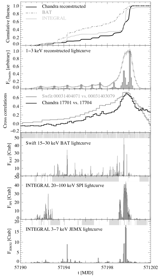
The Burst-Alert-Telescope (BAT) aboard the Swift spacecraft provided frequent hard-X-ray observations of the source in June 2015. The BAT light curve of the flare (Segreto et al., 2015) is plotted in the third panel from the bottom of Fig. 2, showing the highly variable behavior of the source. Plotted in gray above the light curve are the gaps due to visibility constraints given the low-Earth orbit of the spacecraft, bad data, and the pointing prioritization of other transient objects, indicating that the 14% duty cycle of the BAT was relatively small, and that many of the very short bright flares were likely missed. In consequence, the BAT light curve is insufficient for modeling the echo.

INTEGRAL’s JEMX instruments performed dedicated monitoring of V404 Cyg during June 2015 (Rodriguez et al., 2015; Ferrigno et al., 2015; Kuulkers, 2015). The segment-averaged 3-7 keV light curve is plotted in the bottom panel of Fig. 2, showing three bright flares as well as ongoing lower level activity through the period from MJD 57192 to 57200. The lightcurve was generated using standard pipeline processing of all INTEGRAL data taken during the outburst using the OSA software version 10.2.

The coverage by the telescope is continuous for most of the 72 hour orbital period of the spacecraft, however, the temporal coverage (again plotted as gray and white bars above the light curve) shows significant gaps during near-Earth passage, many overlapping with the gaps in BAT coverage, with a duty cycle of 40%, giving an approximate combined duty cycle of 48% of both telescopes.

INTEGRAL’s hard X-ray SPI telescope also observed the source during the flare (Rodriguez et al., 2015; Kuulkers, 2015); the 20-100 keV lightcurve is shown in panel 2 of Fig. 2, displaying the main flare as well as what appears to be a hard pre-cursor not visible in the JEMX lightcurve. The SPI lightcurve does not cover most of the time prior to the main flare.

Consequently, a full reconstruction of the hard X-ray lightcurve is not possible from the available coverage. Furthermore, the analysis of the echo requires knowledge of the soft X-ray lightcurve (1-3 keV). No instrument observed the source continuously in that band. However, as we will show in §3.4, it is possible to reconstruct the soft X-ray lightcurve of the outburst (with relatively low temporal resolution) from the Chandra images of the inner rings of the echo.

2.2. Chandra

Chandra observed V404 Cyg on 07-11-2015 for 39.5 ksec (ObsID 17701) and on 07-25-2015 for 28.4 ksec (ObsID 17704), as listed in Table 1. ObsID 17701 was taken with the High Energy Transmission Grating (HETG) in place, using ACIS CCDs 5,6,7,8, and 9, while ObsID 17704 was performed in full-frame mode without gratings, using ACIS CCDs 2,3,5,6,7, and 8. Because of the potential threat of lasting chip damage a re-flaring of the point source would have posed to ACIS, the point source in ObsID 17704 was placed in the chip gap between ACIS S and ACIS I using a SIM Offset of 17.55mm, and Y- and Z-Offsets of 1’.0 and -0’.3, respectively.

We reduced the data using CIAO and CALDB version 4.7. Because of the very small number of point sources visible in the field of view, we relied on the Chandra aspect solution of the observations to align the images. The accuracy of the aspect solution is typically much better than one arcsecond and sufficient for the purposes of this analysis.

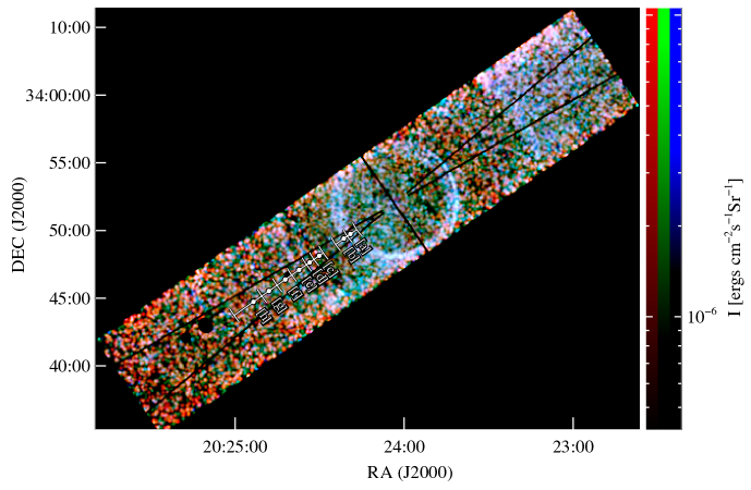
ObsID 17704 was background subtracted using the standard blank sky fields as described in the CIAO thread and Hickox & Markevitch (2006), matching hard counts above 10 keV in each CCD separately with the corresponding blank sky background files to calculate the effective exposure correction of the background. A three color image in the bands 0.5-1, 1-2, and 2-3 keV, smoothed with a 10”.5 Gaussian, is shown in Fig. 3. The image was extracted in equatorial (J2000) coordinates and also shows a compass with the axes of Galactic coordinates for orientation (Galactic North is at a position angle of about 55^∘).

Figure 3.— Three-color exposure-corrected image of Chandra obsID 17704 in the 0.5-1,1-2, and 2-3 keV bands (red, green, and blue, respectively), smoothed with a 10”.5 FWHM Gaussian. Arrow heads denote the brightest arclets of the inner two rings [a] and [b]. Overlaid are marks and labels denoting the location and spatial extent of spectral extraction regions of the eight rings identified in this paper.

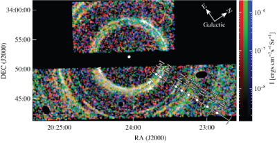
Background point sources in all images were identified using the wavdetect code in the CIAO package (Freeman et al., 2002) and removed before further processing. The image shows six clearly resolved, distinct rings of dust scattering emission which we label [a], [b], [c], [d], [e], and [g] from inside out in the analysis below (see corresponding labels in Fig. 4).

Because no blank background files exist for HETG data, and because the presence of the HETG significantly affects the background rates, we were not able to derive accurate backgrounds for ObsID 17701. Neither stowed nor blank background files produce residual-free background-subtracted images, which we attribute to the fact that soft protons focused by the mirrors are affected by the presence of the gratings, implying that neither blank nor stowed files are appropriate to use for HETG observations. Figure 5 shows a three color image of ObsID 17701 without background subtraction. Only the innermost rings of the echo, rings [a] and [b] in our notation below, are sufficiently above the background in ObsID 17701 to discern them by eye in the image.

The rings in the Chandra images are very sharp. For further analysis, we constructed radial intensity profiles for both ObsID 17701 and 17704 following the procedure outlined in Heinz et al. (2015), using 1000 logarithmically spaced radial bins between 3 and 20 arcminutes from the location of V404 Cyg.

The point-source position for ObsID 17701 is coincident with the known position of V404 Cyg. As mentioned above, for instrument safety reasons, the point source was placed in the chip gap between ACIS S and ACIS I in ObsID 17704. Using the profiles in five different 15 degree segments in the North-West quadrant of the inner rings [a] and [b] (all located on ACIS CCD 6), we verified that the centroid of the rings is coincident with the known position of V404 Cyg to within about an arcsecond, indicating that the Chandra aspect solution is accurate. No further reprojection of the aspect for ObsID 17704 was therefore needed.

2.3. Swift

For this work, we analyzed 50 separate Swift XRT imaging data sets of the light echo taken in photon-counting mode, as listed in Table 1. We further used 33 pre-flare data sets (ObsID 00031403002 to ObsID 00031403034), which we merged to construct a single clean sky background events file for subtraction in spectral analysis (not listed in Table 1). The table lists the fiducial time delay between the mean observation time and $t_{\rm flare}$. Data were pipeline processed using the standard Swift package in the HEASOFT distribution, version 6.17.

All pre-burst data were taken in 2012 during a previous monitoring campaign when the source was at a low flux. We stacked all pre-burst observations for a total exposure time of 138,716 seconds and searched for point sources. All identified point sources were excluded from spectral analysis.

Analysis of the pre- and post-outburst sets of the Swift observations indicates that attitude reconstruction of all event data incorrectly places the point source at the position (RA=20:24:03.970,DEC=+33:51:55.33), compared to the known source location of (RA=20:24:03.83,DEC=+33:52:02.2), offset by 7”, significantly more than the typical 3” single-observation pointing uncertainty. This suggests that the star tracker information used in attitude reconstruction may contain inaccurate stellar identifications. All Swift data were subsequently processed using a corrected source centroid determined from the emission-weighted position of the source from all 2012 observations. It is worth noting that the Swift point-source catalog (Evans et al., 2014) contains a source at the off-set position identified as 1SXPS J202404.2+335155 (derived from the 2012 observations) that is identical with V404 Cyg (identified properly in other catalogs).

Images and exposure maps were generated using standard ftools reduction tools. Background subtraction of spectra was performed using the sky background generated from the 2012 data.

Given its low-Earth orbit, the Swift particle background is both low and approximately constant with time. We verified that the diffuse hard (5-10 keV) background levels in both the 2012 and 2015 data are consistent with each other to better than 5% both in spectral shape and spatial distribution, within the typical Poisson uncertainties of the individual 2015 observations.

The soft 0.5-5 keV background (relevant for the analysis of the soft dust scattering echo) is dominated by astronomical sources, thus, background removal from the stacked sky file is appropriate even if the non-astronomical (particle) backgrounds would have changed moderately between 2012 and 2015.

To allow a single high-resolution image of the echo to be constructed, and for comparison with the Chandra data, we implemented a new echo stacking procedure. Figure 4 shows a stacked color image of all Swift exposures in the bands [0.5-1.0,1.0-2.0,2.0-3.0] keV. This image was constructed as follows: Each background-subtracted counts image and each exposure map was re-scaled in angular size by a factor $\delta_{\theta}\equiv\sqrt{\Delta t_{\rm 0}/\Delta t_{\rm obs}}$, centered on the position of V404 Cyg, to match the angular size of the echo in Swift ObsID 00031403071 (using equation 2), thus matching the peak position of each ring. That is, a photon at a given angle $\theta$ is re-mapped to a smaller angle $\theta_{0}=\theta\delta_{\theta}$ to match ObsID 00031403071.

Figure 4.— Three-color stacked exposure corrected Swift XRT image of the 2015 V404 Cyg light echo in the 0.5-1,1-2, and 2-3 keV bands (red, green, and blue, respectively). All 50 Swift observations listed in Table 1 were combined by scaling each image to the angular scale of the echo during the first observation, ObsID 00031403071 (using eq. 2) and corrected for temporal attenuation by a factor of $(1-x)^{2}(d\sigma/d\Omega)$ (cross section calculated according to the best fit in §5.1).

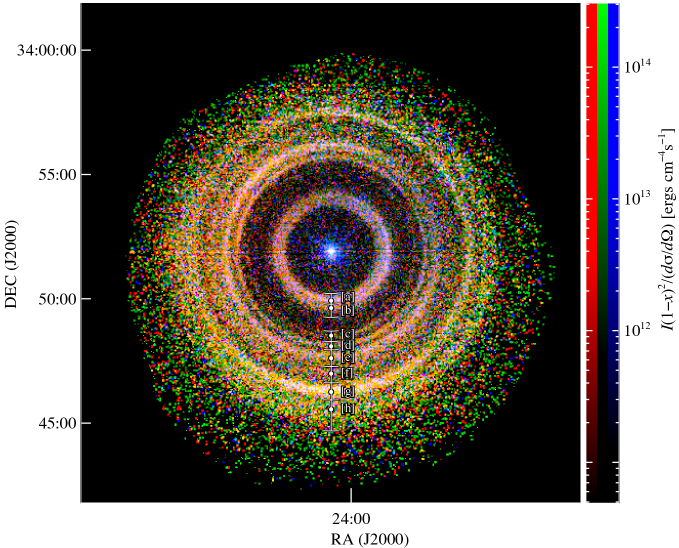
In the construction of this image, we implicitly approximated the lightcurve of the outburst as a single peak (see §3.4 for further discussion) to calculate the fractional dust distance $x$ and scattering angle $\theta_{\rm sc}$ for every pixel of the image, using eqs. (8) and (6), respectively. Each pixel in each of the counts images was then multiplied by the normalization factor $(1-x)^{2}/[d\sigma(\theta_{\rm sc})/d\Omega]$, using our best-fit MRN1 dust model to calculate $d\sigma/d\Omega$ (see §4.1 for details). The image brightness is thus proportional to $e^{-\tau_{N_{\rm H}}}N_{\rm H}{\mathcal{F}}$ (i.e., no correction for photo-electric absorption was made in the image). All scaled counts images were then stacked and divided by the stacked exposure map. The outer regions of the image become noise dominated since the total exposure used for those regions is significantly shorter than the central region.

3. Image analysis

The stacked image in Fig. 4 clearly shows the four bright rings identified in the discovery ATel (Beardmore et al., 2015) and the five rings identified in Vasilopoulos & Petropoulou (2016). In addition to the previously identified rings, the Chandra and the stacked Swift images show a number of fainter rings. In total, we identify eight separate rings in the Swift image (which has more complete spatial coverage than the Chandra image), labeled [a]-[h] from inside out, indicated in location and radial extent by white dots and characteristic inner and outer ring-radii, respectively, in Fig. 4. Rings [c], [f], and [h] were not included in the analysis by (Vasilopoulos & Petropoulou, 2016) because they are not apparent in individual Swift pointings — detection from the Chandra image and the stacked Swift image, as well as from the radial intensity profiles discussed in 3.1, is straightforward, however. The five rings discussed in Vasilopoulos & Petropoulou (2016) correspond to the rings [a], [b], [d], [e], and [g].

While the outskirts of the image are noisy, the image shows clearly that the rings are not azimuthally uniform. As we will discuss below, rings [a] and [b] also have significant radial sub-structure in the Chandra images.

A color gradient is apparent in Fig. 4, with bluer regions toward the Galactic plane (in the direction of position angle $55^{\circ}$, as expected for a gradient in column density and thus photo-electric absorption, toward the plane. We will discuss the asymmetry of the column density distribution in the field of view (FOV) relative to the position of V404 Cyg and its implications for image- and spectral analysis in §3.3.

Figure 5.— Three-color exposure-corrected image of Chandra obsID 17701 in the 0.5-1,1-2, and 2-3 keV bands (red, green, and blue, respectively), smoothed with a 10”.5 FWHM Gaussian.

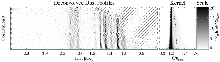
3.1. Radial Intensity Profiles and Time of the Peak Flare

Because the rings are concentric about the position of V404 Cyg, it is appropriate to construct radial intensity profiles. Following the analysis of the Circinus X-1 light echo in Heinz et al. (2015), we generated azimuthally averaged radial surface-brightness profiles for each observation centered on the (attitude-corrected) position of V404 Cyg. Profiles are computed on a logarithmic radial grid to allow for deconvolution with the annular profile of the light echo generated by a single thin dust sheet, which can be calculated from the soft X-ray lightcurve of the outburst (see Heinz et al., 2015, for details).

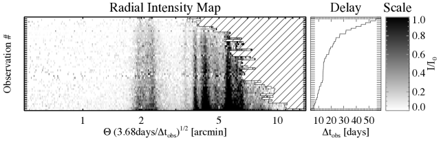
All 1-2 keV Swift profiles are shown in the left panel of Fig. 6 as a function of observation number and angular distance from V404 Cyg. Because the angular scale of the echo increases with time as $\theta\propto\Delta t^{1/2}$ according to eq. 2, the radial bins for the intensity profiles were chosen to increase by the same ratio, that is, the profiles were extracted in 300 logarithmically spaced bins between $\theta_{\rm min}=0^{\prime}.5\,\sqrt{\Delta t/\Delta t_{0}}$ and $\theta_{\rm max}=14^{\prime}\,\sqrt{\Delta t/\Delta t_{0}}$ such that the echo of the main flare on MJD57199.8 appears stationary on the grid of intensity profiles, displayed against the angular scale $\theta_{0}$ of ObsID 00031403071. The success of this method in capturing the main features of the echo can be seen from the vertical alignment of the echo from each ring in Fig. 6.

Chandra angular profiles were extracted on a finer angular grid than the Swift data to take advantage of the better angular resolution (and thus not over-plotted in Fig. 6).

Using eq. (3), the intensity scale of each row in the image was adjusted by a factor of $(1-x)^{2}\left(\theta_{\rm sc}/1000^{\prime\prime}\right)^{\alpha}$ [where we use $\alpha\sim 3$ from §5.1 and where the scattering angle is calculated using eq. (6), assuming the emission is dominated by the echo from the bright flare on MJD 57199.8] to remove (to lowest order) the strong temporal decline in echo brightness due to the increase in scattering angle, allowing us to show all profiles in a single image.

We analyzed the data in four energy bands, 0.5-1, 1-2, 2-3, and 3-5 keV. Profiles were background subtracted by constructing a clean sky and instrumental background level for the V404 Cyg field of view from the pre-flare XRT imaging observations.

Figure 6.— From left to right: (1) Map of the radial intensity profiles $I_{1-2}\left(1-x\right)^{2}\left(\Theta_{\rm sc}/1000^{\prime\prime}\right)^{\alpha}$ of all Swift images used in this analysis in the 1-2 keV band (with $\alpha=3.0$ from §5.1), as a function of observation number and angular distance $\Theta\left(\Delta t_{obs1}/\Delta t\right)^{1/2}$ from V404 Cyg  (the scaling factors remove the time dependence of the angular and intensity scale to lowest order). The hatched area shows the edge of the field of view. Vertical features correspond to individual clouds. (2) Delay time between main flare and Swift observation as a function of observation number. (3) Linear intensity scale used in the leftmost panel.

In order to explore the possibility of multiple flares undetected due to gaps in coverage, and in order to determine the time of the main flare, we plotted the cross-correlation of the radial profiles of the two Chandra data sets in the third panel from the top of Fig. 2 against the time of the flare (calculated from the time lag). The cross-correlation shows a clear peak on MJD 57199.8, indicating that the main flare that gave rise to the rings does indeed correspond to the main flare seen by INTEGRAL, consistent with the findings in Vasilopoulos & Petropoulou (2016). The figure also shows the cross-correlation of the intensity profiles of Swift ObsID 0031403071 and 0031403079, which shows the most well-defined peak of all the Swift cross-correlations (all other cross-correlations of Swift profiles are less well defined). The peak is consistent with the peak derived from the Chandra data, though with somewhat broader wings.

3.2. The Width of Rings [a]-[d]

The innermost two rings [a] and [b] overlap significantly in the Swift image, but are clearly resolved in both of the Chanda images. It is also clear that the rings are not azimuthally symmetric, both in color and total intensity in all images, which will be discussed further in §3.3.

Figure 3 shows that several of the rings are very sharp. In particular, the two innermost rings [a] and [b] contain bright, sharp arclets in the Southern and North-Western halfs of the rings, respectively, denoted by arrow-marks in the figure. Rings [c] and [d] also appear sharp, while the outer rings [e] and [f] appear broader in Fig. 3. We identify the sharp brightness peaks with the echo from the main flare at the end of the outburst on MJD 57199.8. Emission from earlier sub-flares of the outburst will be located at larger angles according to eq. (2).

Figure 7.— Radial intensity profiles across rings [a]-[d] (taken at position angles $90^{\circ}-270^{\circ}$, $9.5^{\circ}-72^{\circ}$, $90^{\circ}-270^{\circ}$, and $90^{\circ}-270^{\circ}$, respectively) in the 1-2 keV band from Chandra obsID 17704 (black histograms). Overplotted are Gaussian fits to the ring components (black curves) and radial profiles of the 1-2 keV Chandra PSF at the location of rings (filled gray histograms). For comparison, the red histogram in panel [b] shows the radial profile for ring [b] taken at position angles $167^{\circ}-333^{\circ}$.

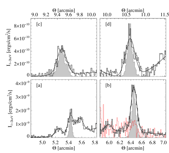
Figure 7 shows the radial 1-2 keV intensity profile across the brightest segments of rings [a]-[d] in Chandra ObsID 17704. Ring [a] was extracted between position angles $90^{\circ}-270^{\circ}$, ring [b] over position angles $9.5^{\circ}$ and $72^{\circ}$, and rings [c] and [d] over the entire region covered by the chips of the ACIS S array, roughly from position angle $90^{\circ}$ to $270^{\circ}$.

Because of the large angular size of the rings (5’.5, 6’.44, 9’.5, and 10’.6, respectively), the Chandra point-spread-function (PSF) is significantly wider than near the aim point, and a by-eye inspection of the width of the rings is insufficient to determine whether the rings are resolved or not.

In order to evaluate whether the rings are resolved, we generated matched Chandra PSFs using CHART/MARX at the positions of the peak intensities of the rings, using the aspect file for ObsID 17704. The simulated PSFs were reduced identically to ObsID 17704; radial surface-brightness profiles of the PSFs at the radii of rings [a]-[d] are over-plotted in gray in Fig. 7 on the narrowest and highest peak of the respective ring. All rings are marginally resolved. Ring [a] shows clear sub-structure with at least three sub-peaks, of which we chose the narrowest for comparison.

From equation 2, the radial extent of each ring is determined by both the line-of-sight extent $\Delta x$ of the cloud responsible for the ring and the structure of the light curve (i.e., the temporal width of the flare responsible for the ring).

The sharpness of the rings implies very concentrated dust clouds responsible for the rings and a very sharp peak in the flare lightcurve. Given the gaps in the lightcurve coverage, we cannot distinguish whether the width is due to spatial cloud extent or duration of the flare. However, we can place upper limits on the FWHM line-of-sight extent of the four clouds [a]-[d]. These are listed in Table 2, along with the inferred distances to the clouds.

In particular, we find an upper limit on the line-of-sight extent of cloud [b] of $D_{\rm[b]}\mathrel{\hbox{\hbox to0.0pt{\hbox{\lower 4.0pt\hbox{$\sim$}}\hss}\hbox{$<$}}}8.8\,{\rm pc}$. This is comparable to the transverse size scale of $L_{\rm[b]}\sim 5\,{\rm pc}$ for cloud [b] inferred from the angular size of the brightest ringlet, which is roughly 7 arcminutes across, and, since the clouds responsible for rings [a]-[h] have roughly comparable column density, the extent along the line of sight is comparable to the expected typical cloud size toward V404 Cyg in general.

3.3. The Non Axi-Symmetry of Rings [a] and [b]

As was found in Heinz et al. (2015), rings from dust scattering echoes can show significant deviations from axi-symmetry due to variations in the column density of the scattering dust concentrations. Asymmetries have also been found in a number of dust scattering halos by Seward & Smith (2013), Valencic & Smith (2015) and McCollough et al. (2013).

For typical physical clump sizes of order a few parsec, appropriate for moderate-mass clouds with hydrogen column densities of order $10^{21}\,{\rm cm^{-2}}$ (e.g. Larson, 1981; Heyer et al., 2009), the typical angular scale of clouds between us and V404 Cyg will be of the order of a few arcminutes to tens of arcminutes and thus potentially smaller than the FOV covered by the echo. For random placement of clouds, we should therefore expect that the different clouds responsible for the rings (a) will not be centered on the position of V404 Cyg, and (b) may show significant density gradients across the FOV. Furthermore, since the source is about 2 degrees south of the Galactic plane, we would expect cloud centroids to be preferentially off-set to the North-West of V404 Cyg, in the direction toward the Galactic plane.

This should induce a deviation from axi-symmetry in the brightness distributions of the rings, and it should also lead to non-monotonic radial brightness evolution as the rings expand, complicating analysis of the dust scattering signal, because the column density of each cloud cannot necessarily be considered uniform across the image.

Of all rings visible in Figs. 3 and 4, ring [b] shows the clearest signs of deviation from axi-symmetry, with the North-West section of the ring being much brighter than the other three sections. The spectrum of the North-West section of ring [b] is also much harder, supporting the notion that cloud [b] has a much higher column density in the North-West direction, which increases both the scattering intensity and the amount of photo-electric absorption.

Because the photons for each scattering ring must pass through all clouds along the line of sight (either before or after scattering), the azimuthal variation in the column in each cloud will be imprinted on all scattering rings. Thus, some of the general trend of the color in Fig. 4 can be attributed to cloud [b] alone. The compounded azimuthal asymmetry of the absorption column must be included when modeling the emission of the rings and will be described in more detail in §4.2.

The bottom-right panel of Fig. 7 shows a comparison of the 1-2 keV angular profiles of ring [b] from the North-West quadrant (black curve) to the Eastern half of the ring (red curve), indicating that the North-Western part is about four times brighter than the Eastern part of the ring.

We quantified this by simple parametric spectral fits to the four quadrants of rings [a] and [b] of Chandra ObsID 17704. We extracted spectra of the rings in annular sections in the North-West, South-West, South-East, and North-East quadrants and fit them with a simple absorbed powerlaw model (${\tt phab}\cdot{\tt powerlaw}$ in XSPEC), where the powerlaw model, written in photon flux $\phi_{E}$, takes the form

$$\phi_{E}=\phi_{0}\left(\frac{E}{1\rm keV}\right)^{-\Gamma}$$ (11)

We tied the powerlaw slope of all spectra across all rings but left the photo-electric column $N_{\rm H}$ and the powerlaw normalization for each ring as free parameters. The resulting fit parameters and uncertainties are listed in Table 3.

We find that, for ring [b], the normalization of the powerlaw (i.e., the scattered intensity after removing the effects of photo-electric absorption) is a factor of 4 larger than in the other three quadrants, a highly significant deviation, while ring [a] is brightest in the South-Western quadrant. The photo-electric neutral Hydrogen column density in the North-West quadrant for both rings [a] and [b] is larger by about $3\times\,10^{21}\,cm^{-2}$ than in the other three quadrants. Since ring [a] is not brighter in this direction, we attribute the increase in column density primarily to ring [b], though it must be kept in mind that the total photo-electric column is expected to increase toward the Galactic plane in the North-West direction, and therefore the total column of clouds [c]-[h] will likely, on average, be larger in the North-West quadrant.

This is clear evidence that the centroid of cloud [b] is off-set from the direction of V404 Cyg and that the dust scattering column density cannot be assumed uniform across the image. By extension, we cannot make the assumption of uniform column density for any of the clouds in our analysis of the dust scattering echo.

To test the azimuthal uniformity of the different clouds, we generated stacked cloud images of all Swift observations in the 1-2 keV band, where the signal-to-noise is highest. The result is shown in Fig. 8.

Figure 8.— Reconstructed cloud images in the 1-2 keV band, calculated from stacking all Swift images for each individual ring (using the radial bins indicated in Fig. 4 for each ring) and binning them into 32 azimuthal sections. The image is scaled by $x(1-x)D/({\mathcal{F}}\Delta\varphi\,c\,d\sigma/d\Omega)$ to show the absorbed column density $e^{-\tau}N_{\rm H}$ according to eq. (4), where ${\mathcal{F}}$ and $d\sigma/d\Omega$ are taken from the best fit spectral model discussed in §5.1 and $\Delta\varphi=11.25^{\circ}=0.196\,{\rm rad}$ is the angular bin size. The images show clear column density variations across the field for each cloud. Overlaid on panel [b] are contours of excess extinction $\Delta E(B-V)=0.4$ (dashed) and $\Delta E(B-V)=0.8$ (solid) in the 2-2.5 kpc distance range from Pan-STARRS, coincident with the peak in column density of cloud [b].

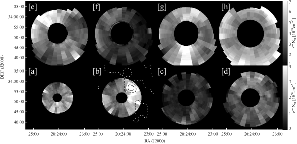
To generate the cloud images, we divided each XRT image into eight rings (denoted by the white marks in Fig. 4 in units of $\theta_{0}$, adjusted to the angular scale of the observation using eq. 2, that is, the ring extraction is performed in sky coordinates $\theta$, not in scaled coordinates $\theta_{0}$), and each ring into 32 azimuthal bins, and derived the 1-2 keV flux of each bin from the total exposure corrected count rate.

Following eq. (4), the flux in each bin was multiplied by a factor $x(1-x)D/[\Delta\varphi c{\mathcal{F}}(d\sigma/d\Omega)]$ to remove, to lowest order, the dependence on cross section and cloud distance $x$. Here, $\Delta\varphi=11.25^{\circ}=0.196\,{\rm rad}$ is the angular size of each bin. We used best-fit values for the cross section and fluence from our fiducial MRN1 spectral model listed in §5.1. Each bin therefore contains a local measure of $e^{-\tau_{\rm ph}}N_{\rm H}$, i.e., not corrected for photo-electric absorption. Note again that each cloud affects all rings by photo-electric absorption at an angular scale set by the relative distances to the cloud responsible for the scattering and that responsible for the absorption. The compounded effect of photo-electric absorption is treated in detail in §4.2. All 50 images for a given ring were then stacked — at the actual physical angular scale $\theta$ rather than scaled to $theta_{0}$ — to produce a single dust map of the cloud generating the ring.

The outer regions of the images are noisy, but there is clear evidence of non-uniformity in all of the cloud images. In particular, cloud [b] appears to have a strong local peak in the North-West quadrant centered on location (RA=20:23:40.9,DEC=33:56:39).

We tested the significance of the azimuthal variations by summing all angular profiles in the 1-2 keV band used to construct Fig. 8 along the radial direction for each cloud, thus creating 1D azimuthal intensity profiles, shown in Fig. 9.

The azimuthal intensity peaks in rings [a], [b], [d], [e], [f], and [g] are clearly visible in Fig. 9. The measured variance in the profiles is larger than the mean error in the intensity by factors of 3.4, 5.6, 2.1, 5.0,10.1,5.4,5.3, and 2.6 from ring [a] to [h], respectively, indicating that the angular variations seen in the profiles are significant. Note that error bars indicate the 1-sigma Poisson uncertainties in each angular bin.

Figure 9.— Angular column-density profiles constructed by summing each radial bin in Fig. 8 in radius. Error bars indicate 1-sigma Poisson errors in each bin.

3.4. Reconstruction of the Soft X-ray Lightcurve of the Outburst from the Chandra Light Echo

In §3.5, we will employ the same radial-deconvolution technique of the ring profile used in Heinz et al. (2015) to recover the dust distribution along the line of sight. That is, we use the fact that for a thin scattering sheet of dust the intensity profile of the light echo is described by eq. (3) for a single $x$ and use eq. 2 to relate $\Delta t$ to $\theta$.

If the complete light curve $F(\Delta t)$ of the outburst is known, and we make the assumption that the scattering cross section can be reasonably approximated as a powerlaw in scattering angle $d\sigma/d\Omega\propto\theta_{\rm sc}^{-\alpha}$ over a moderate range in scattering angle, the radial intensity profile can then be decomposed into dust echoes from a series of scattering screens along the line of sight, using the kernel function

$$K(z)=F(\Delta t_{\rm flare}z^{2})z^{-\alpha}$$ (12)

where $z\equiv\theta/\theta_{\rm flare}$ and $\theta_{\rm flare}=\theta(\Delta t_{\rm flare})$ from eq. (2), using $\Delta t_{\rm flare}\equiv t_{\rm obs}-t_{\rm flare}$. Such a deconvolution will yield a distribution of scattering depth as a function of fractional dust distance $x$:

$$\Delta\tau(x)=\frac{\Delta N_{\rm H}}{\left(1-x\right)^{2}}\frac{d\sigma}{d\Omega}$$ (13)

The deconvolution is computationally straight forward if the radial profiles are extracted on logarithmic bins. We employ the Lucy-Richardson maximum-likelihood deconvolution (Richardson, 1972; Lucy, 1974) implemented in the IDL ASTROLIB library.

In the case of the V404 Cyg outburst, the gaps in coverage of the light curve (and the fact that no soft-X-ray telescope observed the outburst frequently enough to provide a reliable 1-2 keV light curve) do not allow the direct application of this technique. However, we can use the high angular resolution of Chandra and the non-axisymmetric brightness profile of ring [b] to reconstruct the light curve of the V404 Cyg outburst. We will then use this reconstructed light curve in our deconvolution of the echo.

From the profile shown in Fig. 7b and the spectral extraction discussed in §3.3, we know that the column density toward cloud [b] is much larger in the North-West quadrant than in any other quadrant, while cloud [a] and any intervening clouds between cloud [a] and [b] (which may contribute to ring emission in the annular range between 5’ and 7’), are not strongly concentrated in the North-West quadrant.

We also know from the image and analysis of the intensity profiles that the annuli outside of ring [b] between 7’ and 9’.2 do not show evidence of ring emission. Thus, the emission in the North-West quadrant from about 6’.2 outward is dominated by emission from ring [b]. We can therefore use the difference in intensity between the North-West quadrants and the Eastern quadrants to isolate emission from cloud [b] only.

To lowest order, this difference will be the emission produced by the excess in column density of cloud [b] in the North-Western quadrant and will correspond the the light echo of a single, thin cloud of dust. The bright peak of ring [b]_NW is clearly due to the main flare of the outburst. We expect lower intensity emission from prior sub-flares of the outburst to lie in the angular range from 6’.5-7’.4.

In order to extract this scattering response, we employed an iterative difference procedure between the Eastern and North-Western intensity profiles, isolating the difference in profiles from 6’.3 outward to construct the dust scattering kernel (that is, the intensity profile produced by cloud [b] only).

We first constructed a zero-order kernel by deconvolving the North-West profile of ring [b] with the Chandra PSF for ring [b] discussed in §3.2 and selected only emission outward of 6’.3 (that is, we reject any difference in the intensity profiles inward of the brightest peak in the intensity profile of ring [b], which we attribute to the flare at the end of the outburst, such that any additional emission from ring [b] must lie at larger angles). We re-convolved this profile with the Chandra PSF to derive the zero-order kernel function $K(z)_{0}$, using $\alpha\sim 3.0$ for our best-fit standard MRN1 dust scattering cross section from §5.1.

We then deconvolved the Eastern intensity profile in the angular range 5’.0-7’.4 with $K(z)_{0}$, isolated the deconvolution to contributions outward of 6’.3 (setting the interior to zero), re-convolved with $K(z)_{0}$ and subtracted the result from $K(z)_{0}$ to derive the next iteration in the kernel, $K(z)_{1}$. We repeated the procedure until the total absolute fractional difference between two iterative kernel functions $K(z)_{n}$ and $K(z)_{n+1}$ was less than $10^{-4}$ (convergence was reached after 5 iterations).

This procedure self-consistently accounts for the emission both from ring [b] as well as contamination from dust responsible for emission interior to ring [b] (which will contribute to the total intensity outward of ring [b] given the length of the outburst).

From this self-consistently derived kernel, we can reconstruct the X-ray light curve by inverting eq. (12). The resulting light curve is plotted in the second top-most panel in Fig. 2, both in its deconvolved form and convolved with the Chandra PSF. We used the latter for analysis.

The statistical uncertainties plotted in the figure were calculated using Monte-Carlo simulations by randomizing the intensity profiles with the appropriate amount of Poisson noise and repeating the iterative deconvolution procedure for each of the 1000 realizations.

The re-constructed light curve shows a clear peak at MJD 57199.8, within 0.2 days of the main flare of the outburst identified by INTEGRAL (bottom two panels) and the cross-correlations (third panel from the top). The deconvolution suggests that the flare may have had two peaks, but following the discussion in §3.2, we cannot distinguish whether the width of ring [b] is due to the properties of the flare or the line-of-sight distribution of cloud [b]. The smooth curve indicates that the temporal resolution of our iterative reconstruction is about a half day, and any claims for a double-peaked lightcurve on timescales shorter than that would be speculative at best.

The reconstructed light curve shows a broad tail of emission between MJD 57192 and 57199, consistent with the level of activity seen in the hard X-rays by both Swift BAT and INTEGRAL JEMX. The lack of any significant peaks in the tail suggests that no major flares were missed despite the gaps in coverage.

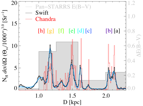
The cumulative fluence of the Chandra-reconstructed light curve (plotted in the top panel of Fig. 2) is consistent with the fluence distribution of the INTEGRAL lightcurve. Both suggest that about 70% of the total outburst fluence were concentrated in the major flare on MJD 57199.8. Using a single flare time and analyzing the echo based only on the major flare on MJD 57199.8 would thus miss about a third of the fluence in the roughly week-long precursor to the main flare. The emission-weighted mean precursor time is $t_{\rm pre}=$ MJD 57195.3.

3.5. The Dust Distribution Toward V404 Cyg

With a reconstructed outburst lightcurve in hand, we can employ the deconvolution procedure used in Heinz et al. (2015) and outlined in §3.4 to derive the dust distribution toward V404 Cyg. The kernel defined in eq. 12 used for this deconvolution is a function of time: For earlier observations, the range in angle spanned by the kernel is larger, that is, the rings from earlier observations are more spread out. This is visible in Fig. 6, which clearly shows the rings narrowing with time (relatively to their angular siez). For a total outburst duration of $\delta t_{\rm burst}\sim 9\,{\rm days}$, the angular spread at late observing times evolves roughly as

$$\frac{\Delta\theta}{\theta}\sim\sqrt{\frac{\delta t_{\rm burst}}{\Delta t_{\rm obs}}}.$$ (14)

This effect can be seen in the vertical “thinning” of the intensity profiles in the left panel of Fig. 6 and of the outer envelope of the kernel function plotted in the right panel of Fig. 10. The dashed contour in Fig. 10 shows the region of the kernel containing 80% of the kernel flux. Note that this contour does not exactly track the thinning described in eq. (14) because the part of the kernel at larger scattering angles become brighter with time relative to the part of the kernel at smaller angles as the range in scattering angles spanned by the kernel decreases.

Figure 10.— From left to right: (1) Map of deconvolved intensity profiles as a function of dust distance; (2) deconvolution kernel used to derive panel (a) from Fig. 6, calculated using eq. 12 and the reconstructed outburst lightcurve from Fig. 2. The dashed lines indicate the 10% and 90% flux contours, i.e., 80% of the kernel flux is contained in the area between the lines; (3) intensity scale bar for panel (1).

Each radial profile is deconvolved with the appropriate kernel. In order to correct for the dependence of intensity on $x$ and $\theta_{\rm sc}$ (see eq. 3), we multiply each deconvolution by $(1-x)^{2}\left(\theta_{\rm sc}/1000^{\prime\prime}\right)^{\alpha}$, where $x$ and $\theta_{\rm sc}$ for each angular bin are calculated from equations (8) and (2), respectively, and mapped to the corresponding distance $D=xD_{\rm V404}$, and we use $\alpha\sim 3.0$. The resulting curves measure the scattering depth $\Delta\tau_{\rm sc}=e^{-\tau_{\rm ph}}\Delta N_{\rm dust}\frac{d\sigma}{d\Omega}(1000^{\prime\prime})$ and are thus proportional to the dust column density, not corrected for photo-electric absorption. The resulting scattering depths of all Swift observations are plotted in the left panel of Fig. 10.

We will derive properly un-absorbed column densities of the different clouds in §5.1. However, all of the rings are affected by absorption in a similar fashion: the total column affecting each ring is just the sum of the column densities of all clouds. Moderate differences in the total absorption will arise from the azimuthal variations in each ring. The derived deconvolutions then allow us to derive the relative distribution of dust along the line of sight.

To derive a high signal-to-noise 1D dust distribution along the line-of-sight, we performed a weighted average of the dust distributions from each Swift observation, plotted as a black histogram in Fig. 11. Over-plotted in red is the dust distribution derived from Chandra ObsID 17704.

The histograms show at least eight separate clouds (as identified in Fig. 4), labeled [a]-[h], following the above naming convention, confirming the by-eye identifications in the stacked image in Fig. 4. The positions and scattering depths of the clouds derived from Swift and Chandra are consistent with each other out to the edge of the Chandra FOV (at distances larger than 1.2 kpc). Clouds [a] and [b] show higher column in the Chandra deconvolution, which we attribute to the fact that cloud centroids are clearly offset from the position of V404 Cyg (as discussed in §3.3): the Chandra observation was taken late during the echo, with rings [a] and [b] intersecting the cloud centroid, while the weighted average Swift dust distribution contains earlier, high signal-to-noise observations that are expected to have lower mean $N_{\rm H}$ for rings [a] and [b].

For further analysis, we fitted each of the eight clouds with a Gaussian, over-plotted in blue in Fig. 11. As expected from the higher angular resolution of the Chandra maps, the peaks in the dust distribution derived from ObsID 17704 are narrower. The Chandra profile (see Fig. 7) also suggests the presence of additional rings between [a] and [b], which are not discernible in the Swift profile. We label these rings as ring [a.2] and [b.1], while we label the main ring as rings [a.1] and [b.2]. In Table 4 we list the positions and line-of-sight widths inferred from the Gaussian fits. Where rings are sufficiently covered by Chandra, we list the Chandra values for their higher precision in distance and depth and split rings [a] and [b] into separate components, determined from Chandra ObsID 17704. The table also lists the mean and the variance of the cloud column densities, as well as parameters of the grain size distribution, determined from spectral fits described in §4 and §5.

For reference, we overplot the dust distribution from the $\Delta E(B-V)$ extinction map from Pan-STARRS in gray (Green et al., 2015). The $E(B-V)$ spatial resolution is insufficient to map each cloud to an individual extinction peak, but the general distribution is consistent, with rings [e]-[h] corresponding to the majority of the dust, and a clear peak at the positions of rings [a] and [b]. The low value of $E(B-V)<0.1$ short-ward of 1 kpc and the lack of any jumps in extinction in that distance range suggests that clouds [a]-[h] contain essentially all of the dust between us and V404 Cyg (see also the discussion in §5.1).

Clearly, the power of an extensive series of observations as provided by Swift lies in the ability to probe both the dust distribution and the dust scattering cross section over a large range in parameters. However, this also presents a key challenge to the analysis: Our discussion in §3.3 shows that we cannot assume that the dust column density is uniform across the FOV traversed by the echo. Because image analysis can only measure the scattering depth $\Delta\tau$, which depends on both the scattering cross section and the column density, it is impossible to derive both from an analysis of intensity profiles. In other words: simply by measuring a slope in the ring intensity as a function of ring- (and thus scattering-) angle, we cannot distinguish whether this slope is induced by a change in dust column density with angle or a slope in the scattering cross section as a function of scattering angle.

However, for a given cloud, we can expect the photo-electric absorption column to be proportional to the dust scattering column (e.g. Corrales & Paerels, 2015). We can then hope to spectrally disentangle the ambiguity between $N_{\rm dust}$ and $d\sigma/d\Omega$ by spectrally fitting the entire echo, and tying the scattering and absorption columns of each cloud together by a simple proportionality constant. This approach requires an accurate spectral model of the dust scattering cross section. We will discuss our spectral analysis of the Swift echo in the next section.

4. Spectral analysis of the echo

4.1. dscat: An XSPEC Model for Differential Dust Scattering Cross Sections

A spectral fit of the dust scattering echo using equation (3) or (4) requires a spectral model of the differential scattering cross section as a function of scattering angle and energy. No such model exists for the XSPEC package used for fitting the ring spectra in this paper.

We generated table models for $d\sigma/d\Omega$ for the most commonly used dust distributions and will briefly describe the computational method used to calculate the cross sections. Our dscat code for the differential scattering cross section is based on the public xscat package released by Smith et al. (2016) that presents xspec table models of integrated scattering cross sections; that paper contains a detailed description of the methodology used in calculating dust scattering cross sections.

Cross sections in this paper are calculated using exact Mie scattering solutions (rather than using interpolations or employing the common Rayleigh-Gans approximation, e.g., Mauche & Gorenstein, 1986), employing the publicly available Mie scattering code MIEV (Wiscombe, 1979, 1980). We include spherical harmonic expansions up to order 250 in MIEV to allow convergence at larger grain sizes.

Scattering cross sections depend on the imaginary part $k$ of the optical constant $m=n+ik$, which is related to the photo-electric absorption cross section $\sigma_{\rm ph}$ by the optical theorem

$$k=n_{\rm gr}\lambda\frac{\sigma_{\rm ph}}{4\pi}$$ (15)

where $n_{\rm gr}$ is the particle density of the dust grains and $\lambda$ is the X-ray wavelength of the photons under consideration.

The optical constants $n$ for different grain compositions used as input to the MIEV Mie-scattering code are taken from Zubko et al. (2004), which themselves are based on the photo-ionization cross sections provided by Verner et al. (1996), using the Kramers-Kronig relations to derive $n$.

We computed cross sections in the energy range $0.5\,{\rm keV}\leq E\leq 5\,{\rm keV}$ in 100 logarithmically spaced energy bins and over a range of scattering angles between $500^{\prime\prime}\leq\theta_{\rm sc}\leq 4500^{\prime\prime}$, in 100 logarithmically spaced angle bins. The computed model grids are written into FITS tables and cross sections at specific energies and scattering angles are calculated in XSPEC using logarithmic interpolation in angle and energy.

Following Smith et al. (2016), we implemented four families of dust distributions as functions of grain size $a$:

1. A generalized Mathis-Rumpl-Nordsieck (1977, MRN77 hereafter) distribution, which consists of a combination of silicate and graphite grains, each following a distribution with a single slope of

   $$\frac{dN_{\rm MRN}}{da}\propto a^{-\psi}$$ (16)

   with a default slope of $\psi_{\rm MRN}=3.5$, extending from $a_{\rm min}=0.005\mu{\rm m}$ to a maximum grain size of $a_{\rm max}$ with a default value of $a_{\rm max,MRN}=0.25\mu{\rm m}$. The default values correspond to the parameter choices of the orignal MRN77 model.

   We calculated cross sections over a range in slope $2.5\leq\psi\leq 5.5$ in 31 linearly spaced bins and over a range in maximum particle size $0.025\mu{\rm m}\leq a_{\rm max}\leq 8.5\mu{\rm m}$ in 39 logarithmically spaced bins; within this grid, dscat interpolates linearly and logarithmically in $\psi$ and $a$, respectively. Cross sections were calculated separately for silicate and graphite grains, adding both contributions together to calculate the differential cross section per hydrogen atom using solar abundances. In spectral fitting, we either fix $\psi$ and $a_{\rm max}$ across all clouds (thus imposing identical dust distributions on all clouds), which we call the MRN1 model, or we allow these parameters to vary from cloud to cloud (thus fitting eight different distributions), which we call the MRN8 model.

2. The 32 separate dust distributions derived and presented explicitly in Weingartner & Draine (2001, WD01), using the parameters and model names employed in Tables 1 and 3 of that paper. We refer to all of these as WD01 models with names based on the parameters of each model. These dust distributions were originally developed to describe a range of extinction measurement for Milky Way, LMC, and SMC sightlines and span a range in $R_{\rm V}$ values and composition.

3. The 15 separate dust distributions by Zubko et al. (2004, ZDA04), using the parameters and model names presented in that paper with a correction for the $b_{1}$ and $b_{2}$ parameters of the COMP models. These dust distributions were originally derived to fit Milky Way extinction and IR dust emission constraints and contain a range of grain compositions.

4. The dust distribution presented in Witt et al. (2001, WSD01), derived to describe the scattering properties of X-ray dust scattering halos, using a modified MRN77 distribution with a larger maximum grain size of $a_{\rm max,WSD}=2$ and steeper grain size distribution of $\psi_{\rm WSD}=4$ for grains larger than $0.4\mu{\rm m}$.

Each model contains as parameters the scattering angle, the dust column density, and the photon energy, while the generalized MRN models also allow $\psi$ and $a_{\rm max}$ to vary.

4.2. Spectral Modeling of the 2015 V404 Cyg Echo

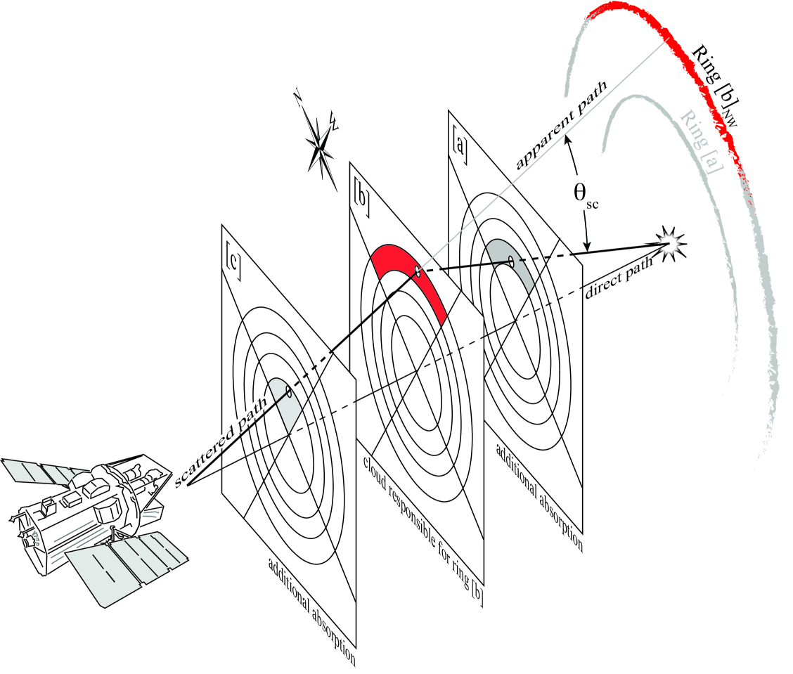
The scattering geometry of ring [b] (taken as an illustrative example) is sketched in Fig. 12. Because clouds cannot be assumed to be spatially uniform across the field of view, we divide each cloud into four annuli and each annulus into four quadrants (North-West, South-West, South-East, and North-East, measured in equatorial coordinates). As the light echo expands with time, each ring (i.e., the echo from each cloud) will sweep across the annuli. For the sake of computational feasibility, we will assume that the column density of a cloud is constant within each of the sixteen annulus sections.

It is clear from this figure and eq. (4) that the spectrum of (for example) ring $[b]$ in a given ring quadrant (spanning an azimuthal range of $\Delta\varphi=90^{\circ}=\pi/2)$, under the assumption of a short flare, is given by

$$F_{\nu}=e^{-\sigma_{\rm ph}(\nu)\sum_{i={\rm[a]}}^{\rm[h]}N_{\rm H,i}(\theta_{i})}\frac{\pi}{2}\frac{cN_{\rm H,[b]}}{x\left(1-x\right)D}\frac{d\sigma_{\rm sc}(\theta_{\rm sc},\nu)}{d\Omega}{\mathcal{F}}_{\nu}$$ (17)

where the photo-electric absorption term includes all the gas along the LOS (including cloud [b]). The same expression holds for all other clouds. We assume that most of the cold absorbing gas is located within the clouds responsible for the echo, but test for the presence of additional absorbing gas by allowing for an additional amount of (uniform) foreground absorption of gas and dust not located within clouds [a]-[h]. Scattering angles are calculated from eq. (6) using cloud positions from Table 4, assuming the time delay from Table 1.

We represent the flare spectrum by a simple powerlaw with normalization and powerlaw index as free parameters.

We incorporate photo-electric absorption using the PHABS table model in XSPEC for computational speed. The column density of each cloud that is used to calculate the total absorption column in eq. 17 will be a function of impact parameter and azimuthal angle (see §3.3). The impact parameter (in terms of angle on the sky) can be related to the observed ring angle by simple geometry using Fig. 12: for absorption by clouds closer to the observer than the scattering cloud (for illustrative purposes, clouds [c] and [b], respectively, in the cartoon in Fig. 12), the impact parameter is at the same on-sky off-axis angle, $\theta_{\rm[c]}=\theta_{\rm[b]}$. For absorbing clouds further away than the scattering cloud (cloud [a] and [b] in the cartoon in Fig. 12, respectively), the impact parameter is given by the on-sky off-axis angle $\theta_{\rm[a]}=\theta_{\rm[b]}[x_{\rm[b]}/(1-x_{\rm[b]})][(1-x_{\rm[a]})/x_{\rm[a]}]$.

Because, at a fixed time, the scattering emission of all rings originates from a (convex) ellipsoid (with source and observer at the two foci), the absorption in fore- and background clouds always occurs at radii smaller than or equal to the scattering emission for a given cloud. E.g., in the example given in Fig. 12 the dust scattering in cloud [c] that generates ring [c] originates at larger ring radii than the absorption by cloud [c] of photons scattered into ring [b] by cloud [b] etc.

We extracted spectra for each Swift observation and each of the four rings in the four quadrants (NW, SW, SE, NE). Given that the echo is soft, we restrict analysis to the 0.6-5 keV energy range. Region files were constructed using ring radii chosen such that all the emission within each region is dominated by the respective ring, using Fig. 6 to determine the region of the image dominated by each ring. We chose ring boundaries to cover the entire region between the rings, that is, ring boundaries touch. The boundaries are shown in Fig. 4, with the exception that ring [b] extends out to the inner edge of ring [c] for our spectral extraction.

It is important to note that the dust scattering kernel shown in the right panel of Fig. 10 is significantly broader than the ring separation during the earlier observations of the echo. That is, while the bright parts of the ring, which correspond to the echo of the main flare on MJD 57199.8, are well separated, the echo from the earlier part of the flare overlaps in part with the main ring emission at larger angles from clouds closer to the observer.

During the initial echo, this is a relatively small effect, since the total fluence of the outburst before the main flare is only about 33% of the total fluence, and because the strong dependence of ring flux on scattering angle suppresses the outer emission relative to the main flare (because the scattering angles for the pre-flare echo are significantly larger, given that the emission occurred several days prior to the main flare). However, we cannot completely neglect this component, as it represents about a third of the total echo flux during the later observations, where scattering angles for flare and pre-flare emission are similar.

Figure 11.— Dust distribution along the line-of-sight toward V404 Cyg, plotted as scattering depth corrected $\tau_{\rm eff}\equiv N_{\rm H}d\sigma/d\Omega\left(\Theta_{\rm sc}/1000"\right)^{\alpha}$, derived from the deconvolutions of the Chandra ObsID 17704 (red) and Swift (black) intensity profiles, plotted as a function of dust distance $D$ from Earth. The Swift distribution is the weighted average over all Swift observations (i.e., the weighted sum along the vertical column of Fig. 10). The solid blue line shows the Gaussian fit to the Swift data (black histogram) for eight distinct dust concentrations. Overlaid in gray is the differential extinction distribution in the direction of V404 from the public Pan-STARRS $E(B-V)$ data, with $\Delta E(B-V)\propto N_{\rm H}$, showing general agreement with the dust distribution derived from the X-ray light echo.

For computational feasibility, we account for the pre-flare echo by a single second spectral component generated by the pre-flare emission for each ring. Using the reconstructed soft X-ray lightcurve from Fig. 2, we calculate an emission-weighted pre-flare time of $t_{\rm pre}=$ MJD 57195.3 and calculate scattering angles for the pre-flare echo from the time delays referenced to $t_{\rm pre}$. We add both spectral components to account for the total dust scattering emission of each cloud. We fix the relative fluence of pre-flare and flare emission to be 33% and 67% of the total fluence, respectively, corresponding to the fractions chosen to calculate the emission weighted pre-flare and flare times.

It is worth emphasizing again that the echo emission from the different clouds in any given observation extends well beyond the easily visible rings identified by eye in Fig. 4, which can be seen from the width of the echo kernel in the right panel of Fig. 10. The diffuse flux in the images therefore contains contributions from the echo on almost all angular scales outward of the inner edge of ring [a]. Extracting background spectra from inter-ring regions of a given observation is therefore inappropriate, as it would include significant echo contributions. Because the relative ring width changes with time following eq. (14), such an approach would not only underestimate the echo flux, it would also introduce a temporally varying systematic error.

To avoid systematic biases, background spectra were therefore extracted from the stacked 2012 blank sky events file for identical regions used in the spectral extraction, calculating BACKSCAL parameters from the ratio of the vignetted ancillary response files (ARFs) for observation and background events files, each weighted by the radial emission profile of the ring.

For the eight clouds identified in the radial profiles, our spectral model for a given ring section then consists of the following components in XSPEC:

$${\tt phabs}_{\rm foreground}\times\left(\prod_{k={\rm[a]}}^{\rm[h]}{\tt phabs}_{k}\right)$$

$$\ \ \ \ \ \ \ \times\left({\tt const}_{\rm flare}\times{\tt dscat}_{\rm flare}+{\tt const}_{\rm pre}\times{\tt dscat}_{\rm pre}\right){\color[rgb]{0,0,0}}$$

$$\ \ \ \ \ \ \ \times\ {\tt powerlaw}$$

where each of the ${\tt phabs}$ components in the bracket correspond to one of the eight clouds and the additional component allows for uniform additional foreground absorption, tied across all spectra,. The dscat models represent one of the four dust implementations (MRN77, WD01, ZDA04, WSD04) listed above, evaluated at the (fixed) scattering angles of the main flare and the mean pre-flare value, respectively.

The constants contain the covering fraction of each ring (calculated using the exposure map of the observation and the region file of the ring section), the ratio of pre-flare to flare fluence, and the remaining terms from eq. (17), $(\pi/2)c/[x(1-x)D]$.

Note that both the photo-electric absorption optical depth $\tau_{\rm phabs}$ and the dust scattering optical depth $\tau_{\rm sc}$ depend on the Hydrogen column density. The ratio of $\tau_{\rm phabs}$ to $\tau_{\rm sc}$ depends on the dust-model-dependent dust-to-gas ratio. Our analysis is unable to constrain the dust-to-gas ratio independently, as it also correlates with the normalization constant of the powerlaw (which cannot be separately determined).

We fit all ring spectra simultaneously, tying all powerlaw normalizations and slopes together, and tying the column density in each of the sixteen cloud sections for each cloud together across all spectra. From the 50 Swift observations, each containing sixteen segments for each of the eight clouds, we include a total of 857 spectra that satisfy our 40 count minimum in the fit. The median number of counts per spectrum is 82, while the mean number of counts is 120. Spectra were grouped to a minimum of 20 counts per bin. Not every cloud segment is covered by a ring spectrum of sufficient counts; the outermost sections of rings [f], [g], and [h] are only represented in some of the quadrants.

Figure 12.— Cartoon of the generation of X-ray light echoes used in constructing the spectral model of the entire echo in §4. Each distinct cloud along the line of sight generates a separate ring (e.g, cloud [b] generates ring [b]), but all clouds contribute to the absorption column at different impact parameters. The clouds are divided into sixteen annular sections and the association of a ring spectrum with a given section is determined from the location where the photon path intersects the different clouds. In this simplified example, scattering emission from the North-West segment of ring [b] (shown in red) is generated in the outermost North-West section of cloud [b], also shown in red, while absorption is due to the innermost North-West section of cloud [c], the outermost North-West section of cloud [b], and the second-innermost North-West section of cloud [a].

The resulting fits involve a total of about 21,000 parameters (depending on the exact model used), almost all of which are tied or fixed. For example, our fiducial MRN1 model with a single (free) particle slope $\psi$ and a single free maximum particle size $a_{\rm max}$ has total of 127 free parameters, 122 of which are the dust column densities for the different cloud segments (and thus directly proportional to the scattered flux), compared to a total of 4897 spectral bins used for fitting for a total of 4770 degrees of freedom.

Three-sigma uncertainties in fit parameters were computed using the error or steppar commands in XSPEC.

5. Discussion

5.1. Spectral Constraints on Dust Models and Cloud Columns

The fit statistics for all spectral models employed in our fits are listed in Table 5. The table also lists the approximate slope $\alpha$ of the scattering cross section with scattering angle at 1.5 keV (characteristic of the median photon energy).

The fit statistic (reduced chi-square) varies from acceptable (1.05) to clearly rejected (1.7) across the models we fit to the data. A standard MRN77 model produces a marginally acceptable fit, with reduced chi-square of 1.09. The best fit WD01 model (reduced chi-square of 1.08) turns out to be the SMC bar dust model with an $R_{\rm V}$ of 2.9, while the bestfit ZDA04 models are the bare grain Graphite-Silicate models (reduced chi-square of 1.07-1.08).

We find that our fits do not require an additional foreground absorption component, placing a three-sigma upper limit of $N_{\rm foreground}<6\times 10^{20}\,{\rm cm^{-2}}$ on the amount of foreground absorption not related to the dust-scattering clouds.

Generally, models with steeper slopes in the dust distribution and correspondingly shallower slopes of the cross section with scattering angle, i.e., smaller $\alpha$, provide better fits, as can be seen from the table.

We can quantify the preference for steeper dust distributions by fitting generalized MRN models with both slopes and maximum grain size left as free parameters. The MRN1 model fitting a single size distribution to all eight clouds listed in Table 5 is our fiducial model. We also include a model that allows the maximum grain size and slope of the dust distribution to vary from cloud to cloud, called MRN8 in Table 5.

We prefer the fiducial MRN1 model because cloud parameters are spectrally coupled especially for rings [a] and [b]. From Fig. 10, we can see that 80% of the ring flux is contained within a ring of width $\Delta\theta/\theta\sim$20%, while the rings are typically separated by about 12% to 15% in radius only (with the exception of rings[b] and [c], which are separated by 50% and therefore do not overlap, which we made use of in §3.4). Therefore, during the earlier observations, the ring fluxes are contaminated by about 10% of the flux from the next-innermost ring. This contamination will affect the temporal/angular evolution of the two rings that are coupled in opposite ways (i.e., ring [a] is expected to bleed into the spectral extraction region of ring [b], thus lowering the flux of ring [a] and increasing the flux of ring [b]). By tying all dust models together, we can expect that the effect cancels to lowest order.

For our MRN1 model (tying all the dust slopes and $a_{\rm max}$ together across the clouds, thus fitting identical grain size distributions to all clouds), we find a best-fit slope of

$$\psi_{\rm MRN1}=\frac{d\ln{(dN)}}{d\ln{a}}=3.95^{+0.06}_{-0.18}$$ (18)

while the maximum grain size is poorly constrained, with a best fit value of $a_{\rm max}\sim 4.0$. We can place a three-sigma lower limit of

$$a_{\rm max,MRN1}>0.15\mu{\rm m}$$ (19)

where $\psi$ and $a_{\rm max}$ are somewhat degenerate, i.e., steeper grain distributions allow larger maximum grain sizes (Corrales & Paerels, 2013).

From the fits, we can also derive the dust column density in the sixteen ring sections we employed for each of the clouds. For our fiducial MRN1 model, the best-fitting spatial dust distribution for each cloud is shown in Fig. 13, which plots $N_{\rm H}$ as a function of angle and impact parameter from the line-of-sight in physical distance. Note that, while the angular sizes of the clouds on the sky are very different, the physical cloud sizes covered by the echo are comparable. The figure confirms the discussion in §3.3: Many of the clouds have higher $N_{\rm H}$ in the direction toward the Galactic plane (in quadrant 0-90), especially cloud [b], which shows a roughly fourfold increase in the NW quadrant at large ring radii. Mean cloud columns and variances derived from the fit are listed in Table 4.

Given the clear column density peak of cloud [b] in the North-West quadrant identified both spectrally and in Fig. 8, we investigated the Pan-STARRS extinction data in that direction and found a very large excess in extinction at the location of the peak in $N_{\rm H}$: The differential extinction at the location of column density peak near (RA=20:23:41,DEC=33:56:39) in the distance range of cloud [b] from 2.0-2.5 kpc is $\Delta E(B-V)=0.95$, while the typical value in the South-Eastern direction (i.e., near the equi-distant location in the opposite direction from V404 Cyg) is around $\Delta E(B-V)\sim 0.2$, confirming that the column density peak detected in the echo and absorption data is real and reflected in the visible extinction. A smoothed contour of the Pan-STARRS extinction map in the 2.0-2.5 keV distance range is plotted as a dashed contour in Fig. 8b, showing clear spatial coincidence with the excess in dust column derived from the echo.

It is clear from Figs. 9 and 13 that the assumption of uniform dust column for a given cloud is not justified and results derived under the assumption of uniform column, especially regarding the slopes of the scattering cross section with angle (which relate to the slope of the grain size distribution), may be unreliable. We can test the assumption of uniform column per cloud by fitting the same spectra as above, but tying the columns of each cloud segment together. This reduces the fit to twelve free parameters, eight of which are the cloud column densities. This model is statistically rejected, with a reduced chi-square of 1.6. The inferred parameters of the particle distribution for this fit are closer to the standard MRN77 model, with a slope of $\psi=3.76$ and $a_{\rm max}=0.40$, corresponding to $\alpha_{\rm 1.5keV}\sim 3.2$.

Using our MRN8 model, we test for evidence of variations in dust properties from cloud to cloud. The fits statistic is marginally better (1.046) than in the case of the uniform dust fit of model MRN1 (1.063). Slopes and maximum grain sizes determined from the fits to the MRN8 model are listed in Table 4.

We find grain size distributions with power-law index significantly steeper than 3.5 in clouds [a], [b], and [h], and a marginal preference for steeper distributions for clouds [c], [e], and [h]. Thus, while our fits do not support the suggestion of a clear gradient in cloud properties toward V404 Cyg as suggested by Vasilopoulos & Petropoulou (2016), we confirm their finding that the dust properties of clouds [a] and [b] are best fit by steeper dust distributions than a typical MRN model.

Rings [a] and [b] sample the largest scattering angles (the range $2500<\theta_{\rm sc}<3400$ is explored only by rings [a] and [b]) and thus the smallest grains. Because they are brightest (due to the $(1-x)^{-2}$ brightening factor), rings [a] and [b] may dominate the global fits of our MRN1 model. For both reasons, we cannot test whether the steeper slope preferred for clouds [a] and [b] is a result of a different dust composition in clouds [a] and [b] or whether all clouds require an excess of small grains.

To test whether the properties of the dust correlate with column density, we allowed the slope and cutoff in the North-West quadrant of rings [a] and [b] to vary independently in a variant of our MRN8 model. We find that the best-fit slopes in the North-West quadrant are even steeper (with slopes of $\psi\sim 4.3$ and $\psi\sim 4.0$ for rings [a] and [b], respectively). However, given the well-localized extent of ring [b], which is even smaller than the annular extraction regions used in the fits, it is possible that this steepening is a residual artifact of the varying column as a function of distance.

Given that a standard MRN77 model can describe the data reasonably well, with a marginally higher reduced chi-square (1.09 compared to 1.05), we feel that strong claims about a slope $\psi$ and cutoff $a_{\rm max}$ that differ significantly from a standard MRN model have to be taken with a grain of salt. We can, however, rule out models with, on average, significantly shallower dust slopes (i.e., larger $\alpha$), in particular, some of the $R_{\rm V}>3.1$ models from WD01 and some of the composite ZDA04 models, given their poor fit.

A generally robust conclusion from our fits is that the data are explained sufficiently well by simple dust distributions of bare silicate and graphite grains. The more complex composite ZDA models and models of covered grains generally do not provide acceptable fits.

The average spectrum of the outburst is derived from the powerlaw component in the model. For our fiducial MRN1 model, we find a spectral slope of

$$\Gamma_{\rm V404}=2.2^{+0.15}_{-0.15}$$ (20)

and a total (un-absorbed) fluence [using eq. (4)] of

$${\mathcal{F}}_{1-3keV}\sim 0.02\,{\rm ergs\,cm^{-2}}$$ (21)

while the MRN8 model gives a spectral slope of $\Gamma=2.1^{+0.15}_{-0.15}$ and a fluence of ${\mathcal{F}}\sim 0.015\,{\rm ergs\,sm^{-2}}$.

The fluence determined from the dust fits is larger than, but comparable to, the inferred INTEGRAL fluence in the 1-3 keV band from Fig. 2 [using the fitted spectral slope from eq. (20) to extrapolate the 3-7 keV fluence to the 1-3 keV band] of ${\mathcal{F}}_{JEMX,1-3keV}\sim 0.012\,{\rm ergs\,cm^{-2}}$ (Kuulkers, 2015). We note, however, that the normalization of the powerlaw in eq. (21) depends on the dust-to-gas ratio, which we cannot constrain independently from the powerlaw normalization of the flare. Also, the spectral slope is likely not constant with energy, and thus an extrapolation from the INTEGRAL band to the 1-3 keV band may be inaccurate. Additionally, the gaps in the INTEGRAL lightcurve suggest that the hard X-ray INTEGRAL fluence itself is likely an underestimate. Thus, we do not quote uncertainties in ${\mathcal{F}}$, given that they are likely dominated by the systematics.

5.2. Comparison with the 2014 Circinus X-1 Light Echo

It is worth briefly comparing the 2015 V404 Cyg light echo to the 2014 echo seen around Circinus X-1, reported in Heinz et al. (2015).

The fluence of the June 2015 outburst was about a factor of two lower than the fluence of the 2014 Circinus X-1 outburst. Given the larger column density toward Circinus X-1, the light echo reported in Heinz et al. (2015) was therefore intrinsically brighter compared to the V404 Cyg echo. Because of the larger distance by a factor of four and the correspondingly smaller angular size of the echo on the sky, the echo was observable for longer delay times (60 days after the outburst in XMM ObsID 0729560501 compared to the last unambiguous detection of the V404 Cyg echo 40 days after the end of the outburst in ObsID 00031403115).

The V404 Cyg outburst was significantly shorter and dominated by a single (possibly double-peaked) strong flare at the end of the outburst, while the Cir X-1 outburst consisted of longer persistently bright emission, with an interspersed quiescent binary orbit. As a result, the rings observed in the V404 Cyg echo are much narrower than in the Cir X-1 echo.

Clearly, the well-known distance to V404 Cyg makes it a more accurate probe of the interstellar dust distribution. The more complete sampling of the temporal evolution of the echo allows more accurate constraints on dust scattering cross sections and thus dust properties to be placed.

Unfortunately, the dust sampled toward V404 Cyg by the echo lies almost exactly along the tangent of the Galactic rotation curve, and CO and HI observations of the source provide very little kinematic leverage, unlike in the case of Circinus X-1. Still, high-resolution imaging of the region to look for CO peaks at the locations of the clouds identified here and in Vasilopoulos & Petropoulou (2016) could provide additional diagnostics for cloud and dust properties, especially in the case of the well-defined peak of the cloud [b]-complex.

6. Conclusions

We presented a combined analysis of the Chandra and Swift observations of the 2015 X-ray light echo of V404 Cyg. By devising a new stacking technique for light echo data, we were able to generate a deep image of the echo from the combined Swift images that reveals eight distinct echo rings, corresponding to eight separate dust clouds along the line of sight.

Analysis of the innermost rings in the Chandra observations shows that the dust column densities in the corresponding clouds are non-uniform across the field of view, invalidating the default assumption of uniform column density for a given cloud in the analysis of dust scattering echoes.

Cross correlations of the radial intensity profiles of the echo place the majority of the fluence from the June 2015 outburst of V404 Cyg in a single major flare on MJD 51799.8. Using the azimuthal variation in intensity of ring [b], we reconstructed the soft X-ray lightcurve of the outburst, showing that the main flare contained approximately two thirds of the outburst fluence.

We reconstructed the dust distribution toward V404 Cyg by deconvolving each of the radial intensity profiles with the reconstructed outburst lightcurve, following the technique developed in Heinz et al. (2015), deriving locations for each of the eight dust clouds from a weighted average of all the Swift deconvolutions, which are consistent with the locations derived from Chandra ObsID 17704.

We showed that the non-uniformity in cloud dust column across the field of view presents a significant challenge for fitting models of dust scattering to the dust scattering intensity as a function of time/scattering angle.

In order to mitigate this difficulty and to self-consistently fit echo spectra, we developed a new XSPEC model of the differential dust scattering cross section for four commonly used dust distributions from the literature commonly used to fit cross sections: A generalized MRN77 model with varying slope and maximum grain size, 32 different WD01 models and 15 different ZDA04 models, as well as a single WSD04 model. Given the clear variation of dust column across the field of view, we allowed the dust column to vary with radius and angle in our spectral fits.

We presented joint fits of all Swift spectra that make use of the fact that photo-electric absorption and dust scattering column are proportional to allow us to vary the column across cloud radius and azimuthal angle in each cloud, employing sixteen annular sections for each cloud. We showed that a standard MRN77 model (with a slope of 3.5) provides a reasonable global fit (reduced chi-square of 1.09), and that fits prefer somewhat steeper dust distributions, with slopes closer to 4.0, and larger grain size cutoffs; in fact, we can only place a lower limit of $a_{\rm max}>0.15\mu{\rm m}$ on the upper cutoff.

Figure 13.— Column densities of clouds [a]-[h] in the four equatorial quadrants determined from spectral fitting of our fiducial MRN1 model described in §5.1. Position angles are measured clockwise relative to North, with black stars, blue dots, green squares, and orange triangles corresponding to the North-West, South-West, South-East, and North-East quadrants, respectively.

By allowing dust parameters to vary from cloud to cloud in our fits, we find no evidence for systematic trends in grain properties as a function of distance from V404 Cyg. However, our spectral fits confirm the suggestion by (Vasilopoulos & Petropoulou, 2016) that the two clouds closest to V404 Cyg (clouds [a] and [b]) are best fit by steeper dust distributions. We find that the region of highest column density in those clouds in the direction toward the Galactic plane is best fit by even steeper dust distributions, with slopes between 4.0 and 4.3, suggesting an excess of small grains inside the dense core of those clouds.

More generally, we find that simple dust compositions consisting of silicate and graphite grains provide acceptable fits, while more complex models, and models with very shallow dust distributions are statistically ruled out, as are models with uniform column density across the FOV.

The observations show that a combination of deep, high-resolution Chandra images (at least two separate epochs spaced sufficiently far apart in time to allow accurate cross-correlation of the radial profiles) and early and frequent Swift pointings provide a powerful tool in the study of dust scattering echoes. Our analysis demonstrates that even short Swift observations, if sufficiently frequent, can be stacked and analyzed jointly; thus, total observing time (especially at late times during the echo) is more important than length of individual segments, making best use of the scheduling flexibility of Swift.

Future campaigns to observe scattering echoes will be most successful when employing these resources strategically. In particular, by placing the point source in the chip gap between ACIS S and ACIS I, the Chandra field-of-view can be maximized while mitigating risk to the instruments from re-brightening of the source. HETG observations of faint diffuse echoes are severely hampered by the lack of available blank sky backgrounds and low sensitivity in the crucial 1-2 keV band and cannot be substituted for dedicated imaging observations.

Table 1Observation parameters

ObsID	Telescope	Mode	Obs Date [MJD]	$\Delta t[d]$	Exp [ksec]
00031403071	Swift	XRT-PC	57203.46	3.68	1.0
00033861006	Swift	XRT-PC	57205.46	5.69	1.7
00031403072	Swift	XRT-PC	57205.80	6.03	0.9
00031403074	Swift	XRT-PC	57206.67	6.89	0.8
00033861007	Swift	XRT-PC	57207.39	7.61	1.5
00031403076	Swift	XRT-PC	57207.53	7.75	1.2
00033861008	Swift	XRT-PC	57208.38	8.61	1.5
00031403079	Swift	XRT-PC	57208.93	9.15	1.5
00031403078	Swift	XRT-PC	57208.99	9.22	0.9
00031403080	Swift	XRT-PC	57209.52	9.75	0.9
00081751001	Swift	XRT-PC	57209.72	9.95	1.8
00031403083	Swift	XRT-PC	57210.31	10.54	0.9
00031403081	Swift	XRT-PC	57210.38	10.61	0.9
00031403084	Swift	XRT-PC	57211.51	11.74	0.9
00031403085	Swift	XRT-PC	57211.79	12.01	1.7
00031403086	Swift	XRT-PC	57212.79	13.02	2.0
00031403087	Swift	XRT-PC	57213.05	13.28	0.7
00031403088	Swift	XRT-PC	57213.12	13.35	0.5
00031403089	Swift	XRT-PC	57213.19	13.42	0.2
00031403090	Swift	XRT-PC	57213.31	13.54	0.4
00031403091	Swift	XRT-PC	57213.38	13.60	0.7
00031403092	Swift	XRT-PC	57213.44	13.67	0.5
00031403093	Swift	XRT-PC	57213.52	13.74	1.2
00031403094	Swift	XRT-PC	57213.65	13.87	1.5
00031403095	Swift	XRT-PC	57213.71	13.94	1.6
00031403096	Swift	XRT-PC	57213.77	14.00	0.7
00033861009	Swift	XRT-PC	57214.33	14.56	1.5
00031403097	Swift	XRT-PC	57214.60	14.83	1.9
17701	Chandra	ACIS-S/HETG	57214.79	15.01	39.5
00031403098	Swift	XRT-PC	57215.65	15.87	0.9
00031403099	Swift	XRT-PC	57216.18	16.41	0.5
00031403100	Swift	XRT-PC	57217.83	18.06	0.7
00033861011	Swift	XRT-PC	57218.08	18.30	2.0
00033861010	Swift	XRT-PC	57218.51	18.74	5.3
00031403101	Swift	XRT-PC	57219.34	19.57	2.0
00031403102	Swift	XRT-PC	57220.97	21.19	0.8
00031403103	Swift	XRT-PC	57221.34	21.56	0.9
00031403104	Swift	XRT-PC	57222.24	22.46	1.7
00031403105	Swift	XRT-PC	57223.26	23.48	1.7
00031403107	Swift	XRT-PC	57223.53	23.75	9.2
00031403109	Swift	XRT-PC	57226.41	26.64	1.5
00031403108	Swift	XRT-PC	57226.65	26.87	6.8
17704	Chandra	ACIS-S/I	57228.95	29.18	28.4
00031403111	Swift	XRT-PC	57231.24	31.47	11.2
00031403112	Swift	XRT-PC	57231.53	31.76	0.5
00031403113	Swift	XRT-PC	57235.52	35.75	10.2
00031403115	Swift	XRT-PC	57239.35	39.57	9.7
00031403116	Swift	XRT-PC	57243.57	43.80	1.4
00031403117	Swift	XRT-PC	57247.12	47.34	1.5
00031403118	Swift	XRT-PC	57251.04	51.27	1.2
00031403119	Swift	XRT-PC	57255.21	55.43	1.3
00031403120	Swift	XRT-PC	57259.46	59.69	0.3

Table 2Chandra PSF fits to rings [a]-[d]

Ring	centroid [arcmin]	distance [kpc]	line-of-sight FWHM [pc]
${\rm[a]}$	$5.43\pm 0.05$	$2.13\pm 0.01$	$<7.5$
${\rm[b]}$	$6.46\pm 0.03$	$2.03\pm 0.01$	$<8.8$
${\rm[c]}$	$9.48\pm 0.02$	$1.74\pm 0.01$	$<12.6$
${\rm[d]}$	$10.60\pm 0.02$	$1.63\pm 0.01$	$<24.6$

Table 3Ring [a] and [b] fits from ObsID 17704

Ring	$N_{\rm H,NW}$	$N_{\rm H,SW}$	$N_{\rm H,SE}$	$N_{\rm H,NE}$	$\phi_{\rm NW}$	$\phi_{\rm SW}$	$\phi_{\rm SE}$	$\phi_{\rm NE}$
${\rm[a]}$	$1.44^{+0.34}_{-0.28}$	$1.16^{+0.23}_{-0.20}$	$1.02^{+0.18}_{-0.15}$	$0.98^{+0.30}_{-0.24}$	$1.60^{0.62}_{0.46}$	$2.09^{0.53}_{0.44}$	$1.46^{0.31}_{0.26}$	$0.69^{0.30}_{0.23}$
${\rm[b]}$	$1.49^{+0.26}_{-0.23}$	$1.02^{+0.32}_{-0.26}$	$0.97^{+0.20}_{-0.17}$	$1.05^{+0.27}_{-0.22}$	$4.28^{+0.98}_{-0.81}$	$1.05^{+0.58}_{-0.40}$	$1.46^{+0.30}_{-0.24}$	$1.14^{+0.42}_{-0.32}$

Table 4Cloud properties

Cloud	Distance $\left[kpc\,\frac{D_{V404}}{2.39\,{\rm kpc}}\right]$	Depth [pc]	$N_{\rm H}\tablenotemark{b}\ [10^{20}\,{\rm cm^{-2}}$]	$\psi_{\rm MRN8}$	$a_{\rm max,MRN8}$
${\rm[a.1]}$	$2.126\pm 0.012_{\rm CXO}$	$11.48\pm 1.24$	$7.9\pm 1.8$	$4.08^{+0.19}_{-0.19}$	$>0.19(\sim 4.6)$
${\rm[a.2]}$	$2.088\pm 0.009_{\rm CXO}$	$9.13\pm 2.51$	$---$	—	—
${\rm[b.1]}$	$2.053\pm 0.004_{\rm CXO}$	$3.70\pm 1.08$	$---$	—	—
${\rm[b.2]}$	$2.039\pm 0.011_{\rm CXO}$	$11.12\pm 3.74$	$7.6\pm 3.0$	$3.90^{+0.20}_{-0.24}$	$>0.16(\sim 2.9)$
${\rm[c]}$	$1.745\pm 0.004_{\rm CXO}$	$3.93\pm 0.81$	$3.0\pm 0.7$	$3.68^{+0.40}_{-0.74}$	$>0.11(\sim 2.2)$
${\rm[d]}$	$1.633\pm 0.006_{\rm CXO}$	$5.62\pm 0.55$	$4.3\pm 0.9$	$3.53^{+0.41}_{-0.43}$	$0.14^{+8.5}_{0.03}$
${\rm[e]}$	$1.490\pm 0.021$	$21.95\pm 0.57$	$11.0\pm 2.3$	$3.67^{+0.21}_{-0.21}$	$0.15^{+0.08}_{-0.01}$
${\rm[f]}$	$1.334\pm 0.037$	$37.30\pm 2.82$	$7.4\pm 1.6$	$3.57^{+0.34}_{-0.23}$	$0.20^{+1.70}_{-0.05}$
${\rm[g]}$	$1.169\pm 0.022$	$21.95\pm 0.57$	$11.0\pm 2.4$	$3.61^{+0.22}_{-0.20}$	$0.18^{+0.21}_{-0.02}$
${\rm[h]}$	$1.031\pm 0.057$	$57.00\pm 3.54$	$13.1\pm 2.3$	$3.92^{+0.16}_{-0.16}$	$>0.23(\sim 8.14)$

Table 5Dust model fits

Model name	Reference	$\chi^{2}$	${\rm D.O.F.}$	$\chi^{2}_{\rm red}$	$\alpha_{1.5\,{\rm keV}}$
MRN	MRN77	5180.34	4772	1.09	3.29
MRN1	MRN77	5071.01	4770	1.06	2.99
MRN8	MRN77	4977.81	4756	1.05	2.99
MRNfixed	MRN77	7730.37	4885	1.58	3.19
MW, $R_{\rm V}=$3.1, Case A, $b_{\rm c}=$0	WD01	5301.62	4772	1.11	3.45
MW, $R_{\rm V}=$3.1, Case A, $b_{\rm c}=$1	WD01	5316.07	4772	1.11	3.46
MW, $R_{\rm V}=$3.1, Case A, $b_{\rm c}=$2	WD01	5337.26	4772	1.12	3.47
MW, $R_{\rm V}=$3.1, Case A, $b_{\rm c}=$3	WD01	5373.16	4772	1.13	3.50
MW, $R_{\rm V}=$3.1, Case A, $b_{\rm c}=$4	WD01	5429.55	4772	1.14	3.51
MW, $R_{\rm V}=$3.1, Case A, $b_{\rm c}=$5	WD01	5483.86	4772	1.15	3.54
MW, $R_{\rm V}=$3.1, Case A, $b_{\rm c}=$6	WD01	5530.73	4772	1.16	3.54
MW, $R_{\rm V}=$4.0, Case A, $b_{\rm c}=$0	WD01	5594.42	4772	1.17	3.58
MW, $R_{\rm V}=$4.0, Case A, $b_{\rm c}=$1	WD01	5620.35	4772	1.18	3.60
MW, $R_{\rm V}=$4.0, Case A, $b_{\rm c}=$2	WD01	5661.76	4772	1.19	3.62
MW, $R_{\rm V}=$4.0, Case A, $b_{\rm c}=$3	WD01	5704.37	4772	1.20	3.65
MW, $R_{\rm V}=$4.0, Case A, $b_{\rm c}=$4	WD01	5755.28	4772	1.21	3.68
MW, $R_{\rm V}=$5.5, Case A, $b_{\rm c}=$0	WD01	5837.79	4772	1.22	3.72
MW, $R_{\rm V}=$5.5, Case A, $b_{\rm c}=$1	WD01	5867.40	4772	1.23	3.74
MW, $R_{\rm V}=$5.5, Case A, $b_{\rm c}=$2	WD01	5926.88	4772	1.24	3.78
MW, $R_{\rm V}=$5.5, Case A, $b_{\rm c}=$3	WD01	6009.88	4772	1.26	3.82
MW, $R_{\rm V}=$4.0, Case B, $b_{\rm c}=$0	WD01	5651.93	4772	1.18	3.60
MW, $R_{\rm V}=$4.0, Case B, $b_{\rm c}=$1	WD01	5668.03	4772	1.19	3.61
MW, $R_{\rm V}=$4.0, Case B, $b_{\rm c}=$2	WD01	5683.67	4772	1.19	3.63
MW, $R_{\rm V}=$4.0, Case B, $b_{\rm c}=$3	WD01	5705.05	4772	1.20	3.64
MW, $R_{\rm V}=$4.0, Case B, $b_{\rm c}=$4	WD01	5748.57	4772	1.20	3.67
MW, $R_{\rm V}=$5.5, Case B, $b_{\rm c}=$0	WD01	5899.59	4772	1.24	3.75
MW, $R_{\rm V}=$5.5, Case B, $b_{\rm c}=$1	WD01	5923.16	4772	1.24	3.77
MW, $R_{\rm V}=$5.5, Case B, $b_{\rm c}=$2	WD01	5962.51	4772	1.25	3.80
MW, $R_{\rm V}=$5.5, Case B, $b_{\rm c}=$3	WD01	6061.75	4772	1.27	3.87
LMC avg, $R_{\rm V}=$2.6,$b_{\rm c}=$0	WD01	5207.70	4772	1.09	3.32
LMC avg, $R_{\rm V}=$2.6,$b_{\rm c}=$1	WD01	5307.05	4772	1.11	3.36
LMC avg, $R_{\rm V}=$2.6,$b_{\rm c}=$2	WD01	5453.87	4772	1.14	3.41
LMC reg. 2, $R_{\rm V}=$2.6,$b_{\rm c}=$0	WD01	5256.43	4772	1.10	3.36
LMC reg. 2, $R_{\rm V}=$2.6,$b_{\rm c}=$1	WD01	5310.40	4772	1.11	3.39
LMC reg. 2, $R_{\rm V}=$2.6,$b_{\rm c}=$2	WD01	5387.13	4772	1.13	3.41
SMC bar, $R_{\rm V}=$2.9,$b_{\rm c}=$0	WD01	5170.81	4772	1.08	3.26
BARE-GR-S	ZDA04	5170.78	4772	1.08	3.39
BARE-FR-FG	ZDA04	5172.15	4772	1.08	3.39
BARE-GR-B	ZDA04	5121.25	4772	1.07	3.36
BARE-AC-S	ZDA04	5505.55	4772	1.15	3.47
BARE-AC-FG	ZDA04	5458.44	4772	1.14	3.45
BARE-AC-B	ZDA04	5324.88	4772	1.12	3.40
COMP-GR-S	ZDA04	5513.39	4772	1.16	3.64
COMP-GR-FG	ZDA04	5539.46	4772	1.16	3.65
COMP-GR-B	ZDA04	5460.75	4772	1.14	3.62
COMP-AC-S	ZDA04	5768.22	4772	1.21	3.56
COMP-AC-FG	ZDA04	5734.70	4772	1.20	3.56
COMP-AC-B	ZDA04	6691.16	4772	1.40	3.50
COMP-NC-S	ZDA04	7421.49	4772	1.56	3.39
COMP-NC-FG	ZDA04	6890.40	4772	1.44	3.44
COMP-NC-B	ZDA04	7023.66	4772	1.47	3.27
WSD	WSD01	5488.28	4772	1.15	3.45

References

- Barthelmy et al. (2015) Barthelmy, S. D., D’Ai, A., D’Avanzo, P., Krimm, H. A., Lien, A. Y., Marshall, F. E., Maselli, A., & Siegel, M. H. 2015, GRB Coordinates Network, 17929
- Beardmore et al. (2015) Beardmore, A., Altamirano, D., Kuulkers, E., Motta, S., Osborne, J., Page, K., Sivakoff, G., & Vaughan, S. 2015, The Astronomer’s Telegram, 7736, 1
- Beardmore et al. (2016) Beardmore, A., et al. 2015, MNRAS, submitted
- Burstein & Heiles (1978) Burstein, D. & Heiles, C. 1978, ApJ, 225, 40
- Corrales (2015) Corrales, L. 2015, ApJ, 805, 23
- Corrales & Paerels (2013) Corrales, L. & Paerels, F. 2013, ArXiv e-prints
- Corrales & Paerels (2015) Corrales, L. R. & Paerels, F. 2015, MNRAS, 453, 1121
- Draine (2003) Draine, B. T. 2003, ApJ, 598, 1026
- Evans et al. (2014) Evans, P. A., Osborne, J. P., Beardmore, A. P., Page, K. L., Willingale, R., Mountford, C. J., Pagani, C., Burrows, D. N., Kennea, J. A., Perri, M., Tagliaferri, G., & Gehrels, N. 2014, ApJS, 210, 8
- Ferrigno et al. (2015) Ferrigno, C., Fotopoulou, S., Domingo, A., Alfonso-Garzón, J., Rodriguez, J., Motta, S., Kuulkers, E., Sanchez-Fernandez, C., & Cadolle Bel, J. K. M. 2015, The Astronomer’s Telegram, 7662
- Freeman et al. (2002) Freeman, P. E., Kashyap, V., Rosner, R., & Lamb, D. Q. 2002, ApJS, 138, 185
- Green et al. (2015) Green, G. M., Schlafly, E. F., Finkbeiner, D. P., Rix, H.-W., Martin, N., Burgett, W., Draper, P. W., Flewelling, H., Hodapp, K., Kaiser, N., Kudritzki, R. P., Magnier, E., Metcalfe, N., Price, P., Tonry, J., & Wainscoat, R. 2015, ApJ, 810, 25
- Heinz et al. (2015) Heinz, S., Burton, M., Braiding, C., Brandt, W. N., Jonker, P. G., Sell, P., Fender, R. P., Nowak, M. A., & Schulz, N. S. 2015, ApJ, 806, 265
- Heyer et al. (2009) Heyer, M., Krawczyk, C., Duval, J., & Jackson, J. M. 2009, ApJ, 699, 1092
- Hickox & Markevitch (2006) Hickox, R. C. & Markevitch, M. 2006, ApJ, 645, 95
- Khargharia et al. (2010) Khargharia, J., Froning, C. S., & Robinson, E. L. 2010, ApJ, 716, 1105
- King et al. (2015) King, A. L., Miller, J. M., Raymond, J., Reynolds, M. T., & Morningstar, W. 2015, ApJ, 813, L37
- Kuulkers (2015) Kuulkers, E. 2015, The Astronomer’s Telegram, 7758
- Larson (1981) Larson, R. B. 1981, MNRAS, 194, 809
- Lucy (1974) Lucy, L. B. 1974, AJ, 79, 745
- Mao et al. (2014) Mao, J., Ling, Z., & Zhang, S.-N. 2014, ApJ, 785, 23
- Mathis & Lee (1991) Mathis, J. S. & Lee, C.-W. 1991, ApJ, 376, 490, MRN77
- Mathis et al. (1977) Mathis, J. S., Rumpl, W., & Nordsieck, K. H. 1977, ApJ, 217, 425
- Mauche & Gorenstein (1986) Mauche, C. W. & Gorenstein, P. 1986, ApJ, 302, 371
- McCollough et al. (2013) McCollough, M. L., Smith, R. K., & Valencic, L. A. 2013, ApJ, 762, 2
- Miller-Jones et al. (2009) Miller-Jones, J. C. A., Jonker, P. G., Dhawan, V., Brisken, W., Rupen, M. P., Nelemans, G., & Gallo, E. 2009, ApJ, 706, L230
- Negoro et al. (2015) Negoro, H., Matsumitsu, T., Mihara, T., Serino, M., Matsuoka, M., Nakahira, S., Ueno, S., Tomida, H., Kimura, M., Ishikawa, M., Nakagawa, Y. E., Sugizaki, M., Shidatsu, M., Sugimoto, J., Takagi, T., Kawai, N., Yoshii, T., Tachibana, Y., Yoshida, A., Sakamoto, T., Kawakubo, Y., Ohtsuki, H., Tsunemi, H., Imatani, R., Nakajima, M., Tanaka, K., Ueda, Y., Kawamuro, T., Hori, T., Tsuboi, Y., Kanetou, S., Yamauchi, M., Itoh, D., Yamaoka, K., & Morii, M. 2015, The Astronomer’s Telegram, 7646
- Nousek & Shue (1989) Nousek, J. A. & Shue, D. R. 1989, ApJ, 342, 1207
- Predehl et al. (2000) Predehl, P., Burwitz, V., Paerels, F., & Trümper, J. 2000, A&A, 357, L25
- Predehl & Schmitt (1995) Predehl, P. & Schmitt, J. H. M. M. 1995, A&A, 293, 889
- Richardson (1972) Richardson, W. H. 1972, Journal of the Optical Society of America (1917-1983), 62, 55
- Rodriguez et al. (2015) Rodriguez, J., Cadolle Bel, M., Alfonso-Garzón, J., Siegert, T., Zhang, X.-L., Grinberg, V., Savchenko, V., Tomsick, J. A., Chenevez, J., Clavel, M., Corbel, S., Diehl, R., Domingo, A., Gouiffès, C., Greiner, J., Krause, M. G. H., Laurent, P., Loh, A., Markoff, S., Mas-Hesse, J. M., Miller-Jones, J. C. A., Russell, D. M., & Wilms, J. 2015, A&A, 581, L9
- Segreto et al. (2015) Segreto, A., Del Santo, M., D’Aí, A., La Parola, V., Cusumano, G., Mineo, T., & Malzac, J. 2015, The Astronomer’s Telegram, 7755
- Seward & Smith (2013) Seward, F. D., & Smith, R. K. 2013, ApJ, 769, 17
- Smith et al. (2016) Smith, R., Valencic, L., & Corrales, L. 2016, ApJ, 818, 143
- Svirski et al. (2011) Svirski, G., Nakar, E., & Ofek, E. O. 2011, MNRAS, 415, 2485
- Tiengo et al. (2010) Tiengo, A., Vianello, G., Esposito, P., Mereghetti, S., Giuliani, A., Costantini, E., Israel, G. L., Stella, L., Turolla, R., Zane, S., Rea, N., Götz, D., Bernardini, F., Moretti, A., Romano, P., Ehle, M., & Gehrels, N. 2010, ApJ, 710, 227
- Valencic & Smith (2015) Valencic, L. A., & Smith, R. K. 2015, ApJ, 809, 66
- Vasilopoulos & Petropoulou (2016) Vasilopoulos, G. & Petropoulou, M. 2016, MNRAS, 455, 4426
- Verner et al. (1996) Verner, D. A., Ferland, G. J., Korista, K. T., & Yakovlev, D. G. 1996, ApJ, 465, 487
- Vianello et al. (2007) Vianello, G., Tiengo, A., & Mereghetti, S. 2007, A&A, 473, 423
- Weingartner & Draine (2001) Weingartner, J. C. & Draine, B. T. 2001, ApJ, 548, 296, WD01
- Wiscombe (1979) Wiscombe, W. J. 1979, NCAR Technical Note
- Wiscombe (1980) —. 1980, Appl. Opt., 19, 1505
- Witt et al. (2001) Witt, A. N., Smith, R. K., & Dwek, E. 2001, ApJ, 550, L201, WSD01
- Xiang et al. (2011) Xiang, J., Lee, J. C., Nowak, M. A., & Wilms, J. 2011, ApJ, 738, 78
- Zubko et al. (2004) Zubko, V., Dwek, E., & Arendt, R. G. 2004, ApJS, 152, 211, ZDA04