Flat Bunches with a Hollow Distribution for Space Charge Mitigation

Abstract

Longitudinally hollow bunches provide one means to mitigate the impact of transverse space charge. The hollow distributions are created via dipolar parametric excitation during acceleration in CERN’s Proton Synchrotron Booster. We present simulation work and beam measurements. Particular emphasis is given to the alleviation of space charge effects on the long injection plateau of the downstream Proton Synchrotron machine, which is the main goal of this study.

1 Introduction

In order to push brightness limits given by transverse space charge effects, one can modify the longitudinal bunch shape. Reducing the peak line charge density decreases the space charge tune spread and the beam becomes less prone to betatron resonances located near the working point. The standard approach to flatten the bunch profile makes use of double harmonic RF systems in bunch lengthening mode. In this paper we show that hollow longitudinal distributions provide a viable alternative.

Circular accelerators usually feature the strongest space charge impact at injection. Ideally, bunches should arrive with an already flattened longitudinal profile. Hollow bunches can be created in the upstream accelerator and then transferred into a single harmonic RF system.

Our experiment applies this concept to the CERN Proton Synchrotron Booster (PSB) which provides beams to the Proton Synchrotron (PS). For the double-batch filling scheme, first four bunches are injected into the PS and circulate at the injection energy while the second batch is being prepared in the PSB. After $1.2\text{\,}\mathrm{s}$ the second batch is injected and the PS acceleration ramp starts. During this period, transverse space charge effects can result in transverse emittance growth and/or beam losses and therefore become a performance limitation for high brightness LHC beams [1].

We present a reliable procedure to create hollow distributions during the PSB acceleration ramp involving minimal changes to the current operational cycle. Finally, we compare emittance blow-up during the PS injection plateau between these hollow bunches and standard parabolic bunches. These efforts build on the experience from past hollow bunch experiments [2, 3].

2 Theoretical Considerations

For a transversely Gaussian normal distributed bunch of particles, the detuning effect of the beam self-fields can be quantified in terms of the transverse space charge tune spread [4],

$$\Delta Q_{u}(z)=-\frac{r_{p}\lambda(z)}{2\pi\beta^{2}\gamma^{3}}\,\oint\,ds\frac{\beta_{u}(s)}{\sigma_{u}(s)\,\left(\sigma_{x}(s)+\sigma_{y}(s)\right)}$$ (1)

with $u=x$ or $u=y$ for the horizontal resp. vertical plane, $z$ denoting the longitudinal position with respect to the beam centre-of-gravity, $\lambda(z)$ the line charge density in $\mathrm{C}\mathrm{/}\mathrm{m}$, $r_{p}$ the classic particle radius, $\beta$ the speed in units of speed of light, $\gamma$ the Lorentz factor, $\beta_{u}(s)$ the betatron function depending on the longitudinal location $s$ around the accelerator ring and $\sigma_{u}(s)$ the corresponding transverse beam sizes. In presence of dispersion $D_{x}(s)$, the momentum distribution contributes to the horizontal beam size. Assuming also the momentum distribution to be Gaussian normal distributed yields the well-known expression

$$\sigma_{x}(s)=\sqrt{\frac{\beta_{x}(s)\epsilon_{x}}{\beta\gamma}+D_{x}^{2}(s)\delta_{\text{rms}}^{2}}\quad,$$ (2)

where $\epsilon_{x}$ is the normalised beam emittance and $\delta_{\text{rms}}$ the root mean square of the relative momentum distribution. NB: Eq. (2) is no longer valid for beams with a momentum distribution that significantly deviates from a Gaussian.

Longitudinally hollow phase space distributions address two aspects of Eq. (1) to reduce $\Delta Q_{u}^{\text{max}}$ compared to Gaussian or parabolic bunches. They project to

1. intrinsically flat bunch profiles (reduced $\lambda_{\text{max}}$) and

2. broader momentum profiles (increased $\delta_{\text{rms}}$ and $\sigma_{x}$).

To create such hollow bunches during the PSB cycle, a longitudinal dipolar parametric resonance is excited by phase modulation [5]. To this end we use the phase loop feedback system, which aligns the RF reference phase $\phi_{\text{rf}}$ with the centre-of-gravity of the bunch. We modulate the phase loop offset around the synchronous phase $\phi_{S}$:

$$\phi_{\text{rf}}(t)=\phi_{S}+\hat{\phi}_{\text{drive}}\sin(\omega_{\text{drive}}t)\quad.$$ (3)

To excite the beam, the driving frequency $\omega_{\text{drive}}$ needs to satisfy the resonance condition

$$m\,\omega_{\text{drive}}\simeq n\,\omega_{S}\quad,$$ (4)

where $\omega_{S}$ denotes the angular synchrotron frequency. The integer numbers $m$ and $n$ characterise the $m:n$ parametric resonance. The actual synchrotron frequency of any particle within the RF bucket decreases with its synchrotron amplitude due to increasingly non-linear synchrotron motion towards the separatrix. Below transition, as in the PSB, longitudinal space charge additionally reduces $\omega_{S}$.

3 PSB Hollow Bunch Creation

3.1 PyHEADTAIL Simulations

By driving the $1:1$ resonance at a frequency slightly below the linear synchrotron frequency, $\omega_{\text{drive}}\approx 0.9\omega_{S,\text{lin}}$, the particles in the bunch core are excited to higher synchrotron amplitudes. Figure 1 shows the depletion of the bunch centre within a few synchrotron periods leading to hollow longitudinal phase space distributions. Higher order resonances create two or more filaments spiralling outward from the bunch centre and are thus less effective for depletion.

The synchrotron frequency spread between the inner- and outer-most particles leads to a filamentation-like angular spread. The modulation duration determines the azimuthal span to which the excited particles surround the depleted bucket centre. The optimal duration distributing the particles as evenly as possible depends in descending importance on the excitation amplitude $\hat{\phi}_{\text{drive}}$, the ratio between longitudinal emittance and bucket acceptance, and the beam intensity. The latter dependency becomes evident during intensity scans and is explained by decoherence suppression due to longitudinal space charge, which reduces the frequency spread over the particles and may prevent the filamentation process [7].

The final longitudinal emittance $\epsilon_{z}$ varies with the bunch intensity, excitation period and amplitude. To reach a specific $\epsilon_{z}$, modifying $\hat{\phi}_{\text{drive}}$ turns out to be the most effective parameter, while the excitation duration is fixed beforehand by maximising the azimuthal phase space distribution.

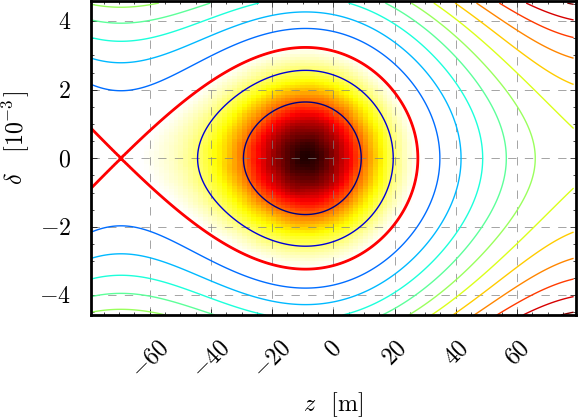
(a) Initial Gaussian bunch

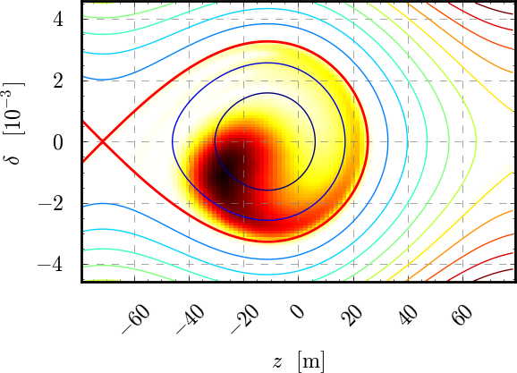
(b) After 2 synchrotron periods

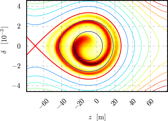
(c) After 6 synchrotron periods

Figure 1: Longitudinal phase space $(z,\delta)$ with $\delta=(p-p_{0})/p_{0}$ during the excitation of the 1:1 dipolar parametric resonance in the PSB (from PyHEADTAIL [6] simulations).

3.2 Implementation in PSB

Based on the current operational LHC-type beam set-up, we introduced the phase modulation at cycle time C575 (corresponding to an intermediate energy of $E_{\text{kin}}=$0.71\text{\,}\mathrm{GeV}$$) in a single harmonic accelerating bucket. During $9\text{\,}\mathrm{ms}$ equivalent to 6 synchrotron periods the beam is driven onto the resonance starting from an initial matched longitudinal emittance of $\epsilon_{z,100\%}=$1.1\text{\,}\mathrm{eV}\text{\,}\mathrm{s}$$. With these settings, the resulting distributions appeared consistently and reproducibly depleted.

Varying the driving frequency for the parametric resonance revealed a broad resonance window. The beam turned out to be correctly excited for frequencies in the range

$$$649\text{\,}\mathrm{Hz}$\leq\frac{\omega_{\text{drive}}}{2\pi}\leq$734\text{\,}\mathrm{Hz}$\quad.$$

This resonance window is sharply defined up to $1\text{\,}\mathrm{Hz}$.

Special attention had to be given to optimise the phase loop gain during the excitation process: for a too strong gain, the phase loop continuously realigns the phase of the main C02 cavities with the beam. This counteracts the excitation and leads to severely perturbed distributions.

Eventually, the long filament can be smoothed to a ring-like phase space distribution by high frequency phase modulation at harmonic $h=9$ with the C16 cavities. Figure 2 shows tomographic reconstructions [8] of longitudinal phase space at important cycle times. The horizontal axis is reverted compared to Fig. 1, since $\phi=-z/R$ with $R$ the machine radius.

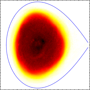
phase $\phi$

energy $E$

(a) PSB C573, before excitation

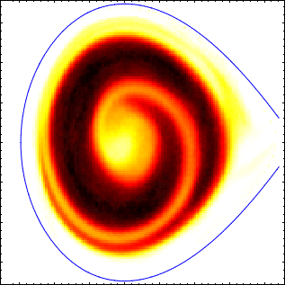
phase $\phi$

energy $E$

(b) PSB C591, after excitation

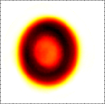
phase $\phi$

energy $E$

(c) PSB C800 ($5\text{\,}\mathrm{ms}$ to extract.)

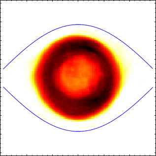
phase $\phi$

energy $E$

(d) PS C171 ($1\text{\,}\mathrm{ms}$ after inject.)

Figure 2: Longitudinal phase space $(\phi,E)$ reconstructed via tomography at different stages in the PSB (measurements).

4 Space Charge Mitigation in PS

To assess the impact of direct space charge during the $1.2\text{\,}\mathrm{s}$ PS injection plateau at $E_{\text{kin}}=$1.4\text{\,}\mathrm{GeV}$$ and $h=7$, we compare single bunch beams of the usual LHC parabolic type with the modified hollow type by measuring transverse emittance blow-up and beam loss. For each shot, tomography and wire scans yield the $z,\delta,x,y$ distributions $15\text{\,}\mathrm{ms}$ after injection and again $20\text{\,}\mathrm{ms}$ before the second batch injection time. Table 1 lists the experiment parameters.

Table 1: Relevant Experiment Beam Parameters for PS

parameter	hollow value	parabolic value
$N$	$(1.66\mathrel{\pm}0.05)\times 10^{12}$	$(1.84\mathrel{\pm}0.03)\times 10^{12}$
$\epsilon_{z,100\%}$	$1.43\pm 0.15\,$\mathrm{eV}\text{\,}\mathrm{s}$$	$1.47\pm 0.11\,$\mathrm{eV}\text{\,}\mathrm{s}$$
$\epsilon_{z,\text{rms}}$	$0.32\mathrel{\pm}0.02\,$\mathrm{eV}\text{\,}\mathrm{s}$$	$0.3\mathrel{\pm}0.01\,$\mathrm{eV}\text{\,}\mathrm{s}$$
$Q_{x},Q_{y}$	$(6.23,6.22)$

Determining the horizontal emittance $\epsilon_{x}$ requires special attention: since the momentum $\delta$ is by construction not Gaussian distributed for hollow bunches, Eq. (2) is not valid. The horizontal particle position is a sum of two independent random variables, $x=x_{\beta}+x_{D_{x}\delta}$. The dispersive profile is given by the measured $\delta$ distribution and $D_{x}=$2.3\text{\,}\mathrm{m}$$ at the wire scanner location. Convolving with a Gaussian distributed betatron profile hence yields an estimate of the horizontal profile. The horizontal emittance $\epsilon_{x}$ can then be found by a least squares algorithm comparing the resulting convolution with the actual measured profile, cf. Fig. 3. This procedure is applied to both beams. Results differ by $24.8\%$ to $34.8\%$ from Eq. (2) in both cases.

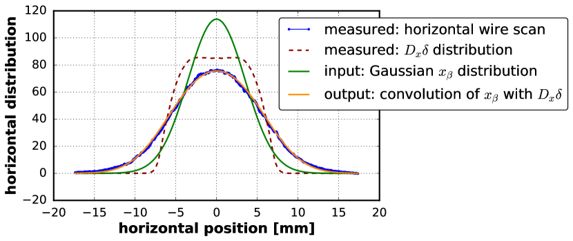
Figure 3: Wire scan comprising betatron and dispersive part.

Over many shots, we vary the bunch length for both beam types by adiabatically ramping the total RF voltage during the initial $15\text{\,}\mathrm{ms}$ to values between the initial $25\text{\,}\mathrm{kV}$ and $80\text{\,}\mathrm{kV}$. Due to varying shot-to-shot efficiency of the C16 blow-up, we achieve total bunch lengths over a range of $B_{L}=130\,..\,$220\text{\,}\mathrm{ns}$$. Figure 4(a) depicts consistently depressed peak line densities by a factor $0.9$ for the flattened profiles compared to the parabolic ones. A theoretically ideal rectangular profile of $4\sigma_{z}$ length would yield a $\sqrt{2\pi}/4\approx 0.63$ depression factor compared to a perfect Gaussian. Both extrema are plotted in Fig. 4(a) for comparison.

We want to compare the impact of space charge for both beam types for fixed $B_{L}$, $N$ and $\epsilon_{u}$. To unify this set in one quantity, we choose to evaluate $\Delta Q_{u}^{\text{max}}$ assuming a 6D Gaussian distributed beam in Eq. (1). Hence we apply (2) as well as using the Gaussian peak line density $\lambda_{\text{max}}=N/(\sqrt{2\pi}\sigma_{z})$ where we set $\sigma_{z}=B_{L}/4$. Figure 4(b) shows how hollow bunches provide statistically significantly lower vertical emittances for the same unified reference tune shift $\Delta Q_{u}^{\text{max}}$. The real tune shift of the hollow bunches is a factor $0.88$ lower due to their reduced $\lambda_{\text{max}}$ and the larger $\sigma_{x}$. In contrast, the parabolic bunches are rather well represented by the Gaussian approach (factor $0.97$ lower real tune shift).

Finally, keeping the maximum RF voltage $80\text{\,}\mathrm{kV}$, we scan the intensity by varying the injected turns in the PSB. Figure 4(c) exhibits the emittance blow-up $\epsilon_{y}^{\text{fin}}/\epsilon_{y}^{\text{ini}}$ versus the brightness, which is again lower for the hollow bunches.

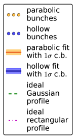
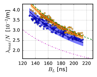
(a) Intensity normalised peak line charge density vs. total bunch length.

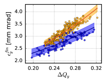
(b) Vertical emittances (end of inject. plateau) vs. space charge tune shift.

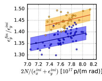
(c) Vertical emittance blow-up vs. brightness (at $V_{\text{rf}}=$80\text{\,}\mathrm{kV}$$).

Figure 4: Comparison of hollow and parabolic bunches. Fits include $1\sigma$ confidence bands.

5 Conclusion

We have set up a reliable process to create hollow bunches with minimal changes to the operational PSB cycle. Due to the lower peak line density, the longitudinally hollow bunches are shown to be less affected by space charge compared to the LHC-type parabolic bunches during the PS injection plateau.

6 Acknowledgement

The PSB feedback systems have been set up to create and transfer hollow bunches owing to the invaluable support by Maria-Elena Angoletta and Michael Jaussi.

References

- [1] R. Wasef et al., “Space Charge Effects and Limitations in the CERN Proton Synchrotron”, in Proc. 4th Int. Particle Accelerator Conf. (IPAC’13), Shanghai, China, May 2013, paper WEPEA070, pp. 2669-2671.
- [2] R. Cappi, R. Garoby, S. Hancock, M. Martini, J.P. Riunaud, “Measurement and Reduction of Transverse Emittance Blow-up Induced by Space Charge Effects”, in Proc. 15th IEEE Particle Accelerator Conf. (PAC’93), Washington, DC, USA, May 1993, pp. 3570-3572.
- [3] R. Garoby, S. Hancock, “New Techniques for Tailoring Longitudinal Density in a Proton Synchrotron”, in Proc. 4th European Particle Accelerator Conf. (EPAC’94), London, UK, June 1994, pp. 282.
- [4] K. Schindl, “Space Charge”, CERN/PS 99-012(DI), 1999.
- [5] H. Huang et al., “Experimental Determination of the Hamiltonian for Synchrotron Motion with RF Phase Modulation”, in Phys. Rev. E, vol. 48, no. 6, Dec. 1993, pp. 4678-4688.
- [6] E. Metral et al., “Beam Instabilities in Hadron Synchrotrons”, in IEEE Transactions on Nuclear Science, vol. 63, no. 2, Apr. 2016, pp. 1001-1050.
- [7] A. Oeftiger, “Space Charge Effects and Advanced Modelling for CERN Low Energy Machines”, unpublished Ph.D. thesis, LPAP, EDPY, École Polytechnique Fédérale de Lausanne, Lausanne, Switzerland, 2016.
- [8] S. Hancock, S.R. Koscielniak, M. Lindroos, “Longitudinal Phase Space Tomography with Space Charge”, in Proc. 7th European Particle Accelerator Conf. (EPAC 2000), Vienna, Austria, July 2000, pp. 1726-1728.