Membrane Matrix models and non-perturbative checks of gauge/gravity duality

Abstract:

We compare the bosonic and maximally supersymmetric membrane models. We find that in Hoppe regulated form the bosonic membrane is well approximated by massive Gaussian quantum matrix models. In contrast the similarly regulated supersymmetric membrane, which is equivalent to the BFSS model, has a gravity dual description. We sketch recent progress in checking gauge/gravity duality in this context.

1 Introduction

The proposal that there is a gravitational dual to gauged matter systems represents a dramatic insight into certain non-perturbative phenomena. The simplest known models with gravitational duals are quantum mechanical models with extended supersymmetry and the simplest of these is the model with maximal supersymmetry now known as the BFSS model [1]. Though the model itself arose initially in the context of supersymmetric quantum mechanical models [2, 3, 4], it subsequently emerged from the matrix regularisation of membranes introduced by Hoppe [5] and extended to the supermembrane in [6] and [7]. It is this quantisation of membranes that is our focus here. The BFSS model was proposed as a non-perturbative formulation of M-theory which in the infinite matrix size limit is conjectured to capture the entire dynamics of M-theory.

In Hoppe’s regularisation of membranes what remains of the original diffeomorphism invariance of the membrane action is an $SU(N)$ gauge symmetry. The model has a single dimensionful coupling constant. When placed in a thermal bath the coupling can be absorbed into the fields and the temperature, to define a dimensionless temperature. At high temperature the inverse of the dimensionless temperature plays the rôle of a small parameter and the model is in a perturbative regime. On the contrary at low temperature the the model becomes strongly coupled.

In the low temperature regime the bosonic model turns out [8] to be well described by a massive quantum matrix model while the supersymmetric model is described by a dual geometry [9] which is a solution to IIA supergravity and can be lifted to a solution to 11-d supergravity. For the thermal system the gravity dual has a black hole whose Hawking-temperature is that of the thermal bath.

A more complicated example that was designed to describe the M2-brane in a background longitudinal M5-brane is the Berkooz-Douglas model [10]. The model also arises naturally in string theory as the effective low energy description of a D0/D4-brane system. The D0-branes give rise to the adjoint fields of the pure BFSS model, while the D4-branes are described by fundamental hypermultiplets. In the large $N$ limit at strong ’t Hooft coupling the model has a supergravity dual description. The best understood regime of this duality is when the number of D4-branes is much smaller than the number of D0-branes, which from a field theory point of view corresponds to the quenched approximation. In this limit the D0-branes are described by the supergravity dual of the BFSS model, while the D4-branes are treated as Dirac–Born–Infeld probes. The model was successfully simulated in ref. [11], where excellent agreement between field theory and supergravity has been found.

We will review some recent progress in checking this duality and explain its significance to a non-perturbative formulation of M-theory.

2 Hoppe Regularised Membranes

The Membrane action, with metric signature $(-,+,..+)$, in Polyakov form is given by

$$S=-\frac{T}{2\Lambda}\int d^{3}\sigma\sqrt{-h}\left(h^{\alpha\beta}\partial_{\alpha}X^{\mu}\partial_{\beta}X^{\nu}\eta_{\mu\nu}-\Lambda\right)\qquad\hbox{with }\quad T=\frac{1}{(2\pi)^{2}{\it l}_{p}^{3}}\;.$$ (1)

Varying with respect to $h_{\alpha\beta}$ one obtains

$$\frac{1}{2}h_{\gamma\delta}(h^{\alpha\beta}G_{\alpha\beta}-\Lambda)=G_{\gamma\delta}\;,\quad\hbox{tracing gives }\quad h^{\alpha\beta}G_{\alpha\beta}=3\Lambda\;,\quad\hbox{so }\Lambda\;h_{\gamma\delta}=G_{\gamma\delta}\;.$$ (2)

Then substituting into (1) gives the standard Nambu-Goto form

$$S=-T\int d^{3}\sigma\sqrt{-G}\;.$$ (3)

Alternatively, instead of going to the Nambu-Goto form of the action, we can gauge away some of its components of $h_{\alpha\beta}$ and attempt to solve the resulting constraints on the embedding coordinates. When the membrane topology is restricted to ${\mathbb{R}}\times\Sigma$ we can use the gauge $h_{0i}=0$ and $h_{00}=-\frac{4}{\Lambda\rho^{2}}{\rm det}(G_{ij})$ so we have the constraint

$$\partial_{t}X^{\mu}\partial_{i}X^{\nu}\eta_{\mu\nu}=0\quad\hbox{and}\quad\Lambda\;h_{00}=\partial_{t}X^{\mu}\partial_{t}X^{\mu}\eta_{\mu\nu}=-\frac{4}{\rho^{2}}{\rm det}(G_{ij})\ .$$ (4)

Using light-cone coordinates with $X^{\pm}=(X^{0}\pm X^{D-1})/\sqrt{2}$ and choosing $X^{+}=\tau$ we see that the constraints take the form

$$\partial_{i}X^{-}=(\partial_{\tau}X^{a})(\partial_{i}X_{a})\quad\hbox{and}\quad\partial_{\tau}X^{-}=\frac{1}{2}\partial_{\tau}X^{a}\partial_{\tau}X_{a}+\frac{2}{\rho^{2}}{\rm det}(G)$$ (5)

with the action

$$S=\frac{T\rho}{4}\int dtd^{2}\sigma\left(\dot{X}^{\mu}\dot{X}^{\nu}\eta_{\mu\nu}-\frac{4}{\rho^{2}}{\rm det}(G_{ij})\right)\ .$$

An important observation is that in two dimensions ${\rm det}(G_{ij})$ can be rewritten using $\{f,g\}=\epsilon^{ij}\partial_{i}f\partial_{j}g$ so that

$$S=\frac{T\rho}{4}\int dtd^{2}\sigma\left(\dot{X}^{\mu}\dot{X}^{\nu}\eta_{\mu\nu}-\frac{4}{\rho^{2}}\{X^{\mu},\,X^{\nu}\}^{2}\right)$$

and the constraints become

$$\dot{X}^{\mu}\partial_{i}X_{\mu}=0\implies\{\dot{X}^{\mu},\,X_{\mu}\}=0\quad{\rm and}\quad\dot{X}^{\mu}\dot{X}_{\mu}=-\frac{2}{\rho^{2}}\{X^{\mu},\,X^{\nu}\}\{X_{\mu},\,X_{\nu}\}\,.$$ (6)

In light-cone coordinates the Lagrangian is linear in the momentum $P_{-}$ and a Legendre transform to the Hamiltonian gives

$$S=-T\int\sqrt{-G}\longrightarrow H=\int\left(\frac{1}{\rho T}P^{a}P^{a}+\frac{T}{2\rho}\{X^{a},\,X^{b}\}^{2}\right)\;,$$

with the remaining constraint $\{P^{a},\,X^{a}\}=0$.

This model is still not fully tractable, however Hoppe then made the observation that if he treated the membrane surface as a quantum phase space one could use a matrix regularisation of the membrane. In this scheme functions on the membrane world-volume at fixed time, $f(\sigma^{1},\,\sigma^{2})$ are replaced by $N\times N$ matrices, $f\rightarrow F$, with the matrices providing a discrete approximation to the corresponding functions. This is the same procedure as is used in the fuzzy approach [14] with the significant difference that the geometry of $\Sigma$, the membrane surface, is lost.

The quantum Hamiltonian then reads

$${\rm H}=-\frac{1}{2}\nabla^{2}-\frac{1}{4}\sum_{i,j=1}^{p}{\rm Tr}[X^{i},\,X^{j}]^{2}$$

and the constraint requires that observables are restricted to $SU(N)$ invariants. The model describes a quantised “fuzzy” relativistic membrane in $p+1$ dimensions.

The Euclidean finite temperature action for the model is

$$S_{b}=\frac{1}{g^{2}}\,\int_{0}^{\beta}dt\,{\rm tr}\left\{\frac{1}{2}({\cal D}_{t}{X^{i}})^{2}-\frac{1}{4}[X^{i},\,X^{j}]^{2}\right\}\ .$$ (7)

where ${\cal D}_{t}{X^{i}}=\partial_{t}X^{i}+[A,\,X^{i}]$ and $\beta$, the period of the $S^{1}$, is the inverse temperature. Since the theory is one dimensional the only physical content of the gauge field is its holonomy around the $S^{1}$. It is also the high temperature limit of a $1+1$ dimensional ${\cal N}=8$ supersymmetric Yang-Mills theory on ${\bf R}\times S^{1}$ where $\beta$ is now the period of a spatial $S^{1}$ (not the inverse temperature) and the fermions drop out due to their anti-periodic boundary conditions at finite temperature [15].

This model has been studied in some detail both non-perturbatively [16, 8] and using a $1/p$ expansion [8, 17, 18] where $p$ is the spatial dimension into which the membrane is embedded. It was found that as the temperature is decreased the model first undergoes a 2nd order deconfining-confining phase transition into a phase with non-uniform but gapless distribution for the holonomy. As the temperature is further decreased there is a 3rd order transition to a gapped holonomy with a quadratic decrease in the internal energy to a constant value for lower temperatures. The high temperature expansion of the model was developed in [19]. In [8] it was found that the low temperature phase of the model has an effective description in terms of free massive scalars which captures many of the finite temperature features of the model including one of its two phase transitions.

For the purposes of the discussion here the zero temperature aspects of the model are most interesting. In this case, the gauge field which in the static gauge enters only as a holonomy at finite temperature, can be completely gauged away and the model simplifies. Furthermore, at zero temperature the correlator:

$$\left\langle{\rm Tr}\left(X^{1}(0)\,X^{1}(t)\right)\right\rangle\propto e^{-m\,t}+\dots\ ,$$ (8)

captures the gap $m=E_{1}-E_{0}$ of the theory. To calculate the gap in the discrete theory, we periodically identify the time direction with period $\beta$:

$$\left\langle{\rm Tr}\left(X^{1}(0)\,X^{1}(t)\right)\right\rangle=A\,(e^{-m\,t}+e^{-m(\beta-t)})\ ,$$ (9)

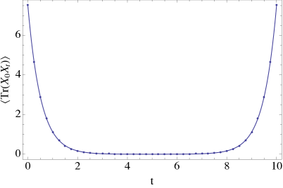
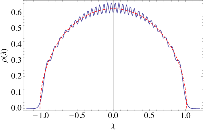
Note that although formally $\beta$ is the same parameter that we have at finite temperature, since we set the holonomy to zero here its meaning is just a periodic coordinate as opposed to inverse temperature. Our result for the correlator for $N=30$, $\beta=10$ and lattice spacing $a=0.25$ is presented on the left in Figure 1. The fitting curve is given by equation (9) and when we perform a two parameter fit we obtain $A\approx 7.50\pm 0.2$ and $m\approx(1.90\pm.01)\,\lambda^{1/3}\,$. However, for Gaussian scalar fields of mass $m$ we have $A=\frac{N}{2m(1-{\rm e}^{-\beta m})}$ and performing a one parameter fit for $m$ yields $m=1.965\pm 0.007$ and $A=7.63\pm 0.03$. On the right we have presented a plot of the eigenvalue distribution of one of the matrices for the same parameters. The fitting curve represents a Wigner semicircle of radius $R_{\lambda}\approx 1.01$. The fact that the theory is gapped and that the eigenvalue distribution is a semicircle suggests that that at low temperate the model has an effective action:

Figure 1: On the left: A plot of the correlator $\left\langle{\rm Tr}\left(X^{1}(0)\,X^{1}(t)\right)\right\rangle$ for $N=30$, $\beta=10$ and lattice spacing $a=0.25$. The fitting curve is given by equation (2.9) with $A=\frac{N}{2m(1-{\rm e}^{-\beta m})}$ and with parameters $m\approx(1.965\pm.007)\lambda^{1/3}\,$. On the right: A plot of the eigenvalue distribution of one of the scalars for the same parameters. The fitting curve represent a Wigner-semicircle of radius $R_{\lambda}\approx 1.01\,$.

$$S_{\rm eff}=N\int\limits_{-\infty}^{\infty}dt\,{\rm Tr}\left(\frac{1}{2}\left(\dot{X}^{i}\right)^{2}+\frac{1}{2}m^{2}\left(X^{i}\right)^{2}\right)$$ (10)

for each of the matrices $X^{i}$. It is well known [20] that for the action (10) the eigenvalue distribution of $X$ is given by a Wigner semicircle of radius:

$$R_{\lambda}=\sqrt{\frac{2}{m}}\approx 1.009\pm.002,$$ (11)

where we have substituted $m\approx 1.965\pm.007$. This agrees nicely (within errors) with the result for $R_{\lambda}\approx 1.01$ obtained by fitting the actual distribution. It is also in excellent agreement with the large $p$ theoretical prediction of [17],

$$R_{\lambda}(p)=\sqrt{\frac{2}{p^{1/3}}}\left(1+\frac{1}{p}\left(\frac{7\sqrt{5}}{30}-\frac{9}{32}\right)+\cdots\right)\simeq 1.0068$$ (12)

Numerical simulations of the gauged massive Gaussian model show that it too has a phase transition (there is only one rather than the two of the full model) and that when the mass is tuned to the value of the full model the transition temperature is almost identical [8].

That the Hoppe quantised bosonic membrane has a mass gap was clear from the analysis of [21], the new ingredient here is putting a value on this mass and demonstrating how closely the model is to a gauged massive Gaussian model.

2.1 Quantum Gravity from matrices

It has been argued [22] that at short distances due to quantum gravity the spatial coordinates, $X^{a}$ should not commute i.e. $[X^{a},\,X^{b}]\neq 0$ somewhat in analogy with the non-commutativity of phase space, but putting this non-commutativity to a spacetime independent quantity, e.g. $[X^{a},\,X^{b}]=i\,\theta^{ab}$ breaks rotational invariance. One would wish to have the non-commutativity be a feature of the high energy theory and disappear at low energies. If one takes each $X^{a}$ to be an $N\times N$ matrix (as in matrix mechanics) and tries

$$H_{0}={\rm Tr}\left(\frac{1}{2}\sum_{a=1}^{p}\dot{X}^{a}\dot{X}^{a}-\frac{1}{4}\sum_{a,b=1}^{p}[X^{a},\,X^{b}][X^{a},\,X^{b}]\right)$$ (13)

one can see that the bottom of the potential has $[X^{a},\,X^{b}]=0$ and one might hope that at low energy the matrices would effectively commute. However, as we saw above the model becomes massive at low energies and the minimum is pushed upwards so that the non-commutativity does not disappear. The $X_{a}$ are always described (see Figure 1) by a Wigner semi-circle.

Following arguments similar to those above, Polchinski argues [23] that one might suspect that the model still has something to do with quantum gravity and that the missing ingredient is supersymmetry. The model can be made supersymmetric by adding a fermionic degree of freedom for each bosonic degree of freedom so that

$$H_{1}={\rm Tr}\left(\frac{1}{2}\sum_{a=1}^{p}\dot{X}^{a}\dot{X}^{a}-\frac{1}{4}\sum_{a,a=1}^{p}[X^{a},\,X^{a}][X^{a},\,X^{a}]+\frac{1}{2}\Theta^{T}\gamma^{i}[X^{a},\,\Theta]\right)$$ (14)

with the Fermions quantised as $\{{\Theta_{\alpha}}_{i}^{j},\,{\Theta_{\beta}}_{k}^{l}\}=\delta_{\alpha\beta}\delta_{ik}\delta^{jl}$, i.e. as Clifford algebra elements or equivalently as fermionic Majorana oscillators. It was observed in [2] that one can only match fermions with bosons if $p=2,3,5$ or $9$.

The potential is invariant under the global $SU(N)$ transformations $X^{a}\rightarrow UX^{a}U^{-1}$, so promoting this symmetry to a gauge symmetry with $U=U(t)$ and $\dot{X}^{a}\rightarrow D_{t}X^{a}=\dot{X}^{a}+i[A,\,X^{a}]$ where $A$ is the $SU(N)$ gauge field gives the matrix regularisation of the supermembrane [6]. The constraint of supersymmetry then means that supersymmetric membranes only exist in spacetime dimensions $4$, $5$, $7$ and $11$.

3 The BFSS model

Matrix supermembranes propagating in $p+2$ dimensions coincide with $p+1$-dim $SU(N)$ supersymmetric Yang-Mills theory dimensionally reduced to one dimension (only time dependence). The BFSS model, $p=9$, also describes a system of N interacting D0 branes.

3.1 The Hamiltonian Formulation

The $16$ supercharges:

$$Q_{\beta}=Tr\left(\frac{1}{2}\Theta_{\alpha}\gamma^{a}_{\alpha\beta}P_{a}+\frac{i}{4}\Theta_{\alpha}\gamma^{ab}_{\alpha\beta}[X_{a},X_{b}]\right)$$

$$\{Q_{\alpha},Q_{\beta}\}=\delta_{\alpha\beta}{\cal H}+\gamma^{a}_{\alpha\beta}Tr(X^{a}J)$$

give the Hamiltonian:

$${\rm H}=Tr\left(\frac{1}{2}P^{a}P^{a}-\frac{1}{4}[X^{a},X^{b}]^{2}+\frac{1}{2}\Theta^{T}\gamma^{a}[\Theta,X^{a}]\right)\ ,$$

where $J$ is the generator of $SU(N)$ and is zero on physical states

$$J=i[P^{b},X^{b}]+\Theta_{\alpha}\Theta_{\alpha}-\delta_{\alpha\alpha}\frac{N^{2}-1}{2N}\;.$$

The 16 fermionic matrices $\Theta_{\alpha}=\Theta_{\alpha A}t^{A}$ are quantised as ${\Theta_{\alpha A},\Theta_{\beta B}}=2\delta_{\alpha\beta}\delta_{AB}$. The $\Theta_{\alpha A}$ are $2^{8(N^{2}-1)}$ and the Fermionic Hilbert space is

$${\cal H}^{F}={\cal H}_{256}\otimes\cdots\otimes{\cal H}_{256}$$

with ${\cal H}_{256}={\bf 44}\oplus{\bf 84}\oplus{\bf 128}$ suggestive of the graviton, anti-symmetric tensor and gravitino of $11$-dimensional supergravity. For an attempt to find the ground state if this Hamiltonian see ref. [25].

3.2 Lagrangian formulation

The easiest way to obtain the BFSS matrix model is via dimensional reduction of ten dimensional supersymmetric Yang-Mills theory down to one dimension. The resulting reduced ten dimensional action is given by

$$S_{M} =\frac{1}{g^{2}}\int dt\,{\rm Tr}\left\{\frac{1}{2}({\cal D}_{0}X^{i})^{2}+\frac{1}{4}[X^{i},X^{j}]^{2}-\frac{i}{2}\Psi^{T}C_{10}\,\Gamma^{0}D_{0}\Psi+\frac{1}{2}\Psi^{T}C_{10}\,\Gamma^{i}[X^{i},\Psi]\right\}\ ,$$ (15)

where $\Psi$ is a thirty two component Majorana–Weyl spinor, $\Gamma^{\mu}$ are ten dimensional gamma matrices and $C_{10}$ is the charge conjugation matrix satisfying $C_{10}\Gamma^{\mu}C_{10}^{-1}=-{\Gamma^{\mu}}^{T}$.

4 The gravity dual

Since the BFSS model describes the dynamics of D0-branes gauge/gravity dualtiy gives predictions for the strong coupling regime of the theory. To access these predictions one needs to look at the supergravity. Also, since the supermembrane is meant as the basic ingredient of M-theory and in analogy with string theory where quantised superstrings gives 10-dimensional supergravities as their low energy theories, the supermembrane is expected to give 11-dimensional supergravity as its low energy theory. It turns out that the dual geometry for the BFSS model can be lifted to a solution to 11-dimensional supergravity. We briefly describe the solution in this context.

The bosonic action for eleven-dimensional supergravity is given by:

$$S_{11D}=\frac{1}{2\kappa_{11}^{2}}\int\left[\sqrt{-g}R-\frac{1}{2}F_{4}\wedge*F_{4}-\frac{1}{6}A_{3}\wedge F_{4}\wedge F_{4}\right]\ ,$$ (16)

where $2\kappa_{11}^{2}=16\pi G_{N}^{11}=\frac{(2\pi l_{p})^{9}}{2\pi}$. With the equations of motion of this system being:

$$R_{MN}-\frac{1}{2}g_{MN}R=\frac{1}{2}F^{2}_{MN}-\frac{1}{4}g_{MN}|F_{4}|^{2}$$ (17)

$$d*F_{4}+\frac{1}{2}F_{4}\wedge F_{4}=0,\qquad dF_{4}=0.$$ (18)

Dimensionally reducing on $S^{1}$ gives us IIA supergravity. The reduction is specified by:

$$g_{MN}^{11}dx^{M}dx^{N}={\rm e}^{-\frac{2}{3}\Phi}g_{mn}^{10}dx^{m}dx^{n}+{\rm e}^{\frac{4}{3}\Phi}(dx_{10}+C_{m}dx^{m})^{2}$$ (19)

$$A_{10mn}dx^{m}\wedge dx^{n}=\frac{B_{2}}{2\pi R}\qquad A_{lmn}dx^{l}\wedge dx^{m}\wedge dx^{n}=C_{3}\ ,$$ (20)

where the constant giving the string coupling has been removed from the dilaton. Then with $2\kappa_{0}^{2}g_{s}^{2}=\frac{2\kappa_{11}^{2}}{2\pi R}$, where $R$ is the radius of the $X_{10}$ circle on which the compactification is done, one obtains the IIA supergravity action.

The leading $\alpha^{\prime}=l_{s}^{2}$ low energy effective field theory on the dual gravity side is given by IIA supergravity the bosonic part of whose action is given in the string frame by:

$$S_{IIA}=\frac{1}{2\kappa_{0}^{2}g_{s}^{2}}\int d^{10}x\sqrt{-g}\left\{{\rm e}^{-2\Phi}[R+4|d\phi|^{2}-\frac{1}{12}|H_{3}|^{2}-\frac{1}{4}|G_{2}|^{2}-\frac{1}{48}|G_{4}|^{2}]\right\}+\frac{1}{4\kappa_{0}^{2}}\int B_{2}\wedge dC_{3}\wedge dC_{3}\;,$$

where

$$H_{3}=dB_{2}\;,\qquad G_{2}=dC_{1}\;,\qquad G_{4}=dC_{3}+H_{3}\wedge C_{1}\ .$$

Eleven dimensional supergravity is the natural strong coupling limit of the IIA superstring. The fields $(\phi,g_{mn},B_{mn})$ are from the $NS\otimes NS$ sector of the IIA string while the fields $(C_{1},C_{3})$ are from the $R\otimes R$ sector.

The relevant solution to eleven dimensional supergravity for the dual geometry to the BFSS model corresponds to $N$ coincident $D0$ branes in the IIA theory. It is given by:

$$ds^{2}=-H^{-1}dt^{2}+dr^{2}+r^{2}d\Omega_{8}^{2}+H(dx_{10}-Cdt)^{2}$$

with $A_{3}=0$.

The one-form is given by $C=H^{-1}-1$ and $H=1+\frac{\alpha_{0}N}{r^{7}}$, where $\alpha_{0}=(2\pi)^{2}14\pi g_{s}l_{s}^{7}$. After reducing to ten dimensions and taking near horizon limit (with $U=r/\alpha^{\prime}$) the metric becomes [9]:

$$ds^{2}=\alpha^{\prime}\left(-\frac{F}{\sqrt{H}}dt^{2}+\frac{\sqrt{H}}{F}dU^{2}+\sqrt{H}U^{2}d\Omega_{8}\right)\ ,$$ (21)

where $H(U)=\frac{240\pi^{5}\lambda}{U^{7}}$ and the black hole time dilation factor is $F(U)=1-\frac{U_{0}^{7}}{U^{7}}$, where $U_{0}$ is the radius of the horizon related to the Hawking temperature:

$$\frac{T}{\lambda^{1/3}}=\frac{1}{4\pi\lambda^{1/3}}H^{-1/2}F^{\prime}(U_{0})=\frac{7}{2^{4}15^{1/2}\pi^{7/2}}{\left(\frac{U_{0}}{\lambda^{1/3}}\right)}^{5/2}.$$ (22)

Then from black hole thermodynamics the predictions for the entropy and energy are:

$$\frac{S}{N^{2}}=\frac{1}{N^{2}}\frac{A}{4G_{N}}=4^{\frac{13}{5}}15^{\frac{2}{5}}\left(\frac{\pi}{7}\right)^{\frac{14}{5}}{\left(\frac{T}{\lambda^{1/3}}\right)}^{9/2}\implies\frac{E}{\lambda^{1/3}N^{2}}=\left(\frac{2^{21}3^{12}5^{2}}{7^{19}}\pi^{14}\right)^{1/5}{\left(\frac{T}{\lambda^{1/3}}\right)}^{14/5}$$ (23)

5 Non-perturbative Field Theory Results

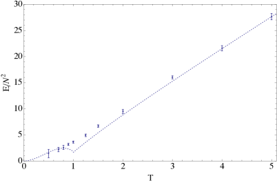
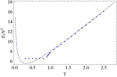
To illustrate the difference between the bosonic membrane and its supersymmetric relative in the eleven dimensional theory we show the expectation value of the energy, i.e. $\langle H\rangle/N^{2}$ given by

$$E/N^{2} = \left\langle-\frac{3}{4N\beta}\int\limits_{0}^{\beta}d\tau\,{\rm Tr}\left([X^{i},X^{j}]^{2}\right)\right\rangle$$ (24)

while for the BFSS model the energy has a fermionic component and is given by

$$E/N^{2} = \left\langle-\frac{3}{4N\beta}\int_{0}^{\beta}d\tau\;{\rm Tr}\left([X^{i},X^{j}]^{2}+\Psi^{T}C_{10}\,\Gamma^{i}[X^{i},\Psi]\right)\right\rangle\,.$$ (25)

We show the measured values of the two energies in Figure 2.

Figure 2: On the left: Results for the internal energy extrapolated from simulations with $8\leq N\leq 14$ and $8\leq\Lambda\leq 16$. The dashed curve at high temperature correspond to the theoretical results of [19], while the low temperature curve represent the prediction for the internal energy from the gauge/gravity correspondence [26]. On the right: Plots of the scaled energy $E/N^{2}$ of the bosonic model as functions of the temperature. The dashed curve corresponds to the high temperature behaviour obtained in [19]. One can see that near $T\approx 0.9$ the plots suggest the existence of a second order phase transition. The energy and temperature in the plots are in units of $\lambda^{1/3}$.

When $1/\alpha^{\prime}$ corrections are included, the data converges on the low temperature prediction of the gauge/gravity correspondence. Our results on the BFSS model [8] agree well with those of the other groups that have simulated the system  [27]  [28],  [29].

6 Conclusions

• Bosonic membranes when quantised are massive $m\simeq{p}^{1/3}l_{p}$ and well approximated by a set of $p$ massive Gaussian matrix models.

• Supersymmetric membranes are highly non-trivial with infra-red divergences. Gauge/gravity predictions are in excellent agreement with non-perturbative tests and the interpretation as a non-perturbative formulation of $M$-theory is promising.