Observational-Interventional Priors for Dose-Response Learning

Abstract

Controlled interventions provide the most direct source of information for learning causal effects. In particular, a dose-response curve can be learned by varying the treatment level and observing the corresponding outcomes. However, interventions can be expensive and time-consuming. Observational data, where the treatment is not controlled by a known mechanism, is sometimes available. Under some strong assumptions, observational data allows for the estimation of dose-response curves. Estimating such curves nonparametrically is hard: sample sizes for controlled interventions may be small, while in the observational case a large number of measured confounders may need to be marginalized. In this paper, we introduce a hierarchical Gaussian process prior that constructs a distribution over the dose-response curve by learning from observational data, and reshapes the distribution with a nonparametric affine transform learned from controlled interventions. This function composition from different sources is shown to speed-up learning, which we demonstrate with a thorough sensitivity analysis and an application to modeling the effect of therapy on cognitive skills of premature infants.

1 Contribution

We introduce a new solution to the problem of learning how an outcome variable $Y$ varies under different levels of a control variable $X$ that is manipulated. This is done by coupling different Gaussian process priors that combine observational and interventional data. The method outperforms estimates given by using only observational or only interventional data in a variety of scenarios and provides an alternative way of interpreting related methods in the design of computer experiments.

Many problems in causal inference [15] consist of having a treatment variable $X$ and and outcome $Y$, and estimating how $Y$ varies as we control $X$ at different levels. If we have data from a randomized controlled trial, where $X$ and $Y$ are not confounded, many standard modeling approaches can be used to learn the relationship between $X$ and $Y$. If $X$ and $Y$ are measured in an observational study, the corresponding data can be used to estimate the association between $X$ and $Y$, but this may not be the same as the causal relationship of these two variables because of possible confounders.

To distinguish between the observational regime (where $X$ is not controlled) and the interventional regime (where $X$ is controlled), we adopt the causal graphical framework of [17] and [20]. In Figure 1 we illustrate the different regimes using causal graphical models. We will use $p(\cdot\ |\ \cdot)$ to denote (conditional) density or probability mass functions. In Figure 1(a) we have the observational, or “natural,” regime where common causes $\mathbf{Z}$ generate both treatment variable $X$ and outcome variable $Y$. While the conditional distribution $p(Y=x\ |\ X=x)$ can be learned from this data, this quantity is not the same as $p(Y=y\ |\ do(X=x))$: the latter notation, due to Pearl [17], denotes a regime where $X$ is not random, but a quantity set by an intervention performed by an external agent. The relation between these regimes comes from fundamental invariance assumptions: when $X$ is intervened upon, “all other things are equal,” and this invariance is reflected by the fact that the model in Figure 1(a) and Figure 1(b) share the same conditional distribution $p(Y=x|X=x,\mathbf{Z}=\mathbf{z})$ and marginal distribution $p(\mathbf{Z}=\mathbf{z})$. If we observe $\mathbf{Z}$, $p(Y=y\ |\ do(X=x))$ can be learned from observational data, as we explain in the next section.

(a)	(b)	(c)

Figure 1: Graphs representing causal graphical models. Circles represent random variables, squares represent fixed constants. (a) A system where $\mathbf{Z}$ is a set of common causes (confounders), common parents of $X$ and $Y$ here represented as a single vertex. (b) An intervention overrides the value of $X$ setting it to some constant. The rest of the system remains invariant. (c) $Z_{O}$ is not a common cause of $X$ and $Y$, but blocks the influence of confounder $Z_{H}$.

Our goal is to learn the relationship

$$f(x)\equiv\mathbb{E}[Y\ |\ do(X=x)],x\in\mathcal{X},$$ (1)

where $\mathcal{X}\equiv\{x_{1},x_{2},\dots,x_{T}\}$ is a pre-defined set of treatment levels. We call the vector $f(\mathcal{X})\equiv[f(x_{1});\dots;f(x_{T})]^{\top}$ the response curve for the “doses” $\mathcal{X}$. Although the term “dose” is typically associated with the medical domain, we adopt here the term dose-response learning in its more general setup: estimating the causal effect of a treatment on an outcome across different (quantitative) levels of treatment. We assume the causal structure information is known, complementing approaches for causal network learning [20, 10] by tackling the quantitative and statistical side of causal prediction.

In Section 2, we provide the basic notation of our setup. Section 3 describes our model family. Section 4 provides a thorough set of experiments assessing our approach, including sensitivity to model misspecification. We provide final conclusions in Section 5.

2 Background

The target estimand $p(Y=y\ |\ do(X=x))$ can be derived from the structural assumptions of Figure 1(b) by standard conditioning and marginalization operations:

$$p(Y=y\ |\ do(X=x))=\int p(Y=y\ |\ X=x,\mathbf{Z}=\mathbf{z})p(\mathbf{Z}=\mathbf{z})\ d\mathbf{z}.$$ (2)

Notice the important difference between the above and $p(Y=y\ |\ X=x)$, which can be derived from the assumptions in Figure 1(a) by marginalizing over $p(\mathbf{Z}=\mathbf{z}\ |\ X=x)$ instead. The observational and interventional distributions can be very different. The above formula is sometimes known as the back-door adjustment [17] and it does not require measuring all common causes of treatment and outcome. It suffices that we measure variables $\mathbf{Z}$ that block all “back-door paths” between $X$ and $Y$, a role played by $Z_{O}$ in Figure 1(c). A formal description of which variables $\mathbf{Z}$ will validate (2) is given by [21, 17, 20]. We will assume that the selection of which variables $\mathbf{Z}$ to adjust for has been decided prior to our analysis, although in our experiments in Section 4 we will assess the behavior of our method under model misspecification. Our task is to estimate (1) nonparametrically given observational and experimental data, assuming that $\mathbf{Z}$ satisfies the back-door criteria.

One possibility for estimating (1) from observational data $\mathcal{D}_{obs}\equiv\{(Y^{(i)},X^{(i)},\mathbf{Z}^{(i)})\}$, $1\leq i\leq N$, is by first estimating $g(x,\mathbf{z})\equiv\mathbb{E}[Y\ |\ X=x,\mathbf{Z}=\mathbf{z}]$. The resulting estimator,

$$\hat{f}(x)\equiv\frac{1}{N}\sum_{i=1}^{N}\hat{g}(x,\mathbf{z}^{(i)}),$$ (3)

is consistent under some general assumptions on $f(\cdot)$ and $g(\cdot,\cdot)$. Estimating $g(\cdot,\cdot)$ nonparametrically seems daunting, since $\mathbf{Z}$ can in principle be high-dimensional. However, as shown by [6], under some conditions the problem of estimating $\hat{f}(\cdot)$ nonparametrically via (3) is no harder than a one-dimensional nonparametric regression problem. There is however one main catch: while observational data can be used to choose the level of regularization for $\hat{g}(\cdot)$, this is not likely to be an optimal choice for $\hat{f}(\cdot)$ itself. Nevertheless, even if suboptimal smoothing is done, the use of nonparametric methods for estimating causal effects by back-door adjustment has been successful. For instance, [8] uses Bayesian classification and regression trees for this task.

Although of practical use, there are shortcomings to this idea even under the assumption that $\mathbf{Z}$ provides a correct back-door adjustment. In particular, Bayesian measures of uncertainty should be interpreted with care: a fully Bayesian equivalent to (3) would require integrating over a model for $p(\mathbf{Z})$ instead of the empirical distribution for $\mathbf{Z}$ in $\mathcal{D}_{obs}$; evaluating a dose $x$ might require combining many $g(x,\mathbf{z}^{(i)})$ where the corresponding training measurements $x^{(i)}$ are far from $x$, resulting on possibly unreliable extrapolations with poorly calibrated credible intervals. While there are well established approaches to deal with this “lack of overlap” problem in binary treatments or linear responses [19, 9], it is less clear what to do in the continuous case with nonlinear responses.

In this paper, we focus on a setup where it is possible to collect interventional data such that treatments are controlled, but where sample sizes might be limited due to financial and time costs. This is related to design of computer experiments, where (cheap, but biased) computer simulations are combined with field experiments [2, 7]. The key idea of combining two sources of data is very generic, the value of new methods being on the design of adequate prior families. For instance, if computer simulations are noisy, it is may not be clear how uncertainty at that level should be modeled. We leverage knowledge of adjustment techniques for causal inference, so that it provides a partially automated recipe to transform observational data into informed priors. We leverage knowledge of the practical shortcomings of nonparametric adjustment (3) so that, unlike the biased but low variance setup of computer experiments, we try to improve the (theoretically) unbiased but possibly oversmooth structure of such estimators by introducing a layer of pointtwise affine transformations.

Heterogeneous effects and stratification. One might ask why marginalize $\mathbf{Z}$ in (2), as it might be of greater interest to understand effects at the finer subpopulation levels conditioned on $\mathbf{Z}$. In fact, (2) should be seen as the most general case, where conditioning on a subset of covariates (for instance, gender) will provide the possibly different average causal effect for each given strata (different levels of gender) marginalized over the remaining covariates. Randomized fine-grained effects might be hard to estimate and require stronger smoothing and extrapolation assumptions, but in principle they could be integrated with the approaches discussed here. In practice, in causal inference we are generally interested in marginal effects for some subpopulations where many covariates might not be practically measurable at decision time, and for the scientific purposes of understanding total effects [6] at different levels of granularity with weaker assumptions.

3 Hierarchical Priors via Inherited Smoothing and Local Affine Changes

The main idea is to first learn from observational data a Gaussian process over dose-response curves, then compose it with a nonlinear transformation biased toward the identity function. The fundamental innovation is the construction a non-stationary covariance function from observational data.

3.1 Two-layered Priors for Dose-responses

Given an observational dataset $\mathcal{D}_{obs}$ of size $N$, we fit a Gaussian process to learn a regression model of outcome $Y$ on (uncontrolled) treatment $X$ and covariates $\mathbf{Z}$. A Gaussian likelihood for $Y$ given $X$ and $\mathbf{Z}$ is adopted, with conditional mean $g(x,\mathbf{z})$ and variance $\sigma_{g}^{2}$. A Matérn $\nicefrac{{3}}{{2}}$ covariance function with automatic relevance determination priors is given to $g(\cdot,\cdot)$, followed by marginal maximum likelihood to estimate $\sigma_{g}^{2}$ and the covariance hyperparameters [13, 18]. This provides a posterior distribution over functions $g(\cdot,\cdot)$ in the input space of $X$ and $\mathbf{Z}$. We then define $f_{obs}(\mathcal{X})$, $x\in\mathcal{X}$, as

$$f_{obs}(x)\equiv\frac{1}{N}\sum_{i=1}^{N}g(x,\mathbf{z}^{(i)}),$$ (4)

where set $\{g(x,\mathbf{z}^{(i)})\}$ is unknown. Uncertainty about $f_{obs}(\cdot)$ comes from the joint predictive distribution of $\{g(x,\mathbf{z}^{(i)})\}$ learned from $\mathcal{D}_{obs}$, itself a Gaussian distribution with a $TN\times 1$ mean vector $\mu^{\star}_{g}$ and a $TN\times TN$ covariance matrix, $T\equiv|\mathcal{X}|$. Since (4) is a linear function of $\{g(x,\mathbf{z}^{(i)})\}$, this implies $f_{obs}(\mathcal{X})$ is also a (non-stationary) Gaussian process with mean $\mu_{obs}(x)=\frac{1}{N}\sum_{i=1}^{N}\mu^{\star}_{g}(x,z^{(i)})$ for each $x\in\mathcal{X}$. The motivation for (4) is that $\mu_{obs}$ is an estimator of the type (3), inheriting its desirable properties and caveats.

The cost of computing the covariance matrix $K_{obs}$ of $f_{obs}(\mathcal{X})$ is $\mathcal{O}(T^{2}N^{2})$, potentially expensive. In many practical applications, however, the size of $\mathcal{X}$ is not particularly large as it is a set of intervention points to be decided according to practical real-world constraints. In our simulations in Section 4, we chose $T=|\mathcal{X}|=20$. Approximating such covariance matrix, if necessary, is a future research topic.

Assume interventional data $\mathcal{D}_{int}\equiv\{(Y_{int}^{(i)},x_{int}^{(i)})\}$, $1\leq i\leq M$, is provided (with assignments $x_{int}^{(i)}$ chosen by some pre-defined design in $\mathcal{X}$). We assign a prior to $f(\cdot)$ according to the model

$$\begin{array}[]{rcl}f_{obs}(\mathcal{X})&\sim&\mathcal{N}(\mu_{obs},K_{obs})\\ a(\mathcal{X})&\sim&\mathcal{N}(\mathbf{1},K_{a})\\ b(\mathcal{X})&\sim&\mathcal{N}(\mathbf{0},K_{b})\\ f(\mathcal{X})&=&a(\mathcal{X})\odot f_{obs}(\mathcal{X})+b(\mathcal{X})\\ Y_{int}^{(i)}&\sim&\mathcal{N}(f(x_{int}^{(i)}),\sigma_{int}^{2}),1\leq i\leq M,\\ \end{array}$$ (5)

where $\mathcal{N}(\mathbf{m},\mathbf{V})$ is the multivariate normal distribution with mean $\mathbf{m}$ and covariance matrix $\mathbf{V}$, $\odot$ is the elementwise product, $a(\cdot)$ is a vector which we call the distortion function, and $b(\cdot)$ the translation function. The role of the “elementwise affine” transform $a\odot f_{obs}+b$ is to bias $f$ toward $f_{obs}$ with uncertainty that varies depending on our uncertainty about $f_{obs}$. The multiplicative component $a\odot f_{obs}$ also induces a heavy-tail prior on $f$. In the Appendix, we discuss briefly the alternative of using the deep Gaussian process of [5] in our observational-interventional setup.

Figure 2: An example with synthetic data ($|\mathbf{Z}|=25$), from priors to posteriors. Figure best seen in color. Top row: scatterplot of observational data, with true dose-response function in solid green, adjusted $\mu_{obs}$ in dashed red, and the unadjusted Gaussian process regression of $Y$ on $X$ in dashed-and-circle magenta (which is a very badly biased estimate in this example); scatterplot in the middle shows interventional data, 20 dose levels uniformly spread in the support of the observational data and 10 outputs per level $-$ notice that the sign of the association is the opposite of the observational regime; matrix $K_{obs}$ is depicted at the end, where the non-stationarity of the process is evident. Middle row: priors constructed on $f_{obs}(\mathcal{X})$ and $a(\mathcal{X})$ with respective means; plot at the end corresponds to the implied prior on $a\odot f_{obs}+b$. Bottom row: the respective posteriors obtained by Gibbs sampling.

3.2 Hyperpriors

We parameterize $K_{a}$ as follows. Every entry $k_{a}(x,x^{\prime})$ of $K_{a}$, $(x,x^{\prime})\in\mathcal{X}\times\mathcal{X}$, assumes the shape of a squared exponential kernel modified according to the smoothness and scale information obtained from $\mathcal{D}_{obs}$. First, define $k_{a}(x,x^{\prime})$ as

$$k_{a}(x,x^{\prime})\equiv\lambda_{a}\times v_{x}\times v_{x^{\prime}}\times\exp\left(-\frac{1}{2}\frac{(\hat{x}-\hat{x}^{\prime})^{2}+(\hat{y}_{x}-\hat{y}_{x^{\prime}})^{2}}{\sigma_{a}}\right)+\delta(x-x^{\prime})10^{-5},$$ (6)

where $(\lambda_{a},\sigma_{h})$ are hyperparameters, $\delta(\cdot)$ is the delta function, $v_{x}$ is a rescaling of $K_{obs}(x,x)^{1/2}$, $\hat{x}$ is a rescaling of $\mathcal{X}$ to the $[0,1]$ interval, $\hat{y}_{x}$ is a rescaling of $\mu_{obs}(x)$ to the $[0,1]$ interval. More precisely,

$$\hat{x}\equiv\frac{x-\min(\mathcal{X})}{\max(\mathcal{X})-\min(\mathcal{X})},\hat{y}_{x}\equiv\frac{\mu_{obs}(x)-\min(\mu_{obs}(\mathcal{X}))}{\max(\mu_{obs}(\mathcal{X}))-\min(\mu_{obs}(\mathcal{X}))},v_{x}=\sqrt{\frac{K_{obs}(x,x)}{\max_{x^{\prime}}K_{obs}(x^{\prime},x^{\prime})}}.$$ (7)

Equation (6) is designed to borrow information from the (estimated) smoothness of $f(\mathcal{X})$, by decreasing the correlation of the distortion factors $a(x)$ and $a(x^{\prime})$ as a function of the Euclidean distance between the 2D points $(x,\mu_{obs}(x))$ and $(x^{\prime},\mu_{obs}(x^{\prime}))$, properly scaled. Hyperparameter $\sigma_{a}$ controls how this distance is weighted. (6) also captures information about the amplitude of the distortion signal, making it proportional to the ratios of the diagonal entries of $K_{obs}(\mathcal{X})$. Hyperparameter $\lambda_{a}$ controls how this amplitude is globally adjusted. Nugget $10^{-5}$ brings stability to the sampling of $a(\mathcal{X})$ within Markov chain Monte Carlo (MCMC) inference. Hyper-hyperpriors on $\lambda_{a}$ and $\sigma_{a}$ are set as

$$\log(\lambda_{a})\sim\mathcal{N}(0,0.5),\hskip 14.45377pt\log(\sigma_{a})\sim\mathcal{N}(0,0.1).$$ (8)

That is, $\lambda_{a}$ follows a log-Normal distribution with median 1, approximately $90\%$ of the mass below $2.5$, and a long tail to the right. The implied distribution for $a(x)$ where $s_{x}=1$ will have most of its mass within a factor of 10 from its median. The prior on $\sigma_{a}$ follows a similar shape, but with a narrower allocation of mass. Covariance matrix $K_{b}$ is defined in the same way, with its own hyperparameters $\lambda_{b}$ and $\sigma_{b}$. Finally, the usual Jeffrey’s prior for error variances is given to $\sigma^{2}_{int}$.

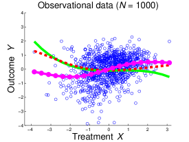
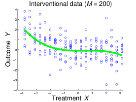
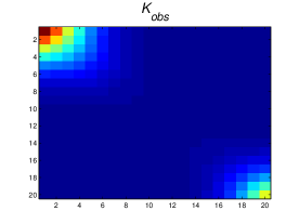
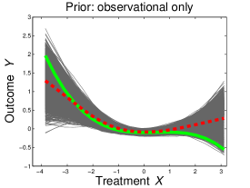
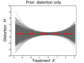
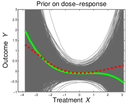
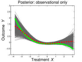
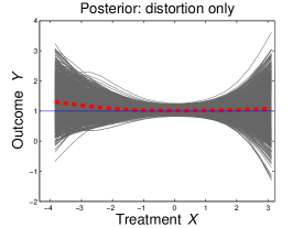
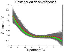
Figure 2 shows an example of inference obtained from synthetic data, generated according to the protocol of Section 4. In this example, the observational relationship between $X$ and $Y$ has the opposite association of the true causal one, but after adjusting for 15 of the 25 confounders that generated the data (10 confounders are randomly ignored to mimic imperfect prior knowledge), a reasonable initial estimate for $f(\mathcal{X})$ is obtained. The combination with interventional data results in a much better fit, but imperfections still exist at the strongest levels of treatment: the green curve drops at $x>2$ stronger than the expected posterior mean. This is due to having both a prior derived from observational data that got the wrong direction of the dose-response curve at $x>1.5$, and being unlucky at drawing several higher than expected values in the interventional regime for $x=3$. The model then shows its strength on capturing much of the structure of the true dose-response curve even under misspecified adjustments, but the example provides a warning that only so much can be done given unlucky draws from a small interventional dataset.

3.3 Inference, Stratified Learning and Active Learning

In our experiments, we infer posterior distributions by Gibbs sampling, alternating the sampling of latent variables $f(\mathcal{X})$, $a(\mathcal{X})$, $b(\mathcal{X})$ and hyperparameters $\lambda_{a}$, $\sigma_{a}$, $\lambda_{b}$, $\sigma_{b}$, $\sigma^{2}_{int}$, using slice sampling [16] for the hyperparameters. The meaning of the individual posterior distribution over $f_{obs}(\mathcal{X})$ might also be of interest. In principle, this quantity is potentially identifiable by considering a joint model for $(\mathcal{D}_{obs},\mathcal{D}_{int})$: in this case, $f_{obs}(\mathcal{X})$ learns the observational adjustment $\int g(x,\mathbf{z})p(\mathbf{z})\ d\mathbf{z}$. This suggests that the posterior distribution for $f_{obs}(\mathcal{X})$ will change little according to model (5), which is indeed observed in practice and illustrated by Figure 2. Learning the hyperparameters for $K_{obs}$ could be done jointly with the remaining hyperparameters, but the cost per iteration would be high due to the update of $K_{obs}$. The MCMC procedure for (5) is relatively inexpensive assuming that $|\mathcal{X}|$ is small. Learning the hyperparameters of $K_{obs}$ separately is a type of “modularization” of Bayesian inference [11].

As we mentioned in Section 2, it is sometimes desirable to learn dose-response curves conditioned on a few covariates $\mathbf{S}\subset\mathbf{Z}$ of interest. In particular, in this paper we will consider the case of straightforward stratification: given a set $\mathbf{S}$ of discrete covariates assuming instantiations $\mathbf{s}$, we have functions $f^{\mathbf{s}}(\mathcal{X})$ to be learned. Different estimation techniques can be used to borrow statistical strength across levels of $\mathbf{S}$, both for $f^{\mathbf{s}}(\mathcal{X})$ and $f^{\mathbf{s}}_{obs}(\mathcal{X})$. However, in our implementation, where we assume $|\mathbf{S}|$ is very small (a realistic case for many experimental designs), we construct independent priors for the different $f^{\mathbf{s}}_{obs}(\mathcal{X})$ with independent affine transformations.

Finally, in the Appendix we also consider simple active learning schemes [12], as suggested by the fact that prior information already provides different estimates of uncertainty across $\mathcal{X}$ (Figure 2), which is sometimes dramatically nonstationary.

4 Experiments

Assessing causal inference algorithms requires fitting and predicting data generated by expensive randomized trials. Since this is typically unavailable, we will use simulated data where the truth is known. We divide our experiments in two types: first, one where we generate random dose-response functions, which allows us to control the difficulty of the problem in different directions; second, one where we start from a real world dataset and generate “realistic” dose-response curves from which simulated data can be given as input to the method.

4.1 Synthetic Data Studies

We generate studies where the observational sample has $N=1000$ data points and $|\mathbf{Z}|=25$ confounders. Interventional data is generated at three different levels of sample size, $M=40$, $100$ and $200$ where the intervention space $\mathcal{X}$ is evenly distributed within the range shown by the observational data, with $|\mathcal{X}|=20$. Covariates $\mathbf{Z}$ are generated from a zero-mean, unit variance Gaussian with correlation of $0.5$ for all pairs. Treatment $X$ is generated by first sampling a function $f_{i}(z_{i})$ for every covariate from a Gaussian process, summing over $1\leq i\leq 25$ and adding Gaussian noise. Outcome $Y$ is generated by first sampling linear coefficients and one intercept to weight the contribution of confounders $\mathbf{Z}$, and then passing the linear combination through a quadratic function. The dose-response function of X on Y is generated as a polynomial, which is added to the contribution of $\mathbf{Z}$ and a Gaussian error. In this way, it is easy to obtain the dose-response function analytically.

Besides varying $M$, we vary the setup in three other aspects: first, the dose-response is either a quadratic or cubic polynomial; second, the contribution of $X$ is scaled to have its minimum and maximum value spam either $50\%$ or $80\%$ of the range of all other causes of $Y$, including the Gaussian noise (a spam of $50\%$ already generates functions of modest impact to the total variability of $Y$); third, the actual data given to the algorithm contains only 15 of the 25 confounders. We either discard 10 confounders uniformly at random (the Random setup), or remove the “top 10 strongest” confounders, as measured by how little confounding remains after adjusting for that single covariate alone (the Adversarial setup). In the interest of space, we provide a fully detailed description of the experimental setup in the Appendix. Code is also provided to regenerate our data and re-run all of these experiments.

Evaluation is done in two ways. First, by the normalized absolute difference between an estimate $\hat{f}(x)$ and the true $f(x)$, averaged over $\mathcal{X}$. The normalization is done by dividing the difference by the gap between the maximum and minimum true values of $f(\mathcal{X})$ within each simulated problem. The second measure is the log density of each true $f(x)$, averaged over $x\in\mathcal{X}$, according to the inferred posterior distribution approximated as a Gaussian distribution, with mean and variance estimated by MCMC. We compare our method against: I. a variation of it where $a$ and $b$ are fixed at $\mathbf{1}$ and $\mathbf{0}$, so the only randomness is in $f_{obs}$; II. instead of an affine transformation, we set $f(\mathcal{X})=f_{obs}(\mathcal{X})+r(\mathcal{X})$, where $r$ is given a generic squared exponential Gaussian process prior, which is fit by marginal maximum likelihood; III. Gaussian process regression with squared exponential kernel applied to the interventional data only and hyperparameters fitted by marginal likelihood. The idea is that competitors I and II provide sensitivity analysis of whether our more specialized prior is adding value. In particular, competitor II would be closer to the traditional priors used in computer-aided experimental design [2] (but for our specialized $K_{obs}$). Results are shown in Table 1, according to the two assessment criteria, using $\mathbb{E}$ for average absolute error, and $\mathcal{L}$ for average log-likelihood.

Table 1: For each experiment, we have either quadratic (Q) or cubic (C) ground truth, with a signal range of $50\%$ or $80\%$, and an interventional sample size of $M=40$, $100$ and $200$. $\mathbb{E}_{i}$ denotes the difference between competitor $i$ and our method regarding mean error, see text for a description of competitors. $\mathcal{L}_{i}$ denotes the difference between our method and competitor $i$ regarding log-likelihood (differences greater than 10 are ignored, see text). That is, positive values indicate our method is better according to the corresponding criterion. All results are averages over 50 independent simulations, italics indicate statistically significant differences by a two-tailed t-test at level $\alpha=0.05$.

	Q$50\%$ Random			Q$50\%$ Adv			Q$80\%$ Random			Q$80\%$ Adv
	40	100	200	40	100	200	40	100	200	40	100	200
$\mathbb{E}_{I}$	0.00	0.02	0.01	0.07	0.07	0.05	0.00	0.00	0.01	0.05	0.04	0.03
$\mathbb{E}_{II}$	0.05	0.02	0.01	0.04	0.00	0.00	0.04	0.03	0.02	0.04	0.02	0.00
$\mathbb{E}_{III}$	0.11	0.07	0.03	0.05	0.01	0.01	0.11	0.06	0.03	0.08	0.03	0.01
$\mathcal{L}_{I}$	2.33	2.31	2.18	7.16	6.68	6.23	0.62	0.53	0.45	2.16	1.79	1.50
$\mathcal{L}_{II}$	0.78	0.28	0.17	0.44	-0.17	-0.16	0.53	0.42	0.20	0.25	0.07	-0.09
$\mathcal{L}_{III}$	$>$ 10	$>$ 10	0.43	$>$ 10	$>$ 10	-0.06	0.74	0.44	0.36	0.33	-0.01	-0.10

	C$50\%$ Random			C$50\%$ Adv			C$80\%$ Random			C$80\%$ Adv
	40	100	200	40	100	200	40	100	200	40	100	200
$\mathbb{E}_{I}$	0.01	0.02	0.03	0.08	0.08	0.07	0.03	0.05	0.05	0.09	0.09	0.08
$\mathbb{E}_{II}$	0.05	0.03	0.02	0.05	0.02	0.01	0.05	0.03	0.02	0.07	0.03	0.02
$\mathbb{E}_{III}$	0.08	0.04	0.04	0.03	0.04	0.02	0.11	0.06	0.03	0.09	0.05	0.02
$\mathcal{L}_{I}$	$>$ 10	$>$ 10	$>$ 10	9.62	9.05	8.68	$>$ 10	$>$ 10	$>$ 10	$>$ 10	$>$ 10	$>$ 10
$\mathcal{L}_{II}$	3.49	0.83	0.41	4.45	0.43	-0.10	1.07	0.64	-0.04	0.96	0.30	0.14
$\mathcal{L}_{III}$	$>$ 10	$>$ 10	$>$ 10	$>$ 10	$>$ 10	$>$ 10	$>$ 10	0.79	0.03	0.45	0.18	-0.03

Our method demonstrated robustness to varying degrees of unmeasured confounding. Compared to Competitor I, the mean obtained without any further affine transformation already provides a competitive estimator of $f(\mathcal{X})$, but this suffers when unmeasured confounding is stronger (Adversarial setup). Moreover, uncertainty estimates given by Competitor I tend to be overconfident. Competitor II does not make use of our special covariance function for the correction, and tends to be particularly weak against our method in lower interventional sample sizes. In the same line, our advantage over Competitor III starts stronger at $M=40$ and diminishes as expected when $M$ increases. Competitor III is particularly bad at lower signal-to-noise ratio problems, where sometimes it is overly confident that $f(\mathcal{X})$ is zero everywhere (hence, we ignore large likelihood discrepancies in our evaluation). This suggests that in order to learn specialized curves for particular subpopulations, where $M$ will invariably be small, an end-to-end model for observational and interventional data might be essential.

4.2 Case Study

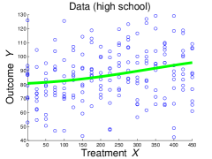
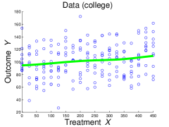
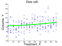
We consider an adaptation of the study analyzed by [8]. Targeted at premature infants with low birth weight, the Infant Health and Development Program (IHDP) was a study of the efficacy of “educational and family support services and pediatric follow-up offered during the first 3 years of life” [3]. The study originally randomized infants into those that received treatment and those that did not. The outcome variable was an IQ test applied when infants reached 3 years. Within those which received treatment, there was a range of number of days of treatment. That dose level was not randomized, and again we do not have ground truth for the dose-response curve. For our assessment, we fit a dose-response curve using Gaussian processes with Gaussian likelihood function and the back-door adjustment (3) on available covariates. We then use the model to generate independent synthetic “interventional data.” Measured covariates include birth weight, sex, whether the mother smoked during pregnancy, among other factors detailed by [8, 3]. The Appendix goes in detail about the preprocessing, including R/MATLAB scripts to generate the data. The observational sample contained 347 individuals (corresponding only to those which were eligible for treatment and had no missing outcome variable) and 21 covariates. This sample included 243 infants whose mother attended (some) high school but not college, and 104 with at least some college.

(a)	(b)	(c)

Figure 3: An illustration of a problem generated from a model fitted to real data. That is, we generated data from “interventions” simulated from a model that was fitted to an actual study on premature infant development [3], where the dose is the number of days that an infant is assigned to follow a development program and the outcome is an IQ test at age 3. (a) Posterior distribution for the stratum of infants whose mothers had up to some high school education, but no college. The red curve is the posterior mean of our method, and the blue curve the result of Gaussian process fit with interventional data only. (b) Posterior distributions for the infants whose mothers had (some) college education. (c) The combined strata.

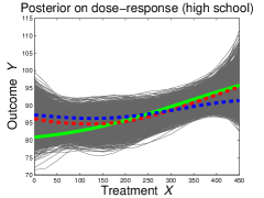
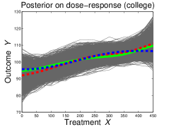
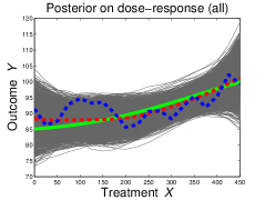
We generated 100 synthetic interventional datasets stratified by mother’s education, (some) high-school vs. (some) college. 19 treatment levels were pre-selected, amounting to 0 to 450 days with increments of 25 days. All variables were standardized to zero mean and unit standard deviation according to the observational distribution per stratum. Two representative simulated studies are shown in Figure 3, depicting dose-response curves which have modest evidence of non-linearity, and differ in range per stratum. On average, our method improved over the fitting of a Gaussian process with squared exponential covariance function that was given interventional data only. According to the average normalized absolute differences, the improvement was $0.06$, $0.07$ and $0.08$ for the high school, college and combined data, respectively (where error was reduced in $82\%$, $89\%$ and $91\%$ of the runs, respectively), each in which 10 interventional samples were simulated per treatment level per stratum.

5 Conclusion

We introduced a simple, principled way of combining observational and interventional measurements and assessed its accuracy and robustness. In particular, we emphasized robustness to model misspecification and we performed sensitivity analysis to assess the importance of each individual component of our prior, contrasted to off-the-shelf solutions that can be found in related domains [2].

We are aware that many practical problems remain. For instance, we have not discussed at all the important issue of sample selection bias, where volunteers for an interventional study might not come from the same $p(\mathbf{Z})$ distribution as in the observational study. Worse, neither the observational nor the interventional data might come from the population in which we want to enforce a policy learned from the combined data. While these essential issues were ignored, our method can in principle be combined with ways of assessing and correcting for sample selection bias [1]. Moreover, if unmeasured confounding is too strong, one cannot expect to do well. Methods for sensitivity analysis of confounding assumptions [14] can be integrated with our framework. A more thorough analysis of active learning using our approach, particularly in the light of possible model misspecification, is needed as our results in the Appendix only superficially covers this aspect.

Acknowledgments

The author would like to thank Jennifer Hill for helping with the IHDP data, and Robert Gramacy for several useful discussions.

Appendix

In this Appendix, we discuss: i. a detailed explanation of our synthetic data generation protocol; ii. a detailed explanation of our preprocessing of the Infant Health and Development Program dataset; iii. an illustration of active learning using our approach; iv. an illustrative comparison of our method against existing methods for deep Gaussian processes in the literature.

A Synthetic Data Generator

We generate data from a multivariate distribution where $X$ is the treatment, $Y$ is the outcome, and $\mathbf{Z}$ are covariates that cause $X$ and $Y$. The model for the covariates is

$$\mathbf{Z}\sim\mathcal{N}(\mathbf{0},\Sigma_{\mathbf{Z}}),$$

where $\Sigma_{\mathbf{Z}}$ is a correlation matrix with every off-diagonal entry equal to $0.5$.

The model for $\mathbf{X}$ given $\mathbf{Z}$ is

$$X=\sum_{i=1}^{p}f_{x_{i}}(z_{i})+e_{X},$$

where $p=|\mathbf{Z}|$ and $e_{X}\sim N(0,\sigma_{x}^{2})$. Each function $f_{x_{i}}(\cdot)$ is first sampled at the realized values of $Z_{i}$ from a zero-mean Gaussian process prior with covariance function $k(z_{i},z_{i}^{\prime})\equiv\exp(-(z_{i}-z_{i}^{\prime})^{2}/4)$, then divided by $\sqrt{p}$ so that the variance of the function generation process does not grow with $p$. We then calculate the empirical variance $v_{f_{x}}$ of $\sum_{i}f_{x_{i}}(Z_{i})$ in the sample generated, and set $\sigma_{x}^{2}=b\times v_{f_{x}}$, where $b\sim\mathcal{U}(0.2,0.4)$, the uniform distribution in the interval $[0.2,0.4]$. In this way, causes of $X$ that are not causes of $Y$ (that is, $e_{X}$) contribute to the variance of $X$ with approximately $20\%$ to $40\%$ of the variance contributed by the common causes.

The next step is to generate

$$\theta_{i}\sim\mathcal{N}\left(0,\frac{1}{p+1}\right),$$

for $0\leq i\leq p$, and

$$\beta_{i}\propto\mathcal{N}(0,1)I(|\beta_{i}|>0.2),$$

$i\in\{0,1,2\}$ and $I(\cdot)$ the indicator function. That is, each $\beta_{i}$ comes from a standard Gaussian restricted to the space $|\beta_{i}|>0.2$. We then define

$$\begin{array}[]{rcl}Z_{y}&\equiv&\theta_{0}+\theta_{1:p}^{\top}\mathbf{Z}\\ f_{yz}&\equiv&\beta_{2}Z_{y}^{2}+\beta_{1}Z_{y}+\beta_{0}\\ f_{yze}&\equiv&f_{yz}+e_{Y}\\ e_{Y}&\sim&\mathcal{N}(0,\sigma^{2}_{y}).\\ \end{array}$$

Quantity $f_{yze}$ is the contribution of “all other causes” of $Y$ but $X$. Analogously to $\sigma_{x}^{2}$, we set $\sigma^{2}_{y}=b^{\prime}\times v_{f_{yz}}$, where $b^{\prime}\sim\mathcal{U}(0.2,0.4)$ and $v_{f_{yz}}$ is the empirical variance of the sampled values of $f_{yz}$. What is left is the contribution of $X$ according to

$$Y=f_{yx}(X)+f_{yze},$$

in a way we can control (up to some point) how much $X$ contributes to the variability of $Y$. Function $f_{yx}(\cdot)$ is set to be a polynomial of degree $d$. In our experiments, we set $d=2$ and $d=3$.

Let $\alpha$ be a number between 0 and $0.5$. Let $R_{\alpha}$ and $R_{1-\alpha}$ be the corresponding empirical quantiles of $f_{yze}$. Define $R\equiv R_{1-\alpha}-R_{\alpha}$. In our experiments, we choose either $\alpha=0.1$ or $\alpha=0.25$. We constraint our $f_{yze}$ to be within a range of length $R$ as follows. For any realization $x$ of $X$, define $\hat{x}$ as the standardization of $x$ according to the empirical mean and variance of the sampled values of $X$. That is, given the empirical mean $\hat{m}$ of the sampled values of $X$ and the empirical variance $\hat{v}$, $\hat{x}\equiv(x-\hat{m})/\sqrt{\hat{v}}$. Both $\hat{m}$ and $\hat{v}$ become extra parameters of $f_{yx}(\cdot)$. Given a degree $d$, we set

$$\begin{array}[]{rcl}\lambda_{i}^{\prime}&\propto&\mathcal{N}(0,1)I(|\lambda_{i}|>0.2)\\ f_{yx}^{\prime}(x)&\equiv&\displaystyle\sum_{i=0}^{d}\lambda_{i}^{\prime}\hat{x}^{i},\\ R^{\prime}&\equiv&\displaystyle\max f_{yx}^{\prime}(\hat{x})-\min f_{yx}^{\prime}(\hat{x})\\ \lambda_{i}&\equiv&\displaystyle\alpha_{i}^{\prime}\times\frac{R}{R^{\prime}}\\ f_{yx}(x)&\equiv&\displaystyle\sum_{i=0}^{d}\lambda_{i}\hat{x}^{i}.\end{array}$$

In the third line of the above, the maximum and minimum operations are taken over the empirical samples of $X$. The end result is a function that first linearly transforms $X$ to a more standard scale and location, then passes it to a polynomial function with a range is approximately of the same length as the difference between the $1-\alpha$ and $\alpha$ quantiles of the realizations of $f_{yze}$. Setting $\alpha$ to values close to $0.5$ would make the signal due to $X$ to be mostly constant, its variability almost undetectable compared to the variability of the other causes of $Y$. Finally, we reject this model and redo the model generating process if the absolute value of the empirical rank correlation between the samples of $X$ and $f_{yz}$ is less than 0.2, so that a minimal degree of confounding is enforced.

Notice that the motivation for setting $\mathbf{Z}\sim\mathcal{N}(\mathbf{0},\Sigma_{\mathbf{Z}})$, and $f_{yz}(\mathbf{Z})$ to a quadratic function, is to allow us to analytically calculate $\mathbb{E}[f_{yz}(\mathbf{Z})]$. This is important, since

$$\mathbb{E}[Y\ |\ do(X=x)]=f_{yx}(x)+\mathbb{E}[f_{yz}(\mathbf{Z})],$$

the value of which is necessary for a precise calculation of the estimation error.

We provide MATLAB code to reconstruct the experiments at http://www.homepages.ucl.ac.uk/~ucgtrbd/code/obsint. This is done via the function generate_problems.m, which can also make use of a file that provides the seed to reconstruct the synthetic models and data exactly.

To complement the results in the main text, Table 2 shows further comparisons. Method IV is the one obtained by just fitting the observational data for treatment and outcome, assuming no confounding (that is, no back-door adjustment is done). It provides a sense of the difficulty of the generated problems. Method V is yet another sensitivity analysis, now for the role of $a$. This is done by effectively dropping $a$ from the mapping between $f_{obs}$ and $f$ (that is, the generation of $f$ is defined as $f(\mathcal{X})\equiv f_{obs}(\mathcal{X})+b(\mathcal{X})$). It differs from Method III in the main text by giving $b$ a non-stationary covariance function derived from $\mathcal{D}_{obs}$, as opposed to the off-the-shelf squared exponential used by Method III. It is clear that although the $a$ component does not seem to help (or hurt) the decrease of the absolute error, it makes a significant difference in terms of modeling the posterior uncertainty. Differences are more prominent under the Adversarial regime, which can be partially explained by the heavy-tailed, non-Gaussian nature of the product $a\odot f_{obs}$. We emphasize that our measure $\mathcal{L}_{V}$ is per point $x\in\mathcal{X}$, and that even a difference of $0.05$ in average log-likelihood means a ratio of densities of $2.7$ in the original scale, for $|\mathcal{X}|=20$, and a ratio of approximately $20,000$ for a difference of $0.50$.

Table 2: A table analogous to the one found in the main text, Section 4. Here, method IV is just the dose-response obtained by fitting the observational data only without any back-door adjustment. Method V is the method where we set $a\equiv\mathbf{1}$, inferring $b$ only.

	Q$50\%$ Random			Q$50\%$ Adv			Q$80\%$ Random			Q$80\%$ Adv
	40	100	200	40	100	200	40	100	200	40	100	200
$\mathbb{E}_{IV}$	0.41	0.45	0.47	0.36	0.41	0.44	0.30	0.34	0.37	0.28	0.33	0.36
$\mathbb{E}_{V}$	-0.01	0.00	0.00	0.01	0.01	0.01	0.00	0.00	0.00	0.00	0.01	0.01
$\mathcal{L}_{V}$	-0.01	0.04	0.08	0.31	0.47	0.55	0.01	0.07	0.08	0.21	0.32	0.37

	C$50\%$ Random			C$50\%$ Adv			C$80\%$ Random			C$80\%$ Adv
	40	100	200	40	100	200	40	100	200	40	100	200
$\mathbb{E}_{IV}$	0.30	0.32	0.35	0.27	0.30	0.33	0.30	0.34	0.37	0.28	0.33	0.36
$\mathbb{E}_{V}$	0.00	0.00	0.00	0.01	0.00	0.00	0.00	0.00	0.01	0.00	0.01	0.01
$\mathcal{L}_{V}$	-0.02	0.01	0.04	0.19	0.25	0.36	0.06	0.14	0.30	0.22	0.40	0.50

B Preprocessing of the Infant Health and Development Program Data

The original Infant Health and Development Program (IHDP) data can be downloaded from http://www.icpsr.umich.edu/icpsrweb/HMCA/studies/9795. We start instead from the preprocessed version done by [8] and available at http://www.tandfonline.com/doi/suppl/10.1198/jcgs.2010.08162. This data contains 985 individuals, or which 377 were given treatment. 30 individuals had missing outcome data. We discarded them to obtain a final sample size of 347. We applied further preprocessing to this data, to remove variables which we believed would be less relevant to our simulation (for instance, the home site of the family at the start of the intervention). Some variables were binarized, as we were concerned about the sample size. This includes some originally discrete, non-binary, variables, such as race. A detailed R script that loads the original file provided by [8] and performs the further processing is provided with our code as (process_ihdp.R).

(a)	(b)	(c)

Figure 4: Example of synthetic data sampled from the three models (stratified by mother’s education, and then combined). The amount of variability around each response is similar to the one found around the observational regression curve. Curve represents the synthetic dose-response curve fitted to each scenario based on an observational sample of size $347$.

This resulted in a dataset with 21 columns. We fit a nonparametric model for the regression function $g(x,\mathbf{z})$ using a Gaussian process prior and Gaussian likelihood. The prior is the same as all other experiments, a Matérn $\nicefrac{{3}}{{2}}$ covariance function with automatic relevance determination priors [13]. We fit all hyperparameters by marginal maximum likelihood using the GPML package for MATLAB. The range of days of treatment in the treated IHDP subgroup varied from 0 to 468. We defined our set $\mathcal{X}$ of interventional levels at $0,25,50,\dots,450$.

To build a simulator for outcome variable $Y$, IQ score at age 3 (standardized by centering and scaling it according the the empirical mean and standard deviation of the observational data), we build a mean function $f(x)$ and error variance $\sigma_{f}^{2}$ from the fitted response function evaluated at the empirical observational distribution,

$$f(x)\equiv\frac{1}{347}\sum_{i=1}^{347}\hat{g}(x,\mathbf{z}^{(i)}),x\in\mathcal{X}.$$

Less straightforward is deciding on a realistic choice of $\sigma_{f}^{2}$. First, it should be pointed out that as implied by the fitted observational model as ground truth,

$$Y\ |\ do(x),\mathbf{z}\sim\mathcal{N}(\hat{g}(x,\mathbf{z}),\hat{\sigma}^{2}_{Y}),$$

where $\hat{\sigma}^{2}_{Y}$ is given by GPML, that $Y\ |\ do(x)$ will in general have heteroscedastic variance (if $\hat{g}(x,\mathbf{z})$ is not additive in $X$), or even be non-Gaussian distributed. To deal with that, we calculate the empirical variance of $\{\hat{g}(x,\mathbf{z}^{(1)}),\dots,\hat{g}(x,\mathbf{z}^{(347)})\}$ for each $x\in\mathcal{X}$, and set $\sigma_{f}^{2}$ to be the average of these quantities plus the error variance of the regression of $Y$ on $X$ and $\mathbf{Z}$. Normality is used as a convenient approximation for the resulting model $Y\ |\ do(x)$. Heteroscedastic regression can be adopted by our framework without any conceptual changes, but we ignore it for convenience of presentation.

C Active Learning Illustration

The probabilistic formulation of our dose-response model leads to Bayesian active learning schemes where observational data $\mathcal{D}_{obs}$ is fixed and new measurements are continuously added to interventional dataset $\mathcal{D}_{int}$. In this Section, we provide an illustration on how to use our model with the simplest design scheme: the “D-optimal” design where the next dose level $x$ to be picked is the one corresponding to target $f(x)$ of highest entropy. A classical review of the motivations and shortcomings of several designs from a Bayesian perspective is given by [12].

To approximate the entropy of a given $f(x)$, we merely compute its estimated variance from the current MCMC samples as we observe that in the posterior the marginal distributions of each $f(x)$ are not too dissimilar from Gaussians, or at least can be ranked based on variances alone. Use of the variance can be formally justified by standard second-order approximations [12] even if we still rely on MCMC samples.

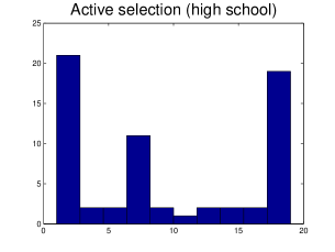
We applied this idea to our IHDP problem, where we initialize the model by sampling one outcome for each dose level $x\in\mathcal{X}$. We then are given a budget of $5\times|\mathcal{X}|=95$ trials to spend. For every new dose level selected, we “run the intervention” using our simulated model, and collect a new data point. We update the distribution of the latent variables at every new point collected, but to save time we update the distribution of the hyperparameters only after 5 new points have been collected. The budget of $95$ points is shared across the two strata. In our provided MATLAB code, function dose_response_learning_stratified.m implements this scheme.

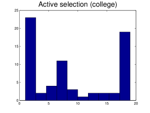
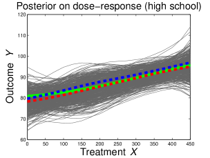
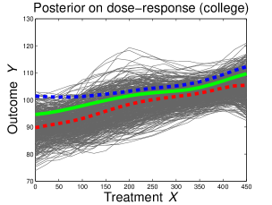
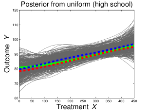
In Figure 5, we show how treatments were allocated to each stratum, and how they were distributed. As expected, most of the doses were given at the endpoints of $\mathcal{X}$. Stratum “high school” was allocated $31$ of the $95$ (simulated) trials, with the remaining $64$ given to the “college” stratum. We compare it against the policy of allocating an equal number ($6$) of trials to each of the $19$ levels of $\mathcal{X}$. Figure 6 illustrates the posterior distributions for the samplers given one actively selected set and one uniformly selected set. While the differences are not major, it is clear that the active scheme does better or at least as well even in regions were no more than two datapoints have been collected, with a clear advantage in regions where the prior was not able to capture the true curve (lower levels of stratum “high school”).

Figure 5: Histogram of the allocation of $114$ experiments (initial 19 followed by adaptively selected 95 further trials) in two different conditions according to our simple active learning criteria.

Figure 6: Corresponding models learned from this data. The red curve corresponds to the expected dose-response according to the collected sample, while the blue curve is the result of our procedure with a given set of $133$ uniformly sampled at our $\mathcal{X}$ grid of 19 dose levels. The top row illustrates samples from the posterior learned from the active selection, the bottom row are samples from the posterior learned from the uniform selection. In general, there is a slight advantage for the active selection at this sample size, as the posterior typically allocates higher probability to the true curve.

Figure 7: A comparison of results for the IHDP data using a more standard (non-factorized) deep Gaussian process prior against our factorized prior. For the non-factorized model, Hamiltonian MCMC was used. Each plot show 200 sampled dose-response curves. In the factorized case, these correspond to thinning a run of 2000 iterations by skipping 10 samples from every sample held.

D A Note on Generic Deep Gaussian Processes

The transformation given by $a$ and $b$ is not identifiable: like a deep Gaussian process prior [5], its usefulness comes from providing an adequate prior distribution for $f$ that we evaluated at length through a series of comparisons and sensitivity analyzes.

In any case, this raises the question of directly adopting the generic transformation of $f_{obs}(\mathcal{X})$,

$$f(x)=u(f_{obs}(x)),x\in\mathcal{X},$$

where $u(\mathcal{X})$ is a function that is given a Gaussian process prior. One appropriate choice of mean for this process is the identity function, $\mu_{u}(f_{obs}(x))=f_{obs}(x)$, with the covariance matrix $K_{u}$ constructed from smooth covariance functions, as we want to bias this prior toward the (unknown) observational curve $f_{obs}(\mathcal{X})$.

It is not clear, however, why this generic construction would have advantages over our pointwise affine prior. The original motivation for deep learning is to combine signals from a high-dimensional space, and here our treatment is a scalar dosage. Our goal in this section is just to provide a simple illustration that, for a dose-response curve where the signal is just a scalar, there is no obvious reason to use more complicated models.

Sampling $f_{obs}(\cdot)$ in this “deep” setup is difficult due to its appearance on $K_{u}$. We illustrate the advantages of our pointwise affine prior with a simple experiment, once again based on the IHDP data. We define $K_{u}$ with a squared exponential covariance function,

$$k_{u}(f_{obs}(x),f_{obs}(x^{\prime}))\equiv\lambda_{u}\times\exp\left(-\frac{1}{2}\frac{(f_{obs}(x)-f_{obs}(x^{\prime})^{2}}{\sigma_{u}}\right)+\delta(f_{obs}(x)-f_{obs}(x^{\prime}))10^{-5}$$

with priors $\log(\lambda_{u})\sim\mathcal{N}(0,0.5)$ and $\log(\sigma_{u})\sim\mathcal{N}(0,0.1)$. Moreover, we rescale the covariance matrix of $f_{obs}(\mathcal{X})$ so that the largest entry of its diagonal is now 1. This is to give the standard deep GP an extra help, as exploring the posterior of $f_{obs}(\cdot)$ and the hyperparameters would be even harder with a more concentrated prior. We also enforce no parameter sharing of any kind among the different strata. In what follows, we do not claim that this prior is optimal for learning the dose-response curve, but as a convenient way of facilitating sampling for this model.

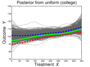
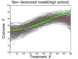
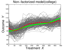
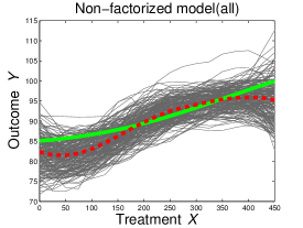
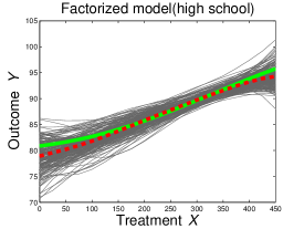
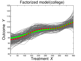
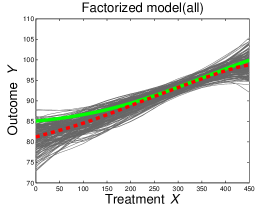
In Figure 7, we show posterior samples for the standard Gaussian process prior using the default Hamiltonian MCMC (HMC) methods implemented in Stan [4]. The dataset given contains $10$ points per dose level of $\mathcal{X}$ in each of the three scenarios ($190$ per study, in total). Due to the high cost of performing sampling even in these modest datasets, we run HMC only for $220$ iterations, discarding the first $20$ iterations as burn-in. We run the off-the-shelf Gibbs with the slice sampling algorithm for our affine model. In Figure 7, we show the corresponding output obtained by running it for $2200$ iterations, discarding the first $200$, and then uniformly thinning the remaining $2000$ iterations to obtain $200$ samples.

It is clear that in Figure 7 that the affine prior performs substantially better. However, we do not want to make overgeneralized claims of inferential superiority, but to merely illustrate that we see no evidence that a standard deep Gaussian process prior would present any advantage. This is even more evident from the computational cost of both procedures. The HMC execution, even in the highly optimized Stan code, took approximately $1200$ seconds in a 5-year old Xeon workstation, while inference with the factorized prior took two orders of magnitude less, $54$ seconds. While powerful approximation algorithms can be applied to standard deep Gaussian processes [5], we recommend avoiding them, as in causal inference we are interested in parameter learning instead of merely predictive performance and the more precise calculation of credible intervals provided by MCMC is preferred to a variational approximation that will underestimate uncertainty.

References

- [1] E. Bareinboim and J. Pearl. Causal inference from Big Data: Theoretical foundations and the data-fusion problem. Proceedings of the National Academy of Sciences, in press, 2016.
- [2] M. J. Bayarri, J. O. Berger, R. Paulo, J. Sacks, J. A. Cafeo, J. Cavendish, C.-H. Lin, and J. Tu. A framework for validation of computer models. Technometrics, 49:138–154, 2007.
- [3] J. Brooks-Gunn, F. Liaw, and P. Klebanov. Effects of early intervention on cognitive function of low birth weight preterm infants. Journal of Pediatrics, 120:350–359, 1991.
- [4] B. Carpenter, A. Gelman, M. Hoffman, D. Lee, B. Goodrich, M. Betancourt, M. A. Brubaker, J. Guo, P. Li, and A. Riddell. Stan: A probabilistic programming language. Journal of Statistical Software, in press, 2016.
- [5] A. Damianou and N. D. Lawrence. Deep Gaussian processes. Proceedings of the Sixteenth International Conference on Artificial Intelligence and Statistics (AISTATS), pages 207–215, 2013.
- [6] J. Ernest and P. Bühlmann. Marginal integration for nonparametric causal inference. Electronic Journal of Statistics, 9:3155–3194, 2015.
- [7] R. Gramacy and H. K. Lee. Bayesian treed Gaussian process models with an application to computer modeling. Journal of the American Statistical Association, 103:1119–1130, 2008.
- [8] J. Hill. Bayesian nonparametric modeling for causal inference. Journal of Computational and Graphical Statistics, 20:217–240, 2011.
- [9] J. Hill and Y.-S. Su. Assessing lack of common support in causal inference using Bayesian nonparametrics: Implications for evaluating the effect of breastfeeding on children’s cognitive outcomes. The Annals of Applied Statistics, 7:1386–1420, 2013.
- [10] A. Hyttinen, F. Eberhardt, and P. O. Hoyer. Experiment selection for causal discovery. Journal of Machine Learning Research, 14:3041–3071, 2013.
- [11] F. Liu, M. J. Bayarri, and J. O. Berger. Modularization in Bayesian analysis, with emphasis on analysis of computer models. Bayesian Analysis, 4:119–150, 2009.
- [12] D. J. C. MacKay. Information-based objective functions for active data selection. Neural Computation, 4:590–604, 1992.
- [13] D. J. C. MacKay. Bayesian non-linear modelling for the prediction competition. ASHRAE Transactions, 100:1053–1062, 1994.
- [14] L. C. McCandless, P. Gustafson, and A. R. Levy. Bayesian sensitivity analysis for unmeasured confounding in observational studies. Statistics in Medicine, 26:2331–2347, 2007.
- [15] S. L. Morgan and C. Winship. Counterfactuals and Causal Inference: Methods and Principles for Social Research. Cambridge University Press, 2014.
- [16] R. Neal. Slice sampling. The Annals of Statistics, 31:705–767, 2003.
- [17] J. Pearl. Causality: Models, Reasoning and Inference. Cambridge University Press, 2000.
- [18] C. Rasmussen and C. Williams. Gaussian Processes for Machine Learning. MIT Press, 2006.
- [19] J. Robins, M. Sued, Q. Lei-Gomez, and A. Rotnitzky. Comment: Performance of double-robust estimators when ”inverse probability” weights are highly variable. Statistical Science, 22:544–559, 2007.
- [20] P. Spirtes, C. Glymour, and R. Scheines. Causation, Prediction and Search. Cambridge University Press, 2000.
- [21] T. VanderWeele and I. Shpitser. A new criterion for confounder selection. Biometrics, 64:1406–1413, 2011.