Anisotropy of the monomer random walk in a polymer melt: local-order and connectivity effects

Abstract

The random walk of a bonded monomer in a polymer melt is anisotropic due to local order and bond connectivity. We investigate both effects by molecular-dynamics simulations on melts of fully-flexible linear chains ranging from dimers ($M=2$) up to entangled polymers ($M=200$). The corresponding atomic liquid is also considered as reference system. To disentangle the influence of the local geometry and the bond arrangements, and reveal their interplay, we define suitable measures of the anisotropy emphasising either the former or the latter aspect. Connectivity anisotropy, as measured by the correlation between the initial bond orientation and the direction of the subsequent monomer displacement, shows a slight enhancement due to the local order at times shorter than the structural relaxation time. At intermediate times - when the monomer displacement is comparable to the bond length - a pronounced peak and then decays slowly as $t^{-1/2}$, becoming negligible when the displacements is as large as about five bond lengths, i.e. about four monomer diameters or three Kuhn lengths. Local-geometry anisotropy, as measured by the correlation between the initial orientation of a characteristic axis of the Voronoi cell and the subsequent monomer dynamics, is affected at shorter times than the structural relaxation time by the cage shape with antagonistic disturbance by the connectivity. Differently, at longer times, the connectivity favours the persistence of the local-geometry anisotropy which vanishes when the monomer displacement exceeds the bond length. Our results strongly suggest that the sole consideration of the local order is not enough to understand the microscopic origin of the rattling amplitude of the trapped monomer in the cage of the neighbours.

1 Introduction

The relation between the structure and the dynamics is a key problem in liquid-state [1, 2, 3] and polymer [4, 5] physics. In particular, in a liquid of particles the random walk of the constituents is affected at short times (or length scales comparable to the particle diameter) by the local order and the displacement is anisotropic, differing by the one of a brownian particle in an homogeneous liquid [6, 7, 8]. In a polymer melt, the anisotropy of the bonded-monomer displacement is also contributed by the bond connectivity [9, 10, 11]. While the local-order anisotropy (LOA) is expected to be stronger at shorter times, the connectivity anisotropy (COA) is anticipated to be important at both short and long times, since it involves the connected particles on different length scales [9, 10, 11]. The interplay between the connectivity and the local order is, at least in part, antagonistic [12]. In fact, the connectivity introduces a length scale, the bond length, which perturbs the local order with characteristic length scale given by the particle size, in general not commensurate with the bond length.

Our interest in the relation between particle displacement and local ordering is motivated by a number of arguments. The main motivation is the pursuit of the microscopic origin of the universal correlation between the mean square amplitude of the cage rattling (related to the Debye-Waller factor) and the relaxation and transport, as found in simulations of polymers [13, 14, 15], binary atomic mixtures [14, 16], colloidal gels [17] and antiplasticized polymers [18, 19], and supported by the experimental data concerning several glassformers in a wide fragility range ($20\leq m\leq 191$) [13, 20, 21, 16, 22]. From this respect, the local structure due to the first neighbours was recently found to correlate poorly with the rattling amplitude in the cage of the closest neighbours, and the structural relaxation, in liquids of linear trimers [23, 24] and atomic mixtures [23]. On the other hand, extended modes ranging up to about the fourth shell do correlate with the rattling amplitude in the cage and the structural relaxation [25, 26]. These two complementary findings are fully consistent with Berthier and Jack who concluded that the influence of structure on dynamics is weak on short length scale and becomes much stronger on long length scale [27]. On a more general grounds, several approaches suggest that structural aspects matter in the dynamics of glassforming systems. This includes the Adam-Gibbs derivation of the structural relaxation [28, 29] - built on the thermodynamic notion of the configurational entropy [30] -, the mode- coupling theory [2] and extensions [31], the random first-order transition theory [32], the frustration-based approach [33], as well as the so-called elastic models [34, 35, 36, 37, 38, 39, 40, 41, 42, 43, 19, 44, 45, 46, 47] in that the modulus is set by the arrangement of the particles in mechanical equilibrium and their mutual interactions [34, 44]. It was concluded that the proper inclusion of many-body static correlations in theories of the glass transition appears crucial for the description of the dynamics of fragile glass formers [48]. The search of a link between structural ordering and slow dynamics motivated several studies in liquids [49, 50, 51, 52, 53] colloids [54, 55, 56] and polymeric systems [54, 57, 58, 59, 60, 61, 62].

Here, we present a detailed study of both LOA and COA anisotropies of the bonded monomers by molecular-dynamics (MD) simulation of a polymeric melt of linear chains and an atomic liquid (as reference system in one particular state). As to the polymer melt, particular attention is devoted to temperature and the chain length which is changed from oligomers (trimers, $M=3$) up to entangled systems ($M=200$).

LOA is characterized by the correlation between the initial shape of the cage of the closest neighbours and the direction of the subsequent monomer displacement. We are inspired by a seminal work by Rahman in an atomic liquid [63], studying the directional correlations between the particle dynamics of the trapped particle in the cage and the position of the centroid C of the vertices of the associated Voronoi polyhedron (VP). The interest relies on the fact that the VP vertices are located close to the voids between the particles and thus mark the weak spots of the cage. It has been shown in simulations of atomic liquids [63] and experiments on granular matter [64] that the particle initially moves towards the centroid, so that cage rattling and VP geometry are correlated at very short times. We are not aware of extensions to molecular liquids where COA is present.

COA is quantified by the correlation between the initial bond orientation and the direction of the monomer displacement.

The paper is organized as follows. In Sec. 2 the molecular model and the MD algorithms are presented. The results are discussed in Sec. 3 and the conclusions are summarized in Sec.4.

2 Methods

A coarse-grained model of a melt of $N_{c}$ linear fully-flexible polymer chains with $M$ monomers per chain is considered. Full flexibility is ensured by the absence of both torsional or bending potentials hindering the bond orientations. We set $M=2,3,5,10,15,30,100,200$. Entanglements are expected for lengths exceeding $M_{e}$ with $M_{e}$ estimated, according to different methods, as $\simeq 70$ [65] $\simeq 74$ [66] and $\simeq 80$ [67]. Non-bonded monomers at a distance $r$ interact via a truncated Lennard-Jones (LJ) potential $U_{LJ}(r)=\varepsilon\left[\left(\sigma^{*}/r\right)^{12}-2\left(\sigma^{*}/r\right)^{6}\right]+U_{cut}$ for $r<r_{c}=2.5\,\sigma$ and zero otherwise, where $\sigma^{*}=\sqrt[6]{2}\,\sigma$ is the position of the potential minimum with depth $\varepsilon$. The value of the constant $U_{cut}$ is chosen to ensure that $U_{LJ}(r)$ is continuous at $r=r_{c}$. The bonded monomers interact by a potential which is the sum of the LJ potential and the FENE (finitely extended nonlinear elastic) potential $U^{FENE}(r)=-{1/2}\;kR_{0}^{2}\;\ln\left(1-r^{2}/R_{0}^{2}\right)$ where $k$ measures the magnitude of the interaction and $R_{0}$ is the maximum elongation distance [5, 24]. The parameters $k$ and $R_{0}$ have been set to $30\,\varepsilon/\sigma^{2}$ and $1.5\,\sigma$ respectively [68]. The resulting bond length is $b=0.97\sigma$ within a few percent. All quantities are in reduced units: length in units of $\sigma$, temperature in units of $\varepsilon/k_{B}$ (with $k_{B}$ the Boltzmann constant) and time $\tau_{MD}$ in units of $\sigma\sqrt{m/\varepsilon}$ where $m$ is the monomer mass. We set $m=k_{B}=1$. We investigate states with number density $\rho=1.086$, temperature $T=1$ and $(N_{c},M)$ pairs: (1000, 2), (667, 3), (400, 5), (200, 10), (134, 15), (67, 30), (20, 100) and (60, 200). We also investigate states with $T=0.9,0.8,0.7,0.63,0.6$ for the pair (667, 3). In order to investigate the role of the connectivity we simulate an atomic Lennard-Jones liquid of $8000$ atoms at density $\rho=1.086$ and temperature $T=1.5$ and a molecular system at the same density and temperature with pair (2667, 3). Periodic boundary conditions are used. $NVT$ ensemble (constant number of particles, volume and temperature) has been used for equilibration runs, while $NVE$ ensemble (constant number of particles, volume and energy) has been used for production runs of a given state point with time step $3\cdot 10^{-3}$ [69]. The samples were equilibrated in lapses of time as long as, at least, three times the longest relaxation time, i.e. the average reorientation time of the chain $\tau_{r}$. The simulations are carried out using LAMMPS molecular dynamics software (http://lammps.sandia.gov) [70].

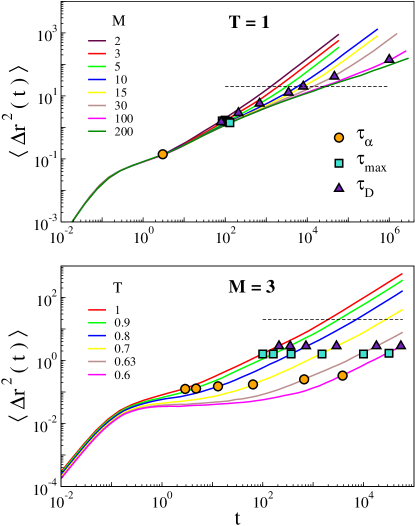
Figure 1: Monomer MSD for different chain lengths at $T=1$ (top) and for trimers at different temperatures (bottom). The orange circles mark the structural relaxation time $\tau_{\alpha}$. The turquoise squares mark the time $\tau_{max}$ where the COA function $\widehat{C}(t)$, Eq.4, is maximum (see Fig.4). The violet triangles mark the onset time $\tau_{D}$ of the diffusion regime defined by Eq.1. When MSD exceeds the threshold, $\sim 20$, signalled by the dashed line, $\widehat{C}(t)$ drops below $0.1$. The threshold is virtually independent of the chain length and corresponds to about five bond lengths, i.e. about four monomer diameters.

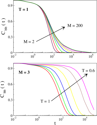
Figure 2: Bond-bond correlation function $C_{bb}(t)$, Eq.2, for different chain lengths at $T=1$ (top) and for trimers at different temperatures (bottom). Color codes as in Fig.1. At long times $C_{bb}(t)\simeq\exp[-(t/\tau^{\prime})^{\beta}]$ [71]. The stretching parameter ranges between $\beta_{M=200}\simeq 0.15$ and $\beta_{M=2}\simeq 0.9$.

3 Results and discussion

3.1 General aspects: monomer displacement and bond reorientation

Fig.1 shows an overview of the dependence of the monomer mean-square-displacement (MSD) on the chain length (top) and temperature (bottom). At short times ($t\sim 0.1$), after the ballistic regime, the repeated collisions with the surroundings slow down the monomers and temporarily traps them in the cage formed by the first neighbours. The monomers escape from the cage on average within the time $\tau_{\alpha}$ (orange circles of Fig.1). We define, as in previous works [13, 14, 15, 16, 17, 20, 21, 23, 25, 44, 46, 71, 72], the structural relaxation time by the equation $F_{s}(q_{max},\tau_{\alpha})=\phi$ with $\phi=e^{-1}$ where $q_{max}$ is the maximum of the static structure factor and $F_{s}$ is the self-part of the intermediate scattering function [1]. It is worth noting that our polymer model complies with the temperature-time superposition principle, resulting in a constant (and moderate) stretching of $F_{s}(q_{max},t)$ [13]. Then, even if other definitions of $\tau_{\alpha}$ are possible, e.g. by setting $\phi=0.1$ [15], these alternatives differ from the present one of a constant factor of $\sim 3$, insignificant to the purposes of the present paper. In the present polymer model $\tau_{\alpha}$ is little dependent on $M$ since the chains are fully flexible [15].

For times longer than $\tau_{\alpha}$ the polymer connectivity limits the monomer displacement and a series of different regimes are observed, all being characterized by subdiffusive motion, i.e. MSD $\propto t^{\gamma}$ with $\gamma<1$ [9, 10, 11, 73, 74]. The subdiffusive regimes are not of interest in the present paper. Their detailed description is found in textbooks [9, 10, 11] and will be not repeated here for conciseness. Subdiffusive motion ends when the monomer moves a distance of the order of the chain size, the end-end mean square distance of the chain $R_{ee}^{2}$, and the diffusive regime is entered ($\gamma=1$) [9, 10, 11]. For the present polymer model one has $R_{ee}^{2}=C_{\infty}(M-1)\;b^{2}$ with characteristic ratio $C_{\infty}\simeq 1.51$, in agreement with previous work [72].

Let us define the time $\tau_{D}$ when MSD equals the end-end mean square distance of the chain $R_{ee}^{2}$:

$$\langle\Delta r^{2}(\tau_{D})\rangle=R^{2}_{ee}$$ (1)

$\tau_{D}\sim\tau_{r}$ where $\tau_{r}$ is the average reorientation time of the chain, i.e. the longest relaxation time of the correlation function of the end-end vector [9]. For entangled polymers $\tau_{r}$ is also known as the disengagement time $\tau_{d}$ [9, 10, 11]. The onset time of the diffusive regime is strongly dependent on the chain length. In fact, for unentangled chains $\tau_{D}\sim\tau_{r}\propto M^{2}$, whereas for entangled chains $\tau_{D}\sim\tau_{d}\propto M^{3}$ [9, 10, 11]. For $t\gtrsim\tau_{D}$, $\langle\Delta r^{2}(t)\rangle=6Dt$, where $D$ is the diffusion coefficient. From Eq.1 one finds $D\sim R^{2}_{ee}/6\tau_{D}$ so that, since $R_{ee}^{2}\sim M$, one recovers $D\propto M^{-1}$ for unentangled chains, whereas $D\propto M^{-2}$ for entangled chains [9, 10, 11].

Another quantity of interest to the present study is the bond-bond correlation function:

$$C_{bb}(t)=\left\langle\frac{1}{(M-1)\;b^{2}}\sum_{i=1}^{M-1}{\bf b}_{i}(t)\cdot{\bf b}_{i}\right\rangle_{N_{c}}$$ (2)

Brackets denote the ensemble average over all the $N_{c}$ chains of the melt. Representative plots of $C_{bb}(t)$ are shown in Fig.2. It is known that the bond-bond correlation function decays at long times as a stretched exponential, $C_{bb}(t)\simeq\exp[-(t/\tau^{\prime})^{\beta}]$ [71]. The stretching parameter increases by decreasing the chain length. We find $\beta_{M=200}\simeq 0.15$ and $\beta_{M=2}\simeq 0.9$.

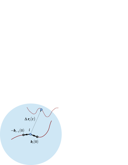
Figure 3: Sketch of the i-th monomer displacement $\Delta\mathbf{r}_{i}(t)$ in a time $t$ and the initial orientations of the bonds with the adjacent monomers of a linear chain molecule. Maximum correlation of $\Delta\mathbf{r}_{i}(t)$ with the initial orientations of the bonds is reached when the former is of the order of the bond length. At later times the correlation decay slowly and is not negligible if the monomer displaces by less than the radius of the colored sphere, about five times the bond length, see Sec.3.2.2.

3.2 Connectivity anisotropy (COA)

3.2.1 Definition

Let us consider a melt of $N_{c}$ linear polymer chains with $M$ monomers and $M-1$ bonds. The i-th monomer has position $\mathbf{r}_{i}(t)$ at time $t$. It is linked to the neighbouring monomers by bonds $\mathbf{b}_{i-1}(t)$ and $\mathbf{b}_{i}(t)$ with fixed length $b$, see Fig.3, where:

$$\mathbf{b}_{i}(t)=\mathbf{r}_{i+1}(t)-\mathbf{r}_{i}(t)\qquad 1\leq i\leq M-1$$ (3)

We consider the monomer displacement in a time $t$, $\Delta\mathbf{r}_{i}(t)\equiv\mathbf{r}_{i}(t)-\mathbf{r}_{i}(0)$, and its modulus $\left|\Delta\mathbf{r}_{i}(t)\right|$, see Fig.3. We define the following correlation function between the direction of the monomer displacement in a time $t$ and the initial orientation of the bonds linking the monomer to the adjacent ones ($\mathbf{b}_{i}\equiv\mathbf{b}_{i}(0)$):

$$\widehat{C}(t)=\left\langle\frac{1}{2}\frac{1}{M-1}\sum_{i=1}^{M}\frac{\Delta\mathbf{r}_{i}(t)}{\left|\Delta\mathbf{r}_{i}(t)\right|}\cdot\frac{({\bf b}_{i}-{\bf b}_{i-1})}{b}\right\rangle_{N_{c}}$$ (4)

It is understood that ${\bf b}_{M}={\bf b}_{0}=0$. The definition is independent of the choice of the end monomer labelled as $i=1$. The sum in Eq.4 is divided by twice the total number of bonds per chain. Henceforth, $\widehat{C}(t)$ will be referred to as the connectivity anisotropy function.

$\widehat{C}(t)$ vanishes at both short and long times. In fact, at short times the monomer displacement is ballistic, whereas at long times it is diffusive. In both regimes the displacement direction is not correlated with the initial bond arrangement. To better appreciate the major features of $\widehat{C}(t)$, it is worthwhile to define the companion function:

$$\widetilde{C}(t)=\frac{b}{2\,\langle\left|\Delta\mathbf{r}_{m}(t)\right|\rangle}\,\left[1-C_{bb}(t)\right]$$ (5)

$\widetilde{C}(t)$ is derived in A. It is an effective approximation of the connectivity anisotropy function $\widehat{C}(t)$, see Sec.3.2.2. Since $C_{bb}(t)$ vanishes at long times, see Fig.2, $\widetilde{C}(t)$ decays as:

$$\widetilde{C}(t)\simeq\frac{b}{2\;\langle\left|\Delta\mathbf{r}_{m}(t)\right|\rangle}$$ (6)

At long times in the diffusive regime, $\left|\Delta\mathbf{r}_{m}(t)\right|\simeq\langle\Delta r^{2}(t)\rangle^{1/2}\simeq\alpha\,t^{1/2}$ with $\alpha=R_{ee}\tau_{D}^{-1/2}$ from Eq.1. Then, Eq.6 yields:

$$\widetilde{C}(t)\simeq\frac{b}{2\;R_{ee}}\;\left(\frac{\tau_{D}}{t}\right)^{1/2}\hskip 17.07164ptt\gg\tau_{D}$$ (7)

Eq.7 emphasizes the slow decay of the connectivity anisotropy function.

The derivation of $\widetilde{C}(t)$ does not make any assumption on the chain length. However, to provide more insight into our results, it proves useful to derive in B the short-chain limit of $\widetilde{C}(t)$. To this aim, we neglect the role of the entanglements and resort to the Rouse gaussian theory of polymer dynamics which pictures the chains as ”phantoms”, i.e. perfectly crossable, and dissolved in a structureless environment [9, 10, 11, 71]. The short-chain limit of $\widetilde{C}(t)$ will be denoted as $\widetilde{C}^{R}(t)$.

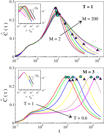
Figure 4: Connectivity anisotropy function $\widehat{C}(t)$, Eq.4. Top: dependence on the chain length for $T=1$. Bottom: dependence on the temperature for trimers ($M=3$). Symbols and color codes as in Fig.1. The insets of the two panels focus on the long-time part confirming the asymptotic decay predicted by Eq.7. $\widehat{C}(t)$ reaches the maximum at $\tau_{max}$ (cyan squares) when the monomer displaces by one diameter on average (see Fig.1). Note that the position and the height of the maximum are nearly independent of the chain length. The maximum height and the residual correlations at the onset of the diffusive regime at $\tau_{D}$ (violet triangles) are nearly independent of the temperature.

3.2.2 Results

Fig.4 plots the connectivity anisotropy function $\widehat{C}(t)$, Eq.4. It is seen that $\widehat{C}(t)$ vanishes at short times, owing to the initial missing correlations between the directions of the displacement and the bond orientation. Only a small bump is observed at $t\sim 0.175$, the average time needed to reverse the particle velocity by collisions with the cage of the first neighbours (see Sec.3.3.3 and Fig.10), signalling the weak influence of the local order on $\widehat{C}(t)$. Later, a peak is observed at $\tau_{max}$, where $\widehat{C}(t)$ is maximum. Both the position and the height of the peak are nearly independent of the chain length, see Fig.4 (top). This is understood by noting that the monomer displaces only by about one bond length on average at $\tau_{max}$, see Fig.1, and, therefore, does not experience the constraints posed by all the connected structure. At longer times $\widehat{C}(t)$ decreases, more slowly for longer chains, and finally vanishes as $\widehat{C}(t)\sim t^{-1/2}$ for $t\gg\tau_{D}$, see Fig.4 (insets), in agreement with the long-time decay predicted by Eq.7. Note that the maximum height and the residual correlations at the onset of the diffusive regime at $\tau_{D}$ are nearly independent of the temperature, see Fig.4 (bottom).

It is customarily said that the correlations in a polymer melt vanish when the chain moves it own size $\sim R_{ee}$. This statement is scrutinized in Fig.4 where the violet triangles mark the residual anisotropy at time $\tau_{D}$, i.e. the time needed to displace a monomer of $R_{ee}$, see Eq.1. It is seen that $\widehat{C}(\tau_{D})$ is not negligible for $M\lesssim 15$ since it exceeds $0.1$. In particular, $\widehat{C}(\tau_{D})\sim 0.12$ for a decamer. This residual correlation is captured by $\widetilde{C}(\tau_{D})$, Eq.7. In fact, by reminding the chain-length dependence of the end-end distance, see Sec.3.1, one finds $\widetilde{C}(\tau_{D})\sim b/(2R_{ee})=1/\sqrt{4C_{\infty}(M-1)}\sim 0.14$ for $M=10$, in good agreement with $\widehat{C}(\tau_{D})$.

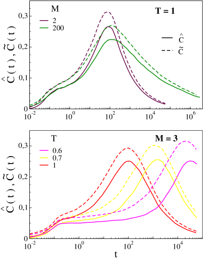
Figure 5: Comparison of the anisotropy function $\widehat{C}(t)$, Eq.4, with the first-order approximation, $\widetilde{C}(t)$, Eq.5, for selected chain lengths (top) and temperatures (bottom).

The good agreement at $\tau_{D}$ prompts us to compare at any time the exact connectivity anisotropy function $\widehat{C}(t)$, Eq.4, and the first-order approximation $\widetilde{C}(t)$, Eq.5. The results are shown in Fig.5. It is seen that the agreement is satisfactory with average deviations of about 15 $\%$.

Eq.6 suggests that the anisotropy of the random walk, after the maximum at $\tau_{max}$, decays at $0.1$ when the monomer displaces on average by five bond lengths, corresponding to about four particle diameters, independently of the chain length. The prediction is satisfactory. Indeed, by inspecting Fig.1 and Fig.4, one finds that $\widehat{C}(t)=0.1$ if the root mean square displacement $\simeq 4.61$ bond lengths, for all the chain lengths under study. Fig.3 provides a pictorial representation of the situation. The finding may be also expressed in terms of the Kuhn length $\ell_{K}$, the local stiffness of the polymer chain, to get rid of the details of the MD model and resort to a quantity experimentally accessible. It is found [10]:

$$\ell_{K} \equiv \frac{R^{2}_{ee}}{(M-1)b}$$

$$= C_{\infty}\,b$$

$$= 1.51\;b$$

One concludes that the anisotropy of the random walk due to the connectivity is not negligible over monomer displacements as large as about three Kuhn segments. Notice that two sites of the same chain have correlated geometry if they are spaced by about one Kuhn length. This means that the spatial decay of the anisotropy is not driven by the local stiffness of the chain but it follows from the slow spatial decay of the correlations, Eq.6.

Fig.6 compares the connectivity anisotropy function, $\widehat{C}(t)$, with the short-chain limit $\widetilde{C}^{R}(t)$, derived in B. $\widetilde{C}^{R}(t)$ is smaller at short times, $t\lesssim 10$. This is readily interpreted by reminding that $\widetilde{C}^{R}(t)$ is derived in terms of the Rouse theory, which pictures the chain surroundings as structureless [9, 71], thus it misses the enhancement of the anisotropy due to local order, see Sec.3.3. The agreement between $\widetilde{C}^{R}(t)$ and the connectivity anisotropy function $\widehat{C}(t)$ becomes extremely good for $t\gtrsim 10$ and $M=3,15$. For $M=200$, $\widetilde{C}^{R}(t)$ underestimates $\widehat{C}(t)$ after the maximum. This is clear evidence that the COA loss is slowed down by the presence of chain entanglements which are neglected by $\widetilde{C}^{R}(t)$, relying on the Rouse theory which pictures the chains as ”phantoms”, i.e. perfectly crossable [9, 71]. For the present models entanglements play a significant role for $M\gtrsim 80$, see Sec.2.

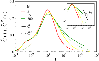
Figure 6: Comparison of the connectivity anisotropy function, $\widehat{C}(t)$, with the short-time limit ${\widetilde{C}}^{R}(t)$, Eq.20 with $\kappa=0.725$, for selected chain lengths and $T=1$. Color codes as in Fig.1. The inset focus on the long-time decay. The characteristic time $\tau$ of Eq.22 and Eq.23 has been set to match the peak position of $\widehat{C}(t)$, whereas the parameter $\kappa$ has been adjusted to best-fit Eq.20 to the results for $M=3$. The values of both $\tau$ and $\kappa$ are the same for $M=3,15,200$. Note that ${\widetilde{C}}^{R}(t)$ agrees very nicely with $\widehat{C}(t)$ for $t\gtrsim 10$ and $M=3,15$. It underestimates the connectivity anisotropy at short times and, for $M=200$, at long times.

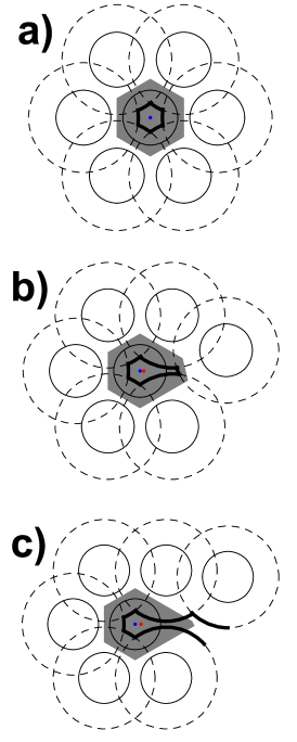
Figure 7: Schematic 2D view of a particle trapped by the cage of six first neighbours. Particles are sketched as hard disks with continuous-lines. The Voronoi cell is the grey area. Note that the VP vertices are close to the voids between the particles. For a given - fixed - configuration of the first shell, the center of the trapped particle may span a well-defined free-volume represented by the region with thick borders. The region is built by noting that the centres of two hard disks cannot be closer than their diameter $d$. The dashed circles have radius $d$ and are the boundaries of the excluded regions to the central particle for each of the six neighbours. The three panels differ by different positions of the right-most particle. They refer to a ideally-ordered packed (top), deformed but still close (middle) and open (bottom) cage configurations. The blue dot is the position of the trapped particle which, together with the position of the surrounding particles, set the Voronoi cell with centroid of the vertices located at the red dot. The LOA axis is the line joining the blue dot with the red one (not drawn for clarity reasons). It provides a good indication of the direction along which the VP and the free-volume are deformed. Starting from a given seven-particle configuration, at later times the trapped particle tends to move initially along the LOA axis [63, 64]. The LOA axis is not defined in the extreme, and very rare [12], case of ideally-ordered cage.

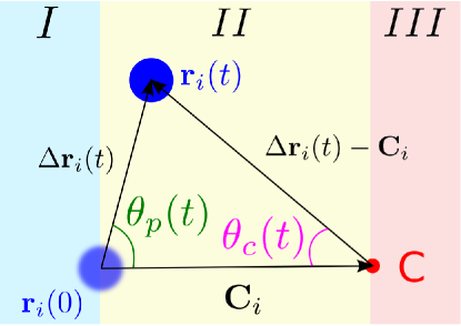
Figure 8: Quantities of interest to characterize the local-order anisotropies $\langle\cos\theta_{p}(t)\rangle$ and $\langle\cos\theta_{c}(t)\rangle$. Particle position at time $0$ and $t$ is marked by blue dots and the centroid of the VP vertices, Eq.9, at the initial time is marked by red dot. The highlighted regions are limited by planes perpendicular to $\mathbf{C}_{i}$ and passing through either the initial position of the particle or the centroid.

3.3 Local-order anisotropy (LOA)

Sec.3.2 discussed the COA anisotropy of the monomer random-walk which is maximum when the displacement is about the bond length. For smaller displacements the local order plays a major role to drive the anisotropy of the monomer displacement. The present Section investigates and discusses this aspect.

3.3.1 General aspects

LOA anisotropy is characterised in the present work by employing the vertices of the VP cell. That approach is well-known for atomic liquids [63] and granular matter [64] but, as far as we know, never applied to molecular liquid with competing COA anisotropy. The main motivation to concentrate on the VP vertices is that they are close to the voids between the particles and thus signal the weak spots of the cage, see Fig.7. To expose the correlation between the local order and the monomer dynamics, we consider the available free-volume. Rigorously, the geometrical free volume is defined as the volume over which the centre of the trapped sphere can translate, being fixed the cage configuration [75]. The VP cell and the free-volume region are, in general, not coinciding even if they exhibit some qualitative resemblance, e.g. see the examples of well-packed, Fig.7(a), mildly, Fig.7(b), and heavily distorted, Fig.7(c), cages. Cages are usually quite distorted in both atomic and molecular liquids [12]. The distortion is due to defective packing leading to the opening of one weak spot of the cage, or more. As an example, Fig.7 sketches three snapshots of an elementary opening process due to the rearrangement of one single member of the first shell. It is seen that the VP vertices being closer to the rearranging member approach the widening weak spot. The centroid, the center of mass of the VP vertices, does the same. Fig.7 shows that, for a given distorted cage, the free-volume is distorted too and the elongation of the free-volume occurs nearly along the same axis of the VP cell. This axis is approximated by the LOA axis, the line joining the centroid with the centre of the trapped monomer [63, 64]. The importance of the LOA axis resides in the previous finding [63, 64], which may be hinted at in Fig.7 and will be substantiated in Sec.3.3.3 for a molecular liquid as well, that, starting from a given configuration at $t_{0}$, at later times the trapped particle tends to move initially along the LOA axis set at $t_{0}$.

3.3.2 Definition

On the basis of the discussion in Sec.3.3.1, we define LOA axis at the initial time as [63, 64]:

$$\hat{\bf u}^{C}_{i}=\frac{\mathbf{C}_{i}}{|\mathbf{C}_{i}|}$$ (8)

$\mathbf{C}_{i}$ is the position of the centroid, the center of mass of the VP vertices, with respect to the position of the $i$-th particle at the initial time, see Fig.8:

$$\mathbf{C}_{i}=\frac{1}{N_{v,\,i}}\sum_{j=1}^{N_{v,\,i}}\mathbf{v}^{j}_{i}$$ (9)

where $N_{v,\,i}$ and $\mathbf{v}^{j}_{i}$ are the number of vertices and the position of the VP $j$-th vertex with respect to the position of the $i$-th particle at the initial time, respectively.

In order to investigate the LOA anisotropy of the i-th particle we investigate two distinct order parameters. First, following previous studies [63, 64], we consider the correlation between the LOA axis set at the initial time and the direction of the displacement of the $i$-th monomer in a time lapse $t$, $\hat{\bf u}_{i}(t)\equiv\Delta\mathbf{r}_{i}(t)/\left|\Delta\mathbf{r}_{i}(t)\right|$, see Fig.8:

$$\langle\cos\theta_{p}(t)\rangle=\frac{1}{N}\sum_{i=1}^{N}\hat{\bf u}_{i}(t)\cdot\hat{\bf u}^{C}_{i}$$ (10)

Furthermore, we also consider the correlation between the LOA axis set at the initial time and the direction of the particle position at time $t$ with respect to the centroid position at the initial time, $\big{[}\Delta\mathbf{r}_{i}(t)-\mathbf{C}_{i}\big{]}/\big{|}\Delta\mathbf{r}_{i}(t)-\mathbf{C}_{i}\big{|}$, see Fig.8:

$$\langle\cos\theta_{c}(t)\rangle=\frac{1}{N}\sum_{i=1}^{N}\frac{\big{[}\Delta\mathbf{r}_{i}(t)-\mathbf{C}_{i}\big{]}}{\big{|}\Delta\mathbf{r}_{i}(t)-\mathbf{C}_{i}\big{|}}\cdot\big{[}-\hat{\bf u}^{C}_{i}\big{]}$$ (11)

Complete isotropy yields $\langle\cos\theta_{i}\rangle=0$ ($i=p,c$). Perfect alignment of $\hat{\bf u}_{i}(t)$ with respect to $\hat{\bf u}^{C}_{i}$ yields $\langle\cos\theta_{p}\rangle=1$ whereas perfect alignment of $\big{[}\Delta\mathbf{r}_{i}(t)-\mathbf{C}_{i}\big{]}$ with respect to $-\hat{\bf u}^{C}_{i}$ yields $\langle\cos\theta_{c}\rangle=1$. Furthermore, if the monomer displacement is large with respect to $|\mathbf{C}_{i}|$, $\theta_{p}(t)\simeq\pi-\theta_{c}(t)$ and $\langle\cos\theta_{p}(t)\rangle\approx-\langle\cos\theta_{c}(t)\rangle$. The order parameters defined by Eq.10 and Eq.11 provide complementary information. By referring to Fig.8, positive values of $\langle\cos\theta_{c}(t)\rangle$ signal that the particle is preferentially located in regions I and II, whereas positive values of $\langle\cos\theta_{p}(t)\rangle$ denote preferential location of the particle in regions II and III. Fig.7 suggests that regions I and III are populated, initially, by monomers well inside the cage and close to the weak spots of the cage, respectively, being region II a transition zone.

It must be pointed out that the anisotropies $\langle\cos\theta_{p}(t)\rangle$ and $\langle\cos\theta_{c}(t)\rangle$ are not restricted to polymer systems, but are well-defined for atomic liquids too.

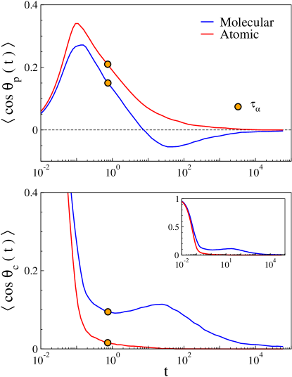
Figure 9: Comparison between the local-order anisotropies $\langle\cos\theta_{p}(t)\rangle$ (top) and $\langle\cos\theta_{c}(t)\rangle$ (bottom) in a melt of trimers (blue) and an atomic liquid (red) with the same temperature ($T=1.5$) and density. The inset in the bottom panel shows the complete decay of $\langle\cos\theta_{c}(t)\rangle$.

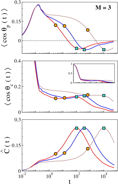
Figure 10: Local-order anisotropies , $\langle\cos\theta_{p}(t)\rangle$ (top) and $\langle\cos\theta_{c}(t)\rangle$ (middle) for trimers at different temperatures. The inset of the middle panel shows the full decay of $\langle\cos\theta_{c}(t)\rangle$. For comparison, the corresponding connectivity anisotropy $\widehat{C}(t)$ is plotted in the bottom panel. Symbols and color codes as in Fig.1.

3.3.3 Results

To provide comparison with, and extend, previous studies about $\langle\cos\theta_{p}(t)\rangle$ in atomic liquids [63], Fig.9 compares the LOA anisotropies of the melt of trimers under study and an atomic liquid with the same temperature and density. Let us start just with $\langle\cos\theta_{p}(t)\rangle$, Eq.10. It is plotted in Fig.9 (top). At very short times the direction of the particle displacement $\hat{\bf u}_{i}(t)$ is almost isotropic and $\langle\cos\theta_{p}(t)\rangle$ is small. Referring to Fig.7, this corresponds to the early stage of the cage exploration by the trapped monomer. Later, $\langle\cos\theta_{p}(t)\rangle$ increases and reaches the maximum at $t\sim 0.175$. One notices that, for both the molecular and the atomic liquids, the maximum corresponds to the minimum of the velocity correlation function (not shown), i.e. the time needed by most particles to reverse their initial velocity due to the collision with the cage of the first neighbours. The presence of a well-defined maximum of $\langle\cos\theta_{p}(t)\rangle$ confirms also for a molecular liquid the initial tendency of the trapped particle to move along the LOA axis already evidenced in atomic [63] and granular matter [64]. It is clear indication that initially there is correlation between the local structure and the particle displacement. The reduction of the maximum of $\langle\cos\theta_{p}(t)\rangle$ from the ideal unit value is manifestation of the partial misalignment of the monomer displacement with respect to the LOA axis. Interestingly, the connectivity acts as a constraint in the rattling motion of the monomer inside the cage, due to the bonds linking the trapped monomer to one or two of the closest monomers. This results in additional misalignment, thus leading to the decrease of the maximum of $\langle\cos\theta_{p}(t)\rangle$ of $\sim 20\%$ with respect to the atomic liquid. After the maximum the anisotropy $\langle\cos\theta_{p}(t)\rangle$ decreases and vanishes in a monotonous way in the atomic liquid. Differently, in the liquid of trimers a minimum is observed. This regime, which is controlled by the connectivity, will be analysed in detail below. We now discuss $\langle\cos\theta_{c}(t)\rangle$, Eq.11 plotted in Fig.9 (bottom). At very short times the displacement $\Delta\mathbf{r}_{i}(t)$ is small and $\langle\cos\theta_{c}(t)\rangle\sim 1$. Then, the anisotropy drops up to $t\sim 0.175$ where a knee is observed. The knee corresponds to the maximum of $\langle\cos\theta_{p}(t)\rangle$. For longer times $\langle\cos\theta_{c}(t)\rangle$ vanishes at about $\tau_{\alpha}$ in the atomic liquid whereas it persists at much longer times in the liquid of trimers. This regime, which is controlled by the connectivity, will be analysed in detail below. All in all, Fig.9 suggests that, even for times shorter than the structural relaxation time the influence of the local order on the monomer displacement is partially decreased by the connectivity, at longer times the latter favours the persistence of the local order.

Fig.10 examines in detail the LOA anisotropies of the liquid of trimers. Fig.10 (top) plots $\langle\cos\theta_{p}(t)\rangle$ at different temperatures. It is seen that the region around the maximum is virtually unaffected by the temperature changes, whereas for $t\gtrsim 0.7$ a significant slowing-down is observed by decreasing the temperature. A similar behaviour is observed in $\langle\cos\theta_{c}(t)\rangle$, see Fig.10 (middle) even if the influence of the temperature appears earlier in time since it is already visible after the knee at $t\sim 0.175$. At times longer than the structural relaxation time a minimum of $\langle\cos\theta_{p}(t)\rangle$ is observed in coincidence with the local maximum of $\langle\cos\theta_{c}(t)\rangle$. The coincidence follows by the approximate relation $\langle\cos\theta_{p}(t)\rangle\approx-\langle\cos\theta_{c}(t)\rangle$, which holds at long times, see Sec.3.3.2. By comparison with the connectivity anisotropy function $\widehat{C}(t)$, Fig.10 (bottom) one realises that the minimum of $\langle\cos\theta_{p}(t)\rangle$ and the local maximum of $\langle\cos\theta_{c}(t)\rangle$ just mirror the region of the COA maximum which occur for monomer displacements of about one bond length, see Fig.1.

Fig.9 and Fig.10 encompass our results about LOA and COA. At short times, before the structural relaxation, connectivity and local order play different roles. In fact, the connectivity is antagonistic and decreases LOA, Fig.9 (top), viceversa, COA is slightly enhanced by the local order, Fig.10 (bottom). After structural relaxation, the connectivity ensures the persistence of LOA up to displacements as large as about one bond length, or one particle diameter, Fig.9 (bottom) and Fig.10 (middle).

It is interesting to interpret the localization of the monomer in the three regions defined in Fig.8 in the light of our results on LOA anisotropy. At very short times the monomer is mainly in region I and, sligthly more, in region II ( $\langle\cos\theta_{p}(t)\rangle$ and $\langle\cos\theta_{c}(t)\rangle$ both positive). Then, the monomer approaches the centroid and region II and region III become more populated. As a result, $\langle\cos\theta_{p}(t)\rangle$ increases up to the maximum and $\langle\cos\theta_{c}(t)\rangle$ decreases. After the structural relaxation $t\gtrsim\tau_{\alpha}$, the direction of the monomer displacement with respect to both the original position and the centroid, randomises in the atomic liquid, yielding the monotonous loss of LOA anisotropy, see Fig.9. Instead, in the molecular liquid where COA is present, both the change of sign of $\langle\cos\theta_{p}(t)\rangle$ and the increase of $\langle\cos\theta_{c}(t)\rangle$ following the structural relaxation, see Fig.9 and Fig.10, suggest that the bonds resist the randomization of the monomer displacement and tend to pull back the monomer, thus enriching the monomer population in region I. The strength of the effect is driven by COA since the latter is a measure of the correlation between the monomer displacement and the arrangements of the bonds tethering the monomer to the adjacent ones, see Sec.3.2.1.

The above results about LOA provide insight into our previous finding that the rattling amplitude of the monomer in the cage of the closest neighbours has poor correlation with the cage shape in the same liquid of trimers under study here [23, 24]. The mean square rattling amplitude was evaluated as the MSD at $t\simeq 1$, a quantity exhibiting universal correlation with the structural relaxation [13, 14, 15, 16, 17, 18, 19, 20, 21, 22]. We now see in Fig.10 that the LOA anisotropies, $\langle\cos\theta_{p}(t)\rangle$ and $\langle\cos\theta_{c}(t)\rangle$ are rather small at $t\simeq 1$. The small LOA value strongly suggests that the sole consideration of the local scale is not enough to understand the microscopic origin of the rattling amplitude of the trapped monomer in the cage, in agreement with previous conclusions pinpointing the major role of collective effects on larger length scales [25, 26, 27].

The consideration of linear chains longer than trimers changes only qualitatively the conclusions reached up to now about the interplay between LOA and COA. For conciseness, they are only briefly summarized. For times shorter than $\tau_{\alpha}$ the key parameter is the average effective number of bonds per monomer $2(1-1/M)$ [12], so that the effective bond constraint on the rattling motion in the cage increases with the chain length. As a result, the maximum of $\langle\cos\theta_{p}(t)\rangle$ decreases by increasing the chain length, a finding that is readily interpreted by reminding that the connectivity disturbs the alignment of the monomer displacement with the LOA axis, see Fig.9 (top). For times longer than than $\tau_{\alpha}$ we know that the COA maximum increases with the chain length and the decay is slowed down, see Fig.4. As a consequence, being the LOA anisotropies driven by COA at intermediate and long times, the local maximum of $\langle\cos\theta_{c}(t)\rangle$ increases, the local minimum of $\langle\cos\theta_{p}(t)\rangle$ decreases and their decay at long times slows down.

4 Conclusions

Extensive MD simulations on melts of linear fully-flexible chains ranging from dimers up to entangled polymers are performed to investigate the anisotropy of the monomer random walk. We consider the roles of both the local geometry and the connectivity.

We first scrutinise the connectivity anisotropy (COA), the correlation between the initial bond orientation and the subsequent direction of the monomer displacement. At times comparable with the time needed by most particles to reverse their initial velocity due to the collision with the cage of the first neighbours, local order tends to enhance slightly COA. Later, we find the peculiar non-monotonous time-dependence of COA, peaking when the monomer displacement is of the order of the bond length and vanishing as $t^{-1/2}$ at longer times. COA is slowed down by the chain entanglements and becomes negligible when the displacements is as large as about five bond lengths, i.e. about four monomer diameters or three Kuhn lengths.

As to the local-order anisotropy (LOA), attention is paid to the LOA axis, the line joining at a given time $t_{0}$ the positions of the monomer trapped in the cage of the first neighbours and the related VP centroid, providing indications on the initial direction of the monomer displacement at times later than $t_{0}$. We consider two complementary LOA metrics by correlating the LOA axis at $t_{0}$ with the subsequent time evolution of the directions of either the monomer displacement or the particle position with respect to the initial centroid position. We conclude, also by comparison with a reference atomic liquid, that at times shorter than $\tau_{\alpha}$ LOA is affected by the shape of the cage of the closest neighbours with antagonistic effect by the connectivity. Differently, after structural relaxation, the connectivity favours the persistence of LOA up to displacements as large as about one bond length, or one particle diameter.

Our results strongly suggest that the sole consideration of the local order is not enough to understand the microscopic origin of the rattling amplitude of the trapped monomer in the cage of the neighbours.

Appendix A Derivation of the function $\widetilde{C}(t)$, Eq. 5

The function $\widetilde{C}(t)$, Eq. 5, is an approximation of the connectivity anisotropy function $\widehat{C}(t)$, Eq.4. The latter has the form $\widehat{C}(t)=\langle X_{m}/Y_{m}\rangle$ where $X_{m}$ and $Y_{m}$ are quantities referred to the $m$-th monomer:

$$X_{m} = \Delta\mathbf{r}_{m}(t)\cdot\frac{({\bf b}_{m}-{\bf b}_{m-1})}{b}\frac{M}{2(M-1)}$$ (12)

$$Y_{m} = \left|\Delta\mathbf{r}_{m}(t)\right|$$ (13)

and the brackets denotes the average over all the monomers, that is

$$\left\langle Z_{m}\right\rangle=\left\langle\frac{1}{M}\sum_{i=1}^{M}Z_{i}\right\rangle_{N_{c}}$$ (14)

One evaluates the ratio $X_{m}/Y_{m}$ by expanding the random variables $X_{m}$ and $Y_{m}$ around their averages [76]. At first order, after suitable average, one has $\widehat{C}(t)=\langle X_{m}/Y_{m}\rangle\simeq\langle X_{m}\rangle/\langle Y_{m}\rangle\equiv\widetilde{C}(t)$ with :

$$\widetilde{C}(t)=\frac{b}{\langle\left|\Delta\mathbf{r}_{m}(t)\right|\rangle}\,C(t)$$ (15)

where

$$C(t)=\left\langle\frac{1}{2}\frac{1}{M-1}\frac{1}{b^{2}}\sum_{i=1}^{M}\Delta\mathbf{r}_{i}(t)\cdot({\bf b}_{i}-{\bf b}_{i-1})\right\rangle_{N_{c}}$$ (16)

The function $C(t)$ is recast as:

$$C(t)=\frac{1}{2}[1-C_{bb}(t)]$$ (17)

To prove Eq.17, we notice that the difference of the displacements of the two adjacent monomers $i$ and $i+1$ is:

$$\Delta\mathbf{r}_{i}(t)-\Delta\mathbf{r}_{i+1}(t)={\bf b}_{i}-{\bf b}_{i}(t)$$ (18)

Let us consider the sum in Eq.16. Inserting Eq.18 and setting ${\bf b}_{M}={\bf b}_{0}=0$ yield:

$$\displaystyle\sum_{i=1}^{M}\Delta\mathbf{r}_{i}(t)\cdot\big{(}{\bf b}_{i}-{\bf b}_{i-1}\big{)}=$$

$$\Delta\mathbf{r}_{1}(t)\cdot{\bf b}_{1}+\Delta\mathbf{r}_{2}(t)\cdot\big{(}{\bf b}_{2}-{\bf b}_{1}\big{)}+\ldots+\Delta\mathbf{r}_{M}(t)\cdot(-{\bf b}_{M-1})=$$

$$\Big{[}\Delta\mathbf{r}_{1}(t)-\Delta\mathbf{r}_{2}(t)\Big{]}\cdot{\bf b}_{1}+\ldots+\Big{[}\Delta\mathbf{r}_{M-1}(t)-\Delta\mathbf{r}_{M}(t)\Big{]}\cdot{\bf b}_{M-1}=$$

$$\Big{[}{\bf b}_{1}-{\bf b}_{1}(t)\Big{]}\cdot{\bf b}_{1}+\ldots+\Big{[}{\bf b}_{M-1}-{\bf b}_{M-1}(t)\Big{]}\cdot{\bf b}_{M-1}=$$

$$\displaystyle\sum_{i=1}^{M-1}{\bf b}_{i}^{2}-\Big{[}{\bf b}_{i}(t)\cdot{\bf b}_{i}\Big{]}=$$

$$\Big{[}M-1\Big{]}b^{2}-b^{2}\displaystyle\sum_{i=1}^{M-1}\frac{{\bf b}_{i}(t)\cdot{\bf b}_{i}}{b^{2}}$$ (19)

Plugging Eq. 19 into Eq. 16 recovers Eq.17 :

$$C(t) = \left\langle\frac{1}{2}-\frac{1}{2}\frac{1}{M-1}\sum_{i=1}^{M-1}\frac{{\bf b}_{i}(t)\cdot{\bf b}_{i}}{b^{2}}\right\rangle_{N_{c}}$$

$$= \frac{1}{2}\Big{[}1-C_{bb}(t)\Big{]}$$

By plugging Eq.17 into Eq.15, one recovers Eq.5 .

Appendix B Short-chain limit of $\widetilde{C}(t)$

We specialise $\widetilde{C}(t)$, Eq.5, to short chains, i.e. we neglect the role of the chain entanglements. To this aim, one considers the Rouse gaussian theory of polymer dynamics which pictures the chains as ”phantoms”, i.e. perfectly crossable, and dissolved in a structureless environment [9, 71]. The Rouse approximated expression of the connectivity anisotropy function will be denoted as $\widetilde{C}^{R}(t)$ and defined by:

$$\widetilde{C}^{R}(t)=\kappa\,\frac{b}{2}\,\left[\frac{3\pi}{8\,\langle\Delta r^{2}(t)\rangle^{R}}\right]^{1/2}\,\left[1-C^{R}_{bb}(t)\right]$$ (20)

The above equation, with $\kappa=1$, is Eq. 5 by taking into account that for gaussian displacements, one assumption of the Rouse theory [9, 71], $\langle\left|\Delta\mathbf{r}_{m}(t)\right|\rangle=\sqrt{8/3\pi}\,\langle\Delta r^{2}(t)\rangle^{1/2}$. $\kappa$ is an adjustable parameter, independent of the chain length, to correct the approximations inherent in both the Rouse approach and the derivation of $\widetilde{C}(t)$. $C_{bb}^{R}(t)$ and $\langle\Delta r^{2}(t)\rangle^{R}$ are the expressions of $C_{bb}(t)$ and MSD in the framework of the Rouse theory, respectively [9, 71]:

$$C_{bb}^{R}(t) = \frac{1}{(M-1)}\sum_{p=1}^{M-1}\phi^{R}_{p}(t)$$ (21)

$$\langle\Delta r^{2}(t)\rangle^{R} = \frac{b^{2}}{2M}\left[\frac{t}{\tau}+\sum_{p=1}^{M-1}\frac{1-\phi^{R}_{p}(t)}{\sin^{2}(p\pi/2M)}\right]$$ (22)

where $\tau$ is a characteristic time, independent of the chain length, and $\phi^{R}_{p}(t)$ denotes the correlation function of the $p$-th Rouse mode [9, 71]:

$$\phi^{R}_{p}(t)=\exp\left[-\sin^{2}(p\pi/2M)\,\frac{t}{\tau}\right]$$ (23)

Eq.21 and Eq.22 are derived by first expressing the monomer positions in terms of the Rouse orthogonal normal modes and then averaging the results over all the monomers [9, 71].

References

- [1] J. P. Hansen and I. R. McDonald. Theory of Simple Liquids, 3rd Ed. Academic Press, 2006.
- [2] W. Götze. Complex Dynamics of Glass-Forming Liquids: A Mode-Coupling Theory. Oxford University Press, Oxford, 2008.
- [3] Ludovic Berthier and Giulio Biroli. Theoretical perspective on the glass transition and amorphous materials. Rev. Mod. Phys., 83:587–645, 2011.
- [4] Wolfgang Paul and Grant D Smith. Structure and dynamics of amorphous polymers: computer simulations compared to experiment and theory. Rep. Prog. Phys., 67:1117–1185, 2004.
- [5] J. Baschnagel and F. Varnik. Computer simulations of supercooled polymer melts in the bulk and in confined geometry. J. Phys.: Condens. Matter, 17:R851–R953, 2005.
- [6] Anuraag R. Kansal, S. Torquato, and F. H. Stillinger. Diversity of order and densities in jammed hard-particle packings. Phys. Rev. E, 66:041109, 2002.
- [7] T. Aste. Variations around disordered close packing. J. Phys.: Condens. Matter, 17:S2361–S2390, 2005.
- [8] T. Aste, M. Saadatfar, and T. J. Senden. Geometrical structure of disordered sphere packings. Phys. Rev. E, 71:061302, 2005.
- [9] M. Doi and S. F. Edwards. The Theory of Polymer Dynamics. Clarendon Press, Oxford, 1988.
- [10] M. Rubinstein and Ralph H. Colby. Polymer Physics. Oxford University Press, Oxford, 2003.
- [11] G. Strobl. The Physics of Polymers, III Ed. Springer, Berlin, 2007.
- [12] S. Bernini, F. Puosi, M. Barucco, and D. Leporini. Competition of the connectivity with the local and the global order in polymer melts and crystals. J. Chem. Phys., 139:184501, 2013.
- [13] L. Larini, A. Ottochian, C. De Michele, and D. Leporini. Universal scaling between structural relaxation and vibrational dynamics in glass-forming liquids and polymers. Nature Physics, 4:42–45, 2008.
- [14] A. Ottochian, C. De Michele, and D. Leporini. Universal divergenceless scaling between structural relaxation and caged dynamics in glass-forming systems. J. Chem. Phys., 131:224517, 2009.
- [15] F. Puosi and D. Leporini. Scaling between relaxation, transport, and caged dynamics in polymers: From cage restructuring to diffusion. J.Phys. Chem. B, 115:14046–14051, 2011.
- [16] F. Puosi, C. De Michele, and D. Leporini. Scaling between relaxation, transport and caged dynamics in a binary mixture on a per-component basis. J. Chem. Phys., 138:12A532, 2013.
- [17] C. De Michele, E. Del Gado, and D. Leporini. Scaling between structural relaxation and particle caging in a model colloidal gel. Soft Matter, 7:4025–4031, 2011.
- [18] D. S. Simmons, M. T. Cicerone, Q. Zhong, M. Tyagic, and J. F. Douglas. Generalized localization model of relaxation in glass-forming liquids. Soft Matter, 8:11455–11461, 2012.
- [19] Beatriz A. Pazmiño Betancourt, Paul Z. Hanakata, Francis W. Starr, and Jack F. Douglas. Quantitative relations between cooperative motion, emergent elasticity, and free volume in model glass-forming polymer materials. Proc. Natl. Acad. Sci. USA, 112:2966–2971, 2015.
-
[20]
A. Ottochian and D. Leporini.
Scaling between structural relaxation and caged dynamics
in ca 0.4k 0.6(no 3) 1.4 and glycerol: free volume, time scales and implications for the pressure-energy correlations. Phil. Mag., 91:1786–1795, 2011. - [21] A. Ottochian and D. Leporini. Universal scaling between structural relaxation and caged dynamics in glass-forming systems: Free volume and time scales. J. Non-Cryst. Solids, 357:298–301, 2011.
- [22] A. Ottochian, F. Puosi, C. De Michele, and D. Leporini. Comment on “generalized localization model of relaxation in glass-forming liquids”. Soft Matter, 9:7890–7891, 2013.
- [23] S. Bernini, F. Puosi, and D. Leporini. Weak links between fast mobility and local structure in molecular and atomic liquids. J. Chem. Phys., 142:124504, 2015.
- [24] S. Bernini, F. Puosi, and D. Leporini. Cage rattling does not correlate with the local geometry in molecular liquids. J. Non-Cryst. Solids, 407:29–33, 2015.
- [25] F. Puosi and D. Leporini. Spatial displacement correlations in polymeric systems. J. Chem. Phys., 136:164901, 2012.
- [26] F. Puosi and D. Leporini. Erratum: “spatial displacement correlations in polymeric systems” [j. chem. phys.136, 164901 (2012)]. J. Chem. Phys., 139:029901, 2013.
- [27] L. Berthier and R. L. Jack. Structure and dynamics of glass formers: Predictability at large length scales. Phys. Rev. E, 76:041509, 2007.
- [28] G. Adam and J. H. Gibbs. On the temperature dependence of cooperative relaxation properties in glass-forming liquids. J. Chem. Phys., 43:139–146, 1965.
- [29] J. Dudowicz, K. F. Freed, and J. F. Douglas. Generalized entropy theory of polymer glass formation. Adv. Chem. Phys., 137:125–222, 2008.
- [30] Julian H. Gibbs and Edmund A. DiMarzio. Nature of the glass transition and the glassy state. J. Chem. Phys., 28:373–383, 1958.
- [31] Kang Chen, Erica J. Saltzman, and Kenneth S. Schweizer. Molecular theories of segmental dynamics and mechanical response in deeply supercooled polymer melts and glasses. Annu. Rev. Condens. Matter Phys., 1:277–300, 2010.
- [32] Vassiliy Lubchenko and Peter G. Wolynes. Theory of structural glasses and supercooled liquids. Annu. Rev. Phys. Chem., 58:235–266, 2007.
- [33] G Tarjus, S A Kivelson, Z Nussinov, and P Viot. The frustration-based approach of supercooled liquids and the glass transition: a review and critical assessment. J. Phys.: Condens. Matter, 17:R1143–R1182, 2005.
- [34] J. C. Dyre. The glass transition and elastic models of glass-forming liquids. Rev. Mod. Phys., 78:953–972, 2006.
- [35] S.V. Nemilov. Interrelation between shear modulus and the molecular parameters of viscous flow for glass forming liquids. J. Non-Cryst. Sol., 352:2715–2725, 2006.
- [36] F.W. Starr, S. Sastry, J. F. Douglas, and S. Glotzer. What do we learn from the local geometry of glass-forming liquids? Phys. Rev. Lett., 89:125501, 2002.
- [37] A. Lemaître. Structural relaxation is a scale-free process. Phys. Rev. Lett., 113:245702, 2014.
- [38] A.V. Granato. The specific heat of simple liquids. J. Non-Cryst. Solids, 307-310:376–386, 2002.
- [39] L. Yan, G. Düring, and M. Wyart. Why glass elasticity affects the thermodynamics and fragility of supercooled liquids. PNAS, 110:6307–6312, 2013.
- [40] V. N. Novikov, Y. Ding, and A. P. Sokolov. Correlation of fragility of supercooled liquids with elastic properties of glasses. Phys.Rev.E, 71:061501, 2005.
- [41] V. N. Novikov and A. P. Sokolov. Poisson’s ratio and the fragility of glass-forming liquids. Nature, 431(7011):961–963, 2004.
- [42] Stephen Mirigian and Kenneth S. Schweizer. Elastically cooperative activated barrier hopping theory of relaxation in viscous fluids.i. general formulation and application to hard sphere fluids. J. Chem. Phys., 140:194506, 2014.
- [43] Stephen Mirigian and Kenneth S. Schweizer. Elastically cooperative activated barrier hopping theory of relaxation in viscous fluids. ii. thermal liquids. J. Chem. Phys., 140:194507, 2014.
- [44] F. Puosi and D. Leporini. Correlation of the instantaneous and the intermediate-time elasticity with the structural relaxation in glassforming systems. J. Chem. Phys., 136:041104, 2012.
- [45] J. C. Dyre and W. H. Wang. The instantaneous shear modulus in the shoving model. J.Chem.Phys., 136:224108, 2012.
- [46] F. Puosi and D. Leporini. The kinetic fragility of liquids as manifestation of the elastic softening. Eur. Phys. J. E, 38:87, 2015.
- [47] S. Bernini and D. Leporini. Short-time elasticity of polymer melts: Tobolsky conjecture and heterogeneous local stiffness. J.Pol.Sci., Part B: Polym. Phys., 53:1401–1407, 2015.
- [48] Daniele Coslovich. Locally preferred structures and many-body static correlations in viscous liquids. Phys. Rev. E, 83:051505, 2011.
- [49] Simona Capponi, Simone Napolitano, and Michael Wübbenhorst. Supercooled liquids with enhanced orientational order. Nat. Commun., 3:1233, 2012.
- [50] Sadanand Singh, M. D. Ediger, and Juan J. de Pablo. Ultrastable glasses from in silico vapour deposition. Nat. Mater., 12:139–144, 2013.
- [51] A. Barbieri, G. Gorini, and D. Leporini. Role of the density in the crossover region of o-terphenyl and poly(vinyl acetate). Phys. Rev. E, 69:061509, 2004.
- [52] Glen M. Hocky, Daniele Coslovich, Atsushi Ikeda, and David R. Reichman1. Correlation of local order with particle mobility in supercooled liquids is highly system dependent. Phys. Rev. Lett., 113:157801, 2014.
- [53] Andrew J. Dunleavy, Karoline Wiesner, Ryoichi Yamamoto, and C. Patrick Royall. Mutual information reveals multiple structural relaxation mechanisms in a model glass former. Nat. Commun., 6:6089, 2015.
- [54] J. C. Conrad, F. W. Starr, and D. A. Weitz. Weak correlations between local density and dynamics near the glass transition. J.Phys. Chem. B, 109:21235–21240, 2005.
- [55] C. Patrick Royall, Stephen R. Williams, Takehiro Ohtsuka, and Hajime Tanaka. Direct observation of a local structural mechanism for dynamic arrest. Nat. Mater., 7:556–561, 2008.
- [56] Mathieu Leocmach and Hajime Tanaka. Roles of icosahedral and crystal-like order in the hard spheres glass transition. Nat. Commun., 3:974, 2012.
- [57] T. S. Jain and J. de Pablo. Role of local structure on motions on the potential energy landscape for a model supercooled polymer. J.Chem.Phys., 122:174515, 2005.
- [58] Christopher R. Iacovella, Aaron S. Keys, Mark A. Horsch, and Sharon C. Glotzer. Icosahedral packing of polymer-tethered nanospheres and stabilization of the gyroid phase. Phys. Rev. E, 75:040801(R), 2007.
- [59] N. C. Karayiannis, K. Foteinopoulou, and M. Laso. The structure of random packings of freely jointed chains of tangent hard spheres. J. Chem. Phys., 130(16):164908, 2009.
- [60] B. Schnell, H. Meyer, C. Fond, J.P. Wittmer, and J. Baschnagel. Simulated glass-forming polymer melts: Glass transition temperature and elastic constants of the glassy state. Eur. Phys. J. E, 34:97, 2011.
- [61] Makoto Asai, Mitsuhiro Shibayama, and Yasuhiro Koike. Common origin of dynamics heterogeneity and cooperatively rearranging region in polymer melts. Macromolecules, 44(16):6615–6624, 2011.
- [62] L. Larini, A. Barbieri, D. Prevosto, P. A. Rolla, and D. Leporini. Equilibrated polyethylene single-molecule crystals: molecular-dynamics simulations and analytic model of the global minimum of the free-energy landscape. J. Phys.: Condens. Matter, 17:L199–L208, 2005.
- [63] A. Rahman. Liquid structure and self-diffusion. J. Chem. Phys., 45:2585–2592, 1966.
- [64] Steven Slotterback, Masahiro Toiya, Leonard Goff, Jack F. Douglas, and Wolfgang Losert. Correlation between particle motion and voronoi-cell-shape fluctuations during the compaction of granular matter. Phys. Rev. Lett., 101:258001, 2008.
- [65] S. K. Sukumaran, G. S. Grest, K. Kremer, and R. Everaers. Identifying the primitive path mesh in entangled polymer liquids. J. Polym. Sci., Part B: Polym. Phys., 43:917–933, 2005.
- [66] M. Pütz, K. Kremer, and G. S. Grest. What is the entanglement length in a polymer melt? Europhys. Lett., 49:735–741, 2000.
- [67] Robert S. Hoy, Katerina Foteinopoulou, and Martin Kröger. Topological analysis of polymeric melts: Chain-length effects and fast-converging estimators for entanglement length. Phys. Rev. E, 80:031803, 2009.
- [68] G. S. Grest and K. Kremer. Molecular dynamics simulation for polymers in the presence of a heat bath. Phys. Rev. A, 33(5):3628–3631, 1986.
- [69] M. P. Allen and D. J. Tildesley. Computer simulations of liquids. Oxford university press, Clarendon, 1987.
- [70] S. Plimpton. Fast parallel algorithms for short-range molecular dynamics. J. Comput. Phys., 117:1–19, 1995.
- [71] A. Ottochian, D. Molin, A. Barbieri, and D. Leporini. Connectivity effects in the segmental self- and cross-reorientation of unentangled polymer melts. J. Chem. Phys., 131:174902, 2009.
- [72] A. Barbieri, E. Campani, S. Capaccioli, and D. Leporini. Molecular dynamics study of the thermal and the density effects on the local and the large-scale motion of polymer melts: Scaling properties and dielectric relaxation. J.Chem.Phys., 120:437–453, 2004.
- [73] Monojoy Goswami and Bobby G. Sumpter. Anomalous chain diffusion in polymer nanocomposites for varying polymer-filler interaction strengths. Phys. Rev. E, 81:041801, 2010.
- [74] Christoph Bennemann, Claudio Donati, Jorg Baschnagel, and Sharon C. Glotzer. Growing range of correlated motion in a polymer melt on cooling towards the glass transition. Nature, 399(6733):246–249, 05 1999.
- [75] S.Sastry, T.M. Truskett, P.G. Debenedetti, S.Torquato, and F.H.Stillinger. Free volume in the hard sphere liquid. Mol. Phys., 95:289–297, 1998.
- [76] T. Pham-Gia, N. Turkkan, and E. Marchand. Density of the ratio of two normal random variables and applications. Communications in Statistics - Theory and Methods, 35:1569–1591, 2006.