Heat transport in an anharmonic crystal

Abstract

We take an ordered, anharmonic crystal in the form of slab geometry in three dimensions. Apart from attaching baths of Langevin type to the extreme surfaces, we also attach baths of same type to the intermediate surfaces of the slab to simulate the environment surrounding the system. We assume noise functions to be Gaussian and their widths to be site dependent. We find that the radiated heat from the slab does not receive any correction at the leading order of anharmonic coupling and the Newton’s law of cooling holds for an appropriate choice of the widths. We observe that in the steady state limit entire slab becomes an assembly of $N$ different thermally equilibriated layers, where $N$ is the number of sites in the direction of conduction current flow. We find an exponentially falling nature of the temperature profile as its leading behaviour and its non-leading behaviour is governed by the two site dependent functions. Our evaluation suggests that in the thermodynamic limit thermal conductivity remains independent of the environment temperature and is dependent only on the difference of temperature of the extreme surfaces linearly at the leading order of anharmonic coupling. We find that owing to finiteness of conductivity in the thermodynamic limit, Fourier’s law holds to leading order in anharmonic coupling.

I Introduction

The process of heat transport in a solid mainly involves conduction, radiation and absorption of heat. When the absorption is absent in the steady state limit, the temperature profile of a solid bar falls exponentially from high to low temperature end of the bar if the radiated heat obeys Newton’s laws of cooling and the conducted current density obeys Fourier’s law:

$$\mathbf{J}(\mathbf{x})=-\kappa{\mathbf{\nabla}}T(\mathbf{x}),$$ (1)

where ${\mathbf{\nabla}}T(\mathbf{x})$ is the local temperature gradient and $\kappa$ is the thermal conductivity. In the steady state the exponentially falling nature of the temperature profile is experimentally verified by Ingen and HauszSaha1969 . Through ages it is a challenge to theoristBonetto2000 ; Lepri2003 to derive the laws involved with this process from the application of basic principles of statistical mechanics to a crystal of solid.

Our study is based on Langevin equation approachChaikin2009 ; Reif1985 which was first used to study heat conduction in ordered, harmonic lattice in one-dimensionRieder1967 . Later, this approach was used to study heat conduction in regular harmonic and anharmonic lattices in one, two and three dimensionsNakazawa1970 . This approach was also used to study heat conduction in disordered, harmonic system in oneRubin1971 ; Connor1974 ; Dhar2001 and twoLee2005 dimensions. This approach was adopted in disordered, harmonic system in two and three dimensionsChaudhuri2010 and the validity of Fourier’s law was numerically verified in pinned three dimensional system. The Fourier’s law was also verified numerically using this approach in three dimensional anharmonic crystalSaito2010 . Unlike the model of self consistent reservoirsBolsterli1970 ; Rich1975 ; Bonetto2004 , if one allows the heat to flow between intermediate surfaces and the attached baths, one derives Fourier’s law in three dimensional ordered harmonic system using this approach and obtains the exponentially falling temperature profile, provided that the radiated heat obeys the Newton’s law of coolingShila2013 .

In this paper we take the ordered, anharmonic crystal in three dimension in the form of slab geometry. Apart from the baths attached to the extremities, there are baths attached to the intermediate surfaces of the slab and the heat is allowed to flow between intermediate surfaces and the attached bathsShila2013 . We show using Langevin equation approach that Fourier’s law remains valid in the thermodynamic limit and a temperature dependent conductivity is obtained to leading order in anharmonic coupling. We observe that the radiated heat does not receive any correction form the anharmonic part. We obtain the exact temperature profile which is correct to leading order in anharmonic coupling and observe that the exponentially falling nature of the profile is modified by the two site dependent functions at the leading order in anharmonic coupling.

We organize the paper as follows. We discuss the model and obtain the steady state solution of the Langevin equation perturbatively to leading order in anharmonic coupling in section II. We compute the correlators in section III. We compute the radiated heat and obtain the temperature profile in section IV. We compute the conduction current density and obtain the Fourier’s law in section V. We summarize our results in section VII. We give a brief outline of the evaluation of frequency integrals in appendix A. We discuss the wave vector sums in the continuum limit in appendix B. We give the definition of the useful integrals and the required discrete sums in appendices C and D respectively.

II Model and its solution

We consider an anharmonic crystal in three dimensions and each lattice site ${\mathbf{n}}=(n_{1},\,n_{2},\,n_{3})$ is described by the three integers in the regions: $1\leq n_{1}\leq\,N$, $1\leq n_{2}\leq\,W_{2}$ and $1\leq n_{3}\leq\,W_{3}$. We attach Langevin type heat baths with the surfaces at $n_{1}=1$ and $n_{1}=N$ maintaining fixed temperatures $T_{1}$ and $T_{N}$ ($T_{1}\,>\,T_{N}$) respectively. Since the crystal is exposed to the surroundings, the mass points of the lattice interact with the environment. To simulate this interaction we also attach heat baths of the same type to the intermediate surfaces from $n_{1}=2$ to $n_{1}=N-1$. If $x_{{\mathbf{n}}}$ be the displacement field of a lattice site, the Lagrangian

$$L=m\sum_{\mathbf{n}}\frac{\dot{x}_{\mathbf{n}}^{2}}{2}-\sum_{{\mathbf{n}},\,\hat{e}}\Big{\{}\frac{C_{2}}{4}(x_{{\mathbf{n}}+\hat{e}}-x_{{\mathbf{n}}})^{2}+\frac{C_{4}}{8}(x_{{\mathbf{n}}+\hat{e}}-x_{{\mathbf{n}}})^{4}\Big{\}},$$ (2)

where $m$ is the mass attached to each lattice point. $C_{2}$ and $C_{4}$ are the force constants for harmonic and quartic interactions respectively. $\hat{e}$ denotes the unit vector in three dimension. In presence of the heat baths the equation of motion of a mass point at the lattice site ${\mathbf{n}}$ reads

$$m\ddot{x}_{\mathbf{n}} = -\sum_{\hat{e}}\{C_{2}(x_{\mathbf{n}}-x_{{\mathbf{n}}+\hat{e}})+C_{4}(x_{\mathbf{n}}-x_{{\mathbf{n}}+\hat{e}})^{3}\}$$ (3)

$$-m\gamma\dot{x}_{\mathbf{n}}+\eta_{\mathbf{n}},$$

where $\gamma$ denotes the damping constant (or coefficient of friction) of the medium and $\eta_{\mathbf{n}}$ denotes the noise (or random force) offered by the baths. We choose the probability distribution of noise Gaussian and is given by

$$P[\eta]=\exp\Big{[}-\sum_{\mathbf{n}}\frac{1}{2m\gamma z_{n_{1}}}\int_{-\infty}^{\infty}dt\,\eta_{\mathbf{n}}^{2}(t)\Big{]},$$ (4)

where $\gamma\,>0$. We have chosen the width $\sqrt{m\gamma z_{n_{1}}}$ of the distribution dependent on $n_{1}$. We shall determine $z_{n_{1}}$ using fluctuation dissipation theorem in the steady state limit. According to the choice of eq.(4), correlations of odd number of noise functions vanish. Correlations of even number of noise functions are non zero and can be expressed in terms of two point correlation function

$$\langle\eta_{\mathbf{n}}(t)\,\eta_{{\mathbf{n}}^{\prime}}(t^{\prime})\rangle = \frac{\int{\cal D}\eta\,P[\eta]\,\eta_{\mathbf{n}}(t)\,\eta_{{\mathbf{n}}^{\prime}}(t^{\prime})}{\int{\cal D}\eta\,P[\eta]}$$ (5)

$$= m\gamma z_{n_{1}}\delta(t-t^{\prime})\delta_{{\mathbf{n}},{\mathbf{n}}^{\prime}},$$

where the dimension of $z_{n_{1}}$ is same as the dimension of energy. We use the periodic boundary conditions in $n_{2}$ and $n_{3}$ directions for the displacement field and noise:

$$x_{{\mathbf{n}}+(0,W_{2},0)}(t) = x_{\mathbf{n}}=x_{{\mathbf{n}}+(0,0,W_{3})}(t),$$

$$\eta_{{\mathbf{n}}+(0,W_{2},0)}(t) = \eta_{\mathbf{n}}=\eta_{{\mathbf{n}}+(0,0,W_{3})}(t).$$ (6)

These conditions lead to the Fourier expansions:

$$x_{\mathbf{n}}(t) = \frac{1}{\sqrt{W_{2}W_{3}}}\sum_{\mathbf{p}}y_{n_{1}}({\mathbf{p}},t)e^{ia{\mathbf{p}}.{\mathbf{n}}_{\perp}},$$ (7)

$$\eta_{\mathbf{n}}(t) = \frac{1}{\sqrt{W_{2}W_{3}}}\sum_{\mathbf{p}}f_{n_{1}}({\mathbf{p}},t)e^{ia{\mathbf{p}}.{\mathbf{n}}_{\perp}},$$ (8)

where $a$ is the lattice constant, ${\mathbf{p}}=(p_{2},\,p_{3})$ and ${\mathbf{n}}_{\perp}=(n_{2},\,n_{3})$. We use eq.(8) in eq.(5) to obtain the two point correlation of Fourier transformed noise functions as

$$\langle f_{j}({\mathbf{p}},t)f_{k}({\mathbf{p}}^{\prime},t^{\prime})\rangle=m\gamma z_{j}\delta_{jk}\delta(t-t^{\prime})\delta_{{\mathbf{p}}+{\mathbf{p}}^{\prime},0}$$ (9)

We then use eq.(7) and (8) in eq.(3) to obtain

$$\ddot{y}_{j}({\mathbf{q}},t) = -\frac{\omega_{h}^{2}}{4}\sum_{k=1}^{N}V_{jk}({\mathbf{q}})y_{k}({\mathbf{q}},t)-\gamma\dot{y}_{j}({\mathbf{q}},t)$$ (10)

$$+\frac{1}{m}f_{j}({\mathbf{q}},t)-F_{j}({\mathbf{q}},t),$$

where $\omega_{h}^{2}=\frac{4C_{2}}{m}$, the $N\times N$ matrix

$$V({\mathbf{q}})=\left(\begin{array}[]{ccccc}2\omega_{0}^{2}&-1&0&0&\ldots\\ -1&2\omega_{0}^{2}&-1&0&\ldots\\ 0&-1&2\omega_{0}^{2}&-1&\ddots\\ \vdots&\ddots&\ddots&\ddots&\ddots\\ 0&\ldots&0&-1&2\omega_{0}^{2}\end{array}\right)$$ (11)

and

$$\omega_{0}^{2}({\bf{q}})=1+2\sin^{2}(\frac{q_{2}a}{2})+2\sin^{2}(\frac{q_{3}a}{2}).$$ (12)

The dimensionless quartic coupling constant

$$\lambda = \frac{4a^{2}C_{4}}{m\omega_{h}^{2}},$$ (13)

$$V_{4}({\mathbf{p}},{\mathbf{p}}^{\prime},{\mathbf{p}}^{\prime\prime}) = 16\Big{[}\sin(p_{2}a/2)\sin(p_{2}^{\prime}a/2)\sin(p_{2}^{\prime\prime}a/2)$$ (14)

$$\times\sin((p_{2}+p_{2}^{\prime}+p_{2}^{\prime\prime})a/2)$$

$$+\sin(p_{3}a/2)\sin(p_{3}^{\prime}a/2)\sin(p_{3}^{\prime\prime}a/2)$$

$$\times\sin((p_{3}+p_{3}^{\prime}+p_{3}^{\prime\prime})a/2)\Big{]}$$

and

$$F_{j}({\mathbf{q}},t) = \frac{\lambda\omega_{h}^{2}}{4a^{2}W_{2}W_{3}}\sum_{{\mathbf{p}},{\mathbf{p}}^{\prime}}\Big{\{}(y_{j}({\mathbf{p}},t)-y_{j+1}({\mathbf{p}},t))$$ (15)

$$\times(y_{j}({\mathbf{p}}^{\prime},t)-y_{j+1}({\mathbf{p}}^{\prime},t))$$

$$\times(y_{j}({\mathbf{q}}-{\mathbf{p}}-{\mathbf{p}}^{\prime},t)-y_{j+1}({\mathbf{q}}-{\mathbf{p}}-{\mathbf{p}}^{\prime},t))$$

$$+(y_{j}({\mathbf{p}},t)-y_{j-1}({\mathbf{p}},t))(y_{j}({\mathbf{p}}^{\prime},t)-y_{j-1}({\mathbf{p}}^{\prime},t))$$

$$\times(y_{j}({\mathbf{q}}-{\mathbf{p}}-{\mathbf{p}}^{\prime},t)-y_{j-1}({\mathbf{q}}-{\mathbf{p}}-{\mathbf{p}}^{\prime},t))$$

$$-V_{4}({\mathbf{p}},{\mathbf{p}}^{\prime},{\mathbf{q}}-{\mathbf{p}}-{\mathbf{p}}^{\prime})y_{j}({\mathbf{p}},t)y_{j}({\mathbf{p}}^{\prime},t)$$

$$\times y_{j}({\mathbf{q}}-{\mathbf{p}}-{\mathbf{p}}^{\prime},t)\}.$$

We have assumed that $y_{0}({\mathbf{p}},t)=0=y_{N+1}({\mathbf{p}},t)$. We choose a coordinate system where the matrix $V({\mathbf{q}})$ is diagonal and this has been accomplished using an orthogonal matrix $A$ such that $A^{T}V({\mathbf{q}})A=\alpha^{2}({\mathbf{q}})$, where $(\alpha^{2}({\mathbf{q}}))_{jk}=\alpha^{2}_{j}({\mathbf{q}})\delta_{jk}$,

$$\alpha_{j}^{2}({\mathbf{q}})=2\omega_{0}^{2}({\mathbf{q}})+2\cos j\nu,~{}~{}\nu=\pi/(N+1)$$ (16)

and

$$A_{j,k}=\sqrt{\frac{1}{N+1}}(-1)^{j+1}\sin(jk\nu).$$ (17)

In terms of new set of coordinates $\xi_{j}({\mathbf{p}},t)$ ($j=1,\cdots,N$) which is defined by the equation

$$y_{j}({\mathbf{q}},t)=\sum_{k=1}^{N}A_{j,k}\xi_{k}({\mathbf{q}},t),$$ (18)

eq.(10) reads

$$\ddot{\xi}_{j}({\mathbf{q}},t) = -\omega_{j}^{2}({\mathbf{q}})\xi_{j}({\mathbf{q}},t)-\gamma\dot{\xi}_{j}({\mathbf{q}},t)+\frac{1}{m}\tilde{f}_{j}({\mathbf{q}},t)$$ (19)

$$-\tilde{F}_{j}({\mathbf{q}},t),$$

where

$$\omega_{j}^{2}({\mathbf{q}}) = \frac{\omega_{h}^{2}}{4}\alpha_{j}^{2}({\mathbf{q}})=\frac{\omega^{2}_{h}}{2}(\omega^{2}_{0}({\mathbf{q}})+\cos j\nu),$$ (20)

$$\tilde{f}_{j}({\mathbf{q}},t) = \sum_{k=1}^{N}A_{k,j}f_{k}({\mathbf{q}},t),$$ (21)

$$\tilde{F}_{j}({\mathbf{q}},t) = \sum_{k=1}^{N}A_{k,j}F_{k}({\mathbf{q}},t)$$ (22)

$$= \frac{\lambda\omega_{h}^{2}}{4a^{2}W_{2}W_{3}}\sum_{{\mathbf{p}},{\mathbf{p}}^{\prime}}\sum_{k_{1},k_{2},k_{3}=1}^{N}X_{jk_{1}k_{2}k_{3}}({\mathbf{q}},{\mathbf{p}},{\mathbf{p}}^{\prime})$$

$$\times\xi_{k_{1}}({\mathbf{p}},t)\xi_{k_{2}}({\mathbf{p}}^{\prime},t)\xi_{k_{3}}({\mathbf{q}}-{\mathbf{p}}-{\mathbf{p}}^{\prime},t).$$

The expression

$$X_{jk_{1}k_{2}k_{3}}({\mathbf{q}},{\mathbf{p}},{\mathbf{p}}^{\prime})=\sum_{k=1}^{N}A_{k,j}\Big{\{}(A_{k,k_{1}}-A_{k+1,k_{1}})$$

$$\times(A_{k,k_{2}}-A_{k+1,k_{2}})(A_{k,k_{3}}-A_{k+1,k_{3}})$$

$$+(A_{k,k_{1}}-A_{k-1,k_{1}})(A_{k,k_{2}}-A_{k-1,k_{2}})$$

$$\times(A_{k,k_{3}}-A_{k-1,k_{3}})$$

$$-V_{4}({\mathbf{p}},{\mathbf{p}}^{\prime},{\mathbf{q}}-{\mathbf{p}}-{\mathbf{p}}^{\prime})A_{k,k_{1}}A_{k,k_{2}}A_{k,k_{3}}\Big{\}}.$$ (23)

We then use eq.(17) and evaluate the sum over $k$. Final expression takes the following form

$$X_{jk_{1}k_{2}k_{3}}({\mathbf{q}},{\mathbf{p}},{\mathbf{p}}^{\prime})$$ (24)

$$= \frac{8N}{(N+1)^{2}}\sum_{s,s_{2},s_{3}=\pm}ss_{2}s_{3}\times\delta_{k_{1}+s_{2}k_{2}+s_{3}k_{3}+sj,0}$$

$$\times\Big{\{}\cos\frac{k_{1}\nu}{2}\cos\frac{k_{2}\nu}{2}\cos\frac{k_{3}\nu}{2}\cos\frac{j\nu}{2}$$

$$-\frac{1}{16}V_{4}({\mathbf{p}},{\mathbf{p}}^{\prime},{\mathbf{q}}-{\mathbf{p}}-{\mathbf{p}}^{\prime})\Big{\}}.$$

We solve eq.(19) taking $\lambda$ ($<<\,1$) as a perturbation parameter. We set $\lambda=0$ in the eq.(19) to obtain the zero-th order solution $\xi^{(0)}_{j}({\mathbf{q}},t)$ which satisfies the equation

$$\ddot{\xi}^{(0)}_{j}({\mathbf{q}},t)=-\omega_{j}^{2}({\mathbf{q}})\xi^{(0)}_{j}({\mathbf{q}},t)-\gamma\dot{\xi}^{(0)}_{j}({\mathbf{q}},t)+\frac{1}{m}\tilde{f}_{j}({\mathbf{q}},t).$$ (25)

It is an equation of a damped oscillator under the influence of a random force. In the steady state ($t>>1/\gamma$) particular solution of the equation dominates over the complementary solution. Upon substitution of temporal Fourier transform of

$$~{}~{}\xi^{(0)}_{j}({\mathbf{q}},t)=\int_{-\infty}^{\infty}\frac{d\omega}{2\pi}e^{i\omega t}\xi^{(0)}_{j}({\mathbf{q}},\omega)$$ (26)

$${\rm and} ~{}~{}f_{j}({\mathbf{q}},t)=\int_{-\infty}^{\infty}\frac{d\omega}{2\pi}e^{i\omega t}f_{j}({\mathbf{q}},\omega)$$ (27)

into eq.(25), we obtain

$$\xi^{(0)}_{j}({\mathbf{q}},\omega)=\frac{1}{m}D_{j}({\mathbf{q}},\omega)\tilde{f}_{j}({\mathbf{q}},\omega),$$ (28)

where

$$D_{j}({\mathbf{q}},\omega)=-\frac{1}{\omega^{2}-\omega_{j}^{2}({\mathbf{q}})-i\gamma\omega}$$ (29)

To obtain the equation of motion next to leading order we set

$$\xi_{j}({\mathbf{q}},t)=\xi^{(0)}_{j}({\mathbf{q}},t)+\xi^{(1)}_{j}({\mathbf{q}},t)$$ (30)

in eq.(19) where the first order solution $\xi^{(1)}_{j}({\mathbf{q}},t)\sim O(\lambda)$. Since $F_{j}({\mathbf{q}},t)\sim O(\lambda)$, the equation of motion reads

$$\ddot{\xi}^{(1)}_{j}({\mathbf{q}},t)=-\omega^{2}_{j}({\mathbf{q}})\xi^{(1)}_{j}({\mathbf{q}},t)-\gamma\dot{\xi}^{(1)}_{j}({\mathbf{q}},t)-\tilde{F}^{(0)}_{j}({\mathbf{q}},t),$$ (31)

where $\tilde{F}^{(0)}_{j}({\mathbf{q}},t)$ is obtained from the expression of $\tilde{F}({\mathbf{q}},t)$ setting $\xi_{j}({\mathbf{q}},t)=\xi^{(0)}_{j}({\mathbf{q}},t)$ in eq.(22). Using

$$\xi^{(1)}_{j}({\mathbf{q}},t)=\int_{-\infty}^{\infty}\frac{d\omega}{2\pi}e^{i\omega t}\xi^{(1)}_{j}({\mathbf{q}},\omega),$$ (32)

in eq.(31), we obtain in the steady state

$$\xi^{(1)}_{j}({\mathbf{q}},\omega)=-D_{j}({\mathbf{q}},\omega)\tilde{F}^{(0)}_{j}({\mathbf{q}},\omega),$$ (33)

where

$$\tilde{F}^{(0)}_{j}({\mathbf{q}},\omega) = \frac{\lambda\omega_{h}^{2}}{4a^{2}W_{2}W_{3}}\sum_{{\mathbf{q}}^{\prime},{\mathbf{q}}^{\prime\prime}}\sum_{k_{1},k_{2},k_{3}=1}^{N}X_{jk_{1}k_{2}k_{3}}({\mathbf{q}},{\mathbf{q}}^{\prime},{\mathbf{q}}^{\prime\prime})$$ (34)

$$\times\int_{-\infty}^{\infty}\frac{d\omega^{\prime}}{2\pi}\frac{d\omega^{\prime\prime}}{2\pi}\xi^{(0)}_{k_{1}}({\mathbf{q}}^{\prime},\omega^{\prime})\xi^{(0)}_{k_{2}}({\mathbf{q}}^{\prime\prime},\omega^{\prime\prime})$$

$$\times\xi^{(0)}_{k_{3}}({\mathbf{q}}-{\mathbf{q}}^{\prime}-{\mathbf{q}}^{\prime\prime},\omega-\omega^{\prime}-\omega^{\prime\prime}).$$

III Correlators

We use the temporal Fourier transform of noise functions in eq.(9) and obtain the noise correlation in frequency space as

$$\langle f_{j}({\mathbf{q}},\omega)f_{k}({\mathbf{q}}^{\prime},\omega^{\prime})\rangle=2\pi\gamma mz_{j}\delta_{jk}\delta_{{\mathbf{q}}+{\mathbf{q}}^{\prime},0}\delta(\omega+\omega^{\prime}).$$ (35)

With the use of this correlator and the solution in eq.(28) we obtain the correlation function between zero-th order displacement fields in frequency space

$$\langle\xi^{(0)}_{j}({\mathbf{q}},\omega)\xi^{(0)}_{k}({\mathbf{q}}^{\prime},\omega^{\prime})\rangle=G^{(0)}_{jk}({\mathbf{q}},\omega)\delta_{{\mathbf{q}}+{\mathbf{q}}^{\prime},0}\delta(\omega+\omega^{\prime}),$$ (36)

where

$$G^{(0)}_{jk}({\mathbf{q}},\omega) = \frac{2\pi\gamma}{m}\sum_{l=1}^{N}z_{l}A_{l,j}A_{l,k}D_{j}({\mathbf{q}},\omega)$$ (37)

$$\times D_{k}(-{\mathbf{q}},-\omega).$$

We use eq.(33) to obtain the correlation function between zeroth and first order displacement fields as

$$\langle\xi^{(0)}_{j}({\mathbf{q}},\omega)\xi^{(1)}_{k}({\mathbf{q}}^{\prime},\omega^{\prime})\rangle$$ (38)

$$= -D_{k}({\mathbf{q}}^{\prime},\omega^{\prime})\langle\xi^{(0)}_{j}({\mathbf{q}},\omega)F^{(0)}_{k}({\mathbf{q}}^{\prime},\omega^{\prime})\rangle$$

$$= -\frac{\lambda\omega_{h}^{2}}{4a^{2}W_{2}W_{3}}\sum_{{\mathbf{q}}^{\prime\prime},{\mathbf{q}}^{\prime\prime\prime}}\sum_{j_{1},j_{2},j_{3}=1}^{N}X_{kj_{1}j_{2}j_{3}}({\mathbf{q}}^{\prime},{\mathbf{q}}^{\prime\prime},{\mathbf{q}}^{\prime\prime\prime})$$

$$\times\int_{-\infty}^{\infty}\frac{d\omega^{\prime\prime}}{2\pi}\frac{d\omega^{\prime\prime\prime}}{2\pi}\langle\xi^{(0)}_{j}({\mathbf{q}},\omega)\xi^{(0)}_{j_{1}}({\mathbf{q}}^{\prime\prime},\omega^{\prime\prime})\xi^{(0)}_{j_{2}}({\mathbf{q}}^{\prime\prime\prime},\omega^{\prime\prime\prime})$$

$$\times\xi^{(0)}_{j_{3}}({\mathbf{q}}^{\prime}-{\mathbf{q}}^{\prime\prime}-{\mathbf{q}}^{\prime\prime\prime},\omega^{\prime}-\omega^{\prime\prime}-\omega^{\prime\prime\prime})\rangle,$$

where we have used eq,(34) in the last step. The four point correlation of displacement fields can be decomposed in terms of two point correlation functions as

$$\langle\xi^{(0)}_{j}({\mathbf{q}},\omega)\xi^{(1)}_{k}({\mathbf{q}}^{\prime},\omega^{\prime})\rangle$$ (39)

$$= -\frac{\lambda\omega_{h}^{2}}{8\pi a^{2}W_{2}W_{3}}D_{k}{(\mathbf{q}^{\prime},\omega^{\prime})}\delta_{{\mathbf{q}}+{\mathbf{q}}^{\prime},0}\delta(\omega+\omega^{\prime})$$

$$\times\sum_{j_{1},j_{2},j_{3}=1}^{N}\sum_{\mathbf{q}^{\prime\prime}}\int_{-\infty}^{\infty}\frac{d\omega^{\prime\prime}}{2\pi}$$

$$\times\Big{[}X_{kj_{1}j_{2}j_{3}}({\mathbf{q}}^{\prime},{\mathbf{q}}^{\prime},{\mathbf{q}}^{\prime\prime})G^{(0)}_{jj_{1}}({\mathbf{q}},\omega)G^{(0)}_{j_{2}j_{3}}({\mathbf{q}}^{\prime\prime},\omega^{\prime\prime})$$

$$+X_{kj_{1}j_{2}j_{3}}({\mathbf{q}}^{\prime},{\mathbf{q}}^{\prime\prime},{\mathbf{q}}^{\prime})G^{(0)}_{jj_{2}}({\mathbf{q}},\omega)G^{(0)}_{j_{1}j_{3}}({\mathbf{q}}^{\prime\prime},\omega^{\prime\prime})$$

$$+X_{kj_{1}j_{2}j_{3}}({\mathbf{q}}^{\prime},{\mathbf{q}}^{\prime\prime},-{\mathbf{q}}^{\prime\prime})G^{(0)}_{jj_{3}}({\mathbf{q}},\omega)G^{(0)}_{j_{1}j_{2}}({\mathbf{q}}^{\prime\prime},\omega^{\prime\prime})\Big{]}$$

Now using eq.(105) of appendix A we evaluate the frequency integral and obtain

$$\langle\xi^{(0)}_{j}({\mathbf{q}},\omega)\xi^{(1)}_{k}({\mathbf{q}}^{\prime},\omega^{\prime})\rangle$$ (40)

$$= -\frac{\lambda\omega_{h}^{2}\gamma^{2}}{2ma^{2}W_{2}W_{3}}D_{k}{(\mathbf{q}^{\prime},\omega^{\prime})}\delta_{{\mathbf{q}}+{\mathbf{q}}^{\prime},0}\delta(\omega+\omega^{\prime})$$

$$\times\sum_{l,j_{1},j_{2},j_{3}=1}^{N}\sum_{{\mathbf{q}}^{\prime\prime}}z_{l}$$

$$\times\Big{[}X_{kj_{1}j_{2}j_{3}}({\mathbf{q}}^{\prime},{\mathbf{q}}^{\prime},{\mathbf{q}}^{\prime\prime})G^{(0)}_{jj_{1}}({\mathbf{q}},\omega)\frac{A_{l,j_{2}}A_{l,j_{3}}}{B_{j_{2}j_{3}}({\mathbf{q}}^{\prime\prime})}$$

$$+X_{kj_{1}j_{2}j_{3}}({\mathbf{q}}^{\prime},{\mathbf{q}}^{\prime\prime},{\mathbf{q}}^{\prime})G^{(0)}_{jj_{2}}({\mathbf{q}},\omega)\frac{A_{l,j_{1}}A_{l,j_{3}}}{B_{j_{1}j_{3}}({\mathbf{q}}^{\prime\prime})}$$

$$+X_{kj_{1}j_{2}j_{3}}({\mathbf{q}}^{\prime},{\mathbf{q}}^{\prime\prime},-{\mathbf{q}}^{\prime\prime})G^{(0)}_{jj_{3}}({\mathbf{q}},\omega)\frac{A_{l,j_{1}}A_{l,j_{2}}}{B_{j_{1}j_{2}}({\mathbf{q}}^{\prime\prime})}\Big{]}$$

Then we use eq.(24), (112) and (120) to obtain

$$\langle\xi^{(0)}_{j}({\mathbf{q}},\omega)\xi^{(1)}_{k}({\mathbf{q}}^{\prime},\omega^{\prime})\rangle=G^{(1)}_{jk}({\mathbf{q}},\omega)\delta_{{\mathbf{q}}+{\mathbf{q}}^{\prime},0}\delta(\omega+\omega^{\prime}),$$ (41)

where

$$G^{(1)}_{jk}({\mathbf{q}},\omega)$$ (42)

$$= -\frac{8\lambda\omega^{2}_{h}\gamma^{2}}{ma^{2}}\frac{N}{(N+1)^{3}}D_{k}(-{\mathbf{q}},-\omega)\sum_{l,j_{1},j_{2},j_{3}=1}^{N}\sum_{s,s_{2},s_{3}=\pm}$$

$$\times ss_{2}s_{3}\,z_{l}\sin(lj_{2}\nu)\sin(lj_{3}\nu)\tilde{\delta}_{j_{1}+s_{2}j_{2}+s_{3}j_{3}+sk}G^{(0)}_{jj_{1}}({\mathbf{q}},\omega)$$

$$\times\Big{\{}{\cal M}^{(0)}_{j_{2}j_{3}}\cos\frac{j_{1}\nu}{2}\cos\frac{j_{2}\nu}{2}\cos\frac{j_{3}\nu}{2}\cos\frac{k\nu}{2}$$

$$+(\sin^{2}\frac{q_{2}a}{2}+\sin^{2}\frac{q_{3}a}{2}){\cal M}^{(1)}_{j_{2}j_{3}}\Big{\}},$$

and $\tilde{\delta}_{j_{1}+s_{2}j_{2}+s_{3}j_{3}+sk}$ in terms of Kronecker delta functions reads

$$\tilde{\delta}_{j_{1}+s_{2}j_{2}+s_{3}j_{3}+sk}$$ (43)

$$= \delta_{j_{1}+s_{2}j_{2}+s_{3}j_{3}+sk,0}+\delta_{j_{2}+s_{2}j_{1}+s_{3}j_{3}+sk,0}$$

$$+\delta_{j_{3}+s_{2}j_{2}+s_{3}j_{1}+sk,0}.$$

IV Radiated heat and temperature profile

In the steady state limit, the mean square velocity of a particle in the layer at $n_{1}$ reads as

$$v^{2}(n_{1}) = \frac{1}{W_{2}W_{3}}\sum_{{\mathbf{n}}_{\perp}}\langle\dot{x}^{2}_{{\mathbf{n}}}\rangle$$ (44)

$$= \frac{1}{W_{2}W_{3}}\sum_{{\mathbf{q}}}\sum_{k_{1},k_{2}=1}^{N}A_{n_{1},k_{1}}A_{n_{1},k_{2}}$$

$$\times\langle\dot{\xi}_{k_{1}}({\mathbf{q}},t)\dot{\xi}_{k_{2}}(-{\mathbf{q}},t)\rangle,$$

where we have used eq.(7) and (18) in the last step. Then we use eq.(30), (36) and (41) and obtain the right hand side in the frequency space as

$$v^{2}(n_{1}) = \frac{1}{2\pi W_{2}W_{3}}\sum_{\mathbf{q}}\sum_{k_{1},k_{2}=1}^{N}A_{n_{1},k_{1}}A_{n_{1},k_{2}}\int_{-\infty}^{\infty}\frac{d\omega}{2\pi}$$

$$\times\omega^{2}[G^{(0)}_{k_{1}k_{2}}({\mathbf{q}},\omega)+2G^{(1)}_{k_{1}k_{2}}({\mathbf{p}},\omega)+O(\lambda^{2})].$$

We use eq.(36) and (41) and evaluate the frequency integrals using eq.(108) and (110). Then we use the results of appendix B and the definition of integrals in appendix C to write the final expression which reads in the continuum limit as

$$v^{2}(n_{1}) = \frac{2}{m}\Big{\{}\sum_{l=1}^{N}C^{(0)}_{n_{1},l}z_{l}+\frac{32\lambda}{ma^{2}\omega^{2}_{h}}\sum_{l,l^{\prime}=1}^{N}C^{(1)}_{n_{1},l,l^{\prime}}z_{l}z_{l^{\prime}}$$ (46)

$$+0(\lambda^{2})\Big{\}}$$

where

$$C^{(0)}_{n_{1},l} = \frac{1}{(N+1)^{2}}\sum_{k_{1},k_{2}=1}^{N}\sin(n_{1}k_{1}\nu)\sin(n_{1}k_{2}\nu)$$ (47)

$$\times\sin(lk_{1}\nu)\sin(lk_{2}\nu)\frac{\Lambda_{k_{1}k_{2}}}{\Delta_{k_{1}k_{2}}},$$

$$C^{(1)}_{n_{1},l,l^{\prime}} = \frac{N}{(N+1)^{5}}\sum_{k_{1},k_{2},j_{1},j_{2},j_{3}=1}^{N}\sum_{s,s_{2},s_{3}=\pm}ss_{2}s_{3}$$ (48)

$$\times\sin(n_{1}k_{1}\nu)\sin(n_{1}k_{2}\nu)\sin(lj_{2}\nu)\sin(lj_{3}\nu)$$

$$\times\sin(l^{\prime}k_{1}\nu)\sin(l^{\prime}j_{1}\nu)\tilde{\delta}_{j_{1}+s_{2}j_{2}+s_{3}j_{3}+sk_{2}}$$

$$\times V(k_{1},k_{2},j_{1},j_{2},j_{3}).$$

The expression for $\Delta_{k_{1}k_{2}}$ is given in eq.(119). The expressions for $\Lambda_{k_{1}k_{2}}$ and $V(k_{1},k_{2},j_{1},j_{2},j_{3})$ are given in the following:

$$\Lambda_{k_{1}k_{2}} = \Delta_{k_{1}k_{2}}-(\cos k_{1}\nu-\cos k_{2}\nu)^{2}F(1/2,1/2,1;$$ (49)

$$(4\tilde{\gamma}^{2}/\Delta_{k_{1}k_{2}})^{2})$$

and

$$V(k_{1},k_{2},j_{1},j_{2},j_{3})=\tilde{\gamma}^{4}\Big{[}4g^{(2)}_{k_{1}k_{2}j_{1}}\Big{\{}g^{(1)}_{j_{1}j_{2}j_{3}k_{2}}M^{(3)}_{k_{1}k_{2}j_{1}}M^{(0)}_{j_{2}j_{3}}$$

$$+\frac{1}{2}M^{(4)}_{k_{1}k_{2}j_{1}}M^{(1)}_{j_{2}j_{3}}\Big{\}}+g^{(3)}_{k_{1}k_{2}j_{1}}\Big{\{}g^{(1)}_{j_{1}j_{2}j_{3}k_{2}}M^{(2)}_{k_{1}k_{2}j_{1}}M^{(0)}_{j_{2}j_{3}}$$

$$+\frac{1}{2}M^{(3)}_{k_{1}k_{2}j_{1}}M^{(1)}_{j_{2}j_{3}}\Big{\}}\Big{]}$$ (50)

where

$$g^{(1)}_{j_{1}j_{2}j_{3}k_{2}} = \cos\frac{j_{1}\nu}{2}\cos\frac{j_{2}\nu}{2}\cos\frac{j_{3}\nu}{2}\cos\frac{k_{2}\nu}{2},$$ (51)

$$g^{(2)}_{k_{1}k_{2}j_{1}} = 2\cos k_{1}\nu-\cos k_{2}\nu-\cos j_{1}\nu,$$ (52)

$$g^{(3)}_{k_{1}k_{2}j_{1}} = (2\cos k_{1}\nu-\cos k_{2}\nu-\cos j_{1}\nu)(2+\cos k_{1}\nu)$$ (53)

$$+\cos^{2}k_{1}\nu-\cos k_{2}\nu\cos j_{1}\nu.$$

The integrals $M^{(a)}_{jk}$ ($a=0,\,1$) and $M^{(b)}_{jkl}$ ($b=2,\,3,\,4$) are given in the appendices B and C. We list the following properties for $V(k_{1},k_{2},j_{1},j_{2},j_{3})$, $C^{(0)}_{j,k}$ and $C^{(1)}_{j,k,l}$:

$$V(k_{1},k_{2},j_{1},j_{2},j_{3})=V(k_{1},j_{1},k_{2},j_{2},j_{3}),$$ (55)

$$C^{(0)}_{j,k}=C^{(0)}_{k,j},~{}~{}~{}C^{(0)}_{j,k}=C^{(0)}_{N+1-j,N+1-k}$$

$${\rm and}~{}~{} C^{(1)}_{j,k,l}=C^{(1)}_{N+1-j,N+1-k,N+1-l}.$$ (56)

In the steady state particles in a layer come to equilibrium owing to interactions with the adjacent layers and the attached heat bath. If $T_{n_{1}}$ be the temperature of the layer at $n_{1}$, then according to equipartition theorem particle’s mean kinetic energy

$$\frac{1}{2}mv^{2}(n_{1})=\frac{1}{2}k_{B}T_{n_{1}}.$$ (57)

With the use of eq.(46), we obtain the following equations for $z_{l}$s ($l=1,\cdots,N$):

$$\sum_{l=1}^{N}C^{(0)}_{n_{1},l}z_{l}+\frac{32\lambda}{ma^{2}\omega^{2}_{h}}\sum_{l,l^{\prime}=1}^{N}C^{(1)}_{n_{1},l,l^{\prime}}z_{l}z_{l^{\prime}}+0(\lambda^{2})$$ (58)

$$= \frac{1}{2}k_{B}T_{n_{1}}.$$

It is clear that the entire slab is an assembly of $N$ layers which are in equilibria at different temperatures. Apart from the temperatures $T_{1}$ and $T_{N}$ maintained at the two ends of the slab, temperatures $T_{j}$ ($2\leq j\leq N-1$) of the intermediate layers and $z_{l}$ ($l=1,\cdots N$) are unknown quantities in the above equation. Moreover, $\tilde{\gamma}$ is also an unknown quantity in addition to those $2N-2$ unknowns and it makes the number of unknowns $2N-1$. Since the number of equations involving these $2N-1$ unknowns are $N$, we need to know some more information regarding the system in order to find the solutions of all the unknowns.

The rate of energy transfer from a particle at ${\mathbf{n}}$ to the adjacent heat bath readsBonetto2004

$$R_{{\mathbf{n}}}=m\gamma\dot{x}^{2}_{{\mathbf{n}}}-\dot{x}_{{\mathbf{n}}}\eta_{{\mathbf{n}}}.$$ (59)

Now consider the layer at $n_{1}$. The average loss of energy per unit time from any particle in the layer to the adjacent heat bath

$$G(n_{1}) = \frac{1}{W_{2}W_{3}}\sum_{{\mathbf{n}}_{\perp}}\langle R_{\mathbf{n}}\rangle$$ (60)

$$= -\frac{1}{W_{2}W_{3}}\sum_{{\mathbf{n}}_{\perp}}\langle\dot{x}_{{\mathbf{n}}}\eta_{\mathbf{n}}\rangle+m\gamma v^{2}(n_{1})$$

$$= -\frac{1}{W_{2}W_{3}}\sum_{{\mathbf{q}}}\sum_{k=1}^{N}A_{n_{1},k}\{\langle\dot{\xi}^{(0)}_{k}({\mathbf{q}},t)f_{n_{1}}({\mathbf{q}},t)\rangle$$

$$+\langle\dot{\xi}^{(1)}_{k}({\mathbf{q}},t)f_{n_{1}}({\mathbf{q}},t)\rangle+0(\lambda^{2})\}+\gamma k_{B}T_{n_{1}}$$

where we have used eq.(7), (8), (18), (30) and (57) in the last step. Then using eq.(28), and the equations (33)-(36) we obtain

$$G(n_{1})$$

$$= \gamma k_{B}T_{n_{1}}$$

$$-\frac{i\gamma z_{n_{1}}}{W_{2}W_{3}}\sum_{\mathbf{q}}\sum_{k=1}^{N}A^{2}_{n_{1},k}\int_{-\infty}^{\infty}\frac{d\omega}{2\pi}\omega D_{k}({\mathbf{q}},\omega)$$

$$+\frac{i\lambda\omega_{h}^{2}\gamma z_{n_{1}}}{8\pi a^{2}(W_{2}W_{3})^{2}}\sum_{{\mathbf{q}},{\mathbf{q}}^{\prime}}\sum_{k,k_{1},k_{2},k_{3}=1}^{N}A_{n_{1},k}$$

$$\times\int_{-\infty}^{\infty}\frac{d\omega}{2\pi}\frac{d\omega^{\prime}}{2\pi}\omega D_{k}({\mathbf{q}},\omega)$$

$$\times\Big{\{}A_{n_{1},k_{1}}X_{kk_{1}k_{2}k_{3}}({\mathbf{q}},{\mathbf{q}},{\mathbf{q}}^{\prime})D_{k_{1}}({\mathbf{q}},\omega)G^{(0)}_{k_{2}k_{3}}({\mathbf{q}}^{\prime},\omega^{\prime})$$

$$+A_{n_{1},k_{2}}X_{kk_{1}k_{2}k_{3}}({\mathbf{q}},{\mathbf{q}}^{\prime},{\mathbf{q}})D_{k_{2}}({\mathbf{q}},\omega)G^{(0)}_{k_{1}k_{3}}({\mathbf{q}}^{\prime},\omega^{\prime})$$

$$+A_{n_{1},k_{3}}X_{kk_{1}k_{2}k_{3}}({\mathbf{q}},{\mathbf{q}}^{\prime},-{\mathbf{q}}^{\prime})D_{k_{3}}({\mathbf{q}},\omega)G^{(0)}_{k_{1}k_{2}}({\mathbf{q}}^{\prime},\omega^{\prime})\Big{\}}.$$

The $\lambda$ dependent terms involve a particular type of frequency integral which contains a factor of $\omega D_{k}({\mathbf{q}},\omega)D_{l}({\mathbf{q}},\omega)$ as its integrand and the value of that integral after performing the integration over $\omega$ is zero according to eq.(111). Thus the $\lambda$ order contribution to the radiated heat remains zero. Then, after the use of eq.(104), we obtain the radiated energy per unit time from any particle in the layer at $n_{1}$

$$G(n_{1})=\gamma(k_{B}T_{n_{1}}-z_{n_{1}})+0(\lambda^{2}),$$ (62)

where the same expression is obtained in Ref.Shila2013 for harmonic crystal. The radiation will take place from different layers of the slab. We assume that the Newton’s law of cooling holds for the radiated heat and set

$$z_{n_{1}}=k_{B}T_{e}~{}~{}{\rm for}~{}~{}2\leq n_{1}\leq N,$$ (63)

where $T_{e}$ is the temperature of the environment in which the slab is placed. As a consequence of this, the number of unknowns in eq.(58) are now same as the number of equations. We use this result in eq.(58) and caste the equation in the following form in terms of dimensionless quantities.

$$H^{(2)}_{n_{1}}\bar{z}^{2}_{1}+H^{(1)}_{n_{1}}\bar{z}_{1}+H^{(0)}_{n_{1}}=\frac{1}{2}\bar{T}_{n_{1}},$$ (64)

where

$$\bar{z}_{1} = \frac{z_{1}}{k_{B}T_{D}},$$

$$H^{(0)}_{n_{1}} = \bar{T}_{e}\sum_{l=2}^{N}C^{(0)}_{n_{1},l}+32\bar{\lambda}\bar{T}^{2}_{e}\sum_{l,l^{\prime}=2}^{N}C^{(1)}_{n_{1},l,l^{\prime}},$$ (65)

$$H^{(1)}_{n_{1}} = C^{(0)}_{n_{1},1}+32\bar{\lambda}\bar{T}_{e}\sum_{l=2}^{N}(C^{(1)}_{n_{1},1,l}+C^{(1)}_{n_{1},l,1}),$$ (66)

$$H^{(2)}_{n_{1}} = 32\bar{\lambda}C^{(1)}_{n_{1},1,1}.$$ (67)

For a given material the Debye temperature

$$T_{D}=\frac{\hbar\omega_{h}}{k_{B}}~{}~{}{\rm and}~{}~{}\lambda_{0}=\frac{ma^{2}\omega^{2}_{h}}{k_{B}T_{D}}=\frac{ma^{2}k_{B}T_{D}}{\hbar^{2}}.$$ (68)

We have defined

$$\bar{\lambda}=\frac{\lambda}{\lambda_{0}},~{}~{}\bar{T}_{e}=\frac{T_{e}}{T_{D}}~{}~{}{\rm and}~{}~{}\bar{T}_{n_{1}}=\frac{T_{n_{1}}}{T_{D}}.$$ (69)

We subtract the equation for $n_{1}=N$ from the equation for $n_{1}=1$ of eq.(64) and obtain $\bar{z}_{1}$ to order $\bar{\lambda}$ as

$$\bar{z}_{1} = \bar{T}_{e}+\frac{\bar{T}_{1}-\bar{T}_{N}}{2(C^{(0)}_{1,1}-C^{(0)}_{N,1})}\Big{[}1-\frac{32\bar{\lambda}}{C^{(0)}_{1,1}-C^{(0)}_{N,1}}$$ (70)

$$\times\Big{\{}\frac{C^{(1)}_{1,1,1}-C^{(1)}_{N,1,1}}{2(C^{(0)}_{1,1}-C^{(0)}_{N,1})}(\bar{T}_{1}-\bar{T}_{N})$$

$$+\bar{T}_{e}\sum_{j=1}^{N-1}(C^{(1)}_{1,j,1}+C^{(1)}_{1.1,j}-C^{(1)}_{N,j,1}-C^{(1)}_{N,1,j})\Big{\}}$$

$$+0(\bar{\lambda}^{2})\Big{]}.$$

We see from eq.(64) that the following relation that

$$\frac{\bar{T}_{j}-\bar{T}_{N+1-j}}{\bar{T}_{1}-\bar{T}_{N}}$$

$$= r_{1}\frac{C^{(0)}_{j,1}-C^{(0)}_{N+1-j,1}}{C^{(0)}_{1,1}-C^{(0)}_{N,1}}+r_{2}\frac{C^{(1)}_{j,1,1}-C^{(1)}_{N+1-j,1,1}}{C^{(0)}_{1,1}-C^{(0)}_{N,1}}$$

$$+r_{3}\frac{\sum_{l=1}^{N-1}(C^{(1)}_{j,1,l}+C^{(1)}_{j,l,1}-C^{(1)}_{N+1-j,1,l}-C^{(1)}_{N+1-j,l,1})}{C^{(0)}_{1,1}-C^{(0)}_{N,1}}.$$

holds. The expressions for $r_{1}$, $r_{2}$ and $r_{3}$ are given as

$$r_{1} = 1-32\bar{\lambda}\Big{\{}\frac{C^{(1)}_{1,1,1}-C^{(1)}_{N,1,1}}{2(C^{(0)}_{1,1}-C^{(0)}_{N,1})^{2}}(\bar{T}_{1}-\bar{T}_{N})$$ (72)

$$+\bar{T}_{e}\frac{\sum_{l=1}^{N-1}(C^{(1)}_{1,1,l}+C^{(1)}_{1,l,1}-C^{(1)}_{N,1,l}-C^{(1)}_{N,l,1})}{C^{(0)}_{1,1}-C^{(0)}_{N,1}}\Big{\}}$$

$$+0(\bar{\lambda}^{2}),$$

$$r_{2} = 16\bar{\lambda}\frac{\bar{T}_{1}-\bar{T}_{N}}{C^{(0)}_{1,1}-C^{(0)}_{N,1}}+0(\bar{\lambda}^{2}),$$ (73)

$$r_{3} = 32\bar{\lambda}\bar{T}_{e}+0(\bar{\lambda}^{2}).$$ (74)

We obtain the required temperature profile consistent with this relation in eq.(LABEL:Trelation) as

$$\bar{T}_{j} = \frac{\bar{T}_{1}+\bar{T}_{N}}{2}+\frac{\bar{T}_{1}-\bar{T}_{N}}{C^{(0)}_{1,1}-C^{(0)}_{N,1}}\Big{\{}r_{1}\Big{(}C^{(0)}_{j,1}-\frac{C^{(0)}_{1,1}+C^{(0)}_{N,1}}{2}\Big{)}$$ (75)

$$+r_{2}\Big{(}C^{(1)}_{j,1,1}-\frac{C^{(1)}_{1,1,1}+C^{(1)}_{N,1,1}}{2}\Big{)}$$

$$+r_{3}\sum_{l=1}^{N-1}\Big{(}C^{(1)}_{j,1,l}+C^{(1)}_{j,l,1}$$

$$-\frac{C^{(1)}_{1,1,l}+C^{(1)}_{1,l,1}+C^{(1)}_{N,1,l}+C^{(1)}_{N,l,1}}{2}\Big{)}\Big{\}}.$$

It has been observedShila2013 that $C^{(0)}_{j,1}=\alpha^{\prime}_{0}+\alpha_{0}e^{-b_{0}|j-1|}$, where $\alpha_{0}\rightarrow 4.99\times 10^{-3}$ and $b_{0}\rightarrow 0.031$ for $\gamma=0.01$ in the thermodynamic limit of a three dimensional system. It is found that $\alpha^{\prime}_{0}$, though much smaller than $\alpha_{0}$, is $N$ dependent. We use this form of $C^{(0)}_{j,1}$ in the above equation, and obtain the temperature profile as

$$\bar{T}_{j} = \bar{T}_{N}+(\bar{T}_{1}-\bar{T}_{N})\Big{\{}r_{1}e^{-b_{0}|j-1|}+\frac{r_{2}\chi^{(1)}_{j}+r_{3}\chi^{(2)}_{j}}{C^{(0)}_{1,1}-C^{(0)}_{N,1}}\Big{\}},$$

where

$$\chi^{(1)}_{j} = C^{(1)}_{j,1,1}-C^{(1)}_{N,1,1}$$ (77)

$${\rm and}~{}~{}\chi^{(2)}_{j} = \sum_{l=1}^{N-1}(C^{(1)}_{j,1,l}+C^{(1)}_{j,l,1}-C^{(1)}_{N,1,l}-C^{(1)}_{N,l,1}).$$ (78)

The leading behaviour of the temperature profile has an exponentially falling nature from high to low temperature end of the slab and this nature will be modified by the functions $\chi^{(1)}_{j}$ and $\chi^{(2)}_{j}$ in the non-leading order. We note that the $\bar{\lambda}$ dependent terms of the temperature profile are either proportional to $(T_{1}-T_{N})^{2}$ or proportional to $T_{e}(T_{1}-T_{N})$.

We evaluate numerically $\chi^{(a)}_{j}$s ($a=1,2$) as a function of $j$ using our available resources for $N=16$ and $N=20$ and for $\gamma=0.01$. Then we fit the curves with the known functions. The obtained data points together with their fitted curves are plotted in Fig.1, 2, 3 and 4.

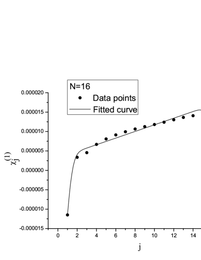
Figure 1: Plot of data points and the fitted curve of $\chi^{(1)}_{j}$ vs $j$ for $N=16$ and $\gamma=0.01$.

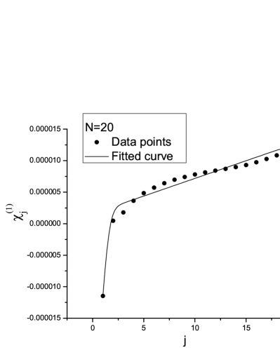
Figure 2: Plot of data points and the fitted curve of $\chi^{(1)}_{j}$ vs $j$ for $N=20$ and $\gamma=0.01$.

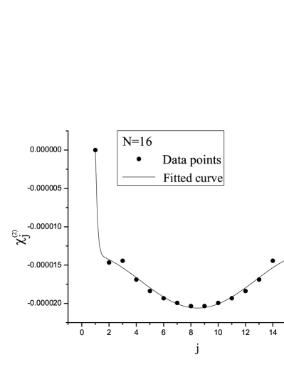
Figure 3: Plot of data points and the fitted curve of $\chi^{(2)}_{j}$ vs $j$ for $N=16$ and $\gamma=0.01$.

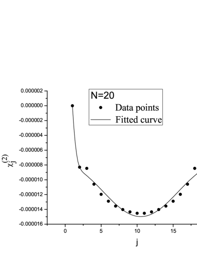
Figure 4: Plot of data points and the fitted curve of $\chi^{(2)}_{j}$ vs $j$ for $N=20$ and $\gamma=0.01$.

The obtained functional forms of $\chi^{(a)}_{j}$s ($a=1,2$) are as follows:

$$\chi^{(1)}_{j} = \frac{1+\eta_{1}j}{1+\eta_{1}}\Big{\{}\alpha_{1}(e^{-b_{1}}+e^{-b_{1}N^{2}}-e^{-b_{1}j^{2}}$$ (79)

$$-e^{-b_{1}(N+1-j)^{2}})+\chi^{(1)}_{1}\frac{e^{-b_{1}j^{2}}-e^{-b_{1}N^{2}}}{e^{-b_{1}}-e^{-b_{1}N^{2}}}\Big{\}},$$

$$\chi^{(2)}_{j} = \alpha_{2}\frac{1+\eta_{2}\sin^{2}j\nu}{1+\eta_{2}\sin^{2}\nu}\Big{\{}e^{-b_{2}j^{2}}+e^{-b_{2}(N+1-j)^{2}}-e^{-b_{2}}$$ (80)

$$-e^{-b_{2}N^{2}}\Big{\}},$$

where the property $\chi^{(2)}_{j}=\chi^{(2)}_{N+1-j}$ holds. We have shown in the next section that $\chi^{(1)}_{1}$ tends to a finite value in the thermodynamic limit. The value of the parameters for two different $N$ are given in the following two tables.

$N$	$\alpha_{1}$	$b_{1}$	$\eta_{1}$
$16$	$11.48\times 10^{-6}$	$1.05$	$0.27$
$20$	$5.16\times 10^{-6}$	$0.88$	$0.35$

Table 1: Parameters of $\chi^{(1)}_{j}$ for different $N$ and $\gamma=0.01$

$N$	$\alpha_{2}$	$b_{2}$	$\eta_{2}$
$16$	$43.53\times 10^{-5}$	$3.47$	$0.55$
$20$	$2.18\times 10^{-5}$	$0.96$	$0.83$

Table 2: Parameters of $\chi^{(2)}_{j}$ for different $N$ and $\gamma=0.01$

V Conduction current and Fourier’s law

The energy current density flown between ${\mathbf{n}}$ and ${\mathbf{n}}+\hat{e}_{1}$, where $\hat{e}_{1}=(1,0,0)$, reads as

$$j_{\mathbf{n}}=\frac{1}{2a^{2}}(\dot{x}_{{\mathbf{n}}+\hat{e}_{1}}+\dot{x}_{\mathbf{n}})\{C_{2}(x_{\mathbf{n}}-x_{{\mathbf{n}}+\hat{e}_{1}})+C_{4}(x_{\mathbf{n}}-x_{{\mathbf{n}}+\hat{e}_{1}})^{3}\}.$$ (81)

The average energy current density per bond along $n_{1}$ direction

$$J=\frac{1}{W_{2}W_{3}(N-1)}\sum_{{\mathbf{n}}_{\perp}}\sum_{n_{1}=1}^{N}j_{\mathbf{n}}=J_{1}+J_{2},$$ (82)

where

$$J_{1} = \frac{C_{2}}{2a^{2}W_{2}W_{3}(N-1)}\sum_{{\mathbf{n}}_{\perp}}\sum_{n_{1}=1}^{N}(\dot{x}_{{\mathbf{n}}+\hat{e}_{1}}+\dot{x}_{\mathbf{n}})$$ (83)

$$\times(x_{\mathbf{n}}-x_{{\mathbf{n}}+\hat{e}_{1}}),$$

$$J_{2} = \frac{C_{4}}{2a^{2}W_{2}W_{3}(N-1)}\sum_{{\mathbf{n}}_{\perp}}\sum_{n_{1}=1}^{N}(\dot{x}_{{\mathbf{n}}+\hat{e}_{1}}+\dot{x}_{\mathbf{n}})$$ (84)

$$\times(x_{\mathbf{n}}-x_{{\mathbf{n}}+\hat{e}_{1}})^{3}.$$

V.1 Calculation of $J_{1}$

We use the Fourier expansion of the the displacement fields from eq.(7) and also use eq.(18), (30), (36), (41) and (128) to obtain the expression of $J_{1}$ in eq.(83) to order $\lambda$ as

$$J_{1} = \frac{C_{2}}{2\pi a^{2}W_{2}W_{3}(N^{2}-1)}\sum_{\mathbf{q}}\sum_{k_{1},k_{2}=1}^{N}(1-(-1)^{k_{1}+k_{2}})$$ (85)

$$\times\sin k_{1}\nu\sin k_{2}\nu\int_{-\infty}^{\infty}\frac{d\omega}{2\pi}i\omega$$

$$\times\Big{[}\Big{(}1-\frac{1}{\cos k_{1}\nu-\cos k_{2}\nu}\Big{)}G^{(0)}_{k_{1}k_{2}}({\mathbf{q}},\omega)$$

$$-\frac{2}{\cos k_{1}\nu-\cos k_{2}\nu}G^{(1)}_{k_{1}k_{2}}({\mathbf{q}},\omega)+0(\lambda^{2})\Big{]}.$$

We first use eq.(37) and (42) and evaluate the frequency integrals using the results in eq.(107) and (109). Then using the results of appendix B we obtain the expression as

$$J_{1} = \frac{\gamma k_{B}T_{D}}{(N-1)a^{2}}\Big{[}\sum_{l=1}^{N}K^{(0)}_{l}\bar{z}_{l}+32\bar{\lambda}\sum_{l,l^{\prime}=1}^{N}K^{(1)}_{l,l^{\prime}}\bar{z}_{l}\bar{z}_{l^{\prime}}$$ (86)

$$+0(\bar{\lambda}^{2})\Big{]},$$

where the harmonic partShila2013

$$K^{(0)}_{l} = \frac{1}{(N+1)^{2}}\sum_{j,k=1}^{N}(1-(-1)^{j+k})\sin j\nu\sin k\nu$$ (87)

$$\times\sin(lj\nu)\sin(lk\nu)M^{(0)}_{jk}$$

and the anharmonic part

$$K^{(1)}_{l,l^{\prime}} = \frac{N}{(N+1)^{5}}\sum_{k_{1},k_{2},j_{1},j_{2},j_{3}=1}^{N}\sum_{s,s_{2},s_{3}=\pm}ss_{2}s_{3}$$ (88)

$$\times\sin k_{1}\nu\sin k_{2}\nu\sin(lj_{2}\nu)\sin(lj_{3}\nu)$$

$$\times\sin(l^{\prime}j_{1}\nu)\sin(l^{\prime}k_{1}\nu)\tilde{\delta}_{j_{1}+s_{2}j_{2}+s_{3}j_{3}+sk_{2}}$$

$$\times U(k_{1},k_{2},j_{1},j_{2},j_{3}).$$

The expression for $U(k_{1},k_{2},j_{1},j_{2},j_{3})$ reads as

$$U(k_{1},k_{2},j_{1},j_{2},j_{3})=\tilde{\gamma}^{2}(1-(-1)^{k_{1}+k_{2}})\Big{[}(g^{(2)}_{k_{1}k_{2}j_{1}}-\tilde{\gamma}^{2})$$

$$\times\Big{\{}g^{(1)}_{j_{1}j_{2}j_{3}k_{2}}M^{(2)}_{k_{1}k_{2}j_{1}}M^{(0)}_{j_{2}j_{3}}+\frac{1}{2}M^{(3)}_{k_{1}k_{2}j_{1}}M^{(1)}_{j_{2}j_{3}}\Big{\}}$$

$$-\frac{1}{\cos k_{1}\nu-\cos k_{2}\nu}\Big{\{}g^{(1)}_{j_{1}j_{2}j_{3}k_{2}}M^{(0)}_{k_{1}j_{1}}M^{(0)}_{j_{2}j_{3}}$$

$$+\frac{1}{2}M^{(1)}_{k_{1}j_{1}}M^{(1)}_{j_{2}j_{3}}\Big{\}}\Big{]}$$ (89)

Although there is a factor of $\cos k_{1}\nu-\cos k_{2}\nu$ in the denominator of the second term of $U(k_{1},k_{2},j_{1},j_{2},j_{3})$, owing to the following result that

$$\lim_{k_{1}\rightarrow k_{2}}\frac{(1-(-1)^{k_{1}+k_{2}})}{\cos k_{1}\nu-\cos k_{2}\nu}=0,$$ (90)

it remains finite and goes to zero in the limit when $k_{1}$ goes to $k_{2}$.

V.2 Calculation of $J_{2}$

We obtain the expression of $J_{2}$ to order $\lambda$ after using eq.(7), (18), (30), (36) and (LABEL:dsum2) in eq.(84) as

$$J_{2} = \frac{3m\omega_{h}^{2}\lambda}{32\pi^{2}a^{4}(W_{2}W_{3})^{2}(N-1)}\sum_{k_{1},k_{2},k_{3},k_{4}=1}^{N}$$ (91)

$$\times{\cal N}(k_{1},k_{2},k_{3},k_{4})\sum_{{\mathbf{q}},{\mathbf{q}}^{\prime}}\int_{-\infty}^{\infty}\frac{d\omega}{2\pi}\frac{d\omega^{\prime}}{2\pi}i\omega G^{(0)}_{k_{1}k_{2}}({\mathbf{q}},\omega)$$

$$\times G^{(0)}_{k_{3}k_{4}}({\mathbf{q}}^{\prime},\omega^{\prime})+0(\lambda^{2}),$$

where we have used the symmetry properties of ${\cal N}(k_{1},k_{2},k_{3},k_{4})$ given in eqn.(131). We carry out the frequency integrations using eq.(105) and (107) and then use the results of appendix B to arrive at the expression

$$J_{2}=\frac{48\bar{\lambda}\gamma k_{B}T_{D}}{(N-1)a^{2}}\sum_{l,l^{\prime}=1}^{N}K^{(2)}_{l,l^{\prime}}\bar{z}_{l}\bar{z}_{l^{\prime}}+0(\bar{\lambda}^{2}),$$ (92)

where

$$K^{(2)}_{l,l^{\prime}} = -\frac{\tilde{\gamma}^{2}}{(N+1)^{4}}\sum_{k_{1},k_{2},k_{3},k_{4}=1}^{N}\{1-(-1)^{k_{1}+k_{2}+k_{3}+k_{4}}\}$$

$$\times{\cal N}_{1}(k_{1},k_{2},k_{3},k_{4})(\cos k_{1}\nu-\cos k_{2}\nu)M^{(0)}_{k_{1}k_{2}}$$

$$\times M^{(0)}_{k_{3}k_{4}}\sin(lk_{1}\nu)\sin(lk_{2}\nu)\sin(l^{\prime}k_{3}\nu)\sin(l^{\prime}k_{4}\nu).$$

The expression for ${\cal N}_{1}(k_{1},k_{2},k_{3},k_{4})$ is given in eq.(130).

V.3 Thermal conductivity

The final expression according to eq.(86) and (92) for average energy current density per bond reads as

$$J = \frac{\gamma k_{B}T_{D}}{(N-1)a^{2}}\Big{[}\sum_{l=1}^{N}K^{(0)}_{l}\bar{z}_{l}+16\bar{\lambda}\sum_{l,l^{\prime}=1}^{N}(2\,K^{(1)}_{l,l^{\prime}}$$ (94)

$$3\,K^{(2)}_{l,l^{\prime}})\bar{z}_{l}\bar{z}_{l^{\prime}}+0(\bar{\lambda}^{2})\Big{]}.$$

It is evident from the expressions given in eq.(87), (88) and (LABEL:K2) for $K^{(0)}$, $K^{(1)}_{l,l^{\prime}}$ and $K^{(2)}_{l,l^{\prime}}$ respectively that the following properties hold for them.

$$K^{(0)}_{l} = -K^{(0)}_{N+1-l},$$ (95)

$$K^{(1)}_{l,l^{\prime}} = -K^{(1)}_{N+1-l,N+1-l^{\prime}},$$ (96)

$$K^{(2)}_{l,l^{\prime}} = -K^{(1)}_{N+1-l,N+1-l^{\prime}}.$$ (97)

We then use these properties and eq.(63) in eq.(94) to obtain

$$J = \frac{\gamma k_{B}T_{D}}{(N-1)a^{2}}(\bar{z}_{1}-\bar{T}_{e})\Big{[}K^{(0)}_{1}+16\bar{\lambda}\Big{\{}\bar{T}_{e}\sum_{l=2}^{N/2}\{2(K^{(1)}_{1,l}$$

$$+K^{(1)}_{l,1}-K^{(1)}_{N,l}-K^{(1)}_{l,N})+3(K^{(2)}_{1,l}+K^{(2)}_{l,1}-K^{(2)}_{N,l}$$

$$-K^{(2)}_{l,N})\}+(\bar{z}_{1}+\bar{T}_{e})(2\,K^{(1)}_{1,1}+3\,K^{(2)}_{1,1})\Big{\}}+0(\bar{\lambda}^{2})\Big{]},$$

where we have assumed $N$ as even. Then after using eq.(70) we obtain the average energy current density per bond as

$$J=\kappa\frac{T_{1}-T_{N}}{(N-1)a},$$ (99)

where the thermal conductivity to order $\bar{\lambda}$ reads as

$$\kappa = \frac{\gamma k_{B}}{2a(C^{(0)}_{1,1}-C^{(0)}_{N,1})}\Big{[}K^{(0)}_{1}$$

$$+16\bar{\lambda}\Big{\{}\bar{T}_{e}\Big{(}\chi^{(4)}-\frac{2K_{1}^{(0)}\chi^{(2)}_{1}}{C^{(0)}_{1,1}-C^{(0)}_{N,1}}\Big{)}$$

$$+\frac{\bar{T}_{1}-\bar{T}_{N}}{2(C^{(0)}_{1,1}-C^{(0)}_{N,1})}\Big{(}\chi^{(3)}-\frac{2K_{1}^{(0)}\chi^{(1)}_{1}}{C^{(0)}_{1,1}-C^{(0)}_{N,1}}\Big{)}\Big{\}}+0(\bar{\lambda}^{2})\Big{]}.$$

The expressions for $\chi^{(3)}$ and $\chi^{(4)}$ are given in the following:

$$\chi^{(3)} = 2K^{(1)}_{1,1}+3K^{(2)}_{1,1}$$ (101)

$${\rm and}~{}~{}\chi^{(4)} = \sum_{l=1}^{N-1}\{2(K^{(1)}_{1,l}+K^{(1)}_{l,1})+3(K^{(2)}_{1,l}+K^{(2)}_{l,1})\}.$$

We have evaluated $\chi^{(1)}_{1}$, $\chi^{(2)}_{1}$, $\chi^{(3)}$, $\chi^{(4)}$ and $K^{(0)}_{1}$ numerically for different $N$ and taking $\gamma=0.01$. Our evaluations give $\chi^{(2)}=0.0$ and $\chi^{(4)}=0.0$ for all $N$ and $K^{(0)}\rightarrow 18.09$ in the thermodynamic limit. The remaining results are given in the following table.

$N$	$\chi^{(1)}_{1}$	$\chi^{(3)}$
$10$	$-1.08\times 10^{-5}$	$-3.25\times 10^{-2}$
$16$	$-1.15\times 10^{-5}$	$-3.63\times 10^{-2}$
$20$	$-1.15\times 10^{-5}$	$-3.66\times 10^{-2}$
$24$	$-1.13\times 10^{-5}$	$-3.6\times 10^{-2}$
$30$	$-1.09\times 10^{-5}$	$-3.41\times 10^{-2}$
$34$	$-1.05\times 10^{-5}$	$-3.26\times 10^{-2}$
$40$	$-1.01\times 10^{-5}$	$-3.01\times 10^{-2}$

Table 3: $\chi^{(1)}_{1}$ and $\chi^{(3)}_{1}$ for different $N$ and $\gamma=0.01$

It is clear that owing to vanishing values of $\chi^{(2)}_{1}$ and $\chi^{(4)}$ for any $N$, $\kappa$ remains insensitive to the environment temperature $T_{e}$ to order $\bar{\lambda}$. Since $\chi^{(1)}_{1}\rightarrow 10^{-5}$, and $\chi^{(3)}\rightarrow 3\times 10^{-2}$ in the thermodynamic limit, $\kappa$ receives a finite, non zero and temperature dependent contribution which is linearly proportional to $T_{1}-T_{N}$ at its $\bar{\lambda}$ order. Thus $\kappa$ remains finite in the thermodynamic limit and hence Fourier’s law holds to order $\bar{\lambda}$.

VI Summary

We have taken an ordered, anharmonic, three dimensional crystal in the form of a slab geometry. We have attached Langevin type baths to the first and the $N$-th surfaces along its length maintaining the fixed temperatures $T_{1}$ and $T_{N}$ respectively. In order to simulate the environment surrounding the crystal, we have attached heat baths of same type to the remaining $N-2$ surfaces of the slab. We have chosen the noise functions of $N$ baths Gaussian and their widths $z_{j}$ ($1\leq j\leq N$) as site dependent. In the steady state, when $t\gg\frac{1}{\gamma}$, each surface behaves as a thermally equilibriated system and the slab as a whole behaves as an assembly of $N$ such systems at different temperatures. Our evaluation have shown that the average radiated energy per unit time from a particle in any one of the $N$ surfaces does not receive any correction at the order $\bar{\lambda}$. We have taken $z_{j}$ as proportional to the environment temperature $T_{e}$ for $2\leq j\leq N$ and have found that the radiated energies from $N-1$ layers obey Newton’s law of cooling. We have shown that the exponentially falling nature from high to low temperature end of the slab is the leading behaviour of the temperature profile. The non-leading behaviour of the profile at the order $\bar{\lambda}$ is governed by the two functions $\chi^{(1)}_{j}$ and $\chi^{(2)}_{j}$. Our numerical evaluations have shown that the thermal conductivity $\kappa$ remains independent of the environment temperature $T_{e}$ but it is dependent linearly on $T_{1}-T_{N}$ at the order $\bar{\lambda}$. Moreover, since $\kappa$ remains finite in the thermodynamic limit, Fourier’s law holds to order $\bar{\lambda}$.

Appendix A Frequency Integrals

Consider the integral

$${\cal I}^{(1)}_{j}({\mathbf{q}}) = \int^{\infty}_{-\infty}\frac{d\omega}{2\pi}\omega D_{j}({\mathbf{q}},\omega)$$ (103)

$$= -\int^{\infty}_{-\infty}\frac{d\omega}{2\pi}\frac{\omega}{\omega^{2}-\omega^{2}_{j}({\mathbf{q}})-i\gamma\omega}.$$

To evaluate this integral we consider the complex $\omega$ plane and choose a closed, semi circular contour which is closed in the upper half of the complex plane. Since the contour encloses the poles at $\pm\sqrt{\omega^{2}_{k}({\mathbf{q}})-\frac{\gamma^{2}}{4}}+i\frac{\gamma}{2}$ the result of our evaluation is

$${\cal I}^{(1)}_{j}({\mathbf{q}})=-i$$ (104)

Integrals of the following types are evaluated in the similar manner and results are quoted below.

$${\cal I}^{(2)}_{jk}({\mathbf{q}})=\int^{\infty}_{\infty}\frac{d\omega}{2\pi}D_{j}({\mathbf{q}},\omega)D_{k}(-{\mathbf{q}},-\omega)=\frac{2\gamma}{B_{jk}(\mathbf{q})},$$ (105)

where

$$B_{jk}({\mathbf{q}})=(\omega^{2}_{j}({\mathbf{q}})-\omega^{2}_{k}({\mathbf{q}}))^{2}+2\gamma^{2}(\omega^{2}_{j}({\mathbf{q}})+\omega^{2}_{k}({\mathbf{q}})).$$ (106)

$${\cal I}^{(3)}_{jk}({\mathbf{q}}) = \int^{\infty}_{-\infty}\frac{d\omega}{2\pi}\omega D_{j}({\mathbf{q}},\omega)D_{k}(-{\mathbf{q}},-\omega)$$ (107)

$$= \frac{i(\omega^{2}_{j}({\mathbf{q}})-\omega^{2}_{k}({\mathbf{q}}))}{B_{jk}(\mathbf{q})}.$$

$${\cal I}^{(4)}_{jk}({\mathbf{q}}) = \int^{\infty}_{-\infty}\frac{d\omega}{2\pi}\omega^{2}D_{j}({\mathbf{q}},\omega)D_{k}(-{\mathbf{q}},-\omega)$$ (108)

$$= \frac{\gamma(\omega^{2}_{j}({\mathbf{q}})+\omega^{2}_{k}({\mathbf{q}}))}{B_{jk}(\mathbf{q})}.$$

$${\cal I}^{(5)}_{jkl}({\mathbf{q}}) = \int^{\infty}_{-\infty}\frac{d\omega}{2\pi}\omega D_{j}({\mathbf{q}},\omega)D_{k}(-{\mathbf{q}},-\omega)D_{l}(-{\mathbf{q}},-\omega)$$ (109)

$$= \frac{-i}{B_{jk}({\mathbf{q}})B_{jl}({\mathbf{q}})}$$

$$\times\{(\omega^{2}_{j}({\mathbf{q}})-\omega^{2}_{k}({\mathbf{q}}))(\omega^{2}_{j}({\mathbf{q}})-\omega^{2}_{l}({\mathbf{q}}))$$

$$-4\gamma^{2}\omega^{2}_{j}({\mathbf{q}})\}.$$

$${\cal I}^{(6)}_{jkl}({\mathbf{q}}) = \int^{\infty}_{-\infty}\frac{d\omega}{2\pi}\omega^{2}D_{j}({\mathbf{q}},\omega)D_{k}(-{\mathbf{q}},-\omega)D_{l}(-{\mathbf{q}},-\omega)$$ (110)

$$= \frac{-\gamma}{B_{jk}({\mathbf{q}})B_{jl}({\mathbf{q}})}$$

$$\times\{(\omega^{2}_{j}({\mathbf{q}})+\omega^{2}_{l}({\mathbf{q}}))(\omega^{2}_{j}({\mathbf{q}})-\omega^{2}_{k}({\mathbf{q}}))$$

$$+2\omega^{2}_{j}(\omega^{2}_{j}({\mathbf{q}})-\omega^{2}_{l}({\mathbf{q}}))\}.$$

$${\cal I}^{(7)}_{jk}({\mathbf{q}})=\int^{\infty}_{-\infty}\frac{d\omega}{2\pi}\omega D_{j}({\mathbf{q}},\omega)D_{k}({\mathbf{q}},\omega)=0.$$ (111)

Appendix B Wave vector sums in the continuum limit

Consider the sum

$${\cal M}^{(0)}_{jk}=\frac{1}{W_{2}W_{3}}\sum_{\mathbf{q}}\frac{1}{B_{jk}(\mathbf{q})}$$ (112)

In the continuum limit ,

$$\frac{1}{W_{2}W_{3}}\sum_{\mathbf{q}}\rightarrow\frac{a^{2}}{(2\pi)^{2}}\int^{\frac{\pi}{a}}_{-\frac{\pi}{a}}\int^{\frac{\pi}{a}}_{-\frac{\pi}{a}}dq_{2}dq_{3}$$ (113)

and

$${\cal M}^{(0)}_{jk}=\frac{16}{\pi^{2}\omega^{4}_{h}}\int^{\frac{\pi}{2}}_{0}\int^{\frac{\pi}{2}}_{0}\frac{d\theta_{2}\theta_{3}}{e_{jk}(\theta_{2},\theta_{3})},$$ (114)

where $\tilde{\gamma}=\frac{2\gamma}{\omega_{h}}$ and

$$e_{jk}(\theta_{2},\theta_{3})=E_{jk}+4{\tilde{\gamma}}^{2}(\sin^{2}\theta_{2}+\sin^{2}\theta_{3}).$$ (115)

$E_{jk}$ is given as

$$E_{jk}=(\cos j\nu-\cos k\nu)^{2}+\tilde{\gamma}^{2}(\cos j\nu+\cos k\nu+2).$$ (116)

We have evaluated the double integrals and expressed the result in terms of hypergeometric function as

$${\cal M}^{(0)}_{jk}=\frac{4}{\omega^{4}_{h}}M^{(0)}_{jk},$$ (117)

where

$$M^{(0)}_{jk} = \frac{1}{\Delta_{jk}}F(\frac{1}{2},\frac{1}{2},1;(\frac{4\tilde{\gamma}^{2}}{\Delta_{jk}})^{2}),$$ (118)

$$\Delta_{jk} = (\cos j\nu-\cos k\nu)^{2}$$ (119)

$$+\tilde{\gamma}^{2}(\cos j\nu+\cos k\nu+6).$$

In a similar manner the following sums can also be expressed in terms of integrals in the continuum limit:

$${\cal M}^{(1)}_{jk} = \frac{1}{W_{2}W_{3}}\sum_{\mathbf{q}}\frac{\sin^{2}{(\frac{q_{2}a}{2})}}{B_{jk}(\mathbf{q})}=\frac{1}{W_{2}W_{3}}\sum_{\mathbf{q}}\frac{\sin^{2}{(\frac{q_{3}a}{2})}}{B_{jk}(\mathbf{q})}$$ (120)

$$= \frac{1}{8\gamma^{2}\omega^{2}_{h}}(1-E_{jk}M^{(0)}_{jk}),$$

$${\cal M}^{(2)}_{jkl} = \frac{1}{W_{2}W_{3}}\sum_{\mathbf{q}}\frac{1}{B_{jk}(\mathbf{q})B_{jl}(\mathbf{q})}$$ (121)

$$= \frac{16}{\omega^{8}_{h}}\frac{M^{(0)}_{jk}-M^{(0)}_{jl}}{E_{jl}-E_{jk}},$$

The following sums over wave vector are decomposed in terms of $M^{(0)}_{jk}$:

$$\frac{1}{W_{2}W_{3}}\sum_{\mathbf{q}}\frac{\sin^{2}{\frac{q_{2}a}{2}}+\sin^{2}{\frac{q_{3}a}{2}}}{B_{jk}(\mathbf{q})B_{jl}(\mathbf{q})}$$

$$= \frac{1}{\gamma^{2}\omega^{6}_{h}}\frac{E_{jl}M^{(0)}_{jl}-E_{jk}M^{(0)}_{jk}}{E_{jl}-E_{jk}},$$

$$\frac{1}{W_{2}W_{3}}\sum_{\mathbf{q}}\frac{(\sin^{2}{\frac{q_{2}a}{2}}+\sin^{2}{\frac{q_{3}a}{2}})^{2}}{B_{jk}(\mathbf{q})B_{jl}(\mathbf{q})}$$

$$= \frac{1}{16\gamma^{4}\omega_{h}^{4}}\frac{E_{jl}-E_{jk}+E^{2}_{jk}M^{(0)}_{jk}-E^{2}_{jl}M^{(0)}_{jl}}{E_{jl}-E_{jk}}.$$ (123)

Appendix C Definition of useful integrals

$$M^{(1)}_{jk} = \frac{4}{\pi^{2}}\int_{0}^{\frac{\pi}{2}}\int_{0}^{\frac{\pi}{2}}d\theta_{2}d\theta_{3}\frac{\sin^{2}\theta_{2}+\sin^{2}\theta_{3}}{e_{jk}(\theta_{2},\theta_{3})},$$ (124)

$$M^{(2)}_{jkl} = \frac{4}{\pi^{2}}\int_{0}^{\frac{\pi}{2}}\int_{0}^{\frac{\pi}{2}}d\theta_{2}d\theta_{3}\frac{1}{e_{jk}(\theta_{2},\theta_{3})e_{jl}(\theta_{2},\theta_{3})},$$ (125)

$$M^{(3)}_{jkl} = \frac{4}{\pi^{2}}\int_{0}^{\frac{\pi}{2}}\int_{0}^{\frac{\pi}{2}}d\theta_{2}d\theta_{3}\frac{\sin^{2}\theta_{2}+\sin^{2}\theta_{3}}{e_{jk}(\theta_{2},\theta_{3})e_{jl}(\theta_{2},\theta_{3})},$$ (126)

$$M^{(4)}_{jkl} = \frac{4}{\pi^{2}}\int_{0}^{\frac{\pi}{2}}\int_{0}^{\frac{\pi}{2}}d\theta_{2}d\theta_{3}\frac{(\sin^{2}\theta_{2}+\sin^{2}\theta_{3})^{2}}{e_{jk}(\theta_{2},\theta_{3})e_{jl}(\theta_{2},\theta_{3})}.$$ (127)

Appendix D Discrete sums

$$\sum_{n_{1}=1}^{N-1}(A_{n_{1},j}+A_{n_{1}+1,j})(A_{n_{1},k}-A_{n_{1}+1,k})$$ (128)

$$= \frac{2}{N+1}(1-(-1)^{j+k})\sin j\nu\sin k\nu$$

$$\times\Big{(}1-\frac{1}{\cos j\nu-\cos k\nu}\Big{)}.$$

$${\cal N}(k_{1},k_{2},k_{3},k_{4})$$

$$= \sum_{n_{1}=1}^{N-1}(A_{n_{1},k_{1}}+A_{n_{1}+1,k_{1}})(A_{n_{1},k_{2}}-A_{n_{1}+1,k_{2}})$$

$$\times(A_{n_{1},k_{3}}-A_{n_{1}+1,k_{3}})(A_{n_{1},k_{4}}-A_{n_{1}+1,k_{4}})$$

$$= \frac{8}{(N+1)^{2}}\{1-(-1)^{k_{1}+k_{2}+k_{3}+k_{4}}\}{\cal N}_{1}(k_{1},k_{2},k_{3},k_{4}),$$

where

$${\cal N}_{1}(k_{1},k_{2},k_{3},k_{4}) = \sin k_{1}\nu\cos\frac{k_{2}\nu}{2}\cos\frac{k_{3}\nu}{2}\cos\frac{k_{4}\nu}{2}$$ (130)

$$\times\Big{[}4\sin\frac{k_{2}\nu}{2}\sin\frac{k_{3}\nu}{2}\sin\frac{k_{4}\nu}{2}$$

$$+\frac{\sin\frac{(k_{2}-k_{3}+k_{4})\nu}{2}}{\cos(k_{2}-k_{3}+k_{4})\nu-\cos k_{1}\nu}$$

$$+\frac{\sin\frac{(k_{2}+k_{3}-k_{4})\nu}{2}}{\cos(k_{2}+k_{3}-k_{4})\nu-\cos k_{1}\nu}$$

$$-\frac{\sin\frac{(k_{2}-k_{3}-k_{4})\nu}{2}}{\cos(k_{2}-k_{3}-k_{4})\nu-\cos k_{1}\nu}$$

$$-\frac{\sin\frac{(k_{2}+k_{3}+k_{4})\nu}{2}}{\cos(k_{2}+k_{3}+k_{4})\nu-\cos k_{1}\nu}\Big{]}.$$

${\cal N}(k_{1},k_{2},k_{3},k_{4})$ has the following symmetries:

$${\cal N}(k_{1},k_{2},k_{3},k_{4}) = {\cal N}(k_{1},k_{3},k_{2},k_{4})={\cal N}(k_{1},k_{4},k_{3},k_{2})$$ (131)

$$= {\cal N}(k_{1},k_{2},k_{4},k_{3}).$$

References

- (1) M. N. Saha and B. N. Srivastava, A Treatise on Heat, 5th edition (The Indian Press, Allahabad, 1969), p. 462 - 465.
- (2) F.Bonetto, J. L. Lebowitz, and L. Rey-Bellet, Mathematical Physics 2000, edited by A. Fokas, A. Grigoryan, T. Kibble and B. Zegarlinski (Imperial College Press, London, 2000), p. 128 – 150.
- (3) S. Lepri, R. Livi, and A. Politi, Phys. Rep. , 1(2003).
- (4) P. M. Chaikin and T. C. Lubensky, Principles of condensed matter physics (Cambridge University Press, New Delhi, 2009).
- (5) F. Reif, Fundamentals of Statistical and Thermal Physics (McGraw-Hill, Singapore, 1985).
- (6) Z. Rieder, J. L. Lebowitz, and E. Lieb, J. Math. Phys. , 1073(1967).
- (7) H. Nakazawa, Prog. Theor. Phys. Suppl. , 231(1970).
- (8) R. Rubin and W. Greer, J. Math. Phys. (N.Y.) , 1686(1971).
- (9) A. J. O’Connor and J. L. Lebowitz, J. Math. Phys. , 692(1974).
- (10) A. Dhar, Phys. Rev. Lett. , 5882(2001).
- (11) L. W. Lee and A. Dhar, Phys. Rev. Lett. , 094302(2005).
- (12) A. Chaudhuri, A. Kundu, D. Roy, A. Dhar, J. L. Lebowitz, and H. Spohn, Phys. Rev. , 064301(2010).
- (13) K. Saito and A. Dhar, Phys. Rev. Lett. , 040601(2010).
- (14) M. Bolsterli, M. Rich, and W. M. Visscher, Phys. Rev. , 1086(1970).
- (15) M. Rich and W. M. Visscher, Phys. Rev. , 2164(1975).
- (16) F. Bonetto, J. L. Lebowitz, and J. Lukkarinen, J. Stat. Phys. , 783(2004).
- (17) S.Acharya and K. Mukherjee, Int. J. Mod. Phys. , 1350057(2013); erratum: , 1392003(2013).