A diabatic definition of geometric phase effects

Abstract

Electronic wave-functions in the adiabatic representation acquire nontrivial geometric phases (GPs) when corresponding potential energy surfaces undergo conical intersection (CI). These GPs have profound effects on the nuclear quantum dynamics and cannot be eliminated in the adiabatic representation without changing the physics of the system. To define dynamical effects arising from the GP presence the nuclear quantum dynamics of the CI containing system is compared with that of the system with artificially removed GP. We explore a new construction of the system with removed GP via a modification of the diabatic representation for the original CI containing system. Using an absolute value function of diabatic couplings we remove the GP while preserving adiabatic potential energy surfaces and CI. We assess GP effects in dynamics of a two-dimensional linear vibronic coupling model both for ground and excited state dynamics. Results are compared with those obtained with a conventional removal of the GP by ignoring double-valued boundary conditions of the real electronic wave-functions. Interestingly, GP effects appear similar in two approaches only for the low energy dynamics. In contrast with the conventional approach, a new approach does not have substantial GP effects in the ultra-fast excited state dynamics.

I Introduction

Ubiquitous in molecules beyond diatomics, conical intersections (CIs) of electronic states act as “funnels” Balzer, Hahn, and Stock (2003); Köppel, Domcke, and Cederbaum (1984); Yarkony (1996); Hahn and Stock (2000) that enable rapid conversion of the excessive electronic energy into nuclear motion. Also, CIs lead to the appearance of the geometric phase (GP) Berry (1984); Mead and Truhlar (1979); Berry (1987) in both electronic and nuclear wave-functions of the adiabatic representation. The GP presence leads to a sign change of adiabatic electronic wave-functions along a closed path of nuclear configurations encircling the CI seam.Longuet-Higgins et al. (1958); Mead and Truhlar (1979) This sign change affects evaluation of nonadiabatic couplings (NACs) necessary to complete the nuclear kinetic energy part of the adiabatic representation to define a nuclear Schrödinger equation. Changes in NACs due to the GP can lead to profound modification of nuclear dynamics even in situations when the nuclear wave-function is localized far from the region of CI. For example, the GP causes an extra phase accumulation for fragments of the nuclear wave-packet that move around the CI on opposite sides.Schön and Köppel (1995); Ryabinkin and Izmaylov (2013) This leads to destructive interference that gives rise either to a spontaneous localization of the nuclear density Ryabinkin and Izmaylov (2013) or slower nuclear dynamics Joubert-Doriol, Ryabinkin, and Izmaylov (2013) than in the case where the GP is neglected.

To distinguish unambiguously what is the effect of the GP on the nuclear dynamics one can study the exact quantum dynamics, which necessarily incorporates all GP effects, in comparison with the dynamics that is not including the GP. This comparison would allow one to formulate unique dynamical features related to the CI topology which gives rise to the GP. A natural question is how to modify a computational scheme to remove the GP with a minimal effect on other parts of dynamics? Previously, to analyze GP effects constructing a GP excluded version has been done by switching to the adiabatic representation.Hazra, Balakrishnan, and Kendrick (2015); Kendrick and Pack (1996); Kendrick (2003); Althorpe, Stecher, and Bouakline (2008); Baer (2000) A straightforward simulation of the nuclear dynamics ignoring double-valued character of electronic and nuclear wave-functions in the adiabatic representation excludes the GP.Mead and Truhlar (1979) As shown by Mead and Truhlar, the only change that is needed to obtain the correct nuclear dynamics in the adiabatic representation is a phase modification for both electronic and nuclear wave-functions that returns single-valued boundary conditions to these functions.Mead and Truhlar (1979) This phase change modifies only the kinetic energy terms, NACs, in the nuclear Hamiltonian and leaves potential energy terms unchanged. A practical difficulty with this approach is that it requires performing quantum nuclear dynamics in the adiabatic representation where many NAC components diverge at the CI. The necessity to work in the adiabatic representation creates technical challenges for investigation of GP effects in realistic systems beyond low dimensional simple models.

In this paper we propose an alternative way of investigating GP effects by introducing a modification in the system diabatic Hamiltonian, this modification removes the GP in the corresponding adiabatic representation without altering potential energy surfaces. Our modification is not equivalent to ignoring double-valued boundary conditions in the adiabatic representation and provides a new set of results characterizing GP effects in CI problems.

The rest of the paper is organized as follows. In Sec. II we introduce our approach for a two-dimensional linear vibronic coupling model problem with CI. Section III provides numerical results comparing GP effects obtained in the new diabatic and old adiabatic approaches on a set of model systems parametrized using real molecular systems. Finally, Sec. IV concludes the work by summarizing main results.

II Theoretical analysis

We introduce two models within the two-dimensional linear vibronic coupling (LVC) Hamiltonian

$$\hat{H}_{\rm LVC}={\hat{T}}{\mathbf{1}}_{2}+\begin{pmatrix}V_{11}&V_{12}\\ V_{12}&V_{22}\end{pmatrix},$$ (1)

where $\hat{T}=-\frac{1}{2}\nabla^{2}\equiv-\frac{1}{2}(\partial^{2}/\partial x^{2}+\partial^{2}/\partial y^{2})$ is the nuclear kinetic energy operator, and ${\mathbf{1}}_{2}$ is a $2\times 2$ unit matrix. $V_{11}$ and $V_{22}$ are the diabatic potentials represented by identical 2D parabolas shifted in the $x$-direction by $a$ and in energy by $\Delta$

$$V_{11}={} \frac{\omega_{1}^{2}}{2}x^{2}+\frac{\omega_{2}^{2}}{2}y^{2},$$ (2)

$$V_{22}={} \frac{\omega_{1}^{2}}{2}\left(x-a\right)^{2}+\frac{\omega_{2}^{2}}{2}y^{2}-\Delta.$$ (3)

To have the CI in the adiabatic representation, $V_{11}$ and $V_{22}$ are coupled by a linear potential $V_{12}=cy$ in model 1 and by an absolute value of a linear potential $V_{12}=c|y|$ in model 2.

Switching to the adiabatic representation for the 2D LVC Hamiltonian in Eq. (1) is done by diagonalizing the potential matrix using a unitary transformation

$$U=\begin{pmatrix}\cos\theta&\sin\theta\\ -\sin\theta&\cos\theta\end{pmatrix}$$ (4)

that introduces adiabatic electronic states

$$\ket{\phi_{1}^{\text{adi}}} = \phantom{-}\cos\theta\,\ket{\phi_{1}}+\sin\theta\,\ket{\phi_{2}},$$ (5)

$$\ket{\phi_{2}^{\text{adi}}} = -\sin\theta\,\ket{\phi_{1}}+\cos\theta\,\ket{\phi_{2}},$$ (6)

with $\theta=\theta(x,y)$ as a rotation angle between the diabatic electronic states $\ket{1}$ and $\ket{2}$

$$\theta=\frac{1}{2}\arctan\dfrac{2\,V_{12}}{V_{22}-V_{11}}.$$ (7)

The transformation in Eq. (4) gives rise to the 2D LVC Hamiltonian in the adiabatic representation $\hat{H}_{\text{adi}}=U^{\dagger}{\hat{H}}_{\rm LVC}U$,

$$\hat{H}_{\text{adi}}=\begin{pmatrix}\hat{T}+\hat{\tau}_{11}&\hat{\tau}_{12}\\ \hat{\tau}_{21}&\hat{T}+\hat{\tau}_{22}\end{pmatrix}+\begin{pmatrix}W_{-}&0\\ 0&W_{+}\end{pmatrix},$$ (8)

where

$$W_{\pm}= {}\dfrac{1}{2}\left(V_{11}+V_{22}\right)\pm\dfrac{1}{2}\sqrt{\left(V_{11}-V_{22}\right)^{2}+4V_{12}^{2}}$$ (9)

are the adiabatic potentials which are exactly the same for models 1 and 2, and $\hat{\tau}_{ij}=-\bra{\phi_{i}^{\text{adi}}}\nabla\phi_{j}^{\text{adi}}\rangle\nabla-\bra{\phi_{i}^{\text{adi}}}\nabla^{2}\phi_{j}^{\text{adi}}\rangle/2$ are the nonadiabatic couplings. For two-electronic-state models we can express $\hat{\tau}_{ij}$ as

$$\hat{\tau}_{11} {}=\hat{\tau}_{22}=\frac{1}{2}\nabla\theta\cdot\nabla\theta$$ (10)

$$\hat{\tau}_{12} {}=-\hat{\tau}_{21}=\frac{1}{2}\left(\nabla^{2}\theta+2\nabla\theta\cdot\nabla\right).$$ (11)

The diagonal non-adiabatic couplings, $\hat{\tau}_{11}$ and $\hat{\tau}_{22}$, represent a repulsive potential known as the diagonal Born–Oppenheimer correction (DBOC).Born and Huang (1954); Handy and Lee (1996); Valeev and Sherrill (2003) The off-diagonal elements, $\hat{\tau}_{12}$ and $\hat{\tau}_{21}$ in Eq. (11), couple dynamics on the adiabatic potentials $W_{\pm}$ and are responsible for non-adiabatic transitions. All $\hat{\tau}_{ij}$ terms involve derivative of $\theta$ which is given by two different functions

$$\theta_{1} = \frac{1}{2}\arctan\dfrac{\gamma y}{x-b},$$ (12)

$$\theta_{2} = \frac{1}{2}\arctan\dfrac{\gamma|y|}{x-b}$$ (13)

for models 1 and 2, respectively. Here, $b=\Delta/(\omega_{1}^{2}a)$ is the $x$-coordinate of the CI point, and $\gamma={2c}/{(\omega_{1}^{2}a)}$ is dimensionless coupling strength. For simplicity of the subsequent analysis we set $b=0$, which corresponds to centring the coordinates at the CI point. To see the difference between $\theta_{1}$ and $\theta_{2}$ we will continuously track their changes along a contour encircling the CI. For the CI located at the origin we have taken a set of points on a circle $(x_{j},y_{j})$ parametrized by the polar representation of complex numbers $x_{j}+iy_{j}=re^{i\phi_{j}}$, where $r=1$ and $\phi_{j}$’s are taken from the discretized $[0,2\pi]$ interval. Figure 1 illustrates that $\theta_{1}$ changes by $\pi$ when we do the full circle while $\theta_{2}$ returns to its initial value, 0.

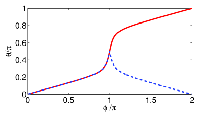
Figure 1: $\theta$ angle of the diabatic-to-adiabatic transformation as a function of the CI encircling angle $\phi$ for two models: red solid for model 1 [Eq. (12)] and blue dashed for model 2 [Eq. (13)].

For the adiabatic electronic functions [Eqs. (5)-(6)] this means that these functions change their signs in model 1 and return to their original values in model 2. Therefore, models 1 and 2 have electronic functions which are double- and single-valued functions of nuclear parameters, respectively. In terms of differentiability, $\theta_{2}$ clearly has issues at the $y=0$ line. However, we will not compute $\hat{\tau}_{ij}$ elements for model 2 because all simulations for this model will be done in the diabatic representation.

Another possible concern for our approach could be that the modification of the diabatic model removing the GP breaks smoothness of the diabatic coupling as a function of the nuclear coordinate. This raises a question of the physical meaning of the diabatic model with such a coupling term. It is important to understand that the GP is a significant part of the CI topology and removing it in any way is expected to produce an incomplete and thus in some sense unphysical picture. To illustrate this point even further we will show that the diabatic model which is mathematically equivalent to the adiabatic model with the GP removed in the conventional way has divergent diabatic potentials with discontinuous derivatives. First, let us clarify that to obtain the adiabatic Hamiltonian that will produce results equivalent to the initial diabatic LVC Hamiltonian [Eq. (1)] in the space of single-valued functions one needs to use the following single-valued transformation $U^{(1)}=e^{i\theta}U$. Note that both functions $e^{i\theta}$ and $U$ [Eq. (4)] in this product are double-valued but they give the single-valued resulting transformation. In contrast to $U$, $U^{(1)}$ allows us to move between the representations while staying in the space of single-valued functions, hence, $\hat{H}_{\rm adi}^{(1)}={U^{(1)}}^{\dagger}\hat{H}_{\rm LVC}U^{(1)}$ is the proper adiabatic Hamiltonian in the space of the single-valued functions. To generate the diabatic counterpart of the conventional Hamiltonian $\hat{H}_{\rm adi}$ [Eq. (8)] one should also use $U^{(1)}$ but for the inverse transformation

$$\hat{H}_{\rm dia} = U^{(1)}\hat{H}_{\rm adi}{U^{(1)}}^{\dagger}$$ (14)

$$= \hat{H}_{\rm LVC}+\left(\frac{1}{2}(\nabla\theta)^{2}+\frac{i}{2}\nabla^{2}\theta+i\nabla\theta\nabla\right)\mathbf{1}_{2}.$$ (15)

$\hat{H}_{\rm dia}$ is similar to $\hat{H}_{\rm LVC}$ but it has an extra term containing derivatives of the mixing angle $\theta$. It is well known that all these derivatives diverge at the CI pointRyabinkin, Joubert-Doriol, and Izmaylov (2014) thus giving rise to the diabatic representation that is unphysical. For example, there are two potential-like terms in Eq. (15), $\frac{1}{2}(\nabla\theta)^{2}+\frac{i}{2}\nabla^{2}\theta$, which can be formally considered as a modification of diabatic surfaces $V_{11}$ and $V_{22}$. This modification produces divergent diabatic surfaces with nuclear derivative discontinuities. All these problems in the diabatic representation of the conventional way of the GP removal has not been discussed before because the diabatic Hamiltonian $\hat{H}_{\rm dia}$ does not provide any advantage compare to its adiabatic counterpart $\hat{H}_{\rm adi}$ and thus has not been used in simulations. This example illustrates that although introducing the absolute value of the coupling term leads to nuclear derivative discontinuities, this modification is still better than the conventional approach with its divergent diabatic potential terms.

III Numerical examples

We will consider three molecular systems with CIs that are well described by multi-dimentional LVC models: the bis(methylene) adamantyl (BMA) Izmaylov et al. (2011) and butatriene Köppel, Domcke, and Cederbaum (1984); Ryabinkin, Joubert-Doriol, and Izmaylov (2014) cations, and the pyrazine molecule. Burghardt, Giri, and Worth (2008); Ryabinkin, Joubert-Doriol, and Izmaylov (2014) $N$-dimensional LVC models for these systems are taken from literatureIzmaylov et al. (2011); Cattarius et al. (2001); Raab et al. (1999). Although our approach to removing the GP can be easily applied to a multi-dimensional LVC, for the sake of simplicity and also to be able to compare with our previous simulationsRyabinkin, Joubert-Doriol, and Izmaylov (2014) we will use 2D effective LVC Hamiltonians for these systems (see Table 1).

Table 1: Parameters of the 2D effective LVC Hamiltonian, Eq. (1), for the studied systems, and the $x$-coordinate of the Franck-Condon point ($x_{\rm FC}$). The $y$-coordinate of the Franck-Condon point is zero.

$\omega_{1}$	$\omega_{2}$	$a$	$c$	$\Delta$	$x_{\rm FC}$
Bis(methylene) adamantyl cation
$7.743\times 10^{-3}$	$6.680\times 10^{-3}$	31.05	$8.092\times 10^{-5}$	0.000	0.000
Butatriene cation
$9.557\times 10^{-3}$	$3.3515\times 10^{-3}$	20.07	$6.127\times 10^{-4}$	0.020	6.464
Pyrazine
$3.650\times 10^{-3}$	$4.186\times 10^{-3}$	48.45	$4.946\times 10^{-4}$	0.028	29.684

To quantify GP effects we solve the time-dependent nuclear Schrödinger equation for three model Hamiltonians: 1) model 1 using the diabatic representation (Diab-wGP) 2) model 2 using the diabatic representation (Diab-noGP), and 3) model 1 using the adiabatic representation [Eq. (8)] and ignoring double valued character of electronic and nuclear wave-functions (Adiab-noGP). First two Hamiltonians were treated using the split-operator approach while for the third one the exact diagonalization in a finite basis was employed.Ryabinkin, Joubert-Doriol, and Izmaylov (2014) In what follows we will consider two dynamical regimes different in energy of an initial wave-packet: 1) low energy case, where dynamics mostly occurs near CI on the ground electronic state; 2) high energy case, when a wave-packet proceeds from the excited electronic state to the ground state through the CI.

III.1 Low energy dynamics

For low energy dynamics we will analyze only the BMA case because the other systems have a non-symmetric diabatic well structure that would freeze dynamics if one starts in the lower energy well. The ground vibrational state of the uncoupled $V_{11}$ diabatic potential

$$\chi(x,y)=\frac{(\omega_{1}\omega_{2})^{1/4}}{\pi^{1/2}}\exp{\left(-\frac{\omega_{1}(x-x_{\rm FC})^{2}}{2}-\frac{\omega_{2}y^{2}}{2}\right)}$$ (16)

was chosen as an initial wave-packet. The diabatic population of the initial state is monitored as a function of time to assess dynamics (Fig. 2), this population correlates well with the well population in the adiabatic representation for BMA.

For discussing diabatic population evolution (Fig. 2) it is convenient to introduce a notation for diabatic uncoupled vibrational levels, $(n,m)_{s}$ refers to a level with $n$ vibrational quanta on the $x$ (tuning) coordinate and $m$ vibrational quanta on the $y$ (coupling) coordinate for the diabatic state $s=D,A$. $s=D(A)$ will correspond to $V_{11}(V_{22})$ diabats. In this notation the initial state is $(0,0)_{D}$ and in model 1 it is coupled only with $(n,1)_{A}$ states, where $n$ is any positive integer number. Since all $(n,1)_{A}$ states are higher in energy than $(0,0)_{D}$, the transfer is negligible in the Diab-wGP method. On the other hand, in model 2, owing to the even coupling function $c|y|$, the initial state $(0,0)_{D}$ is coupled with $(n,2k)_{A}$ states, where $n$ and $k$ are arbitrary integer numbers. Thus there is a resonance channel $(0,0)_{D}\rightarrow(0,0)_{A}$ that is responsible for a donor population decay quadratic in time in the Diab-noGP method. These results can be also obtained using the time-dependent perturbation theory which is applicable here due to a small value of the coupling constant, $c$. Both Diab-wGP and Diab-noGP methods have small bumps on the population plot with the period of 20 fs corresponding to the tuning coordinate frequency $\omega_{1}=2\pi/20$ fs^-1. These features come from off-resonance transitions $(0,0)_{D}\rightarrow(n,1)_{A}$ and $(0,0)_{D}\rightarrow(n,2k)_{A}$ for $n\geq 1$ in Diab-wGP and Diab-noGP methods, respectively. Using the time-dependent perturbation theory and summation over states of harmonic oscillators it can be shown that the off-resonance channel should induce the population dynamics with a frequency corresponding to $\omega_{1}$.Izmaylov et al. (2011) The Adiab-noGP method has very similar dynamics as that in Diab-noGP. This can be attribute to the absence of destructive interference between two pathways around the CI located between the wells when we ignore the double-valued boundary conditions by using the Adiab-noGP approach. Thus, in Adiab-noGP, one observes coherent tunnelling between the wells as in any single electronic state double-well problem.

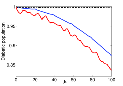
Figure 2: Diabatic population dynamics of the BMA cation: Diab-wGP (dashed black), Adiab-noGP (solid red), Diab-noGP (solid blue).

III.2 Excited state dynamics

All three systems presented in Table I are assessed here so that results of our previous studyRyabinkin, Joubert-Doriol, and Izmaylov (2014) using the Adiab-noGP approach can be contrasted with those of Diab-noGP. A Gaussian wave-packet [Eq. (16)] centred at a Franck-Condon (FC) point and placed on the excited adiabatic electronic state is taken as an initial nuclear wave-function (Table 1 and Fig. 3). The quantity characterizing excited state dynamics will be the adiabatic electronic state population $P_{\rm adi}(t)=\braket{\chi^{\text{adi}}_{2}(t)}{\chi^{\text{adi}}_{2}(t)}$, where $\chi^{\text{adi}}_{2}(x,y,t)$ is a time-dependent nuclear wave-function that corresponds to the excited adiabatic electronic state (Fig. 4).

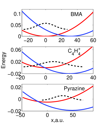
Figure 3: $y=0$ cuts of the diabatsnot (red and blue) and the initial wave-packet (black dashed) for excited state dynamics of BMA cation, $\rm C_{4}H_{4}^{+}$, and pyrazine.

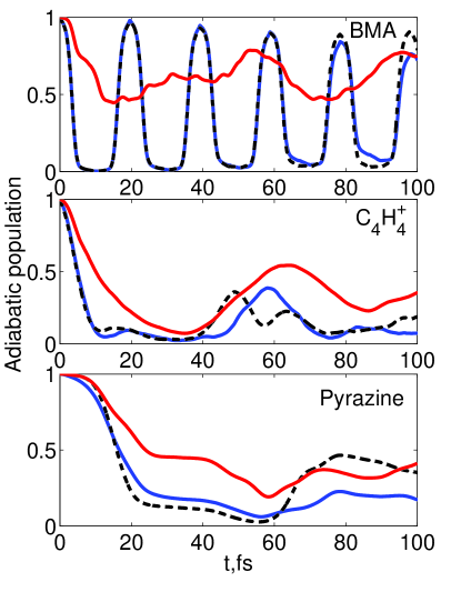
Figure 4: Excited state population dynamics of BMA cation, $\rm C_{4}H_{4}^{+}$, and pyrazine: Diab-wGP (dashed black), Adiab-noGP (solid red), Diab-noGP (solid blue).

For BMA, due to low diabatic coupling, the exact dynamics (Diab-wGP) corresponds to coherent oscillations on a donor diabatic surface. Once the wave-packet crosses the diabatic state intersection the adiabatic population switches from excited to the ground state, but the wave-packet resides almost completely on the same diabat. The period of these oscillations corresponds exactly to the tuning mode frequency $\omega_{1}=2\pi/20$ fs^-1. Switching to the Diab-noGP approach does not change dynamics within a sub 100 fs time-scale because small $c$ makes transitions between diabatic levels inefficient. In other words, the difference in the coupling structure $(n,m)_{s}\rightarrow(n^{\prime},m\pm 1)_{s^{\prime}}$ for model 1 versus $(n,m)_{s}\rightarrow(n^{\prime},m\pm 2k)_{s^{\prime}}$ for model 2 does not cause large differences in population dynamics until population transfer between diabatic states becomes appreciable. Differences between results of Adiab-noGP and Diab-wGP have been extensively discussed in Ref. Ryabinkin, Joubert-Doriol, and Izmaylov, 2014, and in BMA, they correspond to compensation of DBOC by GP induced terms in NACs. Without GP, DBOC has a significant repulsive character that prevents the wave-packet from approaching a CI region and thus hinders nonadiabatic transfer.

In the butatriene cation and pyrazine, the initial wave-packets are much closer to the CI (Fig. 3) and diabatic coupling constant $c$ is more than 5 times larger than in the BMA case. Thus, the time-scale of the adiabatic population dynamics is regulated by the nonadiabatic transition rather than oscillations on a diabatic surface. Pyrazine due to its further FC point from the CI has a small plateau region in the initial population dynamics, this plateaux corresponds to a wave-packet approach to the CI. As in the BMA case, differences between Diab-wGP and Diab-noGP appear at a longer time-scale than that of the initial nonadiabatic transition. Absence of the difference in Diab-wGP and Diab-noGP can be attributed to averaging over transitions of many diabatic vibrational states forming a wave-packet on the excited state. These vibrational states although individually may have some differences in transferring population to accepting states in two models, but for the overall transfer such differences are averaged out. The difference between Adiab-noGP and Diab-wGP is apparent even at ultra-fast initial transitions and has origin in enhancement of nonadiabatic transfer due to the GP for some parts of the nuclear wave-packet.Ryabinkin, Joubert-Doriol, and Izmaylov (2014)

IV Concluding remarks

We presented a new method of analyzing GP induced effects in dynamics. It has conceptually important aspects and practical advantages. Conceptually, it is interesting to see what are the possible ways to remove the GP and how different these ways are in terms of quantum dynamics. Previously, to remove the GP one could ignore double-valued boundary conditions of electronic and nuclear wave-functions, this led to modifying both low energy dynamics and fast excited state dynamics. The new approach shows the same effect of the GP removal for the low energy dynamics, but does not have substantial effect in the fast excited state dynamics. Practically, the new approach gives an opportunity to study GP effects in the diabatic representation where simulation methods are much more developed (e.g., Multi-configuration time-dependent Hartree approach). Thus we can easily explore $N$-dimensional scenarios without necessity for additional transformations. Going beyond linear vibronic coupling is also possible because our main modification puts absolute value on the coupling term so that in the two-electronic state problem $V_{12}$ transforms into $|V_{12}|$ without changing the adiabatic potential energy surfaces.

V Acknowledgments

A.F.I. acknowledges funding from a Sloan Research Fellowship and the Natural Sciences and Engineering Research Council of Canada (NSERC) through the Discovery Grants Program. L.J.D. is grateful to the European Union Seventh Framework Programme (FP7/2007-2013) for the financial support under grant agreement PIOF-GA-2012-332233.

References

- Balzer, Hahn, and Stock (2003) B. Balzer, S. Hahn, and G. Stock, Chem. Phys. Lett. 379, 351 (2003).
- Köppel, Domcke, and Cederbaum (1984) H. Köppel, W. Domcke, and L. S. Cederbaum, “Multimode Molecular Dynamics Beyond the Born-Oppenheimer Approximation,” (John Wiley & Sons, Inc., 1984) Chap. 2, pp. 59–246.
- Yarkony (1996) D. R. Yarkony, Rev. Mod. Phys. 68, 985 (1996).
- Hahn and Stock (2000) S. Hahn and G. Stock, J. Phys. Chem. B 104, 1146 (2000).
- Berry (1984) M. V. Berry, Proc. R. Soc. A 392, 45 (1984).
- Mead and Truhlar (1979) C. A. Mead and D. G. Truhlar, J. Chem. Phys. 70, 2284 (1979).
- Berry (1987) M. V. Berry, Proc. R. Soc. A 414, 31 (1987).
- Longuet-Higgins et al. (1958) H. C. Longuet-Higgins, U. Opik, M. H. L. Pryce, and R. A. Sack, Proc. R. Soc. A 244, 1 (1958).
- Schön and Köppel (1995) J. Schön and H. Köppel, J. Chem. Phys. 103, 9292 (1995).
- Ryabinkin and Izmaylov (2013) I. G. Ryabinkin and A. F. Izmaylov, Phys. Rev. Lett. 111, 220406 (2013).
- Joubert-Doriol, Ryabinkin, and Izmaylov (2013) L. Joubert-Doriol, I. G. Ryabinkin, and A. F. Izmaylov, J. Chem. Phys. 139, 234103 (2013).
- Hazra, Balakrishnan, and Kendrick (2015) J. Hazra, N. Balakrishnan, and B. K. Kendrick, Nature Communications 6, 1 (2015).
- Kendrick and Pack (1996) B. Kendrick and R. T. Pack, J. Chem. Phys. 104, 7475 (1996).
- Kendrick (2003) B. K. Kendrick, in Conical Intersections. Electronic Structure, Dynamics and Spectroscopy, Advanced Series in Physical Chemistry, Vol. 15, edited by W. Domcke, D. R. Yarkony, and H. Köppel (World Scientific, 2003) Chap. 12, pp. 521–553.
- Althorpe, Stecher, and Bouakline (2008) S. C. Althorpe, T. Stecher, and F. Bouakline, J. Chem. Phys. 129, 214117 (2008).
- Baer (2000) M. Baer, Chem. Phys. 259, 123 (2000).
- Note (1) Atomic units will be used throughout this paper.
- Born and Huang (1954) M. Born and K. Huang, in Dynamical Theory of Crystal Lattices (Oxford University Press, Amen House, London, 1954) p. 407.
- Handy and Lee (1996) N. C. Handy and A. M. Lee, Chem. Phys. Lett. 252, 425 (1996).
- Valeev and Sherrill (2003) E. F. Valeev and C. D. Sherrill, J. Chem. Phys. 118, 3921 (2003).
- Ryabinkin, Joubert-Doriol, and Izmaylov (2014) I. G. Ryabinkin, L. Joubert-Doriol, and A. F. Izmaylov, J. Chem. Phys. 140, 214116 (2014).
- Izmaylov et al. (2011) A. F. Izmaylov, D. Mendive-Tapia, M. J. Bearpark, M. A. Robb, J. C. Tully, and M. J. Frisch, J. Chem. Phys. 135, 234106 (2011).
- Burghardt, Giri, and Worth (2008) I. Burghardt, K. Giri, and G. A. Worth, J. Chem. Phys. 129, 174104 (2008).
- Cattarius et al. (2001) C. Cattarius, G. A. Worth, H.-D. Meyer, and L. S. Cederbaum, J. Chem. Phys. 115, 2088 (2001).
- Raab et al. (1999) A. Raab, G. A. Worth, H.-D. Meyer, and L. S. Cederbaum, J. Chem. Phys. 110, 936 (1999).
- (26) For the zero coupling line (), the diabatic and adiabatic cuts coincide up to different ordering procedures.