Macroscopic Limits of pathway-based kinetic models for E.coli chemotaxis in large gradient environments

Abstract.

It is of great biological interest to understand the molecular origins of chemotactic behavior of E. coli by developing population-level models based on the underlying signaling pathway dynamics. We derive macroscopic models for E.coli chemotaxis that match quantitatively with the agent-based model (SPECS) for all ranges of the spacial gradient, in particular when the chemical gradient is large such that the standard Keller-Segel model is no longer valid. These equations are derived both formally and rigorously as asymptotic limits for pathway-based kinetic equations. We also present numerical results that show good agreement between the macroscopic models and SPECS. Our work provides an answer to the question of how to determine the population-level diffusion coefficient and drift velocity from the molecular mechanisms of chemotaxis, for both shallow gradients and large gradients environments.

Key words: kinetic-transport equations; chemotaxis; asymptotic analysis; run and tumble; biochemical pathway;
Mathematics Subject Classification (2010): 35B25; 82C40; 92C17

1. Introduction

The movement of Escherichia coli (E. coli) presents an pattern of alternating forward-moving runs and reorienting tumbles. The run-and-tumble movements can be described by a Boltzmann type velocity jump model [12, 13]. It responds to external chemical signals by a biased random walk process. In order to develop quantitative and predictive models, we have to first understand the response of bacteria to signal changes which is a sophisticated chemotactic signal transduction pathway. Fortunately, modern experimental technologies have enabled people to quantitatively measure the details of the E.coli chemotactic sensory system [7, 11, 30, 27]. The response of E.coli to signal changes includes two steps: excitation and adaptation. Excitation is a rapid response of the cell to the external signal. It is due to the biochemical pathways regulating the flagellar motors. The slow adaptation allows the cell to subtract out the background signal. It is carried out by the relatively slow receptor methylation and demethylation processes that modulate the methylation level of receptors [9, 29, 25].

It is possible to develop predictive agent-based models thanks to the understanding of the intracellular signalling pathway. However, direct computation of agent-based models is extremely time consuming when large number of cells are evolved. Moreover, the results are usually shown to be noisy [17]. Therefore, it is of great biological interest to understand the molecular origins of chemotactic behaviour of E. coli by developing population-level model based on the underlying signalling pathway dynamics.

In order to establish quantitative connections between the agent-based models and population-level models, the usual strategy is to use mesoscopic kinetic-transport equations and derive their macroscopic limits [28]. There are two different classes of kinetic-transport models for E.coli chemotaxis in the literature. One heuristically includes tumbling frequencies depending on the path-wise gradient of chemotactic signals, while the other takes into account an intra-cellular molecular biochemical pathway and relates the tumbling frequency to this information [24]. It is possible to rescale both type of kinetic-transport models and study their diffusion and hyperbolic limits as in [5, 8, 12, 22, 26, 21].

In most previous work, in order to take into account the effects of the internal signal pathway and derive macroscopic models, moments of the internal state are used [10, 26, 27, 33, 34, 35]. The derivation is based on moment closure techniques. The moment system is usually closed by the assumption that the deviation of the internal state is not far from its expectation. This assumption is only valid when the chemical gradient is small. Macroscopic models are then derived by various asymptotic limits of the closed moment system. For example, the Keller-Segel model can be considered as a diffusion limit of the first-order moment closure, which assumes that the internal states of all bacteria are concentrated at their expectation. In [10, 33] the authors derived the macroscopic Keller-Segel equation from agent-based models by incorporating a toy linear model for the intracellular signal transduction pathways. Recently, more complicated real intracellular signalling networks that are intrinsically nonlinear are considered [26, 34]. Another model is introduced in [27], where the authors developed a pathway-based mean field theory (PBMFT). This theory is used to explain the counter-intuitive experiment which shows the mass centre of the cells does not follow the dynamics of ligand concentration in a spatial-temporal fast-varying environment [36]. PBMFT can be considered as a hyperbolic limit of the second order moment closure system [26]. However, compared with the agent-based simulations, PBMFT only recovers the right behavior for the mass centre in the spatial-temporal fast-varying environment and does not give a good match of the detailed dynamics of bacteria space distribution. One remedy proposed in [35] is to use a fourth-order moment system. Since higher-order moment systems include more information about the internal state distribution, it is reasonable to expect that they can yield better approximations. In fact, the larger the path-wise gradient is, the wider the distribution of the internal state spreads. Therefore more moments should be included. However, it is not yet fully understood what the correct number of moments one should choose to obtain an accurate approximation. This depends on how fast the environment varies, i.e. how large the space gradient is and how quickly the signal changes.

In this paper, instead of using moment closure in the internal state, we derive both formally and rigorously macroscopic models as asymptotic limits of pathway kinetic equations for E.coli chemotaxis. We also show numerically that so-derived macroscopic models match quantitatively with the agent-based model for all ranges of chemical gradients.

The pathway kinetic model we consider contains both individual bacteria movement by run-and-tumble and an intra-cellular molecular content [27]. This equation governs the evolution of the probability density function $p(x,v,m,t)$ of bacteria at time $t$, position $x\in\mathbb{R}^{d}$, velocity $v\in\mathbb{V}$, and methylation level $m>0$. In this paper, we will restrict ourselves to the discrete kinetic equation where $x\in\mathbb{R}^{1}$ and

$$\mathbb{V}=\{-v_{0},v_{0}\}\,,\qquad{\rm d}v=\frac{1}{2}\left(\delta(v-v_{0})+\delta(v+v_{0})\right)\,.$$

Here $v_{0}>0$ is the fixed speed. The general form of the kinetic equation is

$$\partial_{t}p+v\cdot\nabla_{x}p+\partial_{m}[f(m,M)p] =Q[m,M](p)\,,$$ (1.1)

where $M(x,t)$ is the methylation level at equilibrium which relates to the extra-cellular chemical signal. The function $f(m,M)$ describes the intracellular adaptation dynamics that gives the evolution of the methylation level. The tumbling term $Q[m,M](p)$ satisfies

$$Q[m,M](p)=\int_{\mathbb{V}}\left[\lambda(m,M,v,v^{\prime})p(t,x,v^{\prime},m)-\lambda(m,M,v^{\prime},v)p(t,x,v,m)\right]{\rm d}v^{\prime},$$ (1.2)

where $\lambda(m,M,v,v^{\prime})$ denotes the methylation dependent tumbling frequency from $v^{\prime}$ to $v$, in other words the response of the cell depending on its environment and internal state. The methylation level $M(x,t)$ is related to the extra-cellular attractant profile $S$ by a logarithmic dependency such that

$$M=M(S)=m_{0}+\frac{f_{0}(S)}{\alpha_{0}},\qquad\mbox{with}\quad f_{0}(S)=\ln\biggl{(}\frac{1+S/K_{I}}{1+S/K_{A}}\biggr{)}\,.$$

The constant $m_{0}$ is a reference methylation level in the absence of signal and the constants $K_{I}$ and $K_{A}$ represent the dissociation constants for inactive and active receptors respectively. They satisfy the relation that $K_{I}\ll S\ll K_{A}$. Therefore, $f_{0}(S)\approx\ln(S/K_{I})$. In this paper, we will use

$$f_{0}(S)=\ln(S/K_{I})\,,\qquad S=S_{0}e^{\int_{0}^{x}G(x^{\prime})\,{\rm d}x^{\prime}}\,.$$

Then the gradient of $M$ simplifies to

$$\partial_{x}M=G/\alpha_{0}\,.$$ (1.3)

We will consider the the case when $G$ is uniform in space, which is the exponential environment as in the experiment in [18].

As in [27], we assume that the tumbling frequency $\lambda$ is independent of $v$ and $v^{\prime}$. Moreover, the specific forms of the intracellular dynamics and the tumbling frequency are given by

$$f\big{(}m-M\big{)}=F_{0}(a)=k_{R}(1-a/a_{0})\,,\quad\lambda(m,M,v,v^{\prime})=Z(a)=z_{0}+\tau_{0}^{-1}\left(\frac{a}{a_{0}}\right)^{H},$$ (1.4)

where $a(m-M(S))$ is the receptor activity that depends on the intracellular methylation level $m$ and the extracellular chemoattractant concentration $S$ in the way that

$$a=\bigl{(}1+\exp(NE)\bigr{)}^{-1}\,,\qquad\mbox{with }E=-\alpha_{0}(m-m_{0})+f_{0}(S)=-\alpha_{0}(m-M(S)).$$ (1.5)

Here the coefficient $N$ represents the number of tightly coupled receptors. The parameter $k_{R}$ is the methylation rate, $a_{0}$ is the receptor preferred activity. The parameters $z_{0}$, $H$, $\tau_{0}$ in the tumbling frequency represent the rotational diffusion, the Hill coefficient of flagellar motors response curve, and the average run time respectively. All these parameters can be measured biologically. For more details about the derivation of these formalisms and physical meanings of these parameters, we refer the reader to [27] and the references therein.

The most widely used macroscopic (or population-level) model is the Keller-Segel equation, which was first introduced in [23]. Later, Keller and Segel used it to model chemotaxis behavior of bacteria and cells [19, 20]. It reads

$$\partial_{t}\rho=\nabla\cdot(D\nabla\rho-\kappa\rho\phi(\nabla S)).$$

The fundamental question of how to determine $D$ and $\phi(\nabla S)$ from the molecular mechanisms of chemotaxis has been studied in [27, 26, 34] using (1.1), where the molecular origins of the logarithmic sensitivity [18] of the E. coli chemotaxis is justified for slowly varying environment. However, as pointed out in [27], both Keller-Segel equation and BPMFT fail to give the right average drift velocity in the exponential environment when the chemical gradient becomes large. The valid macroscopic equation that can match quantitatively with the agent-based model for large gradient environment has been open since then and this is what we want to address in this paper. In particular, we give an answer to the question of how to determine the population level drift velocity from the molecular mechanisms of chemotaxis, for all ranges of chemical gradients. It is shown that for large chemical gradients, the leading-order macroscopic equations are hyperbolic, therefore the diffusion term is of higher order compared with the advection term. When the chemical gradient decreases, the leading-order macroscopic equation becomes the standard Keller-Segel equation with the same diffusion and advection coefficient as in [26].

The rest of the paper is organized as follows. In Section 2, we use asymptotic analysis to formally derive the leading-order macroscopic equations from (1.1). Quantitative agreement of the distribution function as well as the drift velocity of the agent based simulation and our analytical results are numerically shown in Section 3. In Section 4, we introduce various scalings to (1.1) and rigorously show the convergence of the kinetic model to the macroscopic models derived in Section 2. We then conclude in Section 5.

2. Formal Asymptotics

In this section we formally derive the leading-order macroscopic equations from the kinetic equation (1.1). Both the leading order distribution and the chemotaxis drift velocity will be derived explicitly.

Throughout this paper we will use the notation

$$\left\langle\left\langle F\right\rangle\right\rangle_{v,a}=\int_{0}^{1}\int_{\mathbb{V}}\frac{F}{N\alpha_{0}a(1-a)}{\rm d}v{\rm d}a\,,\qquad\left\langle F\right\rangle_{v}=\int_{\mathbb{V}}F{\rm d}v\,,$$

for any function $F$ which makes sense of the above integrals.

We start with reformulating equation (1.1). Since the adaptation rate $f$ is in a particularly simple form in the receptor activity $a$, we re-write equation (1.1) in $(t,x,v,a)$. To this end, let $q(t,x,v,a)=p(t,x,v,m)$. Then $q$ satisfies

$$\partial_{t}q+v\cdot\nabla_{x}q+(\partial_{a}q)(D_{t}M)\frac{\partial a}{\partial M}+\frac{\partial a}{\partial m}\partial_{a}(F_{0}(a)q)=Z(a){\mathcal{L}}q_{\epsilon}\,,$$

where $F_{0}(a)$ is defined in (1.4) and by (1.5), we have

$$\frac{\partial a}{\partial M}=-\frac{\partial a}{\partial m}=-N\alpha_{0}a(1-a)\,,\qquad{\mathcal{L}}q_{\epsilon}=\int_{\mathbb{V}}(q(t,x,v^{\prime},a)-q(t,x,v,a)){\rm d}v^{\prime}\,.$$ (2.1)

Therefore, the $q$-equation becomes

$$\partial_{t}q+v\cdot\nabla_{x}q+N\alpha_{0}a(1-a)\partial_{a}\left(\left(-D_{t}M+k_{R}\left(1-\frac{a}{a_{0}}\right)\right)q\right)=Z(a){\mathcal{L}}q_{\epsilon}\,.$$ (2.2)

The weighted average of $q$ in $a$ satisfies

$$\bar{q}(t,x,v) =\int_{0}^{1}q(t,x,v,a)\frac{\partial m}{\partial a}{\rm d}a=\int_{0}^{1}q(t,x,v,a)\frac{1}{N\alpha_{0}a(1-a)}{\rm d}a$$

$$=\int_{-\infty}^{\infty}p(t,x,v,m)\,{\rm d}m=\bar{p}(t,x,v)\,.$$

Furthermore, by the assumption (1.3), the $q$-equation simplifies to

$$\partial_{t}q+v\partial_{x}q+N\alpha_{0}a(1-a)\partial_{a}\left(\left(-\frac{v}{\alpha_{0}}G+k_{R}\left(1-\frac{a}{a_{0}}\right)\right)q\right)=Z(a){\mathcal{L}}q_{\epsilon}\,,$$ (2.3)

with $a_{0}=1/2$ as in [27].

To perform the asymptotic analysis, we introduce the small parameter $\epsilon>0$ and rescale equation (2.3) as

$$\epsilon^{\beta}\partial_{t}q_{\epsilon}+\epsilon v\partial_{x}q_{\epsilon}+N\alpha_{0}a(1-a)\partial_{a}\left(\left(-\frac{v}{\alpha_{0}}G+k_{R}\left(1-\frac{a}{a_{0}}\right)\right)q_{\epsilon}\right)=Z(a){\mathcal{L}}q_{\epsilon}\,$$ (2.4)

with $\beta\in[1,2]$. Denote the total density and the density flux as $\rho_{\epsilon}$ and $J_{\epsilon}$ such that

$$\rho_{\epsilon}(x,t)=\left\langle\left\langle q_{\epsilon}\right\rangle\right\rangle_{v,a}\,,\qquad J_{\epsilon}(x,t)=\left\langle\left\langle vq_{\epsilon}\right\rangle\right\rangle_{v,a}\,.$$

Then $\rho_{\epsilon},J_{\epsilon}$ satisfy the macroscopic equation

$$\epsilon^{\beta-1}\partial_{t}\rho_{\epsilon}+\partial_{x}J_{\epsilon}=0\,.$$ (2.5)

The main part for the asymptotic analysis is to show how to close equation (2.5). The idea is to use the leading-order distribution given by the ODE

$$N\alpha_{0}a(1-a)\partial_{a}\left(\left(-\frac{v}{\alpha_{0}}G+k_{R}\left(1-\frac{a}{a_{0}}\right)\right)q_{0}\right)=Z(a){\mathcal{L}}q_{0}\,.$$ (2.6)

The solution to the above ODE can be found explicitly and we have the following proposition:

Proposition 2.1.

Suppose the velocity space is discrete such that

$$\mathbb{V}=\{v_{0},-v_{0}\}\,,\qquad{\rm d}v=\frac{1}{2}\left(\delta(v-v_{0})+\delta(v+v_{0})\right)\,.$$

Let $q_{0}$ be a probability density function and denote

$$q_{0}^{+}=q_{0}(t,x,v_{0},a)\,,\qquad q_{0}^{-}=q_{0}(t,x,-v_{0},a)\,,$$

$$g=\frac{v_{0}}{k_{R}}\frac{G}{\alpha_{0}}\,,\qquad a_{1}=\frac{1-g}{2}\,,\qquad a_{2}=\frac{1+g}{2}\,.$$ (2.7)

(a) If $g>1$, then $a_{1}<0<1<a_{2}$. In this case the solution to (2.6) in the space of probability measures has the form

$$q_{0}^{+}(t,x,a)=\rho_{0}(t,x)c_{0}\frac{\frac{1}{2}-a_{1}}{a-a_{1}}\,\exp\left(\frac{1}{4N\alpha_{0}k_{R}}\int_{1/2}^{a}\frac{Z(\tau)}{\tau(1-\tau)}\frac{2\tau-1}{(a_{1}-\tau)(a_{2}-\tau)}\,{\rm d}\tau\right)\,\stackrel{{\scriptstyle\Delta}}{{=}}\rho_{0}Q_{0}^{+}\,,$$ (2.8)

$$q_{0}^{-}(t,x,a)=\rho_{0}(t,x)c_{0}\frac{\frac{1}{2}-a_{1}}{a_{2}-a}\,\exp\left(\frac{1}{4N\alpha_{0}k_{R}}\int_{1/2}^{a}\frac{Z(\tau)}{\tau(1-\tau)}\frac{2\tau-1}{(a_{1}-\tau)(a_{2}-\tau)}\,{\rm d}\tau\right)\,\stackrel{{\scriptstyle\Delta}}{{=}}\rho_{0}Q_{0}^{-}\,.$$ (2.9)

where $\rho_{0}$ is a probability measure and $c_{0}>0$ is determined by the normalization condition

$$\int_{\mathbb{R}}\int_{0}^{1}\frac{q^{+}_{0}+q^{-}_{0}}{2N\alpha_{0}a(1-a)}{\rm d}a\,{\rm d}x=1\,.$$ (2.10)

(b) If $0<g<1$, then $0<a_{1}<\frac{1}{2}<a_{2}<1$. In this case the solution to (2.6) in the space of probability measures has the same form as in (2.8) and (2.9) for $a\in(a_{1},a_{2})$ and

$$q_{0}^{+}=q_{0}^{-}=0\,,\qquad a\in[0,a_{1})\cup(a_{2},1]\,.$$

(c) If $g=0$, then the solution to (2.6) in the space of probability measures is

$$q_{0}^{+}=q_{0}^{-}=\frac{N\alpha_{0}}{4}\rho_{0}(t,x)\delta_{1/2}(a)\,,$$

where $\rho_{0}$ is a probability measure such that the normalization condition (2.10) holds.

Before showing the details of the proof of the above proposition, we derive the formal closures for (2.5) by using Proposition 2.1.

2.1. Formal Asymptotic Limits

We will divide the analysis according to $g={\mathcal{O}}(1)$ and $g=o(1)$. The difference between these two ranges is that in the former case, we only the leading-order distribution is used, while in the latter case we need to use the next-order correction as well.

Case I: $g={\mathcal{O}}(1)$

In this case we formally decompose $q_{\epsilon}$ according to the orders of $\epsilon$ such that

$$q_{\epsilon}=q_{0}+\epsilon q_{1}+\cdots\,.$$

By matching the terms in (2.4), we derive that the leading-order term $q_{0}$ satisfies the ODE (2.6). Let $\beta=1$ and close equation (2.5) by its leading-order approximation $q\approx q_{0}$. Then (2.5) becomes

$$\partial_{t}\int_{0}^{1}\frac{q_{0}^{+}+q_{0}^{-}}{2N\alpha_{0}a(1-a)}{\rm d}a+\partial_{x}\int_{0}^{1}\frac{v_{0}(q_{0}^{+}-q_{0}^{-})}{2N\alpha_{0}a(1-a)}{\rm d}a=0\,.$$

Therefore, from (2.8), (2.9), $\rho_{0}$ satisfies the transport equation

$$\partial_{t}\rho_{0}+\partial_{x}(\kappa_{1}\rho_{0})=0\,,\quad\text{for $g>1$}\,,$$ (2.11)

and

$$\partial_{t}\rho_{0}+\partial_{x}(\kappa_{2}\rho_{0})=0\,,\quad\text{for $0<g<1$}\,,$$ (2.12)

where if $g>1$ then the transport speed is

$$\kappa_{1} =v_{0}\left(\int_{0}^{1}\frac{Q_{0}^{+}-Q_{0}^{-}}{a(1-a)}{\rm d}a\right)\Big{/}\left(\int_{0}^{1}\frac{Q_{0}^{+}+Q_{0}^{-}}{a(1-a)}{\rm d}a\right)$$ (2.13)

$$=\frac{v_{0}}{a_{2}-a_{1}}\int_{0}^{1}\frac{1-2a}{a(1-a)}\exp\left(\frac{1}{4N\alpha_{0}k_{R}}\int_{1/2}^{a}\frac{Z(\tau)}{\tau(1-\tau)}\frac{2\tau-1}{(a_{1}-\tau)(a_{2}-\tau)}\,{\rm d}\tau\right){\rm d}a\,,$$

and if $0<g<1$, then the transport speed is

$$\kappa_{2} =v_{0}\left(\int_{a_{1}}^{a_{2}}\frac{Q_{0}^{+}-Q_{0}^{-}}{a(1-a)}{\rm d}a\right)\Big{/}\left(\int_{a_{1}}^{a_{2}}\frac{Q_{0}^{+}}{a(1-a)}{\rm d}a\right)$$ (2.14)

$$=\frac{v_{0}}{a_{2}-a_{1}}\int_{a_{1}}^{a_{2}}\frac{1-2a}{a(1-a)}\exp\left(\frac{1}{4N\alpha_{0}k_{R}}\int_{1/2}^{a}\frac{Z(\tau)}{\tau(1-\tau)}\frac{2\tau-1}{(a_{1}-\tau)(a_{2}-\tau)}\,{\rm d}\tau\right){\rm d}a\,.$$

Here $a_{1},a_{2}$ are defined in (2.7) and $Q_{0}^{\pm}$ are defined in (2.8)-(2.9).

Case II: $g=o(1)$

To be precise, we consider the case where $g={\mathcal{O}}(\epsilon^{\mu})$ with $0<\mu\leq 1$. Let

$$G_{\mu}=G/\epsilon^{\mu}={\mathcal{O}}(1)\,,\qquad g_{\mu}=\frac{v_{0}G_{\mu}}{k_{R}\alpha_{0}}={\mathcal{O}}(1)\,.$$ (2.15)

Equation (2.4) becomes

$$\epsilon^{1+\mu}\partial_{t}q_{\epsilon}+\epsilon v\partial_{x}q_{\epsilon}+N\alpha_{0}a(1-a)\partial_{a}\left(\left(-\epsilon^{\mu}v\frac{G_{\mu}}{\alpha_{0}}+k_{R}\left(1-2a\right)\right)q_{\epsilon}\right)=Z(a){\mathcal{L}}q_{\epsilon}\,,$$ (2.16)

where ${\mathcal{L}}$ is defined in (2.1). Formally decompose $q_{\epsilon}$ as

$$q_{\epsilon}=q_{0}+\epsilon^{\mu}q_{1}+o(\epsilon^{\mu})\,.$$ (2.17)

Then the leading-order equation is when $g=0$ in (2.6), which yields

$$q_{0}(t,x,v,a)=\frac{N\alpha_{0}}{4}\rho_{0}(t,x)\delta_{1/2}(a).$$ (2.18)

Meanwhile, if we denote the first few orders of $q_{\epsilon}$ up to ${\mathcal{O}}(\epsilon)$ as $\tilde{q}_{\epsilon}$, then $\tilde{q}_{\epsilon}$ satisfies the equation

$$\epsilon v\partial_{x}\tilde{q}_{\epsilon}+N\alpha_{0}a(1-a)\partial_{a}\left(\left(-v\epsilon^{\mu}G_{\mu}+k_{R}\left(1-2a\right)\right)\tilde{q}_{\epsilon}\right)=Z(a){\mathcal{L}}\tilde{q}_{\epsilon}\,.$$ (2.19)

For any fixed $\epsilon$ small enough, we have $0<a_{1}<1/2<a_{2}<1$. Thus $\tilde{q}_{\epsilon}$ is compactly supported on $[a_{1},a_{2}]=[1/2-\epsilon^{\mu}g_{\mu},1/2+\epsilon^{\mu}g_{\mu}]$. Therefore, we rewrite equation (2.19) as

$$\epsilon v\partial_{x}\tilde{q}_{\epsilon}+N\alpha_{0}a(1-a)\partial_{a}\left(\left(-v\epsilon^{\mu}G_{\mu}+k_{R}\epsilon^{\mu}\frac{1-2a}{\epsilon^{\mu}}\right)\tilde{q}_{\epsilon}\right)=Z(a){\mathcal{L}}\tilde{q}_{\epsilon}\,,$$ (2.20)

where the term $\displaystyle\frac{1-2a}{\epsilon^{\mu}}$ is uniformly bounded in $\epsilon$.

Now we separate the two cases where $0<\mu<1$ and $\mu=1$.

$\bullet$ First, if $0<\mu<1$, then by matching the terms at the leading order in (2.20), we obtain the equation for $q_{1}$ as

$$N\alpha_{0}a(1-a)\partial_{a}\left(\left(-vG_{\mu}+k_{R}\frac{1-2a}{\epsilon^{\mu}}\right)q_{0}\right)=Z(a){\mathcal{L}}q_{1}\,.$$

By (2.18) this simplifies to

$$-\frac{vG_{\mu}}{Z(a)}N\alpha_{0}a(1-a)\partial_{a}q_{0}(t,x,a)={\mathcal{L}}q_{1}\,.$$ (2.21)

Since the desired term is the flux term $J_{\epsilon}=\left\langle\left\langle vq_{1}\right\rangle\right\rangle_{v,a}$, we multiply $v$ to equation (2.21) and integrate in $v$. This gives

$$-\frac{v_{0}^{2}G_{\mu}}{Z(a)}N\alpha_{0}a(1-a)\partial_{a}q_{0}(t,x,a)=\left\langle vq_{1}\right\rangle_{v}\,.$$ (2.22)

Therefore the flux term is computed as

$$\int_{0}^{1}\left\langle vq_{1}\right\rangle_{v}\frac{1}{N\alpha_{0}a(1-a)}{\rm d}a=-\int_{0}^{1}\frac{v_{0}^{2}G_{\mu}}{Z(a)}\partial_{a}q_{0}{\rm d}a=\frac{N\alpha_{0}}{4}\rho_{0}(t,x)v_{0}^{2}G_{\mu}\left(\frac{1}{Z(a)}\right)^{\prime}\Big{|}_{a=1/2}\,.$$

Let

$$\kappa_{3}=\frac{N\alpha_{0}}{4}v_{0}^{2}G_{\mu}\left(\frac{1}{Z(a)}\right)^{\prime}\Big{|}_{a=1/2}\,.$$ (2.23)

Then the moment closure has the form

$$\partial_{t}\rho_{0}+\partial_{x}(\kappa_{3}\rho_{0})=0\,.$$ (2.24)

$\bullet$ Now we consider the case where $\mu=1$. In this case the only difference is equation (2.22) has an addition term from the advection and the new equation is

$$\frac{v_{0}^{2}}{Z(a)}\partial_{x}q_{0}-\frac{v_{0}^{2}G_{1}}{Z(a)}N\alpha_{0}a(1-a)\partial_{a}q_{0}(t,x,a)=\left\langle vq_{1}\right\rangle_{v}\,,\qquad G_{1}=G/\epsilon\,.$$ (2.25)

Integrating in $a$ gives the flux term as

$$\quad\,\int_{0}^{1}\left\langle vq_{1}\right\rangle_{v}\frac{1}{N\alpha_{0}a(1-a)}{\rm d}a$$

$$=\frac{N\alpha_{0}}{4}(v_{0}^{2}\partial_{x}\rho_{0})\int_{0}^{1}\frac{1}{Z(a)}\delta_{1/2}(a)\frac{1}{N\alpha_{0}a(1-a)}{\rm d}a-v_{0}^{2}G_{1}\frac{N\alpha_{0}}{4}\int_{0}^{1}\frac{1}{Z(a)}\partial_{a}q_{0}\,{\rm d}a$$

$$=\frac{v_{0}^{2}}{Z(1/2)}\partial_{x}\rho_{0}+\frac{N\alpha_{0}}{4}\rho_{0}(t,x)v_{0}^{2}G_{1}\left(\frac{1}{Z(a)}\right)^{\prime}\Big{|}_{a=1/2}\,.$$

Then the moment closure is the classical Keller-Segel equation:

$$\partial_{t}\rho_{0}+\partial_{x}(D_{0}\partial_{x}\rho_{0})+\partial_{x}(\kappa_{3}\rho_{0})=0\,,$$ (2.26)

where the coefficient $D_{0}$ is

$$D_{0}=\frac{v_{0}^{2}}{Z(1/2)}=\frac{v_{0}^{2}}{z_{0}+\tau_{0}^{-1}}\,,$$

and $\kappa_{3}$ is the same transport speed defined in (2.23).

Remark 2.2.

Since the distributions in $a$ for those forward and backward moving bacteria are explicitly known in (2.8), (2.9), when $g={\mathcal{O}}(\epsilon^{\mu})$, $\mu\in(0,1)$, we can not only get the leading order distribution in (2.18), but also the distribution up to ${\mathcal{O}}(\epsilon^{\mu})$. Therefore, the macroscopic equation up to ${\mathcal{O}}(\epsilon^{1-\mu})$ can be obtained as well. An additional ${\mathcal{O}}(\epsilon^{1-\mu})$ diffusion term will appear in the macroscopic equation which formally tends the diffusion in the Keller-Segel model when $\mu\to 1$.

2.2. The leading order distribution

The solution of (2.6) plays an essential role in the derivation of the macroscopic equation, we prove Proposition 2.1 and show some properties of leading order distribution in this part.

Proof of Proposition 2.1.

First note that since $q_{0}^{\pm}$ are finite measures, by (2.6) we have

$$\text{$(a_{1}-a)q_{0}^{+}$ and $(a_{2}-a)q_{0}^{-}$ are both BV functions on any $(c,d)\subsetneq(0,1)$}\,.$$

Moreover, by the normalization condition (2.10),

$$\liminf_{a\to 0}q_{0}^{\pm}(a)=\liminf_{a\to 1}q_{0}^{\pm}(a)=0\,.$$

(a) Since the velocity space $\mathbb{V}$ is discrete, we have

$$\left({\mathcal{L}}q_{0}\right)^{+}(t,x,a)=\frac{1}{2}\left(q_{0}^{-}-q_{0}^{+}\right)\,,\qquad\left({\mathcal{L}}q_{0}\right)^{-}(t,x,a)=\frac{1}{2}\left(q_{0}^{+}-q_{0}^{-}\right)\,.$$

Together with the notation introduced in (2.7), equations (2.8)-(2.9) become

$$a(1-a)\partial_{a}\left((a_{1}-a)q_{0}^{+}\right)=\frac{Z(a)}{4N\alpha_{0}k_{R}}\left(q_{0}^{-}-q_{0}^{+}\right)\,,$$ (2.27)

$$a(1-a)\partial_{a}\left((a_{2}-a)q_{0}^{-}\right)=\frac{Z(a)}{4N\alpha_{0}k_{R}}\left(q_{0}^{+}-q_{0}^{-}\right)\,.$$ (2.28)

This is a system of two ODEs which we can solve explicitly. Since the variables $t,x$ do not appear explicitly in equations (2.27)-(2.28), the solution $q_{0}$ will be in a separated form such that

$$q_{0}(t,x,v,a)=\rho_{0}(t,x)\,Q_{0}(v,a)\,,\qquad q_{0}^{\pm}(t,x,a)=\rho_{0}(t,x)\,Q_{0}^{\pm}(a)\,,$$ (2.29)

where $Q_{0}^{\pm}$ satisfy the normalization condition

$$\int_{0}^{1}\frac{Q_{0}^{+}+Q_{0}^{-}}{2N\alpha_{0}a(1-a)}{\rm d}a=1\,.$$ (2.30)

To solve (2.27)-(2.28), we add these two equations up and get

$$a(1-a)\partial_{a}\left((a_{1}-a)Q_{0}^{+}+(a_{2}-a)Q_{0}^{-}\right)=0\,.$$

Hence there exists a constant $c_{1}$ such that for $a\in(0,1)$,

$$(a_{1}-a)Q_{0}^{+}+(a_{2}-a)Q_{0}^{-}=c_{1}\,.$$ (2.31)

Now we show that $c_{1}=0$. Suppose instead $c_{1}>0$. Since $Q_{0}^{\pm}$ are both non-negative measures, we have

$$Q_{0}^{-}(a)\geq\frac{c_{1}}{a_{2}-a}\geq\frac{c_{1}}{a_{2}}\geq 0\,.$$

This contradicts the finiteness of $Q_{0}^{-}$ in (2.30). Similarly, if $c_{1}<0$, then

$$\bar{q}_{0}^{+}(a)\geq\frac{-c_{1}}{a-a_{1}}\geq\frac{-c_{1}}{1-a_{1}}\geq 0\,,$$

which also contradicts (2.30). Therefore $c_{1}=0$ and $Q_{0}^{\pm}$ satisfy

$$(a_{1}-a)Q_{0}^{+}+(a_{2}-a)Q_{0}^{-}=0\,.$$ (2.32)

This gives

$$Q_{0}^{-}=\frac{a-a_{1}}{a_{2}-a}Q_{0}^{+}\,.$$ (2.33)

Applying (2.33) in (2.27), we get for $a\in(0,1)$,

$$\partial_{a}\left((a_{1}-a)Q_{0}^{+}\right)=\frac{1}{4N\alpha_{0}k_{R}}\frac{Z(a)}{a(1-a)}\frac{2a-1}{(a_{1}-a)(a_{2}-a)}(a_{1}-a)Q_{0}^{+}\,.$$

Solving this ODE for $(a_{1}-a)\bar{q}_{0}^{+}$ gives

$$(a_{1}-a)Q_{0}^{+}=c_{0}(a_{1}-1/2)\,\exp\left(\frac{1}{4N\alpha_{0}k_{R}}\int_{1/2}^{a}\frac{Z(\tau)}{\tau(1-\tau)}\frac{2\tau-1}{(a_{1}-\tau)(a_{2}-\tau)}\,{\rm d}\tau\right)\,.$$

This combined with (2.33) gives (2.8) and (2.9). Note that we do not have concentration at $a=a_{1},a_{2}$ since $a_{1},a_{2}\notin[0,1]$.

(b) The proof of (b) is similar to (a). Note that both $(a_{1}-a)Q_{0}^{+}$ and $(a_{2}-a)Q_{0}^{-}$ are again in $BV(c,d)$ for any $(c,d)\subsetneq(0,1)$. Thus equations (2.27)-(2.28) and  (2.31) still holds on $(0,1)$. Now we show $c_{1}=0$ when $0<g<1$. In this case, $0<a_{1}<1/2<a_{2}<1$. Since $Q_{0}^{\pm}$ are non-negative measures, we have

$$(a_{1}-a)Q_{0}^{+}+(a_{2}-a)Q_{0}^{-}\geq 0\,,\qquad a\in(0,a_{1})\,,$$

$$(a_{1}-a)Q_{0}^{+}+(a_{2}-a)Q_{0}^{-}\leq 0\,,\qquad a\in(a_{2},1)\,.$$

Therefore $c_{1}=0$ and (2.32) holds. This also implies

$$Q_{0}^{+}(a)=Q_{0}^{-}(a)=0\,,\qquad a\in(0,a_{1})\cup(a_{2},1)\,.$$

Thus $Q_{0}^{\pm}$ are compactly supported on $[a_{1},a_{2}]$. Solving (2.32) gives

$$Q_{0}^{-}=\frac{a-a_{1}}{a_{2}-a}Q_{0}^{+}+c_{2}\delta_{a_{2}}(a)\,,\qquad a\in[a_{1},a_{2}]\,.$$ (2.34)

for some constant $c_{2}$. Solving (2.27) on $(a_{1},a_{2})$ then gives (2.8)-(2.9) on $(a_{1},a_{2})$ where $c_{0}>0$ may not satisfy the normalization condition since there can be concentration of $q_{0}^{+}$ at $a_{1}$ and $q_{0}^{+}$ at $a_{2}$. Now we show that there cannot be such concentrations. This is because both $(a_{1}-a)q_{0}^{+}$ and $(a_{2}-a)q_{0}^{-}$ are Lipschitz. Thus by (2.27)-(2.28), $q_{0}^{-}-q_{0}^{+}$ is in $L^{\infty}$. Hence they cannot have concentrations at $a_{2},a_{1}$ respectively. Therefore, the solution to (2.6) for $0<g<1$ is as claimed in part (b).

(c) If $g=0$, then $a_{1}=a_{2}=\frac{1}{2}$. In this case equation (2.6) becomes

$$N\alpha_{0}k_{R}a(1-a)\partial_{a}\left(\left(1-2a\right)q_{0}\right)=Z(a){\mathcal{L}}q_{0}\,,$$ (2.35)

or equations (2.27)-(2.28) become

$$a(1-a)\partial_{a}\left((1-2a)q_{0}^{+}\right)=\frac{Z(a)}{4N\alpha_{0}k_{R}}\left(q_{0}^{-}-q_{0}^{+}\right)\,,$$ (2.36)

$$a(1-a)\partial_{a}\left((1-2a)q_{0}^{-}\right)=\frac{Z(a)}{4N\alpha_{0}k_{R}}\left(q_{0}^{+}-q_{0}^{-}\right)\,.$$ (2.37)

Adding up equations (2.36)-(2.37) gives

$$N\alpha_{0}k_{R}\,a(1-a)\partial_{a}\left(\left(1-2a\right)\left(q_{0}^{+}+q_{0}^{-}\right)\right)=0\,.$$

Therefore,

$$(1-2a)\left(q_{0}^{+}+q_{0}^{-}\right)=c_{3}\,,\qquad a\in(0,1)\,,$$

for some constant $c_{3}$. Since $q_{0}^{+}+q_{0}^{-}$ is a non-negative measure, the only possible choice for $c_{3}$ is $c_{3}=0$. Hence

$$\left\langle q_{0}\right\rangle_{v}=\frac{q_{0}^{+}+q_{0}^{-}}{2}=N\alpha_{0}a(1-a)\rho_{0}(t,x)\delta_{1/2}(a)=\frac{N\alpha_{0}}{4}\rho_{0}(t,x)\delta_{1/2}(a)\,,$$

where $\rho_{0}$ is a probability measure. This implies that

$$(1-2a){\mathcal{L}}q_{0}=-(1-2a)q_{0}\,.$$

Thus multiplying (2.35) by $(1-2a)$ gives

$$N\alpha_{0}k_{R}(1-2a)a(1-a)\partial_{a}\left(\left(1-2a\right)q_{0}\right)=-Z(a)(1-2a)q_{0}\,,$$ (2.38)

By the finiteness of the measure $q_{0}$ as defined in (2.10), the boundary conditions of $(1-2a)q_{0}$ are

$$(1-2a)q_{0}=0\,,\qquad a=0,1/2,1\,.$$ (2.39)

Note that equation (2.38) shows

$$\partial_{a}((1-2a)q_{0})\begin{cases}\leq 0\,,&a<1/2\,,\\[2.0pt] \geq 0\,,&a>1/2\,.\end{cases}$$

Combined with the boundary conditions in (2.39), equation (2.38) has a unique solution (up to multiplication by $\rho_{0}(t,x)$) such that $(1-2a)q_{0}=0$. Thus the only solution to (2.35) is

$$q_{0}=\left\langle q_{0}\right\rangle_{v}=N\alpha_{0}a(1-a)\rho_{0}(t,x)\delta_{1/2}(a)=\frac{N\alpha_{0}}{4}\rho_{0}(t,x)\delta_{1/2}(a)\,.$$

∎

We can also study in more details the behaviour of the solution $q_{0}$ in Proposition 2.1 near $0,1$ when $g>1$ and near $a_{1},a_{2}$ when $0<g<1$.

Lemma 2.1.

Let $q_{0}$ be the solution to the ODE (2.6) in Proposition 2.1 and $q_{0}(t,x,v,a)=\rho_{0}(t,x)Q_{0}(v,a)$.

(a) If $g>1$, then there exists $\theta_{0},\theta_{1}>0$ such that

$$Q_{0}^{\pm}(a)={\mathcal{O}}\left(a^{\theta_{0}}\right)\,\,\text{for $a$ near 0}\,,\qquad Q_{0}^{\pm}(a)={\mathcal{O}}\left(a^{\theta_{1}}\right)\,\,\text{for $a$ near 1}\,.$$

(b) If $0<g<1$, then there exists $\theta_{2},\theta_{3}>0$ such that

$$Q_{0}^{+}(a)=\begin{cases}{\mathcal{O}}\left((a-a_{1})^{\theta_{2}-1}\right)\,,&a\to a_{1}^{+}\,,\\[2.0pt] {\mathcal{O}}\left((a_{2}-a)^{\theta_{3}}\right)\,,&a\to a_{2}^{-}\,,\end{cases}\qquad\quad Q_{0}^{-}(a)=\begin{cases}{\mathcal{O}}\left((a-a_{1})^{\theta_{2}}\right)\,,&a\to a_{1}^{+}\,,\\[2.0pt] {\mathcal{O}}\left((a_{2}-a)^{\theta_{3}-1}\right)\,,&a\to a_{2}^{-}\,.\end{cases}$$

Proof.

(a) By the definition of $q_{0}^{+}$ in (2.8), the asymptotic limit of $Q_{0}^{+}$ satisfies

$$\lim_{a\to 0}Q_{0}^{+} =c_{0}\frac{\frac{1}{2}-a_{1}}{-a_{1}}\exp\left(-\int_{0}^{1/2}\frac{A_{0}(\tau)-A_{0}(0)}{\tau}\,{\rm d}\tau\right)\lim_{a\to 0}\exp\left(-\frac{z_{0}}{4N\alpha_{0}k_{R}}\frac{1}{a_{1}a_{2}}\int_{1/2}^{a}\frac{1}{\tau}\,{\rm d}\tau\right)$$

$$=c_{0}\frac{\frac{1}{2}-a_{1}}{-a_{1}}\exp\left(-\int_{0}^{1/2}\frac{A_{0}(\tau)-A_{0}(0)}{\tau}\,{\rm d}\tau\right)2^{\theta_{0}}\lim_{a\to 0}a^{\theta_{0}}\,,$$

where

$$A_{0}(\tau)=\frac{1}{4N\alpha_{0}k_{R}}\frac{Z(\tau)(2\tau-1)}{(1-\tau)(a_{1}-\tau)(a_{2}-\tau)}\,,\qquad\theta_{0}=A_{0}(0)=-\frac{z_{0}}{4N\alpha_{0}k_{R}}\frac{1}{a_{1}a_{2}}\,.$$

The integral involving $A_{0}(\tau)$ converges at $\tau=0$ since $A_{0}\in C^{1}([0,1/2])$. Moreover, $\theta_{0}>0$ since $a_{1}<0<a_{2}$ and $z_{0}>0$. This shows $Q_{0}^{+}$, as well as $Q_{0}^{-}$, decays to zero algebraically at $a=0$. Note that since $z_{0}$ is generally small, the rate of decay can be sublinear.

Similarly, near $a=1$ the asymptotic limit of $Q_{0}^{+}$ is

$$\quad\,\lim_{a\to 1}Q_{0}^{+}$$

$$=c_{0}\frac{\frac{1}{2}-a_{1}}{1-a_{1}}\exp\left(\int^{1}_{1/2}\frac{A_{1}(\tau)-A_{1}(1)}{1-\tau}\,{\rm d}\tau\right)\lim_{a\to 1}\exp\left(-\frac{2^{H}}{4N\alpha_{0}k_{R}}\frac{1}{(1-a_{1})(a_{2}-1)}\int_{1/2}^{a}\frac{1}{1-\tau}\,{\rm d}\tau\right)$$

$$=c_{0}\frac{\frac{1}{2}-a_{1}}{1-a_{1}}\exp\left(\int^{1}_{1/2}\frac{A_{1}(\tau)-A_{1}(1)}{1-\tau}\,{\rm d}\tau\right)2^{\theta_{1}}\lim_{a\to 1}(1-a)^{\theta_{1}}\,,$$

where

$$A_{1}(\tau)=\frac{1}{4N\alpha_{0}k_{R}}\frac{Z(\tau)(2\tau-1)}{\tau(a_{1}-\tau)(a_{2}-\tau)}\,,\qquad\theta_{1}=A_{1}(1)=\frac{2^{H}}{4N\alpha_{0}k_{R}}\frac{1}{(1-a_{1})(a_{2}-1)}\,.$$

Again since $A_{1}\in C^{1}([1/2,1])$, the integral involving $A_{1}$ converges at $\tau=1$. We also have an algebraic decay to zero for $Q_{0}^{\pm}$ as $a\to 1$. In this case since $H$ is generally large (for example $H=10$ in our numerical example), the decay near $a=1$ is nearly exponential.

(b) Similar as in part (a), we have near $a_{1}$ the asymptotic limit of $Q_{0}^{+}$ is

$$\quad\,\lim_{a\to a_{1}^{+}}Q_{0}^{+}$$

$$=c_{0}\exp\left(-\int^{1/2}_{a_{1}}\frac{A_{2}(\tau)-A_{2}(a_{1})}{a_{1}-\tau}\,{\rm d}\tau\right)\lim_{a\to a_{1}^{+}}\frac{\frac{1}{2}-a_{1}}{a-a_{1}}\exp\left(-\frac{Z(a_{1})}{4N\alpha_{0}k_{R}}\frac{1}{a_{1}(1-a_{1})}\int_{1/2}^{a}\frac{1}{a_{1}-\tau}\,{\rm d}\tau\right)$$

$$=c_{0}\left(\frac{1}{2}-a_{1}\right)\exp\left(-\int^{1/2}_{a_{1}}\frac{A_{2}(\tau)-A_{2}(a_{1})}{a_{1}-\tau}\,{\rm d}\tau\right)\left(\frac{2k_{R}}{v_{0}G}\right)^{\theta_{2}}\lim_{a\to a_{1}^{+}}(a-a_{1})^{\theta_{2}-1}\,,$$

where

$$A_{2}(\tau)=\frac{1}{4N\alpha_{0}k_{R}}\frac{Z(\tau)(2\tau-1)}{\tau(1-\tau)(a_{2}-\tau)}\,,\qquad\theta_{2}=A_{2}(a_{1})=\frac{Z(a_{1})}{4N\alpha_{0}k_{R}}\frac{1}{a_{1}(1-a_{1})}\,.$$

The integral involving $A_{2}$ converges at $a=a_{1}$ since $A_{2}\in C^{1}([a_{1},a_{2}])$. Then by (2.9),

$$\lim_{a\to a_{1}^{+}}Q_{0}^{-}=c_{0}\frac{\frac{1}{2}-a_{1}}{a_{2}-a_{1}}\exp\left(-\int^{1/2}_{a_{1}}\frac{A_{2}(\tau)-A_{2}(a_{1})}{a_{1}-\tau}\,{\rm d}\tau\right)\left(\frac{2k_{R}}{v_{0}G}\right)^{\theta_{2}}\lim_{a\to a_{1}^{+}}(a-a_{1})^{\theta_{2}}\,.$$

Similarly, near $a_{2}$, we have

$$\lim_{a\to a_{2}^{-}}Q_{0}^{+} =c_{0}\exp\left(\int_{1/2}^{a_{2}}\frac{A_{3}(\tau)-A_{3}(a_{2})}{a_{2}-\tau}\,{\rm d}\tau\right)\frac{\frac{1}{2}-a_{1}}{a_{2}-a_{1}}\lim_{a\to a_{2}^{-}}\exp\left(-\frac{Z(a_{2})}{4N\alpha_{0}k_{R}}\frac{1}{a_{2}(1-a_{2})}\int_{1/2}^{a}\frac{1}{a_{2}-\tau}\,{\rm d}\tau\right)$$

$$=c_{0}\exp\left(\int_{1/2}^{a_{2}}\frac{A_{3}(\tau)-A_{3}(a_{2})}{a_{2}-\tau}\,{\rm d}\tau\right)\frac{\frac{1}{2}-a_{1}}{a_{2}-a_{1}}\left(\frac{2k_{R}}{v_{0}G}\right)^{\theta_{3}}\lim_{a\to a_{2}^{-}}(a_{2}-a)^{\theta_{3}}\,,$$

where

$$A_{3}(\tau)=\frac{1}{4N\alpha_{0}k_{R}}\frac{Z(\tau)(2\tau-1)}{\tau(1-\tau)(a_{1}-\tau)}\,,\qquad\theta_{3}=A_{3}(a_{2})=\frac{Z(a_{2})}{4N\alpha_{0}k_{R}}\frac{1}{a_{2}(1-a_{2})}\,.$$

Again the integral involving $A_{3}$ converges at $a=a_{2}$ since $A_{3}\in C^{1}([a_{1},a_{2}])$. Using (2.9) again we have

$$\lim_{a\to a_{2}^{-}}Q_{0}^{-}=c_{0}\exp\left(\int_{1/2}^{a_{2}}\frac{A_{3}(\tau)-A_{3}(a_{2})}{a_{2}-\tau}\,{\rm d}\tau\right)\left(\frac{1}{2}-a_{1}\right)\left(\frac{2k_{R}}{v_{0}G}\right)^{\theta_{3}}\lim_{a\to a_{2}^{-}}(a_{2}-a)^{\theta_{3}-1}\,.$$

∎

Remark 2.3.

Here the value of $\theta_{k}$ ($0\leq k\leq 3$) determines the behaviour of $q_{0}^{\pm}$ ($q_{0}^{-}$) near $a=0,1$ or $a=a_{1},a_{2}$. Since $\theta_{k}>0$ for all $0\leq k\leq 3$, the integrability in the normalization condition (2.30) is guaranteed. We note the following differences between $g>1$ and $0<g<1$:

• If $g>1$, then $q_{0}^{\pm}\to 0$ algebraically as $a\to 0$ or $a\to 1$. The decay rate is given by $\theta_{0}$ near $a=0$ and $\theta_{1}$ near $a=1$.

• If $0<g<1$, then $0<a_{1}<1/2<a_{2}<1$. In this case

  $$Z(a_{1}) =z_{0}+\tau_{0}^{-1}(a_{1}/a_{0})^{H}=z_{0}+\tau_{0}^{-1}(2a_{1})^{H}\,,$$

  $$Z(a_{2}) =z_{0}+\tau_{0}^{-1}(a_{2}/a_{0})^{H}=z_{0}+\tau_{0}^{-1}(2a_{2})^{H}\,.$$

  Thus depending on the values of $z_{0},\tau_{0}$ and $H$, the parameter $\theta_{2}$ can be less than 1 for some $a_{1}\in(0,a_{0})$, in which case we have $\lim_{a\to a_{1}^{+}}q_{0}^{+}=\infty$ with the growth rate $1-\theta_{2}$. However, when $a_{2}$ is close to $0$, by its definition $\theta_{2}$ can increase to be larger than $1$. Then $\lim_{a\to a_{1}^{+}}q_{0}^{+}=0$. On the other hand, since $H$ is large, the parameter $\theta_{3}$ is more likely to be larger than $1$.

  Using the particular physical parameters for wild type E.coli in section 3, we do have $\theta_{2},\theta_{3}>~{}1$ for all $a_{1}\in(0,1/2)$ and $a_{2}\in(1/2,1)$. Hence in Section 3 we have algebraic decay of $Q_{0}^{\pm}$ near both $a_{1}$ and $a_{2}$.

3. Comparison with Numerics

In this section we specify various types of scalings and compare the numerical results using the agent-based model SPECS and the closures derived in Section 2. Recall that the intracellular dynamics and tumbling frequency are given by

$$f\big{(}m-M(S)\big{)}=F_{0}(a)=k_{R}(1-a/a_{0})\,,\qquad\Lambda\big{(}m-M(S)\big{)}=Z(a)=z_{0}+\tau_{0}^{-1}\left(\frac{a}{a_{0}}\right)^{H},$$

where $a(m-M(S))$ is the receptor activity defined in (1.5). The parameters are chosen as in [27] such that

$$v_{0}=\frac{16.5}{\sqrt{2}}\mu m/s,\quad k_{R}=0.01s^{-1}\sim 0.0005s^{-1},\quad a_{0}=0.5,$$

$$\alpha_{0}=1.7,\quad z_{0}=0.14s^{-1},\quad\tau_{0}=0.8s,\quad H=10.$$

The external signal is given by $S=S_{0}\exp(Gx)$, where $G$ takes the values $0\sim 2*10^{-3}\mu m^{-1}$. Since $f_{0}(S)$ can be approximated by $\ln(S/K_{I})$ when $18.2\mu M=K_{I}\ll S\ll K_{A}=3mM$, we consider $S_{0}=4K_{I}$ and choose the space domain such that $5K_{I}<S(x)\leq K_{A}/5$. Therefore, the computational domain depends on $G$.

Let $T,L$ be the characteristic time and space scale for the movement on the population level. Let $T_{M},L_{M}$ be the characteristic time and length for the outside signal. We nondimensionalize equation (2.2) by letting

$$t=T\tilde{t}\,,\qquad x=L\tilde{x}\,,\qquad v_{0}=V_{0}\tilde{v}\,,\qquad k_{R}=\frac{1}{T_{a}}\tilde{k}_{R}\,,\qquad Z(a)=\frac{1}{T_{t}}\tilde{Z}(a)\,,$$

where $T_{a}$ and $T_{t}$ are the characteristic adaptation time and tumbling time respectively. Let

$$\tilde{q}(\tilde{t},\tilde{x},v,a)=q(t,x,v,a)\,,\qquad\tilde{M}(\tilde{t},\tilde{x})=M(t,x)\,.$$

Then the equation for $\tilde{q}$ becomes

$$\frac{L}{TV_{0}}\partial_{\tilde{t}}\tilde{q}+\tilde{v}\partial_{\tilde{x}}\tilde{q}+N\alpha_{0}a(1-a)\partial_{a}\left(\left(-\frac{L}{V_{0}T_{M}}\partial_{\tilde{t}}\tilde{M}-\frac{L}{L_{M}}\tilde{v}\partial_{\tilde{x}}\tilde{M}+\frac{L}{V_{0}T_{a}}\tilde{k}_{R}\left(1-\frac{a}{a_{0}}\right)\right)\tilde{q}\right)$$

$$=\frac{L}{V_{0}T_{t}}\tilde{Z}(a)\int_{\mathbb{V}}(\tilde{q}(\tilde{t},\tilde{x},v^{\prime},a)-\tilde{q}(\tilde{t},\tilde{x},v,a)){\rm d}v^{\prime}\,.$$ (3.1)

In the exponential environment, let

$$T_{M}=\infty\,,\qquad V_{0}=10\mu m/s\,.$$

The scalings for Case I and II in the previous section correspond to

• In case I where $g={\mathcal{O}}(1)$, let

  $$\epsilon=\frac{V_{0}T_{a}}{L}=\frac{V_{0}T_{t}}{L}=\frac{L_{M}}{L}\,.$$

  Then

  $$g={\mathcal{O}}\left(\frac{V_{0}T_{a}}{L_{M}}\right)={\mathcal{O}}(1)\,.$$

  Hence equation(3) becomes equation (2.4).

• In case II, let

  $$\epsilon=\frac{V_{0}T_{a}}{L}=\frac{V_{0}T_{t}}{L}\,,\qquad\epsilon^{\mu}=\frac{L}{TV_{0}}\,,\qquad\epsilon^{1-\mu}=\frac{L_{M}}{L}\,,$$

  Then

  $$g={\mathcal{O}}\left(\frac{V_{0}T_{a}}{L_{M}}\right)={\mathcal{O}}\left(\frac{V_{0}T_{a}}{L}\right){\mathcal{O}}\left(\frac{L}{L_{M}}\right)=\epsilon^{\mu}\,.$$

  Thus equation (3) becomes equation (2.16).

In [27], the authors developed a macroscopic pathway-based mean field theory (PBMFT) which successfully explained a counter-intuitive experimental observation: there exists a phase shift between the dynamics of ligand concentration and centre of mass of the cells in a spatial-temporal fast-varying environment,. However, PBMFT fails to give the right macroscopic drift velocity in the exponential environment with large gradients.

In the rest of this section we compare our results with SPECS and PBMFT. Exponential environment is considered and we use periodic boundary conditions in space, i.e. in SPECS, each bacterial that runs out of the right (left) boundary of computational domain will enter again from the left (right) with the same activity $a$.

• Comparison of the distribution in $a$. We compute the distribution of the bacteria in $a$ in two ways: one is to run SPECS and count the number of bacteria with $a$ in a small interval; the other is to compute $\frac{q_{0}^{+}}{N\alpha_{0}a(1-a)}$, $\frac{q_{0}^{-}}{N\alpha_{0}a(1-a)}$ analytically according to (2.8), (2.9). We can see that the analytical distribution yields almost the same distribution as SPECS. Moreover, the average drift velocity of our macroscopic model matches well with SPECS, while the part that the PBMFT is no longer valid is in Case I and Case II with $0<g<1$ where the hyperbolic scaling applies.

  The formal asymptotic analysis in section 2 shows that the classification of the various cases depends on the size of $g=\frac{vG}{\alpha_{0}k_{R}}$. Then for a given $k_{R}$, we can divide the value of $G$ into several intervals, where each interval corresponds to one case. Fix $k_{R}=0.005s^{-1}$. Then

  $$g=1\Leftrightarrow G=7.4*10^{-4}\mu m^{-1}\,,\qquad g=0.1\Leftrightarrow G=7.4*10^{-5}\mu m^{-1}\,,$$

  $$g=0.01\Leftrightarrow G=7.4*10^{-6}\mu m^{-1}\,,\qquad g<0.01\Leftrightarrow G<7.4*10^{-6}\mu m^{-1}\,.$$

  Thus we can divide the range of $G$ as

  • $G>7.4*10^{-4}\mu m^{-1}$: Case I with $g>1$. In this case the leading-order distribution $q_{0}$ spreads over $a\in(0,1)$. The macroscopic density $\rho_{0}$ satisfies a hyperbolic equation.

  • $G\in(7.4*10^{-5}\mu m^{-1},7.4*10^{-4}\mu m^{-1})$: Case I with $0<g<1$. In this case the leading-order distribution $q_{0}$ is compactly supported on $[a_{1},a_{2}]$. The macroscopic density $\rho_{0}$ satisfies a hyperbolic equation.

  • $G\in(7.4*10^{-6}\mu m^{-1},7.4*10^{-5}\mu m^{-1})$: Case II with $0<\mu<1$. In this case the leading-order distribution $q_{0}$ is concentrated at $a=1/2$. The macroscopic density $\rho_{0}$ satisfies a hyperbolic equation.

  • $G<7.4*10^{-6}\mu m^{-1}$: Case II with $\mu=1$. In this case the leading-order distribution $q_{0}$ is concentrated at $a=1/2$. The macroscopic density $\rho_{0}$ satisfies the Keller-Segel equation.

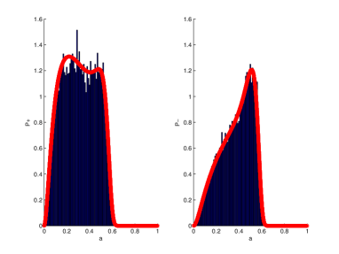
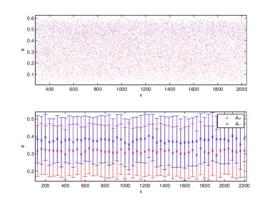
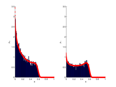
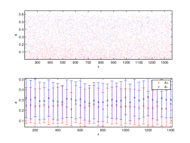
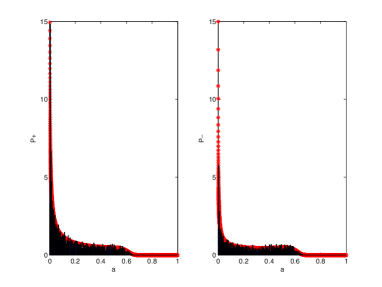
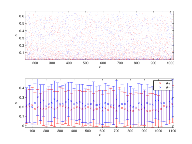
Figure 1. The distribution of $\frac{q_{0}^{+}}{N\alpha_{0}a(1-a)}$ (left) and $\frac{q_{0}^{-}}{N\alpha_{0}a(1-a)}$ (right) in $a$ for different $G$. a) b): $G=1*10^{-3}$; c) d) : $G=1.5*10^{-3}$; e) f): $G=2*10^{-3}$ when $k_{R}=0.005\mu m^{-1}$. These values all correspond to Case I with $g>1$. a) c) e): The comparison of the distribution in $a$ for forward moving bacteria (left) and backward moving bacteria (right). The bars are the results from SPECS and the solid lines are from the analytical formula in (2.8)-(2.9). b) d) f): The distribution of $a$ obtained by SPECS: red is for the forward moving bacteria and blue for the backward. The top subplots display the space distribution of bacteria with $a$ being the vertical axis. The bottom subplots give the mean and variance of $a$ at different positions.

  Figure 1 and 2 shows the analytical distributions given by the asymptotic analysis in Section 2 yield almost the same distributions as SPECS. As $G$ increases, more and more bacteria become concentrated near $a=0$. This indicates that the tumbling frequency of the bacteria becomes low. The density distribution is concentrated near $a=0.5$ for $G$ small and it spreads out when $G$ increase. The moment closure techniques in all previous paper [10, 33, 26, 27] have used the assumption that the methylation level is not far away from its average, so that it is possible to use the Taylor expansion near the average to approximate the distribution in the internal state. This assumption fails in the large-gradient environment.

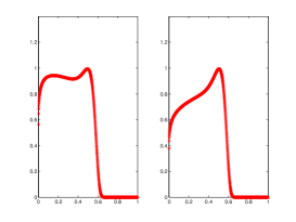
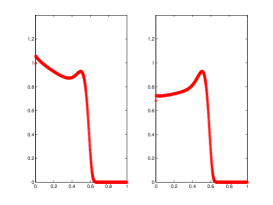
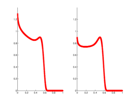
Figure 3. Each figure gives the distribution in $a$ for forward moving bacteria (left) and backward moving bacteria (right) when $k_{R}=0.0005s^{-1}$. Left: $G=3.7*10^{-4}$, $\theta_{0}=1.1072$; Middle: $G=3.9*10^{-4}$, $\theta_{0}=0.9925$; Right: $G=4.0*10^{-4}$, $\theta_{0}=0.9419$. All these values correspond to Case I with $g>1$.

• The distribution of $\frac{q_{0}^{+}}{N\alpha_{0}a(1-a)}$ and $\frac{q_{0}^{-}}{N\alpha_{0}a(1-a)}$ near $a=0$. According to the analytical formulas in (2.8)-(2.9), if $\theta_{0}=-\frac{z_{0}}{4N\alpha_{0}k_{R}}\frac{1}{a_{1}a_{2}}>1$, then $\frac{q_{0}^{\pm}}{N\alpha a(1-a)}\to 0$ as $a\to 0$. If $0<\theta_{0}<1$, then $\frac{q_{0}^{\pm}}{N\alpha a(1-a)}\to+\infty$ as $a\to 0$. This can be considered as a phase transition of the density distribution at $a=0$, which can be seen from Figure 3. The different distributions of $q_{0}^{+}$ near $a=0$ for different cases are harder to distinguish from the SPECS simulation.

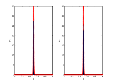
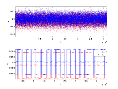
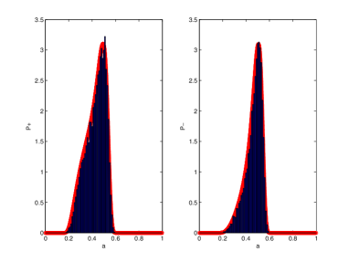
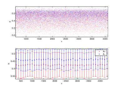
Figure 2. The distribution of $\frac{q_{0}^{+}}{N\alpha_{0}a(1-a)}$(left) and $\frac{q_{0}^{-}}{N\alpha_{0}a(1-a)}$ (right) in $a$ for different $G$’s when $k_{R}=0.005\mu m^{-1}$. a) b): $G=5*10^{-5}$ (Case II with $0<\mu<1$); c) d) : $G=5*10^{-4}$ (Case I with $0<g<1$). a) c): The comparison of the distribution in $a$ for forward moving bacteria (left) and backward moving bacteria (right). The bars are the results from SPECS and the solid lines are from the analytical formula in (2.8)-(2.9). b) d): The distribution of $a$ obtained by SPECS: red is for the forward moving bacteria and blue for the backward. The top subplots display the space distribution of bacteria with $a$ being the vertical axis. The bottom subplots give the mean and variance of $a$ at different positions.

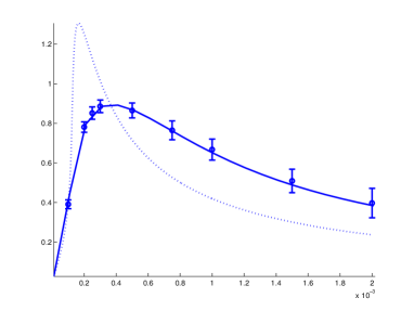
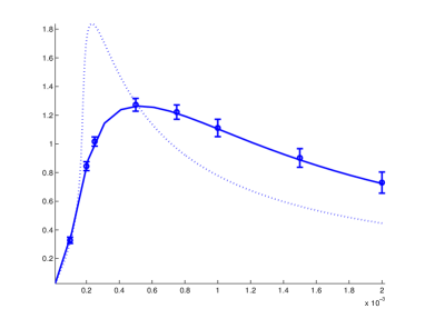
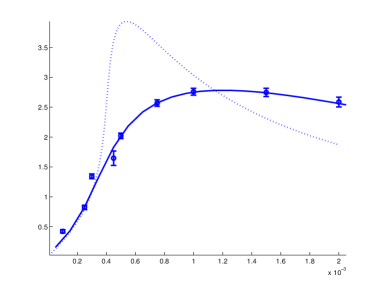
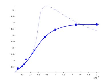
Figure 4. Average chemotaxis velocity in exponential concentration gradient for different $k_{R}$. a): $k_{R}=0.0005s^{-1}$; b): $k_{R}=0.001s^{-1}$; c): $k_{R}=0.005s^{-1}$; d): $k_{R}=0.01s^{-1}$. Here the solid lines are calculated from the analytical formula (2.13), the error bars with circles are the results by SPECS simulations and the dotted lines are the prediction by PBMFT.

• Comparison of the average drift velocity for different $k_{R}$’s and different $G$’s. From Figure 1 and Figure 2, we can observe that the distribution in $a$ is almost uniform in space, while the fluctuation in space increases with $G$. We compute the average drift velocity analytically both by (2.13) and by SPECS. In the SPECS simulation, the population-level drift velocity is obtained by counting the difference between the number of forward and backward moving bacteria and multiply it by $v_{0}$. In Figure 4 we compare the average drift velocity obtained by these two methods as well as by PBMFT in [27]. The authors pointed out in [27] that the average drift velocity will saturate when $G$ increases. This is due to the particular stopping criteria that is used to determined when the system has arrived at a steady state. If instead we run the SPECS code for a longer time until the mean and variance of the average drift velocities do not change much, then the average drift velocities do not saturate but decrease when $G$ is large enough. As has already been observed in [27], PBMFT can not give the right prediction of the population level chemotaxis velocity when $G$ becomes large while our analytical results match well with SPECS.

4. Rigorous Derivation

In this section, we rigorously derive the macroscopic models in all the cases in Section 2.

4.1. Well-posedness

The well-posedness of the kinetic equation (1.1) will be established in the space of probability measures. To this end, we introduce a few notations from mass transportation. The space we will consider is ${\mathcal{P}}_{1}({\mathbb{X}})$, the probability space on the metric space ${\mathbb{X}}$ with finite first moments. In this paper, the metric space ${\mathbb{X}}$ is ${\mathbb{X}}=\mathbb{R}\times\mathbb{V}\times(0,1)$ where $\mathbb{R}$ and $(0,1)$ are equipped with the usual Euclidean metric and $\mathbb{V}$ is a bounded space with a unit measure ${\rm d}v$. We use the 1-Wasserstein distance on ${\mathcal{P}}_{1}({\mathbb{X}})$ defined by

$$W_{1}(\mu,\nu)=\sup\left\{\int_{{\mathbb{X}}}\phi(x)\left(\,{\rm d}\mu-\,{\rm d}\nu\right)\Big{|}\left\lVert\phi\,\right\rVert_{Lip}\leq 1\right\}\,,\qquad\mu,\nu\in{\mathcal{P}}_{1}\,.$$

Let $E$ be a vector field and $X$ be transported by $E$ as

$$\frac{{\rm d}X}{\,{\rm d}t}=E(t,X)\,,\qquad X(0,x_{0})=x_{0}\,.$$

Denote the associated flow map as ${\mathcal{T}}$ such that ${\mathcal{T}}x_{0}=X$. The push-forward operator ${\mathcal{T}}^{t}_{E}\#f_{0}$ is defined as

$$\int_{{\mathbb{X}}}\xi(x)\left({\mathcal{T}}^{t}_{E}\#f_{0}\right)(t,x)\,{\rm d}x=\int_{{\mathbb{X}}}\xi({\mathcal{T}}x_{0})f_{0}(x_{0})\,{\rm d}x_{0}\,,$$

for any $\xi\in C_{b}({\mathbb{X}})$ where $C_{b}({\mathbb{X}})$ is the space of continuous and bounded functions on ${\mathbb{X}}$. For regular enough $E$ and $f_{0}$, the push-forward operator gives the solution to the transport equation

$$\partial_{t}f+\nabla_{x}\cdot\left(E(t,x)f\right)=0\,,\qquad f(0,x)=f_{0}(x)\,.$$

Define

$$\hat{q}=\frac{q}{N\alpha_{0}a(1-a)}\,.$$

Then the equation for $\hat{q}$ becomes

$$\partial_{t}\hat{q}+v\partial_{x}\hat{q}+\partial_{a}\left(\left(-vG+k_{R}\left(1-\frac{a}{a_{0}}\right)\right)N\alpha_{0}a(1-a)\hat{q}\right)=Z(a)\int_{\mathbb{V}}(\hat{q}(t,x,v^{\prime},a)-\hat{q}(t,x,v,a)){\rm d}v^{\prime}\,.$$ (4.1)

The characteristic equation associated with equation (4.1) is

$$\frac{\,{\rm d}x}{\,{\rm d}t} =v\,,$$

$$\frac{{\rm d}a}{\,{\rm d}t} =\left(-vG+k_{R}\left(1-\frac{a}{a_{0}}\right)\right)N\alpha_{0}a(1-a)\,,$$

$$\frac{{\rm d}v}{\,{\rm d}t} =0\,.$$

Thus the vector field $E$ is

$$E(t,x,a,v)=\left(v,\,\,\left(-vG+k_{R}\left(1-\frac{a}{a_{0}}\right)\right)N\alpha_{0}a(1-a),\,\,0\right)\,,$$ (4.2)

which is globally Lipschitz for each given $G$.

Definition 4.1.

The measure-value solution to equation (2.3) is defined as the measure

$$q=N\alpha_{0}a(1-a)\hat{q}\,,$$

where $\hat{q}\in C([0,T);{\mathcal{P}}_{1}\left(\mathbb{R}\times\mathbb{V}\times(0,1))\right)$ satisfies

$$\hat{q}(t,x,a,v)={\mathcal{T}}^{t}_{E}\#\hat{q}^{in}+\int_{0}^{t}{\mathcal{T}}^{t-s}_{E}\#{\mathcal{L}}\hat{q}(s,x,a,v)\,{\rm d}s\,.$$ (4.3)

Here $E$ is given in (4.2) and

$$\hat{q}^{in}=\frac{q^{in}}{N\alpha_{0}a(1-a)}\in{\mathcal{P}}_{1}\,,\qquad{\mathcal{L}}\hat{q}=\left\langle\hat{q}\right\rangle_{v}-\hat{q}\,.$$

We recall one lemma from [3]:

Lemma 4.1 (Lemma 3.18 in [3]).

Let ${\mathcal{T}}:{\mathbb{X}}\to{\mathbb{X}}$ be a globally Lipschitz map and $f,g\in{\mathcal{P}}_{1}({\mathbb{X}})$. Then

$$W_{1}({\mathcal{T}}\#f,{\mathcal{T}}\#g)\leq Lip({\mathcal{T}})W_{1}(f,g)\,,$$

where $Lip({\mathcal{T}})$ is the Lipschitz constant of ${\mathcal{T}}$.

Applying Lemma 4.1 to ${\mathcal{T}}={\mathcal{T}}^{t}_{E}$ gives

Lemma 4.2.

Let $\hat{q}^{in}_{1},\hat{q}^{in}_{2}\in{\mathcal{P}}_{1}({\mathbb{X}})$ and ${\mathcal{T}}^{t}_{E}$ be the flow map with vector field $E$ given in (4.2). Then

$$W_{1}\left({\mathcal{T}}^{t}_{E}\#\hat{q}^{in}_{1},{\mathcal{T}}^{t}_{E}\#\hat{q}^{in}_{2}\right)\leq e^{tLip(E)}W_{1}\left(\hat{q}^{in}_{1},\hat{q}^{in}_{1}\right)\,.$$

Proof.

By Lemma 4.1, we only need to estimate the Lipschitz bound of ${\mathcal{T}}^{t}_{E}$. Let $X=(x,a,v)$. Then

$$\frac{{\rm d}X}{\,{\rm d}t}=E(X)\,,\qquad X\big{|}_{t=0}=x\,.$$

Therefore, for any given initial states $x,y$, we have

$$\frac{\rm d}{\,{\rm d}t}\lvert T^{t}_{E}(x)-T^{t}_{E}(y)\rvert=\frac{\rm d}{\,{\rm d}t}\lvert X-Y\rvert\leq\lvert E(X)-E(Y)\rvert\leq Lip(E)\lvert X-Y\rvert\,.$$

By Gronwall’s inequality, we have

$$\lvert T^{t}_{E}(x)-T^{t}_{E}(y)\rvert\leq e^{tLip(E)}\lvert x-y\rvert\,.$$

∎

The main well-posedness result states

Theorem 4.1.

Suppose the intracellular dynamics and tumbling frequency are defined by (1.4) with $G$ given. Suppose the initial data $q^{in}$ satisfies

$$\frac{q^{in}}{N\alpha_{0}a(1-a)}\in{\mathcal{P}}_{1}\left(\mathbb{R}\times\mathbb{V}\times(0,1)\right)\,.$$

Then

• for any $T>0$, equation (4.1) has a unique solution $\hat{q}\in C([0,T);{\mathcal{P}}_{1}(\mathbb{R}\times\mathbb{V}\times\mathbb{R}^{+}))$ in the sense of (4.3).

• Let $S(t)$ be the solution operator to equation (4.1). Then the equation is stable in the sense that

  $$W_{1}(S(t)\hat{q}^{in}_{1},S(t)\hat{q}^{in}_{2})\leq e^{(Lip(E)+2)t}W_{1}(\hat{q}^{in}_{1},\hat{q}^{in}_{2})\,,$$ (4.4)

  where $Lip(E)$ is the global Lipschitz constant of $E$.

Proof.

For the ease of notation, in this proof we always denote

$${\mathbb{X}}=\mathbb{R}\times\mathbb{V}\times(0,1)\,.$$

The well-posedness of (4.3) will be shown by a fixed-point argument. We comment that if the initial data is smooth enough, such as $\hat{q}^{in}\in L^{\infty}({\mathbb{X}})$ with a bounded second moment, then the well-posedness has been established in the literature [24]. In this case one has the maximum principle such that if $\hat{q}^{in}\geq 0$, then $\hat{q}\geq 0$ for all $t\in[0,T)$.

For the measure-valued case, denote the operator $\Gamma$ as

$$\Gamma\hat{q}={\mathcal{T}}^{t}_{E}\#\hat{q}^{in}+\int_{0}^{t}{\mathcal{T}}^{t-s}_{E}\#{\mathcal{L}}\hat{q}(s,x,a,v)\,{\rm d}s\,.$$

Define the space $C([0,T);{\mathcal{P}}_{1}^{+}({\mathbb{X}}))$ as

$$\quad\,C([0,T);{\mathcal{P}}_{1}^{+}({\mathbb{X}}))$$

$$=\left\{\mu\in C([0,T);{\mathcal{P}}_{1}({\mathbb{X}}))\Big{|}\Gamma^{k}\mu\,\,\text{is a nonnegative measure for any $t\in[0,T)$ and any $k\geq 1$}\right\}\,.$$

Note that $C([0,T);{\mathcal{P}}_{1}^{+}({\mathbb{X}}))$ is non-empty since it contains all the regular solutions with $\hat{q}^{in}\geq 0$. The metric on $C([0,X);{\mathcal{P}}_{1}^{+}({\mathbb{X}}))$ is

$$d\left(\hat{q}_{1},\hat{q}_{2}\right)=\sup_{[0,T)}W_{1}\left(\hat{q}_{1}(t,\cdot),\hat{q}_{2}(t,\cdot)\right)\,.$$

We will show that $\Gamma$ is a contraction mapping on a convex subset of $C([0,X);{\mathcal{P}}_{1}^{+}({\mathbb{X}}))$ for $T$ small enough. First, given $\hat{q}\in C([0,T);{\mathcal{P}}_{1}^{+}({\mathbb{X}}))$, we verify that $\Gamma\hat{q}\in C([0,T);{\mathcal{P}}_{1}^{+}({\mathbb{X}}))$. Indeed, for each fixed $t$, $\Gamma\hat{q}$ is a nonnegative measure with its two parts satisfying

$$\int_{\mathbb{R}}\int_{\mathbb{V}}\int_{0}^{1}{\mathcal{T}}^{t}_{E}\#\hat{q}^{in}(x,a,v){\rm d}a{\rm d}v\,{\rm d}x=1\,,$$

and

$$\int_{\mathbb{R}}\int_{\mathbb{V}}\int_{0}^{1}\int_{0}^{t}{\mathcal{T}}^{t-s}_{E}\#\left\langle\hat{q}\right\rangle_{v}(x,a){\rm d}a{\rm d}v\,{\rm d}x=\int_{\mathbb{R}}\int_{\mathbb{V}}\int_{0}^{1}\int_{0}^{t}{\mathcal{T}}^{t-s}_{E}\#\hat{q}(x,a){\rm d}a{\rm d}v\,{\rm d}x\,.$$

This shows $\Gamma\hat{q}(t,\cdot)$ is a probability measure for each $t\in[0,T)$. Furthermore, the first moment of $\Gamma\hat{q}$ satisfies

$$\quad\,\int_{\mathbb{R}}\int_{\mathbb{V}}\int_{0}^{1}|x|\Gamma\hat{q}(t,x,a,v){\rm d}a{\rm d}v\,{\rm d}x$$

$$\leq\int_{\mathbb{R}}\int_{\mathbb{V}}\int_{0}^{1}|x|{\mathcal{T}}^{t}_{E}\#\hat{q}^{in}(x,a,v){\rm d}a{\rm d}v\,{\rm d}x+\int_{0}^{t}\int_{\mathbb{R}}\int_{\mathbb{V}}\int_{0}^{1}|x|{\mathcal{T}}^{t}_{E}\#\left\langle\hat{q}\right\rangle_{v}(x,v,a){\rm d}a{\rm d}v\,{\rm d}x$$

$$\leq\int_{\mathbb{R}}\int_{\mathbb{V}}\int_{0}^{1}(v_{0}T+|x|)\hat{q}^{in}(x,a,v){\rm d}a{\rm d}v\,{\rm d}x+\int_{0}^{T}\int_{\mathbb{R}}\int_{\mathbb{V}}\int_{0}^{1}(v_{0}T+|x|)\hat{q}(x,a,v){\rm d}a{\rm d}v\,{\rm d}x$$

$$<\infty\,,$$

where $\displaystyle v_{0}=\max_{\mathbb{V}}{|v|}$. Therefore $\Gamma\hat{q}(t,\cdot)\in C([0,X);{\mathcal{P}}_{1}^{+}({\mathbb{X}}))$.

Next, let $\hat{q}_{1},\hat{q}_{2}\in C([0,X);{\mathcal{P}}_{1}^{+}({\mathbb{X}}))$ with $\hat{q}_{1}^{in}=\hat{q}_{2}^{in}$. Then

$$\sup_{[0,T)}W_{1}\left(\Gamma\hat{q}_{1},\Gamma\hat{q}_{1}\right) \leq 2T\sup_{[0,T)}W_{1}\left({\mathcal{T}}^{t}_{E}\#\hat{q}_{1},\,,{\mathcal{T}}^{t}_{E}\#\hat{q}_{2}(s,x,a,v)\right)$$

$$\leq 2Te^{TLip(E)}\sup_{[0,T)}W_{1}\left(\hat{q}_{1},\hat{q}_{2}\right)\,,$$

where $Lip(E)$ is the global Lipschitz constant of $E$. Hence if $T$ is small enough, then $\Gamma$ is a contraction mapping when restricted to the convex subset of $C([0,X);{\mathcal{P}}_{1}^{+}({\mathbb{X}}))$ with all the elements having the same initial data. Repeating the proof of the contraction mapping theorem, one can find a fixed point $\hat{q}$ in $C([0,X);{\mathcal{P}}_{1}^{+}({\mathbb{X}}))$, which satisfies that $\hat{q}(0,\cdot)=\hat{q}^{in}$. Therefore for any initial data in $C([0,X);{\mathcal{P}}_{1}^{+}({\mathbb{X}}))$, equation (4.1) has a unique solution. Moreover, this solution can be extended to and $T>\infty$ since the bound of $T$ is independent of the solution.

The restriction of the initial data will be removed after we prove the stability of the equation. The stability stated in (4.4) is shown as follows. Let $\hat{q}_{1},\hat{q}_{2}$ be two solutions in $C([0,X);{\mathcal{P}}_{1}^{+}({\mathbb{X}}))$. Then for each $t\in[0,T)$, we have

$$W_{1}(\hat{q}_{1},\hat{q}_{2}) \leq W_{1}\left({\mathcal{T}}^{t}_{E}\#\hat{q}^{in}_{1},{\mathcal{T}}^{t}_{E}\#\hat{q}^{in}_{2}\right)+2\int_{0}^{T}W_{1}\left({\mathcal{T}}^{t-s}_{E}\#q_{1},{\mathcal{T}}^{t-s}_{E}\#q_{1}\right)$$

$$\leq e^{tLip(E)}W_{1}\left(\hat{q}^{in}_{1},\hat{q}^{in}_{2}\right)+2\int_{0}^{t}e^{(t-s)Lip(E)}W_{1}\left(q_{1},q_{1}\right)(s)\,{\rm d}s\,.$$

Hence,

$$e^{-tLip(E)}W_{1}(\hat{q}_{1},\hat{q}_{2}) \leq W_{1}\left(\hat{q}^{in}_{1},\hat{q}^{in}_{2}\right)+2\int_{0}^{t}e^{-sLip(E)}W_{1}\left(q_{1},q_{1}\right)(s)\,{\rm d}s\,.$$

By Gronwall’s inequality, we obtain that

$$W_{1}(\hat{q}_{1},\hat{q}_{2})\leq e^{(Lip(E)+2)t}W_{1}\left(\hat{q}^{in}_{1},\hat{q}^{in}_{2}\right)\,.$$

Since the initial data of measures in $C([0,T);{\mathcal{P}}_{1}^{+}({\mathbb{X}}))$ is dense in ${\mathcal{P}}_{1}({\mathbb{X}})$, by a density argument and the stability result, equation (4.1) has a unique solution in $C([0,T);{\mathcal{P}}_{1}^{+}({\mathbb{X}}))$ for any initial data in ${\mathcal{P}}_{1}({\mathbb{X}})$. ∎

4.2. Asymptotics

The main idea in proving the convergence is to show that $\left\langle q_{\epsilon}\right\rangle_{x}$ has no accumulation at the boundary $a=0,1$, that is, to show that the family of the probability measures $\left\langle\hat{q}_{\epsilon}\right\rangle_{x}$ is tight. We will impose extra conditions (in addition to those for the well-posedness) to the initial data for each of the cases.

4.2.1. Case I: $g={\mathcal{O}}(1)$

Recall the scaled equation

$$\epsilon\partial_{t}q_{\epsilon}+\epsilon v\partial_{x}q_{\epsilon}+N\alpha_{0}a(1-a)\partial_{a}\left((-vG+k_{R}(1-2a))q_{\epsilon}\right)=Z(a){\mathcal{L}}q_{\epsilon}\,.$$

More specifically, the discrete model has the form

$$\epsilon\partial_{t}q_{\epsilon}^{+}+\epsilon v_{0}\partial_{x}q_{\epsilon}^{+}-2k_{R}N\alpha_{0}a(1-a)\partial_{a}\left((a-a_{1})q_{\epsilon}^{+}\right)=\frac{Z(a)}{2}(q_{\epsilon}^{-}-q_{\epsilon}^{+})\,,$$ (4.5)

$$\epsilon\partial_{t}q_{\epsilon}^{-}-\epsilon v_{0}\partial_{x}q_{\epsilon}^{-}+2k_{R}N\alpha_{0}a(1-a)\partial_{a}\left((a_{2}-a)q_{\epsilon}^{-}\right)=\frac{Z(a)}{2}(q_{\epsilon}^{+}-q_{\epsilon}^{-})\,,$$ (4.6)

where $a_{1},a_{2}$ are defined in (2.7).

We will separate the two cases for $g>1$ and $0<g<1$. First, if $g>1$, then $a_{1}<0<a<1<a_{2}$.

Proposition 4.2.

Let $Q_{0}(v,a)$ (or $Q_{0}^{\pm}(a)$) be defined in (2.8) and (2.9). Suppose in addition to the assumptions in Theorem 4.1 that the initial condition satisfies

$$\left\langle q_{\epsilon}(0,\cdot,v,a)\right\rangle_{x}\leq\beta_{0}\,Q_{0}(v,a)$$ (4.7)

for some $\beta_{0}>1$. Then

• $\left\langle q_{\epsilon}(t,\cdot,v,a)\right\rangle_{x}\leq\beta_{0}\,Q_{0}(v,a)$ for all $t\geq 0$.

• $\left\langle q_{\epsilon}\right\rangle_{x}\to Q_{0}(v,a)$ as measures.

Proof.

(a) The measure $\left\langle q_{\epsilon}\right\rangle_{x}$ satisfies the equation (in the sense of distributions)

$$\epsilon\partial_{t}\left\langle q_{\epsilon}\right\rangle_{x}+N\alpha_{0}a(1-a)\partial_{a}\left((-vG+k_{R}(1-2a))\left\langle q_{\epsilon}\right\rangle_{x}\right)=Z(a){\mathcal{L}}\left\langle q_{\epsilon}\right\rangle_{x}\,.$$

Fix $\epsilon>0$. We first use the same argument for proving the maximum principle for transport equations for the initial data $q_{\epsilon}\in L^{1}(\mathbb{R}\times\mathbb{V}\times(0,1))$. To this end, let

$$(\left\langle q_{\epsilon}\right\rangle_{x}-\beta_{0}Q_{0})^{+}=\begin{cases}\left\langle q_{\epsilon}\right\rangle_{x}-\beta_{0}Q_{0}\,,&\text{if $\left\langle q_{\epsilon}\right\rangle_{x}-\beta_{0}Q_{0}>0$,}\\[2.0pt] 0\,,&\text{otherwise}\,.\end{cases}$$

Then $(\left\langle q_{\epsilon}\right\rangle_{x}-\beta_{0}Q_{0})^{+}$ satisfies (in the sense of distributions)

$$\quad\,\epsilon\partial_{t}(\left\langle q_{\epsilon}\right\rangle_{x}-\beta_{0}Q_{0})^{+}+N\alpha_{0}a(1-a)\partial_{a}\left((-vG+k_{R}(1-2a))(\left\langle q_{\epsilon}\right\rangle_{x}-\beta_{0}Q_{0})^{+}\right)$$

$$=Z(a)\left(\text{sgn}^{+}(\left\langle q_{\epsilon}\right\rangle_{x}-\beta_{0}Q_{0})\right){\mathcal{L}}\left(\left\langle q_{\epsilon}\right\rangle_{x}-\beta_{0}Q_{0}\right)\,,$$ (4.8)

where the positive sign function is

$$\text{sgn}^{+}(\left\langle q_{\epsilon}\right\rangle_{x}-\beta_{0}Q_{0})=\begin{cases}1\,,&\text{if $\left\langle q_{\epsilon}\right\rangle_{x}-\beta_{0}Q_{0}>0$,}\\[2.0pt] 0\,,&\text{otherwise}\,.\end{cases}$$

By the definition of ${\mathcal{L}}$, we have

$$\left\langle\left(\text{sgn}^{+}g\right){\mathcal{L}}g\right\rangle_{v}=\left(\text{sgn}^{+}g\right)\int_{\mathbb{V}}g(v){\rm d}v-\int_{\mathbb{V}}g^{+}{\rm d}v\leq\int_{\mathbb{V}}g^{+}{\rm d}v-\int_{\mathbb{V}}g^{+}dv=0\,.$$

Therefore, if we integrate (4.8) with respect to $x,v,a$ with weight $\displaystyle\frac{1}{a(1-a)}$, then

$$\epsilon\partial_{t}\int_{\mathbb{R}}\int_{\mathbb{V}}\int_{0}^{1}\frac{(\left\langle q_{\epsilon}\right\rangle_{x}-\beta_{0}Q_{0})^{+}}{a(1-a)}{\rm d}a{\rm d}v\,{\rm d}x\leq 0\,.$$

Since initially $(\left\langle q_{\epsilon}(0,\cdot,v,a)\right\rangle_{x}-\beta_{0}Q_{0})^{+}=0$, we have $(\left\langle q_{\epsilon}\right\rangle_{x}-\beta_{0}Q_{0})^{+}=0$ for all $t\geq 0$, which proves the upper bound in part (a) if the initial data is in $L^{1}(\mathbb{R}\times\mathbb{V}\times(0,1))$. For each fixed $\epsilon$, the stability result (4.4) applies (with $Lip(E)$ changed to $\frac{1}{\epsilon}Lip(E)$). Thus we can extend to the general case by a density argument.

(b) The bound in part (a) implies that the family of probability measures $\left\{\left\langle\frac{q_{\epsilon}}{N\alpha_{0}a(1-a)}\right\rangle_{x}\right\}$ is tight (in $v,a$) since $Q_{0}$ decays algebraically at $a=0,1$. Thus there exists a subsequence $\left\langle q_{\epsilon_{k}}\right\rangle_{x}$ and a probability measure $\tilde{Q}_{0}(v,a)$ such that $\left\langle\frac{q_{\epsilon_{k}}}{N\alpha_{0}a(1-a)}\right\rangle_{x}\to\tilde{Q}_{0}$ as measures. This also gives

$$\left\langle q_{\epsilon_{k}}\right\rangle_{v}\to N\alpha_{0}a(1-a)\tilde{Q}_{0}\qquad\text{as measures.}$$

Since equations (4.5)-(4.6) are linear, the limit $N\alpha_{0}a(1-a)\tilde{Q}_{0}$ must satisfy the ODE (2.6). By the condition that $\tilde{Q}_{0}$ is a probability measure and the uniqueness of solutions to (2.6) with the normalization, we conclude that the full sequence $\left\langle q_{\epsilon}\right\rangle_{x}\to Q_{0}$ as measures. ∎

Remark 4.1.

Bound (4.7) is the same as assuming $q_{\epsilon}(0,\cdot,\cdot,\cdot)\in L^{\infty}(\mathbb{R}\times\mathbb{V}\times(0,1))$ and has at least the same algebraic decay rate as the leading order $Q_{0}$ at $a=0,1$.

Next we consider the case where $0<g<1$. In this case we have $0<a_{1}<1/2<a_{2}<1$.

Proposition 4.3.

Let $Q_{0}(v,a)$ (or $Q_{0}^{\pm}(a)$) be defined in (2.8)-(2.9) with the condition that $\frac{v_{0}}{k_{R}}G<1$. Let $\phi\in C^{1}(0,1)$ be a convex function which satisfies that

• $\phi=0$ on $[a_{1},a_{2}]$,

• $\phi$ is decreasing on $(0,a_{1}]$ and $\phi(a)\to\infty$ as $a\to 0$,

• $\phi$ is increasing on $[a_{2},1)$ and $\phi(a)\to\infty$ as $a\to 1$.

Suppose in addition to the assumptions in Theorem 4.1, the initial data $q_{\epsilon}(0,x,v,\cdot)$ satisfies the bound

$$\left\langle\phi(a)\frac{q_{\epsilon}(0,x,v,\cdot)}{N\alpha_{0}a(1-a)}\right\rangle_{x,v,a}<\beta_{1}<\infty\,,$$ (4.9)

where the constant $\beta_{1}>0$ is independent of $\epsilon$. Then

(a) for all $t\geq 0$, it holds that

$$\left\langle\phi(a)\frac{q_{\epsilon}(t,x,v,\cdot)}{N\alpha_{0}a(1-a)}\right\rangle_{x,v,a}<\beta_{1}\,.$$

(b) $\left\langle q_{\epsilon}\right\rangle_{x}\to Q_{0}(v,a)$ as measures.

Proof.

(a) Similar as in Proposition 4.2, we only need to consider the initial data in $L^{1}({\mathbb{X}}\times\mathbb{V}\times(0,1))$ and then apply the density argument for each fixed $\epsilon$. Multiply (4.5) and (4.6) by $\phi$ and integrate in $x,a$. Then

$$\quad\,\epsilon\partial_{t}\int_{\mathbb{R}}\int_{0}^{1}\phi(a)\left(q_{\epsilon}^{+}(t,x,a)+q_{\epsilon}^{-}(t,x,a)\right)\frac{1}{a(1-a)}\,{\rm d}x{\rm d}a$$

$$=-2k_{R}N\alpha_{0}\int_{\mathbb{R}}\int_{0}^{1}\phi^{\prime}(a)(a-a_{1})q_{\epsilon}^{+}(a)\,{\rm d}x{\rm d}a+2k_{R}N\alpha_{0}\int_{\mathbb{R}}\int_{0}^{1}\phi^{\prime}(a)(a_{2}-a)q_{\epsilon}^{-}(a)\,{\rm d}x{\rm d}a\leq 0\,.$$

Therefore we have

$$\quad\,\int_{\mathbb{R}}\int_{0}^{1}\phi(a)\left(q_{\epsilon}^{+}(t,x,a)+q_{\epsilon}^{-}(t,x,a)\right)\frac{1}{a(1-a)}\,{\rm d}x{\rm d}a\leq\left\langle\phi q_{\epsilon}(0,x,v,\cdot)\right\rangle_{v,a}<\beta_{1}\,.$$

(b) The bound in part (a) again shows that the family of probability measures $\left\{\left\langle\frac{q_{\epsilon}}{N\alpha_{0}a(1-a)}\right\rangle_{x}\right\}$ is tight. Thus by a similar argument as in part (b) for Proposition 4.2, we have $\left\langle q_{\epsilon}\right\rangle_{x}\to Q_{0}(v,a)$ as measures. ∎

4.2.2. Case II: $g={\mathcal{O}}\left(\epsilon^{\mu}\right)$ with $0<\mu\leq 1$

The scaled equation in this case is

$$\epsilon^{1+\mu}\partial_{t}q_{\epsilon}+\epsilon v\partial_{x}q_{\epsilon}+N\alpha_{0}a(1-a)\partial_{a}\left(\left(-v\epsilon^{\mu}G_{\mu}+k_{R}(1-2a)\right)q_{\epsilon}\right)=Z(a){\mathcal{L}}{q_{\epsilon}}\,.$$ (4.10)

The main result for Case II is

Proposition 4.4.

Suppose $\epsilon$ is small enough and $q_{\epsilon}$ is a measure-valued solution to (4.10). Suppose the initial data $q_{\epsilon}(0,x,v,a)$ satisfies the bound (4.9).

• If $0<\mu<1$, then we have $q_{\epsilon}\to q_{0}$ as measures where $q_{0}=\rho_{0}(t,x)\delta_{1/2}(a)$ and $\rho_{0}$ satisfies the transport equation (2.24).

• If $\mu=1$, then we have $q_{\epsilon}\to q_{0}$ as measures where $q_{0}=\rho_{0}(t,x)\delta_{1/2}(a)$ and $\rho_{0}$ satisfies the Keller-Segel equation (2.26).

Proof.

The convergence of $q_{\epsilon}$ follows from a similar proof as for Case I with $0<g<1$ since we also have in Case II the condition that $0<a_{1}<1/2<a_{2}<1$.

(a) In order to show that $\rho_{0}$ satisfies equation (2.24), we first show some uniform-in-$\epsilon$ estimate for $q_{\epsilon}$. Let $\delta>0$ be arbitrary. Let

$$\eta(a)=\frac{(1-2a)^{2}}{\sqrt{\delta+(1-2a)^{2}}}\,.$$

Multiply $\eta(a)$ to equation (4.10), integrate in $x,a$, and add the two equations. This gives

$$\quad\,\epsilon^{1+\mu}\partial_{t}\int_{\mathbb{R}}\int_{0}^{1}\frac{\eta^{\prime}(a)\left(q^{+}_{\epsilon}+q^{-}_{\epsilon}\right)}{N\alpha_{0}a(1-a)}{\rm d}a\,{\rm d}x-k_{R}\int_{\mathbb{R}}\int_{0}^{1}\eta^{\prime}(a)(1-2a)\left(q^{+}_{\epsilon}+q^{-}_{\epsilon}\right){\rm d}a\,{\rm d}x$$

$$=-\epsilon^{\mu}v_{0}G_{\mu}\int_{\mathbb{R}}\int_{0}^{1}\eta^{\prime}(a)\left(q^{+}_{\epsilon}-q^{-}_{\epsilon}\right){\rm d}a\,{\rm d}x\,.$$

where

$$\eta^{\prime}(a)=-2\frac{(1-2a)^{3}+2(1-2a)\delta}{\left(\sqrt{\delta+(1-2a)^{2}}\right)^{3}}\,.$$

Therefore, by integrating in time we have

$$\quad\,-k_{R}\int_{0}^{T}\int_{\mathbb{R}}\int_{0}^{1}\frac{\eta^{\prime}(a)(1-2a)}{\epsilon^{\mu}}\left(q^{+}_{\epsilon}+q^{-}_{\epsilon}\right){\rm d}a\,{\rm d}x\,{\rm d}t$$

$$=2k_{R}\int_{0}^{T}\int_{\mathbb{R}}\int_{0}^{1}\frac{(1-2a)^{4}+2(1-2a)^{2}\delta}{\left(\sqrt{\delta+(1-2a)^{2}}\right)^{3}}\,\frac{q^{+}_{\epsilon}+q^{-}_{\epsilon}}{\epsilon^{\mu}}{\rm d}a\,{\rm d}x\,{\rm d}t$$

$$\leq\epsilon\int_{\mathbb{R}}\int_{0}^{1}\frac{|1-2a|\left(q^{+}_{\epsilon}(0,x,a)+q^{-}_{\epsilon}(0,x,a)\right)}{N\alpha_{0}a(1-a)}{\rm d}a\,{\rm d}x$$ (4.11)

$$\hskip 8.5359pt+2v_{0}G_{\mu}\int_{0}^{T}\int_{\mathbb{R}}\int_{0}^{1}\frac{(1-2a)^{3}+2(1-2a)\delta}{\left(\sqrt{\delta+(1-2a)^{2}}\right)^{3}}\left(q^{+}_{\epsilon}-q^{-}_{\epsilon}\right){\rm d}a\,{\rm d}x\,{\rm d}t\,,$$

for any $\delta>0$. Note that for each $\delta>0$, we have

$$\int_{0}^{1}\frac{(1-2a)^{3}+2(1-2a)\delta}{\left(\sqrt{\delta+(1-2a)^{2}}\right)^{3}}\,{\rm d}\sigma=\int_{(0,1/2)}\frac{(1-2a)^{3}+2(1-2a)\delta}{\left(\sqrt{\delta+(1-2a)^{2}}\right)^{3}}\,{\rm d}\sigma+\int_{(1/2,1)}\frac{(1-2a)^{3}+2(1-2a)\delta}{\left(\sqrt{\delta+(1-2a)^{2}}\right)^{3}}\,{\rm d}\sigma\,,$$

for any probability measure $\sigma$. Let $\delta\to 0$. Then we have

$$\quad\,2k_{R}\int_{0}^{T}\int_{\mathbb{R}}\int_{0}^{1}\frac{|1-2a|}{\epsilon^{\mu}}\,\left(q^{+}_{\epsilon}+q^{-}_{\epsilon}\right){\rm d}a\,{\rm d}x\,{\rm d}t$$

$$\leq\epsilon\int_{\mathbb{R}}\int_{0}^{1}\frac{|1-2a|\left(q^{+}_{\epsilon}(0,x,a)+q^{-}_{\epsilon}(0,x,a)\right)}{N\alpha_{0}a(1-a)}{\rm d}a\,{\rm d}x+2v_{0}G_{\mu}\int_{0}^{T}\int_{\mathbb{R}}\int_{(0,1/2)}(-1)\left(q^{+}_{\epsilon}-q^{-}_{\epsilon}\right){\rm d}a\,{\rm d}x\,{\rm d}t$$

$$\hskip 8.5359pt+2v_{0}G_{\mu}\int_{0}^{T}\int_{\mathbb{R}}\int_{(1/2,1)}\left(q^{+}_{\epsilon}-q^{-}_{\epsilon}\right){\rm d}a\,{\rm d}x\,{\rm d}t\,.$$

As a consequence, if we let $\epsilon\to 0$, then

$$2k_{R}\int_{0}^{T}\int_{\mathbb{R}}\int_{0}^{1}\frac{|1-2a|}{\epsilon^{\mu}}\,\left(q^{+}_{\epsilon}+q^{-}_{\epsilon}\right){\rm d}a\,{\rm d}x\,{\rm d}t\to 0\quad\text{as $\epsilon\to 0$.}$$ (4.12)

Hence we have the limit

$$q^{+}_{\epsilon}+q^{-}_{\epsilon}\to\rho_{0}(t,x)\delta_{1/2}(a)\qquad\text{as $\epsilon\to 0$,}$$

where $\rho_{0}$ is a probability measure. Let $\phi_{1}(t,x)\in C^{\infty}_{c}((0,T)\times\mathbb{R})$. Multiply $\phi_{1}v/Z(a)$ to equation (4.10) and integrate in $(t,x,v,a)$. This gives

$$\epsilon^{1+\mu}\left(\int_{\mathbb{R}}\int_{0}^{1}\frac{\phi_{1}(t,x)v_{0}\left(q^{+}_{\epsilon}-q^{-}_{\epsilon}\right)}{Z(a)N\alpha_{0}a(1-a)}{\rm d}a\,{\rm d}x\,{\rm d}t-\int_{\mathbb{R}}\int_{0}^{1}\frac{\phi_{1}(0,x)v_{0}\left(q^{+}_{\epsilon}(0,x,a)-q^{-}_{\epsilon}(0,x,a)\right)}{Z(a)N\alpha_{0}a(1-a)}{\rm d}a\,{\rm d}x\right)$$

$$-\epsilon^{1+\mu}\int_{0}^{t}\int_{\mathbb{R}}\int_{0}^{1}\frac{\partial_{t}\phi_{1}(\tau,x)v_{0}\left(q^{+}_{\epsilon}-q^{-}_{\epsilon}\right)}{Z(a)N\alpha_{0}a(1-a)}{\rm d}a\,{\rm d}x\,{\rm d}\tau-\epsilon\int_{0}^{t}\int_{\mathbb{R}}\int_{0}^{1}\frac{\partial_{x}\phi_{1}(\tau,x)v_{0}^{2}\left(q^{+}_{\epsilon}+q^{-}_{\epsilon}\right)}{Z(a)N\alpha_{0}a(1-a)}{\rm d}a\,{\rm d}x\,{\rm d}\tau$$

$$+\epsilon^{\mu}v_{0}^{2}G_{\mu}\int_{0}^{t}\int_{\mathbb{R}}\int_{0}^{1}\phi_{1}(\tau,x)\left(\frac{1}{Z(a)}\right)^{\prime}\left(q^{+}_{\epsilon}+q^{-}_{\epsilon}\right){\rm d}a\,{\rm d}x\,{\rm d}\tau$$ (4.13)

$$-k_{R}v_{0}\int_{0}^{t}\int_{\mathbb{R}}\int_{0}^{1}\phi_{1}(\tau,x)\left(\frac{1}{Z(a)}\right)^{\prime}(1-2a)\left(q^{+}_{\epsilon}-q^{-}_{\epsilon}\right){\rm d}a\,{\rm d}x\,{\rm d}\tau$$

$$=\int_{0}^{t}\int_{\mathbb{R}}\int_{0}^{1}\frac{\phi_{1}(\tau,x)v_{0}\left(q^{+}_{\epsilon}-q^{-}_{\epsilon}\right)}{N\alpha_{0}a(1-a)}{\rm d}a\,{\rm d}x\,{\rm d}\tau\,.$$

Divide equation (4.2.2) by $\epsilon^{\mu}$ and pass $\epsilon$ to zero. By the assumption that $0<\mu<1$, the first 4 terms on the left-hand side of (4.2.2) vanish. The fifth term on the left satisfies the limit

$$\quad\,v_{0}^{2}G_{\mu}\int_{0}^{t}\int_{\mathbb{R}}\int_{0}^{1}\phi_{1}(\tau,x)\left(\frac{1}{Z(a)}\right)^{\prime}\left(q^{+}_{\epsilon}+q^{-}_{\epsilon}\right){\rm d}a\,{\rm d}x\,{\rm d}\tau$$

$$\to v_{0}^{2}G_{\mu}\int_{0}^{t}\int_{\mathbb{R}}\int_{0}^{1}\phi_{1}(\tau,x)\left(\frac{1}{Z(a)}\right)^{\prime}\rho_{0}(t,x)\delta_{1/2}(a){\rm d}a\,{\rm d}x\,{\rm d}\tau$$ (4.14)

$$=\frac{N\alpha_{0}}{4}v_{0}^{2}G_{\mu}\left(\frac{1}{Z(a)}\right)^{\prime}\Big{|}_{a=1/2}\int_{0}^{t}\int_{\mathbb{R}}\phi_{1}(t,x)\rho_{0}(t,x)\,{\rm d}x\,{\rm d}t\,,$$

By (4.12), the sixth term on the left-hand side of (4.2.2) also vanishes. Summarizing all the limits, we get

$$\frac{1}{\epsilon^{\mu}}\int_{0}^{t}\!\!\int_{\mathbb{R}}\int_{0}^{1}\frac{\phi_{1}(t,x)v_{0}\left(q^{+}_{\epsilon}-q^{-}_{\epsilon}\right)}{N\alpha_{0}a(1-a)}{\rm d}a\,{\rm d}x\,{\rm d}t\to\frac{N\alpha_{0}}{4}v_{0}^{2}G_{\mu}\left(\frac{1}{Z(a)}\right)^{\prime}\Big{|}_{a=1/2}\int_{0}^{t}\int_{\mathbb{R}}\phi_{1}(t,x)\rho_{0}(t,x)\,{\rm d}x\,{\rm d}t\,.$$ (4.15)

The weak formulation for $q_{\epsilon}$ is

$$\int_{\mathbb{R}}\int_{0}^{1}\frac{\phi_{3}(t,x)\left(q^{+}_{\epsilon}+q^{-}_{\epsilon}\right)}{N\alpha_{0}a(1-a)}{\rm d}a\,{\rm d}x\,{\rm d}t-\int_{\mathbb{R}}\int_{0}^{1}\frac{\phi_{3}(0,x)\left(q^{+}_{\epsilon}(0,x,a)+q^{-}_{\epsilon}(0,x,a)\right)}{N\alpha_{0}a(1-a)}{\rm d}a\,{\rm d}x\,{\rm d}t$$

$$-\int_{0}^{t}\int_{\mathbb{R}}\int_{0}^{1}\frac{\partial_{t}\phi_{3}(t,x)\left(q^{+}_{\epsilon}+q^{-}_{\epsilon}\right)}{N\alpha_{0}a(1-a)}{\rm d}a\,{\rm d}x\,{\rm d}t-\frac{1}{\epsilon^{\mu}}\int_{0}^{t}\int_{\mathbb{R}}\int_{0}^{1}\frac{\partial_{x}\phi_{3}(t,x)v_{0}\left(q^{+}_{\epsilon}-q^{-}_{\epsilon}\right)}{N\alpha_{0}a(1-a)}{\rm d}a\,{\rm d}x\,{\rm d}t$$ (4.16)

$$=0\,.$$

for $\phi_{3}\in C^{\infty}_{c}(\mathbb{R}^{+}\times\mathbb{R})$. Take $\phi_{1}=\partial_{x}\phi_{3}$ in (4.15) pass to the limit in (4.2.2) then gives rise to the weak formulation of (2.24) which reads

$$\int_{\mathbb{R}}\int_{0}^{1}\frac{\phi_{3}(t,x)\left(q^{+}_{\epsilon}+q^{-}_{\epsilon}\right)}{N\alpha_{0}a(1-a)}{\rm d}a\,{\rm d}x-\int_{\mathbb{R}}\int_{0}^{1}\frac{\phi_{3}(0,x)\left(q^{+}_{\epsilon}(0,x,a)+q^{-}_{\epsilon}(0,x,a)\right)}{N\alpha_{0}a(1-a)}{\rm d}a\,{\rm d}x$$

$$-\int_{0}^{t}\int_{\mathbb{R}}\int_{0}^{1}\frac{\partial_{t}\phi_{3}(\tau,x)\left(q^{+}_{\epsilon}+q^{-}_{\epsilon}\right)}{N\alpha_{0}a(1-a)}{\rm d}a\,{\rm d}x\,{\rm d}\tau-\frac{N\alpha_{0}}{4}v_{0}^{2}G_{\mu}\left(\frac{1}{Z(a)}\right)^{\prime}\Big{|}_{a=1/2}\int_{0}^{t}\int_{\mathbb{R}}\partial_{x}\phi_{3}(\tau,x)\rho_{0}(t,x)\,{\rm d}x\,{\rm d}\tau$$

$$=0\,.$$

(b) The only difference in Case IV is that when $\mu=1$, the fourth term on the left of (4.2.2) survives and satisfies the limit

$$-\int_{0}^{t}\int_{\mathbb{R}}\int_{0}^{1}\frac{\partial_{x}\phi_{1}(t,x)v_{0}^{2}\left(q^{+}_{\epsilon}+q^{-}_{\epsilon}\right)}{Z(a)N\alpha_{0}a(1-a)}{\rm d}a\,{\rm d}x\to-\frac{v_{0}^{2}}{Z(1/2)}\int_{0}^{t}\int_{\mathbb{R}}\partial_{x}\phi_{1}(t,x)\rho_{0}(t,x)\,{\rm d}x\,{\rm d}t$$ (4.17)

Therefore, in Case IV we have

$$\quad\,\frac{1}{\epsilon^{\mu}}\int_{0}^{t}\int_{\mathbb{R}}\int_{0}^{1}\frac{\phi_{1}(t,x)v_{0}^{2}\left(q^{+}_{\epsilon}-q^{-}_{\epsilon}\right)}{N\alpha_{0}a(1-a)}{\rm d}a\,{\rm d}x\,{\rm d}t$$

$$\to-\frac{v_{0}^{2}}{Z(1/2)}\int_{0}^{t}\int_{\mathbb{R}}\partial_{x}\phi_{1}(t,x)\rho_{0}(t,x)\,{\rm d}x\,{\rm d}t+\frac{N\alpha_{0}}{4}v_{0}^{2}G_{\mu}\left(\frac{1}{Z(a)}\right)^{\prime}\Big{|}_{a=1/2}\int_{0}^{t}\int_{\mathbb{R}}\phi_{1}(t,x)\rho_{0}(t,x)\,{\rm d}x\,{\rm d}t\,.$$ (4.18)

This gives (2.26) in its weak formulation which reads

$$\int_{\mathbb{R}}\int_{0}^{1}\frac{\phi_{3}(t,x)\left(q^{+}_{\epsilon}+q^{-}_{\epsilon}\right)}{N\alpha_{0}a(1-a)}{\rm d}a\,{\rm d}x-\int_{\mathbb{R}}\int_{0}^{1}\frac{\phi_{3}(0,x)\left(q^{+}_{\epsilon}(0,x,a)+q^{-}_{\epsilon}(0,x,a)\right)}{N\alpha_{0}a(1-a)}{\rm d}a\,{\rm d}x$$

$$-\int_{0}^{t}\int_{\mathbb{R}}\int_{0}^{1}\frac{\partial_{t}\phi_{3}(\tau,x)\left(q^{+}_{\epsilon}+q^{-}_{\epsilon}\right)}{N\alpha_{0}a(1-a)}{\rm d}a\,{\rm d}x\,{\rm d}\tau-\frac{N\alpha_{0}}{4}v_{0}^{2}G_{\mu}\left(\frac{1}{Z(a)}\right)^{\prime}\Big{|}_{a=1/2}\int_{0}^{t}\int_{\mathbb{R}}\partial_{x}\phi_{3}(\tau,x)\rho_{0}(t,x)\,{\rm d}x\,{\rm d}\tau$$

$$+\frac{v_{0}^{2}}{Z(1/2)}\int_{0}^{t}\int_{\mathbb{R}}\partial_{xx}\phi_{3}(t,x)\rho_{0}(t,x)\,{\rm d}x\,{\rm d}t=0\,.$$

We thereby finish the proof of the limits. ∎

5. Conclusion

We derive advection and advection-diffusion macroscopic models for E.coli chemotaxis that match quantitatively with the agent-based model in the exponential environment with large gradients. The derivation is based on the parabolic or hyperbolic scalings of the kinetic-transport equation that couples the internal signal pathway. The scaling that we have considered indicates that the time scale of the population level movement is longer than the individual bacteria adaptation and movement.

When $G$ is small, the drift velocity in Case II is proportional to $G$, which gives the logarithm sensing. However, the diffusion in the limiting macroscopic model of Case I is one order less than the advection, while the drift velocity does not linearly depend on $G$. This shows when $G$ becomes large, the logarithm sensing is no longer valid. Yet, we can give the drift velocity analytically thanks to the simple form of the adaptation rate.

It is well known that, when the Keller-Segel equation is coupled with an elliptic or parabolic equation for the chemical signal $S$ blowup may happen in finite time. Our results provide a possible mechanism to prevent the blowup phenomenon in the Keller-Segel model. It has been shown [1, 2] that if $\phi(\nabla S)=\nabla S$ and the initial mass goes beyond a critical level, then the Keller-Segel model exhibits nonphysical blowups in high dimensions. Various strategies have been proposed mathematically and biologically to prevent this nonphysical blow up [4, 6, 14]. Some efforts have also been devoted to study the dynamics of the solution after the blowup in the sense of measures [16, 31]. One of the biologically relevant assumptions is the ”volume filling” effect, which takes into account that the bacteria do not want to jump to the place where the population is too crowded [32, 4]. However, this assumption is still phenomenologically. We observe numerically that if we further increase the chemical gradient, the average drift velocity decreases to a constant. This suggests that one physical way to prevent the blowup in the Keller-Segel model is to choose the dependence of the advection on the signal gradient $\phi(\nabla S)$ such that $\phi(u)$ increases with $u$ to a maximum value and then decreases to a constant as $\lvert u\rvert$ further increases.

The numerical results in this paper show that our analytical results match quantitatively with the agent-based model. We thus provide an answer to the question of how to determine the population level drift velocity from the molecular mechanisms of chemotaxis for all range of chemical gradient, at least in the exponential environment. We focus on the exponential environment in the present paper. One interesting question is: what is the general type of chemical signalling environment where the parabolic or hyperbolic scaling can be valid. To address this question more tests have to be done. This is left for our future investigation.

References

- [1] A. Blanchet, J.A. Carrillo, and N. Masmoudi, Infinite time aggregation for the critical patlak- keller-segel model in R2, Comm. Pure Appl. Math. 61 (2008), 1449 1481.
- [2] A. Blanchet, J. Dolbeault, and B. Perthame, Two-dimensional Keller-Segel model: optimal critical mass and qualitative properties of the solutions, Electron. J. Differential Equations 44 (2006), 1 32.
- [3] J. A. Canizo, J. A. Carrillo, J. Rosado, A well-posedness theory in measures for some kinetic models of collective motion, Mathematical Models and Methods in Applied Sciences, Vol. 21, No. 3 (2011), 515-539.
- [4] V. Calveza and J. A. Carrillo, Volume effects in the Keller Segel model: energy estimates preventing blow-up, J. Math. Pures Appl. (2006)86, 155 175
- [5] F. Chalub, P. A. Markowich, B. Perthame, and C. Schmeiser, Kinetic models for chemotaxis and their drift-diffusion limits, Monatsh. Math. (2004)142, 123–141.
- [6] Y.S. Choi and Z.A. Wang, Prevention of blow up in chemotaxis by fast diffusion, J. Math. Anal. Appl., (2010)362: 553-564
- [7] P. Cluzel, M. Surette, and S. Leibler, An ultrasensitive bacterial motor revealed by monitoring signalling proteins in single cells, Science 287 (2000), 1652 1655.
- [8] Y. Dolak, C. Schmeiser, Kinetic models for chemotaxis: Hydrodynamic limits and spatio-temporal mechanisms, J. Math. Biol. 51 (2005), 595–615.
- [9] R. G. Endres, Physical principles in sensing and signaling, with an introduction to modeling in biology, Oxford University Press, 2013.
- [10] R. Erban, H. Othmer, From individual to collective behaviour in bacterial chemotaxis. SIAM J. Appl. Math. 65(2) (2004), 361–391.
- [11] G. L. Hazelbauer, Bacterial chemotaxis: the early years of molecular studies. Annu Rev Microbiol (2012) 66:285–303.
- [12] T. Hillen, H. G. Othmer The diffusion limit of transport equations derived from velocity-jump processes. SIAM J Appl Math (2000) 61(3):751 775
- [13] T. Hillen, K. J. Painter, A user s guide to PDE models for chemotaxis. J Math Biol (2009) 58(1 2):183 217.
- [14] S. Hittmeir and A. Jungel, Cross Diffusion Preventing Blow-Up in the Two-Dimensional Keller Segel Model, SIAM J. Math. Anal., 43(2), 997 1022.
- [15] H. J. Hwang, K. Kang, A. Stevens, Global Solutions of Nonlinear Transport Equations for Chemosensitive Movement, SIAM. J. Math. Anal. 36 (2005) 1177–1199.
- [16] F. James, N. Vauchelet, Chemotaxis : from kinetic equations to aggregate dynamics, Nonlinear Diff. Eq. Appl. 20(1), (2013), 101–127.
- [17] L. Jiang, Q. Ouyang, and Y. Tu, Quantitative modeling of Escherichia coli chemotactic motion in environments varying in space and time, PLoS Comput. Biol. 6 (2010), e1000735.
- [18] Y.V. Kalinin, L. Jiang, Y. Tu, M. Wu, Logarithmic sensing in Escherichia coli bacterial chemotaxis. Biophys J (2009) 96(6):2439–2448.
- [19] E. F. Keller and L. A. Segel, Initiation of slime mold aggregation viewed as an instability. J Theor Biol (1970)26, 399 415
- [20] E. F. Keller and L. A. Segel, Model for chemotaxis. J Theor Biol (1971a)30, 225 234.
- [21] T. Li, M. Tang and X. Yang, An augmented Keller-Segal model for E. coli chemotaxis in fast-varying environments, Communication in Mathematical Sciences, Vol. 14, No. 3, pp. 883 891,2016.
- [22] H. G. Othmer, and T. Hillen, The diffusion limit of transport equations II: Chemotaxis equations, SIAM J. Appl. Math., (2002) 62, 122–1250.
- [23] C. S. Patlak, Random walk with persistence and external bias. Bull Math Biophys (1953)15, 311 338.
- [24] B. Perthame, M. Tang and N. Vauchelet, Derivation of the bacterial run-and-tumble kinetic equation from a model with biochemical pathway, J. Math. Bio., accepted.
- [25] T.S. Shimizu, Y. Tu, and H.C. Berg, A modular gradient-sensing network for chemotaxis in Escherichia coli revealed by responses to time-varying stimuli, Mol. Syst. Biol. 6 (2010), 382.
- [26] G. Si, M. Tang, and X. Yang, A pathway-based mean-field model for E. coli chemo- taxis: mathematical derivation and keller-segel limit, Multiscale Model Simul. 12(2), (2014), 907–926.
- [27] G. Si, T. Wu, Q. Ouyang, and Y. Tu, A pathway-based mean-field model for Escherichia coli chemotaxis, Phys. Rev. Lett. (2012) 109, 048101
- [28] M.J. Tindall, P.K. Maini, S.L. Porter, and J.P. Armitage, Overview of mathematical approaches used to model bacterial chemotaxis II: bacterial populations, Bull. Math. Biol. (2008)70, 1570 1607.
- [29] Y. Tu, T.S. Shimizu, H.C. Berg, Modeling the chemotactic response of Escherichia coli to time-varying stimuli. Proc Natl Acad Sci USA (2008) 105(39): 14855–14860.
- [30] V. Sourjik and H.C. Berg, Receptor sensitivity in bacterial chemotaxis, Proc. Natl. Acad. Sci. (2002) 99, 123 127.
- [31] F. James, N. Vauchelet, Equivalence between duality and gradient flow solutions for one-dimensional aggregation equations, Disc. Cont. Dyn. Syst., Vol 36, no 3 (2016), 1355-1382.
- [32] Z.A. Wang and T. Hillen Classical solutions and pattern formation for a volume filling chemotaxis model, Chaos, (2007)17, 037-108.
- [33] C. Xue and H. G. Othmer. Multiscale models of taxis-driven patterning in bacterial populations, SIAM J. Appl. Math., Vol. 70, no. 1,(2009), 133–167.
- [34] C. Xue Macroscopic equations for bacterial chemotaxis: integration of detailed biochemistry of cell signaling, J. Math. Biol. Vol. 70, (2015), 1–44.
- [35] C. Xue and X. G. Yang, Moment-flux models for bacterial chemotaxis in large signal gradients, J. Math. Biol. (2016), DOI 10.1007/s00285-016-0981-9
- [36] X. Zhu, G. Si, N. Deng, Q. Ouyang, T. Wu, Z. He, L. Jiang, C. Luo, and Y. Tu, Frequency- dependent Escherichia coli chemotaxis behaviour, Phys. Rev. Lett., 108 (2012), 128101.