Linear and non-linear perturbations in dark energy models

Abstract

In this work we discuss observational aspects of three time-dependent parameterisations of the dark energy equation of state $w(z)$. In order to determine the dynamics associated with these models, we calculate their background evolution and perturbations in a scalar field representation. After performing a complete treatment of linear perturbations, we also show that the non-linear contribution of the selected $w(z)$ parameterisations to the matter power spectra is almost the same for all scales, with no significant difference from the predictions of the standard $\Lambda$CDM model.

1 Introduction

Probing the nature of the physical mechanism behind the current cosmic acceleration is one of the central issues in theoretical physics and cosmology. In the framework of the standard $\Lambda$CDM model, which seems to be consistent with most of the cosmological observations, the observed acceleration is explained by adding a cosmological constant $\Lambda$ to the right-hand side of Einstein field equations. Despite of its simplicity and success in explaining present-day data, the standard cosmology has a couple of theoretical loopholes as, for example, the fine tuning and coincidence problems [1], which have led to alternative proposals that either modify the Einstein field equations on large scales or consider a landscape with a dynamic dark energy (we refer the reader to [2, 3, 4, 5] for some reviews).

Following the latter approach, the dark energy component is described by an equation-of-state (EoS) parameter, $w(z)$, which evolves with the redshift, being physically restricted to the interval $-1\leq w(z)\leq-1/3$ (for a discussion on the so-called phantom fields, for which $w<-1$, see, e.g., [6, 7, 8, 9, 10]). Currently, there is no strong observational evidence either for departures from $w=-1$ or for a time evolution of the dark energy EoS. However, since such results would be of great impact on cosmology, a number of studies on dark energy parameterisations have been discussed in the literature (see, e.g., [11, 12, 13, 14, 15, 16] and references therein).

Observational constraints on time-dependent EoS parameterisations have been obtained using different observables, such as distance measurements to type Ia supernovae (SNe Ia) [17, 18], measurements of the baryonic acoustic oscillation (BAO) scale [19], anisotropies of the cosmic microwave background (CMB) [21], among others [22, 23]. Presently, these observations allow for slight deviations from the standard model ($w=-1$), which are usually characterised by two parameters ($w_{0}$, $w_{a}$).

The goal of the present analysis is to investigate the non-linear contribution of some selected dark energy parameterisations to the matter power spectra and use this observable to infer a possible time-dependence of $w$. In our analysis, we consider three EoS parameterisations, as discussed in Refs. [24, 25, 26, 27, 28]. After fitting their parameters to the current SNe Ia and BAO datasets, a complete treatment of the linear evolution of perturbations from the entry of perturbations produced by inflation in the horizon until today is presented. Firstly, we solve the perturbation equations for different modes using a scalar field representation. Then, we modify the code CAMB [29] by implementing the Parameterised Post-Friedmann (PPF) [30] approach to cross the phantom divide line, which allows to study the linear matter power spectrum. In addition, we also estimate the non-linear matter power spectrum by extending the HALOFIT [31, 32] routine, built originally for $w=const.$ models, to the time-varying equation-of-state parameterisations considered in this work. For this purpose, we use a suitable spectral equivalence described in [33, 34].

The structure of this paper is the following: In Section 2 we review the context of the background equations for the scalar field dynamics. We discuss the dark energy parameterisations in a scalar field representation in Section 3. In Section 4 we review the current constraints from type Ia supernovae and BAO observations on these parameterisations and present a brief comparison with the $\Lambda$CDM model, showing, in particular, that a possible tension between them is minimal [35]. In Section 5 we present the linear perturbations of the dark energy parameterisations coupled to a scalar field, and show that the solution is scale invariant. The non-linear contribution of the selected dark energy parameterisations to the matter power spectra is discussed in Section 6. Finally, in Section 7, we summarise our main conclusions and results.

2 Background equations

Following standard lines, we consider that dark energy and matter (baryonic + dark) exchange preserves, separately for each component, the total energy conservation equation

$$\dot{\rho}+3\frac{\dot{a}}{a}(\rho+p)=0,$$ (2.1)

or still

$$\frac{d\rho}{\rho}=-3\frac{da}{a}(1+w)\;,$$ (2.2)

where the EoS parameter $w=p/\rho$ is the ratio between the pressure and the energy density.

2.1 Scalar field dynamics

The scalar field representation of dark energy parameterisations can be done by considering the equations for density and pressure of a scalar field $\psi$ as follows [36]

$$\rho_{\psi} = \frac{\dot{\psi}^{2}}{2}+U,$$ (2.3)

$$p_{\psi} = \frac{\dot{\psi}^{2}}{2}-U,$$ (2.4)

from where we can rewrite

$$\dot{\psi}^{2} = (w+1)\rho_{\psi},$$ (2.5)

$$U = \frac{\rho_{\psi}}{2}(1-w).$$ (2.6)

Using this relations with $8\pi G\rho_{\psi,0}=3H_{0}^{2}\Omega_{\psi}$ we can obtain a set of these functions for any specific form of $w(z)$. As we will discuss later, with these expressions it is possible to compute the $w(z)$ contribution to the linear and non-linear perturbations. The expansion rate is related to the energy content with the Friedmann equation, as usual:

$$H^{2}=H_{0}^{2}\left[\Omega_{m}(1+z)^{3}+\Omega_{\psi}e^{3\int^{z}_{0}{\frac{1+w(z^{\prime})}{1+z^{\prime}}}dz^{\prime}}\right].$$ (2.7)

3 Parameterisations and their scalar field representation

Taylor series-like parameterisations of the type $w(z)=\sum_{n=0}{w_{n}x_{n}(z)}$, where $w_{n}$ are constants and $x_{n}(z)$ are functions of the scalar factor, $a$, or, equivalently, the redshift $z$, are among the most commonly adopted in the literature. However, their analysis does not take into account a canonical scalar field, which can be a good candidate for the observed cosmic expansion. In this work we consider three $w(z)$ parameterisations and their scalar field representations.

3.1 Linear Model

The simplest way to parameterise the evolution of the equation of state $w$ is by taking a Taylor expansion at first-order [24, 25]

$$w(a) = w_{0}+w_{1}\frac{(a-1)}{a},\quad\text{or}\quad w(z)=w_{0}-w_{1}z,$$ (3.1)

which can be reduced to $\Lambda$CDM model ($w(z)=w=-1$) for $w_{0}=-1$ and $w_{1}=0$. The energy density associated to this model is then given by

$$\rho_{\psi} = \rho_{\psi,0}e^{3w_{1}\left(1-\frac{1}{a}\right)}a^{-3(w_{0}+w_{1}+1)},$$ (3.2)

where we consider a normalisation with $a_{0}=1$. Using the set of background equations given above we can calculate the scalar field and the potential for this model

$$8\pi G\dot{\psi}^{2} = \left(1+w_{0}+w_{1}-\frac{w_{1}}{a}\right)3H_{0}^{2}\Omega_{\psi}e^{3w_{1}\left(1-\frac{1}{a}\right)}a^{-3(1+w_{0}+w_{1})},\quad\quad$$ (3.3)

$$8\pi GU = \left(1-w_{0}-w_{1}+\frac{w_{1}}{a}\right)\frac{3}{2}H_{0}^{2}\Omega_{\psi}e^{3w_{1}\left(1-\frac{1}{a}\right)}a^{-3(1+w_{0}+w_{1})}.$$ (3.4)

The Hubble expansion rate can be written as

$$H=H_{0}\sqrt{\Omega_{m}a^{-3}+\Omega_{\psi}a^{-3(1+w_{0}+w_{1})}e^{3w_{1}(1-\frac{1}{a})}}.$$ (3.5)

3.2 Chevallier-Polarski-Linder (CPL) model

Currently, the most adopted parameterisation is the so-called Chevallier-Polarski-Linder (CPL) parameterisation [26, 27]

$$w(a) = w_{0}+w_{1}(1-a)\quad\text{or}\quad w(z)=w_{0}+\frac{z}{1+z}w_{1}.\quad\quad$$ (3.6)

The energy density associated to this model is given by

$$\rho_{\psi} = \rho_{\psi,0}a^{-3(1+w_{0}+w_{1})}e^{3w_{1}(a-1)}.$$ (3.7)

Note that, differently from (3.1), the CPL parameterisation does not blow up as $e^{3w_{1}(1-\frac{1}{a})}$ in the past. On the other hand, it does blow up exponentially in the future as $a\rightarrow\infty$ ($z\rightarrow-1$) for $w_{1}>0$ [37].

Using the background equations we can calculate the scalar field and the potential for this model

$$8\pi G\dot{\psi}^{2} = (1+w_{0}+w_{1}-aw_{1})3H_{0}^{2}\Omega_{\psi}a^{-3(1+w_{0}+w_{1})}e^{3w_{1}(a-1)},\quad\quad$$ (3.8)

$$8\pi GU = \left(1-w_{0}-w_{1}+aw_{1}\right)\frac{3}{2}H_{0}^{2}\Omega_{\psi}a^{-3(1+w_{0}+w_{1})}e^{3w_{1}(a-1)}.$$ (3.9)

For this model, the Hubble expansion rate is given by

$$H=H_{0}\sqrt{\Omega_{m}a^{-3}+\Omega_{\psi}a^{-3(1+w_{0}+w_{1})}e^{3w_{1}(a-1)}}.$$ (3.10)

3.3 Barboza-Alcaniz (BA) model

This model, proposed in [28], is well-behaved over the entire cosmic evolution and mimics a linear-redshift evolution at low redshift. Its functional form is given by

$$w(a) = w_{0}+w_{1}\left(\frac{1-a}{2a^{2}-2a+1}\right)\quad\text{or}\quad w(z)=w_{0}+w_{1}\frac{z(1+z)}{1+z^{2}}.\quad\quad$$ (3.11)

Note that this parameterisation does not diverge at $z\rightarrow-1$ as the above ones. The energy density associated to this model is given by

$$\rho_{\psi} = \rho_{\psi,0}a^{-3(1+w_{0}+w_{1})}\left[1+2(a-1)a\right]^{3w_{1}/2}.$$ (3.12)

Using the background equations we can calculate the scalar field and the potential for this parameterisation, i.e.,

$$8\pi G\dot{\psi}^{2} = \left[1+w_{0}+w_{1}\left(\frac{1-a}{2a^{2}-2a+1}\right)\right]3H_{0}^{2}\Omega_{\psi}a^{-3(1+w_{0}+w_{1})}\times\left[1+2(a-1)a\right]^{\frac{3}{2}w_{1}},$$ (3.13)

$$8\pi GU = \left[1-w_{0}-w_{1}\left(\frac{1-a}{2a^{2}-2a+1}\right)\right]\frac{3}{2}H_{0}^{2}\Omega_{\psi}a^{-3(1+w_{0}+w_{1})}\times\left[1+2(a-1)a\right]^{\frac{3}{2}w_{1}}.$$ (3.14)

The Hubble expansion rate can be written as

$$H=H_{0}\sqrt{\Omega_{m}a^{-3}+\Omega_{\psi}a^{-3(1+w_{0}+w_{1})}e^{-3w_{1}\left(\frac{1-a}{2a^{2}-2a+1}\right)}}.\quad$$ (3.15)

The evolution of these dark energy models in comparison with $\Lambda$CDM are displayed in Figure 1 using the datasets described in Sec. 4.

4 Current observational constraints

Table 1: JLA supernovae binned sample data

Redshift	$\mu$	${\sigma_{\mu}}^{2}$
$0.01$	$32.954$	$0.021$
$0.012$	$33.879$	$0.028$
$0.014$	$33.842$	$0.006$
$0.016$	$34.119$	$0.005$
$0.019$	$34.593$	$0.007$
$0.023$	$34.939$	$0.003$
$0.026$	$35.252$	$0.004$
$0.031$	$35.749$	$0.003$
$0.037$	$36.069$	$0.003$
$0.043$	$36.436$	$0.006$
$0.051$	$36.651$	$0.009$
$0.060$	$37.158$	$0.004$
$0.070$	$37.430$	$0.004$
$0.082$	$37.957$	$0.003$
$0.097$	$38.253$	$0.004$
$0.114$	$38.613$	$0.001$
$0.134$	$39.068$	$0.001$
$0.158$	$39.341$	$0.001$
$0.186$	$39.792$	$0.001$
$0.218$	$40.157$	$0.001$
$0.257$	$40.565$	$0.001$
$0.302$	$40.905$	$0.002$
$0.355$	$41.421$	$0.001$
$0.418$	$41.791$	$0.001$
$0.491$	$42.231$	$0.002$
$0.578$	$42.617$	$0.001$
$0.679$	$43.053$	$0.004$
$0.799$	$43.504$	$0.003$
$0.940$	$43.973$	$0.004$
$1.105$	$44.514$	$0.024$
$1.3$	$44.822$	$0.019$

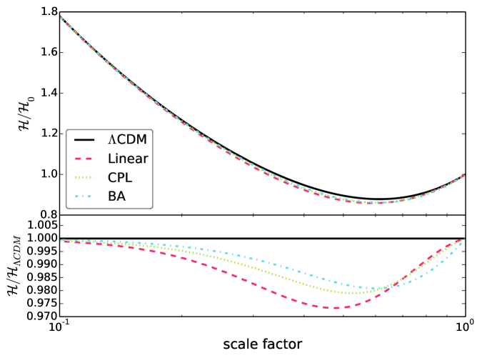
Figure 1: Evolution of the conformal Hubble parameter (${\cal H}=aH$) for the three dark energy parameterisations discussed in the text. The curves are obtained for the best-fit values given by the joint JLA + BAO analysis.

4.1 SNe Ia

For the first cosmological test we will employ the most recent SNe Ia catalog available, the JLA (acronym for Joint Lightcurve Analysis) described in [17]. Given the same trend as using the full catalog itself, we employ here the catalog with a binned sample data described in Table 1 which consists of $N_{\text{JLA}}=31$ SNe Ia events distributed over the redshift interval $0.01<z<1.3$. The statistical analysis of the this binned data lies in the definition of the modulus distance:

$$\mu(z_{i},\mu_{0})=5\log_{10}\left[d_{L}(z_{i},\Omega_{m};w_{0},w_{1})\right]+\mu_{0},$$ (4.1)

where

$$d_{L}(z,\Omega_{m};w_{0},w_{1})=(1+z)\int_{0}^{z}{d\tilde{z}E^{-1}(\tilde{z},\Omega_{m};w_{0},w_{1})},$$ (4.2)

is the Hubble free luminosity distance with $E=H(z)/H_{0}$ and ($w_{0}$, $w_{1}$) are the free parameters of the model. The best fit values are obtained by minimizing the quantity

$$\chi_{\text{SN}_{\text{JLA}}}^{2}=\sum^{N_{\text{JLA}}}_{i=1}{\frac{\left[\mu(z_{i},\Omega_{m};\mu_{0},w_{0},w_{1})-\mu_{\text{obs}}(z_{i})\right]^{2}}{\sigma^{2}_{\mu,i}}},$$ (4.3)

where the $\sigma^{2}_{\mu,i}$ are the measurements errors.

4.2 Baryon acoustic oscillations

The sample of BAO measurements used in this analysis is described in [38, 39, 40]. Before proceeding to the statistical analysis of these data, we define the ratio

$$d_{z}\equiv\frac{r_{s}(z_{d})}{D_{V}(z)},$$ (4.4)

where $r_{s}(z_{d})$ is the comoving sound horizon at the drag epoch

$$r_{s}(z_{d})=\frac{c}{H_{0}}\int_{z_{d}}^{\infty}\frac{c_{s}(z)}{E(z)}\mathrm{d}z\;,$$ (4.5)

with $c$ being the light velocity, $c_{s}$ the sound speed and $z_{d}$ the redshift of the drag epoch. By definition the dilation scale $D_{V}(z)$ is

$$D_{V}(z,\Omega_{m};w_{0},w_{1})=\left[(1+z)^{2}D_{A}^{2}\frac{c\,z}{H(z,\Omega_{m};w_{0},w_{1})}\right]^{1/3},$$ (4.6)

where $D_{A}$ is the angular diameter distance:

$$D_{A}(z,\Omega_{m};w_{0},w_{1})=\frac{1}{1+z}\int_{0}^{z}\frac{c\,\mathrm{d}z^{\prime}}{H(z^{\prime},\Omega_{m};w_{0},w_{1})}\;.$$ (4.7)

Through the comoving sound horizon, the distance ratio $d_{z}$ is related to the expansion parameter $h$ (defined such that $H\doteq 100h$ km/s/Mpc) and the physical densities $\Omega_{m}$ and $\Omega_{b}$. Specifically, we have

$$r_{s}(z_{d})=153.5\left(\frac{\Omega_{b}h^{2}}{0.02273}\right)^{-0.134}\left(\frac{\Omega_{m}h^{2}}{0.1326}\right)^{-0.255}\;\mathrm{Mpc},\;$$ (4.8)

with $\Omega_{b}=0.045\pm 0.00054$.

The $\chi^{2}$ function for the BAO data is defined as:

$$\chi^{2}_{\mathrm{BAO}}(\boldsymbol{\theta})=\mathbf{X}^{T}_{\mathbf{BAO}}\mathbf{C}^{-1}_{\mathbf{BAO}}\mathbf{X}_{\mathbf{BAO}},$$ (4.9)

where $\mathbf{X}_{\mathbf{BAO}}$ is given as

$$\mathbf{X_{BAO}}=\left(\begin{array}[]{c}\frac{r_{s}(z_{d})}{D_{V}(0.106,\Omega_{m};w_{0},w_{1}})-0.336\\ \frac{r_{s}(z_{d})}{D_{V}(0.35,\Omega_{m};w_{0},w_{1}})-0.1126\\ \frac{r_{s}(z_{d})}{D_{V}(0.57,\Omega_{m};w_{0},w_{1}})-0.07315\\ \end{array}\right)\;,$$ (4.10)

and

$$\mathbf{C}^{-1}_{\textbf{BAO}}=\text{diag}(4444,215156,721487),$$ (4.11)

In order to determine the best fit values of the parameters $w_{0}$ and $w_{1}$ for our three parameterisations discussed above, we will employ the maximum likelihood method, where the total likelihood for joint data analysis is expressed as the sum of each dataset, i.e.,

$$\chi_{\text{Total}}^{2}=\chi_{\text{SN}_{\text{JLA}}}^{2}+\chi^{2}_{\text{BAO}}.$$ (4.12)

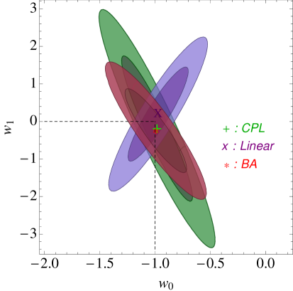
Figure 2: Comparison between three dark energy parameterisations at 1$\sigma$ and 2$\sigma$ confidence contours tested with JLA supernovae binned data sample. The dashed line represent the $\Lambda$CDM model. The best fit points for each model are represented by a ‘green plus sign’ in the case of the CPL model, a ‘purple x sign’ in the case of the Linear model and ‘red star sign’ for the BA model [41].

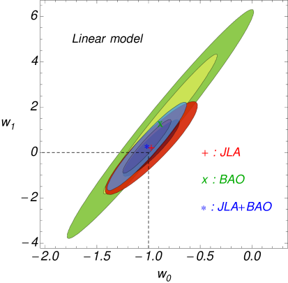
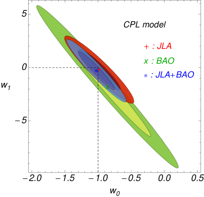
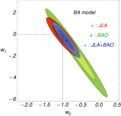
Figure 3: 1 and 2$\sigma$ confidence contours for the parameterisations discussed in the text. Constraints from the JLA supernovae binned data are represented by the red region whereas the BAO high-$z$ sample with ($z=0.106,0.35,0.57$) are the green region. The combined JLA+BAO bounds are represented by the blue region. The point where the dashed lines cross indicates the $\Lambda$CDM model. The best fit points for each dataset are represented by a ‘red plus sign’ in the case of the JLA sample, a ‘green x sign’ in the case of the BAO sample and ‘blue star sign’ for the combined JLA+BAO sample.

Table 2: Parameterisation models and data. Column. 1: Models; columns 2 - 3 - 4: best fit values of $w_{0}$ and $w_{1}$ using JLA supernovae binned and BAO samples; column. 5: $d_{\sigma}$ with respect to the $\Lambda$CDM model using (4.13).

$\mathrm{Model}$	$\mathrm{Best\;fit\;parameters\;(w_{0},w_{1})}$			$d_{\sigma}^{\mathrm{Model-\Lambda}}$
	JLA binned sample	BAO sample	JLA+BAO samples	JLA	BAO	JLA+BAO
Linear	$-0.973\pm 0.032$, $0.195\pm 0.685$	$-0.885\pm 0.133$, $1.258\pm 4.139$	$-1.015\pm 0.024$, $0.271\pm 0.616$	$0.05$	$0.73$	$0.86$
CPL	$-0.982\pm 0.045$, $-0.190\pm 1.632$	$-0.858\pm 0.187$, $-1.797\pm 9.441$	$-1.024\pm 0.033$, $-0.283\pm 1.419$	$0.03$	$0.73$	$0.83$
BA	$-0.993\pm 0.034$, $-0.068\pm 0.388$	$-0.621\pm 0.119$, $-1.707\pm 2.731$	$-0.892\pm 0.024$, $-0.535\pm 0.450$	$0.02$	$0.60$	$0.80$

4.3 Background analysis: results

For our background analysis we include the Planck data [21], were the selected priors for $\Omega_{m}$ and $\Omega_{b}$ are obtained from a forecast of CMB observations with this astrophysical mission. In Figure 2 we show the confidence contours for the three parameterisations using only the JLA data set. The results of the joint SNe Ia + BAO analysis are shown in Figure 3 where we observe a clear compatibility with the $\Lambda$CDM model. To compare the tension [35] among datasets, we compute the so-called $\sigma$-distance, $d_{\sigma}$, between the best fit points of each parameterisation and of the $\Lambda$CDM model obtained from the SNe Ia, BAO and the total SNe Ia + BAO analyses. Following [42], the $\sigma$-distance is calculated by solving

$$1-\Gamma(1,|\Delta\chi_{\sigma}^{2}/2|)/\Gamma(1)=\mathrm{erf}(d_{\sigma}/\sqrt{2}),$$ (4.13)

where $\Gamma$ and $\mathrm{erf}$ are the Gamma and the error functions, respectively, and $\Delta{\chi_{\sigma}^{2}}(w_{0})=\chi_{\text{Total}}^{2}(w_{0_{\text{JLA + BAO}}})-\chi_{\text{Total}}^{2}(w_{0_{\text{JLA}}})$. We follow the same rule for $w_{1}$.

The tension between probes seems to be reduced when we use the BA parameterisation. From Table 2 we also observe that the best fit obtained by using the BA case is in better agreement with $\Lambda$CDM, around 1% of difference than using the CPL case.

5 Perturbative Analysis

Apart from the evolution of the homogeneous part of the dark energy parameterisations, the linear perturbations are indeed a substantial analysis to understand their evolution. In order to describe their dynamics when a scalar field is included, let us write the Einstein equations as

$$R_{\mu\nu}-\frac{1}{2}g_{\mu\nu}R=8\pi GT^{b}_{\mu\nu}+\phi_{;\mu}\phi_{;\nu}-\frac{1}{2}g_{\mu\nu}\phi_{,a}\phi^{a}_{,}+g_{\mu\nu}V,$$ (5.1)

which preserves the conservation equation

$${T^{\mu\nu}_{b}}_{;\mu}=0,$$ (5.2)

with the Klein-Gordon equation:

$$\Box\phi=-V_{\phi},$$ (5.3)

where $\phi^{2}=8\pi G\psi^{2}$ and $V=8\pi GU$. Rewriting Eq.(5.1) as

$$R_{\mu\nu}=8\pi G\left(T_{\mu\nu}^{b}-\frac{1}{2}g_{\mu\nu}T^{b}\right)+\phi_{,\mu}\phi_{,\nu}-g_{\mu\nu}V,$$ (5.4)

we can perturbed to obtain

$$\delta R_{\mu\nu} = 8\pi G\left(\delta T_{\mu\nu}^{b}-\frac{1}{2}h_{\mu\nu}T^{b}-\frac{1}{2}g_{\mu\nu}\delta T^{b}\right)+\left(\delta\phi_{,\mu}\phi_{,\nu}+\phi_{,\mu}\delta\phi_{,\nu}\right)-h_{\mu\nu}V-g_{\mu\nu}\delta V.\quad$$ (5.5)

If we consider the component $\mu=0$, $\nu=0$, we obtain, with the synchronous coordinate condition,

$$\frac{1}{2}\ddot{h}+\left(\frac{\dot{a}}{a}\right)\dot{h}=4\pi G\,\delta\rho_{m}+2\dot{\phi}\,\delta\dot{\phi}-V_{\phi}\,\delta\phi.$$ (5.6)

The variation of the energy-momentum tensor Eq.(5.2) sets the following

$$\delta\left(T_{b;\mu}^{\mu\nu}\right)=0,\quad\rightarrow\quad\dot{\delta}=\frac{\dot{h}}{2}.$$ (5.7)

Using this latter and assuming $\delta=\delta\rho_{m}/\rho_{m}$, $8\pi G\rho_{m}=3H_{0}^{2}\Omega_{m}/a^{3}$, $\delta\phi=\nu$ in Eq.(5.6) we have

$$\ddot{\delta}+2\left(\frac{\dot{a}}{a}\right)\dot{\delta}-\frac{3}{2}H_{0}^{2}\Omega_{m}a^{-3}\delta=2\dot{\phi}\dot{\nu}-V_{\phi}\nu.$$ (5.8)

Now, the variation of the D’Alembert operator of the scalar field Eq.(5.3) can be computed as

$$\delta(\Box\phi)=-\delta V_{\phi}=-V_{\phi\phi}\nu,$$ (5.9)

then

$$\delta(\Box\phi) = \delta\left[g^{\rho\sigma}\left(\phi_{,\rho,\sigma}-\Gamma_{\rho\sigma}^{\lambda}\phi_{,\lambda}\right)\right]$$ (5.10)

$$= -h^{\rho\sigma}\left(\phi_{,\rho,\sigma}-\Gamma_{\rho\sigma}^{\lambda}\phi_{,\lambda}\right)+g^{\rho\sigma}\left(\delta\phi_{,\rho,\sigma}-\Gamma_{\rho\sigma}^{\lambda}\delta\phi_{,\lambda}-\chi_{\rho\sigma}^{\lambda}\phi_{,\lambda}\right).$$

Using Eq.(5.9) and the component when $\lambda=0$ we finally have

$$\ddot{\nu}+3\left(\frac{\dot{a}}{a}\right)\dot{\nu}+\left(\frac{k^{2}}{a^{2}}\right)\nu-\left(\frac{\dot{h}}{2}\right)\dot{\phi}=-V_{\phi\phi}\nu.$$ (5.11)

Also, as we did for Eq.(5.8) we can rewrite Eq.(5.11) as

$$\ddot{\nu}+3\left(\frac{\dot{a}}{a}\right)\dot{\nu}+\left(\frac{k^{2}}{a^{2}}+V_{\phi\phi}\right)\nu=\dot{\delta}\dot{\phi}.$$ (5.12)

Finally, taking $\dot{\delta}=\dot{a}\delta^{\prime}$, where the prime denotes derivatives with respect to the scale factor, we can compute the following perturbation equations for a scalar field with a specific set of $\dot{\phi}$ and $V_{\phi}$

$$\delta^{\prime\prime}+\left(\frac{2}{a}+\frac{{\cal H}^{\prime}}{{\cal H}}\right)\delta^{\prime}-\frac{3}{2}\frac{H_{0}^{2}\Omega_{m}}{{\cal H}^{2}a^{3}}\delta=2\phi^{\prime}\nu^{\prime}-\frac{V_{\phi}}{{\cal H}^{2}}\nu,$$ (5.13)

$$\nu^{\prime\prime}+\left(\frac{3}{a}+\frac{{\cal H}^{\prime}}{{\cal H}}\right)\nu^{\prime}+\left[\left(\frac{k}{a}\right)^{2}+V_{\phi\phi}\right]\frac{\nu}{{\cal H}^{2}}=\phi^{\prime}\delta^{\prime},\quad\quad$$ (5.14)

where ${\cal H}=\dot{a}$ and $\phi^{\prime}=\dot{\phi}/{\cal H}.$

5.1 Solutions of linear perturbations and CMB analysis

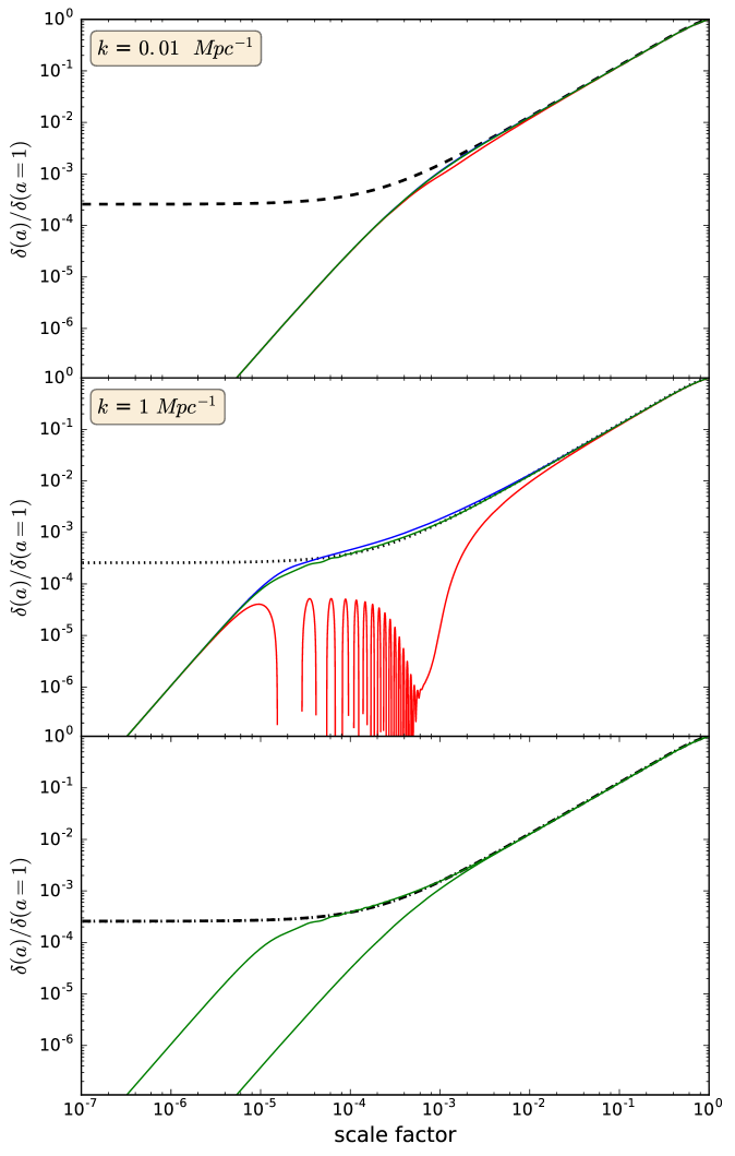
Figure 4: $k$ modes for the CPL parameterisation. Top: The mode $k=0.01Mpc^{-1}$ of the $\delta$ solution of (5.14) in black-dashed, compared with the output of the modified CAMB for cold dark matter ($\delta_{c}$ in blue), baryons ($\delta_{b}$ in red) and all matter ($\delta_{m}$ in green). Middle: The same for the mode $k=1$ ($\delta$ in black-dotted). Bottom: The two $\delta$ modes are undistinguishable and overlap to the CAMB solutions of $\delta_{m}$ after the recombination era. For brevity, we only show the behaviour for CPL model since the results for the other two parameterisations are essentially the same.

In the attempt to account for a complete treatment of the linear evolution of perturbations from the entry in the horizon of perturbations produced by inflation until today for each scale, we modified the Boltzmann code named CAMB [29], that solves numerically the fluid equations following [43]:

$$\delta_{i}^{\prime}+3{\cal H}(\hat{c}_{s,i}^{2}-w_{i})(\delta_{i}+3{\cal H}(1+w_{i})v_{i}/k)+(1+w_{i})kv_{i}+3{\cal H}w^{\prime}_{i}v_{i}/k=-3(1+w_{i})h^{\prime}$$ (5.15)

$$v_{i}^{\prime}+{\cal H}(1-3\hat{c}_{s,i}^{2})v_{i}=k\hat{c}_{s,i}^{2}\ \delta_{i}/(1+w_{i})\,$$ (5.16)

where derivatives are respect the conformal time, ${\cal H}$ is the conformal Hubble parameter, $v_{i}$ is the velocity, $w_{i}\equiv p_{i}/\rho_{i}$, $h^{\prime}=(\delta a/a)^{\prime}$, and $\hat{c}_{s}^{2}$ is the sound speed evaluated in the frame co-moving with dark energy ($\hat{c_{s}}=1$ for quintessence).

In order to avoid the crossing instability problem at the phantom divide line, i.e. $w=-1$, the CAMB code provides a module that implements the Parameterized Post-Friedmann (PPF) approach [30] for the CPL model. We modified it to also include the Linear and BA parameterisations. The advantage of this approach is to replace the condition on the dark energy pressure perturbation with a relationship between the momentum density of this dark component and that of the other components on the large scales, providing a well-controlled approximation for any model where the energy and momentum of the dark energy are separately conserved.

The solution of (5.8) and (5.11) are compared with the solution of (5.13) and (5.14) for different modes, $k=0.01\,h$Mpc^-1 and $k=1\,h$Mpc^-1, and shown in Figure 4 for the CPL case. We start the computation of (5.8) and (5.11) inside the radiation era at $a=10^{-7}$ with $\dot{\delta}=\delta\dot{a}/(a+a_{eq}/1.5)$, where $a_{eq}$ is the scale factor at radiation-matter equivalence [20], and, concordantly, we consider the radiation term contribution in the Friedmann equation. In this figure we see that the evolution of $\delta(a)$ is scale invariant for the parametrisations here considered. Qualitatively, the scalar field undergo damped oscillations for scales $k>a^{2}V_{\phi\phi}$. On these scales the scalar field will not contribute to the total gravitational potential and can be approximated as homogeneous. The difference of the solutions at early time, occurs because CAMB takes into account the entrance of the perturbations at the horizon scale. On the contrary, for eqs (5.8) and (5.11), we set the initial conditions immediately inside the horizon scale at $a=10^{-7}$, when, actually, the perturbations at scales $k=1\,h$Mpc^-1 and $k=0.01\,h$Mpc^-1 have not entered inside the horizon yet. Accordingly, Figure 4 shows that the solutions overlap after the perturbations have entered in the horizon (in CAMB), and not before.

The comparison of the results obtained from CAMB for the different dark energy parametrizations are shown in Figure 5. The CMB power spectra of our models with respect to the $\Lambda$CDM cosmology are shown in the upper panel. All the models share the same $\log$ power of the primordial curvature perturbations ln$(10^{10}A_{s})=3.09$ and the same scalar spectrum index $n_{s}=0.966$, with $k_{0}=0.05$ Mpc^-1 as indicated by [21]. Fixing the set of parameters by the SNe Ia constraints for each model, the discrepancies from the $\Lambda$CDM scenario favor the BA parameterisation. A finest future analysis could also consider the employment of the code COSMOMC [44] that provides a joint analysis of background and perturbation exploring a large dimensional space of parameters.

Finally, as mentioned earlier, the $\delta(a)$ evolution is scale-invariant. Therefore, we can have a complete description of the growth rate of structure, defined as $f_{\Omega}=\frac{d\ln{\delta}}{d\ln{a}}$, by considering a single mode. In the bottom panel of Figure 5, it is shown that the variations with respect to the different models do not exceed $\sim 2.5\%$ at $z=0$.

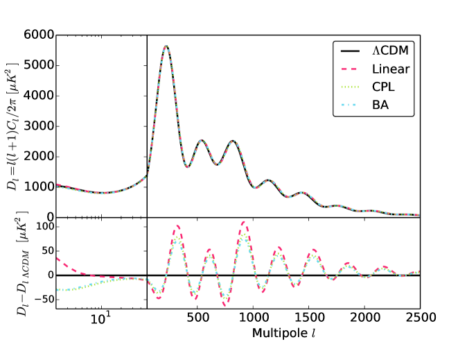
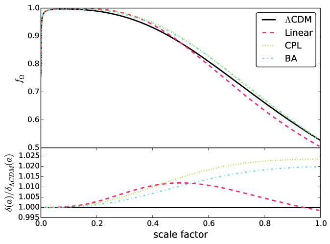
Figure 5: Top: Linear analysis using PPF. The CMB $C^{TT}_{l}$ power spectrum versus multipole moment $l$ using the best fit values obtained for each dark energy parameterisation using the combined JLA+BAO data set. Bottom: The evolution of $f_{\Omega}$ and $\delta(a)$ for each model.

6 Non linear power spectrum

In this section we estimate the non-linear contribution of the $w(z)$ parameterisations to the matter power spectrum. The aim here is to detect any observational signature that may distinguish among these models. Such contribution can be derived in a straightforward way by performing time expansive numerical simulations. However, this is not necessary. A common approach in the prediction of the $P(k)$ is to compute the non linearities using the Halofit recipe [31] revised in [32]. In [45], it was introduced the HMcode, a fit of the Halo model [46] on the Coyote suite simulations [47] including also the effect of baryons physics as quantified in [48], that implemented star formation, supernovae and active galactic nucleus feedback. Despite these methods are built on simulations of models including $w=const.$ only, they are employed for $w=w(a)$ models [21], by entering an evident bias in the forecasts.

In Ref. [33], it was found a spectral equivalence between $w=w(a)$ models and $w=const$, that drastically simplifies the task to find a universal Halo model. Previous authors [49] had shown how spectral predictions for constant–$w$ models at $z=0$ can also be used to fit spectra of CPL cosmologies with a precision $\sim 1\%$. To meet such precision at non-zero redshift, a new technique is needed, that it was defined in [33] and tested for several models [33, 50], both through purely gravitational simulations and through simulations including baryon physics [51]. Recently, in [34] it was described a public package called PKequal, that extends both Halofit and Coyote suite from $w=const$ to CPL models. In this work, we modified the PKequal code in order to also include the Linear and BA cases and chose to extend the predictions of the code described in [47]. The results are shown in Figure 6. We observe that most of the discrepancies is due to the linear evolution, while the non-linear contribution is almost the same for all the scales. Indeed the $P(k)$ differs between the models according to the $\delta(a)$ evolution at $z=0$ (see Figure 6). Clearly, the current uncertainties on the cosmological parameters do not allow to discriminate between the parameterisation models. It is expected that future weak lensing surveys that aim to distinguish matter distribution at $1\%$ level, e.g. Euclid [52], will be able to discriminate time-dependent dark energy parameterisations from the standard $\Lambda$CDM model using the observables discussed in this analysis.

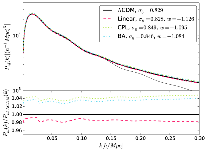
Figure 6: Non linear power spectrum derived using the PKequal package, as discussed in the text. $\sigma_{8}$ values are computed on the linear spectra and the w values are the equivalent w-constant models that reproduce the non linear spectra for every model, following [33, 34]. The thin line represents the linear matter power spectrum predicted by the $\Lambda$CDM model.

7 Conclusions

We have studied three dark energy parameterisations with two free parameters (Linear, CPL and BA), which make suitable for fitting the current JLA, BAO and the combination of these datasets. By using these models, it was possible to set the dynamics of the dark energy in a scalar field representation. In Table 2 it was reported the best-fit parameters for each model using the current cosmological data. Also, it is important to remark that we have presented a complete treatment of the linear evolution of perturbations from the entry of perturbations produced by inflation in the horizon until today. We have calculated the numerical perturbations for each parametrisation and shown that the differences of the growth factors for extreme values of $k$ are almost negligible. Furthermore, using a suitable spectral equivalence, we have shown that the non-linear contribution of the selected dark energy parameterisations to the matter power spectra is almost the same for all scales of interest. Finally, we have observed that, for the current uncertainties on the cosmological parameters, the power spectrum for our three selected parameterisations is indistinguishable from the one predicted by the standard model. We expect the next generation of cosmology experiments to be able to distinguish between time-dependent $w(z)$ models and the standard $\Lambda$CDM cosmology using the observables discussed in the present analysis.

References

- [1] S. Weinberg, astro-ph/0005265.
- [2] V. Sahni and A. A. Starobinsky, Int. J. Mod. Phys. D 9, 373 (2000)
- [3] T. Padmanabhan, Phys. Rept. 380, 235 (2003)
- [4] P. J. E. Peebles and B. Ratra, Rev. Mod. Phys. 75, 559 (2003)
- [5] E. J. Copeland, M. Sami and S. Tsujikawa, Int. J. Mod. Phys. D 15, 1753 (2006)
- [6] R. R. Caldwell, Phys. Lett. B 545, 23 (2002)
- [7] S. M. Carroll, M. Hoffman and M. Trodden, Phys. Rev. D 68, 023509 (2003)
- [8] J. S. Alcaniz, Phys. Rev. D 69, 083521 (2004)
- [9] J. A. S. Lima and J. S. Alcaniz, Phys. Lett. B 600, 191 (2004)
- [10] J. A. S. Lima, J. V. Cunha and J. S. Alcaniz, Phys. Rev. D 68, 023510 (2003) [astro-ph/0303388].
- [11] L. Feng and T. Lu, JCAP 1111, 034 (2011) [arXiv:1203.1784 [astro-ph.CO]].
- [12] H. Stefancic, J. Phys. Conf. Ser. 39, 182 (2006) [astro-ph/0512023].
- [13] H. K. Jassal, J. S. Bagla and T. Padmanabhan, Mon. Not. Roy. Astron. Soc. 356, L11 (2005) [astro-ph/0404378].
- [14] Y. Wang, Phys. Rev. D 77, 123525 (2008) [arXiv:0803.4295 [astro-ph]].
- [15] Y. Wang and M. Tegmark, Phys. Rev. D 71, 103513 (2005) [astro-ph/0501351].
- [16] E. M. Barboza, J. S. Alcaniz, Z.-H. Zhu and R. Silva, Phys. Rev. D 80, 043521 (2009) [arXiv:0905.4052 [astro-ph.CO]].
- [17] M. Betoule et al. [SDSS Collaboration], Astron. Astrophys. 568, A22 (2014) [arXiv:1401.4064 [astro-ph.CO]].
- [18] B. Santos, N. C. Devi and J. S. Alcaniz, arXiv:1603.06563 [astro-ph.CO].
- [19] N. G. Busca et al., Astron. Astrophys. 552, A96 (2013) [arXiv:1211.2616 [astro-ph.CO]].
- [20] P. J. E. Peebles, The large-scale structure of the universe, Princeton University Press, 1980
- [21] P. A. R. Ade et al. [Planck Collaboration], arXiv:1502.01589 [astro-ph.CO].
- [22] M. Hicken, W. M. Wood-Vasey, S. Blondin, P. Challis, S. Jha, P. L. Kelly, A. Rest and R. P. Kirshner, Astrophys. J. 700, 1097 (2009) [arXiv:0901.4804 [astro-ph.CO]].
- [23] D. Stern, R. Jimenez, L. Verde, M. Kamionkowski and S. A. Stanford, JCAP 1002, 008 (2010) [arXiv:0907.3149 [astro-ph.CO]].
- [24] A. R. Cooray and D. Huterer, Astrophys. J. 513, L95 (1999)
- [25] Weller, J. and Albrecht, A., Phys. Rev Lett. 86, 1939 (2001)
- [26] M. Chavallier and D. Polarski, Int. J. Mod. Phys. D10, 213 (2001)
- [27] E. V. Linder, Phys. Rev Lett. 90, 091301 (2003)
- [28] E. M. Barboza, Jr. and J. S. Alcaniz, Phys. Lett. B 666, 415 (2008) [arXiv:0805.1713 [astro-ph]].
- [29] A. Lewis, A. Challinor, A. Lasenby, ApJ 538, 473 (2000) [arXiv:astro-ph/9911177].
- [30] W. Hu,/ Phys. Rev. D 77, 103524 (2008) [arXiv:0801.2433 [astro-ph]]. W. Fang, W. Hu and A. Lewis, Phys. Rev. D 78, 087303 (2008) [arXiv:0808.3125 [astro-ph]].
- [31] R. E. Smith, J. A. Peacock, A. Jenkins, S. D. M. White, C. S. Frenk, F. R. Pearce, P. A. Thomas, G. Efstathiou, and H. M. P. Couchman, MNRAS 341, (2003)
- [32] R. Takahashi, M. Sato, T. Nishimichi, A. Taruya, and M. Oguri, ApJ 761, 152 (2012)
- [33] L. Casarini, A. V. Macció, and S. A. Bonometto, J. Cosmology Astropart. Phys., 3, 14 (2009)
- [34] L. Casarini, S. A. Bonometto, E. Tessarotto, and P.-S. Corasaniti, arXiv:1601.07230 [astro-ph.CO]
- [35] C. Escamilla-Rivera, R. Lazkoz, V. Salzano and I. Sendra, JCAP 1109, 003 (2011) [arXiv:1103.2386 [astro-ph.CO]].
- [36] E. M. Barboza, B. Santos, F. E. M. Costa and J. S. Alcaniz, Phys. Rev. D 85, 107304 (2012) [arXiv:1107.2628 [astro-ph.CO]].
- [37] Y. Wang and M. Tegmark, Phys. Rev. Lett. 92, 241302 (2004)
- [38] F. Beutler et al., Mon. Not. Roy. Astron. Soc. 416, 3017 (2011) [arXiv:1106.3366 [astro-ph.CO]].
- [39] X. Xu, N. Padmanabhan, D. J. Eisenstein, K. T. Mehta and A. J. Cuesta, Mon. Not. Roy. Astron. Soc. 427, 2146 (2012) [arXiv:1202.0091 [astro-ph.CO]].
- [40] L. Anderson et al. [BOSS Collaboration], Mon. Not. Roy. Astron. Soc. 441, no. 1, 24 (2014) [arXiv:1312.4877 [astro-ph.CO]].
- [41] C. Escamilla-Rivera, Galaxies 4, 8 (2016) doi:10.3390/galaxies4030008 [arXiv:1605.02702 [astro-ph.CO]].
- [42] Press W.H, et.al. Numerical Recipes. 1994. Cambridge Press.
- [43] J. Weller and A. M Lewis, MNRAS 346, 987 (2004) [arXiv:astro-ph/0307104]
- [44] A. Lewis and S. Bridle, Phys. Rev. D, 66, 103511 (2002) [arXiv:astro-ph/0205436]
- [45] A. J. Mead, J. A. Peacock, C. Heymans, S. Joudaki, and A. F. Heavens, MNRAS, 454, 1958 (2015)
- [46] U. Seljak, MNRAS, 318, 203 (2000). J. A. Peacock and R. E. Smith, MNRAS, 318, 1144 (2000). A. Cooray and R. Sheth, Phys. Rep., 372, 1 (2002)
- [47] K. Heitmann, E. Lawrence, J. Kwan, S. Habib, and D. Higdon, ApJ 780, 111 (2014)
- [48] M. P. van Daalen, J. Schaye, C. M. Booth, and C. Dalla Vecchia, MNRAS, 415, 3649 (2011)
- [49] M. J. Francis, G. F. Lewis, and E. V. Linder, MNRAS 380, 1079 (2007)
- [50] L. Casarini. J. Cosmology Astropart. Phys., 8, 5 (2010)
- [51] L. Casarini, A. V. Macció, S. A. Bonometto, and G. S. Stinson MNRAS, 412, 911 (2011)
- [52] A. Refregier et al., Euclid Imaging Consortium - Euclid Imaging Consortium Science Book, arXiv:1001.006; R. Laureijs et al., Euclid collaboration - Euclid Definition Study Report, arXiv:1110.3193; L. Amendola, S. Appleby, D. Bacon, et al., Living Rev. Relativity 16, 6 (2013); http://sci.esa.int/euclid/.