Abstract

To bridge the gap between high and low fidelity numerical modeling tools for vertical-axis (or cross-flow) turbines (VATs or CFTs), an actuator line model (ALM) was developed and validated for both a high and a medium solidity vertical-axis turbine at rotor diameter Reynolds numbers $Re_{D}\sim 10^{6}$. The ALM is a combination of classical blade element theory and Navier–Stokes based flow models, and in this study both $k$–$\epsilon$ Reynolds-averaged Navier–Stokes (RANS) and Smagorinsky large eddy simulation (LES) turbulence models were tested using the open-source OpenFOAM computational fluid dynamics framework. The RANS models were able to be run on coarse grids while still providing good convergence behavior in terms of the mean power coefficient, and also approximately four orders of magnitude reduction in computational expense compared with 3-D blade-resolved RANS simulations. Submodels for dynamic stall, end effects, added mass, and flow curvature were implemented, resulting in reasonable performance predictions for the high solidity rotor, more discrepancies for the medium solidity rotor, and overprediction for both cases at high tip speed ratio. The wake results showed that the ALM was able to capture some of the important flow features that contribute to VAT’s relatively fast wake recovery—a large improvement over the conventional actuator disk model. The mean flow field was better realized with the LES, which still represented a computational savings of two orders of magnitude compared with 3-D blade-resolved RANS, though vortex breakdown and subsequent turbulence generation appeared to be underpredicted, which necessitates further investigation of optimal subgrid scale modeling.

xx 1 1 Preprint uploaded XXXXXX Received: date; Accepted: date; Published: date Actuator line modeling of vertical-axis turbines Peter Bachant ¹, Anders Goude ² and Martin Wosnik ^1,* Peter Bachant, Anders Goude and Martin Wosnik Correspondence: martin.wosnik@unh.edu

1 Introduction

Vertical-axis (cross-flow) turbines (VATs or CFTs) were the subject of significant research and development in the 1970s through the 1990s by groups like Sandia National Labs in the US Sutherland et al. (2012) and the National Research Council of Canada Paraschivoiu (2002). Despite minor commercial success for large scale onshore wind applications, vertical-axis turbines were virtually abandoned in favor of horizontal-axis (or axial-flow) turbines, as they generally are more efficient and do not encounter the high levels of fatigue loading that VATs do. Today, however, there is renewed interest in VATs for marine hydrokinetic (MHK) applications Ocean Renewable Power Company (2012), offshore floating wind farms Paulsen et al. (2011); Sandia National Laboratories (2012); Dodd (2014), and smaller scale, tightly spaced wind farms Dabiri (2011); Kinzel et al. (2012), thanks to their relatively faster wake recovery.

The mean near-wake structure of vertical-axis turbine has been shown to be largely dominated by the effects of tip vortex shedding, which induces levels of recovery due to vertical advection significantly larger than those from turbulent fluctuations Bachant and Wosnik (2015)—an effect not seen in axial-flow or horizontal-axis turbine (AFT or HAT) wakes. As interest shifts to designing and analyzing arrays of VATs, it is necessary to determine the effectiveness of various numerical modeling techniques to replicate VAT near-wake dynamics, such that wake recovery is accurately predicted, leading to accurate assessment of optimal array spacing.

Reynolds-averaged Navier–Stokes (RANS) turbulence models computed on 3-D body-fitted (blade-resolved) grids can do a good job predicting the mean performance and near-wake structure of a VAT, though their effectiveness depends on the turbulence model applied Bachant and Wosnik (2016); Lam and Peng (2016); Alaimo et al. (2015); Boudreau and Dumas (2017); Marsh et al. (2015). However, 3-D blade-resolved RANS presents a huge computational expense—on the order of 1,000 CPU hours per simulated second with contemporary hardware—since it must resolve fine details of the blade boundary layers, which will preclude its use for array analysis until the availability of computing power increases sufficiently. It is therefore necessary to explore simpler models that can predict the turbine loading and flow field with acceptable fidelity, but that are economical enough to not require high performance computing, at least for individual devices.

For analyzing turbine arrays, it is desirable to retain a Navier–Stokes description of the flow field—in contrast to, e.g., momentum or potential flow vortex models—to capture the effects of nonlinear advection and turbulent transport. However, rather than resolving the fine details in the blade boundary layers, an actuator-type model for parameterizing the turbine loading may be employed, which dramatically drives down computational expense. As shown in Bachant and Wosnik (2015), the conventional uniform actuator disk is not a good candidate for a cross-flow turbine wake generator, never mind the fact that it does not typically compute performance predictions.

Actuator line modeling (ALM), originally developed by Sorensen and Shen Sørensen and Shen (2002), is an unsteady method that tracks blade element locations, and has become popular for modeling axial-flow or horizontal-axis turbines, and has been shown in blind tests to be competitive with blade-resolved CFD Krogstad and Eriksen (2013); Pierella et al. (2014). The ALM combined with large eddy simulation (LES) has become the state-of-the-art for modeling entire wind farms Archer et al. (2013); Churchfield et al. (2012); Sørensen et al. (2015); Fleming et al. (2013, 2014). Like other blade element techniques, the effectiveness of the ALM for AFTs is in part due to the quasi-steady nature of the flow in the blade reference frame, and the relatively rare occurrence of stall. Note that a similar method can be used with the Navier–Stokes equations in vorticity–velocity form Scheurich et al. (2011), which may be more efficient when vorticity is confined to a relatively small fraction of the domain, e.g., for a standalone turbine with a uniform laminar inflow.

The ALM has been previously used to model a very low Reynolds number (based on rotor diameter, $Re_{D}\sim 10^{4}$) 2-D cross-flow turbine experiment in a flume using large eddy simulation (LES) Shamsoddin and Porté-Agel (2014). Performance predictions for this case were not reported, but the ALM was shown to be more effective at postdicting the wake characteristics measured in the experiments by Brochier et al. Brochier et al. (1986).

In this study we have developed an ALM for cross-flow turbines and embedded the model inside LES and unsteady RANS simulations, the latter of which has not yet been reported in the literature. This model was implemented within the open-source OpenFOAM CFD framework and validated against experimental data for the high solidity ($c/R=0.28$) UNH Reference Vertical-Axis Turbine (UNH-RVAT) and the medium solidity ($c/R=0.07$–$0.12$) US Department of Energy/Sandia National Labs Reference Model 2 (RM2) cross-flow turbine (at 1:6 scale), both of which are shown in Figure 1. Validation datasets for both turbines were taken from Bachant and Wosnik (2016) and Bachant et al. (2016), respectively. The turbines were modeled at $Re_{D}\sim 10^{6}$, at which experimentally measured performance and near-wake characteristics were nearly Reynolds number independent Bachant and Wosnik (2016); Bachant et al. (2016), and two orders of magnitude higher than previous ALM investigations for VATs.

Figure 1: Drawings of the turbines modeled in this study: the UNH-RVAT (left) and DOE/SNL RM2 (right).

2 Theory

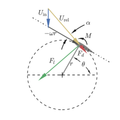
The actuator line model is based on the classical blade element theory combined with a Navier–Stokes description of the flow field. The ALM treats turbine blades as lines of blade or actuator line elements, defined by their quarter-chord location, and for which 2-D profile lift and drag coefficients are known. For each blade element, relative flow velocity $\vec{U}_{\mathrm{rel}}$ and angle of attack $\alpha$ are computed by adding the vectors of relative blade motion $-\omega r$, where $\omega$ is the rotor angular velocity and $r$ is the blade element radius, and the local inflow velocity $\vec{U}_{\mathrm{in}}$, a diagram of which is shown in Figure 2.

Figure 2: Vector diagram of velocity and forcing on a cross-flow turbine blade element. Note that the free stream velocity $U_{\infty}$ is oriented from top to bottom (identical to $U_{\mathrm{in}}$ for purely geometric calculations), the blade chord (dash-dotted line) is coincident with the tangential velocity (i.e., zero preset pitch, which would offset the geometric angle of attack $\alpha$), and the drag vector is magnified by a factor of two (approximately, relative to the lift vector) to enhance visibility.

Inflow velocity was sampled for each actuator line element at its quarter-chord location using OpenFOAM’s interpolationCellPoint class, which provides a linear weighted interpolation using cell values. This algorithm helps keep the sampled velocity “smooth” compared with using the cell values themselves, especially when elements are moving in space as they are in a turbine, since meshes will likely have a cell size on the same order as the chord length, and will move on the order of one cell length per time step.

The kinematics of a CFT are parameterized by the tip speed ratio $\lambda=\omega R/U_{\infty}$, where $R$ is the maximum rotor radius, and $U_{\infty}$ is the free stream velocity. In contrast to an AFT, which under ideal conditions can be considered a steady machine, CFT blades encounter large amplitude and rapid oscillations in angle of attack, often exceeding the rotor blades’ static stall angles in typical operation, which makes their blade loading and performance more difficult to predict. The unsteadiness can be characterized by a reduced frequency Leishman (2006)

$$k=\frac{\omega c}{2U_{\infty}},$$ (1)

which assumes the free stream velocity is constant. Unsteady effects begin to become significant for $k>0.05$, and can become dominant for $k\geq 0.2$. Note $\omega$ in the reduced frequency equation refers to the frequency of angle of attack oscillation, which is normally sinusoidal in pitching foil experiments, but is analogous to cross-flow turbine blade kinematics, i.e., the angle of attack cycle encounted by a CFT blade has a period equal to one turbine revolution.

For a VAT or CFT reduced frequency can be reformulated in terms of the tip speed ratio as

$$k=\frac{\lambda c}{2R},$$ (2)

which is then also a function of solidity or chord-to-radius ratio $c/R$. As an example, a large scale, relatively low solidity Darrieus wind turbine such as the Sandia 34 m diameter Test Bed, with an equatorial blade chord of 0.91 m Murray and Barone (2011), a reduced frequency $k=0.16$ is encountered based solely on angle of attack oscillations at $\lambda=6$. For the two turbines studied here, reduced frequencies at the tip speed ratio of peak power coefficient, $\lambda_{0}$, are 0.27 and 0.17 (based on root chord length) for the UNH-RVAT and RM2, respectively. Therefore, both cases will be inherently unsteady, with these effects dominating the UNH-RVAT’s behavior. Hence, an accurate unsteady aerodynamics model is important to predicting blade loading.

Assuming unsteady effects can be appropriately modeled, the blade element lift force, drag force, and pitching moment are calculated as

$$F_{l}=\frac{1}{2}\rho A_{\mathrm{elem}}C_{l}|\vec{U}_{\mathrm{rel}}|^{2},$$ (3)

$$F_{d}=\frac{1}{2}\rho A_{\mathrm{elem}}C_{d}|\vec{U}_{\mathrm{rel}}|^{2},$$ (4)

$$M=\frac{1}{2}\rho A_{\mathrm{elem}}cC_{m}|\vec{U}_{\mathrm{rel}}|^{2},$$ (5)

respectively, where $\rho$ is the fluid density, $A_{\mathrm{elem}}$ is the blade element planform area (span $\times$ chord), $\vec{U}_{\mathrm{rel}}$ is the local relative velocity projected onto the plane of the element profile cross-section (i.e., the spanwise component is neglected), and $C_{l}$, $C_{d}$, and $C_{m}$ are the sectional lift, drag, and pitching moment coefficients, respectively, which are linearly interpolated from a table per the local angle of attack. The forces are then projected onto the rotor coordinate system to calculate torque, overall drag, etc. Forces from the turbine shaft and blade support struts are computed in a similar way. After the force on the actuator lines from the flow is computed, it is then added to the Navier–Stokes equations as a body force or momentum source (per unit density, assuming incompressible flow):

$$\frac{\mathrm{D}\vec{u}}{\mathrm{D}t}=-\frac{1}{\rho}\nabla p+\nu\nabla^{2}\vec{u}+F_{\mathrm{turbine}}.$$ (6)

3 Static profile coefficient data

Static input foil coefficient data were taken from Sheldahl and Klimas Sheldahl and Klimas (1981)—a popular database developed for CFTs, which contains values over a wide range of Reynolds numbers. The Sheldahl and Klimas dataset has some limitations, namely that data for some foil and/or Reynolds numbers were “synthesized” numerically from other measurements. Despite its flaws, this dataset is the likely most comprehensive available with respect to variety of profiles and ranges of Reynolds numbers. Surprisingly, considering the maturity and popularity of NACA foils, data remains scarce, especially for $Re_{c}\sim 10^{5}$.

NACA 0021 coefficients were used for both turbines, despite the fact that the UNH-RVAT is constructed from NACA 0020 foils, as a NACA 0020 dataset was not available—it is assumed the small difference in foil thickness is negligible. Since pitching moment data were only available at limited Reynolds numbers, two datasets were used: The lowest for $Re_{c}\leq 3.6\times 10^{5}$ and highest $Re_{c}\geq 6.8\times 10^{5}$. For each actuator line element, blade chord Reynolds number is computed based on the sampled inflow velocity, and the static coefficients are then interpolated linearly within the database.

Each rotor’s shaft was assumed to have a drag coefficient $C_{d}=1.1$, and the blade support strut end element drag coefficients were set to 0.05, to approximate the effects of separation in the corners of the blade–strut connections.

4 Force projection

After the force on the actuator line element from the flow is calculated, it is then projected back onto the flow field as a source term in the momentum equation. To avoid instability due to steep gradients, the source term is tapered from its maximum value away from the element location by means of a spherical Gaussian function. The width of this function $\eta$ is controlled by a single parameter $\epsilon$, which is then multiplied by the actuator line element force and imparted on a cell with distance $|\vec{r}|$ from the actuator line element quarter chord location:

$$\eta=\frac{1}{\epsilon^{3}\pi^{3/2}}\exp\left[-\left(\frac{|\vec{r}|}{\epsilon}\right)^{2}\right].$$ (7)

Troldborg Troldborg (2008) proposed that the Gaussian width should be set to twice the local cell length $\Delta x$ in order to maintain numerical stability. Schito and Zasso Schito and Zasso (2014) found that a projection $\epsilon$ equal to the local mesh length was optimal. Jha et al. Jha et al. (2014) investigated the ideal projection width for HAWT blades, recommending an equivalent elliptic planform be constructed and used to calculate a spanwise $\epsilon$ distribution.

Martinez-Tossas and Meneveau Martínez-Tossas and Meneveau (2015) used a 2-D potential flow analysis to determine that the optimal projection width for a lifting surface is 14–25% of the chord length. The width due to the wake caused by the foil drag force was recommended to be on the order of the momentum thickness $\theta$, which for a bluff body or foil at large angle of attack is related to the drag coefficient ($O(1)$) by Tennekes and Lumley (1972)

$$C_{d}=2\theta/l,$$ (8)

where $l$ is a reference length, e.g., diameter for a cylinder or chord length for a foil.

Using these guidelines, three Gaussian width values were determined: one relative to the chord length, one to the mesh size, and one to the momentum thickness due to drag force. Each three were computed for all elements at each time step, and the largest was chosen for the force projection algorithm. Using this adaptive strategy, fine meshes could benefit from the increased accuracy of more concentrated momentum sources, and coarse meshes would be protected from numerical instability.

The Gaussian width due to mesh size $\epsilon_{\mathrm{mesh}}$ was determined locally on an element-wise basis by estimating the size of the cell containing the element as

$$\Delta x\approx\sqrt[3]{V_{\mathrm{cell}}},$$ (9)

where $V_{\mathrm{cell}}$ is the cell volume. To account for the possibility of non-unity aspect ratio cells, an additional factor $C_{\mathrm{mesh}}$ was introduced, giving

$$\epsilon_{\mathrm{mesh}}=2C_{\mathrm{mesh}}\Delta x.$$ (10)

$C_{\mathrm{mesh}}$ was set to 2.0 for the simulations presented here—determined by trial-and-error to provide stability on the finest grids. However, in the ALM code $C_{\mathrm{mesh}}$ is selectable at run time for each profile used.

5 Unsteady effects

In the context of a turbine—especially a cross-flow turbine—the actuator lines will encounter unsteady conditions, both in their angle of attack and relative velocity. These conditions necessitate the use of unsteady aerodynamic models to augment the static foil characteristics, both to capture the time resolved response of the attached flow loading and effects of flow acceleration, also known as added mass. Furthermore, the angles of attack encountered by a CFT blade will often be high enough to encounter dynamic stall (DS). It is therefore necessary to model both unsteady attached and detached flow to obtain accurate loading predictions.

5.1 Dynamic stall

In this study we employed a dynamic stall model developed for low mach numbers by Sheng et al. Sheng et al. (2008)—derived from the Leishman–Beddoes (LB) semi-empirical model Leishman and Beddoes (1989). This model, along with two other Leishman–Beddoes model variants, was tested for its effectiveness in cross-flow turbine conditions by Dyachuk et al. Dyachuk et al. (2014), who concluded that the Sheng et al. variant results matched most closely with experiments. In a similar study Dyachuk and Goude (2015), the Sheng et al. model also performed better than the Gormont model Gormont (1973), which inspired its adoption here for the ALM. Note that even in the absence of stall, the LB DS models still modulate foil force and moment coefficients to account for unsteadiness, which is important for the reduced frequencies of the rotors simulated here.

Before the dynamic stall subroutine is executed, the static profile data for each element is interpolated linearly based on local chord Reynolds number, which is calculated based on the detected inflow velocity for each actuator line element and the simulation’s kinematic viscosity. The profile data characteristics—static stall angle, zero-lift drag coefficient, and separation point curve fit parameters—are then recomputed each time step such that the effects of Reynolds number on the static data are included.

Inside the ALM, angle of attack is sampled from the flow field rather than calculated based on the geometric angle of attack. Therefore, the implementation of the LB DS model was such that the equivalent angle of attack $\alpha_{\mathrm{equiv}}$ was taken as the sampled rather than the lagged geometric value. A similar implementation was used by Dyachuk et al. Dyachuk et al. (2015) inside a vortex model.

5.2 Added mass

A correction for added mass effects, or the effects due to accelerating the fluid, was taken from Strickland et al. Strickland et al. (1981), which was derived by considering a pitching flat plate in potential flow. In the blade element coordinate system, the normal and chordwise (pointing from trailing to leading edge, which is opposite the $x$-direction used by Strickland et al.) coefficients due to added mass are

$$C_{n_{\mathrm{AM}}}=-\frac{\pi c\dot{U_{n}}}{8|U_{\mathrm{rel}}|^{2}},$$ (11)

and

$$C_{c_{\mathrm{AM}}}=\frac{\pi c\dot{\alpha}U_{n}}{8|U_{\mathrm{rel}}|^{2}},$$ (12)

respectively, where $U_{n}$ is the normal component of the relative velocity, and dotted variables indicate time derivatives, which were calculated using a simple first order backward finite difference. Similarly, the quarter-chord moment coefficient due to added mass was calculated as

$$C_{m_{\mathrm{AM}}}=-\frac{C_{n_{\mathrm{AM}}}}{4}-\frac{U_{n}U_{c}}{8|U_{\mathrm{rel}}|^{2}},$$ (13)

where $U_{c}$ is the chordwise component of relative velocity. Note that the direction of positive moment is “nose-up,” which is opposite that used by Strickland et al.

The normal and chordwise added mass coefficients translate to lift and drag coefficients by

$$C_{l_{\mathrm{AM}}}=C_{n_{\mathrm{AM}}}\cos\alpha+C_{c_{\mathrm{AM}}}\sin\alpha,$$ (14)

and

$$C_{d_{\mathrm{AM}}}=C_{n_{\mathrm{AM}}}\sin\alpha-C_{c_{\mathrm{AM}}}\cos\alpha,$$ (15)

respectively. The added mass coefficients were then added to those calculated by the dynamic stall model.

6 Flow curvature corrections

The rotating blades of a cross-flow turbine will have non-constant chordwise angle of attack distributions due to their circular paths—producing so-called flow curvature effects Migliore et al. (1980). This makes it difficult to define a single angle of attack for use in the static coefficient lookup tables. Furthermore, this effect is more pronounced for high solidity ($c/R$) turbines.

The flow curvature correction used here was derived in Goude Goude (2012) by considering a flat plat moving along a circular path in potential flow, for which the effective angle of attack including flow curvature effects is given by

$$\alpha=\delta+\arctan\frac{V_{\mathrm{abs}}\cos(\theta_{b}-\beta)}{V_{\mathrm{abs}}\sin(\theta_{b}-\beta)+\Omega R}-\frac{\Omega x_{0r}c}{V_{\mathrm{ref}}}-\frac{\Omega c}{4V_{\mathrm{ref}}},$$ (16)

where $\delta$ is the blade pitch angle, $V_{\mathrm{abs}}$ is the magnitude of the local inflow velocity at the blade, $\theta_{b}$ is the blade azimuthal position, $\beta$ is the direction of the inflow velocity, $\Omega$ is the turbine’s angular velocity, $R$ is the blade element radius, $x_{0r}$ is a normalized blade attachment point along the chord (or fractional chord distance of the mounting point from the quarter-chord), $c$ is the blade chord length, and $V_{\mathrm{ref}}$ is the reference flow velocity for calculating angle of attack.

In the actuator line model, each element’s angle of attack is calculated using vector operations, which means the first two terms in Equation 16 are taken care of automatically since each element’s inflow velocity, chord direction, and element velocity vectors are tracked. Therefore, the last two terms in Equation 16 were simply added to the scalar angle of attack value. Note that for a cross-flow turbine, this correction effectively offsets the angle of attack, which therefore increases its magnitude on the upstream half of the blade path, and decreases its magnitude on the downstream half, where the angle of attack is negative.

7 End effects

Helmholtz’s second vortex theorem states that vortex lines may not end in a fluid, but must either form closed loops or extend to boundaries. Consequently the lift distribution due to the bound vortex from foils of finite span must drop to zero at the tips. One popular end effects correction was developed by Glauert Glauert (1935) for the blade element analysis of axial-flow rotors. However this correction depends on rotor parameters—tip speed ratio, number of blades, element radius, tip flow angle—that do not necessarily translate directly to the geometry and flow environment of a cross-flow rotor. Therefore, a more general end effects model was sought.

From Prandtl’s lifting line theory, the geometric angle of attack $\alpha$ of a foil with an arbitrary circulation distribution can be expressed as a function of nondimensional span $\theta$ as Anderson (2001)

$$\alpha(\theta)=\frac{2S}{\pi c(\theta)}\sum_{1}^{N}A_{n}\sin\theta+\sum_{1}^{N}nA_{n}\frac{\sin n\theta}{\sin\theta}+\alpha_{L=0}(\theta),$$ (17)

where $S$ is the span length, $c(\theta)$ is the chord length, and $N$ is the number of locations or elements sampled along the foil. This relationship can be rearranged into a matrix equation to solve for the unknown Fourier coefficients $A_{n}$, after which the circulation distribution can be calculated as

$$\Gamma(\theta)=2SU_{\infty}\sum_{1}^{N}A_{n}\sin n\theta,$$ (18)

which, via the Kutta–Joukowski theorem, provides the lift coefficient distribution

$$C_{l}(\theta)=\frac{-\Gamma(\theta)}{\frac{1}{2}cU_{\infty}}.$$ (19)

We can therefore compute a correction function $F$ to be applied to the ALM lift coefficient, based on the normalized spanwise lift coefficient distribution

$$F=C_{l}(\theta)/C_{l}(\theta)_{\max},$$ (20)

which will be in the range $[0,1]$, similar to the Glauert corrections, but does not contain rotor parameters.

8 Software implementation

NREL has developed and released an actuator line modeling library, SOWFA Churchfield et al. (2014), for simulating horizontal-axis wind turbine arrays using the OpenFOAM finite volume CFD library. OpenFOAM is free, open-source, widely used throughout industry and academia, and has grown a very active support community around itself. Though SOWFA is also open-source, its architecture is focused on simulating horizontal-axis wind turbine arrays in the atmospheric boundary layer and would have required significant effort to adapt for cross-flow turbines. Thus, a new and more general ALM library was developed that could model both cross- and axial-flow turbines, as well as standalone actuator lines. The actuator line model developed here, turbinesFoam Bachant et al. (2018), was also written as an extension library for OpenFOAM (v5.0), using its fvOptions framework for adding source terms to equations at runtime. This implementation allows the CFT-ALM to be added to many of the standard solvers included in OpenFOAM without modification, i.e., it can be readily used with RANS or LES, multiphase models (e.g., for simulating the free surface in MHK installations), and even with heat transfer.

9 Results

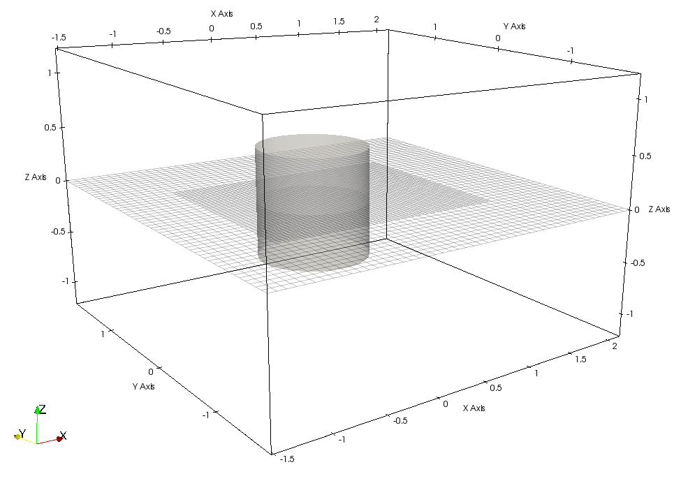
Both the high solidity UNH-RVAT and medium solidity RM2 turbines were modeled using the ALM inside a Reynolds-averaged Navier–Stokes (RANS) simulation, closed with the standard $k$–$\epsilon$ turbulence model. These rotors provide diverse parameters, which helped evaluate the robustness of the ALM. The simulations were performed inside a domain similar in size to that used in Bachant and Wosnik (2016) to approximatel (including blockage) the tow tank experiments (3.66 m wide, 2.44 m tall, 1.52 m upstream and 2.16 m downstream), with similar velocity boundary conditions: 1 m/s inflow, no-slip (fixed to 1 m/s) walls and bottom, and a rigid slip condition for the top, to approximate some effects of the tow tank’s free surface. Simulations were run for a total of 6 seconds, with the latter half used to calculate performance and wake statistics. Pressure–velocity coupling for the momentum equation was achieved using the PISO (pressure implicit splitting of operators) method. A slice of the mesh in the $x$–$y$ plane is shown in Figure 3.

Figure 3: Computational domain used for the RANS ALM simulations. All dimensions are in meters, flow is oriented in the $+x$-direction, and the cylindrical region represents the swept area of the UNH-RVAT rotor. Note that increased mesh refinement was used for the LES simulations.

Similar numerical settings were used for each turbine as well. The Sheng et al. DS model was used with the default coefficients given in Sheng et al. (2008), and the Goude flow curvature correction was employed. A second order backward difference was used for advancing the simulation in time, and second order linear schemes were used for the majority of the terms’ spatial discretizations. The only major difference between the two simulation configurations was that the end effects model was deactivated for the RM2, since it reduced $C_{P}$ far below the experimental measurements. This modification is consistent with the RM2 blades’ higher aspect ratio (15 versus the UNH-RVAT’s 7.1) and tapered planform, though will need to be investigated further. The number of elements per actuator line was set to be approximately equal to the total span divided by the Gaussian force projection width $\epsilon$. Case files for running all the simulations presented here with OpenFOAM v5.0 are available from Bachant (2018a, b).

9.1 Verification

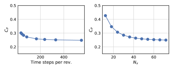
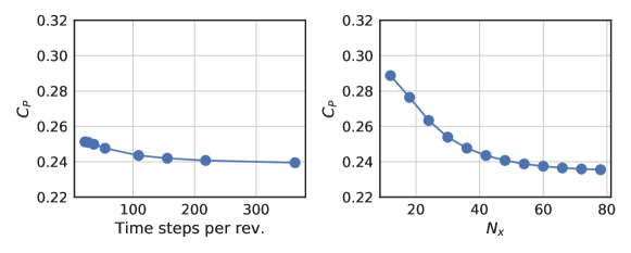
Verification for sensitivity to spatial and temporal grid resolution was performed for both the UNH-RVAT and RM2 RANS cases at their optimal tip speed rations, the results from which are plotted in Figure 4 and Figure 5, respectively. Similar to the verification strategy employed in Bachant and Wosnik (2016), the mesh topology was kept constant, and the resolution was scaled proportional to the number of cells in the $x$-direction $N_{x}$ for the base hexahedral mesh, which was essentially uniform in resolution in all directions. Both models displayed low sensitivity to the number of time steps per revolution. Spatial grid dependence, however, was more important.

Final spatial grid resolutions were chosen as $N_{x}=48$ for both the UNH-RVAT and RM2 cases. Time steps were chosen as $\Delta t_{0}=0.01$ and $\Delta t_{0}=0.005$ seconds for the UNH-RVAT and RM2 respectively, which correspond to approximately 200 steps per revolution. The chosen values should provide $C_{P}$ predictions within one percentage point of the true solution, which is on the order of the expanded uncertainty of the experimental measurements. Note that for computing performance curves, the number of steps per revolution was kept constant, i.e., the time step was adjusted to $\Delta t=\Delta t_{0}\lambda_{0}/\lambda$, where $\lambda_{0}$ was the tip speed ratio roughly corresponding to peak $C_{P}$ as observed in experiments, which was used for verifying the numerical sensitivity to spatial and temporal resolution.

Figure 4: Temporal (left) and spatial (right) grid resolution sensitivity results for the UNH-RVAT ALM RANS model.

Figure 5: Temporal (left) and spatial (right) grid resolution sensitivity results for the RM2 ALM RANS model.

9.2 UNH-RVAT RANS

Power and overall rotor drag (a.k.a. thrust) coefficient curves are plotted for the UNH-RVAT in Figure 6. The ALM was successful at predicting the performance tip speed ratios up to $\lambda_{0}$, which suggests that dynamic stall was being modeled accurately, but $C_{P}$ was overpredicted at high $\lambda$. This may have been caused by the omission of additional parasitic drag sources such as roughness from exposed bolt heads located far enough from the axis to have a large effect at high rotation rates, or an underestimation of the blade–strut connection corner drag coefficient. In Rawlings (2008); Bachant et al. (2016) it was shown how these losses can be significant even with carefully smoothed struts and strut-blade connections. Overprediction of performance at high tip speed ratio could also be a consequence of the Leishman–Beddoes dynamic stall model, which can also be seen in the Darrieus VAWT momentum model results shown in Figure 6.70 of Paraschivoiu (2002).

Figure 6: Power and drag coefficient curves computed for the UNH-RVAT using the actuator line model with RANS, compared with experimental results from Bachant and Wosnik (2016).

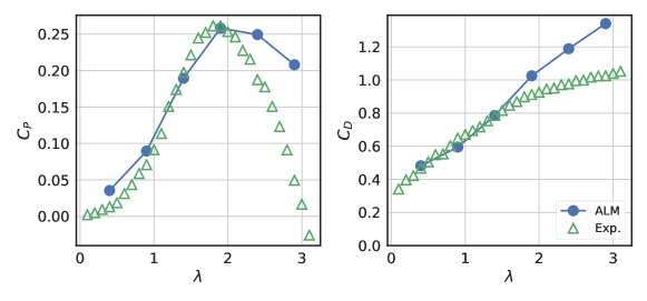
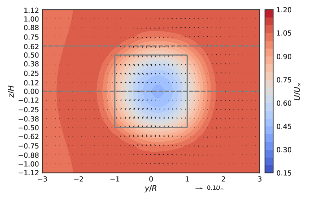
Figure 7 shows mean velocity field for the UNH-RVAT computed by the ALM RANS model. The asymmetry observed in the experiments Bachant and Wosnik (2015) was captured well, along with some of the vertical flow due to blade tip vortex shedding, though the flow structure is missing the detail present in the experiments and blade-resolved RANS simulations. Overall, the wake appears to be over-diffused, which could be a consequence of the relatively coarse mesh. Note that with the DS and flow curvature corrections turned off, the direction of the mean swirling motion reverses, which highlights the importance of resolving the correct azimuthal location of blade loading.

Figure 7: UNH-RVAT mean velocity field at $x/D=1$ computed with the ALM coupled with a $k$–$\epsilon$ RANS model.

Turbulence kinetic energy contours (including resolved and modeled energy) are shown in Figure 8. The ALM was able to resolve the concentrated area of $k$ on the $+y$ side of the turbine, present in the experiments Bachant and Wosnik (2015), but the turbulence generated by the dynamic stall vortex shedding process is absent. This makes sense since in the ALM, the DS model only modulates the body force term in the momentum equation, which does not provide a mechanism for mimicking shed vortices or turbulence.

Figure 8: UNH-RVAT turbulence kinetic energy contours at $x/D=1$ predicted by the ALM inside a $k$–$\epsilon$ RANS model.

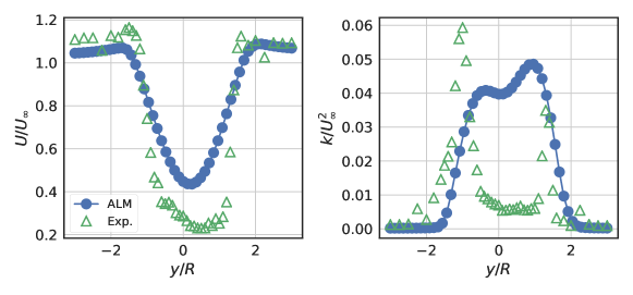
Profiles of mean streamwise velocity and turbulence kinetic energy are shown in Figure 9. Here the over-diffused or over-recovered characteristic of the mean velocity deficit seen in Figure 7 is more apparent. This effect is also seen in the profile of $k$, where energy is smeared over the center region of the rotor.

Figure 9: Mean streamwise velocity (left) and turbulence kinetic energy (right) profiles at $z/H=0$ for the UNH-RVAT ALM, compared with the experimental data from Bachant and Wosnik (2016).

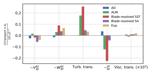
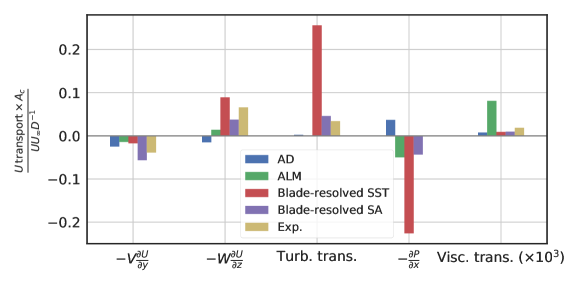
Weighted averages for the terms in the streamwise momentum equation were computed identically as they were in Bachant and Wosnik (2015, 2016), and are plotted in Figure 10 along with the actuator disk (AD) results from Bachant and Wosnik (2015), 3-D blade-resolved RANS results from Bachant and Wosnik (2016) and experiments. The most glaring discrepancy is the ALM’s prediction of positive cross-stream advection, which is caused by the lack of detail in the tip vortex shedding. The total for vertical advection, however, is close to that predicted by the 3-D blade-resolved Spalart–Allmaras model. Levels of turbulent transport due to eddy viscosity and deceleration due to the adverse pressure gradient are between those predicted by the 3-D blade-resolved $k$–$\omega$ SST and SA models. Overall, however, one might expect the total wake recovery rate to be comparable between all models except the actuator disk, which induces negative vertical advection, very little turbulent transport, and has a positive pressure gradient contribution. These results suggests the ALM would be an effective tool—much better than an actuator disk—for assessing downstream spacing of subsequent CFTs, though blade–vortex interaction for very tightly spaced rotors may not be captured, at least on relatively coarse meshes as used here.

Figure 10: Weighted average momentum recovery terms for the actuator disk (AD) simulation from Bachant and Wosnik (2015), UNH-RVAT actuator line model with a $k$–$\epsilon$ RANS closure, the two 3-D blade resolved RANS models described in Bachant and Wosnik (2016) ($k$–$\omega$ SST and Spalart–Allmaras, SA), and the experiments reported in Bachant and Wosnik (2015).

9.3 RM2 RANS

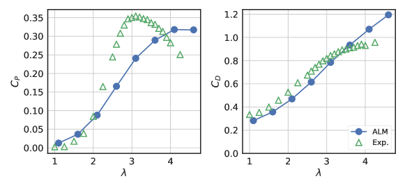
Figure 11 shows the performance curves computed for the RM2 by the ALM, and those from the tow tank experiments Bachant et al. (2016). As with the high solidity RVAT, $C_{P}$ is overpredicted at high $\lambda$. However, $\lambda_{0}$, the tip speed ratio of peak power coefficient, is also shifted to the right. This is indicative of inaccurate dynamic stall modeling, which could possibly be attributed to one of the models’ tuning constants, e.g., the time constant $T_{\alpha}$ for the lagged angle of attack. Limited ad hoc testing revealed that the mean $C_{P}$ at $\lambda_{0}$ more closely matched experimental measurements with $T_{\alpha}$ roughly double the default value given in Sheng et al. (2008). This could be investigated further by looking at the phase of, e.g., maximum $C_{P}$ peaks compared to the experimental values (or possibly those from blade-resolved CFD), but for the present study only mean values were considered.

Figure 11: Power and drag coefficient curves computed for the RM2 using the ALM, compared with experimental data from Bachant et al. (2016).

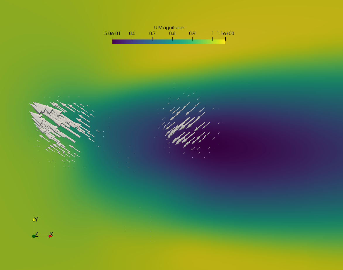
The internal rotor flow about the horizontal center plane, along with the directions and relative magnitudes of the actuator line force vectors are shown in Figure 12. It can be seen how flow features like dynamic stall vortices are not captured with the ALM, despite forces themselves being modulated by the dynamic stall model. This combined with the diffusive nature of the RANS model helps explain discrepancies in predicted power coefficient. With the computational affordability of the ALM coupled with RANS comes a compromise in flow detail, which should be acceptable for array-level simulation, but for individual device design a blade-resolved simulation would be more advisable.

Figure 12: Velocity magnitude and actuator line force field vectors for the RM2 RANS simulation at 6 seconds simulated time.

The mean near-wake structure for the RM2 looked qualitatively similar to the RVAT ALM RANS case, but for the RM2, the effects of blade tip vortex shedding were weaker, which is consistent with experiments Bachant et al. (2016). Nonetheless, the mean vertical flow towards the $x$–$y$ center plane was captured, which is an important qualitative feature of both CFT near-wakes. Like for the UNH-RVAT, predicted turbulence kinetic energy values were concentrated on the $+y$ side of the rotor. However, overall levels of turbulence are lower than for the UNH-RVAT, which is also consistent with the experimental results.

As for the UNH-RVAT RANS case, a mean streamwise momentum transport analysis was undertaken for the RM2 near-wake by computing weighted sums of each term across the entire domain in the $y$–$z$ directions. Similar results as for the UNH-RVAT were obtained, i.e., cross-stream advection was predicted to be positive where it should have been negative, vertical advection was predicted reasonably well, and turbulent transport due to the eddy viscosity was also relatively large. The ratio of wake transport compared with the UNH-RVAT RANS case (approximately 60% to 70% lower for the RM2) matches well with that computed from the experiments, which shows the ALM may successfully predict larger optimal array spacing for the RM2 versus UNH-RVAT.

9.4 UNH-RVAT LES

The state-of-the-art in high fidelity turbine array modeling uses the actuator line method coupled with large eddy simulation (LES), which allows more of the turbulent energy spectrum to be directly resolved, only requiring the dynamics of the smallest scales—where dissipation occurs—to be computed by the so-called subgrid-scale (SGS) model. Since the ALM LES approach has only been reported in the literature for a very low Reynolds number 2-D CFT Shamsoddin and Porté-Agel (2014), and CFTs may provide unique opportunities to array optimization, which could be explored with LES, it was of interest to determine how well the ALM coupled with LES might predict wake dynamics of a higher $Re$ 3-D CFT rotor.

Thus, the UNH-RVAT baseline case was simulated using the Smagorinsky LES turbulence model Smagorinsky (1963), which was the first of its kind, and serves as a good baseline for LES modeling since its behavior is well-reported in the literature, especially for ALM simulations. OpenFOAM’s default Smagorinsky model coefficients were used (giving an approximate equivalent Smagorinsky coefficient $C_{S}=0.17$), and the LES filter width was set as the cube root of the local cell volume. The tip speed ratio was set to oscillate sinusoidally about $\lambda_{0}$ with a 0.19 magnitude and the angle of the first peak at 1.4 radians—similar to the rotation presribed in the blade-resolved RANS simulations discussed in Bachant and Wosnik (2016).

Since the computational cost of LES is significantly higher than RANS, verification with respect to grid dependence was not performed. Instead, mesh resolution was chosen relative to similar studies of turbine wake ALM LES. Of the studies surveyed Shamsoddin and Porté-Agel (2014); Archer et al. (2013); Martínez-Tossas et al. (2015); Troldborg et al. (2007), the mesh resolution ranged from 18–64 points per turbine diameter. The mesh here was set accordingly by using a 16 point per meter base mesh, and refining twice in a region containing the turbine to produce a 64 point per turbine diameter/height resolution. The solver was run with a 0.002 second time step, which is significantly within the limit described by Martínez-Tossas et al. (2015), where an actuator line element may not pass through more than one cell per time step. With these resolutions computation times were $O(10)$ CPU hours per second of simulated time (on 4 processors), which was approximately two orders of magnitude lower than for blade-resolved RANS.

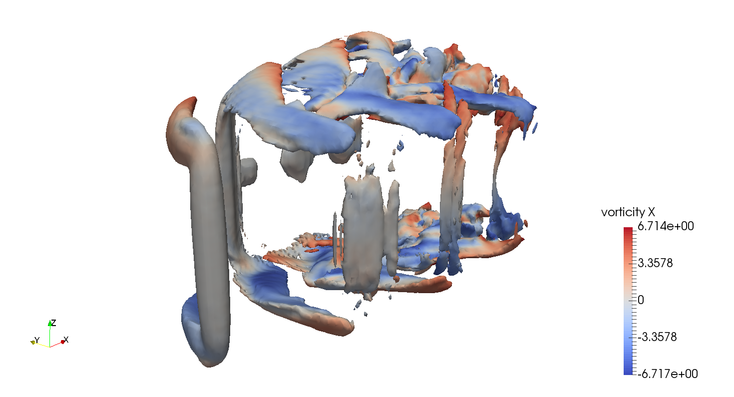
Mean power coefficient predictions for the UNH-RVAT at its optimal mean tip speed ratio dropped to 0.20 using the ALM within the large eddy simulation. However, the amount of information regarding the wake dynamics was greatly increased, even beyond that of the 3-D blade-resolved RANS. Figure 13 shows an instantaneous snapshot of isosurfaces of vorticity produced by the actuator lines.

Figure 13: Snapshot of vorticity isosurfaces (colored by their streamwise component) at $t=6$ s for the UNH-RVAT LES case.

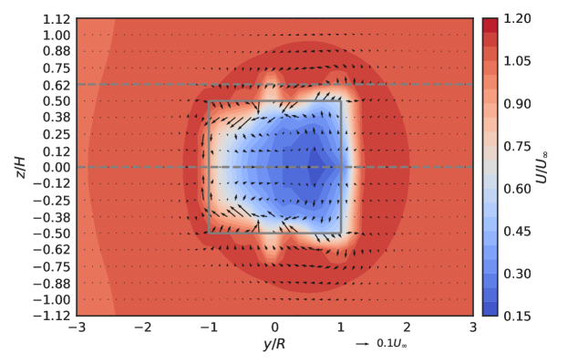
The near-wake’s mean velocity field at $x/D=1$ is shown in Figure 14. Compared with the RANS ALM results, the LES looks much more like the blade-resolved and experimental results Bachant and Wosnik (2015), showing the clockwise and counterclockwise mean swirling motion on the $-y$ and $+y$ sides of the rotor, respectively.

Figure 14: Mean velocity field in the UNH-RVAT near-wake at $x/D=1$ computed with the Smagorinsky LES model.

Contours of turbulence kinetic energy sampled at $x/D=1$ from the large eddy simulation are plotted in Figure 15. Compared with RANS, LES is more able to predict the turbulence generated by the blade tip vortex shedding and dynamic stall effects, though the total turbulence kinetic energy was lower, especially on the $+y$ side of the rotor. This is likely a consequence of the SGS modeling, where the vortical structures generated by the blades remain stable further downstream. Similar effects were seen in Martínez-Tossas et al. (2015); Shamsoddin and Porté-Agel (2014), where higher levels of the Smagorinsky coefficient delayed vortex breakdown and subsequent higher levels of turbulence. Figure 13 shows evidence of these effects, where the blade bound and tip vortices are still relatively coherent at $x/D=1$.

Figure 15: Turbulence kinetic energy in the UNH-RVAT near-wake at $x/D=1$ computed with the Smagorinsky LES model.

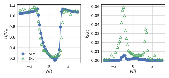
Mean velocity profiles at the turbine center plane, plotted in Figure 16, were predicted more accurately using LES versus RANS, and rival those of the 3-D blade-resolved models. However, turbulence kinetic energy profiles did not match as closely with experiments. Though the qualitative shape was resolved better than that by the RANS ALM simulation, notably the asymmetric peaks around $y/R=\pm 1$, the turbulence generated in the large eddy simulation was approximately an order of magnitude too low. Note that $k$ (both resolved and SGS) does increase significantly downstream after the transition in grid resolution, which implies the grid can help compensate for the artificial stability of the vortex structures caused by the Smagorinsky model. It is hypothesized that the turbulence kinetic energy would better match experimental data taken further downstream, meaning the model should perform well for array simulations with spacing as close as $2D$.

Figure 16: Mean velocity profiles in the UNH-RVAT near-wake at $x/D=1$ and $z/H=0$ computed with the Smagorinsky LES model, compared with experimental data from Bachant and Wosnik (2016).

The planar weighted sums of streamwise momentum recovery terms were computed in the same way as for the RANS cases with the exception of the turbulent transport term, which for the LES was computed from the $x$-components of the divergence of the resolved and SGS Reynolds stress tensors:

$$\text{Turb. trans.}=-\left(\frac{\partial}{\partial x_{j}}\overline{u^{\prime}_{x}u^{\prime}_{j}}+\frac{\partial}{\partial x_{j}}R_{xj}\right),$$ (21)

where $u$ indicates the resolved or filtered velocity, and $R$ is the subgrid-scale Reynolds stress.

Transport term weighted sums computed from the LES results are shown in Figure 17. Unlike the RANS ALM cases, the cross-stream advection contributions are negative, as they are in the experiment and blade-resolved CFD models. The vertical advection term is positive as expected, though smaller than in other cases. Interestingly, the turbulent transport is negative in the LES, meaning the combined effects of the resolved and SGS stressed are transferring momentum out of the wake. The low turbulent transport appears to be partially balanced by higher levels of viscous diffusion—about an order of magnitude larger than the 3-D blade-resolved RANS models and experiments. These discrepancies highlight the difficulty of predicting the near-wake dynamics, the importance of the SGS model in LES, and the need for data further downstream to test and refine predictions for wake evolution. For example, setting the Smagorinsky coefficient higher may induce vortex breakdown earlier, which would raise the turbulence levels significantly.

Figure 17: Weighted average momentum recovery terms at $x/D=1$ for the RVAT ALM LES using the Smagorinsky SGS model.

10 Conclusions

An actuator line model for cross-flow turbines, including a Leishman–Beddoes type dynamic stall model, flow curvature, added mass, and lifting-line based end effects corrections, was developed and validated against experimental datasets acquired for high and medium solidity rotors at scales where the performance and near-wake dynamics were essentially Reynolds number independent. When coupled to a $k$–$\epsilon$ RANS solver ALM simulations took $O(0.1)$ CPU hours per second of simulated time, while when coupled with a Smagorinsky LES model the computing time was $O(10)$ hours per second, which represent a four and two order of magnitude decrease in computational expense versus 3-D blade-resolved RANS Bachant and Wosnik (2016), respectively.

The RANS ALM predicted the UNH-RVAT performance well at tip speed ratios up to and including that of max power coefficient. The RM2 power coefficient on the other hand was underpredicted at lower $\lambda$. Both models overestimated $C_{P}$ at the highest tip speed ratios, which has been observed in other simulations using Leishman–Beddoes type dynamic stall models. Possible explanations include underestimation of added mass effects or blade–strut connection corner drag, incorrect time constants in the LB DS model, and/or inaccuracy due to the virtual camber effect. In the present flow curvature model, the angle of attack is corrected, but the foil coefficient data is not transformed, meaning the LB DS separation point curve fit parameters are equal for both positive and negative angles of attack. A foil data transformation algorithm based on virtual camber should be investigated for future improvement of the ALM.

The RANS ALM cases were able to match some important qualitative near-wake flow features, e.g., the mean vertical advection velocity towards the mid-rotor plane. However, the mean flow structure and turbulence generation due to blade tip and dynamic stall vortex shedding shows some discrepancy with experimental and blade-resolved CFD. Extensions to the ALM to deal with these shortcomings should be developed, e.g., a turbulence injection model as employed by James et al. James et al. (2010) or a model that will “turn” the ALM body force vectors to approach the effects of leading and trailing edge vortex shedding during dynamic stall.

The UNH-RVAT was simulated with the ALM embedded within a typical Smagorinsky LES, which thanks to its lower diffusion and/or dissipation was able to more accurately capture the large scale vortical flow structures shed by the rotor blades. Turbulence generated by the blade tip vortex shedding and dynamic stall region of the blade path was better resolved, but overall lower levels of turbulence were predicted, which is likely a consequence of the subgrid-scale model’s influence on the stability of shed vortices. This effect was also apparent in the negative predictions of turbulent transport on the streamwise momentum recovery. Therefore, subgrid-scale modeling should be investigated further before applying the ALM LES to array analyses.

The ALM provides a more physical flow description compared to momentum and potential flow vortex models, at a reasonable cost. The ALM also drastically reduces computational effort compared to blade-resolved CFD, while maintaining the unsteadiness of the wake not resolved by a conventional actuator disk. When combined with RANS the ALM will allow VAT array simulations on individual PCs, and with high performance computing and LES the ALM is one of the highest fidelity array modeling tools available. Ultimately, the ALM will help reduce dependence on expensive physical modeling to optimize VAT array layouts.