Stony Brook University, Stony Brook, NY 11794, USA Department of Physics, Technion, Haifa 32000, Israel
The holographic dual of a Riemann problem in a large number of dimensions
Abstract
We study properties of a non equilibrium steady state generated when two heat baths are initially in contact with one another. The dynamics of the system we study are governed by holographic duality in a large number of dimensions. We discuss the “phase diagram” associated with the steady state, the dual, dynamical, black hole description of this problem, and its relation to the fluid/gravity correspondence.
1 Introduction
The Riemann problem may provide a relatively simple setting in which to study the non-equilibrium physics of quantum field theory. The problem asks for the time evolution of piece wise constant initial conditions with a single discontinuity in the presence of some number of conservation laws, for example of energy, momentum, mass, or charge. In our case, we consider a fluid phase of a conformal field theory (CFT) with an initial planar interface, where the energy density jumps from on the left of the interface to on its right. We also allow for a discontinuity in the center of mass velocity of the fluid across the interface.
For simplicity, we will make a number of further restrictions. We assume a conformal field theory that has a dual gravity description via the AdS/CFT correspondence. A priori, this will allow us to study the system beyond the hydrodynamic limit. We also take the limit that the number of spatial dimensions is very large. In this limit, we find that the system is described by two conservation equations
| (1) |
where is, up to gradient corrections, the energy density and the energy current. These equations are a special case of equations derived in ref. Emparan:2015gva . In these variables the Riemann problem amounts to a determination of and given an initial configuration of the form
| (2) |
By choosing an appropriate reference frame, we may set without loss of generality.
As it happens, there are extensive treatments of this type of Riemann problem in hydrodynamics textbooks. See for example ref. Smoller . Typically, a pair of rarefaction and/or shock waves form and move away from each other, creating in their wake a region with almost constant and . In recent literature, this intermediate region has been called a non-equilibrium steady state (NESS) Bernard:2012je ; Bernard:2016nci . One of the main results of this paper is a “phase” diagram valid in a large limit (see figure 1) that describes, given the conservation equations (1) and initial conditions (2), which pair of waves are formed: rarefaction-shock (RS), shock-shock (SS), shock-rarefaction (SR), or rarefaction-rarefaction (RR).

A physical reason for the preference of a rarefaction wave to a shock wave is entropy production.
Recent interest in this type of Riemann problem was spurred by a study of the problem in dimensional conformal field theory Bernard:2012je where the evolution is completely determined by the conformal symmetry and a hydrodynamic limit need not be taken. Conservation and tracelessness of the stress tensor imply that the stress tensor is a sum of right moving and left moving parts. When one finds a NESS in between the two asymptotic regions, characterized by an energy density and an energy current proportional to . The NESS is separated from the asymptotic regions by outward moving shock waves traveling at the speed of light. (An extension of the analysis of Bernard:2012je which includes a discontinuity in the center of mass velocity, holomorphic currents and chiral anomalies can be found in Chang:2013gba . An analysis of shock waves and their relation to two dimensional turbulence was carried out in Liu:2010jg .)
In more than two space-time dimensions, conformal symmetry alone is not enough to specify the evolution completely and one needs additional assumptions about the structure of the conserved currents. Recent work appealed to the gauge/gravity duality Bhaseen:2013ypa ; Amado:2015uza ; Megias:2015tva ; Bakas:2015hdc , an analogy with dimensions Chang:2013gba , and hydrodynamics Bhaseen:2013ypa ; Pourhasan:2015bsa ; Lucas:2015hnv ; Spillane:2015daa . These papers focused on the case and such that from a hydrodynamic perspective a left moving rarefaction wave and a right moving shock wave are expected to emerge.
The distinction between rarefaction and shock waves was ignored in some of these papers Bhaseen:2013ypa ; Chang:2013gba ; Pourhasan:2015bsa . Indeed, when working with or dimensional conformal field theories, the difference between, say, an SS solution to the Riemann problem and an RS solution to the Riemann problem is very small for all but extreme initial energy differences. As the spacetime dimension increases however, the difference between a rarefaction wave type of solution and a shock wave solution becomes significant Spillane:2015daa . This amplification of the difference between the two solutions serves as a motivator for studying this Riemann problem in a large number of dimensions.
Interestingly, a large limit has independently been a topic of recent interest Emparan:2015gva ; Emparan:2016sjk ; Bhattacharyya:2015dva ; Bhattacharyya:2015fdk ; Emparan:2013moa ; Emparan:2013xia ; Emparan:2013oza ; Emparan:2014cia ; Emparan:2014jca ; Emparan:2014aba ; Emparan:2015rva ; Andrade:2015hpa ; Romero-Bermudez:2015bma in the study of black hole solutions to Einstein’s equations. Of particular relevance to our work is the connection between black holes in asymptotically AdS spaces and hydrodynamics Bhattacharyya:2008jc . Certain strongly interacting conformal field theories are known to have dual classical gravitational descriptions. In the limit where these conformal field theories admit a hydrodynamic description, a solution to the relevant hydrodynamic equations can be mapped to a solution of Einstein’s equations, in a gradient expansion where physical quantities change slowly in space and time. Transport coefficients such as shear viscosity are fixed by the form of Einstein’s equations. Thus, one may study the Riemann problem in conformal field theories with a large number of dimensions by studying an equivalent Riemann-like problem involving an initially discontinuous metric of a black hole in an asymptotically AdS background.
Given that extensive analyses of conservation equations like (1) can be found in many hydrodynamics textbooks and papers, one can legitimately ask why we bother to redo the analysis here. The reason is that when working in a large number of dimensions, one can solve for the black hole metric exactly, independent of the derivative expansion (which is naturally truncated), thus obtaining an exact solution to the Riemann problem which includes possible viscous terms and is in general valid even when gradients of thermodynamic quantities are large (as is the case with discontinuous initial conditions).
Our work is organized as follows. In section 2, we rederive the equations (1) by taking a large limit of Einstein’s equations. We show how to rewrite them as the conservation condition on a stress-tensor, . In section 3, we compare the large stress tensor and equations of motion to those arising from the fluid-gravity correspondence Bhattacharyya:2008jc . We find that both eqs. (1) and the stress tensor are equivalent to the hydrodynamic equations that come from the fluid-gravity correspondence at large , at least up to and including second order gradient corrections. In the same section we also construct an entropy current using an area element of the black hole horizon and show that the divergence of the entropy current is positive in this large limit. In section 4, we solve the Riemann problem for eqs. (1) and derive the phase diagram given in figure 1. Finally, we conclude in section 5 with some directions for future research. Appendix A contains a short calculation of the entropy produced across a shock, while appendix B contains plots of auxiliary numerical results.
2 The holographic dual of the Riemann problem for large
We wish to construct a holographic dual of the Riemann problem. Consider the Einstein Hilbert action
| (3) |
A canonical stationary solution of the resulting equations of motion is the black brane solution
| (4) |
where is an integration constant which denotes the Hawking temperature. The solution (4) is dual to a thermal state of a conformal field theory with temperature . For instance, the thermal expectation value of the stress tensor in such a state is given by
| (5) |
where
| (6) |
is the pressure with a theory dependent dimensionless parameter. (The indices and run over the dimensions of the -dimensional CFT.)
As discussed in Amado:2015uza a dual description of the Riemann problem necessitates an initial black hole configuration which is held at some fixed temperature for all and at a different temperature for . This would correspond to a configuration where the expectation value of the stress tensor is given by (5) with for and by (5) with for . Since the initial black hole is out of equilibrium it will evolve in time. Its dual description will provide a solution for the time evolution of the stress tensor which we are after. Thus, our goal is to solve the equations of motion following from (3) and use them to construct the dual stress tensor.
An ansatz for the metric which is compatible with the symmetries and our initial conditions is given by
| (7) |
where the metric components are functions only of , , and . (A more general ansatz which involves a transverse velocity can be found in Emparan:2015gva .) A numerical solution of the equations of motion for , and ( or ) with smoothened initial conditions has been obtained for in Amado:2015uza for relatively small initial temperature differences, . A solution for finite and for large temperature differences, is challenging.
In this work we use the methods developed in Emparan:2015gva ; Emparan:2016sjk (see also Bhattacharyya:2015dva ; Bhattacharyya:2015fdk ; Emparan:2013moa ; Emparan:2013xia ; Emparan:2013oza ; Emparan:2014cia ; Emparan:2014jca ; Emparan:2014aba ; Emparan:2015rva ) to address the Riemann problem in the limit that is very large. Such a limit can be understood as follows. In an appropriate gauge, the near boundary expansion of the metric gives
| (8) | ||||
Thus, in the large limit at any finite value of , the spacetime looks like the AdS vacuum. Only by keeping finite with will the corrections to the metric remain observable. Our strategy is to solve the equations of motion in the finite region subject to the boundary conditions (8). Following Emparan:2015gva , we also use the scaling and so that in this coordinate system the line element takes the form
| (9) |
where
| (10) | ||||
(In a slight abuse of notation is now either or .) We have used the letters and to emphasize these quantities’ (soon to be seen) close connection with an energy density and energy current in the dual hydrodynamic description.
One can now solve the equations of motion order by order in . The equations of motion are simply Einstein’s equations in the presence of a negative cosmological constant:
| (11) |
setting for convenience. Let and index the , , and directions only, while and index the remaining perpendicular directions. Furthermore, let be the Ricci tensor with respect to the three dimensional metric in the , , and directions. Then
| (12) | |||||
| (13) |
Imposing that the boundary metric is Minkowski and choosing a near boundary expansion of the form (8) we find
| (14) | ||||
where the correction to and the contributions to are too long to write explicitly. The functions and are functions of and only and must satisfy the additional constraints (1). Equations (1) are identical to those obtained in Emparan:2015gva ; Emparan:2016sjk . We can rewrite them in terms of a conservation law
| (15) |
where
| (16) |
where is an arbitrary function. Likewise, the functions and must also satisfy a set of equations which can be obtained from the conservation of
| (17) |
where
| (18) |
We will use ′ and interchangeably in what follows.
3 Comparison with hydrodynamics
Let us pause to understand (16). Within the context of the gauge-gravity duality it is possible to construct a solution to the Einstein equations which is perturbative in , and derivatives of the metric components Bhattacharyya:2008jc . Such a perturbative solution to the equations of motion, which is available for any dimension Haack:2008cp ; Bhattacharyya:2008mz , allows for a dual description of the theory in terms of fluid dynamical degrees of freedom.
3.1 Stress tensor from fluid-gravity correspondence
To construct the dual hydrodynamic description of a slowly varying black hole, we boost the black hole solution (4) by a constant velocity in the , , directions. The resulting line element is given by
| (19) |
Allowing for and to become spacetime dependent implies that (19) will get corrected. By setting gradients of and to to be small, one can solve for the corrections to (19) order by order in derivatives so that the line element will take the schematic form
| (20) |
where denotes the th order gradient corrections to the line element.
The stress tensor which is dual to (19) takes the form
| (21) |
also expanded in gradients. One finds Haack:2008cp ; Bhattacharyya:2008mz
| (22) |
which is nothing but a boosted version of (5) and then, in the Landau frame,
| (23) | ||||
with
| (24) | ||||
and
| (25) |
(Note that our definition of is somewhat unconventional.) An initial analysis of third order gradient corrections has been carried out in Grozdanov:2015kqa for . A full analysis of all third order transport terms for arbitrary dimension is currently unavailable.
Since (16) has been obtained from a large limit of a gravitational dual theory, we expect that (16) coincides with (21) when the former is expanded in derivatives and the latter is expanded around large . In short, we expect that taking a gradient expansion commutes with taking a large limit. To make a direct comparison let us consider the hydrodynamic stress tensor (21) in the , , coordinate system where the metric tensor takes the form
| (26) |
One important effect of this rescaling is to keep the sound speed to be an order one quantity.
Scaling the spatial component of the velocity field by , viz.,
| (27) |
and maintaining that is finite in the large limit, we find,
| (28) | ||||
and thus,
| (29) |
where
| (30) |
and denotes third order and higher derivative corrections. Note that this constitutive relation for the stress tensor includes and encodes the large limit of the transport coefficients (25).
Now, we insert the redefinitions
| (31) | ||||
into the large constitutive relation for the stress tensor (16), use the large stress tensor conservation equations (1), and throw out terms that have three or more derivatives. We claim that in this fashion, we recover the stress tensor (29) in the gradient expansion. Thus, the large limit and the gradient expansion seem to commute. Note that while the conservation equations (1) are of second order in gradients of and , the stress tensor includes at least second order gradients.
The implications of (31) are worth emphasizing. The equations of motion (1) are equivalent to the standard equations of motion of relativistic hydrodynamics when the latter are expanded in a large limit. When working with the and variables one obtains equations of motion which are second order in derivatives and therefore include dissipative effects. When carrying out a frame transformation to the more traditional Landau frame, more derivatives will appear. When considering the stress tensor associated with the equations of motion (1) one obtains more terms with higher gradients which do not contribute to the equations of motion. It would be interesting to see if one can construct an alternative to the Israel-Stewart theory using a “large -frame” where gradients naturally truncate.
3.2 Entropy from Gravity
Within the context of our forthcoming analysis, it is instructive to compute the dual entropy production rate which is associated with the evolution of the horizon. Due to its teleological nature, it is usually difficult to identify the location of the event horizon. However, in the large limit the analysis is somewhat simplified. Let us look for a null surface of the form . The normal to such a surface is
| (32) |
Demanding that implies, to leading order in the large limit, that
| (33) |
The spacetime singularity which exists in our solution implies that an event horizon must be present. Since the only null surface available is (33), it must be the location of the event horizon. Subleading corrections to the location of the event horizon are given by
| (34) | ||||
To compute the change in the black hole entropy over time we compute the area form of the event horizon. Following the prescription of Bhattacharyya:2008xc , we find that
| (35) |
where
| (36) |
where is the spatial part of the induced metric on the horizon
| (37) |
and is defined via
| (38) |
A short computation yields
| (39) | ||||
Thus,
| (40) |
where we have normalized the entropy density so that it is compatible with our conventions for the energy density.
The second law of black hole thermodynamics amounts to
| (41) |
In our large limit we find that
| (42) |
The expectation from hydrodynamics, to second order in derivatives, is that the divergence of the entropy current is given by
| (43) |
(See for example (8) of ref. Son:2009tf .) This expectation matches (42) on the nose. Note that to leading order in the large limit the entropy current vanishes. This somewhat surprising feature of the large limit follows from the fact that entropy production terms are suppressed by inverse powers of the dimension in the large limit. Another way of understanding this suppression comes from thinking about the temperature . In the large limit, is constant to leading order in . From the thermodynamic relation , it then follows that changes in energy are proportional to changes in entropy, and entropy conservation follows from energy conservation at leading order in a large expansion.111We thank R. Emparan for a discussion on this point.
4 Near equilibrium steady states
We now analyze the dynamics controlled by the partial differential equations (1) which encode the dynamics of an out of equilibrium black hole (7) and its dual stress tensor (16). Various related holographic analyses can be found in Chesler:2009cy ; Chesler:2010bi ; Chesler:2013lia ; Balasubramanian:2013yqa ; Chesler:2015fpa ; Khlebnikov:2010yt ; Shuryak:2012sf ; Fischetti:2012vt ; Figueras:2012rb ; Emparan:2013fha . As discussed in the introduction, the particular question we would like to address is a Riemann problem: What is the time evolution following from an initial condition (2)? We are particularly interested in the steady state solution which will emerge at late times. For convenience we will consider a reference frame for which . Indeed, if and satisfy the conservation equations (1), then so do and . Thus, for constant values of and , we can choose a such that will be set to zero. The non-relativistic nature of the boost symmetry reflects the fact that the large limit we have taken is effectively a non-relativistic limit where the speed of light has been pushed off to infinity.
4.1 Rarefaction waves vs. shock waves
Before addressing the Riemann problem in its entirety let us consider a simplified system which is less constrained. Consider (16) with gradient terms neglected. The resulting expression is the large limit of the energy momentum tensor of an inviscid fluid which is known to support (discontinuous) shock waves Smoller for any finite value of . While the solution to the full Riemann problem will consist of a pair of shock and/or rarefaction waves, we begin in this section with a single discontinuous shock wave moving with velocity . Conservation of energy and momentum imply
| (44) |
where and specify the value of to the left or right of the shock respectively.222In this section we use subscripts and to denote values of quantities to the right or left of the shock. In other sections we use subscripts and to denote quantities in the right and left asymptotic regions. In the latter case there is generally an interpolating region which we denote with a subscript. The conservation conditions (44) are very general and are often referred to as the Rankine-Hugoniot (RH) relations. In our setup they reduce to
| (45) | ||||
where and are the energy density and current immediately to the right or left of the shock. While these Rankine-Hugoniot relations hold for an arbitrary, piece-wise continuous fluid profile, in what follows, we are interested in the much simpler situation where and are constant functions away from the shocks. Amusingly, satisfies a cubic equation,333In general , one finds the relation where is the fluid velocity.
| (46) |
a plot of which as a function of resembles a fish: fixing , each value of is mapped to a point on the plane. The collection of such points is given by a fish-like curve, an example of which is given in the left panel of figure 2.
We make two observations about the fish. The vacuum always lies on the cubic (46), corresponding to the fact that a shock can interpolate between any value of and the vacuum. Also is the point of self-intersection of the cubic and has . The physical content of this observation is that when is close to but still lies on the cubic, we can find a close approximation to the fluid profile by linearizing the equations of motion. As we will describe in greater detail below, linearized fluctuations correspond to damped sound modes, and indeed the two regions can be connected by sound waves propagating at the local sound speed .
The shock solutions we found all solve the conservation equations (45). However, some of these solutions are unphysical in the following sense. Let us boost to a frame where the shock speed vanishes, . In half of the shock solutions, a quickly moving fluid at low temperature is moving into a more slowly moving fluid at higher temperature, converting kinetic energy into heat and producing entropy. We will refer to these shocks as “good” shocks. The other half of the solutions correspond to the time reversed process where a slowly moving fluid at high temperature moves into a rapidly moving but cooler fluid, turning heat into kinetic energy. This second solution, as we shall see shortly, should be discarded.
Strictly speaking, entropy is conserved in the large limit (see the discussion following equation (43)). A more formal way of understanding why one should discard the bad shocks is to restore the gradient corrections but take a limit where these are small. Let us assume that in the frame where the shock velocity is zero there is an approximately stationary configuration such that time derivatives are much smaller than spatial derivatives. Boosting back to a shock with velocity , we expect that and depend only on the combination , i.e., and likewise, . The equations of motion (1) become ordinary differential equations which can be integrated once to obtain
| (47) | ||||
We have picked the two integration constants such that and vanish in the left asymptotic region. The Rankine-Hugoniot conditions (45) imply that and also vanish in the right asymptotic region. As and themselves vanish in the left and right asymptotic regions, we can describe and well near these points by looking at a gradient expansion. Near the left asymptotic region
| (48) | ||||
There is a similar looking equation for and near the right asymptotic region
| (49) |
The solutions near and near have an exponential nature with the sign of the exponents depending on the eigenvalues of and appearing on the right hand side of (48) and (49) given by
| (50) |
We now observe that the signs of the eigenvalues of and determine whether the shock is a viable solution to the equations of motion.
-
•
If both eigenvalues of are negative, then and will not vanish as . Thus we require that at least one eigenvalue of is positive in order for a shock solution to exist.
-
•
If we assume there is exactly one positive eigenvalue, then and . Note that the value corresponds to the slope of one of the characteristics (i.e. the local speed of one of the sound waves), and this condition implies that this characteristic will end on the shock. Since is assumed to be negative, we have to tune one of the two integration constants of the system of differential equations to zero. This tuning means that generically the solution to the right of the shock will be a linear combination of both of the solutions near . If both solutions are to be used, then it had better be that both eigenvalues of are negative. (Otherwise, it will not be true that and vanish in the limit .) In particular, the larger of the two eigenvalues must be negative, which implies that . (In terms of characteristics, both will end on the shock.) Thus, we find the constraint
(51a) -
•
If both eigenvalues of are positive, we still need at least one negative eigenvalue of to be able to connect the solutions in the left and right asymptotic regions. Moreover, for to have two negative eigenvalues would be inconsistent with momentum conservation (45). An analysis similar to the previous one yields
(51b)
The constraints (51) choose the good shocks over the bad ones.444In appendix A, we discuss a third RH relation one can write down for the entropy current. If the RH relations for energy and momentum are satisfied, the RH relation for the entropy current will typically be violated due to entropy production associated with viscous effects. In the weak shock limit, we demonstrate that gradient corrections produce the entropy that leads to this violation of the third RH relation. Reversing the sign of the energy difference between the two asymptotic regions in eqs. (78) or (80), it is straighforward to see that a bad shock would lead to a decrease in entropy, at least in the simple case where and .
Since bad shocks are not allowed, one may inquire as to the time evolution of a discontinuity with initial conditions which would have generated a bad shock. As it turns out, bad shocks can be replaced by the more physical rarefaction solutions Smoller . The rarefaction solution assumes that between the asymptotic regions specified by and , there is an interpolating solution where and are functions of . As was the case for the shock wave, given and , there is a one parameter family of allowed values of and . These are given by
| (52) | ||||
The curve traced by also resembles a fish, and for moderate values of the shock parameters and it closely follows the cubic curve corresponding to a shock solution. (See the central panel of figure 2.) The vacuum solution can always be connected to through a rarefaction wave. The self-intersection point has , again corresponding to a sound wave type interpolation between the two regions .
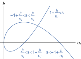
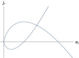
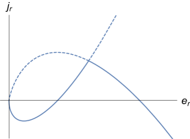
Given that bad shocks are replaced by rarefaction waves, one should remove from the fish diagram (left panel of figure 2) the portion of the curve which corresponds to bad shocks and replace it with a curve corresponding to a rarefaction solution (central panel of figure 2). The resulting curve can be found on the right panel of figure 2: the belly of the fish and the lower part of its tail corresponds to a good shock and its back and upper tail to a rarefaction solution. One may compute the curve explicitly by imposing (51), but it can also be understood from a graphical viewpoint as we now explain.
Recall that the self intersection point of the shock wave fish (solid curve on the left panel of figure 2) corresponds to a shock velocity, , which takes the values of the local speed of sound, . On the tail, is either larger than (upper tail) or smaller than (lower tail). Thus, on the tails, the eigenvalues are either both positive or both negative. The top portion of the tail has while the bottom portion of the tail has . As a result, the top portion of the tail must be replaced by a rarefaction wave while the bottom portion can be a shock. To decide which portion of the body of the shock fish to replace by a rarefaction wave, one must study .
Consider a second fish which exhibits the solution to the cubic (46) for a given value of . We will call this second fish an -fish and the first an -fish. Similar to the analysis of the tail of the -fish, we find that the bottom portion of the tail of the -fish should be constructed from a rarefaction solution while the top portion from a shock.
Consider an -fish whose point of self intersection lies somewhere on the body of the -fish. When the -fish is drawn so that it intersects the back of the -fish, the bottom portion of the -fish’s tail will go through the point of self-intersection of the -fish (see the left panel of figure 3). As the bottom portion of the tail of the -fish is a rarefaction, the region can be connected to by a rarefaction. Reciprocally, since we’re describing a single shock or rarefaction interface between two regions, the back of the -fish should be replaced by a rarefaction wave. We can run the argument again for an -fish drawn to intersect the belly of the -fish. We conclude that the belly of the -fish must be a shock (see the right panel of figure 3).


4.2 Solving the Riemann problem using ideal hydrodynamics
Armed with our understanding of shock waves and rarefaction solutions, let us now tackle the Riemann problem we set out to solve. At , we consider a pair which describes the fluid for and another pair describing the fluid for . For a single interpolating shock or rarefaction, we have seen that given there is a one parameter family of solutions that determine . Thus, generically, there will not be a single shock or rarefaction solution that joins to an arbitrary . However, we can connect the two regions using a pair of shock and/or rarefaction waves. That is, we could connect to an intermediate regime with values of and given by using a shock or rarefaction wave and another shock wave or rarefaction wave to connect the intermediate regime to the right asymptotic region . In all cases, given the initial conditions, the pair of rarefaction and/or shock waves should be such that they move away from each other.
The strategy for determining which type of solution is allowed is to prefer good shocks over rarefaction solutions and rarefaction solutions over bad shocks. Thus, given a pair and we need to establish which of the four possibilities for the time evolution of the initial state is allowed: two shocks (SS), a rarefaction wave followed by a shock (RS), or the remaining two configurations which we will denote by SR and RR.
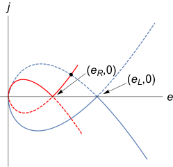
To understand the possible solutions to the Riemann problem, let us first consider two fish diagrams: one associated with (the -fish) and another with (the -fish). The points of overlap of the diagrams will give us the possible value of and . We will always choose a point where the two disturbances are moving away from each other. See, for example, figure 4.
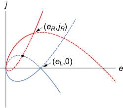
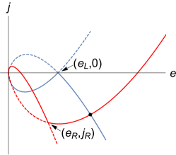
Instead of plotting the - and -fishes, we can obtain closed form expressions for the various types of solutions by solving (51) and (52) on a case by case basis. In the following we provide some simple examples of such expressions.
-
•
RS configurations. As an example of the RS case, we take and as the asymptotic regions with . The SR case is a left-right reflection of the RS case and therefore does not warrant further discussion.
To estimate the values of and we can follow the strategy laid out in Lucas:2015hnv ; Spillane:2015daa . For the left region we use the solution (52) with , , and . For the right region we use (45) with , , and . We find
(53) which, unsurprisingly, coincides with the large limit of the hydrodynamic analysis of Lucas:2015hnv ; Spillane:2015daa .
As pointed out in Lucas:2015hnv the rarefaction solution will cover the location of the original shock discontinuity whenever
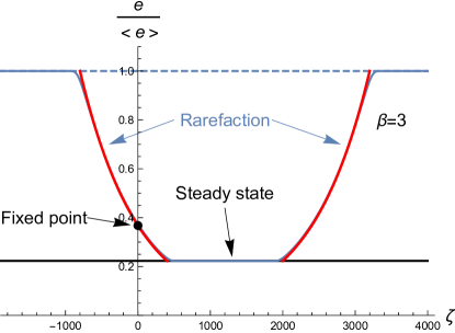
(54) At the point in the rarefaction wave, the values of and are time independent (since any function of will have a fixed point at ). Moreover for a conserved stress tensor , the first spatial derivative of and the first and second spatial derivatives of vanish at this fixed point. Thus, one may think of the pressure at the fixed point as a “short” steady state for long enough times. “Short” implies that the region is of small spatial extent. From this perspective one has split steady states for large enough initial temperature differences. The values of and at the short steady state are given by
(55) -
•
SS configurations. A simple example of the SS case has on the left and on the right with . We compute the NESS by gluing two shock waves to an intermediate region with , similar to the RS case. Setting , the intermediate NESS is given by
(56) and the shock velocities for the left and right moving shocks, and respectively, are given by
(57) (58) -
•
RR configurations. Using and , we can find simple solutions that involve two rarefaction waves.555As it turns out in the RR phase, there is a simple expression for the steady state for all values of , , and , where A fixed point associated with a left moving rarefaction solution occurs whenever and a fixed point associated with the right moving rarefaction solution occurs whenever In this case, the NESS is characterized by
(59) where the left moving rarefaction wave extends from to while the right moving rarefaction wave extends from to with
(60) Similar to the RS case we find that there is a fixed point associated with the left moving wave whenever
(61) with
(62)
We claim that given , the “phase diagram” of figure 1 immediately allows us to choose the correct configuration of shocks and rarefaction waves for any . Indeed, following figure 4, the location of the self intersection point of the -fish will determine the nature of the intersection of the - and -fish: if the intersection point of the -fish lies above the -fish we will always get an RR solution; if the intersection point of the -fish is below the -fish we get an SS solution; and RS and SR solutions will correspond to an intersection point of the -fish in the body or tail of the -fish respectively. Conformal invariance dictates that the phase diagram can depend on the only two dimensionless parameters of this problem, and we obtain the phase diagram in figure 1.
Note that even though the -fish and the -fish intersect at , we can always rule out an intermediate point that corresponds to a vacuum. The vacuum intersection point is always along the bodies of the two fish where we have . As discussed, we can not in general connect the two asymptotic solutions if we do not have two eigenvalues of the same sign (positive for and negative for ) in one of the regions.
4.3 A numerical solution to the Riemann problem.
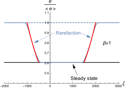
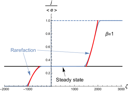
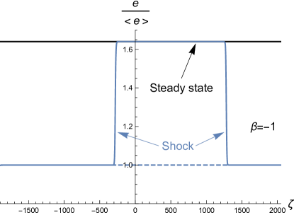
In the previous sections we have obtained predictions for the evolution of and starting from an initial configuration (2) and assuming that gradient corrections to the equations of motion are small. It is somewhat unfortunate that this assumption stands in stark contrast to the discontinuous jump in the initial state and one may inquire whether the analysis of the previous section is relevant for the problem at hand. In order to resolve this issue we solve the full equations of motion (1) numerically. We give numerical examples of the RR, SS, and RS phases described above. To our numerical accuracy, the difference in and between the ideal case which we have studied analytically and the case with gradients included which has been obtained numerically appears to disappear in the long time limit.
As it turns out, the equations (1) are easy to evolve numerically with canned PDE solvers, such as Mathematica’s NDSolve routine Mathematica . To obtain various solutions one can evolve the initial condition
| (63) | ||||
in a periodic box of length . (In appendix B, we use a more elaborate piecewise continuous initial condition.) For sufficiently large, the initial condition approaches a square wave. As long as the disturbance has not travelled a distance of order , causality ensures that the behaviour of and are very close to that of an infinite system where the values of and in the asymptotic region are fixed at some constant value. If we denote these asymptotic values as and then
| (64) |
We can similarly define and .
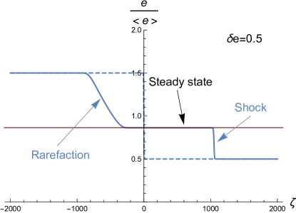
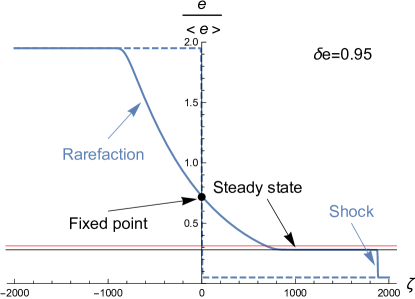
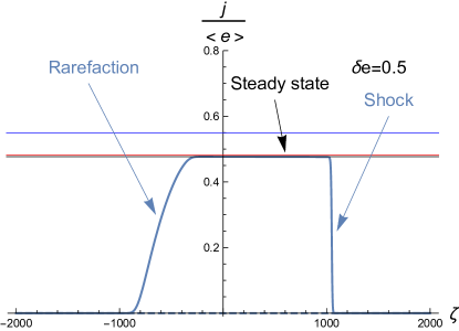
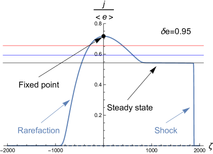
In figures 5, 6, and 7, we have plotted typical results for numerical solutions to (1), corresponding to RS, SS, and RR configurations. The resulting values of and seem to approach the predicted values of and at long times—at least as far as our numerical precision can be trusted (see appendix B). In particular, in the RS case, we approach the steady state value (53); in the SS case, we approach (56); and in the RR case, we approach (59). As we discuss in greater detail in the next section, one place where gradient effects show up and do not disappear as a function of time is in the shock width.


One may speculate that the agreement between the predicted steady state in the absence of gradient corrections and the numerical results is associated to the fact that the gradient corrections, even though order one in our system of units, come with dimensionful coefficients. In the language of the renormalization group, they conform to irrelevant couplings. Perhaps it is for this reason that at long enough time and in a large enough box, we may be able to ignore these corrections for the most part.
4.4 Restoring gradient corrections
In this section, we try to gain a better handle over the gradient corrections and their affect on the predicted steady state values. The analysis here is incomplete and approximate. To overcome the deficiencies of paper and pencil estimates, we include some numerical solutions to the conservation equations (1) that provide support for the estimates. We will consider separately corrections to each of the features we found in the idealized limit: the steady state and asymptotic regions with constant and , a shock wave, a rarefaction wave, and the discontinuity at the edge of the rarefaction.
Corrections to constant regions
Corrections to a constant and region are easiest to analyze. Assuming the fluctuations are small, we look for linearized solutions of the form and . We find two propagating modes
| (65) |
These two modes are damped sound modes whose speed is shifted by the fluid velocity . The gradient corrections appear here in the form of the damping term in the dispersion relation. Given this result, we anticipate that we will be able to correct a constant and region by taking an appropriate linear superposition of sound waves. The damping suggests that at long times the solution can only involve constant and constant .
As a side comment, an odd thing about these mode relations is that they are exact. Recall that in first order viscous hydro, we would typically solve an equation of the form for , in the case of vanishing background fluid velocity. If this equation were treated as exact, the solutions for would be non linear in and therefore have higher order contributions, i.e. , , etc., when expanded around small .
Corrections to shocks
The gradient corrections should act to smooth a shock and give it some characteristic width. We estimate this width in a frame in which the shock is not moving, i.e. . In this frame, and . We can find a solution for the shock profile in the case where the shock is weak :
| (66) | ||||
| (67) |
where we have defined
We can see in figure 8 that even for values of , that appears to be a good estimate for the slope of the shock.666We found that when the relative error between (66) and the numerical solution grew to . As gets closer to one numerical error is more difficult to control. In appendix A, we show that this shock profile produces, at the correct subleading order in a large expansion, the correct (positive) amount of entropy predicted by the RH relations.

Corrections to a rarefaction
We will perform two estimates of gradient corrections to the rarefaction wave. The first estimate is a correction to the interior of the wave far from the edges where it joins onto constant and regions. The second estimate is a correction to the discontinuity where the rarefaction joins a constant region. For the first estimate, we assume an ansatz for the long time behavior of the rarefaction wave:
where
| (68) | |||||
| (69) | |||||
| (70) |
With an appropriate choice for the integration constant , the expressions for and become the same as we had before (52). There are subleading corrections that scale as and that depend on a second integration constant and an arbitrary function , both presumably set by the initial conditions. Note that the combination is independent of the arbitrary function at order . In figure 9, the numerics confirm that the corrections to do indeed scale as .

Last, we would like to heal the discontinuity at the edge of a rarefaction wave. The function we found above heals the discontinuity in the shock case, making the question of what happens at the edge of a shock less pressing. Consider a case where the rarefaction wave meets a steady state at , with the rarefaction region to the right and the steady state to the left. (We can always move the meeting point away from by boosting the solution .) With the intuition that the second order gradients in the conservation equations are dominant and render the behavior similar to that of a heat equation with broadening, we look for an approximate late time solution of the form
| (71) | |||||
| (72) |
defining . We find that , that is constant, and that
Note that the relation is consistent with a rarefaction meeting a steady state region at . These relations for the lead to a second order, nonlinear differential equation for :
| (73) |
Remarkably, this equation can be written as a total derivative and integrated to yield
| (74) |
where is another integration constant. The integration constants reflect a translation symmetry of both and . We can shift and . The shifts send and in the equation (74). If we apply the boundary condition that both and vanish in the steady state region , then we must set , and the resulting first order differential equation becomes separable. To match onto the rarefaction region, we require that as . This boundary condition fixes the remaining integration constant associated with the first order equation (74), and the solution for is then
| (75) |
As we choose the rarefaction region to match onto the steady state at , we conclude that the integration constant in the original differential equation must be zero as well. We can check numerically that a scaling is consistent with the behavior at the endpoints of a rarefaction solution. See figure 10.

5 Discussion
We presented a solution to the Riemann problem for the conservation equations (1). Through fluid-gravity and the AdS/CFT correspondence, these equations describe, in a large limit, both the dynamics of a black hole horizon and also the dynamics of a strongly interacting conformal field theory.
There are a number of possible future directions for research. The simplest is perhaps to include a transverse velocity. With a transverse velocity, in addition to the shock and rarefaction waves, there will in general be a contact discontinuity Taub ; Thompson ; MachPietka ; Spillane:2015daa . It is known (and perhaps intuitive given the similarity to a counter flow experiment), that the contact discontinuity is in general unstable to the development of turbulence Mach . It would be interesting to see what precisely happens in our large limit. Another more complicated extension is the inclusion of a conserved charge. The large equations of motion in the presence of a conserved charge are available from ref. Emparan:2016sjk . Once again, a contact discontinuity is expected (see for example Spillane:2015daa ) although whether such a discontinuity is stable or unstable to turbulence is unclear. More ambitiously, one could consider what happens for the holographic dual of a superfluid or superconductor Romero-Bermudez:2015bma ; Emparan:2013oza ; Gubser:2008px ; Hartnoll:2008vx ; Hartnoll:2008kx ; Herzog:2008he ; Herzog:2011ec .
Another possible direction is the addition of higher curvature terms to the dual gravitational description. One could presumably tune the dependence of these terms such that higher order gradient corrections appear in the conservation equations (1) and also such that the first and second order transport coefficients are tuned away from the values examined in this paper.
Perhaps the most interesting direction for future study is the connection to black hole dynamics. What can we learn about black holes through the connection to hydrodynamics in a large limit?
Acknowledgments
We would like to thank S. Bhattacharyya, S. Cremonini, J. Glimm, V. Hubeny, D. Huse, A. Lucas, A. Ori, M. Rangamani, and K. Schalm for discussion. M. S. and C. P. H. were supported in part by NSF Grant No. PHY13-16617. A. Y. was supported by the ISF under grant numbers 495/11, 630/14 and 1981/14, by the BSF under grant number 2014350, by the European commission FP7, under IRG 908049 and by the GIF under grant number 1156/2011.
Appendix A Comment About Entropy Production Across a Shock
In the ideal limit, in addition to conservation of energy and momentum, we can write down a conservation condition for the entropy current, where
| (76) |
This conservation condition would naively seem to lead to an additional Rankine-Hugoniot relation across a single shock. As is well known in the hydrodynamics community (see for example Lucas:2015hnv ), since shocks create entropy this third Rankine-Hugoniot relation is violated. Let us parameterize a possible violation of the additional Rankine-Hugoniot relation by .
| (77) |
where the square brackets are the same as those in (44). One finds
| (78) |
Equation (78) can be obtained by using a large expression for the entropy current (40) along with the Rankine-Hugoniot relations for energy and momentum, (44) supplemented by (16) and (17). Note that in the asymptotic regions, the gradient terms will all vanish. (It is also possible to start with a finite result, using for example refs. Lucas:2015hnv or Spillane:2015daa , and then take a large limit directly.)
Appendix B A bestiary of plots
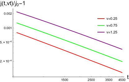
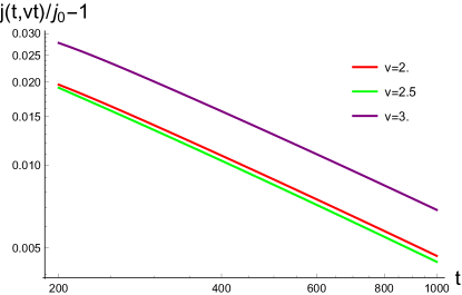
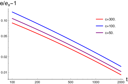
In section 4.3 we studied the numerical solutions to the Riemann problem for various initial energy and velocity profiles associated with , and type solutions. In what follows we provide additional evidence that at late times the full numerical solution to the Riemann problem approaches the appropriate predicted steady state values and and fixed point values and .
B.1 RR configurations
To generate an RR configuration we used the initial data
| (81) |
where
| (82) |
The analysis of section 4.2 predicts a steady state of the form
| (83) |
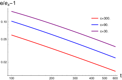
Once one should find a fixed point with . We find that the numerical solution approaches the predicted states via power law behavior, see figure 11.

B.2 SS configurations
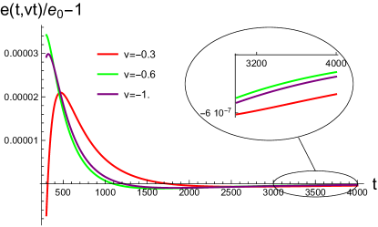
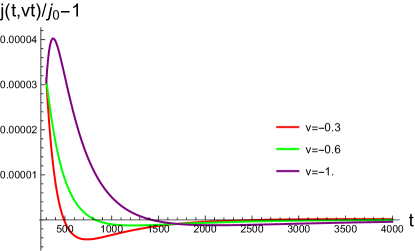
To generate an SS configuration we used the initial data (81) with . The analysis of section 4.2 predicts a steady state of the form
| (84) |
See figure 12 for a comparison with the numerical data.


B.3 RS configurations
To generate an RS configuration we used the initial data
| (85) |
where
| (86) |
The analysis of section 4.2 predicts a steady state of the form
| (87) |
with
| (88) |
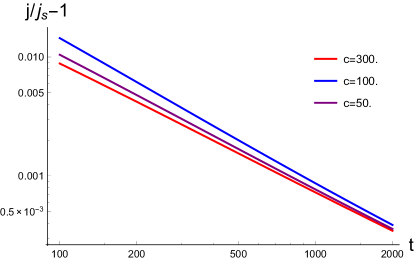
According to the same analysis, once we will obtain a fixed point at the origin with . An analysis of the late time behavior of the numerical solution can be found in figure 13.


B.4 Error analysis
In sections B.1 and B.3 we have fit the late time approach of the data to the predicted steady state and (or) fixed point values to a power law behavior. The fit was done using Mathematica’s NonLinearModelFit routine Mathematica . In detail, the late time data was discretized into order 1 time steps which were then fit to a curve with and as parameters. The standard errors for the fit were usually of order to . Fits involving very small values of the slope parameter in (82) and (86) (c.f., the bottom plots of figures 11 and 13) often had large standard errors.
References
- (1) R. Emparan, R. Suzuki and K. Tanabe, Evolution and End Point of the Black String Instability: Large D Solution, Phys. Rev. Lett. 115 (2015) 091102, [1506.06772].
- (2) J. Smoller, Shock Waves and Reaction-Diffusion Equations. Springer-Verlag, 1982.
- (3) D. Bernard and B. Doyon, Energy flow in non-equilibrium conformal field theory, J. Phys. A45 (2012) 362001, [1202.0239].
- (4) D. Bernard and B. Doyon, Conformal field theory out of equilibrium: a review, 1603.07765.
- (5) H.-C. Chang, A. Karch and A. Yarom, An ansatz for one dimensional steady state configurations, J. Stat. Mech. 1406 (2014) P06018, [1311.2590].
- (6) X. Liu and Y. Oz, Shocks and Universal Statistics in (1+1)-Dimensional Relativistic Turbulence, JHEP 03 (2011) 006, [1006.0494].
- (7) M. J. Bhaseen, B. Doyon, A. Lucas and K. Schalm, Far from equilibrium energy flow in quantum critical systems, 1311.3655.
- (8) I. Amado and A. Yarom, Black brane steady states, JHEP 10 (2015) 015, [1501.01627].
- (9) E. Megias, Out-of-equilibrium energy flow and steady state configurations in AdS/CFT, PoS EPS-HEP2015 (2015) 366, [1510.04219].
- (10) I. Bakas, K. Skenderis and B. Withers, Self-similar equilibration of strongly interacting systems from holography, 1512.09151.
- (11) R. Pourhasan, Non-equilibrium steady state in the hydro regime, JHEP 02 (2016) 005, [1509.01162].
- (12) A. Lucas, K. Schalm, B. Doyon and M. J. Bhaseen, Shock waves, rarefaction waves and non-equilibrium steady states in quantum critical systems, 1512.09037.
- (13) M. Spillane and C. P. Herzog, Relativistic Hydrodynamics and Non-Equilibrium Steady States, 1512.09071.
- (14) R. Emparan, K. Izumi, R. Luna, R. Suzuki and K. Tanabe, Hydro-elastic Complementarity in Black Branes at large D, 1602.05752.
- (15) S. Bhattacharyya, A. De, S. Minwalla, R. Mohan and A. Saha, A membrane paradigm at large D, 1504.06613.
- (16) S. Bhattacharyya, M. Mandlik, S. Minwalla and S. Thakur, A Charged Membrane Paradigm at Large D, 1511.03432.
- (17) R. Emparan, R. Suzuki and K. Tanabe, The large D limit of General Relativity, JHEP 06 (2013) 009, [1302.6382].
- (18) R. Emparan, D. Grumiller and K. Tanabe, Large-D gravity and low-D strings, Phys. Rev. Lett. 110 (2013) 251102, [1303.1995].
- (19) R. Emparan and K. Tanabe, Holographic superconductivity in the large D expansion, JHEP 01 (2014) 145, [1312.1108].
- (20) R. Emparan and K. Tanabe, Universal quasinormal modes of large D black holes, Phys. Rev. D89 (2014) 064028, [1401.1957].
- (21) R. Emparan, R. Suzuki and K. Tanabe, Instability of rotating black holes: large D analysis, JHEP 06 (2014) 106, [1402.6215].
- (22) R. Emparan, R. Suzuki and K. Tanabe, Decoupling and non-decoupling dynamics of large D black holes, JHEP 07 (2014) 113, [1406.1258].
- (23) R. Emparan, R. Suzuki and K. Tanabe, Quasinormal modes of (Anti-)de Sitter black holes in the 1/D expansion, JHEP 04 (2015) 085, [1502.02820].
- (24) T. Andrade, S. A. Gentle and B. Withers, Drude in D major, 1512.06263.
- (25) A. M. Garcia-Garcia and A. Romero-Bermudez, Conductivity and entanglement entropy of high dimensional holographic superconductors, JHEP 09 (2015) 033, [1502.03616].
- (26) S. Bhattacharyya, V. E. Hubeny, S. Minwalla and M. Rangamani, Nonlinear Fluid Dynamics from Gravity, JHEP 02 (2008) 045, [0712.2456].
- (27) M. Haack and A. Yarom, Nonlinear viscous hydrodynamics in various dimensions using AdS/CFT, JHEP 10 (2008) 063, [0806.4602].
- (28) S. Bhattacharyya, R. Loganayagam, I. Mandal, S. Minwalla and A. Sharma, Conformal Nonlinear Fluid Dynamics from Gravity in Arbitrary Dimensions, JHEP 12 (2008) 116, [0809.4272].
- (29) S. Grozdanov and N. Kaplis, Constructing higher-order hydrodynamics: The third order, 1507.02461.
- (30) S. Bhattacharyya, V. E. Hubeny, R. Loganayagam, G. Mandal, S. Minwalla, T. Morita et al., Local Fluid Dynamical Entropy from Gravity, JHEP 06 (2008) 055, [0803.2526].
- (31) D. T. Son and P. Surowka, Hydrodynamics with Triangle Anomalies, Phys. Rev. Lett. 103 (2009) 191601, [0906.5044].
- (32) P. M. Chesler and L. G. Yaffe, Boost invariant flow, black hole formation, and far-from-equilibrium dynamics in N = 4 supersymmetric Yang-Mills theory, Phys. Rev. D82 (2010) 026006, [0906.4426].
- (33) P. M. Chesler and L. G. Yaffe, Holography and colliding gravitational shock waves in asymptotically spacetime, Phys. Rev. Lett. 106 (2011) 021601, [1011.3562].
- (34) P. M. Chesler and L. G. Yaffe, Numerical solution of gravitational dynamics in asymptotically anti-de Sitter spacetimes, JHEP 07 (2014) 086, [1309.1439].
- (35) K. Balasubramanian and C. P. Herzog, Losing Forward Momentum Holographically, Class. Quant. Grav. 31 (2014) 125010, [1312.4953].
- (36) P. M. Chesler, N. Kilbertus and W. van der Schee, Universal hydrodynamic flow in holographic planar shock collisions, JHEP 11 (2015) 135, [1507.02548].
- (37) S. Khlebnikov, M. Kruczenski and G. Michalogiorgakis, Shock waves in strongly coupled plasmas, Phys. Rev. D82 (2010) 125003, [1004.3803].
- (38) E. Shuryak, Shocks in Quark-Gluon Plasmas, Phys. Rev. C86 (2012) 024907, [1203.6614].
- (39) S. Fischetti, D. Marolf and J. E. Santos, AdS flowing black funnels: Stationary AdS black holes with non-Killing horizons and heat transport in the dual CFT, Class. Quant. Grav. 30 (2013) 075001, [1212.4820].
- (40) P. Figueras and T. Wiseman, Stationary holographic plasma quenches and numerical methods for non-Killing horizons, Phys. Rev. Lett. 110 (2013) 171602, [1212.4498].
- (41) R. Emparan and M. Martinez, Black String Flow, JHEP 09 (2013) 068, [1307.2276].
- (42) Wolfram Research Inc., Mathematica, 2016.
- (43) A. H. Taub, Relativistic Rankine-Hugoniot equations, Physical Review 74.3 (1948) 328.
- (44) K. W. Thomson, The special relativistic shock tube, Journal of Fluid Mechanics 171 (1986) 365–375.
- (45) P. Mach and M. Pietka, Exact solution of the hydrodynamical riemann problem with nonzero tangential velocities and the ultrarelativistic equation of state, Physical Review (2010) 046313, [0905.0349].
- (46) P. Mach, Corrugation instabilities of the riemann problem in relativistic hydrodynamics, 1104.3751.
- (47) S. S. Gubser, Breaking an Abelian gauge symmetry near a black hole horizon, Physical Review D78 (2008) 065034, [0801.2977].
- (48) S. A. Hartnoll, C. P. Herzog and G. T. Horowitz, Building a Holographic Superconductor, Phys. Rev. Lett. 101 (2008) 031601, [0803.3295].
- (49) S. A. Hartnoll, C. P. Herzog and G. T. Horowitz, Holographic Superconductors, JHEP 12 (2008) 015, [0810.1563].
- (50) C. P. Herzog, P. K. Kovtun and D. T. Son, Holographic model of superfluidity, Phys. Rev. D79 (2009) 066002, [0809.4870].
- (51) C. P. Herzog, N. Lisker, P. Surowka and A. Yarom, Transport in holographic superfluids, JHEP 08 (2011) 052, [1101.3330].