Squares that Look Round: Transforming Spherical Images

Abstract

We propose Möbius transformations as the natural rotation and scaling tools for editing spherical images. As an application we produce spherical Droste images. We obtain other self-similar visual effects using rational functions, elliptic functions, and Schwarz-Christoffel maps.

Introduction

Interest in spherical imagery has grown in recent years, driven by increased availability of both viewing devices and cameras. The YouTube application on smartphones now plays spherical video, using the phone’s accelerometer. On the camera side, numerous consumer-focused spherical cameras are available, as well as high-end professional offerings.

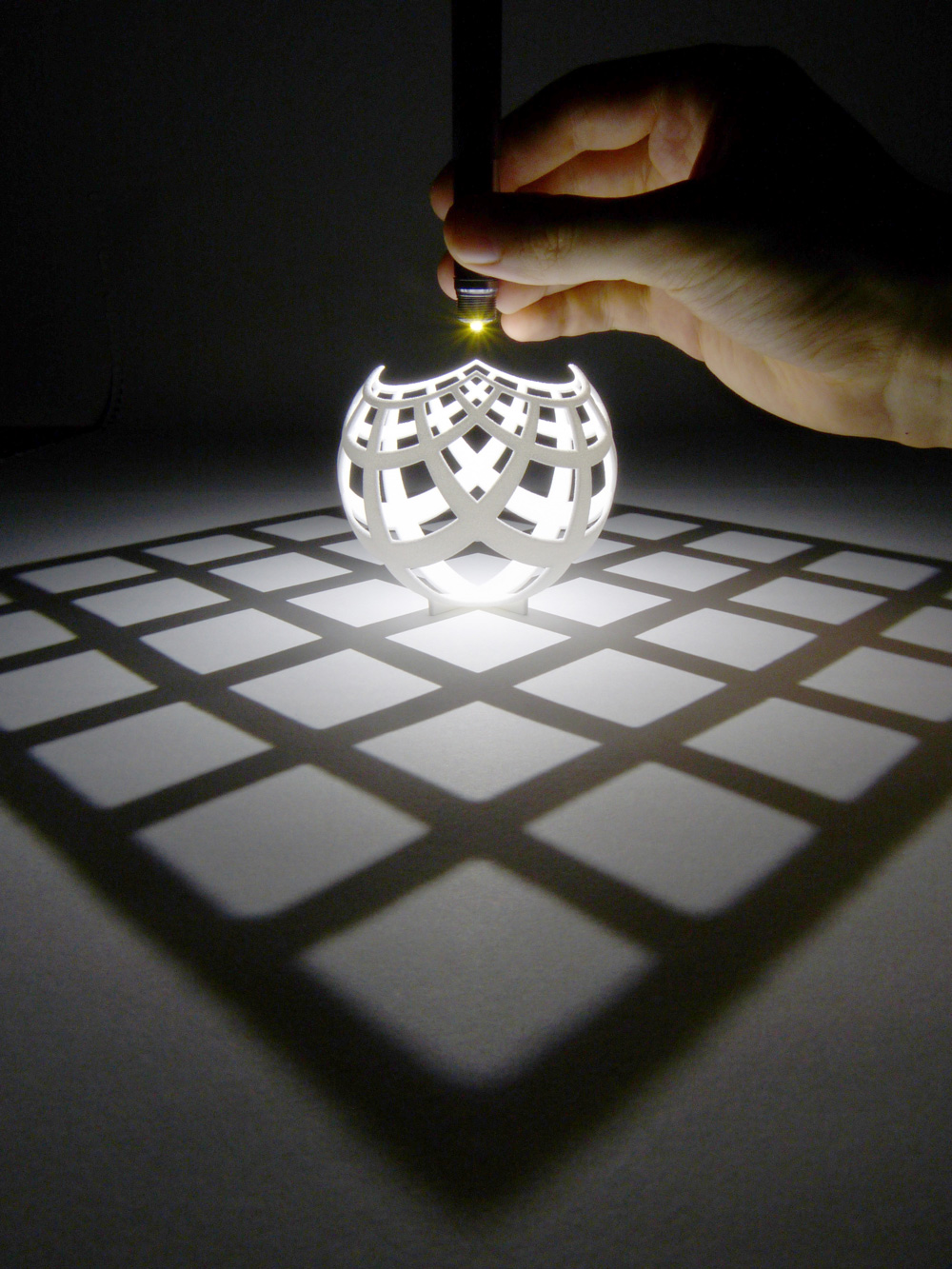
Figure 1: Stereographic projection from the sphere to the plane.

Almost universally, spherical images and video are stored and transmitted via equirectangular projection: points on the sphere are given by their latitude and longitude. Thus the whole image is stored as a rectangular image with a two-to-one aspect ratio, corresponding to angles $(0,2\pi)\times(-\pi/2,\pi/2)$. This data format fits conveniently into the existing infrastructure for ordinary images. However, there is a problem: most tools for editing ordinary rectangular images, when applied to the equirectangular projection, give poor results. For example, standard rectangular editing tools cannot rotate a spherical image about a non-vertical axis.

Future editing tools for spherical images will no doubt include the ability to rotate images around any axis, giving analogues of both translation and rotation of flat images. However, we can also ask what scaling (in video, zooming) might mean for spherical images. In this paper, we first recall how Möbius transformations naturally rotate and scale the sphere. We then use these to produce spherical Droste images. We also obtain other interesting visual effects using rational functions, elliptic functions, and Schwarz-Christoffel maps.

Acknowledgements: The second author was inspired by a paper of Sébastien Pérez-Duarte and David Swart [10]. See also [4]. He began work whilst visiting eleVR (a research group consisting of Emily Eifler, Vi Hart and Andrea Hawksley) and wrote a guest blog post explaining the implementation of Möbius transformations. The Python code used to generate many of these images is available at GitHub. All spherical photographs and videos were taken using a Ricoh Theta S.

Möbius transformations

Möbius transformations act on the Riemann sphere, $\widehat{\mathbb{C}}=\mathbb{C}\cup\{\infty\}$. This is the result of adding a single point, $\infty$, to the complex plane $\mathbb{C}$. We map from the unit sphere $S^{2}$ in $\mathbb{R}^{3}$ to the Riemann sphere using stereographic projection [8, page 57]:

$$\rho(u,v,w)=\frac{u+iv}{1-w}$$

We set $\rho(0,0,1)=\infty$. Every other point of the unit sphere maps to a point of $\mathbb{C}$. Figure 1 shows a 3D printed visualisation of stereographic projection. A Möbius transformation $M=(a,b;c,d)$ is the map from the Riemann sphere to itself given by

$$M(z)=\frac{az+b}{cz+d},\quad\mbox{where $a,b,c,d\in\mathbb{C}$ and $ad-bc\neq 0$.}$$

There are various special cases involving the point at infinity. If $cz+d=0$ then $M(z)=\infty$. If $c\neq 0$ then $M(\infty)=a/c$. If $c=0$ then $M(\infty)=\infty$. There is a cleaner definition, avoiding these special cases, which uses the one-dimensional complex projective space $\mathbb{CP}^{1}$ which we use in our implementation. Here, to simplify the exposition, we use $\widehat{\mathbb{C}}$.

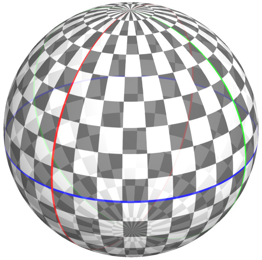
(a)

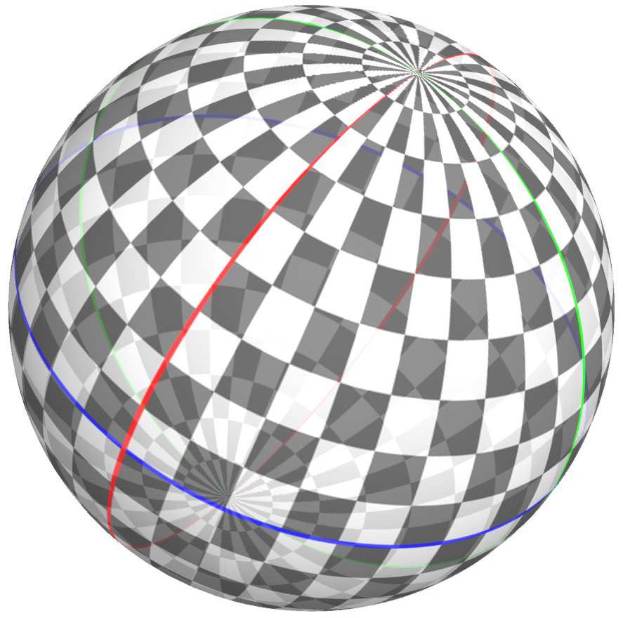
(b)

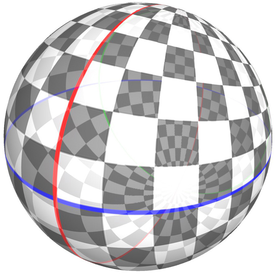
(c)

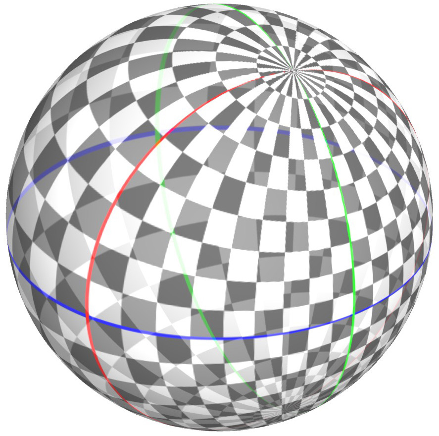
(d)

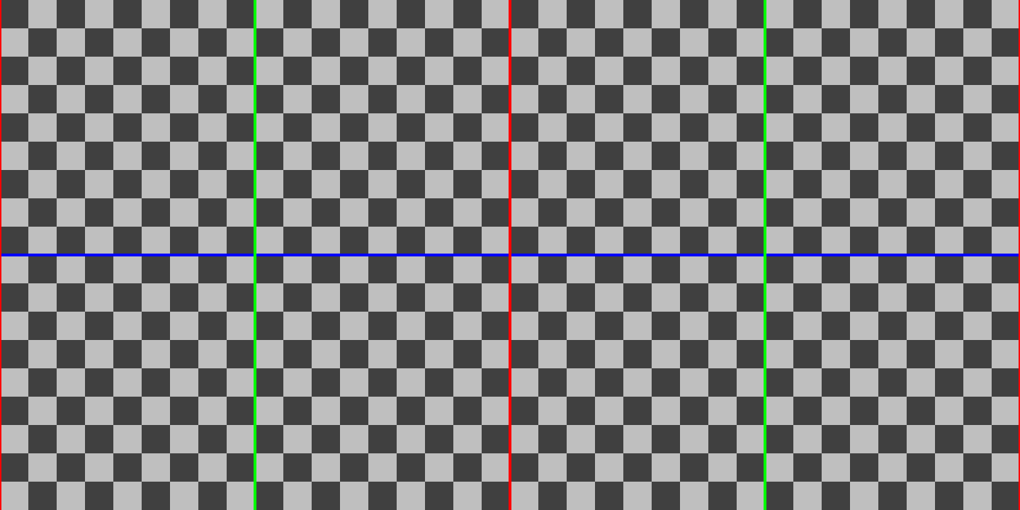
(e)

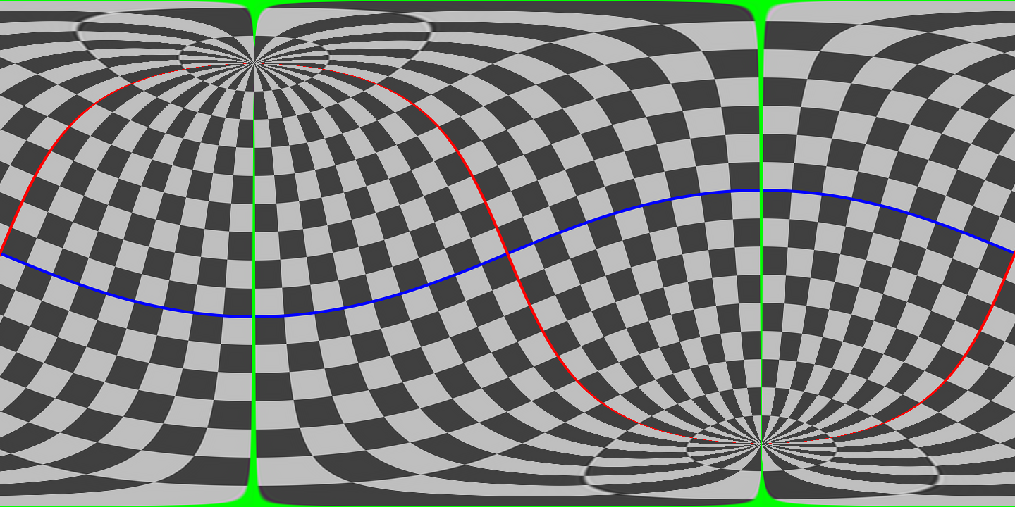
(f)

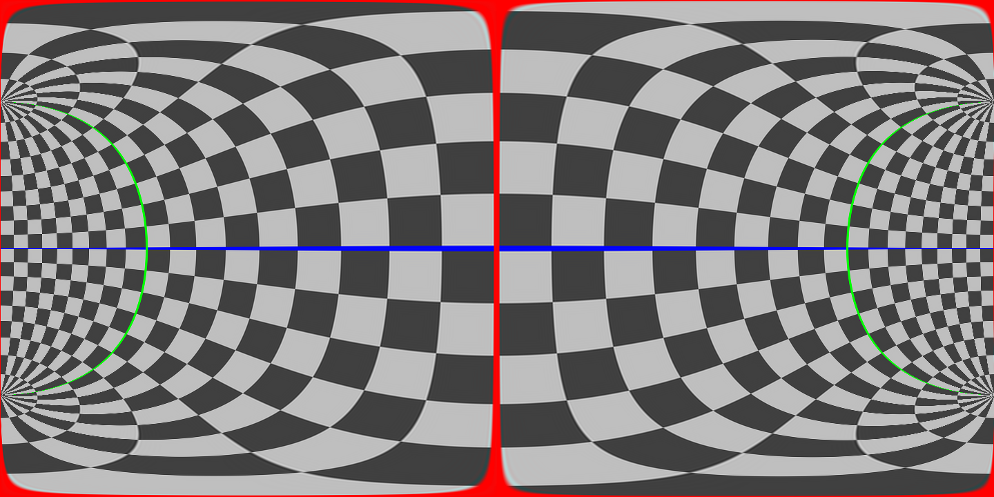
(g)

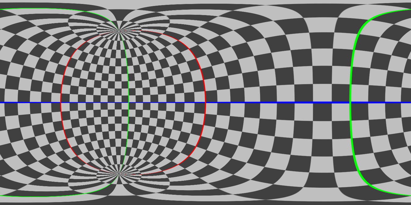
(h)

Figure 2: A test pattern (a and e), and the results of rotating by $\pi/8$ (b and f), scaling by a factor of two (c and g) and applying the parabolic translation $M(z)=z+1/2$ (d and h). Above: the textures on the sphere. Below: their equirectangular projections. Note that we generally view a spherical image from inside the sphere. From this perspective the equirectangular projections have the same orientation as the textures on the spheres.

We can rotate the complex plane about $0$ by multiplying by a unit complex number, say $e^{i\theta}$. We can scale the plane, again centered on $0$, by multiplying by a real number, say $\lambda\in\mathbb{R}$. Finally, we can translate the plane by adding a complex number, say $w$. These give $M=(e^{i\theta},0;0,1)$ (elliptic), $M=(\lambda,0;0,1)$ (hyperbolic), and $M=(1,w;0,1)$ (parabolic). Every Möbius transformation is equivalent, via conjugation, to one of these.

Figure 2 (top row) shows an initial test pattern, and the results of applying a rotation by $\theta=\pi/8$, of scaling by a factor of $\lambda=2$, and of adding $w=1/2$. The parabolic case is included for completeness; it is not clear how this might be used in image editing. Here we have placed zero, the origin of the complex plane, at the “front pole” of the sphere: the front intersection of the blue equator and red longitude. Note how the hyperbolic transformation scales distances up by a factor of two at zero but scales distances down by a factor of two at the antipodal point, $\infty$. In fact, Möbius transformations allow us to rotate or scale fixing any two points of the sphere. As an example, see Figure 3; we show a frame of raw footage and the transformed frame from a video exploring many of the effects in this paper.

Every Möbius transformation, other than rotations about antipodal points, distorts spherical distance. However, as illustrated in Figure 2, right angles always remain right angles. In fact, Möbius transformations are conformal: they preserve all angles. Thus images are not sheared or non-uniformly stretched; features remain essentially recognisable. All of the transformations in this paper mapping the sphere to itself are conformal, apart from at a discrete set of points. Note that the equirectangular projection is not conformal; both distances and angles are distorted.

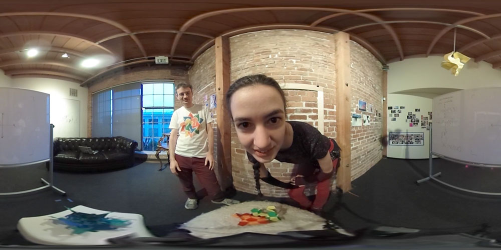
(a) The input image.

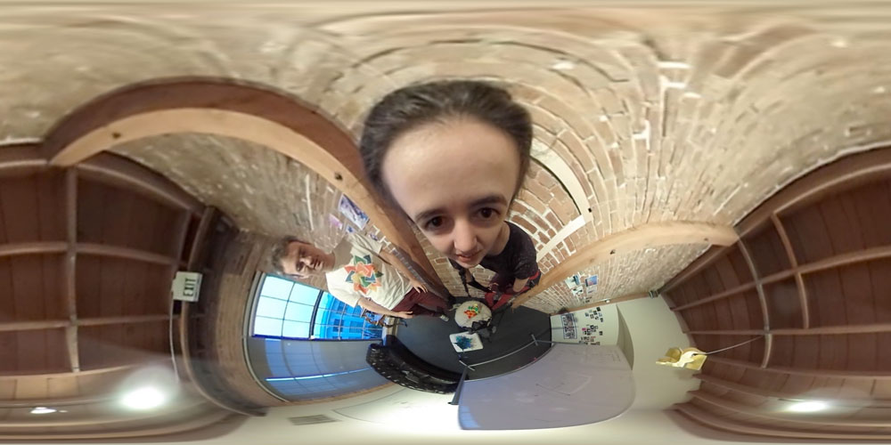
(b) The result of rotating by an angle of $\pi/12$.

Figure 3: Rotating a spherical photograph of Vi Hart and Henry Segerman, about Vi’s eyes.

Pulling back, pushing forward, and branch points

If we want to apply a transformation $T$ to a pixel-based input image $\mathcal{I}_{\text{in}}$, we need to find the inverse transformation $S=T^{-1}$. This is because the algorithm to generate the output image $\mathcal{I}_{\text{out}}$ runs in reverse: for each desired pixel $p$ of $\mathcal{I}_{\text{out}}$, we take its position $z_{p}$, compute $S(z_{p})$, and assign $p$ the same color as the pixel with position $S(z_{p})$ in $\mathcal{I}_{\text{in}}$. (In fact we take a weighted average of colors of input pixels nearest to $S(z_{p})$.) Note that, in order to have an algorithm, the transformation $S=T^{-1}$ must be single-valued, but $T$ need not be. We call this procedure pulling back via $S$ or, equivalently, pushing forward via $T$.

(a) The input image.

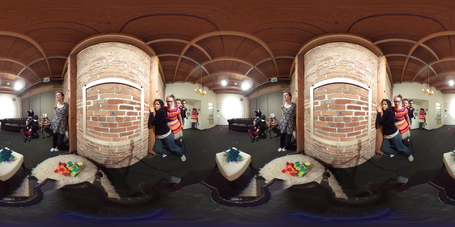
(b) Pulling back by $S(z)=z^{2}$.

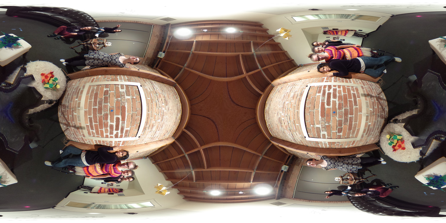
(c) Rotated to show an order two branch point at the center.

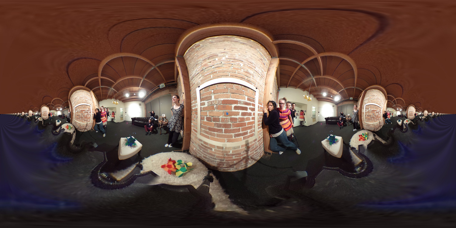
(d) Pulling back via $S(z)=-e^{-4\left(\frac{1+z}{1-z}\right)}$.

Figure 4: Transformations applied to a spherical photograph featuring Emily Eifler, Vi Hart, Andrea Hawksley, and Henry Segerman, all appearing twice. In these images the origin $0\in\mathbb{C}$ corresponds to the top of the equirectangular projection while infinity corresponds to the bottom, other than for Figure 4c.

Now consider Figure 4a. If we take $T(z)=\pm\sqrt{z}$ and $S(z)=z^{2}$ then we obtain Figure 4b. Here we see a new feature, branch points, around which nearby imagery is repeated. To see the branch point more clearly, we rotate Figure 4b to get Figure 4c. The number of repetitions is the order of a branch point. In $\widehat{\mathbb{C}}$ the branch points are of order two and lie at zero and infinity. In Figures 4b and 4c they are on the floor and the ceiling. These branch points are unavoidable: any conformal transformation of $\widehat{\mathbb{C}}$ is either a Möbius transformation or has branch points [2, Section 4.3.2].

Figure 4d shows the result of pulling back via a variant of the complex exponential map, specifically $S(z)=-e^{-\lambda\left(\frac{1+z}{1-z}\right)}$. Here $\lambda$ is a scaling parameter and the Möbius transformation $M(z)=\frac{1+z}{1-z}$ is a rotation by $\pi/2$ about $\pm i$; this ensures that the image repeats horizontally rather than vertically. In this case, the forward transformation $T(z)$ is a variant of the complex logarithm, so is infinitely valued. Thus the output contains infinitely many copies of the input image. The branch points are again on the floor and the ceiling, but are of infinite order.

The same techniques can be used to combine different spherical images into a single spherical image. This provides a spherical analogue of the familiar “split screen” trope in rectangular video: compositing multiple video clips into a single screen. We, however, can stitch the different images seamlessly, if they match along suitable arcs between the branch points. We created a spherical video along these lines, in which the second author appears to be in a two-fold branched cover of his apartment. The footage is stitched together with a video of the empty apartment, so that only one copy of the author appears in the combined video.

The Droste effect

(a) A Droste annulus.

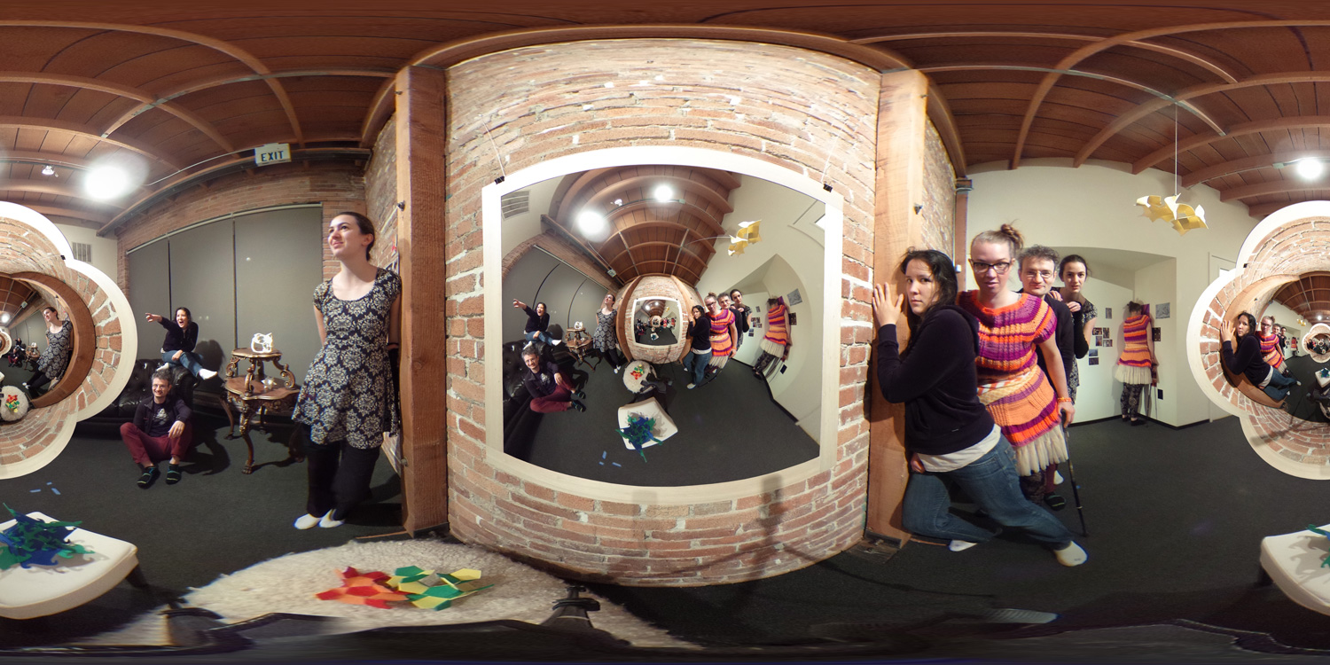
(b) A straight Droste image.

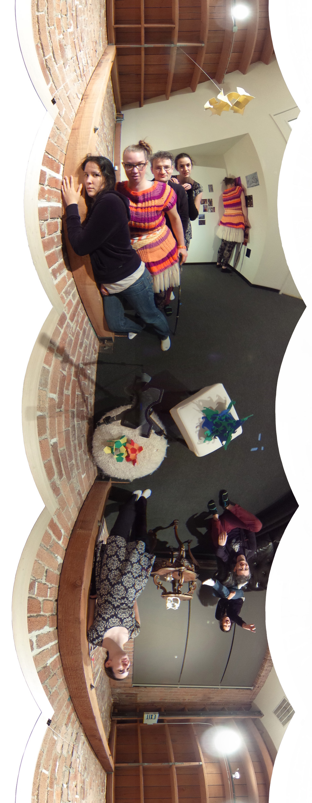
(c) Log of the Droste annulus.

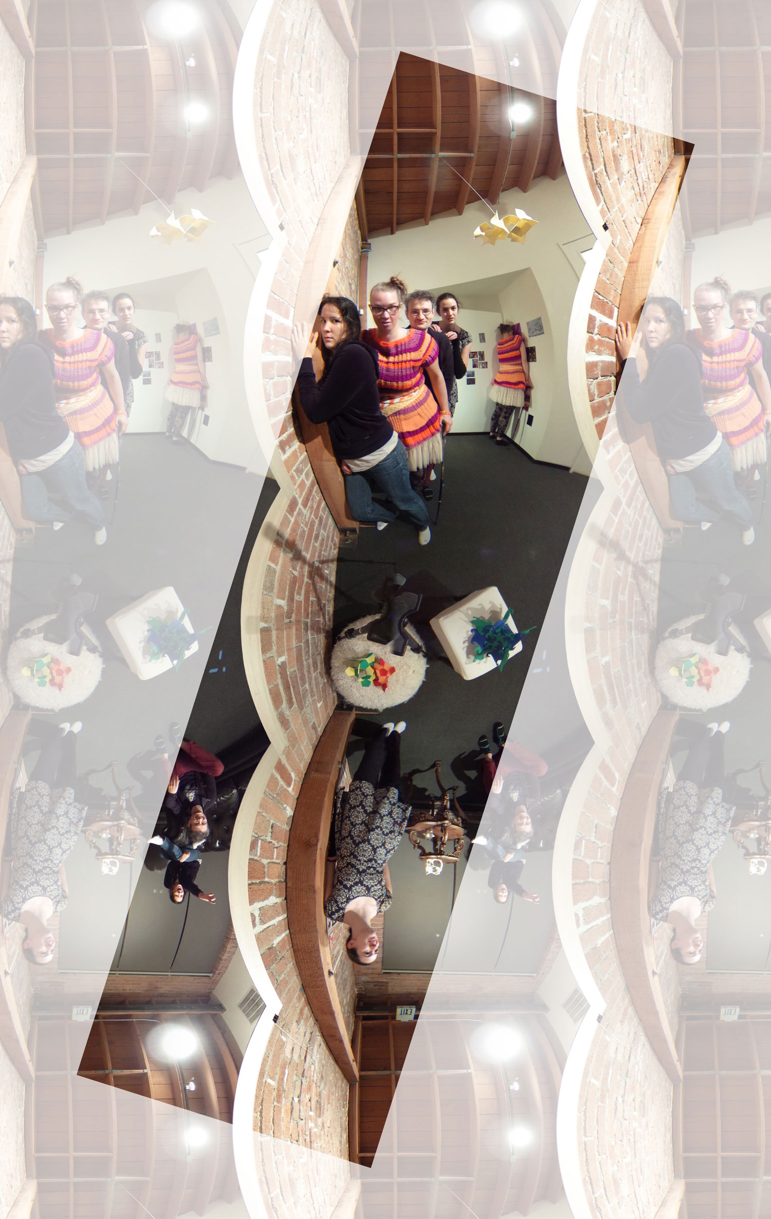
(d) A different fundamental rectangle.

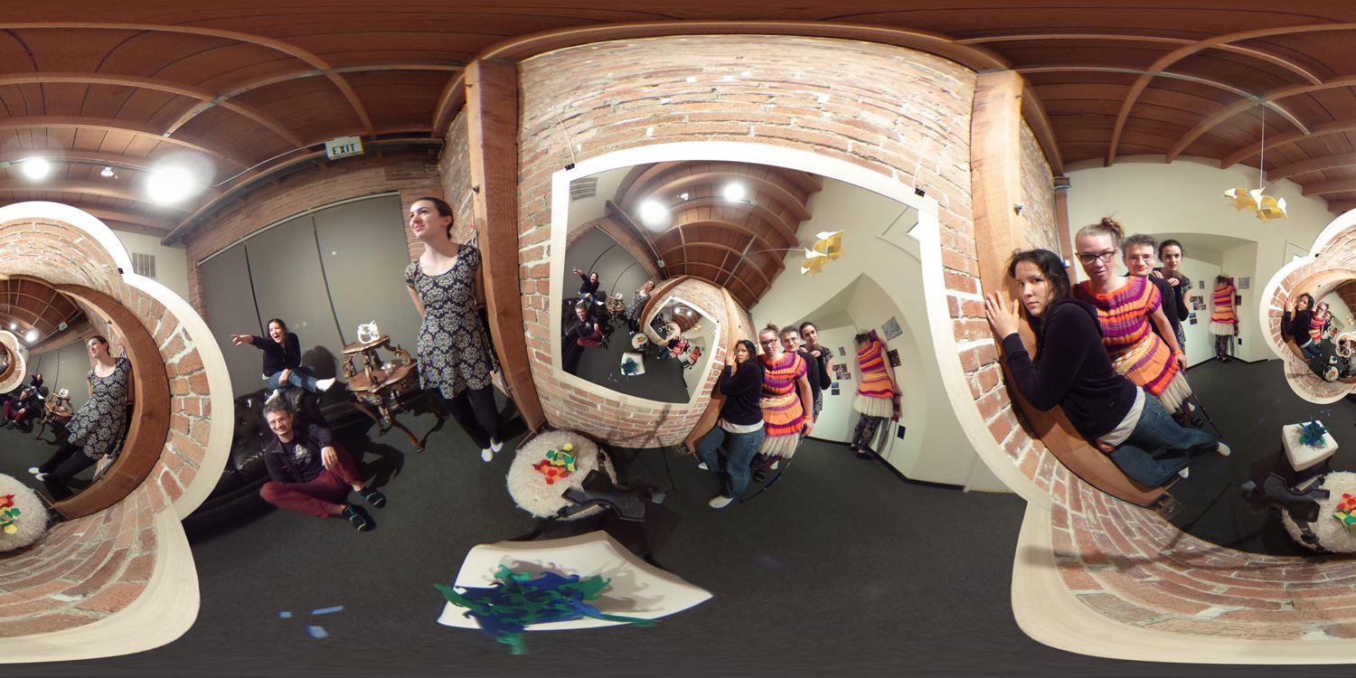
(e) A twisted Droste image.

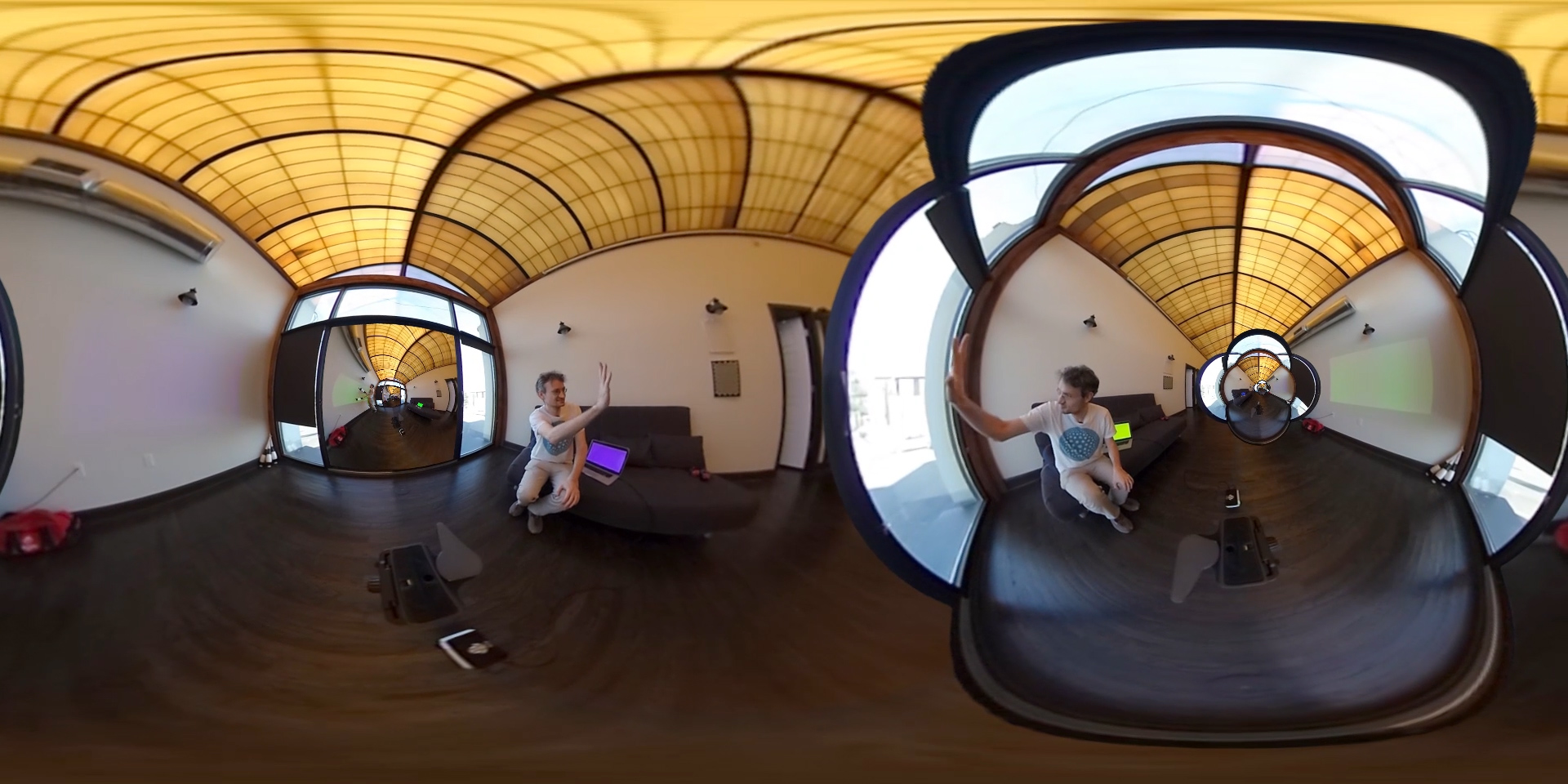
(f) Here the image inside the frame differs from the one outside.

Figure 5: Droste effect images. These images answer the question of what an observer inside of a Droste effect image sees when they look away from the frame: there is a flower-shaped portal floating in the middle of the room.

A common artistic and mathematical motif is that of “self-similarity”; this is often called the Droste effect in commercial and computer graphics. A “straight Droste effect”, as found on the packaging of the eponymous Dutch cocoa, is obtained when the entire picture is included, under a shrinking transformation, inside of itself. The “twisted Droste effect” was first introduced by M.C. Escher in his Print Gallery lithograph. The mathematics behind Escher’s image was explained by Bart de Smit and Hendrik Lenstra [3].

It is possible to obtain both the straight and twisted Droste effect in spherical images using Möbius transformations, the complex exponential map, and the complex logarithm (see also [10, page 223]). We simplify the discussion here by suppressing all mention of equirectangular and stereographic projections. We begin with a spherical image, say Figure 4a. We remove everything inside a small disk (here the inside of the frame on the wall) and everything outside a larger disk, to obtain a Droste annulus; see Figure 5a. We arrange matters so that there is a scaling transformation $M(z)=\lambda z$ that takes the outer boundary of the annulus to the inner boundary. Thus we may tile the sphere (minus two points) by copies of the annulus, obtaining a straight Droste image; see Figure 5b.

Applying a logarithm unwraps the Droste annulus to give an infinite vertical strip in $\mathbb{C}$ with width $\log\lambda$; see Figure 5c. Another way to obtain the straight Droste effect is to tile the plane by horizontal translations of the strip and apply the exponential map. Instead, we may follow De Smit and Lenstra [3, Figure 10], and obtain a twisted Droste effect. We scale and rotate so that the rectangle shown in Figure 5d is vertical and has height $2\pi$. Applying the exponential map yields Figure 5e.

Figure 5f shows a still image from a straight Droste videohttps://www.youtube.com/watch?v=qvh-EAipIUk in which different Droste annuli are offset in time as well as in space. The video is continually scaled, giving the impression of movement through the window. The time offset between neighboring annuli matches the apparent flight time of the camera; thus the video loops.

All constructions of Droste effect images seem to involve “cut-and-paste” techniques; here we had the choice of frame and the choice of scaling. In contrast, the pullback techniques of the previous section can be applied to any spherical image whatsoever. The output is seamless; the only blemishes are the branch points.

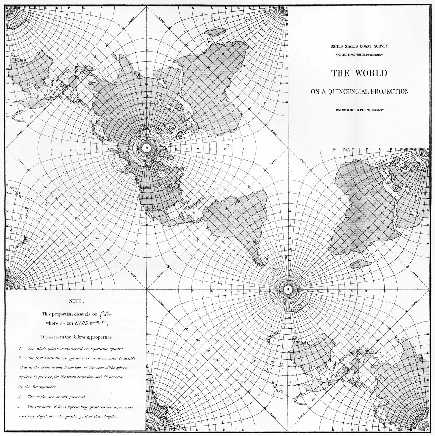
(a) Peirce’s quincuncial projection.

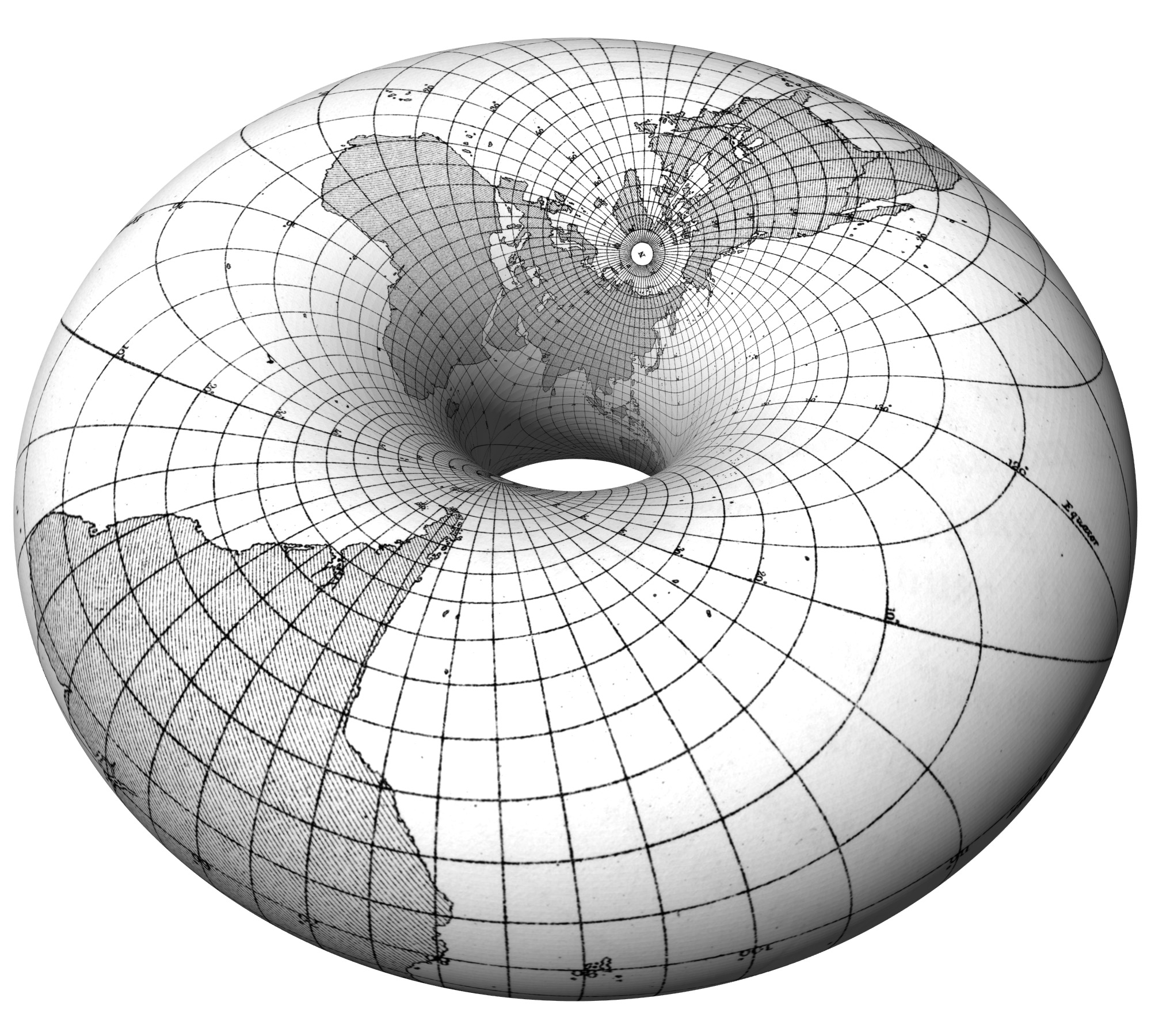
(b) On a torus, as in Figure 7a.

Figure 6:

Weierstrass and Schwarz-Christoffel

The exponential and logarithm are just two of the many beautiful flowers in the field of complex analysis. More exotic “elliptic” functions can be used; as far as we are aware, the earliest application to spherical images is due to Charles Sanders Peirce, in 1879 [9] (see also [1]). Figure 6a shows Peirce’s quincuncial projection; in Figure 6b we wrap it around the square torushttps://skfb.ly/NJRx.

Consider the Weierstrass $\wp$–function; we refer to [2, Chapter 7] for an excellent and short introduction. As a series the function for the square lattice is:

$$\wp_{i}(z)=\frac{1}{z^{2}}+\sideset{}{{}^{\prime}}{\sum}\left(\frac{1}{(z-w)^{2}}-\frac{1}{w^{2}}\right).$$

The sum ranges over the non-zero Gaussian integers $w\in\mathbb{Z}[i]$. It is a non-trivial exercise to check that $\wp_{i}(z+1)=\wp_{i}(z+i)=\wp_{i}(z)$. That is, the Weierstrass $\wp$–function is doubly periodic. In comparison, the exponential function is only singly periodic: $\exp(z+2\pi i)=\exp(z)$. The above series converges very slowly; for image processing we instead implement $\wp_{i}$ using theta-functions [6, page 132].

Since $\wp_{i}$ is doubly periodic, we think of it as first mapping the plane $\mathbb{C}$ to the square torus $\mathbb{T}$, which then maps to the Riemann sphere $\widehat{\mathbb{C}}$ via a branched double-cover. So, we start with our standard spherical image (Figure 7a, lefthttps://skfb.ly/NKox). We pullback to $\mathbb{T}$ and obtain a toroidal image (Figure 7a, righthttps://skfb.ly/NKpq). Note that the toroidal image contains two copies of the original, and has four branch points. Cutting $\mathbb{T}$ open we obtain Figure 7b; a square containing two copies of the original, spherical, image. This is the unit cell of a tiling of $\mathbb{C}$, obtained by pulling back via $\wp_{i}$.

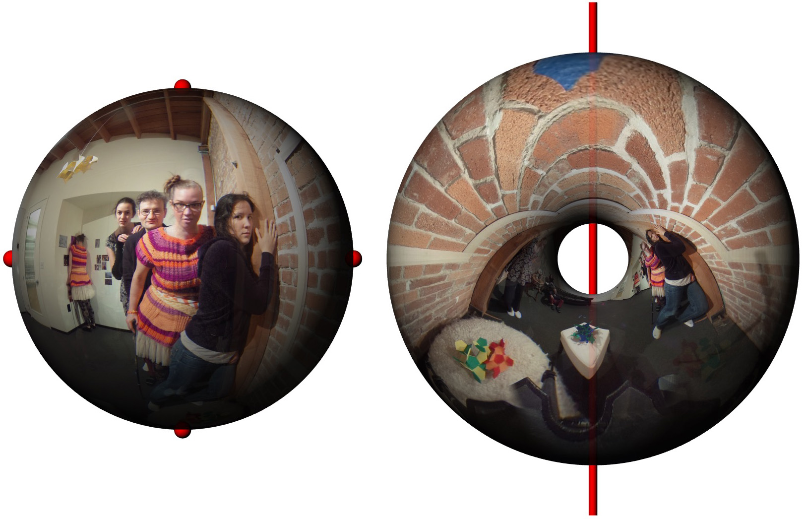
(a) The two-fold branched covering maps from the torus to the sphere by “folding” the torus around the red “skewer”. The four skewered points of the torus become the four red dots on the sphere.

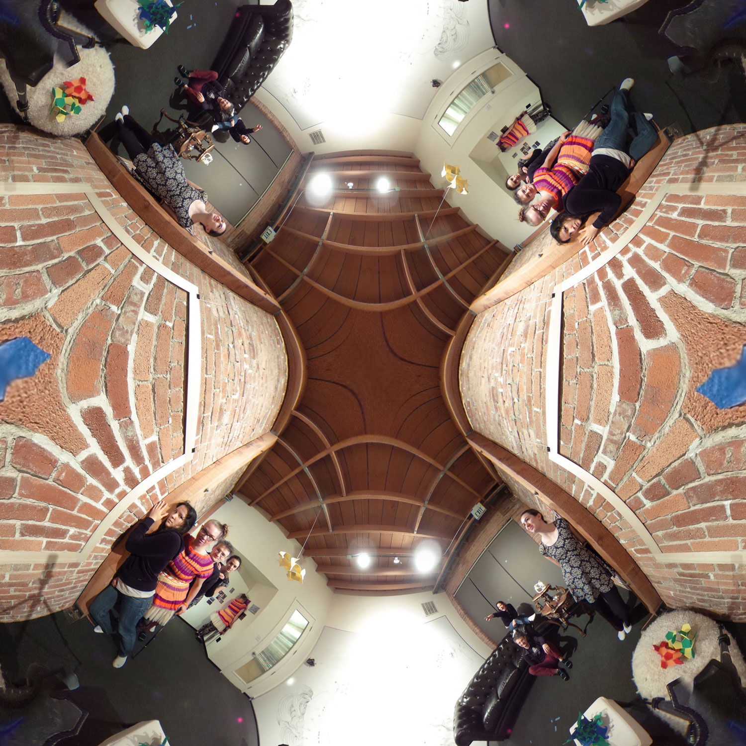
(b) Cutting open the torus yields a square that tiles the plane.

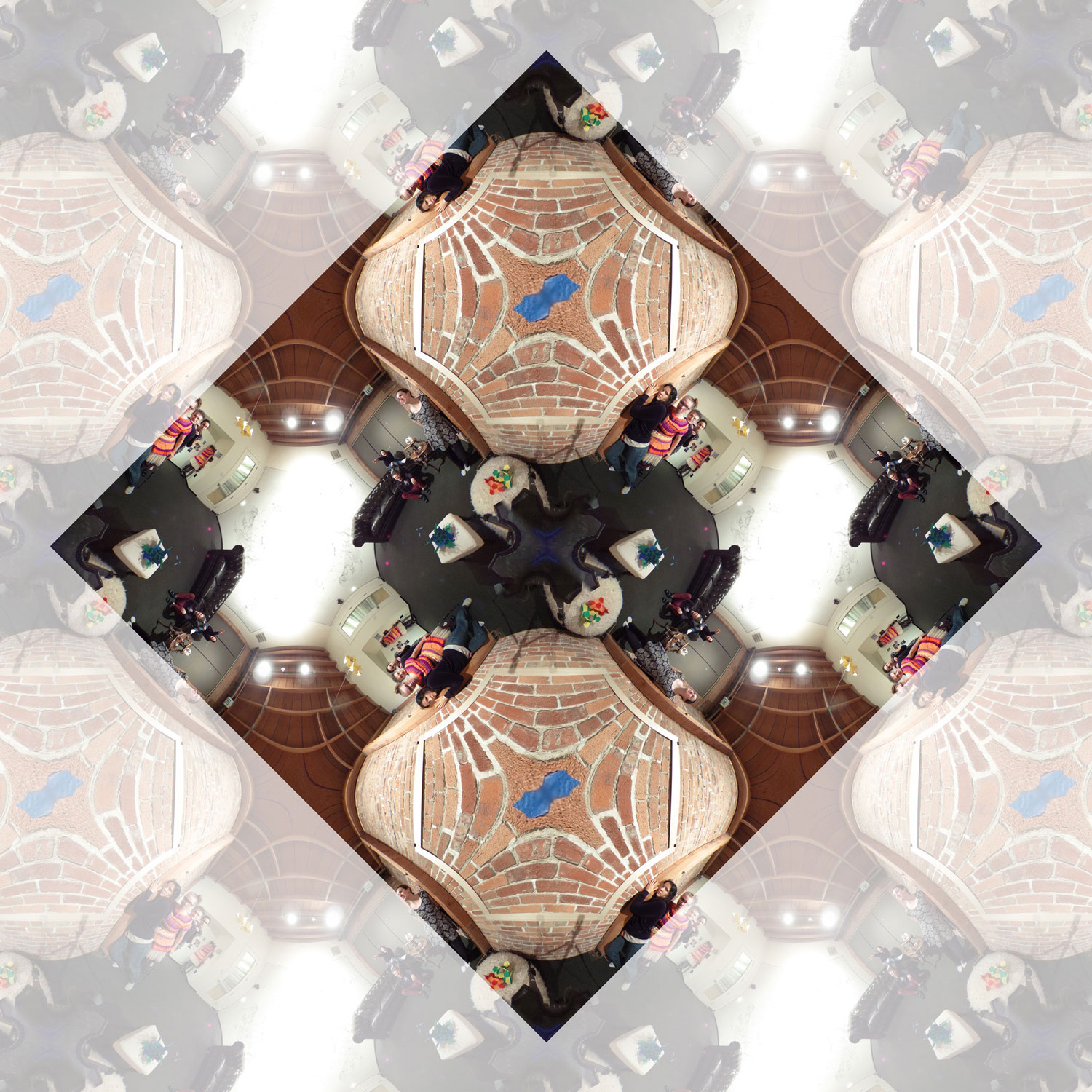
(c) A fundamental domain after rescaling by $z\mapsto(1+i)\cdot z$.

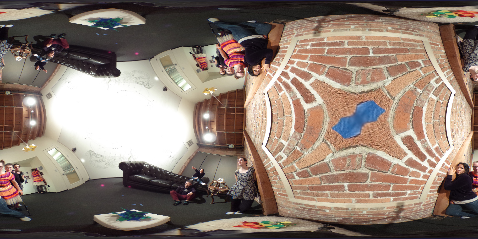
(d) Map down to the sphere again via Schwarz-Christoffel. The composition is the rational map $z\mapsto\frac{i}{2}(-z+1/z)$.

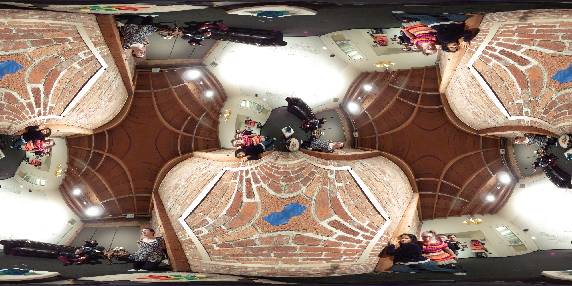
(e) The result if we instead use $z\mapsto 2\cdot z$. The corresponding rational function is $z\mapsto\frac{(z^{2}+1)^{2}}{4z(z^{2}-1)}$.

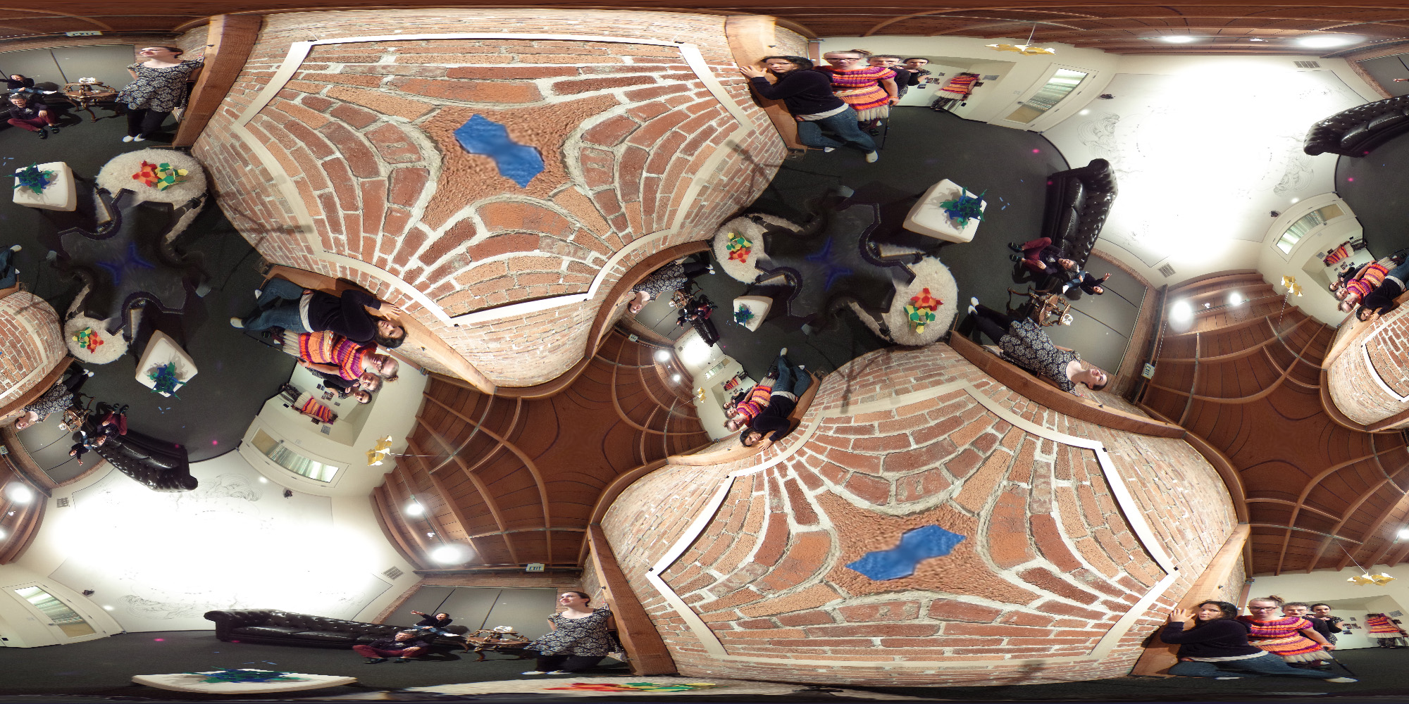
(f) The result if we instead use $z\mapsto(2+i)\cdot z$. Now we obtain the rational map $z\mapsto z\frac{((-1+2i)+z^{2})^{2}}{(-i+(2+i)z^{2})^{2}}$.

Figure 7: Images produced using Weierstrass and Schwarz-Christoffel maps.

Just as the exponential function has its logarithm, the Weierstrass function $\wp_{i}$ has an inverse. This map, denoted $\mathfrak{sc}_{4}$, takes the disk to the square. This, then, is a Schwarz-Christoffel function [2, Section 6.2.2]. In general, these functions are given by difficult integrals, but for regular $n$–gons there is a very pretty expression in terms of the hypergeometric function [5, Exercise 5.19]:

$$\mathfrak{sc}_{n}(z)=\int_{0}^{z}\frac{dw}{(1-w^{n})^{\frac{2}{n}}}=z\cdot{}_{2}F_{1}\left(\frac{1}{n},\frac{2}{n};1+\frac{1}{n};z^{n}\right).$$

We are now ready to “twist”, in similar spirit to the twisted Droste effect. We pullback the tiling in $\mathbb{C}$ via the map $z\mapsto(1+i)\cdot z$. A unit cell for this finer tiling is shown in Figure 7c. We pull this back to $\widehat{\mathbb{C}}$ using the map $\mathfrak{sc}_{4}$ and obtain Figure 7d. Pulling back (in $\mathbb{C}$) by other Gaussian integers gives other interesting effects; see Figures 7e, and 7f.

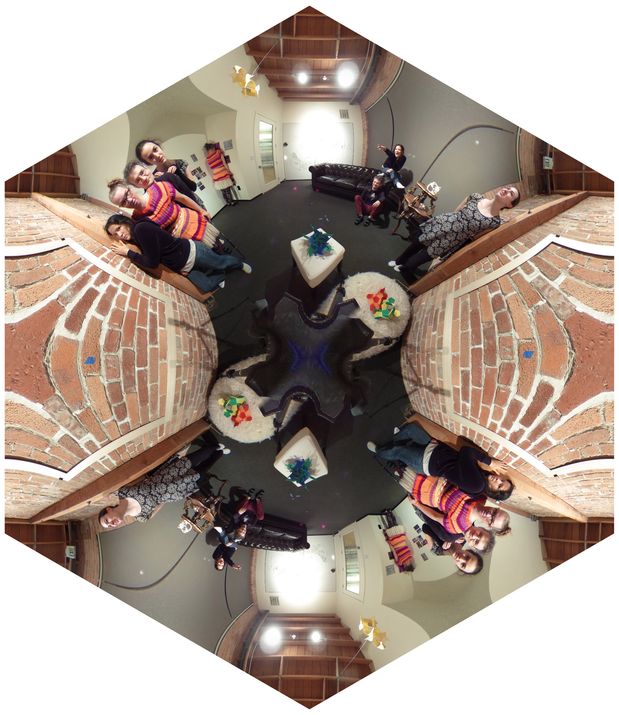
(a) Glue opposite sides to obtain the hexagonal torus.

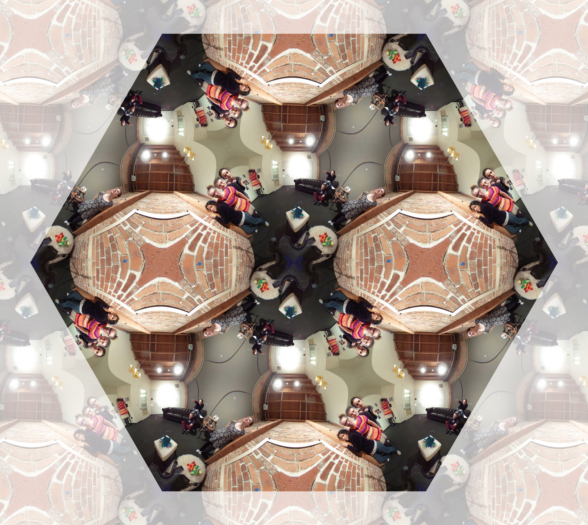
(b) A fundamental domain after rescaling by $z\mapsto(1+\omega)\cdot z$.

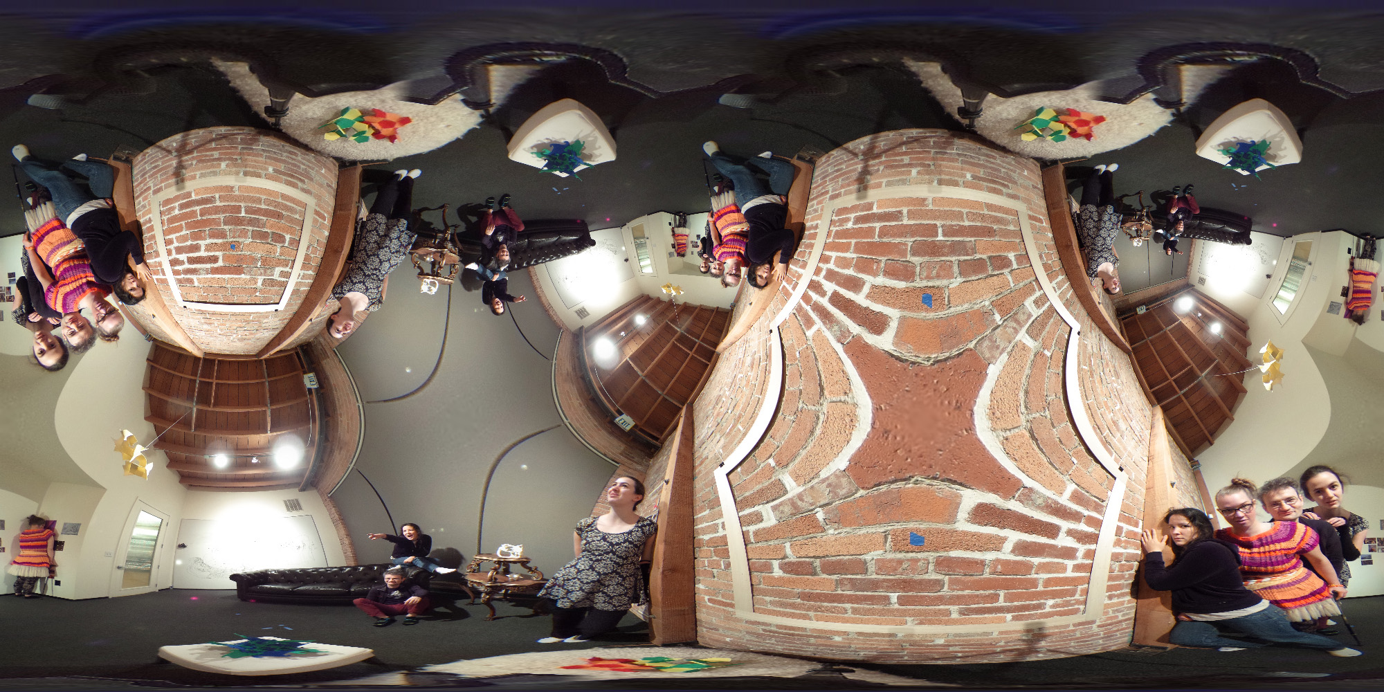
(c) The result of pulling up and pushing down is the rational function is $z\mapsto\frac{z^{3}+\sqrt{2}}{3\omega\cdot z^{2}}$.

Figure 8: Images produced with the hexagonal torus replacing the square torus.

It is well-known that gluing opposite sides of a square produces a torus. Less familiar is the fact that a torus also results from gluing opposite sides of a hexagon. We can now perform similar transformations to those above using the hexagonal torus. We pull our standard image Figure 4a back using the Weierstrass function $\wp_{\omega}$ where $\omega$ is the usual sixth root of unity – that is, the sum is over the lattice $\mathbb{Z}[\omega]$. We now pullback by $z\mapsto(1+\omega)z$ and then by the appropriate Schwarz-Christoffel function. See Figure 8.

In all cases the overall map from $\widehat{\mathbb{C}}$ to $\widehat{\mathbb{C}}$ is conformal, apart from a finite set of points. Thus it is in fact a rational map [2, Section 4.3.2]. It is far faster to use this rational function rather than the composition of elliptic and hypergeometric functions. It is possible to find the rational function synthetically [7, Chapter 7], but we found it simpler to proceed numerically, as follows. We must find the coefficients $\{a_{i},b_{i}\}$ of a rational function $f(z)=(\sum_{i=0}^{n}a_{i}z^{i})/(\sum_{i=0}^{n}b_{i}z^{i})$ of known degree $n$. Since $f$ is given above as a composition we can sample $f$ at a number of points $z_{j}$, getting the results $w_{j}=f(z_{j})$. Each sample gives a row

$$(z_{j}^{n},z_{j}^{n-1},\ldots,z_{j},1,-w_{j}z_{j}^{n},-w_{j}z_{j}^{n-1},\ldots,-w_{j}z_{j},-w_{j})$$

of a matrix $M$ with the property that $M\cdot(a_{n},a_{n-1},\ldots,a_{1},a_{0},b_{n},b_{n-1},\ldots,b_{1},b_{0})^{T}=0$. With enough samples, $M$ has a one-dimensional kernel, which can be found using the singular value decomposition method.

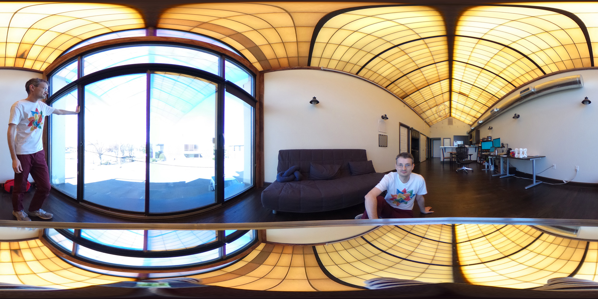
(a) The input image.

2pt $D_{a}$ at 1348 1385 $D_{A}$ at 3083 1479 $D_{b}$ at 2690 319 $D_{B}$ at 4436 2227

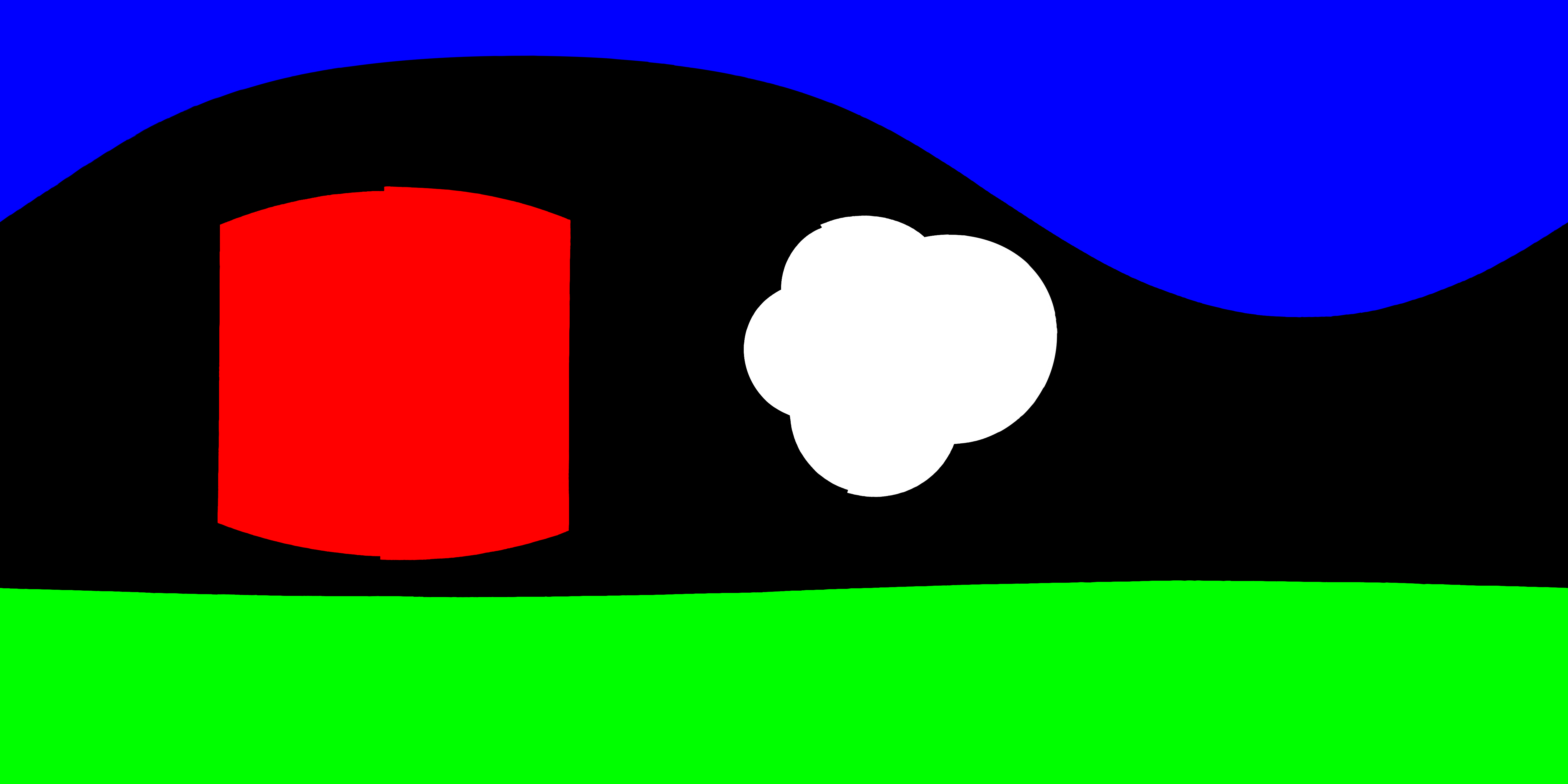
(b) The disks $D_{a}$, $D_{A}$, $D_{b}$, $D_{B}$ in the Riemann sphere.

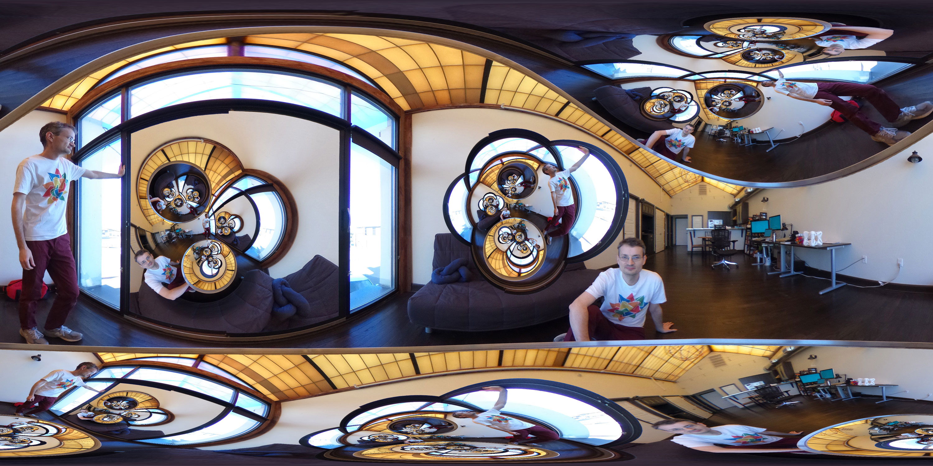
(c) A spherical Schottky image.

Figure 9: A spherical double Droste effect, using a Schottky group.

Schottky groups

Suppose that $a$ and $b$ are hyperbolic (that is, zooming) Möbius transformations. Suppose that $D_{a}$, $D_{A}$, $D_{b}$, $D_{B}$ are four closed disjoint disks in $\widehat{\mathbb{C}}$ so that $a$ maps the interior of $D_{A}$ onto the exterior of $D_{a}$, and similarly for $b$. Then the group generated by $a$ and $b$ is called a two-generator Schottky group [8, page 98].

Schottky groups can be used to generate impressive images; for a richly illustrated introduction to the underlying mathematics see [8]. David Gu has also experimented with applying Schottky reflection groups to photographs. We now discuss how to apply these ideas to spherical images.

We begin with an input image Figure 9a. We must choose the positions of the disks $D_{a}$, $D_{A}$, $D_{b}$, and $D_{A}$. In the final image these will contain zoomed copies of (part of) the input image. For $D_{a}$ we choose the window; for $D_{b}$ we choose the large round mirror lying below the camera, on which the tripod is standing. We trace over $D_{a}$ and $D_{b}$ in Photoshop to make a mask image in which the window is red and the mirror green, as shown in Figure 9b. We now choose two hyperbolic Möbius transformations, $A$ and $B$, and set $D_{A}=A(\widehat{\mathbb{C}}-D_{a})$, in white, and $D_{B}=B(\widehat{\mathbb{C}}-D_{b})$, in blue. We choose $A$ and $B$ so that the all of the disks are disjoint, and no disk covers an important part of the input image. Let $a=A^{-1}$ and define $b$ similarly.

To generate the image shown in Figure 9c, for each pixel $p$, we perform the following routine.

1. Set $q=p$.

2. If $q$ lies in the black region of the mask, color $p$ the same as the color of $q$ and stop the routine.

3. Otherwise, if $q$ lies in $D_{X}$ then replace $q$ by $x(q)$ and go to step $2$.

In general, a Schottky group can have more than two generators, or indeed fewer. Using just one generator recovers the straight Droste effect; $\widehat{\mathbb{C}}-(D_{a}\cup D_{A})$ is the Droste annulus. It is interesting to ponder how one might apply the twisted Droste effect throughout a Schottky image, but that is a task for another day.

References

- [1] Oscar S. Adams. Elliptic functions applied to conformal world maps. Department of Commerce U.S. Coast and Geodetic Survey. Govt. Print. Off., 1925. http://docs.lib.noaa.gov/rescue/cgs˙specpubs/QB275U35no1121925.pdf.
- [2] Lars V. Ahlfors. Complex analysis: An introduction of the theory of analytic functions of one complex variable. Second edition. McGraw-Hill Book Co., New York-Toronto-London, 1966.
- [3] Bart de Smit and Hendrik W. Lenstra Jr. The mathematical structure of Escher’s Print Gallery. Journal of the American Mathematical Society, 50(4):446–451, 2003. http://www.ams.org/notices/200304/fea-escher.pdf.
- [4] Daniel M. German, Pablo D’Angelo, Michael Gross, and Bruno Postle. New methods to project panoramas for practical and aesthetic purposes. In Computational Aesthetics’07 Proceedings of the Third Eurographics conference on Computational Aesthetics in Graphics, Visualization and Imaging, pages 15–22, 2007. http://turingmachine.org/~dmg/papers/dmg2007˙cae˙panos.pdf.
- [5] Jane M. McDougall, Lisbeth E. Schaubroeck, and James S. Rolf. Mappings to polygonal domains. In Explorations in complex analysis, Classr. Res. Mater. Ser., pages 271–315. Math. Assoc. America, Washington, DC, 2012. http://www.jimrolf.com/explorationsInComplexVariables/bookChapters/Ch5.pdf.
- [6] Henry McKean and Victor Moll. Elliptic curves. Cambridge University Press, Cambridge, 1997. Function theory, geometry, arithmetic.
- [7] John Milnor. Dynamics in One Complex Variable. Princeton University Press, 3rd edition, 2006.
- [8] David Mumford, Caroline Series, and David Wright. Indra’s pearls. Cambridge University Press, New York, 2002. The vision of Felix Klein.
- [9] Charles S. Peirce. A quincuncial projection of the sphere. Amer. J. Math., 2(4):394–396, 1879. https://www.jstor.org/stable/pdf/2369491.pdf.
- [10] Sébastien Pérez-Duarte and David Swart. The Mercator redemption. In Proceedings of Bridges 2013: Mathematics, Music, Art, Architecture, Culture, pages 217–224. Tessellations Publishing, 2013. http://archive.bridgesmathart.org/2013/bridges2013-217.html.