The Last Minutes of Oxygen Shell Burning in a Massive Star

Abstract

We present the first $4\pi$-3D simulation of the last minutes of oxygen shell burning in an $18M_{\odot}$ supernova progenitor up to the onset of core collapse. A moving inner boundary is used to accurately model the contraction of the silicon and iron core according to a 1D stellar evolution model with a self-consistent treatment of core deleptonization and nuclear quasi-equilibrium. The simulation covers the full solid angle to allow the emergence of large-scale convective modes. Due to core contraction and the concomitant acceleration of nuclear burning, the convective Mach number increases to $\mathord{\sim}0.1$ at collapse, and an $\ell=2$ mode emerges shortly before the end of the simulation. Aside from a growth of the oxygen shell from $0.51M_{\odot}$ to $0.56M_{\odot}$ due to entrainment from the carbon shell, the convective flow is reasonably well described by mixing length theory, and the dominant scales are compatible with estimates from linear stability analysis. We deduce that artificial changes in the physics, such as accelerated core contraction, can have precarious consequences for the state of convection at collapse. We argue that scaling laws for the convective velocities and eddy sizes furnish good estimates for the state of shell convection at collapse and develop a simple analytic theory for the impact of convective seed perturbations on shock revival in the ensuing supernova. We predict a reduction of the critical luminosity for explosion by $12\ldots 24\%$ due to seed asphericities for our 3D progenitor model relative to the case without large seed perturbations.

1. Introduction

It is well known that core and shell burning in massive stars typically drives convective overturn (Kippenhahn & Weigert, 1990). Although convective heat transport and mixing are inherently multi-dimensional phenomena, the dynamical, convective, Kelvin-Helmholtz, and nuclear time-scales are typically too disparate for modeling convection in three dimensions (3D) during most phases of stellar evolution. Spherically symmetric (1D) stellar evolution models therefore need to rely on mixing-length theory (MLT; Biermann, 1932; Böhm-Vitense, 1958) or some generalization thereof (Kuhfuss, 1986; Wuchterl & Feuchtinger, 1998; Demarque et al., 2008). Such an effective 1D treatment of convection in stellar evolution is bound to remain indispensable even with the advent of modern, implicit hydrodynamics codes (Viallet et al., 2011, 2016; Miczek et al., 2015) that permit multi-D simulations over a wider range of flow regimes and time-scales.

The final stages of a massive star before its explosion as a supernova (SN) are among the notable exceptions for an evolutionary phase where the secular evolution time-scales are sufficiently short to remain within reach of multi-D simulations (see, e.g., Mocák et al., 2008, 2009; Stancliffe et al., 2011; Herwig et al., 2014 for other examples in the case of low-mass stars). There is also ample motivation for investigating these final stages in 3D. Aside from the implications of multi-D effects in convective shell burning for pulsar kicks (Burrows & Hayes, 1996; Goldreich et al., 1997; Lai & Goldreich, 2000; Fryer et al., 2004; Murphy et al., 2004) and their possible connection to pre-SN outbursts (Smith & Arnett, 2014), they have recently garnered interest as a means for facilitating shock revival in the ensuing supernova (Couch & Ott, 2013; Müller & Janka, 2015; Couch et al., 2015), which has been the primary impetus for this paper. While the idea that progenitor asphericities arising from convective motions with Mach numbers $\mathord{\sim}0.1$ can aid shock revival by boosting turbulent motions in the post-shock regions appears plausible, it would be premature to claim that this new idea is a decisive component for the success of the neutrino-driven mechanism. Major questions about this so far undervalued ingredient remain unanswered; and in this paper we shall address some of them.

To evaluate the role of pre-SN seed perturbations in the explosion mechanism, we obviously need multi-D simulations of shell burning up to the onset of core collapse. As shown by the parametric study of Müller & Janka (2015), the typical Mach number and scale of the convective eddies at this stage determine whether the seed asphericities can effectively facilitate shock revival. None of the available multi-D models can reliably provide that information yet. While there is a large body of 2D and 3D simulations of earlier phases of shell burning (Arnett, 1994; Bazan & Arnett, 1994, 1998; Asida & Arnett, 2000; Kuhlen et al., 2003; Meakin & Arnett, 2006, 2007b, 2007a; Arnett & Meakin, 2011; Jones et al., 2016) , a first, exploratory attempt at extending a model of silicon shell burning up to collapse has only been made recently by Couch et al. (2015), albeit based on a number of problematic approximations. Couch et al. (2015) not only assumed octant symmetry, which precludes the emergence of large-scale modes, but also artificially accelerated the contraction of the iron core due to deleptonization, which leads to a gross overestimation of the convective velocities in the silicon shell as we shall demonstrate in this paper. Moreover, convective silicon burning often (though not invariably) terminates minutes before collapse in stellar evolution models (see, e.g., Figures 22 and 23 in Chieffi & Limongi 2013 and Figure 16 in Sukhbold & Woosley 2014), as it apparently also does in the 1D model of Couch et al. (2015) calculated with the MESA code (Paxton et al., 2011, 2013). Obviously, simulations covering the full solid angle ($4\pi$) with a more physical treatment of the core contraction are required as a next step.

Moreover, the efficiency of progenitor asphericities in triggering shock revival in supernova simulations varies considerably between different numerical studies. The models of Couch & Ott (2013, 2015) are compatible with a small or moderate reduction of the critical luminosity (Burrows & Goshy, 1993) for runaway shock expansion. Couch et al. (2015) observe shock revival in their perturbed and non-perturbed model alike, i.e.  the perturbations are not crucial for shock revival at all in their study (which appears somewhat at odds with their claims of a significant effect). On the other hand, a much stronger reduction of the critical luminosity of the order of tens of percent has been inferred by Müller & Janka (2015) for dipolar or quadrupolar perturbation patterns based on 2D models with multi-group neutrino transport. These claims may not be in conflict with each other, but could simply result from the different scale and geometry of the pre-collapse velocity/density perturbations, the different progenitor models, and the different treatment of neutrino heating and cooling in these works. A more quantitative theory about the impact of progenitor asphericities on shock revival that could provide a unified interpretation of these disparate findings is still lacking.

In this paper, we attempt to make progress on both fronts. We present the first full-$4\pi$ 3D simulation of the last minutes of oxygen shell burning in an $18M_{\odot}$ star. The model is followed up to collapse by appropriately contracting the outer boundary of the excised (non-convective) core as in the corresponding 1D stellar evolution model computed with the Kepler code (Weaver et al., 1978; Heger & Woosley, 2010). By focusing on oxygen shell burning, we avoid the intricacies of deleptonization in the iron core and the silicon shell and the nuclear quasi-equilibrium during silicon burning, so that nucleon burning can be treated with an inexpensive $\alpha$-network. Our simulation covers the last $293.5\,\mathrm{s}$ before collapse to keep the last three minutes ($\mathord{\sim}9$ turnover time-scales) free of the artificial transients.

In our analysis of the simulation, we single out the properties of the convective flow that are immediately relevant for understanding pre-collapse asphericities in supernova progenitors and their role in the explosion mechanism, while a more extensive analysis of the flow properties based on a Reynolds decomposition (as in Arnett et al. 2009; Murphy & Meakin 2011; Viallet et al. 2013; Mocák et al. 2014) is left to a future paper. The key question that we set out to answer in this paper is simply: Can we characterize the multi-dimensional structure of supernova progenitors (and perhaps their role in the explosion mechanism) already based on 1D stellar evolution models? We shall argue that this question can be answered in the affirmative, and demonstrate that the typical velocity and scale of the convective eddies comport with the predictions of mixing length theory (MLT) and linear stability analysis. In preparation for future core-collapse simulations using multi-D progenitors, we develop a tentative theory for the effects of pre-collapse seed perturbations on shock revival that allows one to single out promising models for such simulations. Aside from some remarks on convective boundary mixing, we largely skirt the much more challenging question whether deviations from MLT predictions have a long-term effect on the evolution of supernova progenitors during earlier phases.

Our paper is structured as follows: In Section 2, we describe the numerical methods used for our 3D simulation of oxygen shell burning and briefly discuss the current version of the Kepler stellar evolution code and the $18M_{\odot}$ supernova progenitor model that we consider. In Section 3, we present the results of our 3D simulation, compare them to the 1D stellar evolution model, and show that the key properties of the convective flow are nicely captured by analytic scaling laws. We point out that these scaling laws impose a number of requirements on 3D simulations of shell burning in Section 4. In Section 5 we formulate a simple estimate for the effect of the pre-collapse asphericities with a given typical convective velocity and eddy scale on shock revival. The broader implications of our findings and questions that need to be addressed by 3D stellar evolution models of supernova progenitors are summarized in Section 6. Two appendices address different formulations of the Ledoux criterion (Appendix A) and possible effects of resolution and stochasticity (Appendix B).

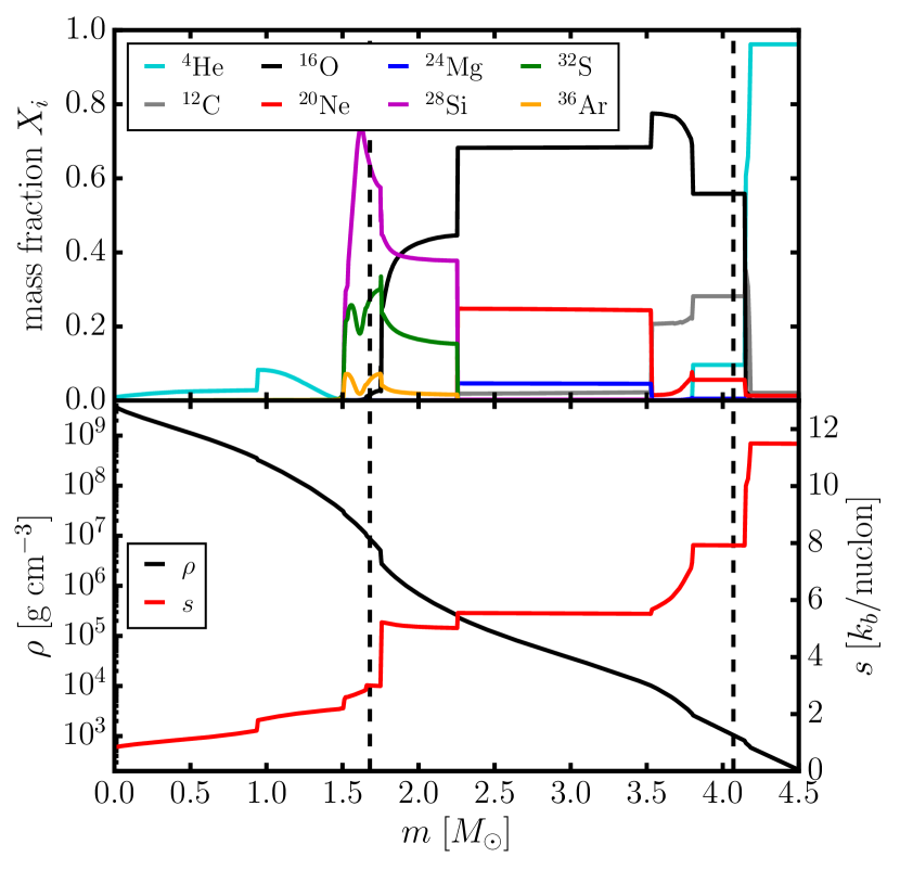
Figure 1.— Top panel: Mass fractions $X_{i}$ of relevant $\alpha$-elements in the 1D progenitor model at the onset of collapse as a function of enclosed mass $m$. Bottom panel: Profiles of entropy $s$ and density $\rho$ as a function of $m$. Dashed vertical lines indicate the boundaries of the region simulated in 3D.

2. Setup and Numerical Methods

2.1. The Kepler Stellar Evolution Code

We simulate oxygen shell burning in a non-rotating $18M_{\odot}$ solar metallicity star. This stellar model has been evolved to the onset of core collapse with an up-to-date version of the stellar evolution code Kepler (Weaver et al., 1978; Woosley et al., 2002; Heger & Woosley, 2010). A 19-species nuclear network (Weaver et al., 1978) is used at low temperatures (up to oxygen burning); at higher temperatures, we switch to a quasi-equilibrium (QSE) approach that provides an efficient and accurate mean to treat silicon burning and the transition to a nuclear statistical equilibrium (NSE) network after silicon depletion.

The mixing processes taken into account in this model include convective mixing according to MLT, thermohaline mixing according to Heger et al. (2005), and semiconvection according to Langer et al. (1983), but modified for a general equation of state as derived in Heger et al. (2005). All mixing is modeled as a diffusive process with appropriately determined diffusion coefficients. Since we will compare the predictions of MLT and the results of our 3D simulation in some detail, we elaborate further on the numerical implementation of MLT in fully convective (Ledoux-unstable) regions in Kepler, which has been outlined in a more compact form in previous papers (Woosley & Weaver, 1988; Woosley et al., 2004). For the implementation of semiconvection and thermohaline convection (which are not immediately relevant for this paper), we refer the reader to Heger et al. (2000, 2005).

MLT assumes that the relative density contrast $\delta\rho/\rho$ between convective updrafts/downdrafts and the spherically averaged background state is related to the deviation of the spherically averaged stratification from convective neutrality and hence to the Brunt-Väisälä frequency $\omega_{\mathrm{BV}}$. If the Ledoux criterion for convection is used (as in Kepler), one obtains

$$\frac{\delta\rho}{\rho}=\Lambda_{\mathrm{mix}}\left(\frac{1}{\rho}\frac{\partial\rho}{\partial r}-\frac{1}{\rho c_{s}^{2}}\frac{\partial P}{\partial r}\right)=\frac{\Lambda_{\mathrm{mix}}\omega_{\mathrm{BV}}^{2}}{g},$$ (1)

for $\delta\rho/\rho$, where both entropy and composition gradients are implicitly taken into account (see Appendix A). Here, $\rho$, $P$, and $c_{s}$ denote the spherically averaged density, pressure, and adiabatic sound speed, and $g$ denotes the local gravitational acceleration. $\omega_{\mathrm{BV}}$ is the Brunt-Väisälä frequency, and $\Lambda_{\mathrm{mix}}$ is the mixing length, which is chosen as one pressure scale height $h_{P}$ so that we have

$$\Lambda_{\mathrm{mix}}=h_{P}=P\left(\frac{\partial P}{\partial r}\right)^{-1}=\frac{P}{\rho g},$$ (2)

under the assumption of hydrostatic equilibrium. The convective velocity in MLT can then be expressed in terms of $\omega_{\mathrm{BV}}$, $\Lambda_{\mathrm{mix}}$, $g$, and $\delta\rho/\rho$, and a dimensionless parameter $\alpha_{1}$ as

$$v_{\mathrm{conv}} = \alpha_{1}\omega_{\mathrm{BV}}\Lambda_{\mathrm{mix}}=\alpha_{1}\left(\frac{\delta\rho}{\rho}\frac{g}{\Lambda_{\mathrm{mix}}}\right)^{1/2}\Lambda_{\mathrm{mix}}$$ (3)

$$= \alpha_{1}\left(g\Lambda_{\mathrm{mix}}\frac{\delta\rho}{\rho}\right)^{1/2}.$$

Note that different normalizations and default values for $\alpha_{1}$ are used in the literature. Wherever a direct calibration against observations (as for the solar convection zone, Christensen-Dalsgaard et al., 1996) is not possible, physical arguments can only constrain $\alpha_{1}$ to within a factor of a few.

Together with the temperature contrast $\delta T$ between the convective blobs and their surroundings, $v_{\mathrm{conv}}$ determines the convective energy flux $F_{\mathrm{conv}}$,

$$F_{\mathrm{conv}} = \alpha_{2}\rho c_{P}\,\delta T\,v_{\mathrm{conv}}=\alpha_{1}\alpha_{2}\rho c_{P}\,\delta T\,\Lambda_{\mathrm{mix}}\omega_{\mathrm{BV}}$$ (4)

$$= -\alpha_{1}\alpha_{2}\rho c_{P}\left(\frac{\partial T}{\partial\ln\rho}\right)_{P}\frac{\delta\rho}{\rho}\Lambda_{\mathrm{mix}}\omega_{\mathrm{BV}}$$

$$= -\alpha_{1}\alpha_{2}\rho c_{P}\left(\frac{\partial T}{\partial\ln\rho}\right)_{P}\frac{\Lambda_{\mathrm{mix}}^{2}\omega_{\mathrm{BV}}^{3}}{g},$$

where $c_{P}$ is the specific heat at constant pressure, and $\alpha_{2}$ is another dimensionless parameter. Note that the second and third line in Equation (4) implicitly assume that the contribution of composition gradients to the unstable gradient can be neglected inside a convective zone, which is a good approximation for advanced burning stages.

For compositional mixing, Kepler uses a time-dependent diffusion model (Eggleton, 1972; Weaver et al., 1978; Heger et al., 2000, 2005) for the evolution of the mass fractions $X_{i}$,

$$\left(\frac{\partial\rho X_{i}}{\partial t}\right)_{\mathrm{mix}}=\frac{1}{r^{2}}\frac{\partial r^{2}F_{X_{i}}}{\partial r}=\frac{1}{r^{2}}\frac{\partial}{\partial r}\left(r^{2}\rho D\frac{\partial X_{i}}{\partial r}\right),$$ (5)

where $F_{X_{i}}=\rho D\partial X_{i}/\partial r$ is the diffusive partial mass flux for species $i$, and the diffusion coefficient is given by

$$D=\alpha_{3}\Lambda_{\mathrm{mix}}v_{\mathrm{conv}}=\alpha_{1}\alpha_{3}\omega_{\mathrm{BV}}\Lambda_{\mathrm{mix}}^{2},$$ (6)

where we have introduced another dimensionless parameter $\alpha_{3}$. If we introduce the composition contrast $\delta X_{i}=\Lambda_{\mathrm{mix}}\partial X_{i}/\partial r$ between the bubbles and the background state, the symmetry to Equation (4) for the convective energy flux becomes manifest:

$$F_{X_{i}}=\alpha_{1}\alpha_{3}\,\rho\,\delta X_{i}\,\Lambda_{\mathrm{mix}}\omega_{\mathrm{BV}}.$$ (7)

We note that only the products $\alpha_{1}\alpha_{2}$ and $\alpha_{1}\alpha_{3}$ enter the evolution equations, and we are therefore free to reshuffle an arbitrary factor between $\alpha_{1}$ and the other two coefficients. In Kepler, we choose $\alpha_{1}\alpha_{2}=1/2$ and $\alpha_{1}\alpha_{3}=1/6$, which is traditionally interpreted as the result of $\alpha_{1}=1/2$, $\alpha_{2}=1$ and $\alpha_{3}=1/3$, where the choice of $\alpha_{3}=1/3$ is motivated by the interpretation of convective mixing as a random-walk process in 3D with mean free path $\Lambda_{\mathrm{mix}}$ and an average total velocity (including the non-radial velocity components) $v_{\mathrm{conv}}$. Setting $\alpha_{3}=\alpha_{2}/3$ arguably introduces an asymmetry in the equations, but we defer the discussion of its effect to Section 3.4. For extracting convective velocities from the Kepler model, we shall work with the alternative choice of $\alpha_{1}=1,\alpha_{2}=1/2,\alpha_{3}=1/6$, however, as this gives better agreement with the convective velocity field in our 3D simulation. This is equally justifiable; essentially this choice amounts to a larger correlation length for velocity perturbations and less perfect correlations between fluctuations in velocity and entropy/composition.

For numerical reasons, $\omega_{\mathrm{BV}}$ is rescaled before computing the convective energy and partial mass fluxes according to Equations (4) and (7),

$$\omega_{\mathrm{BV}}\rightarrow\omega_{\mathrm{BV}}e^{-f/(3\delta\rho/\rho)},$$ (8)

where $f$ is an adjustable parameter that is set to $f=0.01$ in our model. By rescaling $\omega_{\mathrm{BV}}$ convective mixing and energy transport are suppressed until a reasonably large superadiabatic gradient has been established. This procedure avoids convergence problems due to zones switching too frequently between convective stability and instability. The repercussions and limitations of this numerical approach will be discussed in Section 3.1, where we compare the 1D stellar evolution model to our 3D hydrodynamic simulation.

2.2. 1D Supernova Progenitor Model

Entropy, density, and composition profiles of the 1D progenitor model at the onset of collapse are shown in Figure 1. The progenitor has an extended convective oxygen shell of about $0.5M_{\odot}$ with a broader convective carbon burning shell directly on top of it. The inner and outer boundaries of the oxygen shell are located at $3000\,\mathrm{km}$ and $8000\,\mathrm{km}$ at the beginning of our 3D simulation and contract considerably until collapse sets in. The entropy jump between the silicon and oxygen shell is relatively pronounced, so that no strong overshooting and/or entrainment at the inner convective boundary is expected because of the strong buoyancy barrier at the interface. The boundary between the oxygen and carbon shell is considerably “softer” with only a small jump of $0.5\,\mathrm{k}_{b}/\mathrm{nucleon}$ in entropy.

We note that the balance between energy generation by nuclear burning and neutrino cooling is broken during the final phase before collapse that we are considering here. This is due to the acceleration of shell burning induced by the contraction of the core on a time-scale too short for thermal adjustment by neutrino cooling. Different from earlier phases, it is therefore sufficient to follow shell convection in multi-D merely for several overturn time-scales to reach the correct quasi-steady state (instead of several Kelvin-Helmholtz time-scales for earlier phases to ensure thermal adjustment).

2.3. 3D Simulation

At a time of $293.5\,\mathrm{s}$ before the onset of collapse, the stellar evolution model is mapped to the finite-volume hydrodynamics code Prometheus (Fryxell et al., 1989), which is an implementation of the piecewise parabolic method of Colella & Woodward (1984). An axis-free overset “Yin-Yang” grid (Kageyama & Sato, 2004; Wongwathanarat et al., 2010), impelemented as in Melson et al. (2015) using MPI domain decomposition and an algorithm for conservative advection of scalars (Wongwathanarat et al., 2010; Melson, 2013) , allows us to retain the advantages of spherical polar coordinates, which are best suited to the problem geometry, while avoiding excessive time-step constraints close to the grid axis. As in Kepler, nuclear burning is treated using a 19-species $\alpha$-network. The simulations are performed in the so-called implicit large eddy simulations (ILES) paradigm (Boris et al., 1992; Grinstein et al., 2007), in which diffusive processes (viscosity, mass diffusion, thermal diffusion) are not explicitly included in the equations. Instead, one relies on the truncation errors of the underlying numerical scheme to mimic the effects of irreversible processes taking place at unresolved scales (truncation errors act as an “implicit” sub-grid scale model).

Since there is no convective activity in the Fe core and the Si shell in the last stages before collapse in the Kepler model, we excise the innermost $1.68M_{\odot}$ of the core and contract the inner boundary of the computational domain according to the trajectory of this mass shell in the Kepler run from an initial radius of $3000\,\mathrm{km}$ to $1974\,\mathrm{km}$ at the onset of collapse. At both the inner and outer boundary, we impose reflecting boundary conditions for the radial velocity, and use constant extrapolation for the non-radial velocity components. The density, pressure and internal energy are extrapolated into the ghost zones assuming hydrostatic equilibrium and constant entropy. Excising the core not only reduces the computer time requirements considerably, but also allows us to circumvent the complications of deleptonization and Si burning in the QSE regime. The outer boundary is set to a mass coordinate of $4.07M_{\odot}$ (corresponding to a radius of $50,000\,\mathrm{km}$) so that the computational domain comprises the outer $0.08M_{\odot}$ of the Si shell, the entire O and C shell, and a small part of the incompletely burnt He shell. On the other hand, using an inner boundary condition implies that we cannot address potential effects of shell convection on the core via wave excitation at the convective boundaries, such as the excitation of unstable g-mode (Goldreich et al., 1997) (whose growth is likely too slow to be significant; see Murphy et al. 2004) or core spin-up due to angular momentum transport by internal gravity waves (Fuller et al., 2015).

We use a logarithmic radial grid with 400 zones, which implies a radial resolution of $\Delta r/r=0.7\%$ at the beginning of the simulation. Equidistant spacing in $\log r$ is maintained throughout the simulation as the inner boundary is contracted. $56\times 148$ angular zones are used on each patch of the Yin-Yang grid, which corresponds to an angular resolution of $2^{\circ}$. A limited resolution study based on two additional models with coarser meshes is presnted in Appendix B.

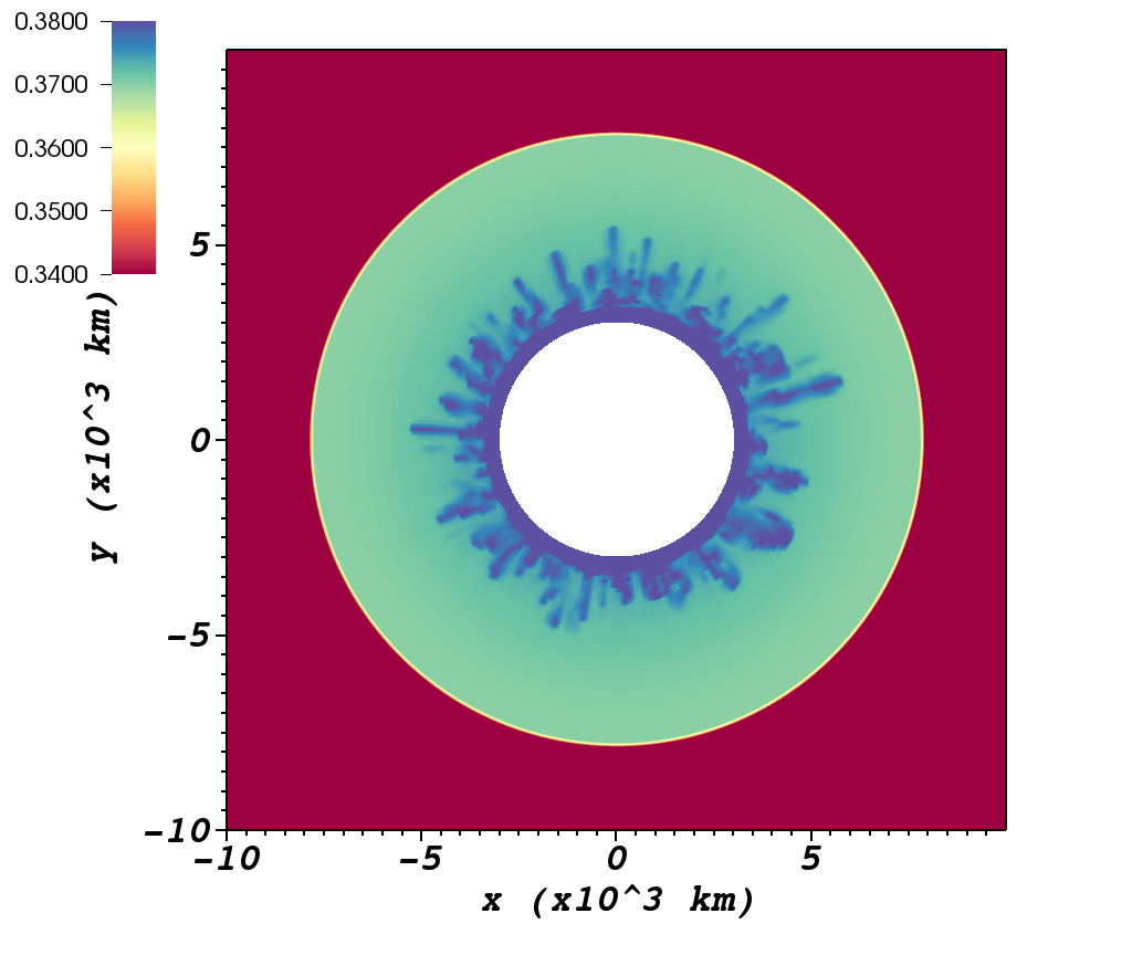
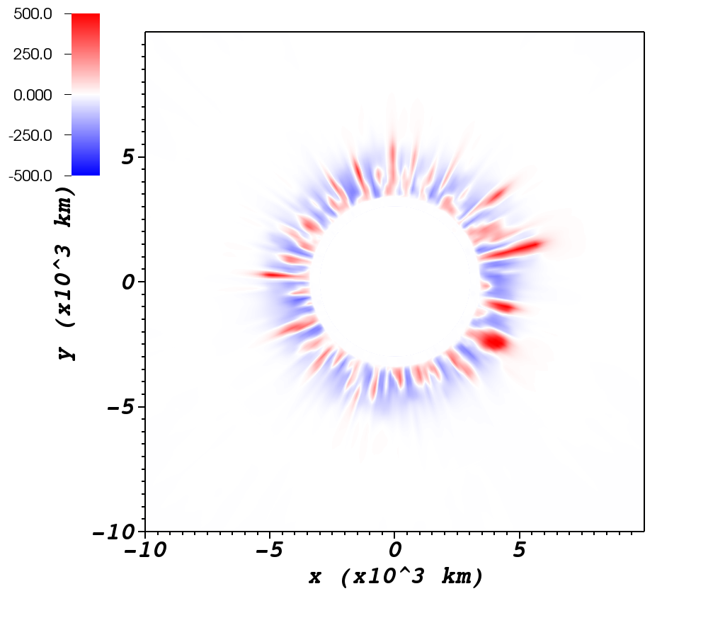
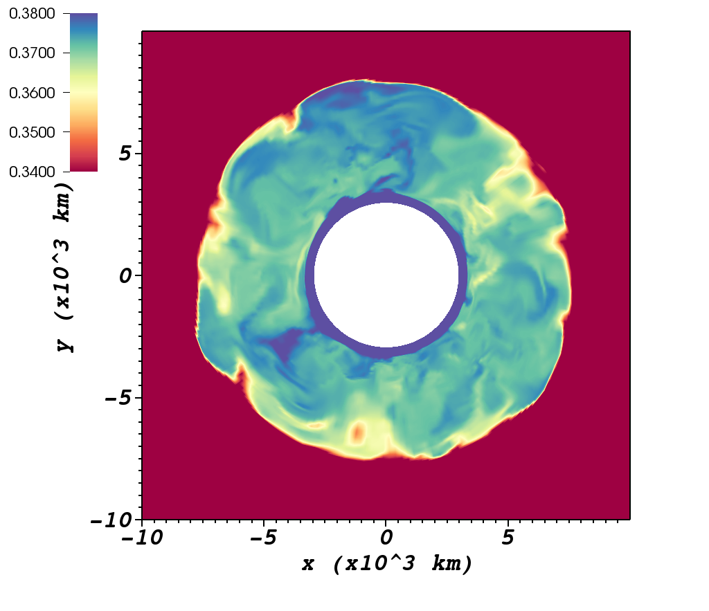
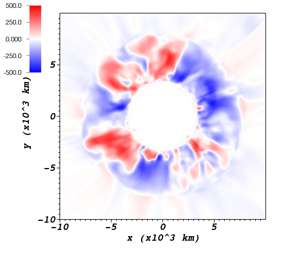
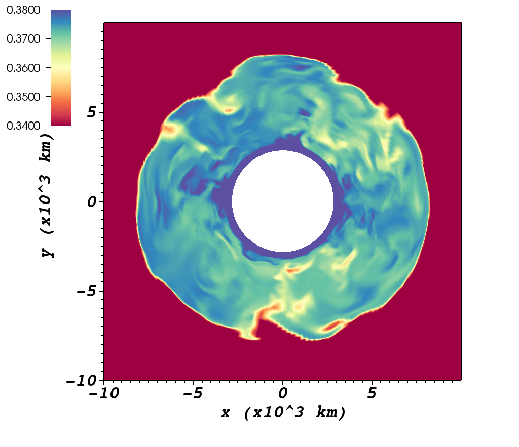
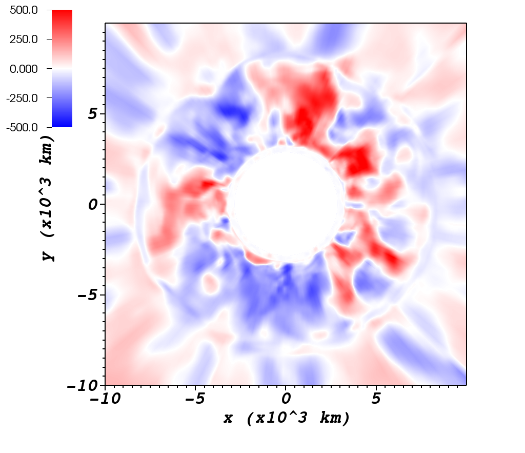
Figure 2.— Slices showing the mass fraction $X_{\mathrm{Si}}$ of silicon (left column) and the radial velocity $v_{r}$ (right column) at times of $20\,\mathrm{s}$, $151\,\mathrm{s}$, and $210\,\mathrm{s}$ after the beginning of the 3D simulation (top to bottom). $v_{r}$ is given in units of $\mathrm{km}\,\mathrm{s}^{-1}$. The boundary between the patches of the Yin-Yang grid is located in the right half of the panels at $45^{\circ}$ and $135^{\circ}$ from the vertical direction. Note that convection initially develops on small angular scales after mapping from the 1D stellar evolution as a strongly superadiabatic gradient builds up in the narrow region of strongest nuclear burning at the base of the oxygen shell (top row). Once convection is fully developed, large-scale overturn emerges. The position of the updrafts and downdrafts shifts freely across the boundaries between the grid patches.

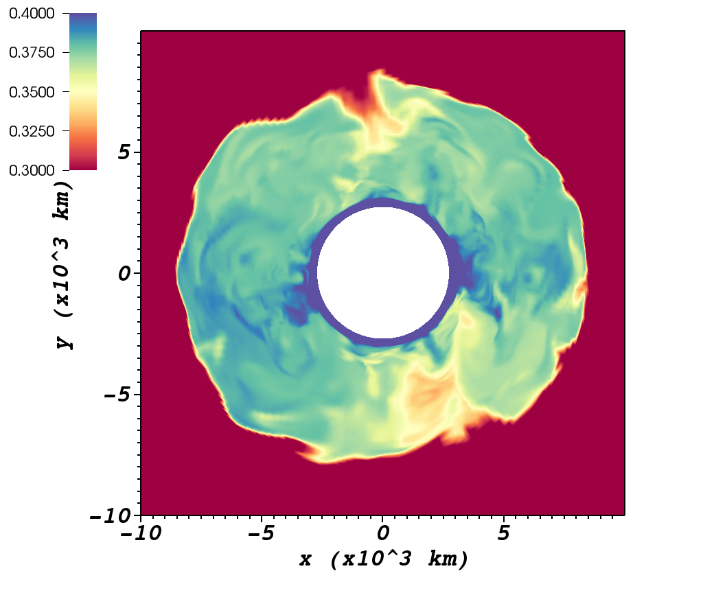
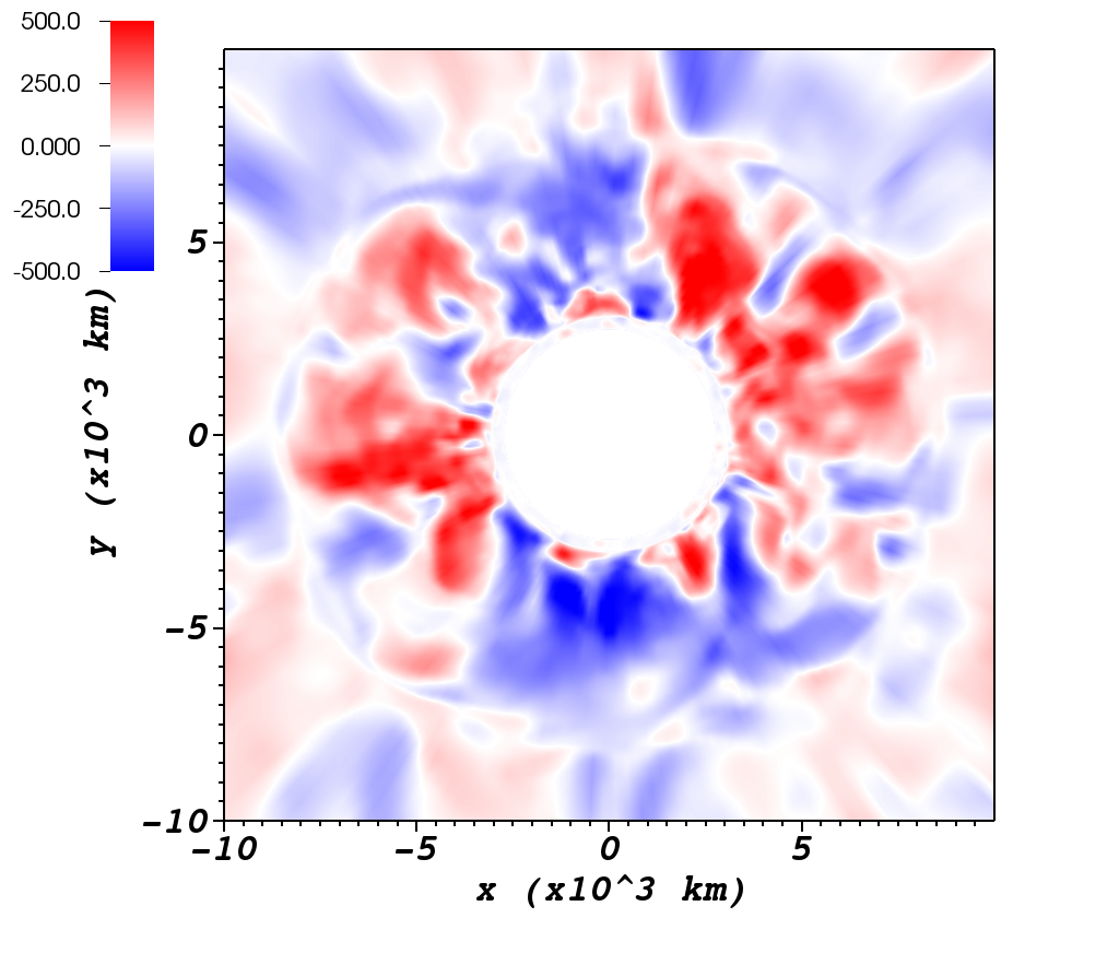
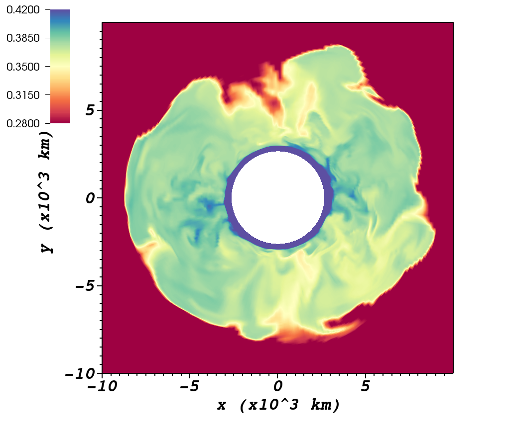
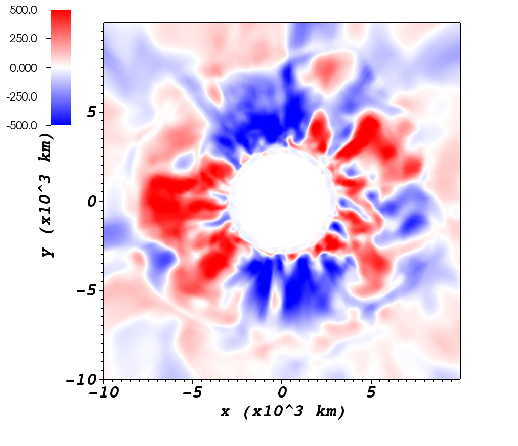
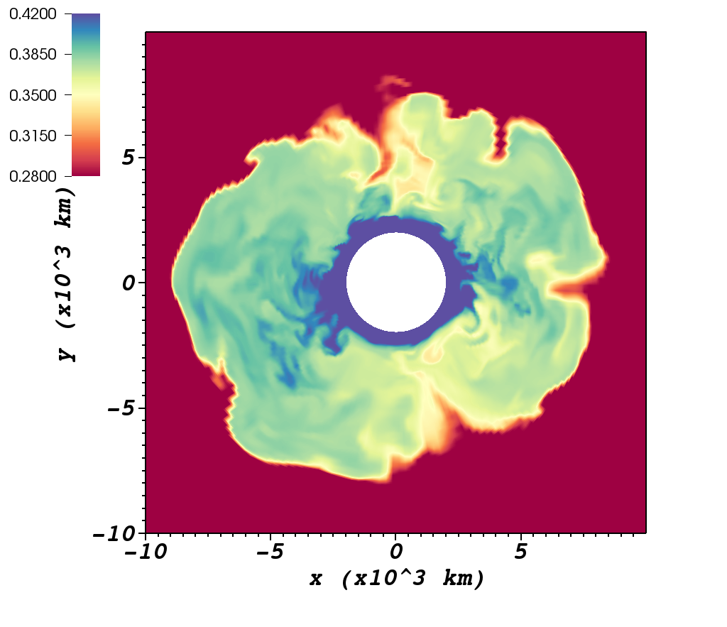
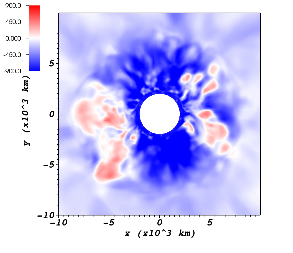
Figure 3.— Slices showing the mass fraction $X_{\mathrm{Si}}$ of silicon (left column) and the radial velocity $v_{r}$ (right column) at times of $270\,\mathrm{s}$, $286\,\mathrm{s}$, and $293.5\,\mathrm{s}$ (onset of collapse) after the beginning of the 3D simulation (top to bottom). $v_{r}$ is given in units of $\mathrm{km}\,\mathrm{s}^{-1}$. Note that wave breaking at the outer boundary of the oxygen shell and the global asymmetry of convective motions become more conspicuous at late times. At the onset of collapse, a bipolar flow pattern emerges (bottom row).

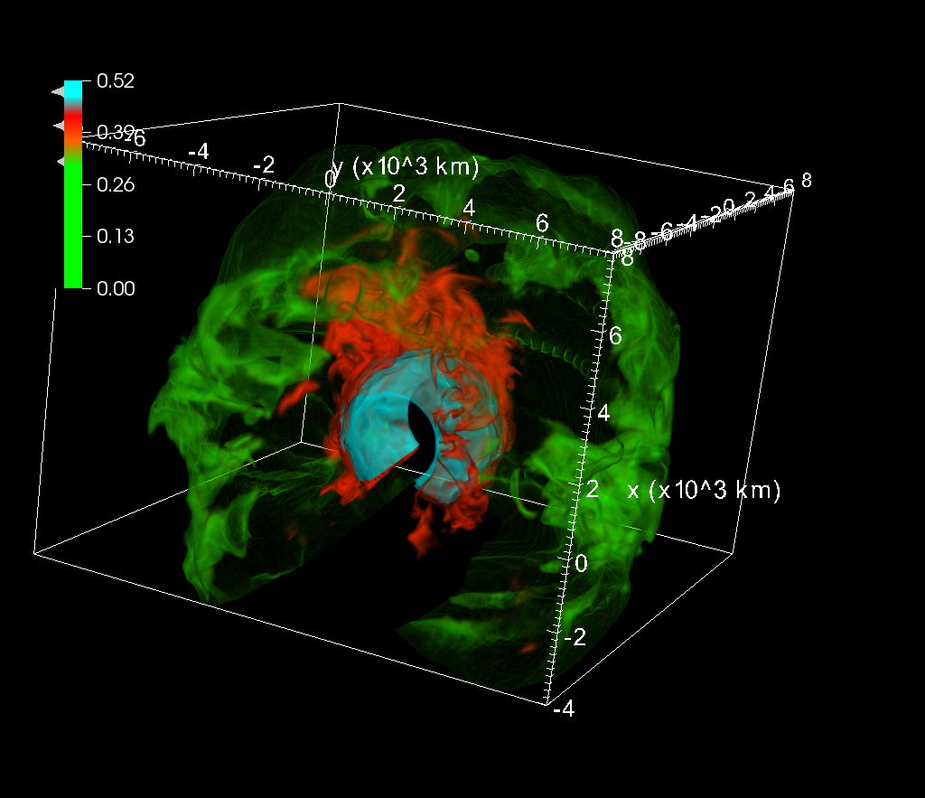
Figure 4.— Volume rendering of the mass fraction of silicon at the end of the 3D simulation at $293.5\,\mathrm{s}$ (onset of collapse) on one patch of the Yin-Yang grid, showing fuzzy silicon-rich updrafts of hot ashes (red) and silicon-poor downdrafts of fresh fuel. A global asymmetry in the updrafts is clearly visible. The inner boundary of the oxygen shell (cyan) is relatively “hard” due to the strong buoyancy jump between the silicon and oxygen shell and therefore remains almost spherical.

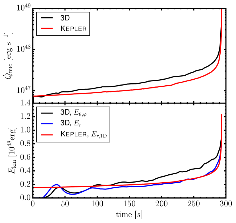
Figure 5.— Top: Volume-integrated net nuclear energy generation rate $\dot{Q}_{\mathrm{nuc}}$ in the oxygen shell in the 3D simulation (black) and in Kepler (red). Bottom: Kinetic energies $E_{\theta,\varphi}$ (black) and $E_{r}$ (blue) contained in fluctuating non-radial and radial motions in the 3D simulation; see Equations (9,10) for definitions. The MLT estimate of the volume-integrated kinetic energy $E_{r,\mathrm{1D}}$ in radial convective motions in the oxygen shell for the Kepler model (red) is computed by using Equation (3) for the convective velocity assuming $\alpha_{1}=1$.

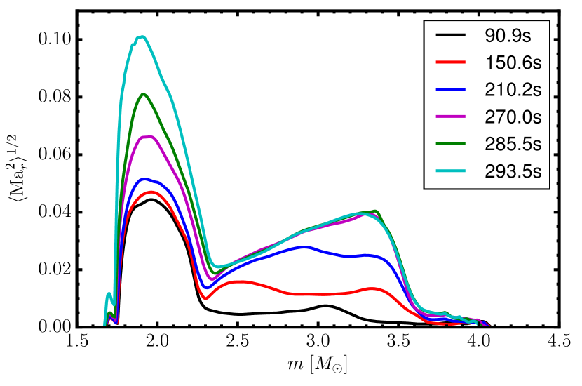
Figure 6.— Profiles of the turbulent Mach number $\sqrt{\langle\mathrm{Ma}_{r}^{2}\rangle}$ of radial velocity fluctuations in the oxygen and carbon shell at different times during the 3D simulation. Note that there is a secular increase in the Mach number in the oxygen shell even after convection has reached a quasi-stationary state due to the contraction of the inner boundary. By contrast, the turbulent Mach number in the carbon shell merely increases because convection has not reached a quasi-stationary state in that shell.

Figure 7.— Top panel: Efficiency $\eta_{\mathrm{conv}}$ for the conversion of nuclear energy generation into convective kinetic energy as defined in Equation (14) in the 3D run and the 1D Kepler model. In the 3D case, we compute $\eta_{\mathrm{conv}}$ both for the kinetic energy in radial motions (Equation 9, black curve) and transverse motions (Equation 10, blue); for the Kepler run (red), we use the energy contained in radial convective motions computed according to Equation (13). By default, we use the pressure scale height in Equation (14) as the mixing or damping length $\Lambda_{\mathrm{damp}}$. The efficiency is much lower if $\Lambda_{\mathrm{damp}}$ is identified with the radial extent of the convective zone $\Lambda_{\mathrm{conv}}=r_{+}-r_{-}$. Bottom panel: Comparison of the Brunt-Väisälä frequency $\omega_{\mathrm{BV,max}}$ at the base of the oxygen shell (black), the reciprocal of the convective turnover time $t_{\mathrm{conv}}$ (blue), and the logarithmic derivative $\mathrm{d}\ln\dot{Q}_{\mathrm{nuc}}/\mathrm{d}t$ of the volume-integrated nuclear energy generation rate (red). The freeze-out of convection (denoted by a dashed vertical line) occurs roughly when $\omega_{\mathrm{BV,max}}/(2\pi)\approx t_{\mathrm{conv}}^{-1}\approx\mathrm{d}\ln\dot{Q}_{\mathrm{nuc}}/\mathrm{d}t$.

3. Simulation Results

In Figures 2 and 3, we show 2D slices depicting the evolution of the mass fraction $X_{\mathrm{Si}}$ of silicon and the radial velocity $v_{r}$ to provide a rough impression of the multi-D flow dynamics in our 3D simulation. Convective plumes initially develop on small angular scales in the inner part of the oxygen shell (where the burning rate is high). After about $100\,\mathrm{s}$ we see fully developed convection with maximum plume velocities of $\mathord{\sim}500\,\mathrm{km}\,\mathrm{s}^{-1}$ that increase towards collapse, and large-scale modes dominate the flow. The latest snapshots at $286\,\mathrm{s}$ and $293.5\,\mathrm{s}$ suggest the emergence of a bipolar flow structure right before collapse. Large-scale structures are more clearly visible in the velocity field than in $X_{\mathrm{Si}}$. Indeed, the rising plumes enriched in silicon and the sinking plumes containing fresh fuel appear rather “wispy”, an impression which is reinforced by the 3D volume rendering of $X_{\mathrm{Si}}$ at the onset of collapse in Figure 4.

Convection also develops in the overlying carbon shell. However, since the convective velocities in the carbon shell are lower, and since this shell extends out to a radius of $27,000\,\mathrm{km}$, convection never reaches a quasi-steady state within the simulation time. We therefore do not address convection in the carbon shell in our analysis.

As in earlier studies of mixing at convective boundaries (Meakin & Arnett, 2007b), the interface between the carbon and oxygen layer proves unstable to the Holmböe/Kelvin-Helmholtz instability with wave breaking leading to the entrainment of material from the carbon shell. The snapshots suggest that such entrainment events become more frequent and violent shortly before collapse.

The convective velocities and eddy scales thus fall roughly into the regime where the parametric study of Müller & Janka (2015) suggests a significant impact of pre-collapse asphericities on shock revival (a convective Mach number of order $0.05$ or higher, corresponding to velocities of a few $100\,\mathrm{km}\,\mathrm{s}^{-1}$, and dominant $\ell=1$ or $\ell=2$ modes).

Figure 8.— Top: Outer and inner boundary radius $r_{+}$ and $r_{-}$ of the oxygen shell as functiosn of time. Bottom: Correlation length $\Lambda_{\mathrm{corr}}$ for the radial velocity computed at $r=4000\,\mathrm{km}$ (black), pressure scale height $h_{P}$ at the base of the oxygen shell (red) and radial extent $\Lambda_{\mathrm{conv}}=r_{+}-r_{-}$ of the oxygen shell (blue) as a function of time.

Figure 9.— Top: Total convective luminosity (including the kinetic energy flux) at $210\,\mathrm{ms}$ in the 3D simulation as a function of enclosed mass $m$. Bottom: Quantities determining the spherically averaged entropy production. The term $T^{-1}\mathrm{d}L_{\mathrm{conv}}/\mathrm{d}m$ stemming from the divergence of the total convective luminosity is shown in red, the entropy production due to the nuclear source term $\dot{\epsilon}_{\mathrm{nuc}}/T$ (neglecting terms in the chemical potential of the different nuclear species) is shown in blue, and the black curve denotes the sum of both terms. The curves are computed from averages over several time steps.

Figure 10.— Top panel: comparison of radial and transverse RMS velocity fluctuations $\delta v_{r}$ (black) and $\delta v_{t}$ (blue) in the 3D model at $210\,\mathrm{s}$ to the convective velocity $v_{\mathrm{conv}}$ computed in the Kepler model using MLT (red), and to $\omega_{\mathrm{BV}}h_{P}$ (violet). Bottom panel: Comparison of the Brunt-Väisälä frequency computed from spherical averages of the pressure, density, and sound speed in the 3D run (black) and in the 1D Kepler model. Note that there is a formally stable region around the boundary between the oxygen and carbon shell in the 3D model due to the aspherical deformation of the shell boundary and the entrainment of material from the carbon shell, which increases the spherically averaged entropy in the outer parts of the oxygen shell.

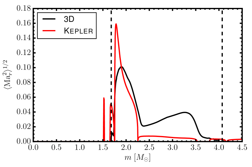
Figure 11.— Profiles of the RMS-averaged turbulent Mach number $\langle\mathrm{Ma}_{r}^{2}\rangle^{1/2}$ of radial velocity fluctuations at the onset of collapse in the 3D model (black) and the 1D Kepler model (red). Dashed lines denote the boundaries of the domain simulated in 3D in Prometheus. The turbulent Mach number in 1D and 3D agrees well in the bulk of the oxygen shell, but the acceleration of nuclear burning and the concomitant increase of the Brunt-Väisälä frequency artificially increases the convective velocities close to the base of the shell in Kepler, as MLT immediately translates the increase in $\omega_{\mathrm{BV}}$ into an increase in convective velocity. Note that high nuclear burning rates in individual zones inside the silicon core produce formally unstable zones in the Kepler run shortly before collapse, which do not affect the evolution of the model to any significant degree.

3.1. Flow Dynamics for Quasi-Stationary Convection– Quantitative Analysis and Comparison with MLT

To analyze the flow dynamics more quantitatively, we consider the volume-integrated net nuclear energy generation rate (including neutrino losses) in the oxygen shell, $\dot{Q}_{\mathrm{nuc}}$, the volume-integrated turbulent kinetic energy $E_{r}$ and $E_{\theta,\varphi}$ contained in the fluctuating components of radial and non-radial velocity components, and profiles of the root-mean-square (RMS) averaged turbulent Mach number $\langle\mathrm{Ma}_{r}^{2}\rangle^{1/2}$ of the radial velocity fluctuations in Figures 5 and 6. $E_{r}$, $E_{\theta,\varphi}$, and $\langle\mathrm{Ma}^{2}\rangle^{1/2}$, are computed from the velocity field as follows,

$$E_{r} = \frac{1}{2}\int\limits_{r_{-}\leq r\leq r_{+}}\rho(v_{r}-\langle v_{r}\rangle)^{2}\,\mathrm{d}V,$$ (9)

$$E_{\theta,\varphi} = \frac{1}{2}\int\limits_{r_{-}\leq r\leq r_{+}}\rho(v_{\theta}^{2}+v_{\varphi}^{2})\,\mathrm{d}V,$$ (10)

$$\langle\mathrm{Ma}_{r}^{2}\rangle^{1/2} = \left[\frac{\int\rho(v_{r}-\langle v_{r}\rangle)^{2}\,\mathrm{d}\Omega}{\int\rho c_{s}^{2}\,\mathrm{d}\Omega}\right]^{1/2},$$ (11)

where the domain of integration in Equations (9) and (10) extends from the inner boundary radius $r_{-}$ to the outer boundary radius $r_{+}$ of the oxygen shell. Angled brackets denote mass-weighted spherical Favre averages for quantity $X$,

$$\langle X\rangle=\frac{\int\rho X\,\mathrm{d}\Omega}{\int\rho\,\mathrm{d}\Omega}.$$ (12)

We note that one does not expect any mean flow in the non-radial directions in the absence of rotation; therefore only $v_{\theta}$ and $v_{\varphi}$ appear in Equation (10). In Figure 5, we also show the results for $\dot{Q}_{\mathrm{nuc}}$ and the kinetic energy in convective motions from the 1D Kepler run for comparison. MLT only predicts the radial velocities of rising and sinking convective plumes, so we only compute the 1D analog to $E_{r}$,

$$E_{r,\mathrm{1D}}=\frac{1}{2}\int\limits_{r_{-}}^{r_{+}}\rho v_{\mathrm{conv}}^{2}\,\mathrm{d}V,$$ (13)

where $v_{\mathrm{conv}}$ is calculated according to Equation (3).

The volume-integrated nuclear energy generation rate $\dot{Q}_{\mathrm{nuc}}$ increases by more than two orders of magnitude during the evolution towards collapse. Due to slight structural adjustments after the initial transient and slightly different mixing in the 3D model, $\dot{Q}_{\mathrm{nuc}}$ is roughly $30\ldots 50\%$ higher in 3D than in the Kepler for most of the run (see discussion in Section 3.4), but still parallels the Kepler run quite nicely and perhaps as closely as can be expected given the extreme dependence of the local energy generation $\dot{\epsilon}_{\mathrm{nuc}}\propto T^{30}$ on the temperature $T$ during oxygen burning.

The convective kinetic energy oscillates considerably during the first $120\,\mathrm{s}$, but exhibits a smooth secular increase reflecting the acceleration of nuclear burning. Equipartition between the radial and non-radial kinetic energy in convective motions as suggested by Arnett et al. (2009) does not hold exactly, instead we observe $E_{\mathrm{\theta,\varphi}}>E_{r}$ for most of the simulation, suggesting that there may not be a universal ratio between the non-radial and radial kinetic energy and that this ratio is instead somewhat dependent on the shell geometry (width-to-radius ratio, ratio of width and pressure scale height), which can vary across different burning shells, progenitors, and evolutionary phases. There may also be stochastic variations in the eddy geometry that the convective flow selects (see Appendix B) . Anisotropic numerical dissipation might also account for different results in different numerical simulations. The turbulent Mach number in the oxygen shell (Figure 6) also increases steadily from about $0.04\ldots 0.05$ after the initial transient to $0.1$ at collapse.

Again, there is reasonable agreement between the MLT prediction $E_{r,\mathrm{1D}}$ for the convective kinetic energy and $E_{r}$ in the 3D simulation (Figure 5). $E_{r,\mathrm{1D}}$ and $E_{r}$ are in fact closer to each other than $E_{\mathrm{\theta,\varphi}}$ and $E_{r}$ in 3D. Somewhat larger deviations arise immediately prior to collapse when convection is no longer fast enough to adjust to the acceleration of nuclear burning as we shall discuss in Section 3.2.

Except for the last few seconds, the kinetic energy in convection scales nicely with the nuclear energy generation rate both in 1D and 3D. For a case where the convective luminosity $L_{\mathrm{conv}}$ and $\dot{Q}_{\mathrm{nuc}}$ balance each other in the case of steady-state convection, MLT implies $v_{\mathrm{conv}}^{3}\sim\dot{Q}_{\mathrm{nuc}}\Lambda_{\mathrm{mix}}/M_{\mathrm{conv}}$, where $M_{\mathrm{conv}}$ is the mass contained in the convective shell (Biermann, 1932; Arnett et al., 2009, note that only the form of the equations is slightly different in these references). In Figure 7, we show the efficiency factors $\eta_{\mathrm{conv}}$ for the conversion of nuclear energy generation into turbulent kinetic energy $E_{\mathrm{turb}}$,

$$\eta_{\mathrm{conv}}=\frac{E_{\mathrm{turb}}/M_{\mathrm{conv}}}{(\dot{Q}_{\mathrm{nuc}}\Lambda_{\mathrm{mix}}/M_{\mathrm{conv}})^{2/3}},$$ (14)

for both the 3D model (using either the component $E_{r}$ or $E_{\theta,\varphi}$ for $E_{\mathrm{turb}}$) and the Kepler model (using $E_{\mathrm{turb}}=E_{r,\mathrm{1D}}$), with $\Lambda_{\mathrm{mix}}$ set to the pressure scale height at the inner boundary of the oxygen shell. Between $130\,\mathrm{s}$ and $290\,\mathrm{s}$, $\eta_{\mathrm{conv}}$ shows only small fluctuations around $0.35$ and $0.5$ for the kinetic energy in radial and non-radial convective motions in 3D. For the Kepler model, we find similar values around $\eta_{\mathrm{conv}}\approx 0.37$.

The scaling law $v_{\mathrm{conv}}^{3}\sim\dot{Q}_{\mathrm{nuc}}\Lambda_{\mathrm{mix}}/M_{\mathrm{conv}}$ can also be understood as resulting from a balance of buoyant driving (or, equivalently, kinetic energy generation by a heat engine) and turbulent dissipation (see, e.g.  Arnett et al. 2009 and in a different context Müller & Janka 2015). In this picture, the scaling law emerges if the mixing length is identified with the damping length $\Lambda_{\mathrm{damp}}$. This identification ($\Lambda_{\mathrm{damp}}=\Lambda_{\mathrm{mix}}=h_{P}$), however, has been criticized on the ground that $\Lambda_{\mathrm{damp}}$ should correspond to the largest eddy scale, which can be considerably larger than $h_{P}$ if low-$\ell$ modes dominate the flow and the updrafts and downdrafts traverse the entire convection zone, which is precisely the situation that is realized in our 3D model. The disparity of the pressure scale height and the eddy scale can be quantified more rigorously by considering the radial correlation length $\Lambda_{\mathrm{corr}}$ for fluctuations in the radial velocity, $v^{\prime}_{r}=v_{r}-\langle v_{r}\rangle$. Following Meakin & Arnett (2007b) and Viallet et al. (2013) we compute the vertical correlation length $\Lambda_{\mathrm{corr}}$ as the full width at half maximum of the correlation function $C(r,\delta r)$,

$$C(r,\delta r)=\frac{\langle v_{r}^{\prime}(r,\theta,\varphi)v_{r}^{\prime}(r+\delta r,\theta,\varphi)\rangle}{\sqrt{\langle{v^{\prime}}_{r}^{2}(r,\theta,\varphi)\rangle\langle{v^{\prime}}_{r}^{2}(r+\delta r,\theta,\varphi)\rangle}}.$$ (15)

The correlation function is computed at a radius of $r=4000\,\mathrm{km}$ in the inner half of the oxygen shell. $\Lambda_{\mathrm{corr}}$ is shown in Figure 8 and compared to the pressure scale height $\Lambda_{\mathrm{mix}}=h_{P}$ at the inner boundary of the oxygen shell and the extent $\Lambda_{\mathrm{conv}}$ of the convective region. Once convection is fully developed, we clearly have $\Lambda_{\mathrm{corr}}>\Lambda_{\mathrm{mix}}$ and $\Lambda_{\mathrm{corr}}\approx\Lambda_{\mathrm{conv}}/2$ (as expected for updrafts and downdrafts reaching over the entire zone).

Arnett et al. (2009) argued that the damping length should be of the order of the width $\Lambda_{\mathrm{conv}}$ of the convective zone under such circumstance. If we compute the efficiency factor $\eta_{\mathrm{conv}}$ based on $\Lambda_{\mathrm{conv}}$,

$$\eta_{\mathrm{conv}}=\frac{E_{\mathrm{turb}}/M_{\mathrm{conv}}}{(\dot{Q}_{\mathrm{nuc}}\Lambda_{\mathrm{conv}}/M_{\mathrm{conv}})^{2/3}},$$ (16)

we obtain suspiciously low values $\eta_{\mathrm{conv}}\lesssim 0.1$, however. This suggests that the effective damping length is set by the pressure scale height (or a multiple thereof) after all. One could opine that the energetics of the flow might still be described adequately by $\Lambda_{\mathrm{damp}}=\Lambda_{\mathrm{corr}}$, and that the efficiency factor $\eta_{\mathrm{conv}}$ merely happens to be relatively low.

We argue, however, that there is a deeper reason for identifying $\Lambda_{\mathrm{damp}}$ with a multiple of the pressure scale height in the final phases of shell convection when neutrino cooling can no longer balance nuclear energy generation. The crucial point is that the average distance after which buoyant convective blobs have to return their excess enthalpy $h^{\prime}$ to their surroundings cannot become arbitrarily large in a steady-state situation, and since enthalpy and velocity fluctuations $v^{\prime}$ are correlated ($h^{\prime}\sim v^{\prime 2}$), this also limits the damping length.

During the final stages, nuclear energy generation, convective transport, and turbulent dissipation must balance each other in such a way as to avoid both a secular build-up of an ever-growing unstable entropy/composition gradient (although the spherically average stratification always remains slightly unstable) and a complete erasure of the superadiabatic gradient. Assuming that the Brunt-Väisälä frequency is primarily set by the gradient of the entropy $s$, this implies $\partial^{2}s/\partial r\partial t\approx 0$, and hence roughly constant entropy generation,

$$\dot{s}=\frac{\partial s}{\partial t}\approx\mathrm{const.}$$ (17)

throughout the convective region. In the late pre-collapse stages, we can relate $\dot{s}$ to the local nuclear energy generation rate $\dot{\epsilon}_{\mathrm{nuc}}$ and the derivative of the “total” convective luminosity $L_{\mathrm{conv}}$,

$$\dot{s}\approx\frac{\dot{\epsilon}_{\mathrm{nuc}}}{T}+\frac{1}{T}\frac{\partial L_{\mathrm{conv}}}{\partial m}=\frac{\dot{\epsilon}_{\mathrm{nuc}}}{T}+\frac{1}{4\pi r^{2}\rho T}\frac{\partial L_{\mathrm{conv}}}{\partial r}.$$ (18)

Here, $L_{\mathrm{conv}}$ denotes the net total energy flux resulting from fluctuations (denoted by primes) in the total energy density and velocity around their spherical Favre average,

$$L_{\mathrm{conv}}=r^{2}\int\left[\rho e+P+\rho\frac{v^{2}}{2}\right]^{\prime}v^{\prime}_{r}\,\mathrm{d}\Omega,$$ (19)

where $e$ is the specific internal energy, and $P$ the pressure. Note that in formulating Equation (18), we implicitly assumed that $\partial{L_{\mathrm{conv}}}/\partial m$ is equal to the rate of change of the Favre average of the internal energy $e$ (instead of the total energy density, which includes the contribution of the turbulent kinetic energy). This assumption is justified for steady-state convection in the late pre-collapse phase because of moderate Mach numbers and the minor role of neutrino cooling. These two factors imply that the energy that is generated by nuclear reactions and distributed throughout the unstable region by convection mostly goes into internal energy (whereas our argument cannot be applied to earlier phases where neutrino cooling and nuclear energy generation balance each other).

Figure 9 shows the two terms contributing to $\dot{s}$ in Equation (18) based on Favre averages over a few time steps around $210\,\mathrm{s}$, and demonstrates that $\dot{s}$ is indeed roughly constant throughout the convective region. Since strong nuclear burning is confined to a narrow layer at the bottom of the convective shell, we even have $T^{-1}\partial L_{\mathrm{conv}}/\partial m\approx\mathrm{const.}$ throughout a large part of the shell, and for a stratification with roughly $\rho\propto r^{-3}$ and $T\propto r^{-1}$, this leads to

$$\frac{\partial L_{\mathrm{conv}}}{\partial r}\propto r^{2}\rho T\propto r^{-2}.$$ (20)

For such an idealized case, one can directly compute that the energy transported by convective blobs from the lower boundary must be dissipated after an average distance of

$$\Lambda_{\mathrm{damp}} = -\frac{1}{L_{\mathrm{conv}}(r_{-})-L_{\mathrm{conv}}(r_{+})}\int\limits_{r_{-}}^{r_{+}}(r-r_{-})\frac{\partial L_{\mathrm{conv}}}{\partial r}\mathrm{d}r$$ (21)

$$= r_{-}\left(\frac{\xi\ln\xi}{\xi-1}-1\right),$$

where $\xi=r_{+}/r_{-}$ is the ratio of the outer and inner boundary radius. Evidently, $\Lambda_{\mathrm{damp}}$ grows only moderately at large $\xi$, and is always smaller than $(r_{+}-r_{-})/2$.

It thus appears unlikely that large damping lengths $\Lambda_{\mathrm{damp}}\approx r_{+}-r_{-}\gg h_{P}$ can be realized in very extended convection zones in the final pre-collapse stage. This is decidedly different to earlier stages with strong neutrino cooling in the outer part of the convective zone, for which Arnett et al. (2009) found high values of $\Lambda_{\mathrm{damp}}=0.85(r_{+}-r_{-})$. As outlined before, the different behavior is likely due to the specific physical conditions right before collapse; in the absence of strong cooling, the self-regulatory mechanism that we outlined above automatically ensures that $\Lambda_{\mathrm{damp}}$ cannot be considerably larger than the pressure scale height. Thus, the implicit identification of $\Lambda_{\mathrm{damp}}$ and $h_{P}$ (or a multiple thereof) in MLT is likely less critical for shell convection right before collapse than for earlier phases.

However, it still remains to be determined whether the damping length can reach considerably higher values in deep convection zones with $\xi\gg 1$ during earlier stages when nuclear energy generation and neutrino cooling balance each other. Since neutrino cooling generally decreases with radius within a shell, it can still be argued that the convective luminosity must decay not too far away from the burning region. Thus, an analog to Equation (21) could still hold, and the damping length would only increase slowly with the width of the shell in the limit of large $\xi$. In that case, the difference between our simulation and the results of Arnett et al. (2009) would merely be due to a different depth of the convective zone, which is much deeper in our model ($4\ldots 5$ pressure scale heights as opposed to $\mathord{\sim}2$ pressure scale heights in Arnett et al. 2009) so that we approach a “saturation limit” for the damping length and can more conveniently distinguish the damping length from the width of the convective zone since the different length scale are sufficiently dissimilar.

Radial profiles of the convective velocities also point to reasonable agreement between MLT and the 3D simulation. In the upper panel of Figure 10, we compare the convective velocities from Kepler to RMS averages of the fluctuations of the radial velocity ($\delta v_{r}$) and the transverse velocity component ($\delta v_{t}$) at $210\,\mathrm{s}$,

$$\delta v_{r} = \left(\frac{\int\rho(v_{r}-\langle v_{r}\rangle)^{2}\,\mathrm{d}\Omega}{\int\rho\,\mathrm{d}\Omega}\right)^{1/2},$$ (22)

$$\delta v_{t} = \left(\frac{\int\rho(v_{\theta}^{2}+v_{\varphi}^{2})\,\mathrm{d}\Omega}{\int\rho\,\mathrm{d}\Omega}\right)^{1/2}.$$ (23)

We also compare these to the MLT estimate $v_{\mathrm{conv}}=\omega_{\mathrm{BV}}\Lambda_{\mathrm{mix}}$ computed from the Brunt-Väisälä frequency for the spherically averaged stratification of the 3D model. It is evident that the agreement especially between $\delta v_{r}$ and the convective velocity in Kepler is very good in the oxygen shell. In large parts of the shell, $v_{\mathrm{conv}}=\omega_{\mathrm{BV}}\Lambda_{\mathrm{mix}}$ is also in very good agreement with $\delta v_{r}$, which again demonstrates that the choice of the pressure scale height as the acceleration and damping length for convective blobs is a reasonable choice. However, no reasonable comparison can be made in the outer part of the oxygen shell, where $\omega_{\mathrm{BV}}$ is formally negative. This is due to the strong aspherical deformation of the shell boundary and the entrainment of light, buoyant material from the carbon shell; the fact that the outer part of the oxygen shell is formally stable if $\omega_{\mathrm{BV}}$ is computed from spherical averages of the density and pressure is thus merely a boundary effect and has no bearing on the validity of MLT in the interior of the shell.

The good agreement between the 3D simulation and the Kepler model may seem all the more astonishing considering the rescaling of the Brunt-Väisälä frequency according to Equation (8) for stability reasons. However, this procedure is justified by the fact that the convective luminosity automatically adjusts itself in such a way as to avoid a secular build-up of $\omega_{\mathrm{BV}}$ as discussed before. In a steady state, the convective luminosity in MLT in a shell will roughly balance the nuclear energy generation rate, $L_{\mathrm{conv}}=4\pi r^{2}F_{\mathrm{conv}}\sim\dot{Q}_{\mathrm{nuc}}$, regardless of whether $\omega_{\mathrm{BV}}$ is rescaled or not. If a rescaling factor is introduced in Equation (4), the result is simply that a larger $\omega_{\mathrm{BV}}$ is maintained under steady state conditions to balance the rescaling factor. Except for pathological situations, the convective energy flux and the convective velocities are thus essentially unaffected by this procedure. The superadiabaticity of the stratification is changed, however. For convection at low Mach number, it will be systematically overestimated. This trend is evident from the lower panel of Figure 10, which compares $\omega_{\mathrm{BV}}$ in Kepler and the 3D simulation. Since convection is not extremely subsonic in our case, the rescaling factor is only slightly smaller than unity, and the superadiabaticity in the 1D and 3D model remains quite similar.

3.2. Freeze-Out of Convection

MLT in Kepler thus provides good estimates for the typical convective velocities in the final stages of oxygen shell burning as long as a steady-state balance between nuclear energy generation, convective energy transport, and turbulent dissipation is maintained. However, steady-state conditions are not maintained up to collapse. Figure 7 shows that the growth of the turbulent kinetic energy can no longer keep pace with the acceleration of nuclear burning in the last few seconds before collapse, where $\eta_{\mathrm{conv}}$ drops dramatically.

The time at which convection “freezes out” can be nicely determined by appealing to a time-scale argument: Freeze-out is expected once the nuclear energy generation rate (which sets the Brunt-Väisälä frequency and the convective velocity under steady-state conditions) changes significantly over a turnover time-scale. More quantitatively, the efficiency factor $\eta_{\mathrm{conv}}$ drops abruptly once the freeze-out condition

$$\frac{1}{\dot{Q}_{\mathrm{nuc}}}\frac{\mathrm{d}\dot{Q}_{\mathrm{nuc}}}{\mathrm{d}t}=\frac{\omega_{\mathrm{BV,max}}}{2\pi}$$ (24)

is met as shown in the bottom panel of Figure 7. Equivalently, the freeze-out condition can be expressed in terms of the convective turnover time $t_{\mathrm{conv}}$,

$$t_{\mathrm{conv}}=\frac{\Lambda_{\mathrm{conv}}}{\bar{v}_{\mathrm{conv}}},$$ (25)

where $\bar{v}_{\mathrm{conv}}$ is an appropriate global average of the convective velocity, e.g.,

$$\bar{v}_{\mathrm{conv}}=(2E_{\mathrm{kin},r}/M_{\mathrm{conv}})^{1/2}.$$ (26)

Using these definitions, we find that freeze-out occurs roughly when

$$\frac{1}{\dot{Q}_{\mathrm{nuc}}}\frac{\mathrm{d}\dot{Q}_{\mathrm{nuc}}}{\mathrm{d}t}=t_{\mathrm{conv}}^{-1},$$ (27)

which may be even more intuitive than Equation (24)

Somewhat astonishingly, the Kepler run shows a similar drop of $\eta_{\mathrm{conv}}$ in the last seconds, although MLT implicitly assumes steady-state conditions when estimating the density contrast and the convective velocity. Kepler still overestimates the volume-integrated turbulent kinetic energy somewhat after freeze-out (Figure 5), but the discrepancy between the 1D and 3D models is not inordinate.

The key to the relatively moderate differences can be found in profiles of the turbulent convective Mach number $v_{\mathrm{conv}}/c_{s}$ in Kepler and $\langle\mathrm{Ma}_{r}^{2}\rangle^{1/2}$ in 3D at the onset of collapse in Figure 11. Evidently, MLT only overestimates the convective velocities in a narrow layer at the lower boundary of the oxygen shell, where the acceleration of nuclear burning greatly amplifies the superadiabaticity of the stratification (as quantified by $\omega_{\mathrm{BV}}$). This immediately increases $v_{\mathrm{conv}}$, whereas the convective velocity field adjusts only on a longer time-scale ($\mathord{\gtrsim}\omega_{\mathrm{BV}}^{-1}$) in 3D. However, even in the Kepler run, the convective velocities in the middle and outer region of the oxygen shell remain unaffected by the increase of the $\omega_{\mathrm{BV}}$ close to the inner shell boundary. Different from the innermost region, where $\omega_{\mathrm{BV}}$ reacts instantaneously to the nuclear source term, $\omega_{\mathrm{BV}}$ (and hence the convective velocity in the outer region) responds to the accelerated burning on a diffusion time-scale, which is again of order $\omega_{\mathrm{BV}}^{-1}$. For a slightly different reason (insufficient time for convective diffusion vs.  insufficient time for the growth of plumes), the Kepler run therefore exhibits a similar freeze-out of convection as the 3D model. We thus conclude that the volume-integrated turbulent kinetic energy and the average convective Mach number in 1D stellar evolution codes still provide a reasonable estimate for the state of convection even right at collapse. The spatial distribution of the turbulent kinetic energy, on the other hand, appears more problematic; it will be somewhat overestimated in the shell source at collapse due to the instantaneous reaction of $\omega_{\mathrm{BV}}$ to the increasing burning rate.

The rescaling of $\omega_{\mathrm{BV}}$ in Kepler according to Equation (8) can also affect the time of freeze-out at a minor level. For a convective Mach number of $\mathord{\sim}0.1$, the rescaling procedure changes $\omega_{\mathrm{BV}}$ only by $\mathord{\sim}30\%$, and given the very rapid increase of $\mathrm{d}\ln Q_{\mathrm{nuc}}/\mathrm{d}t$, this will not shift the time of freeze-out appreciably.

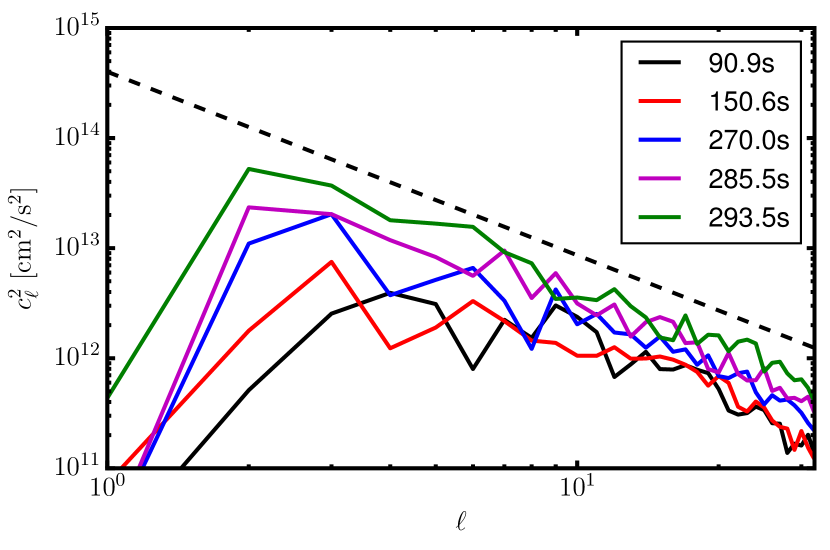
Figure 12.— Power $c_{\ell}^{2}$ in different multipoles $\ell$ for the decomposition of the radial velocity at $r=4000\,\mathrm{km}$ into spherical harmonics $Y_{\ell m}$ in the 3D model at different times computed according to Equation (30). The dominant angular wave number shifts from $\ell=3\ldots 5$ to $\ell=2$ over the course of the simulation. The dashed line indicates a slope of $\ell^{-5/3}$, which is roughly expected for a Kolmogorov spectrum above the injection scale in wave number (i.e.  at smaller spatial scales).

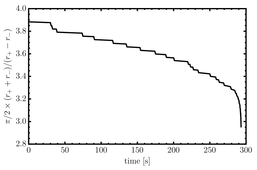
Figure 13.— Estimate of the typical angular wave number $\ell=\pi/2\times(r_{+}+r_{-})/(r_{+}-r_{-})$ of convection in the linear regime from the inner and outer boundary radius of the oxygen shell according to Equation (31) and Foglizzo et al. (2006). The rapid drop at the end of the simulation is evident and suggests that the emergence of a global $\ell=2$ mode is due to the rapid contraction of the iron and silicon core shortly before collapse.

3.3. Scale of Convective Eddies

The role of progenitor asphericities in the explosion mechanism depends not only on the magnitude of the convective velocities in the burning shells, but also on the angular scale of the infalling eddies. MLT does not make any strong assumptions about the eddy scale; it assumes a radial correlation length for entropy and velocity perturbations, but such a correlation length can in principle be realized with very different flow geometries. Empirically, simulations of buoyancy-driven convection in well-mixed shells are usually characterized by eddies of similar radial and angular extent $d$ that reach across the entire unstable zone (e.g. Arnett et al., 2009). The dominant modes are also typically close in scale to the most unstable modes in the linear regime (Chandrasekhar, 1961; Foglizzo et al., 2006), which have $d\sim r_{+}-r_{-}$. This correspondence between the linear and non-linear regime has sometimes been justified by heuristic principles for the selection of the eddy scale based on maximum kinetic energy or maximum entropy production (Malkus & Veronis, 1958; Martyushev & Seleznev, 2006). Expressing the balance of kinetic energy generation due to the growth of an instability with a scale-dependent growth rate $\omega(d)$ and turbulent dissipation for the dominant mode in a shell with mass $M$ yields

$$\dot{E}_{\mathrm{kin}}\sim\omega(d)E_{\mathrm{kin}}-v\frac{E_{\mathrm{kin}}}{d}\sim\omega(d)E_{\mathrm{kin}}-\frac{\sqrt{2}E_{\mathrm{kin}}^{3/2}}{dM^{1/2}}=0$$ (28)

for the change of the kinetic energy $E_{\mathrm{kin}}$ in a given mode. The dominant mode(s) in the non-linear regime will be the one(s) for which

$$E_{\mathrm{kin}}\propto Md^{2}\omega(d)^{2}$$ (29)

is maximal, which actually suggests a bias towards slightly larger scales than in the linear regime.

A superficial inspection of Figures 2 and 3 already reveals that our 3D models conform to the typical picture with $d\sim r_{+}-r_{-}$. More quantitatively, the dominance of large-scale modes is shown by a decomposition of the radial velocity in the inner half of the oxygen shell (at a radius of $4000\,\mathrm{km}$) into spherical harmonics (for more sophisticated decompositions of the flow field see Fernández et al. 2014; Chatzopoulos et al. 2014). In Figure 12, we plot the total power $c_{\ell}^{2}$ for each multipole order $\ell$,

$$c_{\ell}^{2}=\sum_{m=-\ell}^{\ell}\left|\int Y^{*}_{\ell m}(\theta,\varphi)v_{r}(4000\,\mathrm{km},\theta,\varphi)\,\mathrm{d}\Omega\right|^{2},$$ (30)

which shows a clear peak at low $\ell$ that slowly moves from $\ell=4$ down to $\ell=2$ over the course of the simulation. The tail at high $\ell$ above the typical eddy scale roughly exhibits an $\ell^{-5/3}$ slope as expected for a Kolmogorov-like turbulent cascade (Kolmogorov, 1941) because of the rough proportionality between $\ell$ and the wave number (Peebles, 1993).

The dominant eddy scale is consistent with the crude estimate that the dominant $\ell$ is given by the number of convective eddies of diameter $d=r_{+}-r_{-}$ that can be fitted into one hemisphere of the convective shell (Foglizzo et al., 2006),

$$\ell=\frac{\pi(r_{+}+r_{-})}{2(r_{+}-r_{-})}.$$ (31)

This estimate for the dominant multipole order is plotted in Figure 13. It agrees well with spectra of the radial velocity, although it may not clearly predict the emergence of the dominant quadrupole at the end (which is compatible with our argument that the dominant angular scale for fully developed convection is slightly larger than in the linear regime). The slowly changing geometry of the shell evidently accounts nicely for the secular trend towards modes of lower $\ell$. Figure 8 reveals that both the contraction of the inner boundary of the shell by about one third in radius and a secular expansion of the (somewhat ill-defined) outer shell boundary contribute to this trend. The fast change of $\ell$ right before collapse is clearly due to the contraction, however, as the outer boundary radius decreases again shortly before collapse.

The expansion of the outer boundary is not seen in the Kepler model and is the result of entrainment of material from the carbon shell (see Section 3.4 below). If the amount of entrainment is physical, this is another reason to suspect that estimates of the dominant angular scale based on stellar evolution models using Equation (31) will slightly overestimate the dominant $\ell$. Considering uncertainties and progenitor variations in the shell structure, Equation (31) nonetheless furnishes a reasonable zeroth-order estimate of the typical eddy scale.

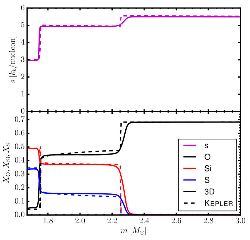
Figure 14.— Spherically averaged profiles of the entropy (violet curves, top panel) and the mass fractions of oxygen (black), silicon (red), and sulfur (blue) in the 3D run (solid curves) at $210\,\mathrm{s}$ compared to profiles from the 1D Kepler model (dashed) at the same time. Note that the slope in the mass fractions is somewhat steeper in the Kepler model, which we ascribe to the use of an extra factor of $1/3$ in the diffusion equation for compositional mixing.

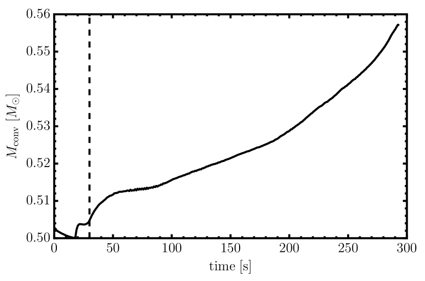
Figure 15.— Mass $M_{\mathrm{conv}}$ contained in the convective oxygen shell in the 3D simulation as a function of time. The mass increases by about $0.05M_{\odot}$ due to entrainment, which accelerates slightly towards the end of the simulation as a result of higher convective velocities and Mach numbers. Note that the small changes in the first $\mathord{\sim}30\,\mathrm{s}$ are simply due to the advection of the entropy discontinuities over the grid in the wake of hydrostatic adjustment, as a result of which cells can jump around the threshold entropies of $3.6k_{b}/\mathrm{nucleon}$ and $5.2k_{b}/\mathrm{nucleon}$ that we use to define the shell boundaries. “Physical” entrainment begins once the first convective plumes reach the boundary between the carbon and oxygen shell around $\mathord{\sim}30\,\mathrm{s}$ (denoted by a vertical line).

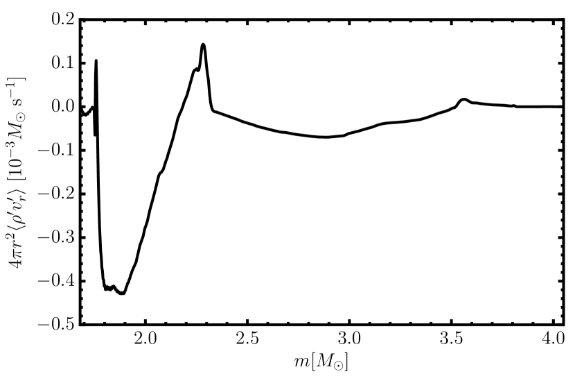
Figure 16.— Turbulent mass flux $4\pi r^{2}\langle\rho^{\prime}v^{\prime}_{r}\rangle$ in the 3D model at a time of $210\,\mathrm{s}$ as a function of enclosed mass $m$. Positive values around the outer boundary of the oxygen shell at $m\approx 2.3M_{\odot}$ indicate entrainment of material from the carbon shell. The peak value of $1.4\times 10^{-4}M_{\odot}\,\mathrm{s}^{-1}$ roughly corresponds to the average entrainment rate over the course of the simulation.

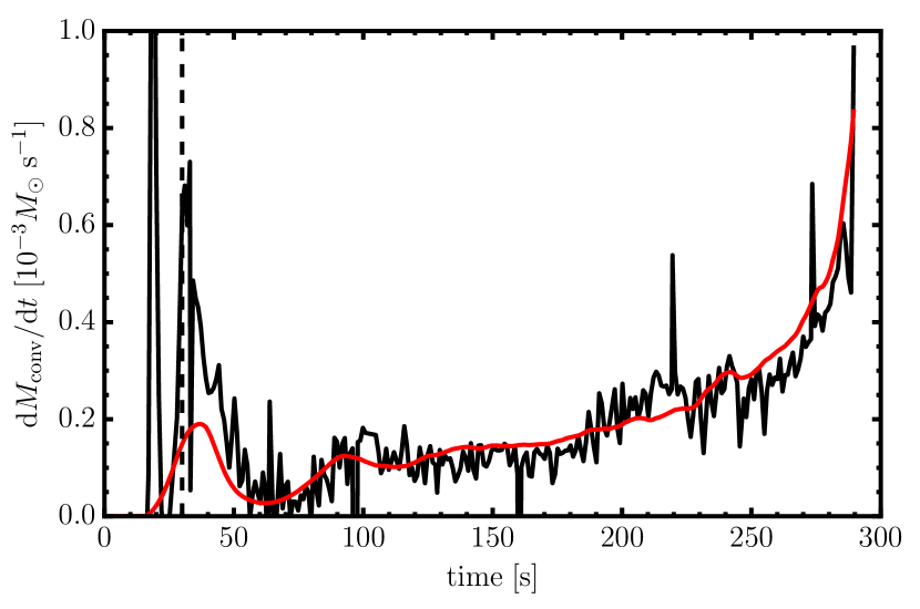
Figure 17.— Comparison of the measured entrainment rate $\dot{M}_{\mathrm{conv}}$ in the 3D simulation (black) and a fit based on Equation (32) (red) computed using $A=0.37$ and a global average for the convective velocity (see text for details). Overall, the time-dependent entrainment rate nicely follows Equation (32). Note that no data is shown later than $290\,\mathrm{s}$, as the detection of the outer boundary of the oxygen shell becomes problematic due to increasingly violent boundary mixing shortly before collapse. As in Figure 15, the dashed vertical line indicates the time when convective plumes first encounter the outer boundary and physical entrainment begins.

3.4. Comparison of Convective Mixing in 1D and 3D

Although the properties of the velocity field are more directly relevant for the potential effect of progenitor asphericities on supernova shock revival, some remarks about convective mixing in our 3D model are still in order.

In Figure 14, we compare spherically averaged profiles of the entropy $s$, and the mass fractions of oxygen, silicon, and sulphur ($X_{\mathrm{O}}$, $X_{\mathrm{Si}}$, and $X_{\mathrm{S}}$) from the 3D model to the Kepler run at a time of $210\,\mathrm{ms}$. Although the treatment of convective mixing as a diffusive process in 1D has sometimes been criticized (Arnett et al., 2009), the differences in the interior of the oxygen shell remain minute; the most conspicuous among them are the somewhat steeper gradients in the mass fractions in Kepler. These could potentially contribute (on a very modest level) to the lower total nuclear energy generation rate in Kepler, since the nuclear energy generation rate is roughly proportional to the square of the mass fraction $X_{\mathrm{O}}$ of oxygen in the burning region. Even if we account for spatial fluctuations in the composition by computing $\langle X_{\mathrm{O}}^{2}\rangle$, the compositional differences do no appear to be sufficiently large to explain the different burning rates; temperature changes due to hydrostatic adjustment thus seem to be the major cause of the somewhat higher total nuclear energy generation rate in Prometheus.

It is unclear whether the composition gradients are really an artifact of MLT; we find it equally plausible that they simply stem from the choices of different coefficients $\alpha_{2}$ and $\alpha_{3}$ for energy transport and compositional mixing in Equation (4) and (7). The introduction of an additional factor of $1/3$ in Equation (7) is typically justified by interpreting turbulent mixing as a random walk process of convective blobs with a mean free path $\Lambda_{\mathrm{mix}}$ and a total velocity $v_{\mathrm{conv}}$ with random orientation, which translates into a radial correlation length $\Lambda_{\mathrm{mix}}/\sqrt{3}$ and an RMS-averaged radial velocity of $\langle v_{r}^{2}\rangle^{1/2}=v_{\mathrm{conv}}/\sqrt{3}$. However, the mixing length and MLT velocity are implicitly identified with the radial correlation length and $\langle v_{r}^{2}\rangle^{1/2}$ in Equation (4) already, so that the choice $\alpha_{3}=\alpha_{2}$ rather than $\alpha_{3}=\alpha_{2}/3$ is arguably more appropriate. With such a (more parsimonious) choice of parameters, the composition gradients would be flattened considerably.

Figure 14 also shows evidence of boundary mixing (entrainment; Fernando, 1991; Strang & Fernando, 2001; Meakin & Arnett, 2007b) that is not captured in the Kepler run. The fact that the entropy and composition gradients are smeared out at the boundaries (especially at the outer boundary) is mostly due to the aspherical deformation of the shell interface by Kelvin-Helmholtz/Holmböe waves; the shell boundary remains relatively well defined in the multi-D snapshots in Figures 2 and 3. However, the oxygen shell is clearly expanding in $m$ at the outer boundary. To capture the increase of the total mass $M_{\mathrm{conv}}$ in the convective oxygen shell, we integrate the mass in all zones with entropies between $3.6k_{b}/\mathrm{nucleon}$ and $5.2k_{b}/\mathrm{nucleon}$ (Figure 15). $M_{\mathrm{conv}}$ increases by about $0.05M_{\odot}$ over the course of the simulation with some evidence for higher $\dot{M}_{\mathrm{conv}}$ towards the end, corresponding to an entrainment rate of $1.4\times 10^{-4}M_{\odot}$, which is also roughly the maximum value of the turbulent mass flux $4\pi r^{2}\langle\rho^{\prime}v_{r}^{\prime}\rangle$ that is reached in the formally stable region around the outer boundary (Figure 16).

Higher resolution is ultimately required to decide whether this entrainment rate is physical or partially due to numerical diffusion, which could lead to an overestimation of the amount of entrained mass in wave breaking events (see Appendix B) . Our simulations are, however, consistent with semi-empirical entrainment laws found in the literature. Laboratory experiments and simulations (Fernando, 1991; Strang & Fernando, 2001; Meakin & Arnett, 2007b) suggest

$$\dot{M}_{\mathrm{conv}}=4\pi r^{2}\rho v_{\mathrm{conv}}A\,\mathrm{Ri}_{\mathrm{B}}^{-1},$$ (32)

for the entrainment rate in the relevant regime of the bulk Richardson number $\mathrm{Ri}_{\mathrm{B}}$ and a dimensionless proportionality constant $A$. $\mathrm{Ri}_{\mathrm{B}}$ is defined in terms of the density contrast $\delta\rho/\rho$ at the interface, the gravitational acceleration $g$, the typical convective velocity $v_{\mathrm{conv}}$, and the eddy scale $\Lambda$ as

$$\mathrm{Ri}_{\mathrm{B}}=\frac{\delta\rho}{\rho}\frac{g\Lambda}{v_{\mathrm{conv}}^{2}}.$$ (33)

If we identify $\Lambda$ with the pressure scale height, this amounts to

$$\mathrm{Ri}_{\mathrm{B}}=\frac{\delta\rho}{\rho}\frac{P}{\rho v_{\mathrm{conv}}^{2}}.$$ (34)

In our case, we have $\delta\rho/\rho=0.1$, and with $v_{\mathrm{conv}}=2.5\times 10^{7}\,\mathrm{cm}\,\mathrm{s}^{-1}$ (corresponding to the non-radial velocities near the boundary, which are relevant for the dynamics of interfacial Holmböe/Kelvin-Helmholtz waves), we obtain $\mathrm{Ri}_{\mathrm{B}}=17$, indicating a very soft boundary. Together with an average convective velocity of $\mathord{\sim}200\,\mathrm{km}\,\mathrm{s}^{-1}$ and an average entrainment rate of $1.4\times 10^{-4}M_{\odot}$, this points to a low $A\sim 0.1$ in the entrainment law (32), although the ambiguities inherent in the definition of $\mathrm{Ri}_{\mathrm{B}}$ can easily shift this by an order of magnitude, which may account for the higher value $A\approx 1$ obtained by Meakin & Arnett (2007b). It is obvious that the calibration of the entrainment law is fraught with ambiguities: If we calibrate Equation (32) by using a global average for $v_{\mathrm{conv}}$,

$$v_{\mathrm{conv}}=\sqrt{\frac{2E_{\mathrm{kin},r}}{M_{\mathrm{conv}}}},$$ (35)

and the initial values for $\delta\rho/\rho$, and the density $\rho$ at the outer boundary radius $r$ in (32) and (34), the time-dependent entrainment rate is well fitted by $A=0.37$ (Figure 17). If anything, relatively low values of $A$ merely demonstrate that entrainment in our 3D model is no more affected by numerical diffusion than in comparable simulations. Considering the low value of the bulk Richardson number and the small entropy jump of $\sim 0.5k_{b}/\mathrm{nucleon}$, which should be conducive to entrainment effects, the dynamical impact of boundary mixing in our simulation is remarkably small, but its long-term effect warrants further investigation.

4. Requirements for 3D Pre-Supernova Simulations

If 3D simulations of shell burning in massive stars are to be used as input for core-collapse simulations, it is essential that the typical convective velocities and eddy scales are captured accurately. The analysis of our model in the preceding section provides guidelines about the approximations that can (or cannot) be justified in such simulations.

The emergence of large-scale motions ($\ell=2$ modes) during the final phase of our model implies that pre-SN model generally need to cover the full solid angle (which has been done previously for oxygen shell burning only by Kuhlen et al. 2003, albeit for an earlier phase). However, for sufficiently narrow convective shells, simulations restricted to a wedge or octant may still cover the flow geometry accurately notwithstanding that such symmetry assumptions remain questionable in the ensuing SN phase. Thus, for the pre-SN phase, the assumption of octant symmetry in Couch et al. (2015) may be adequate for their model of silicon shell burning, which has $r_{+}/r_{-}\approx 2$ towards the end of the simulation. The eddies should then remain of a moderate scale with a preferred $\ell$ of $\ell\approx\pi/2(r_{+}+r_{-})/(r_{+}-r_{-})=4.71$.

An accurate treatment of nuclear burning is even more critical because of the scaling of convective velocities with $(\dot{Q}_{\mathrm{nuc}}/M_{\mathrm{conv}})^{1/3}$. Since the nuclear generation rates in the silicon and oxygen shell are sensitive to the contraction of the deleptonizing iron core, this not only applies to the burning shell in question itself, but also to the treatment applied for the iron core. If the contraction of the core is artificially accelerated as in Couch et al. (2015), this considerably reduces the nuclear time-scale in the outer shells as well. For example $\mathord{\sim}0.2M_{\odot}$ of intermediate mass-elements in the silicon shell are burned to iron group elements within $160\,\mathrm{s}$ in the 3D model of Couch et al. (2015), i.e.  silicon burning on average proceeds $6.25$ times faster than in the corresponding stellar evolution model, where this takes $1000\,\mathrm{s}$. This suggests an artificial increase of the convective velocities by $84\%$ in their 3D model.

Approximations that affect the nuclear burning time-scale are also problematic because they change the ratio $\tau_{\mathrm{conv}}/\tau_{\mathrm{nuc}}\propto\tau_{\mathrm{nuc}}^{-2/3}$, which plays a crucial role in the freeze-out of convective motions shortly before the onset of collapse (see Section 3.2). If the nuclear burning is artificially accelerated and continues until collapse, then the freeze-out will occur somewhat earlier, which may compensate the overestimation of convective velocities discussed before. However, the simulation of Couch et al. (2015) suggests that the opposite may also occur: In their 3D model, silicon burning slows down towards the end of their simulation as the shell almost runs out of fuel. In the corresponding 1D stellar evolution model, convection in the original silicon shell has already died down completely as can be seen from their Figure 2, which shows non-zero convective velocities only in regions with $Y_{e}=0.5$. While it is conceivable that convection subsides more gradually in 3D as the available fuel is nearly consumed – probably over a few turnover time-scales – increasing the ratio $\tau_{\mathrm{conv}}/\tau_{\mathrm{nuc}}$ by more than a factor of $\gtrsim 3$ evidently introduces the risk of artificially prolonging convective activity in almost fully burned shells.

Other worries about the feasibility of multi-D simulations of supernova progenitors include the problem of thermal adjustment after mapping from a 1D stellar evolution model as well as artificial boundary mixing. We have largely circumvented the problem of thermal adjustment in this study by focusing on the final stages. The somewhat higher nuclear burning rate in the 3D model (by up to $\mathord{\sim}50\%$ compared to Kepler), which may be due to physical multi-D effects or transients after the mapping such as an adjustment to a new hydrostatic equilibrium, suggests that even for a setup where the problem of hydrostatic and thermal adjustment is rather benign, we still face uncertainties of the order of $15\%$ – because of $v_{\mathrm{conv}}\propto(\dot{Q}_{\mathrm{nuc}}/\mathrm{M}_{\mathrm{conv}})^{1/3}$ – in the final convective velocity field at collapse. The slight expansion of the outer boundary of the oxygen shell, which may be the result of an adjustment effect or driven by (physical) entrainment, also deserves attention because it plays some role in fostering the emergence of an $\ell=2$ mode right before collapse. It appears less worrisome, however, since there are natural variations in shell geometry anyway, and since the emergence of the $\ell=2$ mode may still be primarily driven by the contraction of inner shell boundary. There is no evidence for artificial boundary mixing at this stage, although further high-resolution tests remain desirable.

5. Effect of Convective Seed Perturbations on Supernova Shock Revival

With typical convective Mach numbers of $\sim 0.1$ and a dominant $\ell=2$ mode at collapse, the progenitor asphericities fall in the regime where they may be able to affect shock revival in the ensuing core-collapse supernova, as has been established by the parameter study of Müller & Janka (2015). Considering that several recent works have shown that the conditions for shock revival in multi-D can be captured with good accuracy by surprisingly simple scaling laws (Müller & Janka, 2015; Summa et al., 2016; Janka et al., 2016; Müller et al., 2016) that generalize the concept of the critical luminosity (Burrows & Goshy, 1993) to multi-D, it is reasonable to ask whether the effect of progenitor asphericities can also be predicted more quantitatively by simple analytic arguments. Given the good agreement between our 3D model and MLT, such a theory could help to better identify progenitors for which convective seed asphericities play a major role in the explosion before investing considerable computer time into multi-D simulations.

The key ingredient to accomplish this consists in a first quantitative theory for the interaction of asymmetries in the supersonic infall region with the shock, which Müller & Janka (2015) only described qualitatively as “forced shock deformation”. The starting point is the translation of initial radial velocity perturbations into density perturbations at the shock due to differential infall (Müller & Janka, 2015),

$$\delta\rho_{\mathrm{pre}}/\rho_{\mathrm{pre}}\approx\mathrm{Ma},$$ (36)

which can also be understood more rigorously using linear perturbation theory (Goldreich et al., 1997; Takahashi & Yamada, 2014). Note that we now designate the typical convective Mach number during convective shell burning simply as $\mathrm{Ma}$ to avoid cluttered notation. The perturbations in the transverse velocity components are amplified as $r^{-1}$ (Goldreich et al., 1997) and are roughly given by

$$\delta v_{t}\approx\mathrm{Ma}\,c_{\mathrm{s,ini}}(r_{\mathrm{ini}}/r_{\mathrm{sh}}),$$ (37)

where $c_{\mathrm{s,ini}}$ and $r_{\mathrm{ini}}$ are the initial sound speed and radius of the shell before collapse and $r_{\mathrm{sh}}$ is the shock radius. Radial velocity perturbations only grow with $r^{-1/2}$ (Goldreich et al., 1997) and can therefore be neglected.

5.1. Generation of Turbulent Kinetic Energy by Infalling Perturbations

The interaction of the pre-shock perturbations with the shock can then be interpreted as an injection of additional turbulent kinetic energy into the post-shock region. While this problem has not yet been addressed in the context of spherical accretion onto a neutron star, the interaction of planar shocks with incident velocity and density perturbations has received some attention in fluid dynamics (Ribner, 1987; Andreopoulos et al., 2000; Wouchuk et al., 2009; Huete Ruiz de Lira, 2010; Huete et al., 2012). The perturbative techniques that allow a relatively rigorous treatment in the planar case cannot be replicated here, and we confine ourselves to simple rule-of-thumb estimate for the generation of turbulent energy by the infalling perturbations: If we neglect the deformation of the shock initially, we can assume transverse velocity perturbations $\delta v_{\mathrm{t}}$ and density fluctuations $\delta\rho/\rho$ compared to the spherically averaged flow are conserved across the shock as a first-order approximation. The anisotropy of the ram pressure will also induce pressure fluctuations $\delta P/P\sim\delta\rho/\rho$ downstream of the shock. In a more self-consistent solution, these pressure fluctuations would induce lateral flows and modify the shape of the shock, and larger vorticity perturbations would arise if the shock is asymmetric to begin with (which is important in the context of the SASI (Foglizzo et al., 2007; Guilet & Foglizzo, 2012). As a crude first-order estimate such a rough estimate is sufficient for our purpose; it is not incompatible with recent results about shocks traveling in inhomogeneous media (Huete Ruiz de Lira, 2010; Huete et al., 2012).

From the density and pressure perturbations $\delta\rho/\rho\sim\delta P/P\mathord{\sim}\mathrm{Ma}$ and transverse velocity perturbations $\delta v_{t}\sim\mathrm{Ma}\,c_{\mathrm{s,ini}}(r_{\mathrm{ini}}/r_{\mathrm{sh}})$ downstream of the shock, we can estimate fluxes of transverse kinetic energy ($F_{\mathrm{t}}$), acoustic energy ($F_{\mathrm{ac}}$), and an injection rate of kinetic energy due to the work done by buoyancy during the advection of the accreted material through down to the gain radius $r_{\mathrm{g}}$. $F_{\mathrm{t}}$ is roughly given by,

$$F_{\mathrm{t}} = \frac{\dot{M}}{2}\delta v_{\mathrm{t}}^{2}=\frac{\dot{M}}{2}\mathrm{Ma}^{2}c_{\mathrm{s,ini}}^{2}\left(\frac{r_{\mathrm{ini}}}{r_{\mathrm{sh}}}\right)^{2}$$

$$\approx \mathrm{Ma}^{2}\frac{GM\dot{M}}{6r_{\mathrm{ini}}}\left(\frac{2r_{\mathrm{ini}}^{2}}{3r_{\mathrm{g}}r_{\mathrm{sh}}}\right)=\mathrm{Ma}^{2}\frac{GM\dot{M}}{9r_{\mathrm{g}}}\left(\frac{r_{\mathrm{ini}}}{r_{\mathrm{sh}}}\right),$$

where we approximated the initial sound speed as $c_{\mathrm{s,ini}}^{2}\approx GM/(3r_{\mathrm{ini}})$, which is a good approximation for the shells outside the iron core. Note that we use a typical ratio $r_{\mathrm{sh}}/r_{\mathrm{g}}=3/2$ during the pre-explosion phase to express $F_{\mathrm{t}}$ in terms of the gravitational potential of the gain radius; the reason for this will become apparent when we compare the injection rate of turbulent kinetic energy at the shock to the contribution from neutrino heating.

Following Landau & Lifshitz (1959), the acoustic energy flux can be estimated by assuming that the velocity fluctuations in acoustic waves are roughly $\delta v\sim c_{s}\delta P/P$ (where $c_{s}$ is the sound speed behind the shock and $\delta P\approx\mathrm{Ma}\,P$). The post-shock pressure $P$ can be determined from the jump conditions,

$$P=\rho_{\mathrm{pre}}\frac{\beta-1}{\beta}v_{\mathrm{pre}}^{2}=\rho\frac{\beta-1}{\beta^{2}}\frac{GM}{r_{\mathrm{sh}}},$$ (39)

where $\rho_{\mathrm{pre}}$ and $\rho$ are the pre- and post-shock density, $\beta\approx 7$ is the compression ratio in the shock, and $v_{\mathrm{pre}}$ is the pre-shock velocity, which we approximate as $v_{\mathrm{pre}}=\sqrt{GM/r_{\mathrm{sh}}}$. The acoustic energy flux is thus,

$$F_{\mathrm{ac}} = 4\pi r_{\mathrm{sh}}^{2}\delta P\,\delta v=4\pi r_{\mathrm{sh}}^{2}\frac{\delta P^{2}c_{s}}{P}=4\pi\rho|v_{r}|r_{\mathrm{sh}}^{2}\frac{\delta P^{2}c_{s}}{\rho P|v_{r}|}$$ (40)

$$= 4\pi\rho|v_{r}|r_{\mathrm{sh}}^{2}\frac{\mathrm{Ma}^{2}c_{s}P}{\rho|v_{r}|}=\dot{M}\,\mathrm{Ma}^{2}\frac{\beta-1}{\beta^{2}}\frac{GM}{r_{\mathrm{sh}}}\frac{\beta}{\sqrt{3}}$$

$$\approx 0.49\mathrm{Ma}^{2}\frac{GM\dot{M}}{r_{\mathrm{g}}}.$$

Here, $|v_{r}|=v_{\mathrm{pre}}/\beta$ is the spherical average of the post-shock velocity, and $c_{s}^{2}\approx GM/(3r_{\mathrm{sh}})$ has been used following Müller & Janka (2015).

Finally, the gravitational potential energy corresponding to density fluctuations $\delta\rho$ will be converted into kinetic energy by buoyancy forces at a rate of

$$F_{\mathrm{pot}} = \frac{\dot{M}\delta\rho}{\rho}\left(\frac{GM}{r_{\mathrm{sh}}}-\frac{GM}{r_{\mathrm{g}}}\right)=\mathrm{Ma}\,\dot{M}\left(\frac{GM}{r_{\mathrm{g}}}-\frac{GM}{r_{\mathrm{sh}}}\right)$$ (41)

$$\approx \mathrm{Ma}\frac{GM\dot{M}}{3r_{\mathrm{g}}}.$$

Especially for moderate Mach numbers, $F_{\mathrm{pot}}$ is clearly the dominating term, as the flux of acoustic and transverse kinetic energy scale with $\mathrm{Ma}^{2}$.

In the absence of infalling perturbations, Müller & Janka (2015) established a semi-empirical scaling law that relates transverse kinetic energy $E_{\mathrm{kin,t}}$ stored in the post-shock region to the volume-integrated neutrino heating rate $\dot{Q}_{\nu}$, the mass in gain region, $M_{\mathrm{g}}$, and the shock and gain radius,

$$\frac{E_{\mathrm{kin,t}}}{M_{\mathrm{g}}}\approx\frac{1}{2}\left[\frac{(r_{\mathrm{sh}}-r_{\mathrm{g}})\dot{Q}_{\nu}}{M_{\mathrm{g}}}\right]^{2/3}.$$ (42)

At least for convection-dominated models, this scaling law can be understood as the result of a balance between kinetic energy generation by buoyancy and turbulent dissipation with a dissipation length $\Lambda=r_{\mathrm{sh}}-r_{\mathrm{g}}$ (cf.  also Murphy et al. 2013). Assuming a local dissipation rate of $v^{3}/\Lambda=(2E_{\mathrm{kin,t}}/M_{\mathrm{g}})^{3/2}/\Lambda$, this leads to

$$\dot{E}_{\mathrm{kin,t}}=\dot{Q}_{\nu}-\frac{1}{\Lambda}\left(\frac{2E_{\mathrm{kin,t}}}{M_{\mathrm{g}}}\right)^{3/2}M_{\mathrm{g}}=0,$$ (43)

from which Equation (42) immediately follows.

In the presence of infalling perturbations, it is natural to add another source term to Equation (43),

$$\dot{Q}_{\nu}+F_{\mathrm{pot}}-\frac{1}{\Lambda}\left(\frac{2E_{\mathrm{kin,t}}}{M_{\mathrm{g}}}\right)^{3/2}M_{\mathrm{g}}=0.$$ (44)

To keep the calculation tractable, we only include the dominant contribution $F_{\mathrm{pot}}$ arising from infalling perturbations and discard $F_{\mathrm{ac}}$ and $F_{\mathrm{t}}$.

However, this obviously poses the question about the appropriate choice for $\Lambda$, which can now no longer assumed to be simply given by $r_{\mathrm{sh}}-r_{\mathrm{g}}$. To get some guidance, we can consider the limit in which neutrino heating is negligible; here the appropriate choice for $\Lambda$ is clearly given by the scale of the infalling perturbations, i.e. $\Lambda\approx\pi r_{\mathrm{sh}}/\ell$ in terms of their typical angular wave number $\ell$. Hence we find,

$$\frac{E_{\mathrm{kin,t}}}{M_{\mathrm{g}}}=\frac{1}{2}\left[\frac{\pi r_{\mathrm{sh}}F_{\mathrm{pot}}}{\ell M_{\mathrm{g}}}\right]^{2/3},$$ (45)

in this limit. The general case can be accommodated by simply interpolating between the two limits,

$$\frac{E_{\mathrm{kin,t}}}{M_{\mathrm{g}}}=\frac{1}{2}\left[\frac{(r_{\mathrm{sh}}-r_{\mathrm{g}})\dot{Q}_{\nu}}{M_{\mathrm{g}}}+\frac{\pi r_{\mathrm{sh}}F_{\mathrm{pot}}}{\ell M_{\mathrm{g}}}\right]^{2/3}.$$ (46)

We emphasize that a different dissipation length enters in both terms: In the limit of neutrino-driven convection with small seed perturbations, the dissipation length is given by the width of the gain layer, whereas the dissipation length $\pi r_{\mathrm{sh}}/\ell$ can be considerably larger for “forced” convection/shock deformation due to infalling perturbations with small $\ell$.

For deriving the modification of the critical luminosity, it will be convenient to express $E_{\mathrm{kin,t}}$ in terms of its value in the limit of small seed perturbations (Equation 42) and a correction term $\psi$,

$$\frac{E_{\mathrm{kin,t}}}{M_{\mathrm{g}}}=\frac{1}{2}\left[\frac{(r_{\mathrm{sh}}-r_{\mathrm{g}})\dot{Q}_{\nu}}{M_{\mathrm{g}}}\right]^{2/3}(1+\psi)^{2/3},$$ (47)

where $\psi$ is defined as

$$\psi=\frac{\pi r_{\mathrm{sh}}F_{\mathrm{pot}}/(\ell M_{\mathrm{g}})}{(r_{\mathrm{sh}}-r_{\mathrm{g}})\dot{Q}_{\nu}/M_{\mathrm{g}}}=\frac{\pi r_{\mathrm{sh}}F_{\mathrm{pot}}}{\ell(r_{\mathrm{sh}}-r_{g})\dot{Q}_{\nu}}.$$ (48)

Different from the case of negligible seed perturbations, it is hard to validate Equation (46) in simulations. In the 2D study of Müller & Janka (2015), the amplitudes of the infalling perturbations change significantly over relatively short time-scales, and the phase during which they have a significant impact on the turbulent kinetic energy in the post-shock region but have not yet triggered shock revival was therefore too short to detect any deviations from Equation (42), especially since the turbulent kinetic energy fluctuates considerably around its saturation value in 2D.

5.2. Effect on the Heating Conditions and the Critical Luminosity

Conceptually, the steps from Equation (46) to a modified critical luminosity are no different from the original idea of Müller & Janka (2015), i.e.  one can assume that the average shock radius can be obtained by rescaling the shock radius $r_{\mathrm{sh,1D}}$ for the stationary 1D accretion problem with a correction factor that depends on the average RMS Mach number $\langle\mathrm{Ma}_{\mathrm{gain}}^{2}\rangle$ in the gain region (Equation 42 in Müller & Janka 2015),

$$r_{\mathrm{sh}}\approx r_{\mathrm{sh,1D}}\left(1+\frac{4}{3}\langle\mathrm{Ma}_{\mathrm{gain}}^{2}\rangle\right)^{2/3},$$ (49)

which then leads to a similar correction factor for the critical values for the neutrino luminosity and mean energy $L_{\nu}$ and $E_{\nu}$ (Equation 41 in Müller & Janka 2015).

In the presence of strong seed perturbations, we can express $\langle\mathrm{Ma}_{\mathrm{gain}}^{2}\rangle$ at the onset of an explosive runaway in terms of its value $\langle\mathrm{Ma}_{\nu}^{2}\rangle$ at shock revival in the case of small seed perturbations and a correction factor $(1+\psi)^{2/3}$ as in Equation (46),

$$L_{\nu}E_{\nu}^{2}\propto(\dot{M}M)^{3/5}r_{\mathrm{g}}^{-2/5}\left[1+\frac{4}{3}\langle\mathrm{Ma}_{\nu}^{2}\rangle(1+\psi)^{2/3}\right]^{-3/5}.$$ (50)

Equation (50) obviously hinges on the proper calibration (and validation) of Equation (46), which needs to be provided by future core-collapse supernova simulations. Nonetheless, it already allows some crude estimates.

The ratio of the critical luminosity with strong seed perturbation $(L_{\nu}E_{\nu}^{2})_{\mathrm{pert}}$ to the critical luminosity $(L_{\nu}E_{\nu}^{2})_{\mathrm{3D}}$ value in multi-D for small seed perturbations is found to be

$$\frac{(L_{\nu}E_{\nu}^{2})_{\mathrm{pert}}}{(L_{\nu}E_{\nu}^{2})_{\mathrm{3D}}} = \left(\frac{1+4/3\langle\mathrm{Ma}_{\nu}^{2}\rangle(1+\psi)^{2/3}}{1+4/3\langle\mathrm{Ma}_{\nu}^{2}\rangle}\right)^{-3/5}$$ (51)

$$\approx 1-\frac{8\langle\mathrm{Ma}_{\nu}^{2}\rangle\psi}{15\big{(}1+4/3\langle\mathrm{Ma}_{\nu}^{2}\rangle\big{)}},$$

where we linearized in $\psi$. In order not to rely on an increasingly long chain of uncertain estimates, it is advisable to use the known multi-D effects without strong seed perturbations as a yardstick; they bring about a reduction of the critical luminosity by about $25\%$ compared to 1D (Murphy & Burrows, 2008; Hanke et al., 2012; Couch, 2013; Dolence et al., 2013; Müller & Janka, 2015). This reduction is obtained by setting $\mathrm{Ma}_{\nu}^{2}=0.4649$ at the onset of runaway shock expansion, which is also the value derived by Müller & Janka (2015) based on analytic arguments.

Using this value, we estimate a reduction of the critical luminosity by $\mathord{\sim}0.15\psi$ relative to the the critical luminosity in multi-D without perturbations, which remains only a very rough indicator for the importance of perturbations in shock revival barring any further calibration and a precise definition of how and where $\mathrm{Ma}$ is to be measured.

It is illustrative to express $\psi$ in terms of the heating efficiency $\eta_{\mathrm{heat}}$, which is defined as the ratio of the volume-integrated neutrino heating rate and the sum of the electron neutrino and antineutrino luminosities $L_{\nu_{e}}$ and $L_{\bar{\nu}_{e}}$,

$$\eta_{\mathrm{heat}}=\frac{\dot{Q}_{\nu}}{L_{\nu_{e}}+L_{\bar{\nu}_{e}}},$$ (52)

and the accretion efficiency $\eta_{\mathrm{acc}}$,

$$\eta_{\mathrm{acc}}=\frac{L_{\nu_{e}}+L_{\bar{\nu}_{e}}}{GM\dot{M}/r_{\mathrm{g}}}.$$ (53)

We then obtain

$$\psi=\frac{\pi r_{\mathrm{sh}}\mathrm{Ma}}{3\ell(r_{\mathrm{sh}}-r_{\mathrm{g}})\eta_{\mathrm{acc}}\eta_{\mathrm{heat}}}\approx\frac{\pi\mathrm{Ma}}{\ell\eta_{\mathrm{acc}}\eta_{\mathrm{heat}}}.$$ (54)

Using Equation (54), we can verify that the estimated reduction of the critical luminosity due to seed perturbations by $\mathord{\sim}0.15\psi$ is in the ballpark: If we take $\mathrm{Ma}$ to be half the maximum value of the Mach number in the infalling shells in the models of Müller & Janka (2015) and work with reasonable average values of $\eta_{\mathrm{acc}}=2$ and $\eta_{\mathrm{heat}}=0.05$, we obtain a reduction of 11% for their model p2La0.25 ($\mathrm{Ma}=0.045$), 24% for p2La1 ($\mathrm{Ma}=0.1$), and 36% for p2La2 ($\mathrm{Ma}=0.15$), which agrees surprisingly well with their inferred reduction of the critical luminosity (Figure 12 in their paper). It also explains why their models with $\ell=4$ require twice the convective Mach numbers in the oxygen shell to explode at the same time as their corresponding $\ell=2$ models. For the models of Couch & Ott (2013, 2015) with $\eta_{\mathrm{heat}}\approx 0.1$ and $\ell=4$, our estimate would suggest a reduction in critical luminosity by 6%. This prediction cannot be compared quantitatively to the results of Couch & Ott (2013, 2015) since an analysis of the effect on the critical luminosity in the vein of Müller & Janka (2015) and Summa et al. (2016) would require additional data (e.g., trajectories of the gain radius). Qualitatively, such a moderate reduction of the critical luminosity seems consistent with their results: The effect of infalling perturbations corresponds to a change in the critical heating factor (by which they multiply the critical luminosity to compute the neutrino heating terms) by only $2\ldots 3\%$, and their inferred reduction of the “critical heating efficiency” by $\mathord{\sim}10\%$ due to infalling perturbations is much smaller than the reduction of the critical heating efficiency by a factor of $\mathord{\sim}2$ in 3D compared to 1D. For the simulations of Couch et al. (2015), for which we estimate the convective Mach number in the silicon shell as roughly $0.02$, the expected reduction in the critical luminosity (again for $\eta_{\mathrm{heat}}\approx 0.1$ and a dominant $\ell=4$ mode) is roughly $1\%$ , which is consistent with the development of an explosion in both the perturbed and the unperturbed model.

For our $18M_{\odot}$ progenitor model with a typical convective Mach number $\mathrm{Ma}\approx 0.1$ in the middle of the oxygen shell, we expect a much more sizable reduction of the critical luminosity by $12\ldots 24\%$ if we assume $\eta_{\mathrm{acc}}=2$, $\ell=2$ and $\eta_{\mathrm{heat}}=0.05\ldots 0.1$, although this crude estimate still needs to be borne out by a follow-up core-collapse supernova simulation. Because the importance of the infalling perturbations relative to the contribution of neutrino heating to non-radial instabilities is determined by $\eta_{\mathrm{acc}}$ and $\eta_{\mathrm{heat}}$, reasonably accurate multi-group transport is obviously required; the inaccuracy of leakage-based models like Couch & Ott (2013) and Couch et al. (2015) that has been pointed out by Janka et al. (2016) evidently does not permit anything more than a proof of principle.

6. Summary and Conclusions

In this paper, we presented the first 3D simulation of the last minutes of oxygen shell burning outside a contracting iron and silicon core in a massive star (ZAMS mass $18M_{\odot}$) up to the onset of collapse. Our simulation was conducted using a 19-species $\alpha$-network as in the stellar evolution code Kepler (Weaver et al., 1978) and an axis-free, overset Yin-Yang grid (Kageyama & Sato, 2004; Wongwathanarat et al., 2010) to cover the full solid angle and allow for the emergence of large-scale flow patterns. To circumvent the problem of core deleptonization and nuclear quasi-equilibrium in the silicon shell without degrading the accuracy of the simulation by serious modifications of the core evolution, a large part of the silicon core was excised and replaced by a contracting inner boundary with a trajectory determined from the corresponding Kepler run. The model was evolved over almost 5 minutes, leaving ample time for transients to die down and roughly 3 minutes or 9 turnover time-scalse of steady-state convection for a sufficiently trustworthy analysis of the final phase before collapse.

For the simulated progenitor, an $18M_{\odot}$ star of solar metalicity with an extended oxygen shell, our 3D simulation shows the acceleration of convection from typical Mach numbers of $\mathord{\sim}0.05$ to $\mathord{\sim}0.1$ at collapse due to the increasing burning rate at the base of the shell. The contraction of the core also leads to the emergence of larger scales in the flow, which is initially dominated by $\ell=3$ and $\ell=4$ modes before a pronounced quadrupolar ($\ell=2$) mode develops shortly before collapse. As a result of a small buoyancy jump between the oxygen and carbon shell, the oxygen shell grows from $0.51M_{\odot}$ to $0.56M_{\odot}$ due to the entrainment of material from the overlying carbon shell over the course of the simulation, which appears compatible with empirical scaling laws for the entrainment rate at convective boundaries (Fernando, 1991; Strang & Fernando, 2001; Meakin & Arnett, 2007b).

The comparison with the corresponding Kepler model shows that – aside from entrainment at the boundaries – convection is well described by mixing length theory (MLT) in the final stage before collapse in the model studied here. MLT at least captures the bulk properties of the convective flow that matter for the subsequent collapse phase quite accurately: If properly “gauged”, the convective velocities predicted by MLT in Kepler agree well with the 3D simulation, and the time-dependent implementation of MLT even does a reasonable job right before collapse when the nuclear energy generation rate changes significantly within a turnover time-scale, which results in a “freeze-out” of convection. The good agreement with MLT is also reflected by the fact that the kinetic energy in convective motions obeys a scaling law of the expected form (Biermann, 1932; Arnett et al., 2009). The kinetic energy $E_{\mathrm{kin},r}$ in radial convective motions can be described to good accuracy in terms of the average nuclear energy generation rate per unit mass $\dot{q}_{\mathrm{nuc}}$, the pressure scale height $h_{P}$ at the base of the shell, and the mass $M_{\mathrm{conv}}$ in the shell as,

$$E_{\mathrm{kin},r}\approx 0.35M_{\mathrm{conv}}(\dot{q}_{\mathrm{nuc}}h_{P})^{2/3},$$ (55)

and the convective velocities are not too far from

$$\delta v_{r}\approx\omega_{\mathrm{BV}}h_{P},$$ (56)

where $\omega_{\mathrm{BV}}$ is the Brunt-Väisälä frequency and $h_{P}$ is the local value of the pressure scale height. Our results are consistent with the assumption that convective blobs are accelerated only over roughly one pressure scale height, and there appears to be no need to replace the pressure scale height in Equation (55) with the extent of the convective zone as the arguments of Arnett et al. (2009) suggest. We surmise that this may be a specific feature of the final phases of shell convection before collapse that requires the dissipation of turbulent energy within a limited distance: Since neutrino cooling no longer balances nuclear energy generation, the convective flow will adjust such as to maintain a constant rate of entropy generation throughout the shell to avoid a secular build-up or decline of the unstable gradient. During earlier phases with appreciable neutrino cooling in the outer regions of convective shells, Equation (55) may no longer be adequate.

Similarly, the dominant scale of the convective eddies agrees well with estimates based on linear perturbation theory (Chandrasekhar, 1961; Foglizzo et al., 2006). In terms of the radii $r_{-}$ and $r_{+}$ of the inner and outer shell boundary, the dominant angular wave number $\ell$ is roughly

$$\ell\approx\frac{\pi(r_{+}+r_{-})}{2(r_{+}-r_{-})}.$$ (57)

Our findings already allow some conclusions about one of the primary questions that has driven the quest for 3D supernova progenitors, i.e.  whether progenitor asphericities can play a beneficial role for shock revival. We suggest that Equations (55) and (57) can be used to formulate an estimate for the importance of convective seed perturbations for shock revival in the ensuing supernova (Couch & Ott, 2013; Müller & Janka, 2015; Couch et al., 2015). To this end, these two equations (or alternatively, the convective velocities obtained via MLT in a stellar evolution code) need to be evaluated at the time of freeze-out of convection to obtain the typical convective Mach number $\mathrm{Ma}$ and angular wave number $\ell$ at collapse. The time of freeze-out can be determined by equating the typical time-scale for changes in the volume-integrated burning rate $\dot{Q}_{\mathrm{nuc}}$ with the turnover time-scale $t_{\mathrm{conv}}$, which results in the condition

$$\frac{\mathrm{d}\ln\dot{Q}_{\mathrm{nuc}}}{\mathrm{d}t}=\frac{\omega_{\mathrm{BV,max}}}{2\pi},$$ (58)

or,

$$\frac{\mathrm{d}\ln\dot{Q}_{\mathrm{nuc}}}{\mathrm{d}t}=t_{\mathrm{conv}}^{-1}.$$ (59)

Relying on an estimate for the extra turbulent energy generated in the post-shock region in the supernova core by the infall of seed perturbations, and using the reduction of the energy-weighted critical neutrino luminosity $\mathcal{L}_{\mathrm{crit}}$ for explosion by $\mathord{\sim}25\%$ in multi-D (Murphy & Burrows, 2008; Hanke et al., 2012; Müller & Janka, 2015) as a yardstick, one finds that strong seed perturbations should reduce $\mathcal{L}_{\mathrm{crit}}$ further by

$$\frac{\Delta\mathcal{L}_{\mathrm{crit}}}{\mathcal{L}_{\mathrm{crit}}}\approx 0.47\frac{\mathrm{Ma}}{\ell\eta_{\mathrm{acc}}\eta_{\mathrm{heat}}},$$ (60)

relative to the control value in multi-D simulations without strong seed perturbations. Here $\eta_{\mathrm{acc}}$ and $\eta_{\mathrm{heat}}$ are the accretion and heating efficiency in the supernova core, $\mathrm{Ma}$ is the typical convective Mach number in the infalling shell at the onset of collapse, and $\mathcal{L}_{\mathrm{crit}}=(L_{\nu}E_{\nu}^{2})_{\mathrm{crit}}$ includes the proper weighting of the neutrino luminosity $L_{\nu}$ with the square of the neutrino mean energy $E_{\nu}^{2}$ (Janka, 2012; Müller & Janka, 2015). This estimate appears to be roughly in line with recent multi-D studies of shock revival with the help of strong seed perturbations and nicely accounts for the range of effect sizes from Couch et al. (2015) (no qualitative change in shock revival) to Müller & Janka (2015) (reduction of $\mathcal{L}_{\mathrm{crit}}$ by tens of percent for $\ell=2$ modes with sufficiently strong perturbations). For our 3D progenitor model, we expect a reduction of the critical luminosity by $12\ldots 24\%$.

Considering these numbers, the prospects for a significant and supportive role of progenitor asphericities in the supernova explosion mechanism seem auspicious. Yet caution is still in order. Because the relative importance of seed perturbations is determined by the ratio $\mathrm{Ma}/(\eta_{\mathrm{acc}}\eta_{\mathrm{heat}})$, a reliable judgment needs to be based both on a self-consistent treatment of convective burning in multi-D before collapse (which determines $\mathrm{Ma}$) and accurate multi-group neutrino transport after bounce (which determines $\eta_{\mathrm{acc}}$ and $\eta_{\mathrm{heat}}$). Again, first-principle models of supernovae face a curious coincidence: As one typically finds $\mathrm{Ma}\sim\eta_{\mathrm{heat}}$, progenitor asphericities are just large enough to play a significant role in the explosion mechanism, but not large enough to provide a clear-cut solution for the problem of shock revival. The danger of a simplified neutrino treatment has already been emphasized repeatedly in the literature (see Janka et al. 2016 for a recent summary), but pitfalls also abound in simulations of convective burning: For example, the recipes employed by Couch et al. (2015) can be shown to considerably affect the convective Mach number at collapse by appealing to scaling laws from MLT and time-scale considerations.

Our method of excising the core seems to be a viable avenue towards obtaining 3D initial conditions in the oxygen shell (which is the innermost active convective shell in many progenitor models) without introducing inordinate artifacts due to initial transients or artificial changes to the nuclear burning. Nonetheless, the model presented here is only another step towards a better understanding of the multi-D structure of supernova progenitors. In particular, the effects of resolution and stochasticity on the convective flow need to be studied in greater depth, though a first restricted resolution study (Appendix B) suggests that the predicted convective velocities are already accurate to within $10\%$ or less.

Future simulations will also need to address progenitor variations in the shell geometry, shell configuration, and the burning rate; in fact the $18M_{\odot}$ was deliberately chosen as an optimistic case with strong oxygen burning at the base of a very extended convective shell, and may not be representative of the generic situation (if there is any). Moreover, massive stars with active convective silicon shells at collapse also need to be explored even if they form just a subclass of all supernova progenitors. Treating this phase adequately to avoid the artifacts introduced by an approach like that of Couch et al. (2015) is bound to prove a harder challenge due to the complications of nuclear quasi-equilibrium. Finally, the long-term effects of entrainment and other phenomena that cannot be captured by MLT need to be examined: If such effects play a major role in the evolution of supernova progenitors, capturing them with the help of exploratory 3D models and improved recipes for 1D stellar evolution in the spirit of the 321D approach (Arnett et al., 2015) will be much more challenging than 3D simulations of the immediate pre-collapse stage, where the problems of extreme time-scale ratios (e.g. of the thermal adjustment and turnover time-scale), numerical diffusion, and energy/entropy conservation errors are relatively benign. It is by no means certain that supernova progenitor models will look fundamentally different once this is accomplished; but there is little doubt that groundbreaking discoveries will be made along the way.

Appendix A Ledoux Criterion in Terms of Entropy and Composition Gradients

The Ledoux and Schwarzschild criteria for convective instability are often expressed in terms of entropy and composition gradients in the stellar evolution literature. It is straightforward to show that Equation (1) can equally be expressed in terms of these gradients:

$$\frac{\delta\rho}{\rho} = \Lambda_{\mathrm{mix}}\left(\frac{1}{\rho}\frac{\partial\rho}{\partial r}-\frac{1}{\rho c_{s}^{2}}\frac{\partial P}{\partial r}\right)=\frac{\Lambda_{\mathrm{mix}}}{\rho}\left[\frac{\partial\rho}{\partial r}-\left(\frac{\partial\rho}{\partial P}\right)_{s,Y_{i}}\frac{\partial P}{\partial r}\right]$$

$$= \frac{\Lambda_{\mathrm{mix}}}{\rho}\left[\left(\frac{\partial\rho}{\partial s}\right)_{P,Y_{i}}\frac{\partial s}{\partial r}+\sum_{i}\left(\frac{\partial\rho}{\partial Y_{i}}\right)_{P,s,Y_{j,j\neq i}}\frac{\partial Y_{i}}{\partial r}\right.$$

$$\left.+\left(\frac{\partial\rho}{\partial P}\right)_{s,Y_{i}}\frac{\partial P}{\partial r}-\left(\frac{\partial\rho}{\partial P}\right)_{s,Y_{i}}\frac{\partial P}{\partial r}\right]$$

$$= \frac{\Lambda_{\mathrm{mix}}}{\rho}\left[\left(\frac{\partial\rho}{\partial s}\right)_{P,Y_{i}}\frac{\partial s}{\partial r}+\sum_{i}\left(\frac{\partial\rho}{\partial Y_{i}}\right)_{P,s,Y_{j,j\neq i}}\frac{\partial Y_{i}}{\partial r}\right].$$

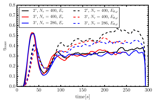
Figure 18.— Efficiency factors $\eta_{\mathrm{conv}}$ for the conversion of the total nuclear energy generation rate into turbulent energy in radial motions ($E_{r}$, solid lines) and non-radial motions ($E_{\theta},\varphi$, dashed lines) for the baseline run with an angular resolution of $3^{\circ}$ degrees and $N_{r}=400$ radial zones (black curves) and for two low-resolution runs with an angular resolution of $2^{\circ}$ and a radial resolution of 400 zones (red) and 286 zones (blue).

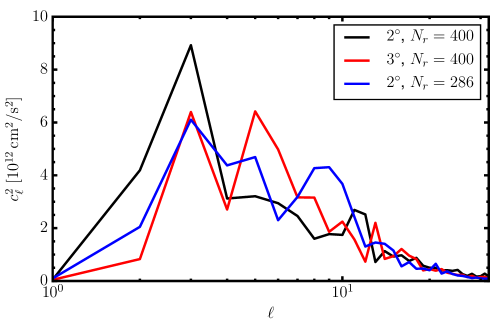
Figure 19.— Power $c_{\ell}^{2}$ in different multipoles $\ell$ for the decomposition of the radial velocity at $r=4000\,\mathrm{km}$ into spherical harmonics $Y_{\ell m}$ at a time of $210\,\mathrm{s}$ for the baseline run with an angular resolution of $3^{\circ}$ degrees and $N_{r}=400$ radial zones (black curve) and for two low-resolution runs with an angular resolution of $2^{\circ}$ and a radial resolution of 400 zones (red) and 286 zones (blue). Although the dominant angular wavenumbers are similar, the baseline run shows more power in $\ell=2$ and $\ell=3$ modes.

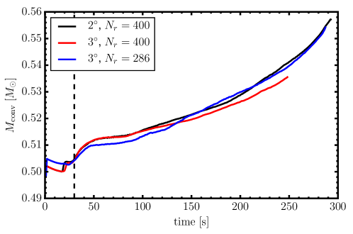
Figure 20.— Growth of the mass $M_{\mathrm{conv}}$ of the oxygen shell as a function of time for the baseline run with an angular resolution of $3^{\circ}$ degrees and $N_{r}=400$ radial zones (black curve) and for two low-resolution runs with an angular resolution of $2^{\circ}$ and a radial resolution of 400 zones (red) and 286 zones (blue). Note that $M_{\mathrm{conv}}$ starts at a slightly different value in the run with $N_{r}=286$ because the initial model is mapped to a different grid than for $N_{r}=400$.

Appendix B Effects of Resolution and Stochasticity

Limited resolution is always a cause of concern for turbulent flow as in convective shell burning. Current models of shell burning during the final stages like Couch et al. (2015) and ours are limited to $\mathord{\sim}1.5$ million zones to cover the region of interest, and a significant increase in resolution is currently not affordable. To gauge potential resolution effects, we have, however, computed two additional runs with lower resolution, and compare key quantities of those models to the baseline run. We both consider the case of a reduced angular resolution of $3^{\circ}$ with the same radial grid as well as a simulation with a resolution of $3^{\circ}$ and a coarser radial grid of 286 zones (with $\Delta r/r=1\%$).

The two complementary low-resolution simulations also help to address another important effect to a limited extent, i.e. stochastic variations in the convective flow geometry. With just three different models computed at different resolutions, it is obviously impossible to distinguish cleanly between the effects of resolution and stochasticity. The three models merely define a vague “band of uncertainty”, and only permit limited conclusions about the underlying cause for the variations between the models.

While all three models exhibit very similar nuclear energy generation rates, the dynamics of the convective flow is slightly different. Figure 7 compares the efficiency factor $\eta_{\mathrm{conv}}$ (Equation 14) for the conversion of nuclear energy into the components $E_{r}$ and $E_{\theta,\varphi}$ of the turbulent kinetic energy (which is essentially the same as comparing $E_{r}$ and $E_{\theta,\varphi}$ directly because of the extremely similar burning rate). $\eta_{\mathrm{conv}}$ does not differ substantially for the two low-resolution runs. Variations between the different simulations are typically on the level of $\mathord{10}\%$ or less, i.e. of the same order as the stochastic fluctuations within each run, and there is thus no clear evidence for a strong resolution dependence. This in line with findings from a different context (convection in core-collapse supernova explosions), where Handy et al. (2014) and Radice et al. (2016) found that the global energetics of the flow is well captured even with a modest resolution of $2\ldots 3^{\circ}$ in angle and $\mathord{\sim}100$ radial zones across the convective region.

The non-radial kinetic energies in the low-resolution runs differ more strongly from the baseline run, especially after $190\,\mathrm{s}$. It is not clear, however, whether this is a resolution effect or due to stochastic variations. The higher non-radial kinetic energy in the baseline run appears to be connected to a slightly different eddy geometry, which could suggest stochasticity rather than differences in resolution as the culprit for the differences between the runs. Figure 19 shows the coefficients $c_{\ell}^{2}$ for the decomposition of the radial velocity into spherical harmonics (computed according to Equation 30) at a time of $210\,\mathrm{s}$ and demonstrates a slightly stronger preponderance of low-$\ell$ modes in the baseline run compared to the low-resolution models. It is thus conceivable that the lateral flows from the updrafts to the downdrafts at the top and bottom of the convective shell must be slightly faster in the baseline run merely to ensure mass conservation in a flow that is (almost) anelastic: In the baseline run, the lateral flow must transport mass from the updrafts to the downdrafts (and vice versa a the bottom of the shell) at the same rate as in the low-resolution runs, but over a larger distance; hence the ratio of non-radial to radial turbulent velocities is larger.

Whatever the underlying cause, the lesson of our minimal resolution study is that we should anticipate uncertainties in the convective velocities, which scale with $\eta_{\mathrm{conv}}^{1/2}$, of $\mathord{\lesssim}10\%$, and that the dominant angular wavenumber of the convective eddies may also vary slightly.

Even the growth of the oxygen shell by entrainment is not too dissimilar for the three different runs as shown by Figure 20. Again it is unclear to what extent the variations in entrainment are stochastic or due to resolution effects. The resolution requirements for the problem at hand may be mitigated by the “softness” of the convective boundary: Interfacial waves develop on relatively large scales, so that the individual breaking billows are typically covered by $\mathord{\sim}10$ zones or more. This is still well below the resolution of almost 50 zones in the transition of the best-resolved global simulations of convective boundary mixing in the context of hydrogen ingestion (Herwig et al., 2014; Woodward et al., 2015), and hence more caution is in order concerning the convergence of the entrainment rate than for the convective velocities and eddy scales.

References

- Andreopoulos et al. (2000) Andreopoulos, Y., Agui, J. H., & Briassulis, G. 2000, Annual Review of Fluid Mechanics, 32, 309
- Arnett (1994) Arnett, D. 1994, ApJ, 427, 932
- Arnett et al. (2009) Arnett, D., Meakin, C., & Young, P. A. 2009, ApJ, 690, 1715, 0809.1625
- Arnett & Meakin (2011) Arnett, W. D., & Meakin, C. 2011, ApJ, 733, 78
- Arnett et al. (2015) Arnett, W. D., Meakin, C., Viallet, M., Campbell, S. W., Lattanzio, J. C., & Mocák, M. 2015, ApJ, 809, 30, 1503.00342
- Asida & Arnett (2000) Asida, S. M., & Arnett, D. 2000, ApJ, 545, 435
- Bazan & Arnett (1994) Bazan, G., & Arnett, D. 1994, ApJ, 433, L41
- Bazan & Arnett (1998) ——. 1998, ApJ, 496, 316
- Biermann (1932) Biermann, L. 1932, ZAp, 5, 117
- Böhm-Vitense (1958) Böhm-Vitense, E. 1958, ZAp, 46, 108
- Boris et al. (1992) Boris, J. P., Grinstein, F. F., Oran, E. S., & Kolbe, R. L. 1992, Fluid Dynamics Research, 10, 199
- Burrows & Goshy (1993) Burrows, A., & Goshy, J. 1993, ApJ, 416, L75+
- Burrows & Hayes (1996) Burrows, A., & Hayes, J. 1996, Physical Review Letters, 76, 352
- Chandrasekhar (1961) Chandrasekhar, S. 1961, Hydrodynamic and Hydromagnetic Stability (Oxford: Clarendon)
- Chatzopoulos et al. (2014) Chatzopoulos, E., Graziani, C., & Couch, S. M. 2014, ApJ, 795, 92
- Chieffi & Limongi (2013) Chieffi, A., & Limongi, M. 2013, ApJ, 764, 21
- Christensen-Dalsgaard et al. (1996) Christensen-Dalsgaard, J. et al. 1996, Science, 272, 1286
- Colella & Woodward (1984) Colella, P., & Woodward, P. R. 1984, J. Comp. Phys., 54, 174
- Couch (2013) Couch, S. M. 2013, ApJ, 775, 35, 1212.0010
- Couch et al. (2015) Couch, S. M., Chatzopoulos, E., Arnett, W. D., & Timmes, F. X. 2015, ApJ, 808, L21, 1503.02199
- Couch & Ott (2013) Couch, S. M., & Ott, C. D. 2013, ApJ, 778, L7
- Couch & Ott (2015) ——. 2015, ApJ, 799, 5, 1408.1399
- Demarque et al. (2008) Demarque, P., Guenther, D. B., Li, L. H., Mazumdar, A., & Straka, C. W. 2008, Ap&SS, 316, 31, 0710.4003
- Dolence et al. (2013) Dolence, J. C., Burrows, A., Murphy, J. W., & Nordhaus, J. 2013, ApJ, 765, 110
- Eggleton (1972) Eggleton, P. P. 1972, MNRAS, 156, 361
- Fernández et al. (2014) Fernández, R., Müller, B., Foglizzo, T., & Janka, H.-T. 2014, MNRAS, 440, 2763, 1310.0469
- Fernando (1991) Fernando, H. J. S. 1991, Annual Review of Fluid Mechanics, 23, 455
- Foglizzo et al. (2007) Foglizzo, T., Galletti, P., Scheck, L., & Janka, H.-T. 2007, ApJ, 654, 1006
- Foglizzo et al. (2006) Foglizzo, T., Scheck, L., & Janka, H.-T. 2006, ApJ, 652, 1436
- Fryer et al. (2004) Fryer, C. L., Holz, D. E., & Hughes, S. A. 2004, ApJ, 609, 288
- Fryxell et al. (1989) Fryxell, B. A., Müller, E., & Arnett, D. 1989, Max-Planck-Institut für Astrophysik, Preprint0, 449
- Fuller et al. (2015) Fuller, J., Cantiello, M., Lecoanet, D., & Quataert, E. 2015, ApJ, 810, 101, 1502.07779
- Goldreich et al. (1997) Goldreich, P., Lai, D., & Sahrling, M. 1997, in Unsolved Problems in Astrophysics, ed. J. N. Bahcall & J. P. Ostriker, 269–280
- Grinstein et al. (2007) Grinstein, F., Margolin, L., & Rider, W. 2007, Implicit Large Eddy Simulation - Computing Turbulent Fluid Dynamics (Cambridge University Press)
- Guilet & Foglizzo (2012) Guilet, J., & Foglizzo, T. 2012, MNRAS, 421, 546, 1112.1427
- Handy et al. (2014) Handy, T., Plewa, T., & Odrzywołek, A. 2014, ApJ, 783, 125, 1312.3658
- Hanke et al. (2012) Hanke, F., Marek, A., Müller, B., & Janka, H.-T. 2012, ApJ, 755, 138
- Heger et al. (2000) Heger, A., Langer, N., & Woosley, S. E. 2000, ApJ, 528, 368
- Heger & Woosley (2010) Heger, A., & Woosley, S. E. 2010, ApJ, 724, 341, 0803.3161
- Heger et al. (2005) Heger, A., Woosley, S. E., & Spruit, H. C. 2005, ApJ, 626, 350
- Herwig et al. (2014) Herwig, F., Woodward, P. R., Lin, P.-H., Knox, M., & Fryer, C. 2014, ApJ, 792, L3, 1310.4584
- Huete et al. (2012) Huete, C., Wouchuk, J. G., & Velikovich, A. L. 2012, Phys. Rev. E, 85, 026312
- Huete Ruiz de Lira (2010) Huete Ruiz de Lira, C. 2010, Physica Scripta Volume T, 142, 014022, 1006.1819
- Janka (2012) Janka, H.-T. 2012, Annual Review of Nuclear and Particle Science, 62, 407
- Janka et al. (2016) Janka, H.-T., Melson, T., & Summa, A. 2016, ArXiv e-prints, 1602.05576
- Jones et al. (2016) Jones, S., Andrassy, R., Sandalski, S., Davis, A., Woodward, P., & Herwig, F. 2016, ArXiv e-prints, 1605.03766
- Kageyama & Sato (2004) Kageyama, A., & Sato, T. 2004, Geochemistry, Geophysics, Geosystems, 5, n/a, q09005
- Kippenhahn & Weigert (1990) Kippenhahn, R., & Weigert, A. 1990, Stellar Structure and Evolution (Berlin: Springer)
- Kolmogorov (1941) Kolmogorov, A. 1941, Akademiia Nauk SSSR Doklady, 30, 301
- Kuhfuss (1986) Kuhfuss, R. 1986, A&A, 160, 116
- Kuhlen et al. (2003) Kuhlen, M., Woosley, W. E., & Glatzmaier, G. A. 2003, in Astronomical Society of the Pacific Conference Series, Vol. 293, 3D Stellar Evolution, ed. S. Turcotte, S. C. Keller, & R. M. Cavallo, 147
- Lai & Goldreich (2000) Lai, D., & Goldreich, P. 2000, ApJ, 535, 402
- Landau & Lifshitz (1959) Landau, L. D., & Lifshitz, E. M. 1959, Course of theoretical physics, Vol. VI, Fluid mechanics (Oxford: Pergamon Press)
- Langer et al. (1983) Langer, N., Fricke, K. J., & Sugimoto, D. 1983, A&A, 126, 207
- Malkus & Veronis (1958) Malkus, W. V. R., & Veronis, G. 1958, Journal of Fluid Mechanics, 4, 225
- Martyushev & Seleznev (2006) Martyushev, L. M., & Seleznev, V. D. 2006, Phys. Rep., 426, 1
- Meakin & Arnett (2006) Meakin, C. A., & Arnett, D. 2006, ApJ, 637, L53
- Meakin & Arnett (2007a) ——. 2007a, ApJ, 665, 690
- Meakin & Arnett (2007b) ——. 2007b, ApJ, 667, 448
- Melson (2013) Melson, T. 2013, Master’s thesis, Ludwig-Maximilians Universtiät München
- Melson et al. (2015) Melson, T., Janka, H.-T., & Marek, A. 2015, ApJ, 801, L24, 1501.01961
- Miczek et al. (2015) Miczek, F., Röpke, F. K., & Edelmann, P. V. F. 2015, A&A, 576, A50, 1409.8289
- Mocák et al. (2014) Mocák, M., Meakin, C., Viallet, M., & Arnett, D. 2014, ArXiv e-prints, 1401.5176
- Mocák et al. (2008) Mocák, M., Müller, E., Weiss, A., & Kifonidis, K. 2008, A&A, 490, 265, 0805.1355
- Mocák et al. (2009) ——. 2009, A&A, 501, 659, 0811.4083
- Müller et al. (2016) Müller, B., Heger, A., Liptai, D., & Cameron, J. B. 2016, MNRAS, 460, 742, 1602.05956
- Müller & Janka (2015) Müller, B., & Janka, H.-T. 2015, MNRAS, 448, 2141, 1409.4783
- Murphy & Burrows (2008) Murphy, J. W., & Burrows, A. 2008, ApJ, 688, 1159
- Murphy et al. (2004) Murphy, J. W., Burrows, A., & Heger, A. 2004, ApJ, 615, 460
- Murphy et al. (2013) Murphy, J. W., Dolence, J. C., & Burrows, A. 2013, ApJ, 771, 52, 1205.3491
- Murphy & Meakin (2011) Murphy, J. W., & Meakin, C. 2011, ApJ, 742, 74
- Paxton et al. (2011) Paxton, B., Bildsten, L., Dotter, A., Herwig, F., Lesaffre, P., & Timmes, F. 2011, ApJS, 192, 3, 1009.1622
- Paxton et al. (2013) Paxton, B. et al. 2013, ApJS, 208, 4, 1301.0319
- Peebles (1993) Peebles, P. J. E. 1993, Principles of Physical Cosmology
- Radice et al. (2016) Radice, D., Ott, C. D., Abdikamalov, E., Couch, S. M., Haas, R., & Schnetter, E. 2016, ApJ, 820, 76, 1510.05022
- Ribner (1987) Ribner, H. S. 1987, AIAA Journal, 25, 436
- Smith & Arnett (2014) Smith, N., & Arnett, W. D. 2014, ApJ, 785, 82, 1307.5035
- Stancliffe et al. (2011) Stancliffe, R. J., Dearborn, D. S. P., Lattanzio, J. C., Heap, S. A., & Campbell, S. W. 2011, ApJ, 742, 121, 1109.1289
- Strang & Fernando (2001) Strang, E. J., & Fernando, H. J. S. 2001, Journal of Fluid Mechanics, 428, 349
- Sukhbold & Woosley (2014) Sukhbold, T., & Woosley, S. E. 2014, ApJ, 783, 10, 1311.6546
- Summa et al. (2016) Summa, A., Hanke, F., Janka, H.-T., Melson, T., Marek, A., & Müller, B. 2016, ApJ, 825, 6, 1511.07871
- Takahashi & Yamada (2014) Takahashi, K., & Yamada, S. 2014, ApJ, 794, 162, 1408.3503
- Viallet et al. (2011) Viallet, M., Baraffe, I., & Walder, R. 2011, A&A, 531, A86, 1103.1524
- Viallet et al. (2016) Viallet, M., Goffrey, T., Baraffe, I., Folini, D., Geroux, C., Popov, M. V., Pratt, J., & Walder, R. 2016, A&A, 586, A153
- Viallet et al. (2013) Viallet, M., Meakin, C., Arnett, D., & Mocák, M. 2013, ApJ, 769, 1, 1212.6365
- Weaver et al. (1978) Weaver, T. A., Zimmerman, G. B., & Woosley, S. E. 1978, ApJ, 225, 1021
- Wongwathanarat et al. (2010) Wongwathanarat, A., Hammer, N. J., & Müller, E. 2010, A&A, 514, A48, 1003.1633
- Woodward et al. (2015) Woodward, P. R., Herwig, F., & Lin, P.-H. 2015, ApJ, 798, 49
- Woosley et al. (2002) Woosley, S. E., Heger, A., & Weaver, T. A. 2002, Rev. Mod. Phys., 74, 1015
- Woosley & Weaver (1988) Woosley, S. E., & Weaver, T. A. 1988, Phys. Rep., 163, 79
- Woosley et al. (2004) Woosley, S. E., Wunsch, S., & Kuhlen, M. 2004, ApJ, 607, 921, astro-ph/0307565
- Wouchuk et al. (2009) Wouchuk, J. G., Huete Ruiz de Lira, C., & Velikovich, A. L. 2009, Phys. Rev. E, 79, 066315
- Wuchterl & Feuchtinger (1998) Wuchterl, G., & Feuchtinger, M. U. 1998, A&A, 340, 419