Arctic curves of the six-vertex model
on generic domains: the Tangent Method

Abstract.

We revisit the problem of determining the Arctic curve in the six-vertex model with domain wall boundary conditions. We describe an alternative method, by which we recover the previously conjectured analytic expression in the square domain. We adapt the method to work for a large class of domains, and for other models exhibiting limit shape phenomena. We study in detail some examples, and derive, in particular, the Arctic curve of the six-vertex model in a triangoloid domain at the ice-point.

1. Introduction

Statistical mechanics models in two dimensions with a discrete symmetry group, within a pure phase, usually show a spatially-homogeneous order parameter and independence from the boundary conditions [DG-72]. This can be understood by simple entropic arguments on local excitations. The prototype example is the Ising Model, where the broken symmetry group is just $\mathbb{Z}_{2}$.

Nonetheless, certain models, characterised by the presence of conservation laws, under particular conditions may break this paradigm and show phase-separation phenomena and the emergence of a limit shape [KO-05, RP-10]. In this case we may have spatial dependence of the order parameter, a strong dependence from the boundary conditions, and even frozen regions, in which the local entropy vanishes. This is now possible because the conservation law forbids local excitations on frozen-region vacua, the smallest perturbations taking the form of a directed path which, in each direction, shall either reach the boundary, or a non-frozen (liquid) region. The interface between frozen and liquid regions, for a given model in a given domain, is called Arctic curve. The challenge of its determination is the subject of the present paper.

Among the models presenting phase separation and limit shape phenomena, those amenable to discrete free fermions are the most widely studied. Early examples include Young diagrams with the Plancherel measure [KV-77], the evaporation of a cubic crystal [NienhuisCrystal, CK-01, FS-03], domino tilings of the Aztec diamond, [JPS-98], boxed plane partitions [CLP-98], Schur processes [OR-01]. These examples may all be viewed as dimer models on planar bipartite graphs, for which a general theory has been constructed [KO-06, KO-05, KOS-06]; other approaches exist for certain subclasses of models [CJ-14, Pet-14, BK-16, BBCCR-15]. An interesting connection between limit shape phenomena in such models and the out-of-equilibrium evolution of one-dimensional quantum free-fermion models has been recently unveiled [ADSV-15].

Other free-fermionic models presenting a similar phenomenology are defined in terms of iterated transformations applied to a deterministic initial configuration. Examples of such models include ‘groves’ on the triangle [CSpeyer-04, PSpeyer-05] (see also [BdTK-15] for promising results on the ‘massive deformation’), and double-dimer configurations on ‘cubic-corner graphs’ [KP-16]. Some models are in both families, for example domino tilings also arise from the octahedron relation of cluster algebras [Spe07, Y-09, DiFSG14]

Another important instance for phase separation and limit shape phenomena is the six-vertex model [E-99, Zj-02, RP-10, RS-15, CGP-15], with various choice of fixed boundary conditions, among which the domain-wall boundary conditions [K-82] play a preeminent role. The model can be viewed as a nontrivial (‘interacting’, yet exactly solvable [L-67a, B-82]) generalization of the domino tilings of some domain in the square lattice [EKLP-92]. In this context, limit shape phenomena still need further understanding, although some progress has been made [BCG-16, BP-16] for the ‘stochastic’ version of the model [GS-92].

For interacting models out of free-fermionic or stochastic special points, very few exact results are available on these phenomena. The evaluation of the free energy of the six-vertex model with domain-wall boundary conditions [KZj-00, Zj-00, BL-13] provided the first quantitative indication of phase separation in the model. The sole other result in this context concerns (a strongly supported conjecture for) the analytic expression for the Arctic curve of the six-vertex model on a square region of the square lattice, with domain wall boundary conditions [CP-07b, CP-07a, CP-08, CP-09, CPZj-10]. The derivation is based on the study of an observable, the emptiness formation probability (EFP), so, for short, we can call this the EFP Method. This result, reviewed in Section 2, shows a much richer phenomenology w.r.t. dimers, and more generally, free-fermionic models: most notably the curve is algebraic if and only if the parameters of the model are tuned to a so-called root of unity case, and it is non-analytic at the points of contact with the boundary of the domain [CPN-11]. This is at variance with free-fermionic models, where the curve is algebraic, and, even when non-connected, different connected components arise naturally as different branches of the same curve [KO-05]. Because of this rich phenomenology, and with the aim of understanding phase-separation phenomena in the presence of an interaction, extension of these results to a larger class of domains is of great interest.

The present paper provides an alternative approach to the EFP Method, that we call Tangent Method. It is based on a detailed analysis of the line-type fundamental excitations of the frozen regions. In a sense, it gives a ‘geometric interpretation’ to the analytic results arising from the EFP Method, which surprisingly had shown that the Arctic curve is the caustic of a family of lines determined by a single one-point boundary observable; this is here understood as the fact that basic excitations form random walks from a given boundary point to the Arctic curve, which are almost-straight in the thermodynamic limit, and reach the curve tangentially, from which the name of the method.

In this paper we use the Tangent Method to rederive the conjectured formula for the Arctic curve in the square domain, for generic parameters of the six-vertex models (Section 3). By the same method, we determine the analytic expression for the Arctic curve of the six-vertex model at its ice point, in a triangoloid domain, constructed out of the crossing of three bundles of spectral lines, that has two independent aspect-ratio parameters (Section 5). We also provide a relation between the Arctic curve and the generating function of the one-point boundary correlation function, that holds for a large class of domains, and generic values of the parameters of the model (Section 4).

As an instructive ‘minimal working example’ of our method, we also provide a very short derivation of the Arctic Ellipse for lozenge tilings of the $a\times b\times c$ hexagon (MacMahon boxed plane partitions), which is self-contained except for the use of the Gelfand–Tsetlin formula [GT-50], thus reproducing the classical result in [CLP-98] (Appendix C).

2. The Arctic curve in the square: known facts

2.1. The six-vertex model

The six-vertex model is an exactly solvable model of equilibrium statistical mechanics [L-67a, B-82]. In its simplest realisation, it is just defined on a portion of the square grid. In its most general ‘integrable’ realisation, it is defined on a planar graph, with all vertices of degree 4 and 1, obtained from the intersection (in generic position) of a collection of open and/or closed curves in the plane [BaxPP].

An intermediate family of domains consists of the framework of [BaxPP], in which we have a finite number of bundles $\alpha$ of parallel lines, pairwise mutually crossing, where the number $n_{\alpha}$ of lines per bundle goes to infinity in the thermodynamic limit. In this case the lattice consists of a finite number of rectangular portions of the square lattice, glued together along some of their boundaries.

We will consider here the most basic example of such a geometry, the crossing of two bundles, and, in Section 5, the second simplest realisation, consisting of three bundles. In this introduction, for sake of simplicity, we will define the model only in the simplest case, the rectangular $N\times M$ geometry.

We have thus $NM$ vertices of degree 4, $2(N+M)$ vertices of degree 1 (external vertices), $(N+1)M$ horizontal and $N(M+1)$ vertical edges, of which overall $2(N+M)$ are external edges, i.e. are incident on an external vertex. All other edges will be called internal. A vertex which is first-neighbour to an external vertex will be called a boundary vertex (we have $2N+2M-4$ such vertices). An internal edge incident to a boundary vertex will be called a boundary edge. We label the internal vertices with the coordinates $(r,s)$, $r\in\{1,\dots,N\}$, $s\in\{1,\dots,M\}$, in the obvious way. Edges will be labeled by the coordinates of their midpoint.

The states of the model are configurations of arrows on the edges of the lattice, i.e. orientations of the graph, satisfying the ice rule at all internal vertices, namely, there are two incoming and two outgoing arrows. This rule selects six possible local configurations around a vertex, to which we give names as in Fig. 1.

An equivalent and also graphically appealing description of the configurations of the model can be given by drawing a thick edge whenever an arrow is down or left, and a thin edge otherwise. Due to the ice-rule, the thick edges form directed paths, which may be oriented in such a way that all the steps are north and east. In particular, all these paths are open and reach the boundary of the domain. The states of the model can thus be depicted as configurations of paths satisfying the rules shown in Fig. 1. From now on we shall mainly refer to the path picture. Our notations are consistent with [B-82, Sec. 8.3].

Figure 1. The six possible types of vertex configurations in terms of arrows (top), or of paths (bottom), and their Boltzmann weights.

The model is further specified by assigning a Boltzmann weight $w_{i}$, $i\in\{1,\dots,6\}$, to each vertex configuration, as in Fig. 1. The Boltzmann weight of a given arrow configuration $\sigma$ is the product over internal vertices of the corresponding weight, which can be written as

$$w(\sigma)=\prod_{i=1}^{6}w_{i}^{n_{i}(\sigma)},$$ (2.1)

where it is understood that $n_{i}(\sigma)$ is the number of vertices of type $i$ in $\sigma$. The obvious constraint $\sum_{i}n_{i}(\sigma)=NM$ shows that one such parameter is redundant.

2.2. Fixed boundary conditions

Each of the external vertices may have an incoming or an outgoing arrow. If specified in advance, we say that we have fixed boundary conditions, otherwise we have free boundary conditions. Of course, a fixed boundary condition, for having any valid configuration, requires that the overall number of incoming and of outgoing arrows are equal. This constraint has a counterpart in path representation: we must have as many thick edges on the south and west sides altogether as on the north and east sides altogether.

Another useful property of fixed boundary conditions in a rectangular geometry is that we know in advance how many horizontal and vertical thick edges there are in the system. Furthermore, a directed path going (say) from the south to the north sides makes as many left-turns as right-turns, while one going (say) from west to north makes one more left turn. Thus, we also know in advance the difference between the total number of left- and right-turns. This gives control on the three linear combinations $n_{5}-n_{6}$, $2n_{2}+2n_{4}+n_{5}+n_{6}$ and $2n_{2}+2n_{3}+n_{5}+n_{6}$. , which, together with the forementioned $n_{1}+\cdots+n_{6}=NM$, makes only two independent parameters out of the six weights $w_{1}$, …, $w_{6}$.

For this reason, in the case of fixed boundary conditions, up to multiplying the partition function by a trivial factor, symmetry of the Boltzmann weights under reversal of arrows can be imposed with no loss of generality, and it is customary to introduce the three parameters

$$\mathsf{a} :=w_{1}=w_{2}, \mathsf{b} :=w_{3}=w_{4}, \mathsf{c} :=w_{5}=w_{6},$$ (2.2)

and also the convenient parameterization

$$\Delta =\frac{\mathsf{a}^{2}+\mathsf{b}^{2}-\mathsf{c}^{2}}{2\mathsf{a}\mathsf{b}}, t =\frac{\mathsf{b}}{\mathsf{a}}.$$ (2.3)

The probabilistic space of parameters, i.e. the one for which the Boltzmann weight $w(\sigma)$ is real positive for all configurations, is for $\mathsf{a},\mathsf{b},\mathsf{c}\in\mathbb{R}^{+}$, and thus corresponds to $t\in\mathbb{R}^{+}$ and $\Delta<\frac{1}{2}(t+\frac{1}{t})$.

In the phase separation phenomena we will see the emergence of four types of frozen patterns, using vertices $w_{1}$, …, $w_{4}$. These patterns can be selected on the whole domain by taking homogeneous choices on the four sides. Their smallest perturbation, e.g. having exactly two thick edges, gives the simple problem of enumerating configurations consisting of a single directed lattice path (discussed in Appendix A). Trivial as it may seem, when combined with the more remarkable facts coming from the full-fledged six-vertex model, this setting will prove of some use in our treatment.

Up to symmetry, we have a unique further choice of homogeneous fixed boundary conditions, namely, in the case $N=M$, of having thick edges on north and west sides, and thin edges on south and east sides. In this case the geometry allows many configurations, and the paths, which start on the west and arrive on the north being maximally packed, travel in a rainbow fashion in the bulk, with a positive amount of entropy. This setting is called domain-wall boundary conditions (DWBC) [K-82], see Figure 2, left.

2.3. Gibbs measure and correlation functions

We now assume some fixed boundary conditions $\sigma_{B}$ have been imposed on the boundary $\partial\Lambda$ of a domain $\Lambda$. The partition function is the sum over the set of configurations of the model which are compatible with the given boundary conditions, each state being assigned its Boltzmann weight $w(\sigma)$ as in (2.1)

$$Z_{\Lambda}(\sigma_{B})=\sum_{\sigma\;:\;\sigma|_{\partial\Lambda}=\sigma_{B}}w(\sigma).$$ (2.4)

Correspondingly, $w(\sigma)/Z_{\Lambda}(\sigma_{B})$ is the Gibbs measure on the states of the model with given boundary conditions.

For each edge $e$ of the lattice we define the characteristic function:

$$\chi_{e}(\sigma):=\left\{\begin{array}[]{l}1,\quad\mathrm{if\ }e\mathrm{\ is\ thick},\\ 0,\quad\mathrm{if\ }e\mathrm{\ is\ thin},\end{array}\right.$$ (2.5)

The expectation value of a product of these observables with respect to the Gibbs measure,

$$\langle\chi_{e_{1}},\dots,\chi_{e_{n}}\rangle_{\sigma_{B}}:=\frac{1}{Z_{\Lambda}(\sigma_{B})}\sum_{\sigma\;:\;\sigma|_{\partial\Lambda}=\sigma_{B}}w(\sigma)\prod_{j=1}^{n}\chi_{e_{j}}(\sigma),$$ (2.6)

is called an edge correlation function. These correlation functions clearly form a complete linear basis. A boundary correlation function is a correlation function involving only boundary edges.

2.4. Phases of the model, and particular cases

The study of the thermodynamic limit of the model with periodic boundary conditions shows the emergence of three physical regimes, or phases, according to the value of the parameter $\Delta$, namely ferroelectric ($\Delta>1$), anti-ferroelectric ($\Delta<-1$), and disordered, or critical ($|\Delta|<1$), see [B-82] for details. In the context of phase separation phenomena, the three phases are sometimes called solid, gaseous, and liquid, respectively. Some of this phenomenology survives in situations showing phase separation, see [RP-10] for details.

As anticipated, the special case $\Delta=0$ is related to free fermions on a lattice. In particular, at $t=1$, there is a correspondence with non-intersecting lattice paths, dimer models and domino tilings, the most notorious example being the so-called domino tilings of the Aztec Diamond [EKLP-92]. In the light of such correspondence, the model with generic value of $\Delta$ can be viewed as one of interacting dimers. Values $t\not=1$ correspond to the presence of a non-vanishing external field (called ‘bias’ in [JPS-98]), that favours one of the two possible orientations of the dimers.

Another case of interest, in particular for its relations with Algebraic Combinatorics, is the so-called ice point, where $\mathsf{a}=\mathsf{b}=\mathsf{c}$, and hence, $\Delta=1/2$ and $t=1$. In this case the configurations of the model with domain wall boundary conditions are in bijection with Alternating Sign Matrices [MRR-82, EKLP-92], see [pzjhdr] for details.

2.5. The one-point boundary correlation function

As a specialty of the domain-wall boundary conditions, the ice-rule strongly constrains the pattern of vertex configurations in the first/last row/column. For example, in the bottom-most row of vertical edges (besides the boundary ones) there must be exactly one thick edge, at some horizontal coordinate $1\leq r\leq N$. We call this value (south) refinement position.

We will call $H_{N}^{(r)}$ the probability that the refinement position is $r$, i.e., formally,

$$H_{N}^{(r)}:=\langle\chi_{e_{(r+1,3/2)}}\rangle.$$ (2.7)

These quantities are naturally collected in the corresponding generating function

$$h_{N}(z):=\sum_{r=1}^{N}H_{N}^{(r)}z^{r-1}=\langle\,\sum_{r=1}^{N}\chi_{e_{(r,3/2)}}z^{r-1}\,\rangle.$$ (2.8)

This correlation function was studied, in particular, in [BPZ-02], where it was also evaluated in the form of a determinant.

Figure 2. Left, a typical configuration of the six-vertex model with domain-wall boundary conditions, in path representation. Here $N=8$. Right: a configuration in the refined ensemble with $r=6$, i.e. this configuration contributes to the probability $H_{8}^{(6)}$.

The uniqueness of the refinement position is due to DWBC, but is not specially related to the square geometry, and holds in the more general case of multiple bundles of spectral lines discussed above, provided that the boundary conditions are uniform on the given side. Below, given a domain $\Lambda$ of this form, we shall use the notations $H_{\Lambda}^{(r)}$, $h_{\Lambda}(z)$ for the related one-point boundary correlation function, and for the corresponding generating function (this notation is somewhat elliptic, as it leaves understood the precise choice of DWBC and the reference side).

2.6. The thermodynamic limit

The Arctic curve and limit shape phenomena are of course effects of large volume. At most, the liquid region of a single configuration, taken with the Gibbs measure, is just almost surely of the shape given by the Arctic curve up to fluctuations, which are sub-linear (conjectured to be of order $N^{\frac{1}{3}}$, in analogy with exact results in the $\Delta=0$ case [J-00, J-05], although the precise value of this exponent, assuming that it is smaller than 1, is immaterial for the purposes of the present paper). Thus, we are led to spend a few words on how the thermodynamic limit is performed in presence of phase separation phenomena. We will also introduce a quantity, $r(z)$, which has the same information as $H_{N}^{(r)}$, but will be more adapted to our purposes.

For the square domain, we just perform a thermodynamic limit $N\to\infty$, and simultaneously rescale the lattice coordinates $(r,s)$, in the obvious way, i.e. $r=\lceil Nx\rceil$, $s=\lceil Ny\rceil$, and $(x,y)\in[0,1]^{2}$. We shall refer to this thermodynamic/continuum limit as scaling limit. In this limit, the Arctic curve is described by an equation of the form $C(x,y)=0$. As a matter of fact, except for the point $\Delta=0$, it is nowadays strongly believed that this curve is analytic only piecewise, in each arc interval between two points of contact with the boundary of the domain, thus in fact we have, in the square, four equations, one per corner, $C_{\rm SW}(x,y)=0$, and so on (for the quadruple SW, SE, NW, NE), and four expressions for the contact points, $(0,\kappa_{\rm W})$, $(\kappa_{\rm S},0)$ $(1,\kappa_{\rm E})$ and $(\kappa_{\rm N},0)$. Of course, the symmetry of the problem (up to sending $t\leftrightarrow t^{-1}$ where needed) relates the different arcs, and we can concentrate, say, on the south-east arc without loss of generality (see [CP-09] for more details).

If we call

$$S_{N}(x):=-\frac{1}{N}\ln H_{N}^{(\lfloor xN\rfloor)}$$ (2.9)

it is expected in general circumstances (and proven for the square domain [CP-09, CPZj-10]) that this function has a sensible limit, i.e. that $S(x)=\lim_{N\to\infty}S_{N}(x)$ exists, and is a convex smooth function, with a single minimum at some $0\leq\kappa\leq 1$ (the contact point of the curve on this side), where it is valued zero. In other words, the refinement position $r$ fluctuates around its typical value on a sub-linear range.

Similarly, the value of the function $h_{N}(z)$ is not quite interesting per se, while its derivative w.r.t. $z$, which allows to extract $S(x)$ by Legendre transform, is more relevant. This suggests to define

$$r(z):=\lim_{N\to\infty}\frac{1}{N}z\frac{\mathrm{d}}{\mathrm{d}z}\ln h_{N}(z),$$ (2.10)

(again this limit exists and is finite for the square domain, and it shall be in very general circumstances). Indeed, letting $r=\lceil\xi N\rceil$, with $0<\xi<1$, for large $N$ we may write:

$$h_{N}(z)\propto\int_{0}^{1}\mathrm{d}\xi H_{N}^{(\lceil\xi N\rceil)}\mathrm{e}^{\lceil\xi N\rceil\ln z}$$ (2.11)

where the proportionality constant is independent of $z$, and inessential for our purposes. Then, from the log-convexity of $H$, standard saddle-point arguments lead to

$$r(z):=\lim_{N\to\infty}\frac{1}{N}z\frac{\mathrm{d}}{\mathrm{d}z}\ln h_{N}(z)=\xi_{sp}$$ (2.12)

where $\xi_{sp}$ is the solution of the saddle-point equation

$$\frac{1}{N}\frac{\mathrm{d}\ }{\mathrm{d}\xi}\ln H_{N}^{(\lceil\xi N\rceil)}+\ln z=0.$$ (2.13)

This relation will turn out to be useful below.

In the situation in which we have several crossing bundles, each consisting of $n_{\alpha}$ lines, as we said this identifies a finite collection of rectangles. We may define $2N=\sum_{\alpha}n_{\alpha}$, use a local system of coordinates in each rectangle (or in each collection of rectangles that can be glued together without conical singularities), and rescale coordinates $(r,s)$ again in the obvious way, i.e., under the limit $N\to\infty$ with $\ell_{\alpha}:=n_{\alpha}/N$, we rescale the lattice coordinates $(r,s)$ as $r=\lceil Nx\rceil$, $s=\lceil Ny\rceil$, and $(x,y)\in[0,\ell_{\alpha}]\times[0,\ell_{\beta}]$ for the rectangle consisting of the crossing of bundles $\alpha$ and $\beta$.

2.7. The Arctic Curve Conjecture

In [CP-09], using what we called above ‘the EFP method’, it has been shown that the Arctic curve of the six-vertex model on the square domain with DWBC is completely determined by the boundary correlation function $H_{N}^{(r)}$, through the following relation:

Conjecture 2.1 (Arctic Curve Conjecture [CP-09]).

The south-east arc of the Arctic curve of the six-vertex model with domain wall boundary conditions can be expressed in parametric form $x=x(z)$, $y=y(z)$, with $z\in[1,+\infty)$, as the solution of the linear system of equations

$$F(x,y;z) =0, \frac{\mathrm{d}}{\mathrm{d}z}F(x,y;z) =0,$$ (2.14)

with

$$F(x,y;z)=x-\frac{z(t^{2}-2\Delta t+1)}{(z-1)(t^{2}z-2\Delta t+1)}y-r(z).$$ (2.15)

Note the change of coordinates $x\to 1-x$, with respect to [CP-09]. The quantity $r(z)$ is defined as in (2.10), in terms of $h_{N}(z)=h_{N}(z;\Delta,t)$, the generating function (2.8). It has a complicated (but known [CP-09, CPZj-10]) expression for generic $\Delta$ and $t$, which however simplifies considerably at the free-fermion point $\Delta=0$ (domino tilings) and at the ‘combinatorial point’ $(\Delta,t)=(\frac{1}{2},1)$ (alternating-sign matrices):

$$\Delta=0\; : F(x,y;z) =x-\frac{z}{z-1}\frac{t^{2}+1}{t^{2}z+1}y-\frac{t^{2}z}{t^{2}z+1}$$ (2.16)

$$(\Delta,t)=({\textstyle\frac{1}{2}},1)\; : F(x,y;z) =x-\frac{1}{z-1}y-\frac{\sqrt{z^{2}-z+1}-1}{z-1}$$ (2.17)

We recall that by construction the solution of (2.14) provides only one of the four portions of the Arctic curve, between two consecutive contact points, i.e., points where the Arctic curve is tangent to the boundary of the square. Here we have focused on the lower-right arc, limited by the two contact points $(1-\kappa,0)$ and $(1,\kappa)$, corresponding to $z=1$ and $z\to\infty$, respectively. In particular we have

$$1-\kappa=r(1)=\lim_{N\to\infty}\left.\frac{1}{N}z\frac{\mathrm{d}}{\mathrm{d}z}\ln h_{N}(z)\right|_{z=1}.$$ (2.18)

The main steps in the derivation of the result above can be summarized as follows.

First, a specific correlation function, the emptiness formation probability (EFP), devised to detect spatial transition from order to disorder, is introduced. This quantity, evaluated at the coordinate $(r,s)$ on the $N\times N$ lattice, is the probability that all the lattice sites $(r^{\prime},s^{\prime})$ with $r^{\prime}\geq r$ and $s^{\prime}\leq s$ are occupied by a $w_{1}$ vertex. Remarkably, this quantity admits an exact formula in terms of some multiple integral representation [CP-07b].

Next, one has to study the asymptotic behaviour of this integral representation in the scaling limit, in the framework of the saddle-point approximation. In doing so, heuristic considerations suggest to formulate a strongly supported, but still unproven assumption that the spatial transition from order to disorder, and hence the Arctic curve, are characterized by the condensation of almost all roots of the saddle-point equation at the same known value. This assumption leads directly to the Arctic Curve Conjecture [CP-07a, CP-09].

Besides the relation between the curve and the boundary correlation function $r(z)$, the actual determination of the expression of the Arctic curve requires the explicit knowledge of the function $r(z)$, and the evaluation of its behaviour in the scaling limit [CP-09, CPZj-10].

It is worth emphasizing that, according to the conjecture above, the form of the Arctic curve inside the domain is completely determined in terms of a boundary quantity, namely the one-point boundary correlation function. At this stage of the reasoning, however, there appears no clear motivation for such a relation. Our alternative approach also addresses this point.

3. An alternative derivation of the Arctic Curve Conjecture

3.1. Preliminaries

To start with, let us investigate more closely in which functional form the one-point boundary correlation function determines the Arctic curve. It is useful to recall first some elementary geometry (see e.g. [librocurve]).

Let $\{\mathcal{C}_{z}\}_{z\in I}$ be a family of curves, in the $(x,y)$-plane, determined by a continuous parameter $z$ valued in a real interval $I$. The envelope $\mathcal{E}$ of the family is the (minimal) curve that is tangent to every curve of the family.

If the equation of the family $\{\mathcal{C}_{z}\}$ is given in Cartesian coordinates by $U(x,y;z)=0$, the non-singular points $(x,y)$ of the envelope $\mathcal{E}$ are the solutions of the system of equations

$$U(x,y;z) =0; \frac{{\rm d}}{{\rm d}z}U(x,y;z) =0.$$ (3.1)

By analogy with caustics in geometric optics, we call geometric caustic the envelope of a family of straight lines. In this case $U$ is of degree 1 in $x$ and $y$. This allows us to recognise the statement of the Arctic Curve Conjecture in a compact form: the portion of the Arctic curve is the geometric caustic of the family of lines in the $(x,y)$-plane,

$$U(x,y;z)=x-\frac{z(t^{2}-2\Delta t+1)}{(z-1)(t^{2}z-2\Delta t+1)}y-r(z)$$ (3.2)

for $z$ valued in the interval $[1,+\infty)$. Note that the slope of the lines, which is

$$\frac{z-1}{z}\left(1+\frac{t^{2}}{t^{2}-2\Delta t+1}(z-1)\right)$$

is indeed a monotone function from $[1,+\infty)$ to $[0,+\infty)$, provided that $\Delta<\frac{1}{2}(t+\frac{1}{t})$, as is in fact implied by the requirement of being in the probabilistic regime (i.e., $\mathsf{a},\mathsf{b},\mathsf{c}\in\mathbb{R}^{+}$).

This alternative formulation of the Arctic Curve Conjecture provides a elementary geometric construction, and thus suggests the existence of a simple ‘geometric principle’ underlying the relation between the Arctic curve and the boundary correlation function.

As we will explicitate in the remaining of the section, this principle is the fact that an isolated path in a system of interacting non-intersecting lattice paths is not sensible to the parameter $\Delta$, thus its trajectory is locally a lattice directed random walk, with some drift parameter fixed by the knowledge of its endpoints. And, in the scaling limit and at leading order, directed paths become straight lines. This is not unusual, as it corresponds to the mechanism by which deterministic trajectories emerge in the semi-classical limit of quantum theories in path-integral formulation.

3.2. The Tangency Assumption

The quantities $H_{N}^{(r)}$ have been introduced as probabilities in the model on the $N\times N$ domain, with partition function $Z_{N}$. On the other side, in light of their ‘boundary’ character, the related quantities $H_{N}^{(r)}Z_{N}/(\mathsf{a}^{N-r}\mathsf{c}\mathsf{b}^{r-1})$ can equally well be seen as the partition function of a model on the $(N-1)\times N$ rectangle, with DWBC up to one exception: on the south side there is one thick edge, at position $r$ (see Figure 2, and Figure 3 for a large example).

Yet again, the thick paths form a sort of rainbow, from their fixed incoming positions on the south- and west-sides, to their outgoing positions on the north-side. However this time, at difference with the $N\times N$ case, in general they do not all start and arrive densely packed. Two cases, depending from $r/N\lessgtr\kappa_{\rm S}$, occur, and we shall concentrate on the case $r/N>\kappa_{\rm S}$. Now the $N$th path, i.e. the only path starting from the south side, almost surely enters the south-east frozen region, in which thick edges are absent, and thus locally makes a directed random walk, with some drift parameter that remains constant for a while. This behaviour stops at the point in which the constraint of reaching the north-east corner enters in conflict with the edge-disjointness of the thick paths, and the presence of the liquid region inside the Arctic curve. At this point something else must happen. Heuristically, we expect the path to bent, and roughly follow the profile of the Arctic curve, up to the west contact point, and then go straight, in a frozen way, up to its final destination endpoint.

From this heuristic scenario we are led to formulate an ‘assumption’, whose aim is to divide the Tangent Method in two parts. On one side, the precise framework of the assumption provides a set of conditions to be verified, potentially on a case-analysis to be adapted from one system to another. On the other side, it provides a solid basis to establish once and for all the rigorous (but calculatory) part of the method, which, given the assumption, draws conclusions on the relationship between the Arctic curve and the function $r(z)$.

Assumption 3.1 (Tangency Assumption).

Consider the six-vertex model on the $(N-1)\times N$ domain, with DWBC except for the $r$th south boundary vertical edge being thick. In a suitable scaling limit, the resulting Arctic curve consists in the usual Arctic curve of the six-vertex model with domain wall boundary conditions, plus a straight segment, tangent to the bottom right portion of the Artic curve, and crossing the south boundary at $(r/N,0)$.

Numerical simulations strongly support the validity of this assumption in a variety of situations, see e.g., for the ice point $\mathsf{a}=\mathsf{b}=\mathsf{c}$, Fig. 3 and the right part of Fig. 5.

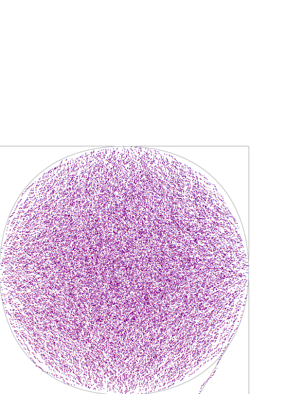
Figure 3. A typical configuration of the six-vertex model, on a rectangular domain of size $500\times 499$, and refinement position $r=400$ on the south side. This configuration is exactly sampled, at the ice point, $\mathsf{a}=\mathsf{b}=\mathsf{c}=1$. Blue and red dots correspond to $w_{5}$ and $w_{6}$ vertex configurations, respectively. In overlay in gray, the analytical prediction from the Tangent Assumption.

In the remaining of this section we shall summarise, somewhat in a sketchy way, why this assumption is sounding, and which steps one should perform in order to prove it rigorously.

• Let us call $p=(x,y)$ the coordinate at which the $N$th path, starting at position $(r,0)$, first reaches a location at a distance $\mathcal{O}(N^{\frac{1}{2}})$ from the $(N-1)$th thick path. Then, the $N$th path, in its portion from $(r,0)$ to $(x,y)$, is almost surely a random (corner-weighted) directed lattice path, in the pertinent ensemble (as illustrated in Appendix A). As such, in a large $N$ limit, it becomes a straight segment. This claim is completely under control.

• Let us consider the configurations of the other $N-1$ paths, which determine a (rescaled) liquid region $R\subset[0,1]^{2}$. First of all, this region is expected to be almost-surely convex after a coarse-graining of short-scale fluctuations (this shall be not hard to prove). Then, conditioning on the shape $R$, the position $(x,y)$ is such that the segment from $(r,0)$ to $(x,y)$ is tangent to $R$, with $p$ being the tangency point. This is the crucial observation. If true, it must originate from the fact that deviations of order $N$ from the tangent trajectory, on both sides, would decrease the free energy. This behaviour is well under control provided that the interacting non-intersecting lattice paths ensemble has a repulsive interaction in the frozen region of interest, which happens for $\mathsf{a}/\mathsf{c}\leq 1$, i.e. $\Delta\leq t/2$. It is conceivable, though, that the Tangent Method, suitably adapted, may be applied in the full probabilistic region of parameters, $\mathsf{a},\mathsf{b},\mathsf{c}\in\mathbb{R}^{+}$.

• The region $R$ concentrates, i.e., it has almost surely a given deterministic shape at leading order. This shall follow from the unicity of the associated variational problem, and thus from mild conditions on the form of the surface tension of the six-vertex model [RS-15].

• The deterministic limit of the region $R$ is the same of the limit of the liquid region in the $N\times N$ domain. This is again expected, but (in our perspective) hard to formalise. Indeed, we have essentially peeled away part of one thick path from the liquid region. This makes, by itself, less volume within the region (but only for a sub-linear thickness), but more volume available to the other $N-1$ paths for drifting towards south-east, due to the removal of non-crossing constraints (though, less volume available than what would be at disposal if we peeled off the full path, i.e. in the $(N-1)\times(N-1)$ square geometry, and we know that the limit shape has a thermodynamic limit). So the variation in the shape of $R$ is the difference of two effects, both sublinear, and as thus shall be sublinear.

3.3. The domain aaali

Let us now consider yet another geometry, namely, the $N\times(N+L)$ rectangular domain, for some non-negative $L$. Let us fix the axis origin so that the four corner vertices are located at $(1,N-1)$, $(1,-L)$, $(N,N-1)$, $(N,-L)$. We consider the following fixed boundary conditions: the north side has all thick edges, east and south sides have thin edges, the west side has thick its top-most $N-1$ edges, as well as its bottom-most, all other edges being thin. We denote this domain, with this choice of fixed boundary conditions, as $\Lambda_{N,L}$.

In this case, the Tangent assumption is rephrased as follows.

Assumption 3.2.

Consider the six-vertex model on the domain $\Lambda_{N,L}$. In the scaling limit, the Arctic curve consists in the usual Arctic curve of the six-vertex model with domain wall boundary condition, plus a straight segment, tangent to the bottom-right portion of the Artic curve, and reaching the south-west corner.

Indeed, the only further step from the Assumption 3.1 to 3.2 is that the straight line does not make an angle when crossing the $N$th row, which is rather obvious from entropic reasonings, given that the local weights are the same in the regions above and below, and the thick path is locally far away from other thick edges in that region.

Under Assumption 3.2, as we vary $L\in\mathbb{N}_{0}$, in the scaling limit we obtain a family of lines in the parameter $u=L/N$, with $u\in[0,\infty)$, that are all tangent to the bottom-right portion of the Arctic curve. For any fixed value of $u$, the corresponding line crosses the vertical axis at $(0,-u)$, and the horizontal axis at some random point $(\xi,0)$, where the behaviour of the random variable $\xi=r/N$ is discussed in a moment. We anticipate that this variable concentrates, so that the equation of this family of lines in the $(x,y)$-plane is

$$x-\frac{\xi(u)}{u}y-\xi(u)=0,$$ (3.3)

As we show below, for a certain $u=u(z)$, this is the family of lines appearing in the geometric formulation of the Arctic Curve Conjecture, equation (3.2).

3.4. Partition function of the six-vertex model on aaali

As a matter of fact, once one has control on $Z_{N}$ and $H_{N}^{(r)}$, evaluating the partition function of the model on the domain $\Lambda_{N,L}$ is a rather easy task. For this purpose we divide the domain $\Lambda_{N,L}$ into two portions, an upper domain $\Lambda_{N,L}^{(+)}$, containing the top-most $N-1$ rows of vertices, and a lower domain $\Lambda_{N,L}^{(-)}$, containing the remaining $L+1$ rows.

For every configuration there exists one path crossing the boundary between the two sub-domains, this occurring at some (random) horizontal coordinate $k$. Then, the sub-domain $\Lambda_{N,L}^{(+)}$, conditioned to this value $k$, is exactly of the form described at the beginning of Section 3.2, and thus has partition function

$$Z^{(+)}_{N,k} :=\frac{1}{\mathsf{a}^{N-k}\mathsf{b}^{k-1}\mathsf{c}}Z_{N}H_{N}^{(k)}=\frac{1}{\mathsf{a}^{N}}\frac{1}{t^{k-1}(t^{2}-2\Delta t+1)^{1/2}}Z_{N}H_{N}^{(k)}.$$ (3.4)

For the sub-domain $\Lambda_{N,L}^{(-)}$ that’s even simpler. The boundary conditions have all thin edges, except for one thick edge, $k$th from the left, on the north side, and one thick edge, the bottom-most, on the west side. Thus we are in the situation of a single oriented lattice path, for which the (easy) formulas are reminded in Appendix A in terms of the weight factors for going straight or making a left/right turn. The Boltzmann weights of the six-vertex model, see Fig. 1, induce a factor $\mathsf{b}/\mathsf{a}$ for each straight, and $\mathsf{c}/\mathsf{a}$ for each turn. The evaluation of the weighted enumeration of directed lattice paths in the $y\times x$ box, a classical result in combinatorics, is reported in equation (A.8). When expressed in terms of the quantities $\Delta$, $t$, see (2.3), this formula reads

$$P_{\Delta,t}(x,y)=t^{x+y+1}\sum_{l\geq 0}\binom{x}{l}\binom{y}{l}\left(\frac{t^{2}-2\Delta t+1}{t^{2}}\right)^{l+1/2}.$$ (3.5)

Thus, for the partition function of the six-vertex model on the lower domain, we may write:

$$Z^{(-)}_{N,L,k}=\mathsf{a}^{N(L+1)}P_{\Delta,t}(k-1,L)$$ (3.6)

The full partition function of the domain is then easily determined from the combination of (3.4) and (3.6)

In conclusion the partition function of the six-vertex model on the domain $\Lambda_{N,L}$ can be expressed as

$$Z_{\Lambda_{N,L}} =\sum_{k=1}^{N}Z^{(+)}_{N,k}Z^{(-)}_{N,L,k}=\frac{\mathsf{a}^{NL}Z_{N}}{\sqrt{t^{2}-2\Delta t+1}}\sum_{k=1}^{N}t^{1-k}H_{N}^{(k)}P_{\Delta,t}(k-1,L)$$ (3.7)

$$=\mathsf{a}^{NL}Z_{N}\sum_{k=1}^{N}\sum_{l\geq 0}\binom{k-1}{l}\binom{L}{l}t^{L-2l}(t^{2}-2\Delta t+1)^{l}H_{N}^{(k)}.$$ (3.8)

This is an exact result, holding forn any values of $N$, $L$.

Note that the prefactor $\mathsf{a}^{NL}Z_{N}$ is simply the partition function on the same graph as $\Lambda_{N,L}$, in the case where the $N$ thick paths start from the $N$ top-most edges of the west side (instead that the $(N-1)$ top-most and the bottom-most), and as thus is a useful reference normalisation. This fact, obvious from inspection of the possible configurations of the model in this case, is confirmed by the above expression. Indeed, the sum over $l$ reduces to the term $l=0$, and we are left with a sum over $k$ of $H_{N}^{(k)}$, that of course evaluates to 1.

3.5. Asymptotic behaviour of the partition function aaaali

We now consider the expression (3.8) in the large $N$ limit. Let $L=\lfloor uN\rfloor$, $k=\lceil\xi N\rceil$, and $l=\lfloor\eta N\rfloor$. Here $\xi\in(0,1)$ and $u\in(0,+\infty)$ are rescaled lengths, while $\eta/\xi\in(0,1)$ is a density (the fraction of columns in $\Lambda_{N,L}^{(-)}$ with a turn). We set

$$F(u):=\lim_{N\to\infty}\frac{1}{N}\ln\left(\frac{Z_{\Lambda_{N,L}}}{\mathsf{a}^{NL}Z_{N}}\right),$$ (3.9)

that is (minus) the variation in the free energy density per horizontal step of the $N$th path, when it starts on the west side on vertex at coordinate $(1,-L)$ rather than at $(1,0)$, as it would in the case of ordinary domain wall boundary condition.

Note that, although $\ln Z_{\Lambda_{N,L}}=O(N^{2})$ for large $N$, this leading behaviour is completely cancelled by the term $\ln a^{NL}Z_{N}$. It is easy to verify, from inspection of (3.8), that the limit defined in (3.9) indeed exists.

The sums appearing in the expression for $Z_{\Lambda_{N,L}}$ can be interpreted as Riemann sums, that in the scaling limit turn into a two-dimensional real integral. Furthermore, from the explicit expression and the log-concavity of $H_{N}^{(k)}$ it is easily evinced that the main contribution comes from a unique two-dimensional saddle-point with positive-definite Hessian. We are thus led to define the ‘action’:

$$S(\xi,\eta;u):= \lim_{N\to\infty}\frac{1}{N}\ln\left[\binom{k-1}{l}\binom{L}{l}t^{L-2l}(t^{2}-2\Delta t+1)^{l}H_{N}^{(k)}\right]$$ (3.10)

$$= \ell(\xi)-\ell(\eta)-\ell(\xi-\eta)+\ell(u)-\ell(\eta)-\ell(u-\eta)-2\eta\ln t$$ (3.11)

$$\qquad\qquad\qquad\qquad+\eta\ln(t^{2}-2\Delta t+1)+\lim_{N\to\infty}\frac{1}{N}\ln\left[H_{N}^{(\xi N)}\right].$$ (3.12)

where we have introduced the notation $\ell(x):=x\ln x$ (adapted to Stirling approximation). The saddle-point method gives

$$F(u)=S(\xi_{sp},\eta_{sp};u),$$ (3.13)

where $\xi_{sp}$, $\eta_{sp}$ are the solutions of

$$0=\frac{\mathrm{d}\ }{\mathrm{d}\xi}S(\xi,\eta;u) =\ln\xi-\ln(\xi-\eta)+\lim_{N\to\infty}\frac{1}{N}\frac{\mathrm{d}\ }{\mathrm{d}\xi}\ln\left[H_{N}^{(\xi N)}\right]$$ (3.14)

$$0=\frac{\mathrm{d}\ }{\mathrm{d}\eta}S(\xi,\eta;u) =\ln(\xi-\eta)+\ln(u-\eta)-2\ln\eta+\ln\left(\frac{t^{2}-2\Delta t+1}{t^{2}}\right).$$ (3.15)

Solving the second equation in $\eta$, one gets:

$$\eta_{sp} =\frac{1}{2\theta}\left[-(\xi+u)+\sqrt{(\xi+u)^{2}+4\theta\xi u}\right], \theta :=\frac{2\Delta t-1}{t^{2}-2\Delta t+1},$$ (3.16)

where the sign in front of the square root is fixed by requiring that $\eta_{sp}\to 0$ as $u\to 0$, as it should, since, as we said, $\eta_{sp}(u)$ is the average density of ‘turns’ per horizontal interval in the directed path from $(0,-L)$ to $(k,0)$. Note also that, consistently, as $u$ varies over the interval $[0,\infty)$, $\eta_{sp}$ monotonously increases over the interval $[0,1)$.

As for the first saddle-point equation, (3.15), by comparison with (2.13), its solution is just

$$\xi_{sp} =r(z), z :=\frac{\xi_{sp}}{\xi_{sp}-\eta_{sp}}.$$ (3.17)

Replacing the solution (3.16) for $\eta_{sp}$ in the last relation, and solving in $\xi_{sp}/u$ we obtain:

$$\frac{\xi_{sp}}{u} =\frac{z}{[(1+\theta)z-\theta](z-1)}$$ (3.18)

$$=\frac{(t^{2}-2\Delta t+1)z}{(t^{2}z-2\Delta t+1)(z-1)}.$$ (3.19)

Plugging this last relation and expression (3.17) into (3.3) we immediately get the statement in Conjecture 2.1, in the coordinates $x=r/N$ and $y=s/N$, As a last consistency check, note that as $u$ varies over the interval $[0,\infty)$, $\xi_{sp}$ monotonously increases over the interval $[1-\kappa,1)$, and, consequently, the parameter $z$ monotonously increases over the interval $[1,\infty)$.

4. Extension of the method to generic domains

4.1. A local criterium

In the derivation of the previous section, we have chosen to work in the domain $\Lambda_{N,L}$. This is done for two reasons: for clarity of exposition, and for matching more easily with the result of Conjecture 2.1. However, we would have obtained the same result by adopting a variety of other families of geometries, characterised by some volume $\Lambda_{N,L}^{(-)}$ added below the south side of the $(N-1)\times N$ rectangle, $\Lambda_{N}^{(+)}$, and with boundary conditions so to have a single thick path starting in $\Lambda_{N,L}^{(-)}$, within the ideas of the Tangency Assumption.

More generally, set the origin of the axes at the south-east corner of the original square, and say that the thick path under consideration starts from the coordinate $(-x,-y)$, with both $x$ and $y$ positive and of order $N$. Again, in the larger $N$ limit, a portion of this path makes a straight segment for a while. This portion is in part contained in the square. And the crucial observation after Assumption 3.2, that this straight segment does not make an angle when crossing the boundary of the domain, still holds.

In such a geometry, up to a multiplicative factor, we would have for the partition function a formula of the form

$$Z_{N;x,y}\propto\sum_{r}P_{\Delta,t}(x-(N-r),y)H_{N}^{(r)}t^{-r}\propto\sum_{r,l}\binom{x-N+r}{l}\binom{y}{l}\omega^{l}H_{N}^{(r)}$$ (4.1)

where we use the shortcut $\omega=(\mathsf{c}/\mathsf{b})^{2}$, and we drop the factors that depend on $N$, $x$ and $y$ alone. The factor $t^{-r}$ cancels out with $t^{x-(N-r)}$ coming from $P_{\Delta,t}$, see (3.5). The saddle-point equations then determine $r$ and $l$ to be concentrated on some values, the one for $r$ being most relevant at our purposes. The equations can be obtained by comparing the summand $(r,l)$ to $(r,l+1)$ and $(r+1,l)$, and asking for stationarity, which gives (neglecting terms of order $1/N$)

$$\frac{H_{N}^{(r+1)}}{H_{N}^{(r)}}\frac{x-N+r}{x-N+r-l} =1+o(1), \frac{l^{2}}{\omega(y-l)(x-N+r-l)} =1+o(1).$$ (4.2)

Let us set $\xi=x/N$, $\eta=y/N$ and $\lambda=l/N$, and recall that, from (2.11), the function $r(z)$ is such that

$$\ln\frac{H_{N}^{(\lfloor Nr(z)\rfloor+1)}}{zH_{N}^{(\lfloor Nr(z)\rfloor)}}=o(1).$$ (4.3)

This gives in the limit

$$1=z\frac{\xi-1+r(z)}{\xi-1+r(z)-\lambda}=\frac{\lambda^{2}}{\omega(\eta-\lambda)(\xi-1+r(z)-\lambda)}$$ (4.4)

These equations are at sight homogeneous in the three independent parameters $\eta$, $\xi-1+r(z)$ and $\lambda$, which implies that the locus of points $(-\xi,-\eta)$ (with $\eta>0$) such that the stationary value of $r/N$ is at $r(z)$ is a straight half-line, as expected.

Let us introduce the slope of this line, $m(z):=\eta/(\xi-1+r(z))$, and let us change variables from $\lambda$ to $d=\lambda/\eta$. The equations above become

$$1=z\frac{1}{1-md}=\frac{md^{2}}{\omega(1-d)(1-md)}$$ (4.5)

from which we get, in particular, using $\omega=(t^{2}-2\Delta t+1)/t^{2}$,

$$m(z)=\frac{(z-1)((1-\omega)z-1)}{\omega z}=\frac{(z-1)(t^{2}z-2\Delta t+1)}{z(t^{2}-2\Delta t+1)}$$ (4.6)

in agreement with (2.15), once we interpret $F(x,y;z)$ as $x-y/m(z)-r(z)$, the family (in $z$) of lines passing through $(r(z),0)$ with slope $m(z)$.

In this formula, we got rid of the original probabilistic interpretation, in terms of glueing of a $\Lambda^{(+)}$ original domain and a $\Lambda^{(-)}$ accessory extra volume. The role of the expression (3.5) has been made completely algebraic, and local (w.r.t. the neighbourhood of the one-point boundary correlation function). If the previous section had the goal of ‘geometrising’ the Arctic Curve Conjecture, the approach presented here seems paradoxally to ‘de-geometrise’ this very same result. As a corollary, we can apply our method even in geometries where, e.g. because of concave angles in the domain of definition $\Lambda_{N}$, there seems to be no room available for the visually-clear construction of the tangent line in the associated extended domain $\Lambda_{N,L}$.

Alternatively, we could have imagined the extended domain $\Lambda_{N,L}$ to live on a square lattice in a quasi-flat Riemann surface, with a conical singularity producing the missing volume, but, as we have seen, this is a uselessly complicated geometrical construction for a mechanism which is algebraically clear enough.

4.2. A more general setting

The six-vertex model, as well as most of statistical mechanics models for phase transitions, have been prevalently studied on some simple domain of their underlying periodic lattice. It is in the context of phase separation and limit shape phenomena, where we have a strong dependence from the boundary shape and conditions, that a study of different domains becomes important. Nonetheless, we have a very modest general understanding of this feature for the six-vertex model, especially if this is compared with the state of the art for dimer models on bipartite lattices (see the discussion in the introduction).

As we said, we believe that the most natural and appropriate context is a version of Baxter’s graphs in [BaxPP], appropriate to the thermodynamic limit, consisting of bundles of parallel spectral lines that mutually cross. In Section 5 we analyse one such instance. A less general extension is obtained when the bundles are divided into horizontal and vertical ones, and (as the name tells) only horizontal and vertical bundles cross each other, determining a portion of the square lattice which is digitally convex, see Figure 4 for an example. We now have possibly multiple boundaries in each of the four directions, and we say, e.g., a south side for a horizontal boundary of the domain, that has the domain on top of it. The interesting case is when we have overall the same number of horizontal and vertical lines (say, $N$), and domain-wall boundary conditions, i.e. thick lines at all west and north boundaries, and thin lines at all south and east boundaries. We shall refer to a setting for the six-vertex model with such a kind of domain shape and of boundary conditions as a region of domain-wall type.

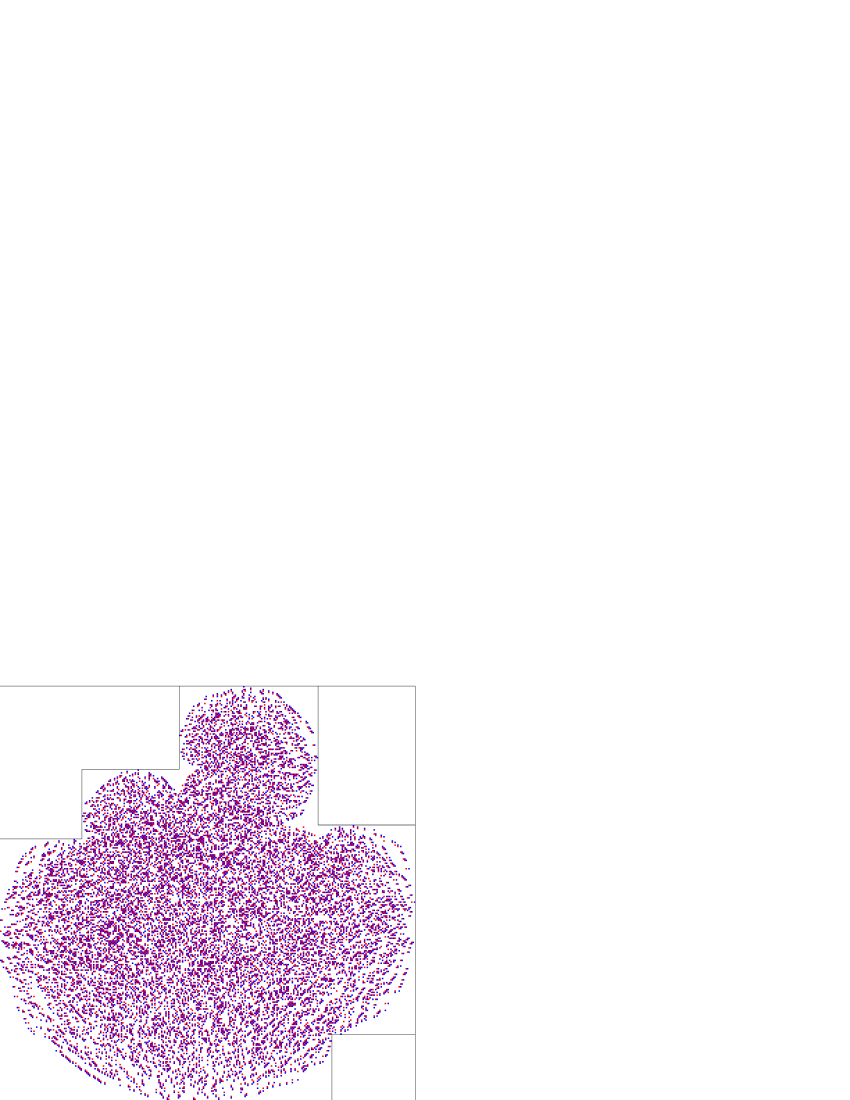
Figure 4. A typical configuration of the six-vertex model at ice point, $\mathsf{a}=\mathsf{b}=\mathsf{c}=1$, on a generic ‘digitally-convex’ portion of the square (here of size 300), with domain-wall boundary conditions. The side sizes, in counter-clockwise order, starting from the bottom-left corner, are 290, 60, 50, 70, 60, 100, 100, 70, 150, 60, 50, 240.

Numerical investigations show that, analogously to what happens in the same geometries for domino tilings, here we also have limit shapes and Arctic curves, with the feature, new w.r.t. the square domain, of having pairs of cusps in correspondence of concave angles (see Figure 4). Thus we have arcs of three types, connecting two cusps, a cusp and a contact point, or two contact points. We call an arc internal if it is of the first type, and external if it is of the second or third type.

Quite evidently, these domains can be seen as marginals of the $N\times N$ square domain, in which the frozen regions on the four corners have been constrained to contain the set-difference of the square and the new domain. The simplest realisation of this, consisting of a rectangular region cut off from the top-left corner, just coincides with the emptiness formation probability studied in [CP-07b] and subsequent papers, so that the study of this class of domains is promising.

The Tangent Method, in its abstraction outlined in Section 4.1, applies immediately to this setting, for what concerns external arcs. Let $\Lambda$ be such a domain, let us concentrate (say) on a given south side, and to the corner at its right endpoint. This may be a concave corner, and is thus followed by a west side, or a convex corner, followed by an east side. For definiteness, we put the origin of the coordinate axes at this corner. We aim to determine the (external) portion of the Arctic curve which is above this south side, and on the right of its contact point (if any), and so that the curve is ‘visible’ from the side, i.e. the tangent segment is contained within the domain. Call $H^{(r)}$, $h(z)$ and $r(z)$ the quantities associate to the one-point correlation function pertinent to this side, in analogy with the case of a square domain. Let the lattice coordinates be rescaled by the same choice of size parameter used for rescaling $r(z)$ from $h(z)$ (this may be, for example, the total number $N$ of horizontal lines). Then, on the same ground of rigour of the derivation for the square domain, and based on the suitable restating of the Assumption 3.1, we have

Conjecture 4.1.

For the system outlined above, the forementioned portion of the Arctic curve is the geometric caustic (envelope) of the one-parameter family of lines in the $(x,y)$-plane, in the parameter $z\in[1,+\infty)$,

$$F(x,y;z)=x-\frac{z(t^{2}-2\Delta t+1)}{(z-1)(t^{2}-2\Delta t+z)}y-r(z).$$ (4.7)

For arcs in other orientations, we have either the very same statement, or, if a reflection is involved, the analogous statement with $t\leftrightarrow t^{-1}$.

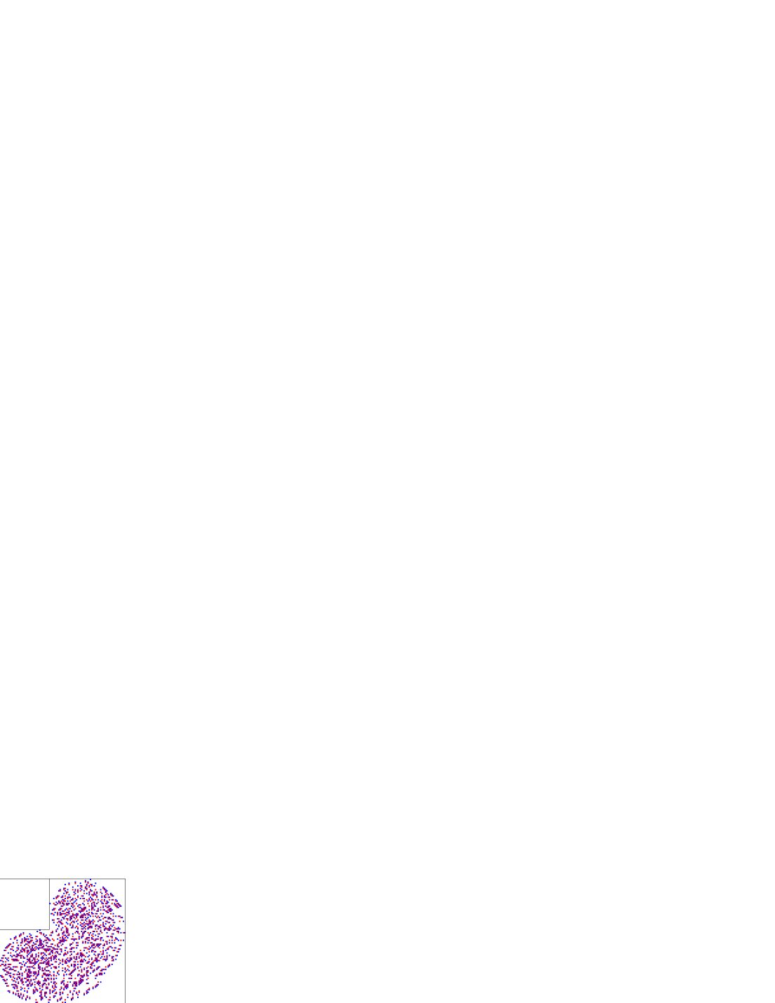
Figure 5. Left: a typical configuration on the square of size 100, with at square of size 40 removed from the top-left corner. Right: same, with the extra constraint that the south refinement position is $r=82$. This illustrates Conjecture 4.1, and its use in the Tangent Method.

5. The Arctic curve on the triangoloid domain

5.1. Why this model

At this point it shall be clear that the Tangent Method applies in a variety of circumstances. Essentially, all we need is that the model has a conservation law in the form of line conservation, that the behaviour of a single line is in the universality class of random directed walks, and, apparently, that the interaction among the lines is not of attractive type.

We have motivated already how the six-vertex model is a good prototype for this study: it is rich enough to go beyond the free-fermionic case, still it is probably the simplest exactly solvable model with these characteristics, with a continuous parameter (here $\Delta$) interpolating between universality classes.

We have also motivated the fact that, for obtaining a sensible thermodynamic limit, the easiest recipe is to consider a finite number of bundles of spectra lines, that intersect each other producing rectangular patches of the square grid, which are then arranged together.

Then, at the light of the discussion of the previous section, one should think that the simplest case next to treat would be the case of Figure 5. Too bad that, at the moment, we are not able to give the analytic expression of the Arctic curve for that domain. Indeed, even assuming Conjecture 4.1 to hold, the quantity $r(z)$ is not known for none of the three types of sides (up to symmetry) in this domain. What one would need in order to do so is a fine control on some generalised version of the emptiness formation probability (see [CPS-16]).

There is a lucky situation, that we call triangoloid domain, in which, although the domain seems somewhat more complicated than these other cases, at the ice point ($\mathsf{a}=\mathsf{b}=\mathsf{c}=1$) we have access to the refined enumeration. This occurs as a corollary of the dihedral Razumov–Stroganov correspondence [CS-11], present in that special domain, which allows to deduce the refined enumeration for all configurations altogether, from the known refined enumeration on the square domain, and the one for a specially simple subclass of configurations [CS-14].

The determination of the Arctic curve in this domain is thus possible, and is the subject of this section.

5.2. The model

Let $a$, $b$ and $c$ be three integers (not to be confused with the Boltzmann weights $\mathsf{a}$, $\mathsf{b}$, and $\mathsf{c}$ of the six-vertex model). Take three bundles of $a+b$, $b+c$, and $c+a$ lines, crossing each other, and use the resulting graph as a domain for the six-vertex model, that we call triangoloid, or three-bundle domain (see Fig. 6).

Figure 6. The $(a,b,c)$-triangoloid domain with domain wall boundary conditions, and a typical configuration. In this case $(a,b,c)=(2,3,4)$, and the south refinement position is $r=7$.

The internal faces of this graph are thus all squares, except for one triangle. We have a line of defects (denoted by a dashed line) going from this triagular face towards the north-west corner of the figure. Edges crossed by this line have arrows with opposite direction on the two sides. In other words, passing to the path representation, the two half-edges above and below the dashed line are either thick and thin, or thin and thick, respectively.

This is a special case of six-vertex model with edge defects, whose configurations are in fact covariant under a $\mathbb{Z}_{2}$ gauge in a way analogous to frustration in two-dimensional spin glasses (this is quickly reminded in Appendix E), and it is useful to keep in mind that only the endpoints of this line of defects have an intrinsic relevance.

We take domain-wall boundary conditions, that means here that arrows on consecutive external edges have equal orientation, unless we go through one corner, or we go through the defect line (this, consistently, makes a total of four changes of orientation, an even number as it should).

For this configuration of defects, the correspondence of Figure 1 between arrows and thick-line configurations is essentially preserved, and the thick paths are still directed, i.e., if oriented as outgoing from the west side and ingoing in the north side, may only perform north and east steps.

As defects act by inverting the thickness state of the adjacent edges, we must have an endpoint of a thick path at each and every defect. The boundary conditions force that, of the $a+b$ defects, exactly $a$ have the endpoint of a path that started from the west side (and, in fact, from the $a$ top-most edges of this side), and $b$ have the endpoint of a path that terminates at the north side (and, in fact, at the $b$ left-most edges of this side). The $c$ bottom-most edges of the west boundary and the $c$ right-most edges of the north boundary are connected by thick paths, that do not intersect, and pass all at the right of the triangular face.

Numerical simulations clearly show the emergence of an Arctic curve for triangoloids of large size. See Fig. 7 for an example. Not surprisingly, in a representation showing the collection of $\mathsf{c}$-vertices, there is no special feature occurring at the defect line, as, in light of Appendix E, this line is not intrinsic to the model (it can be moved around with a gauge transformation).

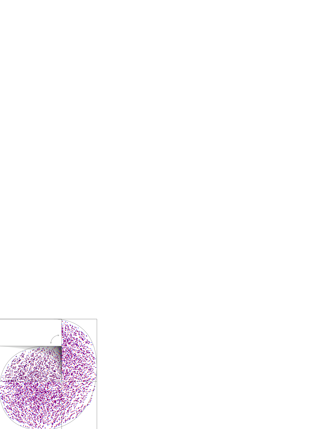
Figure 7. A typical configuration of the six-vertex model at ice-point, $\mathsf{a}=\mathsf{b}=\mathsf{c}=1$, on a $(a,b,c)$-triangoloid. The top-right $(a+b)\times(b+c)$ sub-domain is reproduced a second time, rotated by 90 degrees, under a gray shadow, to help visualising the continuity of the limit shape through the line of defects. Here $a=70$, $b=45$, $c=20$. In overlay, the analytic prediction of the Arctic curve.

There could be, in principle, something special happening in proximity of the triangular face, both because of the source of defects, and because of the curvature of the square lattice at this point. Apparently there are two regimes. When the three parameters $a$, $b$ and $c$ are comparable, nothing special seems to happen near to the triangle (in the case $a=b=c$ we just find back the three arcs of ellipse for the $\Delta=1/2$ and $t=1$ square of side $2a$, concatenated in the obvious way). When instead one parameter (say, $c$) is small with respect to the other two, a macroscopic frozen triangoloid region opens up around the triangular face (in the limit $c\ll a,b$ we recover again the Arctic curve for the square domain, this time at size $a+b$, plus a straight segment, of which we know the coordinates from the use of the Tangent Method in Section 3). This second limit, which is more subtle because it makes the Arctic curve only weakly-convex, is briefly discussed at the end of the section.

We can adapt the construction of Section 3 to the present case, by continuing the $a+2b+c$ vertical lines downward, adding below the triangoloid a bundle of $L-1$ horizontal lines, and modifying the boundary conditions as illustrated in Section 3 (or, alternatively, we could have used the local criterium established in Section 4.1).

As a result, the lower-right arc of the Arctic curve, delimited by the two contact points with the right and lower boundary, may be worked out along the lines of Conjecture 4.1, provided that we can evaluate the analogue of quantity $r(z)$ for the $(a,b,c)$-triangoloid.

5.3. The one-point boundary correlation function at ice point

From now on, we consider this model at ice-point, $\mathsf{a}=\mathsf{b}=\mathsf{c}=1$, that is $\Delta=1/2$, $t=1$.

As a consequence of the ice-rule, on the south and east sides, which are not disturbed by the defect line, there is yet again a unique refinement position. We will concentrate on the south one, that we denote with $r$, and that ranges over $1\leq r\leq a+2b+c$.

Let us denote the one-point boundary correlation function in this case as $H_{a,b,c}^{(r)}$. A result of [CS-14] is that, at the ice point,

$$H_{a,b,c}^{(r)}=\binom{3N-2}{N-1}^{-1}\binom{a+b+c-1}{b}^{-1}\\ \times\sum_{s=1}^{r}\binom{2N-s-1}{N-1}\binom{N+s-2}{N-1}\binom{c+r-s-1}{c-1}\binom{a+b-r+s-1}{a-1},$$ (5.1)

where $N:=a+b+c$, and $r\in\{1,\ldots,a+2b+c\}$. See Appendix D for details on the genesis and derivation of this expression.

We are interested in evaluating the asymptotic behaviour of (the logarithmic derivative of) the corresponding generating function,

$$h_{a,b,c}(z):=\sum_{r=1}^{a+2b+c}H_{a,b,c}^{(r)}z^{r-1}$$ (5.2)

in the limit of large triangoloid sizes, $a$, $b$, $c\to\infty$, with their ratios fixed. Let

$$a=\lceil N\alpha\rceil,\quad b=\lceil N\beta\rceil,\quad c=\lceil N\gamma\rceil,\quad r-s=\lfloor N\xi\rfloor,\quad s=\lceil N\eta\rceil,$$ (5.3)

with $\alpha,\beta,\gamma,\xi,\eta\in\mathbb{R}$, $\alpha,\beta,\gamma>0$, $\alpha+\beta+\gamma=1$, $0<\xi<1+\beta$, $0<\eta<1+\beta-\eta$.

The sums appearing in (5.1) and (5.2) can be interpreted as Riemann sums, that in the scaling limit turn into a two-dimensional integral. Simple Stirling approximation shows the log-concavity of the integrand, so that in the limit the integral is dominated by the contribution of a unique non-singular saddle point. We define the ‘action’:

$$S(\xi,\eta;\alpha,\beta,\gamma,z):=\\ \lim_{N\to\infty}\frac{1}{N}\ln\left[\frac{(2N-s-1)!(N+s-2)!(c+r-s-1)!(a+b-r+s-1)!}{(N-s)!(s-1)!(r-s)!(b-r+s)!}z^{r-1}\right],$$ (5.4)

where we have ignored factors that do not depend on $\xi$ or $\eta$.

From standard saddle-point arguments, it follows that

$$\begin{split}r_{\alpha,\beta,\gamma}(z)&:=\lim_{N\to\infty}\frac{1}{N}z\frac{\mathrm{d}}{\mathrm{d}z}\ln h_{a,b,c}(z)\\ &=\xi_{sp}+\eta_{sp},\end{split}$$ (5.5)

where $\xi_{sp}$, $\eta_{sp}$, are the solutions of the two saddle-point equations:

$$z =\frac{\xi(1-\gamma-\xi)}{(\beta-\xi)(\gamma+\xi)}, z =\frac{\eta(2-\eta)}{1-\eta^{2}},$$ (5.6)

namely,

$$\xi_{sp} =\frac{(\gamma-\beta)z+\alpha+\beta-\sqrt{[(\gamma-\beta)z+\alpha+\beta]^{2}-4\gamma\beta z(1-z)}}{2(1-z)}$$ (5.7a)

$$\eta_{sp} =\frac{1-\sqrt{z^{2}-z+1}}{1-z}$$ (5.7b)

The signs of the square roots are fixed by the condition that for large real $z$ the quantity $r_{\alpha,\beta,\gamma}(z)$ should tend to the value:

$$\lim_{z\to+\infty}(\xi_{sp}+\eta_{sp})=\frac{\alpha+2\beta+\gamma}{\alpha+\beta+\gamma}=1+\beta.$$ (5.8)

This condition follows directly from definitions (5.2) and (5.5), assuming that the limits $N\to\infty$ and $z\to\infty$ may be interchanged.

5.4. The Arctic curve for the six-vertex model on the triangoloid

We are now ready to use Conjecture 4.1. Setting $\Delta=1/2$, $t=1$ in (3.2), and inserting the quantity $r_{\alpha,\beta,\gamma}(z)$, see (5.5), expressed as the sum of the solutions (5.7), we obtain the family of lines

$$y=(z-1)x+1-\sqrt{z^{2}-z+1}+\frac{1}{2}\left[(\gamma-\beta)z+\alpha+\beta\right]\\ -\frac{1}{2}\sqrt{[(\gamma-\beta)z+\alpha+\beta]^{2}+4\gamma\beta z(z-1)},\qquad z\in[1,\infty).$$ (5.9)

The corresponding geometric caustic has the parametric form

$$\left\{\begin{array}[]{l}x=1+\beta-\zeta(z;\alpha,\beta,\gamma)\\ \\ y=\zeta(\frac{z}{z-1};\beta,\alpha,\gamma)\end{array}\right.\qquad z\in[1,\infty)$$ (5.10)

where

$$\zeta(z;\alpha,\beta,\gamma)=\frac{3-\alpha}{2}-\frac{2z-1}{2\sqrt{z^{2}-z+1}}-\frac{(1-\alpha)^{2}z+\alpha\gamma-\beta}{2\sqrt{[(\gamma-\beta)z+\alpha+\beta]^{2}-4\gamma\beta z(1-z)}}$$ (5.11)

This describes the south-east arc of the Arctic curve of the six-vertex model at ice-point, on the triangoloid, between the two contact points on the east and south boundaries. As evinced from the $z=1$ limit of the expression above, and more easily from (5.1), the south contact point is at the rescaled coordinate $(\kappa,0)$, with $\kappa=\frac{\alpha+\beta+\gamma}{2}+\frac{\beta\gamma}{\alpha+\gamma}$.

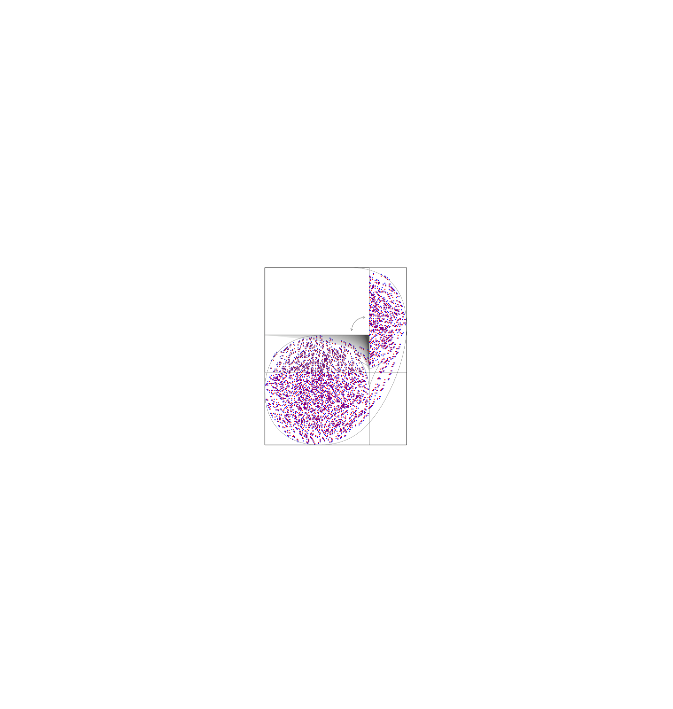
Figure 8. Analogue of Figure 7 for a different aspect ratio. In this case $a=79$, $b=39$, $c=3$. In overlay, the analytic prediction of the external portion of the Arctic curve, and the curve obtained by the ‘wild guess’ described in the text, which reproduces the internal portion of the Arctic curve in the limit $\gamma\to 0$.

The other two arcs of the curve can be obtained straighforwardly by cyclic permutation of the parameters $\alpha$, $\beta$, $\gamma$ in (5.10), (5.11), and appropriate relabeling of coordinate axis. The result is plotted against a numerical simulation in Fig. 7.

We have already mentioned that, in the limit $c\ll a,b$, we shall obtain back the Arctic curve of the square, reproduced within the south-west and north-east rectangular sub-domains w.r.t. Figure 6 (cut towards the line of defects), plus a straight segment, on the south-east side, tangent to both copies of the Arctic curve (the numerical simulation of Figure 8 is not far from this limit). This may seem mysterious at first, as, for positive values of the size parameters, the resulting curve is convex.

In order to see how this limit develops a singularity, consider the expression (5.11) for $\gamma\to 0^{+}$ (and thus $\alpha+\beta\to 1^{-}$). In this limit we have

$$\zeta(z;1-\beta,\beta,0)=1+\frac{\beta}{2}-\frac{2z-1}{2\sqrt{z^{2}-z+1}}+\frac{\beta}{2}\frac{1-\beta z}{\sqrt{(1-\beta z)^{2}}}$$ (5.12)

and the quantity $\frac{1-\beta z}{\sqrt{(1-\beta z)^{2}}}$ has to be interpreted as the sign of $1-\beta z$. Thus the $x(z)$ coordinate function has a jump for $z=1/\beta$, and, consistently, $y(z)$ has a jump for $z/(z-1)=1/\alpha=1/(1-\beta)$, i.e. again for $z=1/\beta$.

In fact, in the limit $\gamma\to 0$, if in both entries of the parametric solution (5.10) we use a function $\zeta$ with the other sign of square root in the last summand, w.r.t. the definition in (5.11), we obtain a curve that approaches the known internal part of the Arctic curve (see Figure 8). However, this wild guess, besides being not theoretically motivated, must also be wrong in some respect when $\gamma$ is small but positive. In this case the curve has the appropriate qualitative behaviour (including the cusps, and some of the consistency checks), but the two endpoints of the curve, when folded around the conical singularity, miss each other by a distance $\mathcal{O}(\gamma)$, namely $\gamma\frac{1-\alpha\beta}{(\alpha+\gamma)(\beta+\gamma)}$.

6. Conclusions

Which models next?

This paper sets the basis for a method aimed at the determination of the Arctic curve in statistical mechanics models on planar graphs, with (piecewise) local translational invariance of the lattice and weights, showing phase separation phenomena, in light of a conserved quantity in the associated transfer matrix, that can be seen as the number of lines in a suitable line representation. This is the case for a variety of dimer or free-fermionic models (for which, however, in most cases more powerful general methods already exist), for the six-vertex model, treated here in detail, and for variants of it in which some spectral lines may contain higher spin or $q$-bosons.

The constraint of having a line representation may appear as a strong limitation of the method. Let us however stress how, up to bijections, families of non-intersecting (possibly interacting) lattice paths constitute a very general and flexible language for representing a variety of mathematical structures, ranging from Young diagrams [RS-16] and tableaux [PR-07] to $Q$-systems and cluster algebras [DFK-10].

The application of the Tangent Method to quite different classes of models, and the study of its interplay with other existing techniques, is in our opinion a direction of research deserving to be explored.

What more for the six-vertex model?

It shall be clear that also for the six-vertex model, the main subject of this paper, the analysis is far from complete. A variety of domains still asks for the determination of their Arctic curve, and in particular it would be quite interesting to obtain the analytic expression for an Arctic curve in a domain presenting cusps, for a system out of free-fermionic points. As we said, the main obstacle in these derivations is the lack of knowledge of refined enumerations, called here one-point boundary correlation functions. The most promising candidate seems to be the six-vertex model in the domain presented in Figure 5. We hope that some progress in this direction will be available in the light of our results on a generalisation of the Emptiness Formation Probability observable [CPS-16].

We also remind that the Tangent Method, in its present formulation is not adapted to the determination of the internal portions of the Arctic curve, i.e. the arcs between two cusps. Or the internal components of Arctic curves in the cases where, as for the triangoloid domain, there are internal frozen regions. We hope that the puzzling features of the internal component of the curve outlined at the end of Section 5 may be clarified in the future.

Which Tangent Method?

Another natural question is how to make precise the assumptions listed in Section 3.2. In principle, the short discussion following the assumption gives a clear roadmap to this task. However, a further aspect of the method that we have not discussed here is the fact that it exists in several variants, which exploit in slightly different ways the peculiar behaviour of one thick path that, in one way or another, has been singled out from the liquid region by mean of a marginalisation on a boundary observable.

The version described in this paper, that could be called Geometric Tangent Method, is the one which is visually more clear (especially in its realisation with an auxiliary external domain, as in Section 3). However, we have devised also an Entropic Tangent Method, that establishes a criterium based on the locality of the free energy, and performs some ‘surgery’ of domains for comparing the free energy of different refined ensembles. We have an Algorithmic Tangent Method, adapted to those cases in which the configurations are obtained from iterated applications of substitutional rules. Finally, we have a promising Doubly-refined Tangent Method, which exploits (when available) the two-point boundary correlation function, the two points being on two consecutive sides of the boundary, this providing a geometric setting in which the complicancy of the contact between the tangent path and the liquid region is eliminated.

All these different methods come with slightly different technical requirements, for satifying the associated variants of the Tangent Assumption, and the comparison between the different methods is still to be completely investigated, in a trade off between the mathematical control on the assumptions, and the domain of applications.

Appendix A Weighted enumeration of directed lattice paths

We recall here some classical results in analytic combinatorics, concerning the enumeration of two-dimensional directed lattice paths in the square lattice, weighted according to the number of ‘corners’, and recast them in a form suitable for our purposes.

A directed lattice path $\gamma:(0,0)\to(x,y)$ is a path on the square lattice, starting in $(0,0)$ and arriving in $(x,y)$, and whose only allowed steps are $(1,0)$, or ‘east’, and $(0,1)$, or ‘north’. If the path visits the vertices $\{v_{i}\}_{0\leq i\leq x+y}$, we thus have $v_{i+1}-v_{i}\in\{(1,0),(0,1)\}$, $v_{0}=(0,0)$ and $v_{x+y}=(x,y)$.

For $x$ and $y$ nonnegative integers, the number of such paths reaching the point of coordinates $(x,y)$ is clearly

$$P(x,y)=\binom{x+y}{y}.$$ (A.1)

We now assign to each path $\gamma$ a weight $\omega^{c(\gamma)}$, where $c(\gamma)$ is the number of ‘north-east corners’, i.e., of vertices $v_{i}$, $0<i<x+y$ preceeded and followed by a north- and an east-step, respectively, $v_{i}=v_{i-1}+(0,1)=v_{i+1}-(1,0)$. We want to evaluate the weighted enumeration

$$P_{\omega}(x,y):=\sum_{\gamma}\omega^{c(\gamma)}.$$ (A.2)

Let $\mathcal{N}(x,y,l)$ denote the number of directed lattice paths reaching $(x,y)$, with exactly $l$ north-east corners. It is clear that these paths are in bijection with pairs of subsets of $I\subseteq\{0,\ldots,x-1\}$ and $J\subseteq\{1,\ldots,y\}$, both of cardinality $l$ (the $k$th corner is at $v=(i_{k},j_{k})$, where $i_{k}$ and $j_{k}$ are the $k$th element of sets $I$ and $J$, in order). This leads immediately to

$$\mathcal{N}(x,y,l)=\binom{x}{l}\binom{y}{l},$$ (A.3)

and, hence,

$$P_{\omega}(x,y)=\sum_{l\geq 0}\binom{x}{l}\binom{y}{l}\omega^{l}.$$ (A.4)

Obviously, in the above sum all terms with $l>\mathrm{min}\{x,y\}$ vanish. Note also that the formula above consistenlty reduces to (A.1) at $\omega=1$, as a result of Chu-Vandermonde formula.

For our purposes, it is now convenient to slightly modify our definition by adding to each lattice path $\gamma$ an east step just before the origin, and a north step next to the final point $(x,y)$. We denote this modified path by $\tilde{\gamma}$. Manifestly, the new path does not have any extra north-east corner.

We now want to count paths $\tilde{\gamma}$, according to two statistics: number $s(\tilde{\gamma})$ of ‘straights’, i.e., of vertices $v_{i}$, $0\leq i\leq x+y$, such that the preceeding and following steps are both north or both east, and the number $t(\tilde{\gamma})$ of ‘turns’, i.e., of vertices $v_{i}$, $0\leq i\leq x+y$, such that the preceeding and following steps are either north and east, or east and north. It is clear that

$$s(\tilde{\gamma})+t(\tilde{\gamma})=x+y+1,$$ (A.5)

$$t(\tilde{\gamma})=2c(\tilde{\gamma})+1.$$ (A.6)

which makes manifest the homogeneity of this double-statistics, and its connection with the previous formula (A.4)

Let us now assign weights $\mathsf{b}/\mathsf{a}$ and $\mathsf{c}/\mathsf{a}$ to each straight and turn, respectively. For what we said, the corresponding weighted enumeration of paths

$$P_{\mathsf{a},\mathsf{b},\mathsf{c}}(x,y):=\sum_{\tilde{\gamma}}\Big{(}\frac{\mathsf{b}}{\mathsf{a}}\Big{)}^{s(\tilde{\gamma})}\Big{(}\frac{\mathsf{c}}{\mathsf{a}}\Big{)}^{t(\tilde{\gamma})}.$$ (A.7)

is just given by

$$P_{\mathsf{a},\mathsf{b},\mathsf{c}}(x,y) =\sum_{l\geq 0}\mathcal{N}(x,y,l)\Big{(}\frac{\mathsf{b}}{\mathsf{a}}\Big{)}^{x+y-2l}\Big{(}\frac{\mathsf{c}}{\mathsf{a}}\Big{)}^{2l+1}$$ (A.8)

$$=\Big{(}\frac{\mathsf{b}}{\mathsf{a}}\Big{)}^{x+y+1}\sum_{l\geq 0}\binom{x}{l}\binom{y}{l}\Big{(}\frac{\mathsf{c}}{\mathsf{b}}\Big{)}^{2l+1}.$$ (A.9)

Again, in the above sum all terms with $l>\mathrm{min}\{x,y\}$ vanish. This formula can be applied directly in the context of the six-vertex model, with Boltzmann weights $\mathsf{a}$, $\mathsf{b}$, $\mathsf{c}$ as in Section 2.2. Use of (2.3) to express the Boltzmann weights in terms of the parameters $\Delta$ and $t$ leads to equation (3.5).

Appendix B Alternating Sign Matrices

An Alternating Sign Matrix (ASM) of size $n$ is an $n\times n$ matrix valued in $\{0,\pm 1\}$, such that: (i) non-zero entries alternate in sign along rows and columns; (ii) the sum of entries along each row or column is $+1$ [pzjhdr].

Let $A_{n}$ be the number of ASMs of size $n$. It is well known that [Ze-96, Ku-96]:

$$A_{n}=\prod_{j=0}^{n-1}\frac{(3j+1)!}{(n+j)!}.$$ (B.1)

ASM of sixe $n$ are in bijection with the configurations of the six-vertex model on the $n\times n$ lattice, with domain wall boundary conditions (entries $+1$ and $-1$ in the ASM corresponding to $w_{6}$ and $w_{5}$ vertices in the six-vertex model, respectively). Thus the partition function of the model [I-87], when evaluated at the ice point, $\mathsf{a}=\mathsf{b}=\mathsf{c}=1$, coincides with $A_{n}$.

The one-point correlation function $H_{N}^{(r)}$, then, is related to the so-called refined enumerations: Let $A_{n}(r)$ be the number of ASM of size $n$ such that the sole non-zero entry in the bottom row is in the $r$th column, then it is well-known that [Ze-96b]:

$$A_{n}(r)=A_{n}\binom{2n-r-1}{n-1}\binom{n+r-2}{n-1}\binom{3n-2}{n-1}^{-1}.$$ (B.2)

and it is clear that $H_{n}^{(r)}|_{\Delta=\frac{1}{2},t=1}=A_{n}(r)/A_{n}$.

Then, in the formalism of Section 3.4, the partition functions $Z^{(+)}_{N,k}$ and $Z^{(-)}_{N,L,k}$ just reduce to $A_{N}(k)$, as in (B.2) above, and to the binomial coefficient $P(r,L)$, as in (A.1). In particular, one can calculate

$$r_{\rm ASM}(z):=\lim_{N\to\infty}\frac{1}{N}z\frac{\mathrm{d}}{\mathrm{d}z}\ln\left(\frac{1}{A_{N}}\sum_{r=1}^{N}A_{N}(r)z^{r-1}\right)=\frac{\sqrt{z^{2}-z+1}-1}{z-1},$$ (B.3)

which gives the family of lines

$$F_{\rm ASM}(x,y;z)=x-\frac{1}{z-1}y-r_{\rm ASM}(z),\qquad z\in[1,+\infty).$$ (B.4)

The corresponding geometric caustic reproduces (the lower-right quarter of) the limit shape of ASMs, first derived in [CP-08].

Appendix C The Arctic curve for lozenge tilings of a hexagon

As a simple application of the Tangent Method, in a framework different from the six-vertex model, we derive here the Arctic curve for lozenge tilings of a hexagon, or equivalently, the frozen boundary of the limit shape of boxed plane partitions, which is an ellipse, thus recovering a result of Cohn, Larsen and Propp [CLP-98].

Let us call a $(a,b,c)$-hexagon the hexagonal portion of the triangular lattice whose side lengths are $a,b,c,a,b,c$ in clockwise order, and let us adopt the convention that the horizontal sides are those of length $b$.

We are interested in the tilings of this hexagon with rhombi of side length 1, i.e. obtained from the union of two neighbouring triangles of the lattice, called lozenges. Referring to the orientation of the longest diagonal, we have one type of vertical lozenges, and two orientations for oblique lozenges. In this Appendix we shall adapt to the notations of [CLP-98].

Let $M_{a,b,c}$ be the number of lozenge tilings of a $(a,b,c)$-hexagon. We recall that

$$M_{a,b,c}=\prod_{j=0}^{a-1}\prod_{k=0}^{b-1}\prod_{l=0}^{c-1}\frac{j+k+l+2}{j+k+l+1}=\prod_{j=0}^{b-1}\frac{j!(j+a+c)!}{(j+a)!(j+c)!},$$ (C.1)

a classical result of MacMahon.

In order to apply the Tangent Method, we need some particular refinement of MacMahon formula. These very same quantities have already been evaluated in [EKLP-92, CLP-98], exploiting a nice description of the lozenge tilings in terms of semi-strict Gelfand–Tsetlin patterns [GT-50], which we now recall.

Define the $(n,k)$-trapezoid as the isosceles trapezoid region of the triangular lattice, with sides $k,n,n+k,n$, in order. We will represent this with the short basis on the bottom, and the long basis on top. Tilings of this region with lozenges and unit triangles that maximise the number of lozenges have exactly $n$ triangles. We will consider such tilings, under the restriction that all these triangles are adjacent to the long basis. For a given tiling, we denote by $\mathbf{x}=(x_{1},\dots,x_{n})$, with $1\leq x_{1}<x_{2}<\dots<x_{n-1}<x_{n}\leq n+k$, the horizontal coordinates of these triangles. See Fig. 9 for an example. Each tiling of the above defined trapezoid can be equivalently viewed as a semi-strict Gelfand–Tsetlin pattern with top row $\mathbf{x}$, see, e.g., [CLP-98].

Figure 9. A lozenge tiling of a $(n,k)$-trapezoid as described in the text, with $(n,k)=(4,6)$ and ${\bm{x}}=(1,3,7,8)$.

Let $V_{n}(\mathbf{x})$ be the number of tilings of the $(n,k)$-trapezoid with triangular tiles located at $\mathbf{x}$. A well-known formula, due to Gelfand and Tsetlin, states [GT-50, EKLP-92, CLP-98]:

$$V_{n}(\mathbf{x})=\prod_{1\leq i<j\leq n}\frac{x_{j}-x_{i}}{j-i}.$$ (C.2)

The number of tilings does not depend on $k$, as long as $k>x_{n}-n$, since for non-minimal values of $k$ there is a frozen region on the right side. Similarly, it is invariant under an overall translation $x_{j}\to x_{j}+l$ because of a frozen region on the left side.

It is easy to see that, under the choice $k=b$, $n=a+c$, $\mathbf{x}=(1,\dots,a,a+b+1,\dots,a+b+c)$, two frozen equilateral triangles, of side $a$ and $c$, appear in the two upper corners of the trapezoid, and what is left to tile (with lozenges only) is exactly a $(a,b,c)$-hexagon. Indeed, in this case, the Gelfand–Tsetlin formula (C.2) reduces, after some manipulations, to MacMahon formula, equation (C.1). We shall now consider two other specializations of the Gelfand–Tsetlin formula, that lead to refined enumerations of lozenge tilings of a hexagon (i.e., in the language of this paper, to one-point boundary correlation function), and are thus adapted to the application of the Tangent Method.

The first case corresponds to the particular choice $\mathbf{x}=(1,\dots,\hat{r},\dots$, $a+1,a+b+1,\dots,a+b+c)$. With respect to the MacMahon realisation, one triangle has been moved from $r$ to $a+1$. We shall denote the number of tilings of this region as $M_{a,b,c}(r)$, which is just the shortcut

$$M_{a,b,c}(r)=V_{a+c}(1,\dots,\hat{r},\dots,a+1,a+b+1,\dots,a+b+c).$$ (C.3)

Clearly we have the extremal values

$$M_{a,b,c}(a+1) =M_{a,b,c}, M_{a,b,c}(1) =M_{a,b-1,c}.$$ (C.4)

In working out explicit expressions, it is significantly simpler to evaluate ratios. In the present case, an elementary calculation gives:

$$\frac{M_{a,b,c}(r)}{M_{a,b,c}}\equiv\frac{M_{a,b,c}(r)}{M_{a,b,c}(a+1)}=\binom{a}{r-1}\binom{b+c-1}{c}\binom{a+b+c-r}{c}^{-1},$$ (C.5)

with $r\in\{1,\dots,a+1\}$.

The second case of interest is the enumeration of the lozenge tilings of the $(a,b,c)$-hexagon, refined according to the location of the unique vertical lozenge occuring in the vicinity of the top boundary. Cutting away the top-most row of the lattice, this can be rephrased as the enumeration of lozenge tilings of a trapezoid with bases $b$ and $a+b+c-1$, heigth $a+c-1$, and triangular tiles located at $\mathbf{x}=(1,\dots,a-1,a+r,a+b+1,\dots,a+b+c-1)$. Let us denote this number as $N_{a,b,c}(r)$, where $r\in\{0,1,\dots,b\}$, which is just the shortcut

$$N_{a,b,c}(r)=V_{a+c-1}(1,\dots,a-1,a+r,a+b+1,\dots,a+b+c-1),$$ (C.6)

and has the extremal cases

$$N_{a,b,c}(0) =M_{a,b,c-1}, N_{a,b,c}(b) =M_{a-1,b,c}.$$ (C.7)

Yet again, considering ratios we get

$$\frac{N_{a,b,c}(r)}{N_{a,b,c}(0)}=\binom{a+r-1}{a-1}\binom{b+c-r-1}{c-1}\binom{b+c-1}{c-1}^{-1},$$ (C.8)

which in turn leads to

$$\frac{N_{a,b,c}(r)}{M_{a,b,c}}=\binom{a+r-1}{a-1}\binom{b+c-r-1}{c-1}\binom{a+b+c-1}{b}^{-1},$$ (C.9)

with $r\in\{0,\dots,b\}$

The Tangent Method is better visualised through the construction of directed non-intersecting lattice paths, which in this case arise through a well-known bijection. For each oblique lozenge, let us draw a segment connecting the midpoints of its horizontal sides. Clearly, these segments concatenate to form continuous paths on the triangular lattice (with steps using only two directions of the lattice, i.e. in fact being directed paths). In the case of the $(n,k)$-trapezoid with vector $\mathbf{x}$, each lozenge tiling can be now viewed as a configuration of $k$ non-intersecting paths, connecting the $k$ points located at $1,\dots,k$ on the short basis with those $k$ points on the long basis which are at the complement set w.r.t. $\mathbf{x}$.

In particular, the choice $\mathbf{x}=(1,\dots,a,a+b+1,\dots,a+b+c)$ gives a lattice path description of the lozenge tilings of the $(a,b,c)$-hexagon, with $b$ paths connecting the two horizontal sides, on sequences of consecutive points. The choice $\mathbf{x}=(1,\dots,\hat{r},\dots,a+1,a+b+1,\dots,a+b+c)$, corresponding to our first refinement, $M_{a,b,c}(r)$, see (C.5), has $b$ paths, starting all contiguous on the short basis, and arriving all contiguous on the long basis, with the exception of the left-most path, that arrives at $r$, as illustrated in Figure 10.

This special path is directed. Thus, in particular, it crosses exactly once the lattice line that goes in north-east direction, starting from position $c-1$ on the west side of the trapezoid, this occurring with an oblique lozenge sheared towards the left, see Fig. 10. Let us call cut-line this special line on the lattice, and call $s$ the distance of this special lozenge from the left side of the triangoloid.

Figure 10. A lozenge tiling of the $(n,k)$-trapezoid, with $(n,k)=(9,6)$. The locations of the triangular tiles $\mathbf{x}$ has been chosen to provide the refined enumeration $M_{a,b,c}(r)$, with $(a,b,c)=(4,5,4)$, and $r=3$. In the non-intersecting lattice path description of lozenge tilings, the left-most path, in a thicker green line in the picture, connects the left-most horizontal edge on the bottom (short) basis with position $r$ on the top (long) basis. Inside the $(a,b,c)$-hexagon, there is a unique oblique lozenge that crosses the dotted line of length $a+1$. We denote its distance from the bottom-left side of the trapezoid by $s$ (thus $s\in\{0,\dots,a-1\}$). Here $s=1$.

Within the ideas of the Tangent Assumption 3.1, in the large volume limit this path leaves the Arctic curve tangentially, and reaches the (given) position $r$ while crossing at a (random) value $s$, that concentrates on some value $s_{\rm sp}(r)$, up to sub-linear fluctuations (in fact, of order $N^{\frac{1}{2}}$). As $r$ varies, the function $s_{\rm sp}(r)$ allows to identify a family of straight lines, all tangent to the Arctic curve, which thus determine it through the construction of their caustic.

Any configuration can be decomposed into a part above the cut-line, and a part below. Say we have $Z_{1}(s)$ configurations in the part below, and $Z_{2}(r,s)$ configurations in the part above. We can recognise $Z_{1}(s)$ as the refined enumeration $N_{a,b,c}(s)$, under the substitution $(a,b,c)\to(c,a,b)$, and, quite trivially, $Z_{2}(r,s)$ just as binomial coefficient:

$$Z_{1}(s) =N_{c,a,b}(s), Z_{2}(r,s) =\binom{a-s}{a-r+1}.$$ (C.10)

On the other side, the refined enumeration $M_{a,b,c}(r)$, already evaluated in (C.5), is just

$$M_{a,b,c}(r)=\sum_{s}Z_{1}(s)Z_{2}(r,s)$$ (C.11)

which leads to the (not completely trivial) identity

$$\sum_{s=0}^{r-1}\binom{a-s}{a-r+1}\binom{c+s-1}{c-1}\binom{a+b-s-1}{b-1}=\\ \binom{a}{r-1}\binom{b+c-1}{c}\binom{a+b+c-1}{a}\binom{a+b+c-r}{c}^{-1},$$ (C.12)

holding for any $a$, $b$, $c$ integers, and $r\in\{1,\dots,a+1\}$.

Let us investigate the implications of identity (C.12) in the ‘thermodynamic limit’, i.e. when the hexagon has large size, and the ratios of the sides is kept fixed. Let

$$a =\lceil N\alpha\rceil, b =\lceil N\beta\rceil, c =\lceil N\gamma\rceil, r =\lceil N\xi\rceil, s =\lfloor N\eta\rfloor,$$ (C.13)

with $\alpha,\beta,\gamma,\xi,\eta\in\mathbb{R}$, $\alpha,\beta,\gamma>0$, and $0<\eta<\xi\leq\alpha$. When the overall scale factor $N$ is large, binomials can be replaced with the dominant term in Stirling formula, while the left-hand side, interpreted as Riemann sum, can be rewritten as an integral and evaluated in the saddle-point approximation. The saddle-point equation is simply

$$\frac{(\gamma+\eta)(\xi-\eta)}{\eta(\alpha+\beta-\eta)}=1$$ (C.14)

with solution

$$\eta_{sp}=\frac{\gamma\,\xi}{\alpha+\beta+\gamma-\xi},\qquad\xi\in[0,\alpha].$$ (C.15)

As $\xi$ varies over $[0,\alpha]$, $\eta_{sp}$ ranges over $[0,\alpha\gamma/(\beta+\gamma)]$, monotonically. Recalling that $\xi$ and $\eta$ actually parameterize the location of two points in the ‘rescaled’ plane, the saddle-point solution defines a family of pairs of points, or equivalently, a family of lines, parameterized by $\xi\in[0,\alpha]$. According to the Tangent Assumption, the corresponding geometric caustic is exactly the Arctic curve we are looking for (more precisely, its west arc, between the two contact points with the sides of the hexagon of length $a$ and $c$).

Adapting to the notations of [CLP-98], we introduce a Cartesian coordinate system, with origin at the center of the rescaled, $(\alpha,\beta,\gamma)$-hexagon. One can check that the sides of the hexagon lie on the lines $y=\frac{\sqrt{3}}{2}(2x+\beta+\gamma)$, $y=\frac{\sqrt{3}}{4}(\alpha+\gamma)$, $y=\frac{\sqrt{3}}{2}(-2x+\alpha+\beta)$, $y=\frac{\sqrt{3}}{2}(2x-\beta-\gamma)$, $y=\frac{\sqrt{3}}{4}(-\alpha-\gamma)$, $y=\frac{\sqrt{3}}{2}(-2x-\alpha-\beta)$. In such coordinate system the two points parameterized by $\xi$ and $\eta$ have coordinates

$$\left(\frac{4\xi-3\alpha-2\beta-\gamma}{4},\frac{\sqrt{3}}{2}\frac{\alpha+\gamma}{2}\right),\qquad\left(\frac{2\eta-\alpha-2\beta-\gamma}{4},\frac{\sqrt{3}}{2}\frac{2\eta+\gamma-\alpha}{2},\right),$$ (C.16)

respectively. Correspondingly, the family of lines selected by the saddle-point solution (C.15) has equation

$$2\left[(\alpha(\alpha+\beta+\gamma)-(\alpha+\gamma)\xi\right]x+\frac{2}{\sqrt{3}}\left[\alpha(\alpha+\beta+\gamma)-(3\alpha+2\beta+\gamma)\xi+2\xi^{2}\right]y\\ +\left[\alpha(\alpha+\beta)(\alpha+\beta+\gamma)-2\alpha(\alpha+\beta+\gamma)\xi+(\alpha+\gamma)\xi^{2}\right]=0$$ (C.17)

with parameter $\xi\in[0,\alpha]$. It is easy to verify that at $\xi=0$ and $\xi=\alpha$, we recover the lines on which lie the left sides of the hexagon of rescaled length $\gamma$ and $\alpha$, respectively.

A tedious but elementary calculation immediately leads to the parametric form of the corresponding geometric caustic,

$$x =\frac{1}{4}\,\frac{2\beta\gamma+(\alpha+2\beta-\gamma)(\alpha+\beta-2\xi)+\left(1-\frac{\gamma}{\alpha}\right)\left(1+\frac{\beta}{\alpha+\beta+\gamma}\right)\xi^{2}}{(\alpha+\beta-2\xi)+\alpha^{-1}\left(1-\frac{\beta}{\alpha+\beta+\gamma}\right)\xi^{2}},$$ (C.18)

$$y =\frac{\sqrt{3}}{4}\,\frac{2\alpha\beta+(\alpha+\gamma)(\alpha-\beta-2\xi)+\left(1+\frac{\gamma}{\alpha}\right)\left(1-\frac{\beta}{\alpha+\beta+\gamma}\right)\xi^{2}}{(\alpha+\beta-2\xi)+\alpha^{-1}\left(1-\frac{\beta}{\alpha+\beta+\gamma}\right)\xi^{2}},$$ (C.19)

where again $\xi\in[0,\alpha]$. This indeed describes a portion of the ellipse inscribed in the rescaled hexagon, namely that arc delimited by the contact points of the ellipse with the two forementioned sides of the hexagon. Eliminating the parameter $\xi$, we obtain the equation $E_{\alpha,\beta,\gamma}(x,y)=0$, where $E_{\alpha,\beta,\gamma}(x,y)$ is the polynomial

$$3\alpha\beta\gamma(\alpha+\beta+\gamma)-3(\alpha+\gamma)^{2}x^{2}+2\sqrt{3}(\alpha+\beta+\gamma)(\alpha-\gamma)xy-[(\alpha+2\beta+\gamma)^{2}-4\alpha\gamma]y^{2}$$ (C.20)

introduced in [CLP-98], and whose zero-set is indeed the ellipse inscribed in the $(\alpha,\beta,\gamma)$-hexagon.

Observe that, although in principle the Tangent Method shall have derived only one portion of the Arctic curve, the polynomial equation above describes the full Arctic ellipse of the model. As mentioned above, the possibility of extending one arc to the full curve just by analytic continuation is a special feature of free-fermionic systems [KO-05], which, as seen also from our explicit results on the six-vertex model, unfortunately seems to fail for other universality classes.

Let us stress the fact that in [CLP-98] the authors perform the analysis of the asymptotic behaviour of a much more complex refined enumeration of the lozenge tilings. On one side, that derivation is much more complicated than ours. But, most relevant, on the other side it allows to derive the whole limit shape of the model, where our restriction of the analysis to a suitably-chosen boundary refinement, with just one parameter, allows to obtain just the Arctic curve, i.e. the frozen boundary of the limit shape. It was not clear a priori, from [CLP-98], that a shorter track existed to extract the Arctic curve without solving the full limit-shape problem.

Appendix D Some results for the six-vertex model on a triangoloid

The six-vertex model at ice-point, $\mathsf{a}=\mathsf{b}=\mathsf{c}=1$, on the $n\times n$ square lattice with domain wall boundary conditions can be reformulated, through a simple bijection, in terms of fully-packed loops (FPL) on the same underlying graph, with alternating boundary conditions. This relation plays a crucial role in the formulation [RS-04] and proof [CS-11] of (the dihedral case of) the Razumov–Stroganov correspondence, which concerns the enumeration of these configurations according to their link pattern.

A major ingredient in the proof is the notion of gyration, an operation that can be performed on FPL configurations, and was used in [Wi-00] to prove the dihedral symmetry of FPL on the square domain. The proof of the Razumov–Stroganov correspondence given in [CS-11] for the square domain actually generalizes to a wider class of domains, called dihedral domains, provided that the gyration operation induces dihedral symmetry [CS-14]. A corollary of the correspondence is that the enumeration of configurations in a dihedral domain with perimeter $4n$ factorises into $A_{n}$, times a factor, specific to the domain, that counts configurations with a given ‘rainbow’ link pattern.

The triangoloid is a particular instance of a dihedral domain. Alternating boundary conditions for FPL on the $n\times n$ lattice extend naturally to any dihedral domain. In the case of the triangoloid, they translate for the six-vertex model into the adaptation of domain wall boundary conditions that is described in Section 5.2.

In this case, the configurations with rainbow link pattern are in bijection with lozenge tilings of a $(a,b,c)$-hexagon, from which, calling $A_{a,b,c}$ the number of configurations of the model on the $(a,b,c)$-triangoloid (that is, the partition function at ice-point), as described in [CS-14, Sect. 4.2] (and with a crucial use of [PZJinffam, Sect. 3]), one finds

$$A_{a,b,c}=A_{n}M_{a,b,c},\qquad n=a+b+c,$$ (D.1)

where $A_{n}$ and $M_{a,b,c}$ are the number of ASM of size $n$, see (B.1), and of lozenge tilings of the $(a,b,c)$-hexagon, see (C.1), respectively.

Yet again, as in Appendices B and C, we can consider refined enumerations. Let $r$ denote the location of the unique thick edge on the bottom row of the triangoloid, counted from the left, $r\in\{1,\dots,a+2b+c\}$. Let $A_{a,b,c}(r)$ be the number of six-vertex model configurations on the $(a,b,c)$-triangoloid, refined according to $r$.

A result of [CS-14], remarkably related to the fact that a refined version of the Razumov–Stroganov correspondence holds, is that

$$A_{a,b,c}(r)=\sum_{s=1}^{r}A_{n}(s)N_{c,b,a}(r-s),\qquad r\in\{1,\dots,a+2b+c\},$$ (D.2)

where $n=a+b+c$, while $A_{n}(s)$ and $N_{c,b,a}(r)$ denote the refined enumerations of ASM of size $n$, see (B.2), and of lozenge tilings of the $(c,b,a)$-hexagon, see (C.9), respectively. Note that, even if these two quantities are in principle defined only for $s\in\{1,\dots,n\}$, and for $r\in\{0,\dots,b\}$, respectively, in (D.2) we use the convention that the corresponding expressions (B.2) and (C.9) just vanish out of the proper range.

The quantity of interest for the determination of the Arctic curve is the boundary correlation function $H_{a,b,c}^{(r)}$ defined in Section 5, and given by

$$H_{a,b,c}^{(r)}:=\frac{A_{a,b,c}(r)}{A_{a,b,c}}.$$ (D.3)

A simple calculation leads to the expression (5.1).

Appendix E Defect lines in the six-vertex model

Consider the six-vertex model with spin-reversal symmetry of the weights (i.e., with weights $\mathsf{a}$, $\mathsf{b}$ and $\mathsf{c}$ instead of the more general $w_{1}$, …, $w_{6}$). In this case we have an obvious $\mathbb{Z}_{2}$ symmetry: if we reverse the boundary conditions, we get the same partition function. As is the case in all models on planar graphs with such a property, this global symmetry can be raised to a gauge invariance for the frustration of the associated versions of the model in presence of (anti-ferromagnetic) defects. The prototype example of this feature is, yet again, the Ising Model at zero magnetic field, where this has been first discussed by Toulouse [Toul77, FHS78].

The defects, which in Ising correspond to anti-ferromagnetic bonds, are here edges enriched with a mid-point, which must have either two incoming, or two outgoing arrows. As thus, these defects ‘live’ on the edges of the graph (which, being planar, can be seen as a 2-dimensional cell complex). Two defects on the same edge clearly act on vertex configurations as if there is no defect at all. Now, consider a graph with all vertices of degree 4, and concentrate on a given vertex. Some of its incident edges have a defect, some other don’t. From the spin-reversal symmetry we get that, if we add a defect to all of the edges incident to this vertex, we get the same partition function, because of the obvious involution $w_{1}\leftrightarrow w_{2}$, $w_{3}\leftrightarrow w_{4}$ and $w_{5}\leftrightarrow w_{6}$ on the local configuration of the vertex. If we quotient out this invariance, we see that the information about the defects is contained in the faces of the graph. Each face $f$ has associated a variable $\nu_{f}\in\mathbb{Z}_{2}$, which is the number of defects surrounding the face, modulo 2. It is easily seen that $\sum_{f}\nu_{f}=0$, still modulo 2. We can draw open paths on the dual graph connecting the faces with $\nu=1$, in a whatever pairing and through arbitrary trajectories, and even add closed paths on the dual graph, and then put a defect on each edge that has been crossed by these lines. The resulting partition function depends only on $\nu$, and not on the specific choice of paths.

In presence of one boundary (i.e. of vertices of degree 1, all adjacent to the same face), with fixed boundary conditions, the external face takes the value of $\nu$ required to have $\sum_{f}\nu_{f}=0$ and then, if this is $1$, we have a defect line reaching the boundary, at some position between two external edges. If we move the endpoint of the defect line along the boundary, the boundary conditions are reversed in the interval along which this endpoint has been slided. If we perform a full turn of the external face, thus, the boundary conditions are reversed, and it takes two turns to go back at the initial data. But this does not cause any contraddiction, as in fact, as we said above, the partition function is symmetric under reversal of fixed boundary conditions.

The triangoloid domain discussed in Section 5 has a (very moderate but non-zero) presence of such defects. In that case, there is exactly one internal face with $\nu_{f}=1$, namely the unique triangle, that thus produces one defect line reaching the boundary. In Section 5 we made the simplest possible choice, also in relation to the chosen system of coordinates (this choice, by the way, breaks a $D_{3}$ dihedral covariance of the model under permutations of $(a,b,c)$ parameters, which is manifest in the gauge-invariant formulation of the defects). Nonetheless, it is useful to keep in mind that, in this domain, we have the forementioned gauge covariance under the deformation of this defect line.