Multilevel Monte Carlo methods for the approximation of invariant measures of stochastic differential equations

Abstract

We develop a framework that allows the use of the multi-level Monte Carlo (MLMC) methodology [8] to calculate expectations with respect to the invariant measure of an ergodic SDE. In that context, we study the (over-damped) Langevin equations with a strongly concave potential. We show that, when appropriate contracting couplings for the numerical integrators are available, one can obtain a uniform in time estimate of the MLMC variance in contrast to the majority of the results in the MLMC literature. As a consequence, a root mean square error of $\mathcal{O}(\varepsilon)$ is achieved with $\mathcal{O}(\varepsilon^{-2})$ complexity on par with Markov Chain Monte Carlo (MCMC) methods, which however can be computationally intensive when applied to large data sets. Finally, we present a multi-level version of the recently introduced Stochastic Gradient Langevin Dynamics (SGLD) method [35] built for large datasets applications. We show that this is the first stochastic gradient MCMC method with complexity $\mathcal{O}(\varepsilon^{-2}|\log{\varepsilon}|^{3})$, in contrast to the complexity $\mathcal{O}(\varepsilon^{-3})$ of currently available methods. Numerical experiments confirm our theoretical findings.

1 Introduction

We consider a probability measure $\pi(dx)$ with a density $\pi(x)\propto e^{U(x)}$ on $\mathbb{R}^{d}$ with an unknown normalising constant. A typical task is the computation of the following quantity

$$\pi(g):=\mathbb{E}_{\pi}g=\int_{\mathbb{R}^{d}}g(x)\pi(dx),\quad g\in L^{1}(\pi).$$ (1)

Even if $\pi(dx)$ is given in an explicit form, quadrature methods, in general, are inefficient in high dimensions. On the other hand probabilistic methods scale very well with the dimension and are often the method of choice. With this in mind, we explore the connection between dynamics of stochastic differential equations (SDEs)

$$dX_{t}=\nabla U(X_{t})dt+\sqrt{2}dW_{t},\quad X_{0}\in\mathbb{R}^{d},$$ (2)

and the target probability measure $\pi(dx)$. The key idea is that under appropriate assumptions on $U(x)$ one can show that the solution to (2) is ergodic and has $\pi(dx)$ as its unique invariant measure [12]. However, there exists only a limited number of cases where analytical solutions to (2) are available and typically some form of approximation needs to be employed.

The numerical analysis approach [18] is to discretize (2) and run the corresponding Markov chain for a long time interval. One drawback of the numerical analysis approach is that it might be the case that even though (2) is geometrically ergodic, the corresponding numerical discretization might not be [28], while in addition extra care is required when $\nabla U$ is not globally Lipschitz [24, 31, 28, 29, 15]. The numerical analysis approach also introduces bias because the numerical invariant measure does not coincide with the exact one in general [32, 1], resulting hence in a biased estimation of $\pi(g)$ in (1). Furthermore, if one uses the Euler-Maruyama method to discretize (2), then computational complexity of $\mathcal{O}(\varepsilon^{-3})$ is required for achieving a root mean square error of order $\mathcal{O}(\varepsilon)$ in the approximation of $\eqref{eq:expi}$. Furthermore, even if one mitigates the bias due to numerical discretization by a series of decreasing time steps in combination with an appropriate weighted time average of the quantity of interest [20], the computational complexity still remains $\mathcal{O}(\varepsilon^{-3})$ [33].

An alternative way of sampling from $\pi(dx)$ exactly, so that it does not face the bias issue introduced by pure discretisation of (2), is by using the Metropolis-Hastings algorithm [13]. We will refer to this as the computational statistics approach. The fact that the Metropolis Hastings algorithm leads to asymptotically unbiased samples of the probability measure is one of the reasons why it has been the method of choice in computational statistics. Moreover, unlike the numerical analysis approach, computational complexity of $\mathcal{O}(\varepsilon^{-2})$ is now required for achieving root mean square error of order $\mathcal{O}(\varepsilon)$ in the (asymptotically unbiased) approximation of $\eqref{eq:expi}$. We notice that MLMC [8] and the unbiasing scheme [26, 27, 10] are able to achieve the $\mathcal{O}(\varepsilon^{-2})$ complexity for computing expectations of SDEs on a fixed time interval $[0,T]$, despite using biased numerical discretisations. We are interested in extending this approach to the case of ergodic SDEs on the time interval $[0,\infty)$, see also discussion in [8].

A particular application of (2) is when one is interested in approximating the posterior expectations for a Bayesian inference problem. More precisely, if for a fixed parameter $x$ the data $\left\{y_{i}\right\}_{i=1,\dots,N}$ are i.i.d. with densities ${\pi(y_{i}|x)}$, then $\nabla U(x)$ becomes

$$\nabla U(x)=\nabla\log{\pi_{0}(x)}+\sum_{i=1}^{N}\nabla\log{\pi(y_{i}|x)},$$ (3)

with $\pi_{0}(x)$ being the prior distribution of $x$. When dealing with problems where the number of data items $N\gg 1$ is large, both the standard numerical analysis and the MCMC approaches suffer due to the high computational cost associated with calculating the likelihood terms $\nabla\log{\pi(y_{i}|x)}$ over each data item $y_{i}$. One way to circumvent this problem is the Stochastic Gradient Langevin Dynamics algorithm (SGLD) introduced in [35], which replaces the sum of the $N$ likelihood terms by an appropriately reweighted sum of $s\ll N$ terms. This leads to the following recursion formula

$$x_{k+1}=x_{k}+h\left(\nabla\log{\pi_{0}(x_{k})}+\frac{N}{s}\sum_{i=1}^{s}\nabla\log{\pi(y_{\tau_{i}^{k}}|x_{k})}\right)+\sqrt{2h}\xi_{k}$$ (4)

where $\xi_{k}$ is a standard Gaussian random variable on $\mathbb{R}^{d}$ and $\tau^{k}=(\tau_{1}^{k},\cdots,\tau_{s}^{k})$ is a random subset of $[N]=\{1,\cdots,N\}$, generated for example by sampling with or without replacement from $[N]$. Notice, that this corresponds to a noisy Euler discretisation, which for fixed $N,s$ still has computational complexity $\mathcal{O}(\varepsilon^{-3})$ as discussed in [33, 34]. In this article, we are able to show that careful coupling between fine and coarse paths allows the application of the MLMC framework and hence reduction of the computational complexity of the algorithm to $\mathcal{O}(\varepsilon^{-2}|\log{\varepsilon}|^{3})$. We also remark that coupling in time has been recently further developed in [5, 6, 7] for Euler schemes.

We would like to stress that in our analysis of the computational complexity of MLMC for SGLD we treat $N$ and $s$ as fixed parameters. Hence our results show that in cases in which one is forced to consider $s\ll N$ samples (e.g. in the big data regime, where the cost of taking into account all $N$ samples is prohibitively large) MLMC for SGLD can indeed reduce the computational complexity in comparison to the standard MCMC. However, recently the authors of [25] have argued that for the standard MCMC the gain in complexity of SGLD due to the decreased number of samples can be outweighed by the increase in the variance caused by subsampling. We believe that an analogous analysis for MLMC would be highly non-trivial and we leave it for future work.

In summary the main contributions of this paper are:

1. Extension of the MLMC framework to the time interval $[0,\infty)$ for (2) when $U$ is strongly concave.

2. A convergence theorem that allows the estimation of the MLMC variance using uniform in time estimates in the $2$- Wasserstein metric for a variety of different numerical methods.

3. A new method of estimation of expectations with respect to the invariant measures without the need of accept/reject steps (as in MCMC). The methods we propose can be better parallelised than MCMC, since computations on all levels can be performed independently.

4. The application of this scheme to stochastic gradient Langevin dynamics (SGLD) which reduces the complexity of $\mathcal{O}(\varepsilon^{-3})$ to $\mathcal{O}(\varepsilon^{-2}\left|\log\varepsilon\right|^{3})$ much closer to the standard $\mathcal{O}(\varepsilon^{-2})$ complexity of MCMC.

The rest of the paper is organised as follows. In Section 2 we describe the standard MLMC framework, discuss the contracting properties of the true trajectories of (2) and describe an algorithm for applying MLMC with respect to time $T$ for the true solution of (2). In Section 3 we present the new algorithm, as well as a framework that allows proving its convergence properties for a numerical method of choice. In Section 4 we present two examples of suitable numerical methods, while in Section 5 we describe a new version of SGLD with complexity $\mathcal{O}(\varepsilon^{-2}\left|\log\varepsilon\right|^{3})$. We conclude in Section 6 where a number of relevant numerical experiments are described.

2 Preliminaries

In Section 2.1 we review the classic, finite time, MLMC framework, while in Section 2.2 we state the key asymptotic properties of solutions of (2) when $U$ is strongly concave.

2.1 MLMC with fixed terminal time.

Fix $T>0$ and consider the problem of approximating $\mathbb{E}[g(X_{T})]$ where $X_{T}$ is a solution of the SDE (2) and $g:\mathbb{R}^{d}\rightarrow\mathbb{R}$. A classical approach to this problem consists of constructing a biased (bias arising due to time-discretisation) estimator of the form

$$\frac{1}{N}\sum_{i=1}^{N}g((x_{T}^{M})^{(i)})\,,$$ (5)

where $(x_{T}^{M})^{(i)}$ for $i=1,\ldots,N$ are independent copies of the random variable $x_{T}^{M}$, with $\{x_{kh}^{M}\}_{k=0}^{M}$ being a discrete time approximation of (2) over $[0,T]$ with the discretisation parameter $h$ and with $M$ time steps, i.e., $Mh=T$. A central limit theorem for the estimator (5) has been derived in [3], and it was shown that its computational complexity is $\mathcal{O}(\varepsilon^{-3})$, for the root mean square error $\mathcal{O}(\varepsilon)$ (as opposed to $\mathcal{O}(\varepsilon^{-2})$ that can be obtained if we could sample $X_{T}$ without the bias). The recently developed MLMC approach allows recovering optimal complexity $\mathcal{O}(\varepsilon^{-2})$, despite the fact that the estimator used therein builds on biased samples. This is achieved by exploiting the following identity [8, 17]

$$\mathbb{E}[g_{L}]=\mathbb{E}[g_{0}]+\sum_{\ell=1}^{L}\mathbb{E}[g_{\ell}-g_{\ell-1}],$$ (6)

where $g_{\ell}:=g(x_{T}^{M_{\ell}})$ and for any $\ell=0\ldots L$ the Markov chain $\{x_{kh_{\ell}}^{M_{\ell}}\}_{k=0}^{M_{\ell}}$ is the discrete time approximation of (2) over $[0,T]$, with the discretisation parameter $h_{\ell}$ and with $M_{\ell}$ time steps (hence $M_{\ell}h_{\ell}=T$). This identity leads to an unbiased estimator of $\mathbb{E}[g_{L}]$ given by

$$\frac{1}{N_{0}}\sum_{i=1}^{N_{0}}g_{0}^{(i,0)}+\sum_{\ell=1}^{L}\left\{\frac{1}{N_{\ell}}\sum_{i=1}^{N_{\ell}}(g_{\ell}^{(i,\ell)}-g_{\ell-1}^{(i,\ell)})\right\},$$

where $g_{\ell}^{(i,\ell)}=g((x_{T}^{M_{\ell}})^{(i)})$ and $g_{\ell-1}^{(i,\ell)}=g((x_{T}^{M_{\ell-1}})^{(i)})$ are independent samples at level $\ell$. The inclusion of the level $\ell$ in the superscript $(i,\ell)$ indicates that independent samples are used at each level $\ell$. The efficiency of MLMC lies in the coupling of $g_{\ell}^{(i,\ell)}$ and $g_{\ell-1}^{(i,\ell)}$ that results in small $\mathrm{Var}[g_{\ell}-g_{\ell-1}]$. In particular, for the SDE (2) one can use the same Brownian path to simulate $g_{\ell}$ and $g_{\ell-1}$ which, through the strong convergence property of the underlying numerical scheme used, yields an estimate for $\mathrm{Var}[g_{\ell}-g_{\ell-1}]$.

By solving a constrained optimization problem (cost &accuracy) one can see that reduced computational complexity (variance) arises since the MLMC method allows one to efficiently combine many simulations on low accuracy grids (at a corresponding low cost), with relatively few simulations computed with high accuracy and high cost on very fine grids. It is shown in Giles [8] that under the assumptions

$$\bigl{|}\mathbb{E}[g-g_{\ell}]|\leq c_{1}h_{\ell}^{\alpha},\quad\mathrm{Var}[g_{\ell}-g_{\ell-1}]\leq c_{2}h_{\ell}^{\beta},$$ (7)

for some $\alpha\geq 1/2,$ $\beta>0,$ $c_{1}>0$ and $c_{2}>0,$ the computational complexity of the resulting multi-level estimator with accuracy $\varepsilon$ is proportional to

$$\mathcal{C}=\begin{cases}\varepsilon^{-2},&\beta>\gamma,\\ \varepsilon^{-2}\log^{2}(\varepsilon),&\beta=\gamma,\\ \varepsilon^{-2-(1-\beta)/\alpha},&0<\beta<\gamma\end{cases}$$

where the cost of the algorithm is of order $h_{L}^{-\gamma}$. Typically, the constants $c_{1},c_{2}$ grow exponentially in time $T$ as they follow from classical finite time weak and strong convergence analysis of the numerical schemes. The aim of this paper is to establish the bounds (7) uniformly in time, i.e., to find constants $\widetilde{c}_{1}$, $\widetilde{c}_{2}>0$ independent of $T$ such that

$$\sup_{T>0}\bigl{|}\mathbb{E}[g-g_{\ell}]|\leq\widetilde{c}_{1}h_{\ell}^{\alpha},\quad\sup_{T>0}\mathrm{Var}[g_{\ell}-g_{\ell-1}]\leq\widetilde{c}_{2}h_{\ell}^{\beta}.$$ (8)

Remark 2.1.

The reader may notice that in the regime when $\beta>\gamma$, the computationally complexity of $\mathcal{O}(\varepsilon^{-2})$ coincides with that of an unbiased estimator. Nevertheless, the MLMC estimator as defined here is still biased, with the bias being controlled by the choice of final level parameter $L$. However, in this setting it is possible to eliminate the bias by a clever randomisation trick [27].

2.2 Properties of ergodic SDEs with strongly concave drifts

Consider the SDE (2) and let $U$ satisfy the following condition

• HU0 For any $x,y\in\mathbb{R}^{d}$ there exists a positive constant $m$ s.t.

  $$\left\langle\nabla U(y)-\nabla U(x),y-x\right\rangle \leq-m|x-y|^{2},$$ (9)

which is also known as a one-side Lipschitz condition. Condition HU0 is satisfied for strongly concave potential, i.e., when for any $x,y\in\mathbb{R}^{d}$ there exists constant $m$ s.t.

$$U(y)\leq U(x)+\left\langle\nabla U(x),y-x\right\rangle-\frac{m}{2}|x-y|^{2}.$$

In addition HU0 implies that

$$\left\langle\nabla U(x),x\right\rangle \leq-\frac{m}{2}|x|^{2}+\frac{1}{2m}|\nabla U(0)|^{2},\quad\forall x\in\mathbb{R}^{d}$$ (10)

which in turn implies that

$$\left\langle\nabla U(x),x\right\rangle \leq-m^{\prime}|x|^{2}+2b|\nabla U(0)|^{2},\quad\forall x\in\mathbb{R}^{d}$$ (11)

for some $m^{\prime}>0,b\geq 0$. Condition HU0 ensures the contraction needed to establish uniform in time estimates for the solutions of (2). For the transparency of the exposition we introduce the following flow notation for the solution to (2), starting at $X_{0}=x$

$$\psi_{s,t,W}(x):=x+\int_{s}^{t}\nabla U(X_{r})dr+\int_{s}^{t}\sqrt{2}dW_{r},\quad x\in\mathbb{R}^{d}.$$ (12)

The theorem below demonstrates that solutions to (2) driven by the same Brownian motion, but with different initial conditions enjoy an exponential contraction property.

Theorem 2.2.

Let $(W_{t})_{t\geq 0}$ be a standard Brownian Motion in $\mathbb{R}^{d}$. We fix random variables $Y_{0}$, $X_{0}\in\mathbb{R}^{d}$ and define $X_{T}=\psi_{0,T,W}(X_{0})$ and $Y_{T}=\psi_{0,T,W}(Y_{0})$. If HU0 holds, then

$$\mathbb{E}|X_{T}-Y_{T}|^{2}\leq\mathbb{E}|X_{0}-Y_{0}|^{2}e^{-2mT}$$ (13)

Proof.

The result follows from Itô’s formula. Indeed we have

$$\frac{1}{2}e^{2mt}|X_{t}-Y_{t}|^{2}=\frac{1}{2}|X_{0}-Y_{0}|^{2}+\int_{0}^{t}me^{2ms}|X_{s}-Y_{s}|^{2}ds+\int_{0}^{t}e^{2ms}\left\langle\nabla U(X_{s})-\nabla U(Y_{s}),X_{s}-Y_{s}\right\rangle ds.$$

Assumption HU0 yields

$$\mathbb{E}|X_{T}-Y_{T}|^{2}\leq e^{-2mT}\mathbb{E}|X_{0}-Y_{0}|^{2},$$

as required. $\square$

Remark 2.3.

The $2$-Wasserstein distance between probability measures $\nu_{1}$ and $\nu_{2}$ defined on a Polish metric space $E$, is given by

$$\mathcal{W}_{2}(\nu_{1},\nu_{2}) = \left(\inf_{\pi\in\Gamma(\nu_{1},\nu_{2})}\int_{E\times E}|x-y|^{2}\pi(dx,dy)\right)^{\frac{1}{2}},$$

with $\Gamma(\nu_{1},\nu_{2})$ being the set of couplings of $\nu_{1}$ and $\nu_{2}$ (all probability measures on $E\times E$ with marginals $\nu_{1}$ and $\nu_{2}$). We denote $\mathcal{L}(\psi_{0,t,W}(x))=P_{t}(x,\cdot)$. That is $P_{t}$ is the transition kernel of the SDE (2). Since the choice of the same driving Brownian Motion in Theorem 2.2 is an example of a coupling, equation (13) implies

$$\mathcal{W}_{2}\left(P_{t}(x,\cdot),P_{t}(y,\cdot)\right)\leq|x-y|\exp\left(-mt\right)$$ (14)

Consequently $P_{t}$ has a unique invariant measure and thus the process is ergodic [11]. In the present paper we are not concerned with determining couplings that are optimal; for practical considerations one should only consider couplings that are feasible to implement (see also discussion in [2, 9]).

2.3 Coupling in time $T$

For the MLMC method with different discretisation parameters on different levels, coupling with the same Brownian motion is not enough to obtain good upper bounds on the variance, as in general solutions to SDEs (2) are $1/2$-Hölder continuous, [19], i.e., for any $t>s>0$ there exists a constant $C>0$ such that

$$\mathbb{E}|X_{t}-X_{s}|^{2}\leq C|t-s|$$ (15)

and it is well known that this bound is sharp. As we shall see later this bound will not lead to an efficient MLMC implementation. However, by suitable coupling of the SDE solutions on time intervals of length $T$ and $S$, $T>S$, respectively, we will be able to take advantage of the exponential contraction property obtained in Theorem 2.2.

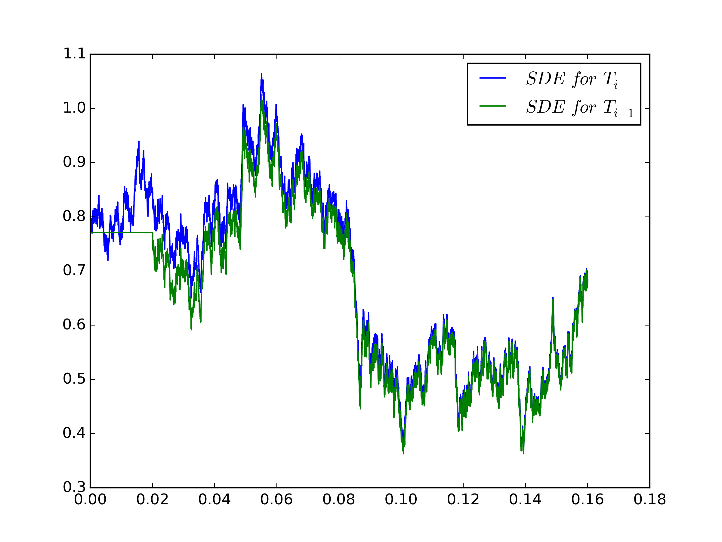
(a) Correct coupling.

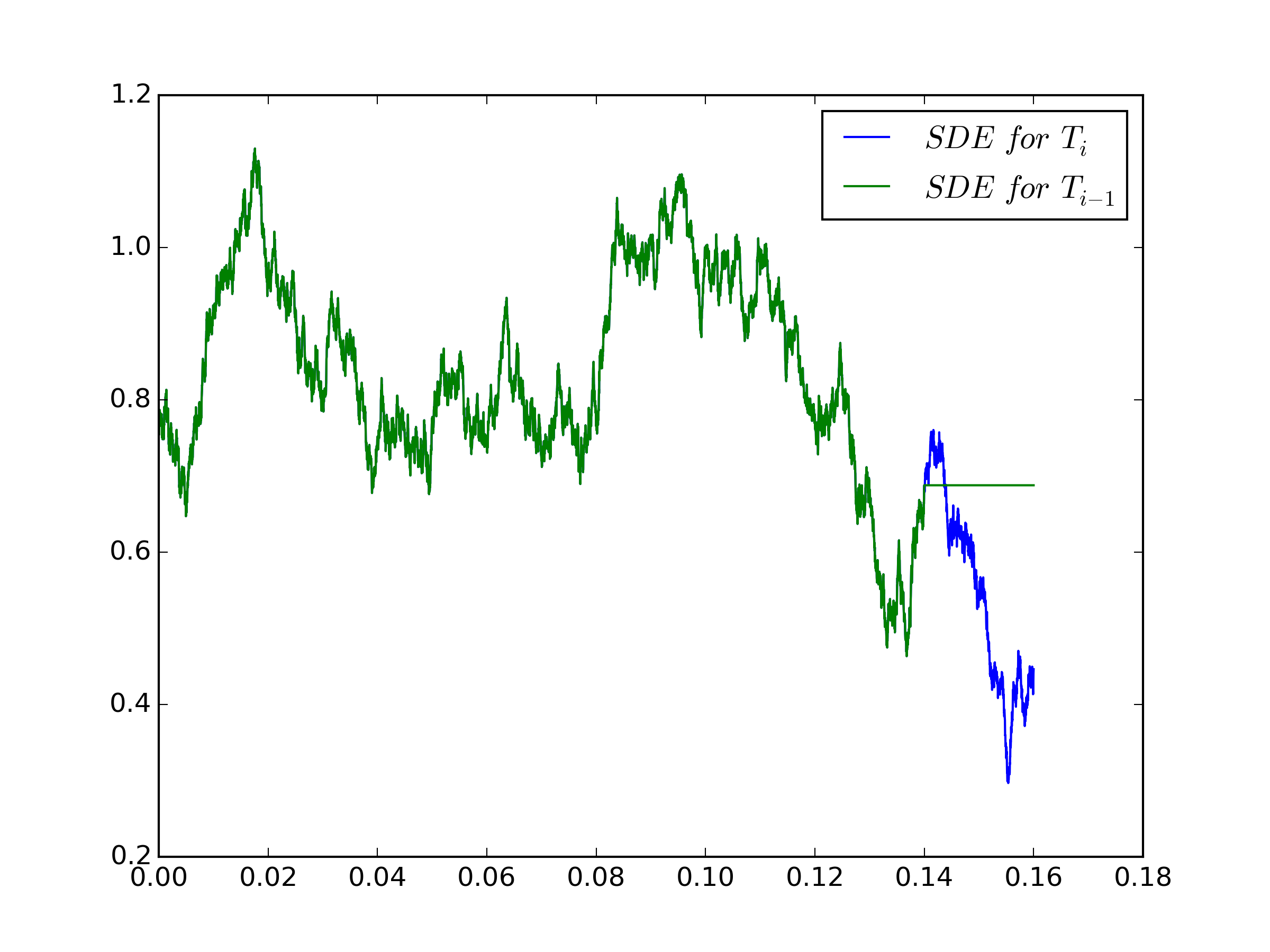
(b) Wrong coupling.

Figure 1: Shifted couplings

Let $(T_{\ell})_{\ell\leq 0}$ be an increasing sequence of positive real numbers. To couple processes with different terminal times $T_{i}$ and $T_{j}$, $i\neq j$, we exploit the time homogeneous Markov property of the flow (12). More precisely, for each $\ell\geq 0$ one would like to construct a pair $(\mathcal{X}^{(f,\ell)},\mathcal{X}^{(c,\ell)})$ of solutions to (2), which we refer to as fine and coarse paths, such that

$$\begin{split}\mathcal{L}(\mathcal{X}^{(f,\ell)}(T_{\ell-1}))&=\mathcal{L}(X_{T_{\ell}}),\\ \mathcal{L}(\mathcal{X}^{(c,\ell)}(T_{\ell-1}))&=\mathcal{L}(X_{T_{\ell-1}}),\quad\forall\ell\geq 0,\end{split}$$ (16)

and

$$\mathbb{E}|\mathcal{X}^{(f,\ell)}(T_{\ell-1})-\mathcal{X}^{(c,\ell)}(T_{\ell-1})|^{2}\leq\mathbb{E}|X_{T_{\ell}}-X_{T_{\ell-1}}|^{2}.$$ (17)

Following [26, 27, 2, 8] we propose a particular coupling denoted by $(X^{(f,\ell)},X^{(c,\ell)})$, and constructed in the following way (see also Figure 1a)

• First obtain a solution to (2) over $[0,T_{\ell}-T_{\ell-1}]$. We fix an $\mathbb{R}^{d}$-valued random variable $X(0)$ and take $X^{(f,\ell)}(0)=\psi_{0,(T_{\ell}-T_{\ell-1}),\tilde{W}}(X(0))$.

• Next couple fine and coarse paths on the remaining time interval $[0,T_{\ell-1}]$ using the same Brownian motion $W$ i.e.,

  $$X^{(f,\ell)}(T_{\ell-1})=\psi_{0,T_{\ell-1},W}(X^{(f,\ell)}(0)),$$

  and

  $$X^{(c,\ell)}(T_{\ell-1})=\psi_{0,T_{\ell-1},W}(X(0)).$$

We note here that $\nabla U(\cdot)$ in (2) is time homogenous, hence the same applies for the corresponding transition kernel $\mathcal{L}(\psi_{0,t,W}(x))=P_{t}(x,\cdot)$, which implies that condition (16) holds. Now Theorem 2.2 yields

$$\mathbb{E}|X^{(f,\ell)}(T_{\ell-1})-X^{(c,\ell)}(T_{\ell-1})|^{2}\leq\mathbb{E}|X^{(f,\ell)}(0)-X(0)|^{2}e^{-2mT_{\ell-1}}.$$ (18)

implying that condition (17) is also satisfied. We now take $\rho>1$ and define

$$T_{\ell}:=\frac{\log{2}}{2m}\rho(\ell+1)\quad\forall\ell\geq 0.$$ (19)

In our case $g_{\ell}^{(i,\ell)}=g((X^{(f,\ell)}(T_{\ell-1}))^{(i)})$ and $g_{\ell-1}^{(i,\ell)}=g((X^{(c,\ell)}(T_{\ell-1}))^{(i)})$ and we assume that $g$ is globally Lipschitz with Lipschitz constant $K$. Hence

$$\mathbb{E}|g(X^{(f,\ell)}(T_{\ell-1}))-g(X^{(c,\ell)}(T_{\ell-1}))|^{2}\leq K^{2}\mathbb{E}|X^{(f,\ell)}(T_{\ell-1})-X^{(c,\ell)}(T_{\ell-1})|^{2}$$

$$\leq K^{2}\mathbb{E}|X^{(f,\ell)}(0)-X(0)|^{2}e^{-2mT_{\ell-1}}$$

$$\leq K^{2}\mathbb{E}|X^{(f,\ell)}(0)-X_{0}|^{2}2^{-\rho\ell}$$

$$\leq K^{2}C|T_{\ell}-T_{\ell-1}|2^{-\rho\ell}.\quad\forall i\geq 0,$$

where the last inequality follows from (15).

3 MLMC in $T$ for approximation of SDEs

Having described a coupling algorithm with good contraction properties, we now present the main algorithm in Section 3.1, while in Section 3.2 we present a general numerical analysis framework for proving the convergence of our algorithm.

3.1 Description of the general algorithm

We now focus on the numerical discretisation of the Langevin equation (2). In particular, we are interested in coupling the discretisations of (2) based on step size $h_{\ell}$ and $h_{\ell-1}$ with $h_{\ell}=h_{0}2^{-\ell}$. Furthermore, as we are interested in computing expectations with respect to the invariant measure $\pi(dx)$ we also increase the time endpoint $T_{\ell}\uparrow\infty$ which is chosen such that $\frac{T_{\ell}}{h_{0}},\frac{T_{\ell}}{h_{\ell}}\in\mathbb{N}$. We illustrate the main idea using two generic discrete time stochastic processes $(x_{k})_{k\in\mathbb{N}},(y_{k})_{k\in\mathbb{N}}$ which can be defined as

$$x_{k+1}=S^{f}_{h,\xi_{k}}(x_{k}),\quad y_{k+1}=S^{c}_{h,\tilde{\xi}_{k}}(y_{k}),$$ (20)

where $S_{h,\xi_{k}}(x_{k})=S(x_{k},h,\xi_{k})$ and the operators $S^{f},S^{c}:\mathbb{R}^{d}\times\mathbb{R}_{+}\times\mathbb{R}^{d\times m}\rightarrow\mathbb{R}^{d}$ are Borel measurable, whereas $\xi,\tilde{\xi}$ are random inputs to the algorithms. The operators $S^{f}$ and $S^{c}$ in (20) need not be the same. This extra flexibility allows analysing various coupling ideas.

For example for the Euler discretisation we have

$$S_{h,\xi}(x)=x+h\nabla U(x)+\sqrt{2h}\xi,$$

where $\xi\sim\mathcal{N}(0,I)$. We will also use the notation $P_{h}(x,\cdot)=\mathcal{L}\left(S_{h,\xi}(x)\right)$ for the corresponding Markov kernel.

For MLMC algorithms one evolves both fine and coarse paths jointly, over a time interval of length $T_{\ell-1}$, by doing two steps for the finer level (with the time step $h_{\ell}$) and one on the coarser level (with the time step $h_{\ell-1}$). We will use the notation $(x^{f}_{\cdot}),(x^{c}_{\cdot})$ for

$$x_{k+\frac{1}{2}}^{f} =S_{\frac{h}{2},\xi_{k+\frac{1}{2}}}^{f}\left(x_{k}^{f}\right),\quad x_{k+1}^{f}=S_{\frac{h}{2},\xi_{k+1}}^{f}\left(x_{k+\frac{1}{2}}^{f}\right)$$ (21)

$$x_{k+1}^{c} =S_{h,\tilde{\xi}_{k+1}}^{c}(x_{k}^{c}).$$ (22)

The algorithm generating $(x^{f}_{k})_{k\in\mathbb{N}/2}$ and $(x^{c}_{k})_{k\in\mathbb{N}}$ is presented in Algorithm 1.

1. Set $x_{0}^{(f,\ell)}=x_{0}$, then simulate according to $P_{h_{\ell}}(x_{0},\cdot)$ up to time $\frac{T_{\ell}-T_{\ell-1}}{h_{\ell}}$, thus obtaining $x_{\frac{T_{\ell}-T_{\ell-1}}{h_{\ell}}}^{(f,\ell)}$;

2. Set $x_{0}^{(c,\ell)}=x_{0}$ and $x_{0}^{(f,\ell)}=x_{\frac{T_{\ell}-T_{\ell-1}}{h_{\ell}}}^{(f,\ell)}$, then simulate $(x_{\cdot}^{(f,\ell)},x_{\cdot}^{(c,\ell)})$ jointly as

   $$\textstyle\left(x_{k+1}^{(f,\ell)},x_{k+1}^{(c,\ell)}\right)=\Big{(} S^{f}_{h_{\ell},\xi_{k+1}}\circ S^{f}_{h_{\ell},\xi_{k+\frac{1}{2}}}(x_{k}^{(f,\ell)}),S^{c}_{h_{\ell-1},\frac{1}{\sqrt{2}}\left(\xi_{k+\frac{1}{2}}+\xi_{k+1}\right)}(x_{k}^{(c,\ell)})\Big{)}.$$

3. Set $k_{\ell}:=\frac{T_{\ell-1}}{h_{\ell-1}}$ and

   $$\Delta^{(i)}_{\ell}:=g\left(\left(x_{k_{\ell}}^{(f,\ell)}\right)^{(i)}\right)-g\left(\left(x_{k_{\ell}}^{(c,\ell)}\right)^{(i)}\right)$$

Algorithm 1 Coupling Langevin discretisations for $T_{\ell}\uparrow\infty$.

3.2 General convergence analysis

We will now present a general theorem for estimating the bias and the variance in the MLMC set up. We refrain from prescribing the exact dynamics of $(x_{k})_{k\geq 0}$ and $(y_{k})_{k\geq 0}$ in (20), as we seek general conditions allowing the construction of uniform in time approximations of (2) in the $L^{2}$-Wasserstein norm. The advantage of working in this general setting is that if we wish to work with more advanced numerical schemes than the Euler method (e.g. implicit, projected, adapted or randomised scheme) or general noise terms (e.g. $\alpha$-stable processes), it will be sufficient to verify relatively simple conditions to see the performance of the complete algorithm. To give the reader some intuition behind the abstract assumptions, we discuss the specific methods in Section 4.

3.2.1 Uniform estimates in time

Definition 3.1 (Bias).

We say that a process $(x_{k})_{k\in\mathbb{N}}$ converges weakly uniformly in time with order $\alpha>0$ to the solution $(X_{t})_{t\geq 0}$ of the SDE (2), if there exists a constant $c>0$ such that for any $h>0$,

$$\sup_{t\geq 0}|\mathbb{E}[g(X_{t})]-\mathbb{E}[g(x_{\lfloor t/h\rfloor})]|\leq ch^{\alpha}\,\quad g\in C^{r}_{K}(\mathbb{R})\,.$$

We define MLMC variance as follows.

Definition 3.2 (MLMC variance).

Let the operators in (21)-(22) satisfy that for all $x$

$$\mathcal{L}\left(S^{f}_{h,\xi}(x)\right)=\mathcal{L}\left(S_{h,\tilde{\xi}}^{c}(x)\right).$$ (23)

We say that the MLMC variance is of order $\beta>0$ if there exists a constant $c_{V}>0$ s.t. for any $h>0$,

$$\sup_{t\geq 0}\mathbb{E}|g(x^{c}_{\lfloor t/h\rfloor})-g(x^{f}_{\lfloor t/h\rfloor})|^{2}\leq c_{V}h^{\beta}.$$ (24)

3.2.2 Statement of sufficient conditions

We now discuss the necessary conditions imposed on a generic numerical method (20) to estimate MLMC variance. We decompose the global error into the one step error and the regularity of the scheme. To proceed we introduce the notation $x^{h}_{k,x_{s}}$ for the process at time $k$ with initial condition $x_{s}$ at time $s<k$. If it is clear from the context what initial condition is used we just write $x^{h}_{k}$. We also define the conditional expectation operator as $\mathbb{E}_{n}[\cdot]:=\mathbb{E}[\cdot|\mathcal{F}_{n}]$, where $\mathcal{F}_{n}:=\sigma\left(x^{h}_{k}:k\leq n\right)$ .

We now have the following definition.

Definition 3.3 ($L^{2}$- regularity).

We will say that the one step operator $S:\mathbb{R}^{d}\times\mathbb{R}_{+}\times\mathbb{R}^{d\times m}\rightarrow\mathbb{R}^{d}$ is $L^{2}$-regular uniformly in time if for any $\mathcal{F}_{n}$-measurable random variables $x_{n}$, $y_{n}\in\mathbb{R}^{d}$ there exist constants $K$, $C_{\mathcal{R}}$, $C_{\mathcal{H}}$, $\widetilde{\beta}>0$ and random variables $Z_{n+1}$, $\mathcal{R}_{n+1}\in\mathcal{F}_{n+1}$ and $\mathcal{H}_{n}\in\mathcal{F}_{n}$, such that for all $h\in(0,1)$

$$S_{h,\xi_{n+1}}(x_{n})-S_{h,\xi_{n+1}}(y_{n})=x_{n}-y_{n}+Z_{n+1}$$

and

$$\mathbb{E}_{n}[|S_{h,\xi_{n+1}}(x_{n})-S_{h,\xi_{n+1}}(y_{n})|^{2}] \leq(1-Kh)|x_{n}-y_{n}|^{2}+\mathcal{R}_{n}$$

$$\mathbb{E}_{n}[|Z_{n+1}|^{2}] \leq\mathcal{H}_{n}|x_{n}-y_{n}|^{2}h,$$ (25)

where

$$\begin{split}\sup_{n\geq 1}\mathbb{E}\left[\sum_{i=0}^{n-1}e^{(i-(n-1))hK/2}\mathcal{R}_{i}\right]&\leq C_{\mathcal{R}}h^{\widetilde{\beta}},\\ \sup_{n\geq 1}\mathbb{E}\left[|\mathcal{H}_{n}|^{2}\right]&\leq C_{\mathcal{H}}.\end{split}$$ (26)

We now introduce the set of the assumptions needed for the proof of the main convergence theorem.

Assumption 1.

Consider two processes $(x^{f}_{k})_{2k\in\mathbb{N}}$ and $(x^{c}_{k})_{k\in\mathbb{N}}$ obtained from the recursive application of the the operators $S^{f}_{h,\xi}(\cdot)$ and $S^{c}_{h,\xi}(\cdot)$ as defined in (20). We assume that

• There exists a constant $H>0$ such that for all $q>1$

  $$\sup_{k}\mathbb{E}|x^{f}_{k}|^{q}\leq H_{\quad}\text{and}\quad\sup_{k}\mathbb{E}|x^{c}_{k}|^{q}\leq H\,.$$

• For any $x\in\mathbb{R}^{d}$

  $$\mathcal{L}\left(S^{f}_{h,\xi}(x)\right)=\mathcal{L}\left(S_{h,\tilde{\xi}}^{c}(x)\right).$$

• The operator $S^{f}_{h,\xi}(\cdot)$ is $L^{2}$-regular uniformly in time.

Below we present the main convergence result of this section. By analogy to (21)-(22), we use the notation

$$\begin{split}x^{f}_{n,x^{c}_{n-1}}&=S^{f}_{h,\xi_{n}}\left(x^{f}_{n-\frac{1}{2},x^{c}_{n-1}}\right)\\ x^{f}_{n-\frac{1}{2},x^{c}_{n-1}}&=S^{f}_{h,\xi_{n-\frac{1}{2}}}\left(x^{c}_{n-1}\right)\\ x^{c}_{n,x^{c}_{n-1}}&=S^{c}_{h,\tilde{\xi}_{n}}\left(x^{c}_{n-1}\right)\,.\end{split}$$

Using the estimates derived here we can immediately estimate the rate of decay of MLMC variance.

Theorem 3.4.

Take $(x^{f}_{n})_{n\in\mathbb{N}/2}$ and $(x^{c}_{n})_{n\in\mathbb{N}}$ with $h\in(0,1]$ and assume that H0-H2 hold. Moreover, assume that there exist constants $c_{s}>0,c_{w}>0$ and $\alpha\geq\frac{1}{2}$, $\beta\geq 0$, $p\geq 1$ with $\alpha\geq\frac{\beta}{2}$ such that for all $n\geq 1$

$$|\mathbb{E}_{n-1}(x^{c}_{n,x^{c}_{n-1}}-x^{f}_{n,x^{c}_{n-1}})|\leq c_{w}(1+|x^{c}_{n-1}|^{p})h^{\alpha+1},$$ (27)

and

$$\mathbb{E}_{n-1}[|x^{c}_{n,x^{c}_{n-1}}-x^{f}_{n,x^{c}_{n-1}}|^{2}]\leq c_{s}(1+|x^{c}_{n-1}|^{2p})h^{\beta+1}.$$ (28)

Then the global error is bounded by

$$\mathbb{E}[|x^{c}_{T/h,x_{0}}-x^{f}_{T/h,y_{0}}|^{2}] \leq|x_{0}-y_{0}|^{2}e^{-K/2T}+2\Gamma h^{\beta}/K$$

$$+\sum_{j=0}^{n-1}e^{(j-(n-1))hK/2}\mathbb{E}(\mathcal{R}_{j})\,,$$

where $T/h=n$ and $\Gamma$ is given by (29).

Proof.

We begin using the following identity

$$x^{c}_{n,x_{0}}-x^{f}_{n,y_{0}}= x^{c}_{n,x^{c}_{n-1}}-x^{f}_{n,x^{f}_{n-1}}$$

$$= (x^{c}_{n,x^{c}_{n-1}}-x^{f}_{n,x^{c}_{n-1}})+(x^{f}_{n,x^{c}_{n-1}}-x^{f}_{n,x^{f}_{n-1}}).$$

We will be able to deal with the first term in the sum by using equations (27) and (28), while the second term will be controlled because of the $L^{2}$ regularity of the numerical scheme. Indeed, by squaring both sides in the equality above we have

$$|x^{c}_{n,y_{0}}-x^{f}_{n,x_{0}}|^{2}=|x^{c}_{n,x^{c}_{n-1}}-x^{f}_{n,x^{c}_{n-1}}|^{2}+|x^{f}_{n,x^{c}_{n-1}}-x^{f}_{n,x^{f}_{n-1}}|^{2}+2\langle x^{c}_{n,x^{c}_{n-1}}-x^{f}_{n,x^{c}_{n-1}},x^{c}_{n-1}-x^{f}_{n-1}+Z_{n}\rangle\,,$$

where in the last line we have used Assumption H2. Applying conditional expectation operator to both sides of the above equality we obtain

$$\mathbb{E}_{n-1}[|x^{c}_{n,y_{0}}-x^{f}_{n,x_{0}}|^{2}] =\mathbb{E}_{n-1}[|x^{c}_{n,x^{c}_{n-1}}-x^{f}_{n,x^{c}_{n-1}}|^{2}]+\mathbb{E}_{n-1}[|x^{f}_{n,x^{c}_{n-1}}-x^{f}_{n,x^{f}_{n-1}}|^{2}]$$

$$\qquad+2\langle x^{c}_{n-1}-x^{f}_{n-1},\mathbb{E}_{n-1}[x^{c}_{n,x^{c}_{n-1}}-x^{f}_{n,x^{c}_{n-1}}]\rangle$$

$$\qquad+2\mathbb{E}_{n-1}\langle Z_{n},x^{c}_{n,x^{c}_{n-1}}-x^{f}_{n,x^{c}_{n-1}}\rangle\,.$$

Applying Cauchy-Schwarz inequality, and using the weak error estimate (27) leads to

$$\mathbb{E}_{n-1}[|x^{c}_{n,y_{0}}-x^{f}_{n,x_{0}}|^{2}] \leq\mathbb{E}_{n-1}[|x^{c}_{n,x^{c}_{n-1}}-x^{f}_{n,x^{c}_{n-1}}|^{2}]+\mathbb{E}_{n-1}[|x^{f}_{n,x^{c}_{n-1}}-x^{f}_{n,x^{f}_{n-1}}|^{2}]$$

$$\qquad+2c_{w}h^{\alpha+1}|x^{c}_{n-1}-x^{f}_{n-1}|(1+|x^{c}_{n-1}|^{p})$$

$$\qquad+2(\mathbb{E}_{n-1}[|Z_{n}|^{2}])^{1/2}(\mathbb{E}_{n-1}[|x^{c}_{n,x^{c}_{n-1}}-x^{f}_{n,x^{c}_{n-1}}|^{2}])^{1/2}.$$

By assumptions H0-H2, and the strong error estimate (28) we have

$$\mathbb{E}_{n-1}[|x^{c}_{n,y_{0}}-x^{f}_{n,x_{0}}|^{2}] \leq c_{s}(1+|x^{c}_{n-1}|^{2p})h^{\beta+1}+|x^{c}_{n-1}-x^{f}_{n-1}|^{2}(1-Kh)+\mathcal{R}_{n-1}$$

$$+2c_{w}h^{\alpha+1}|x^{c}_{n-1}-x^{f}_{n-1}|(1+|x^{c}_{n-1}|^{p})$$

$$+2\Big{(}\mathbb{E}_{n-1}[\mathcal{H}_{n}]|x^{c}_{n-1}-x^{f}_{n-1}|^{2}h\Big{)}^{1/2}\Big{(}c_{s}(1+|x^{c}_{n-1}|^{2p})h^{\beta+1}\Big{)}^{1/2}$$

$$\leq c_{s}(1+|x^{c}_{n-1}|^{2p})h^{\beta+1}+|x^{c}_{n-1}-x^{f}_{n-1}|^{2}(1-Kh)+\mathcal{R}_{n-1}$$

$$+2c_{w}h^{\alpha+1}|x^{c}_{n-1}-x^{f}_{n-1}|(1+|x^{c}_{n-1}|^{p})$$

$$+2\Big{(}|x^{c}_{n-1}-x^{f}_{n-1}|^{2}h\Big{)}^{1/2}\Big{(}c_{s}\mathbb{E}_{n-1}[\mathcal{H}_{n}(1+|x^{c}_{n-1}|^{2p})]h^{\beta+1}\Big{)}^{1/2}\,,$$

while taking expected values and applying Cauchy-Schwarz inequality and the fact that $\alpha\geq\frac{\beta}{2}$ and $h<1$ (and hence $h^{\alpha+1}\leq h^{\frac{\beta}{2}+1}$) gives

$$\mathbb{E}[|x^{c}_{n,y_{0}}-x^{f}_{n,x_{0}}|^{2}] \leq c_{s}(1+\mathbb{E}[|x^{c}_{n-1}|^{2p}])h^{\beta+1}+\mathbb{E}[|x^{c}_{n-1}-x^{f}_{n-1}|^{2}](1-Kh)+\mathbb{E}[\mathcal{R}_{n-1}]$$

$$+2\sqrt{2}c_{w}(\mathbb{E}[|x^{c}_{n-1}-x^{f}_{n-1}|^{2}h])^{1/2}(\mathbb{E}[(1+|x^{c}_{n-1}|^{2p})h^{\beta+1}])^{1/2}$$

$$+2\mathbb{E}\Big{[}|x^{c}_{n-1}-x^{f}_{n-1}|^{2}h\Big{]}^{1/2}\mathbb{E}\Big{[}c_{s}\mathcal{H}_{n-1}(1+|x^{c}_{n-1}|^{2p})h^{\beta+1}\Big{]}^{1/2}.$$

Now Young’s inequality gives that for any $\varepsilon>0$

$$\mathbb{E}[|x^{c}_{n-1}-x^{f}_{n-1}|^{2}h]^{1/2}\mathbb{E}[(1+|x^{c}_{n-1}|^{2p})h^{\beta+1}]^{1/2}\leq\varepsilon\mathbb{E}[(x^{c}_{n-1}-x^{f}_{n-1})^{2}]h+\frac{1}{4\varepsilon}\mathbb{E}[(1+|x^{c}_{n-1}|^{2p})]h^{\beta+1}$$

and

$$\mathbb{E}\Big{[}|x^{c}_{n-1}-x^{f}_{n-1}|^{2}h\Big{]}^{1/2}\mathbb{E}\Big{[}c_{s}\mathcal{H}_{n-1}(1+|x^{c}_{n-1}|^{2p})h^{\beta+1}\Big{]}^{1/2} \leq\varepsilon\mathbb{E}\Big{[}|x^{c}_{n-1}-x^{f}_{n-1}|^{2}\Big{]}h$$

$$+\frac{1}{4\varepsilon}\mathbb{E}\Big{[}c_{s}\mathcal{H}_{n-1}(1+|x^{c}_{n-1}|^{2p})\Big{]}h^{\beta+1}\,,$$

while

$$\mathbb{E}\Big{[}\mathcal{H}_{n-1}(1+|x^{c}_{n-1}|^{2p})\Big{]}\leq\frac{1}{2}\mathbb{E}\Big{[}|\mathcal{H}_{n-1}|^{2}\Big{]}+\mathbb{E}\Big{[}(1+|x^{c}_{n-1}|^{4p})\Big{]}.$$

Let $\gamma_{n}:=\mathbb{E}[|x^{c}_{n,y_{0}}-x^{f}_{n,x_{0}}|^{2}]$. Since $(1+\mathbb{E}[|x^{c}_{n-1}|^{2p}])\leq(1+\mathbb{E}[|x^{c}_{n-1}|^{4p}])$ we have

$$\gamma_{n}\leq\left(c_{s}H+\frac{2\sqrt{2}c_{w}H+c_{s}(\mathbb{E}[|\mathcal{H}_{n-1}|^{2}]+2H)}{4\varepsilon}\right)h^{\beta+1}+\mathbb{E}[\mathcal{R}_{n-1}]+\gamma_{n-1}(1-[K-(2\sqrt{2}c_{w}+2)\varepsilon]h)$$

Fix $\varepsilon=\frac{K}{2(2\sqrt{2}c_{w}+2)}$, and define

$$\Gamma:=\Bigg{(}c_{s}H+(2\sqrt{2}c_{w}+2)\\ \times\frac{(2\sqrt{2}c_{w}H+c_{s}(\mathbb{E}[\sup_{n}|\mathcal{H}_{n-1}|^{2}]+2H))}{2K}\Bigg{)}.$$ (29)

We have

$$\gamma_{n}\leq\left(1-Kh/2\right)\gamma_{n-1}+\Gamma h^{\beta+1}+\mathbb{E}[\mathcal{R}_{n-1}].$$ (30)

We complete the proof by Lemma 3.5 below. $\square$

Lemma 3.5.

Let $a_{n},g_{n},c\geq 0$, $n\in\mathbb{N}$ be given. Moreover, assume that $1+\lambda>0$. Then, if $a_{n}\in\mathbb{R}$, $n\in\mathbb{N}$, satisfies

$$a_{n+1}\leq a_{n}(1+\lambda)+g_{n}+c,\quad n\geq 0\,,$$

then

$$a_{n}\leq a_{0}e^{n\lambda}+c\frac{e^{n\lambda}-1}{\lambda}+\sum_{j=0}^{n-1}g_{j}e^{((n-1)-j)\lambda},\qquad n\geq 1\,.$$

Remark 3.6.

Note that if we can choose $\widetilde{\beta}>\beta$ in (26) (which, as we will see in Section 4, is the case e.g. for Euler and implicit Euler schemes) then from Theorem 3.4 we get

$$\mathbb{E}[|x^{c}_{T/h,x_{0}}-x^{f}_{T/h,y_{0}}|^{2}]\leq|x_{0}-y_{0}|^{2}e^{-K/2T}+(2\Gamma/K+C_{\mathcal{R}})h^{\beta}\,.$$

3.2.3 Optimal choice of parameters

Theorem 3.4 is fundamental in terms of applying the MLMC as it guarantees that the estimate for the variance in (7) holds. In particular, we have the following Lemma.

Lemma 3.7.

Assume that all the assumptions from Theorem 3.4 hold. Let $g(\cdot)$ be a Lipschitz function. Define

$$h_{\ell}=2^{-\ell},\quad T_{\ell}\sim-\frac{2\beta}{K}\left(\log{h_{0}}+\ell\log{2}\right),\quad\forall\ell\geq 0.$$

Then resulting MLMC variance is given by.

$$\text{Var}[\Delta_{\ell}]\leq 2^{-\beta\ell},\quad\Delta_{\ell}=g\left(x_{\frac{T_{\ell-1}}{h_{\ell-1}}}^{(f,\ell)}\right)-g\left(x_{\frac{T_{\ell-1}}{h_{\ell-1}}}^{(c,\ell)}\right)$$

Proof.

Since $g$ is a Lipschitz function and

$$\mathbb{E}\left|x_{\frac{T_{\ell}-T_{\ell-1}}{h_{\ell}}}^{h_{\ell}}-x_{0}\right|^{2}<\infty,$$

the proof is a direct consequence of Theorem 3.4. $\square$

Remark 3.8.

Unlike in the standard MLMC complexity theorem [8] where the cost of simulating single path is of order $\mathcal{O}(h_{\ell}^{-1})$, here we have $\mathcal{O}(h_{\ell}^{-1}|\log{h_{\ell}}|)$. This is due to the fact that terminal times are increasing with levels. For the case $h_{\ell}=2^{-\ell}$ this results in cost per path $\mathcal{O}(2^{-\ell}\ell)$ and does not exactly fit the complexity theorem in [8]. Clearly in the case when MLMC variance decays with $\beta>1$ we still recover the optimal complexity of order $\mathcal{O}(\varepsilon^{-2})$. However, in the case $\beta=1$ following the proof by Giles [8] one can see that the complexity becomes $\mathcal{O}(\varepsilon^{-2}|\log{\varepsilon}|^{3})$.

Remark 3.9.

In the proof above we have assumed that $K$ is independent of $h$, while we have also used crude bounds in order not to deal directly with all the individual constants, since these would be dependent on the numerical schemes used.

Example 3.10.

In the case of the Euler-Maruyama method as we see from the analysis in Section 4.1 $K=2m^{\prime}-L^{2}h_{\ell},\beta=2$, while $\mathcal{R}_{n}=0,\mathcal{H}_{n}=L$. Here $L$ is the Lipschitz constant of the drift $\nabla U(x)$.

4 Examples of suitable methods

In this section we present two (out of many) numerical schemes that fulfil the conditions of Theorem 3.4. In particular, we need to verify that our scheme is $L^{2}$-regular in time, it has bounded numerical moments as in H0 and finally that it satisfies the one-step error estimates (27)-(28). Note that for both methods discussed in this section we verify condition (25) with $h^{2}$ instead of $h$. However, since in (25) we consider $h\in(0,1)$, both (35) and (42) imply (25).

4.1 Euler-Maruyama method

We start by considering the explicit Euler scheme

$$S_{h,\xi}^{f}(x)=x+h\nabla U(x)+\sqrt{2h}\xi,$$ (31)

while $S^{f}=S^{c}$, i.e., we are using the same numerical method for the fine and coarse paths. In order to be able to recover the integrability and regularity conditions we will need to impose further assumptions on the potential $U$. In particular, additionally to assumption HU0, we assume that

• There exists constant $L$ such that for any $x,y\in\mathbb{R}^{d}$

  $$|\nabla U(x)-\nabla U(y)|\leq L|x-y|$$

As a consequence of this assumption we have

$$|\nabla U(x)|\leq L|x|+|\nabla U(0)|$$ (32)

We can now prove the $L^{2}$-regularity in time of the scheme.

$L^{2}$- regularity

Since regularity is a property of the numerical scheme itself and it does not relate with the coupling between fine and coarse levels, for simplicity of notation we prove things directly for

$$x_{{n+1,x_{n}}}=S^{f}_{h,\xi_{n+1}}(x_{n}).$$ (33)

In particular, the following Lemma holds.

Lemma 4.1 ($L^{2}$-regularity).

Let HU0 and HU1 hold. Then the explicit Euler scheme is $L^{2}$-regular, i.e.,

$$\mathbb{E}_{n-1}[|x_{n,x_{n-1}}-x_{n,y_{n-1}}|^{2}]\leq (1-(2m-L^{2}h)h)|x_{n-1}-y_{n-1}|^{2}$$ (34)

$$\mathbb{E}_{n-1}[|Z_{n}|^{2}]\leq h^{2}L^{2}|x_{n-1}-y_{n-1}|^{2}$$ (35)

Proof.

The difference between the Euler scheme taking values $x_{n-1}$ and $y_{n-1}$ at time $n-1$ is given by

$$x_{n,x_{n-1}}-x_{n,y_{n-1}}=x_{n-1}-y_{n-1}+h(\nabla U(x_{n-1})-\nabla U(y_{n-1})).$$

This, along with HU0 and HU1 leads to

$$\mathbb{E}_{n-1}[(x_{n,x_{n-1}}-x_{n,y_{n-1}})^{2}] =|x_{n-1}-y_{n-1}|^{2}+2h\left\langle\nabla U(x_{n-1})-\nabla U(y_{n-1}),x_{n-1}-y_{n-1}\right\rangle$$

$$+|\nabla U(x_{n-1})-\nabla U(y_{n-1})|^{2}h^{2}$$

$$\leq|y_{n-1}-x_{n-1}|^{2}(1-2mh+L^{2}h^{2})$$

$$=|y_{n-1}-x_{n-1}|^{2}(1-(2m-L^{2}h)h).$$

This proves the first part of the lemma. Next, due to HU1

$$\mathbb{E}_{n-1}[|Z_{n}|^{2}]= h^{2}\mathbb{E}_{n-1}[|\nabla U(x_{n-1})-\nabla U(y_{n-1})|^{2}]\leq h^{2}L^{2}|x_{n-1}-y_{n-1}|^{2}.$$

$\square$

Integrability

In the Lipschitz case we only require mean-square integrability. This will become apparent when we analyse the one-step error and (27) and (28) will hold with $p=1$.

Lemma 4.2 (Integrability).

Let HU0 and HU1 hold. Then,

$$\mathbb{E}[|x_{n}|^{2}] \leq\mathbb{E}|x_{0}|^{2}\exp\{-(2m^{\prime}-L^{2}h)nh\}+2(b|\nabla U(0)|^{2}+h)\frac{1-\exp\{-(2m^{\prime}-L^{2}h)nh\}}{(2m^{\prime}-L^{2}h)h}$$

Proof.

We have

$$|x_{n}|^{2}=|x_{n-1}|^{2}+|\nabla U(x_{n-1})|^{2}h^{2}+2h\xi^{T}\xi+2hx^{T}_{n-1}\nabla U(x_{n-1})+\sqrt{2h}x^{T}_{n-1}\xi+\sqrt{2}h^{3/2}\xi^{T}\nabla U(x_{n-1})$$

and hence using (11)

$$\mathbb{E}|x_{n}|^{2}\leq\mathbb{E}|x_{n-1}|^{2}(1-2m^{\prime}h+L^{2}h^{2})+2b|\nabla U(0)|^{2}+2dh.$$

We can now use Lemma 3.5

$$\mathbb{E}|x_{n}|^{2} \leq\mathbb{E}|x_{0}|^{2}\exp\{-(2m^{\prime}-L^{2}h)nh\}+2(b|\nabla U(0)|^{2}+dh)\frac{1-\exp\{-(2m^{\prime}-L^{2}h)nh\}}{(2m^{\prime}-L^{2}h)h}$$

The proof for $q>2$ can be done in similar way by using the binomial theorem. $\square$

One-step errors estimates

Having proved $L^{2}$-regularity and integrability for the Euler scheme, we are now left with the task of proving inequalities (27) and (28) for Euler schemes coupled as in Algorithm 1. It is enough to prove the results for $n=1$. We note that both $x^{f}_{0}=x^{c}_{0}=x$ and we have the following Lemma.

Lemma 4.3 (One-step errors).

Let HU0 and HU1 hold. Then the weak one-step distance between Euler schemes with time steps $\frac{h}{2}$ and $h$, respectively, is given by

$$|\mathbb{E}[x^{f}_{1,x}-x^{c}_{1,x}]|\leq\frac{h^{3/2}}{2}L\left(\mathbb{E}\left[\frac{\sqrt{h}}{2}\left(L|x|+|\nabla U(0)|\right)\right]+\sqrt{\frac{2d}{\pi}}\right).$$ (36)

The one-step $L^{2}$ distance can be estimated as

$$\mathbb{E}|x^{f}_{1,x}-x^{c}_{1,x}|^{2}\leq h^{3}\frac{L^{2}}{4}\left(\frac{h}{2}(|x|^{2}+|\nabla U(0)|^{2})+d\right)$$ (37)

If in addition to HU0 and HU1, $U\in C^{3}$ and

$$|\partial^{2}U(x)|+|\partial^{3}U(x)|\leq C,\quad\forall x\in\mathbb{R}^{d},$$

then the order in $h$ of the weak error bound can be improved, i.e.,

$$|\mathbb{E}[x^{f}_{1,x}-x^{c}_{1,x}]|\leq Ch^{2}\mathbb{E}\big{[}|x|+h|x|^{2}+|\nabla U(0)|+h|\nabla U(0)|^{2}+d\big{]}.$$ (38)

Proof.

We calculate

$$x^{f}_{1,x}-x^{c}_{1,x} =x+\frac{h}{2}\nabla U(x)+\sqrt{h}\xi_{1}+\frac{h}{2}\nabla U\left(x+\frac{h}{2}\nabla U(x)+\sqrt{h}\xi_{1}\right)$$

$$+\sqrt{h}\xi_{2}-\left(x+h\nabla U(x)+\sqrt{h}\left(\xi_{1}+\xi_{2}\right)\right)$$

$$=\frac{h}{2}\nabla U\left(x+\frac{h}{2}\nabla U(x)+\sqrt{h}\xi_{1}\right)-\frac{h}{2}\nabla U(x).$$ (39)

It then follows from HU1 that

$$|\mathbb{E}[x^{f}_{1,x}-x^{c}_{1,x}]|\leq\frac{h^{3/2}}{2}L\mathbb{E}|\frac{\sqrt{h}}{2}\nabla U(x)+\xi_{1}|.$$

Furthermore, if we use (32), the triangle equality and the fact that $\mathbb{E}|\xi_{1}|=\sqrt{\frac{2d}{\pi}}$, we obtain (36). If we now assume that $U\in C^{3}$, then for $\delta_{t}=x+t(\frac{h}{2}\nabla U(x)+\sqrt{h}\xi_{1})$, $t\in[0,1]$, we write

$$\nabla U\left(x+\frac{h}{2}\nabla U(x)+\sqrt{h}\xi_{1}\right) =\nabla U(x)+\sum_{|\alpha|=1}\partial^{\alpha}\nabla U(x)\left(\frac{h}{2}\nabla U(x)+\sqrt{h}\xi_{1}\right)^{\alpha}$$

$$+\sum_{|\alpha|=2}\int_{0}^{1}(1-t)\partial^{\alpha}\nabla U(\delta_{t})\,dt\,\left(\frac{h}{2}\nabla U(x)+\sqrt{h}\xi_{1}\right)^{\alpha},$$

where we used multi-index notation. Consequently

$$\mathbb{E}\left[\nabla U\left(x+\frac{h}{2}\nabla U(x)+\sqrt{h}\xi_{1}\right)-\nabla U(x)\right]\leq Ch^{2}\mathbb{E}\left[(|x|+h|x|^{2}+|\nabla U(0)|+h|\nabla U(0)|^{2}+|\xi_{1}|^{2}|)\right],$$

which, together with $\mathbb{E}[|\xi_{1}|^{2}]=d$, gives (38). Equation (37) trivially follows from (4.1) by observing that

$$\mathbb{E}|x^{f}_{1,x}-x^{c}_{1,x}|^{2} \leq L^{2}\frac{h^{2}}{4}\mathbb{E}|\frac{h}{2}\nabla U(x)+\sqrt{h}\xi_{1}|^{2}$$

$$\leq h^{3}\frac{L^{2}}{4}\left(\frac{h}{2}(|x|^{2}+|\nabla U(0)|^{2})+d\right)$$

$\square$

Remark 4.4.

In the case of log-concave target the bias of MLMC using the Euler method can be explicitly quantified using the results from [4].

4.2 Non-Lipschitz setting

In the previous subsection we found out that in order to analyse the regularity and the one-step error of the explicit Euler approximation, we had to impose an additional assumption about $\nabla U(x)$ being globally Lipschitz. This is necessary since in the absence of this condition Euler method is shown to be transient or even divergent [28, 16]. However, in many applications of interest this is a rather restricting condition. An example of this, is the potential

$$U(x)=-\frac{x^{4}}{4}-\frac{x^{2}}{2}.$$

A standard way to deal with this is to use either an implicit scheme or specially designed explicit schemes [14, 30]. Here we will study only the case of implicit Euler.

4.2.1 Implicit Euler method

Here we will focus on the implicit Euler scheme

$$x_{n}=x_{n-1}+h\nabla U(x_{n})+\sqrt{2h}\xi_{n}$$

We will assume that Assumption HU0 holds and moreover replace HU1 with

• Let $k\geq 1$. For any $x,y\in\mathbb{R}^{d}$ there exists constant $L$ s.t

  $$|\nabla U(x)-\nabla U(y)|\leq L(1+|x|^{k-1}+|y|^{k-1})|x-y|$$

As a consequence of this assumption we have

$$|\nabla U(x)|\leq L|x|^{k}+|\nabla U(0)|$$ (40)

Integrability

Uniform in time bounds on the $p$-th moments of $x_{n}$ for all $p\geq 1$ can be easily deduced from the results in [23, 22]. Nevertheless, for the convenience of the reader we will present the analysis of the regularity of the scheme, where the effect of the implicitness of the scheme on the regularity should become quickly apparent.

$L^{2}$- regularity

Lemma 4.5 ($L^{2}$-regularity).

Let HU0 and HU1’ hold. Then an implicit Euler scheme is $L^{2}$-regular, i.e.,

$$\mathbb{E}_{n-1}[(x_{n,x_{n-1}}-x_{n,y_{n-1}})^{2}] \leq(1-2mh)(y_{n-1}-x_{n-1})^{2}+\mathcal{R}_{n-1},$$ (41)

and

$$\sum_{k=0}^{\infty}\mathcal{R}_{k}\leq 0.$$

Moreover,

$$\mathbb{E}_{n-1}[|Z_{n}|^{2}]\leq h^{2}\mathcal{H}_{n-1}|x_{n-1}-y_{n-1}|^{2}\,,$$ (42)

where $\mathcal{H}_{n-1}$ is defined by (43).

Proof.

The difference between the implicit Euler scheme taking values $x_{n-1}$ and $y_{n-1}$ time $n-1$ is given by

$$x_{n,x_{n-1}}-x_{n,y_{n-1}}=x_{n-1}-y_{n-1}+h(\nabla U(x_{n})-\nabla U(y_{n})).$$

This, along with HU0 and HU1 leads to

$$|x_{n,x_{n-1}}-x_{n,y_{n-1}}|^{2} =|x_{n-1}-y_{n-1}|^{2}+2h\left\langle\nabla U(x_{n})-\nabla U(y_{n}),x_{n}-y_{n}\right\rangle-|\nabla U(x_{n})-\nabla U(y_{n})|^{2}h^{2}$$

$$\leq|x_{n-1}-y_{n-1}|^{2}-2mh|x_{n,x_{n-1}}-x_{n,y_{n-1}}|^{2}$$

This implies

$$|x_{n,x_{n-1}}-x_{n,y_{n-1}}|^{2}\leq|x_{n-1}-y_{n-1}|^{2}\frac{1}{1+2mh}\leq|x_{n-1}-y_{n-1}|^{2}\left(1-\frac{2mh}{1+2mh}\right).$$

Next we take

$$|x_{n,x_{n-1}}-y_{n,y_{n-1}}|^{2} \leq|x_{n-1}-y_{n-1}|^{2}-2mh|x_{n}-y_{n}|^{2}$$

$$=(1-2mh)|x_{n-1}-y_{n-1}|^{2}-2mh(|x_{n}-y_{n}|^{2}-|x_{n-1}-y_{n-1}|^{2}).$$

In view of Definition 3.3 we define

$$\mathcal{R}_{k}:=-2mh(|x_{k}-y_{k}|^{2}-|x_{k-1}-y_{k-1}|^{2}),$$

and notice that

$$\sum_{k=1}^{n}\mathcal{R}_{k}=-2mh|x_{n}-y_{n}|^{2}\leq 0.$$

Hence the proof of the first statement in the Lemma is completed. Now, due to HU1’

$$|Z_{n}|^{2}=h^{2}|\nabla U(x_{n})-\nabla U(y_{n})|^{2} \leq h^{2}L^{2}(1+|x_{n}|^{k-1}+|y_{n}|^{k-1})^{2}|x_{n}-y_{n}|^{2}$$

$$\leq h^{2}\left(1-\frac{2mh}{1+2mh}\right)L^{2}(1+|x_{n}|^{k-1}+|y_{n}|^{k-1})^{2}|x_{n-1}-y_{n-1}|^{2}.$$

Observe that

$$\mathbb{E}_{n-1}[|x_{n}|^{2}] =|x_{n-1}|^{2}+\mathbb{E}_{n-1}[2h\left\langle\nabla U(x_{n}),x_{n}\right\rangle-|\nabla U(x_{n})|^{2}h^{2}]+h$$

$$\leq|x_{n-1}|^{2}-mh|x_{n}|^{2}+h(|\nabla U(0)|^{2}+1).$$

Consequently,

$$\mathbb{E}_{n-1}[|x_{n}|^{2}]= \frac{1}{1+mh}\left(|x_{n-1}|^{2}+h(|\nabla U(0)|^{2}+1)\right).$$

Similarly, it can be shown that $\mathbb{E}_{n-1}[|x_{n}|^{k}]$ can be expressed as a function of $|x_{n-1}|^{k}$ for $k>2$, cf. [23, 22]. This in turn implies that there exists a constant $C>0$ s.t.

$$\begin{split}\mathcal{H}_{n-1}&=\mathbb{E}_{n-1}\left[L^{2}\left(1-\frac{2mh}{1+2mh}\right)(1+|x_{n}|^{k-1}+|y_{n}|^{k-1})^{2}\right]\\ &\leq C(1+|x_{n-1}|^{2(k-1)}+|y_{n-1}|^{2(k-1)}).\end{split}$$ (43)

Due to uniform integrability of the implicit Euler scheme, (26) holds. $\square$

One-step errors estimates

Having established integrability, estimating the one-step error follows exactly the same line of the argument as in Lemma 4.3 and therefore we skip it.

5 MLMC for SGLD

In this section we discuss the multi-level Monte Carlo method for Euler schemes with inaccurate (randomised) drifts. Namely, we consider

$$S_{h,\xi,\tau}(x)=x+hb(x,\tau)+\sqrt{2h}\xi\,,$$ (44)

where $b:\mathbb{R}^{d}\times\mathbb{R}^{k}\to\mathbb{R}^{d}$ and an $\mathbb{R}^{k}$-valued random variable $\tau$ are such that

$$\mathbb{E}[b(x,\tau)]=\nabla U(x)\text{ for any }x\in\mathbb{R}^{d}\,.$$ (45)

Our main application to Bayesian inference will be discussed in Subsection 5.1. Let us now take a sequence $(\tau_{n})_{n=1}^{\infty}$ of mutually independent random variables satisfying (45). We assume that $(\tau_{n})_{n=1}^{\infty}$ are also independent of the i.i.d. random variables $(\xi_{n})_{n=1}^{\infty}$ with $\xi_{n}\sim\mathcal{N}(0,I)$. By analogy to the notation we used for the Euler scheme in (33), we will denote

$$\bar{x}_{n+1,\bar{x}_{n}}=S^{f}_{h,\xi_{n+1},\tau_{n+1}}(\bar{x}_{n})\,.$$ (46)

In the sequel we will perform a one-step analysis of the scheme defined in (46) by considering the random variables

$$\begin{split}\bar{x}^{f}_{1,x}&=S^{f}_{\frac{h}{2},\xi_{2},\tau^{f,2}}\circ S^{f}_{\frac{h}{2},\xi_{1},\tau^{f,1}}(x)\\ \bar{x}^{c}_{1,x}&=S^{c}_{h,\frac{1}{\sqrt{2}}\left(\xi_{1}+\xi_{2}\right),\tau^{c}}(x)\,,\end{split}$$ (47)

where $\xi_{1}$, $\xi_{2}\sim\mathcal{N}(0,I)$ and $\tau^{f,1}$, $\tau^{f,2}$ and $\tau^{c}$ are $\mathbb{R}^{k}$-valued random variables satisfying (45). In particular, $\tau^{f,1}$ and $\tau^{f,2}$ are assumed to be independent, but $\tau^{c}$ is not necessarily independent of $\tau^{f,1}$ and $\tau^{f,2}$. We note that in (47) we have coupled the noise between the fine and the coarse paths synchronously, i.e., as in Algorithm 1. One question that naturally occurs now is how one should choose to couple the random variables $\tau$ at different levels. In particular, in order for the condition with the telescopic sum to hold, one needs to have

$$\mathcal{L}\left(\tau^{f,1}\right)=\mathcal{L}\left(\tau^{f,2}\right)=\mathcal{L}\left(\tau^{c}\right).$$ (48)

We can of course just take $\tau^{c}$ independent of $\tau^{f,1}$ and $\tau^{f,2}$, but other choices are also possible, see Subsection 5.1 for the discussion in the context of the SGLD applied to Bayesian inference.

1. Set $x_{0}^{(f,\ell)}=x_{0}$, then simulate according to $S_{h_{\ell},\xi,\tau}(x)$

   for $\frac{T_{\ell}-T_{\ell-1}}{h_{\ell}}$ steps with independent random input;

2. set $x_{0}^{(c,\ell)}=x_{0}$ and $x_{0}^{(f,\ell)}=x_{\frac{T_{\ell}-T_{\ell-1}}{h_{\ell}}}^{h_{\ell}}$, then simulate $(x_{\cdot}^{(f,\ell)},x_{\cdot}^{(c,\ell)})$ jointly according to

   $$\left(x_{k+1}^{(f,\ell)},x_{k+1}^{(c,\ell)}\right)=\Big{(} S_{h_{\ell},\xi_{k,2},\tau^{f,2}_{k}}\circ S_{h_{\ell},\xi_{k,1},\tau^{f,1}_{k}}(x_{k}^{(f,\ell)}),S_{h_{\ell-1},\frac{1}{\sqrt{2}}\left(\xi_{k,1}+\xi_{k,2}\right),\tau^{c}_{k}}(x_{k}^{(c,\ell)})\Big{)}.$$

3. set $k_{\ell}:=\frac{T_{\ell-1}}{h_{\ell-1}}$ and

   $$\Delta^{(i)}_{\ell}:=g\left(\left(x_{k_{\ell}}^{(f,\ell)}\right)^{(i)}\right)-g\left(\left(x_{k_{\ell}}^{(c,\ell)}\right)^{(i)}\right)$$

Algorithm 2 Coupling SGLD for $t_{i}\uparrow\infty$.

In order to bound the global error for our algorithm, we make the following assumptions on the function $b$ in (44).

Assumption 2.

• There is a constant $\bar{L}>0$ such that for any $\mathbb{R}^{k}$-valued random variable $\tau$ satisfying (45) and for any $x$, $y\in\mathbb{R}^{d}$ we have

  $$\mathbb{E}[|b(x,\tau)-b(y,\tau)|]\leq\bar{L}|x-y|\,.$$ (49)

• There exist constants $\alpha_{c}$, $\sigma\geq 0$ such that for any $\mathbb{R}^{k}$-valued random variable $\tau$ satisfying (45) and for any $h>0$, $x\in\mathbb{R}^{d}$ we have

  $$\mathbb{E}[|b(x,\tau)-\nabla U(x)|^{2}]\leq\sigma^{2}(1+|x|^{2})h^{\alpha_{c}}\,.$$ (50)

Observe that conditions (49), (50) and Assumption HU1 imply that for all random variables $\tau$ satisfying (45) and for all $x\in\mathbb{R}^{d}$ we have

$$\mathbb{E}[|b(x,\tau)|^{2}]\leq\bar{L}_{0}(1+|x|^{2})$$ (51)

with $\bar{L}_{0}:=\sigma^{2}h^{\alpha_{c}}+2\max\left(L^{2},|\nabla U(0)|^{2}\right)$, cf. Section 2.4 in [21]. For a discussion on how to verify condition (50) for a subsampling scheme, see Example 2.15 in [21]. By following the proofs of Lemmas 4.1 and 4.2, we see that the $L^{2}$ regularity and integrability conditions proved therein hold for the randomised drift scheme given by (44) as well, under Assumptions HU0 and (49). Hence, in order to be able to apply Theorem 3.4 to bound the global error for (46), we only have to estimate the one step errors, i.e., we need to verify conditions (27) and (28) in an analogous way to Lemma 4.3 for Euler schemes.

Lemma 5.1.

Under Assumptions 2 and HU1 there is a constant $C_{1}=C_{1}(h,x)>0$ given by

$$C_{1}:=\frac{1}{4}L\bar{L}_{0}^{1/2}h^{1/2}(1+|x|^{2})^{1/2}+\frac{1}{2}L\sqrt{d}$$

such that for all $h>0$ we have

$$\mathbb{E}[\bar{x}_{1,x}^{f}-\bar{x}_{1,x}^{c}]\leq C_{1}h^{3/2}\,.$$ (52)

Moreover, under the same assumptions there is a constant $C_{2}=C_{2}(h,x)>0$ given by

$$C_{2}:=\frac{1}{4}\bar{L}^{2}\bar{L}_{0}h^{1+(1-\alpha_{c})^{+}}(1+|x|^{2})+d\bar{L}^{2}h^{(1-\alpha_{c})^{+}}+8\sigma^{2}(1+|x|^{2})h^{(\alpha_{c}-1)^{+}}$$

such that for all $h>0$ we have

$$\mathbb{E}[|\bar{x}_{1,x}^{f}-\bar{x}_{1,x}^{c}|^{2}]\leq C_{2}h^{2+\min(1,\alpha_{c})}\,.$$ (53)

Proof.

Note that we have

$$\bar{x}_{1,x}^{f}-\bar{x}_{1,x}^{c} =x+\frac{h}{2}b(x,\tau_{1}^{f})+\sqrt{h}\xi_{1}+\frac{h}{2}b\left(x+\frac{h}{2}b(x,\tau_{1}^{f})+\sqrt{h}\xi_{1},\tau_{2}^{f}\right)$$

$$+\sqrt{h}\xi_{2}-x-hb(x,\tau_{1}^{c})-\sqrt{h}(\xi_{1}+\xi_{2})$$

$$=\frac{h}{2}b(x,\tau_{1}^{f})+\frac{h}{2}b\left(x+\frac{h}{2}b(x,\tau_{1}^{f})+\sqrt{h}\xi_{1},\tau_{2}^{f}\right)-hb(x,\tau_{1}^{c})\,.$$ (54)

By conditioning on all the sources of randomness except for $\tau_{2}^{f}$ and using its independence of $\tau_{1}^{f}$ and $\xi_{1}$, we show

$$\mathbb{E}[\bar{x}_{1,x}^{f}-\bar{x}_{1,x}^{c}]\\ =\frac{h}{2}\mathbb{E}\left[\nabla U\left(x+\frac{h}{2}b(x,\tau_{1}^{f})+\sqrt{h}\xi_{1}\right)\right]-\frac{h}{2}\nabla U(x)\,.$$

Hence we have

$$\mathbb{E}[\bar{x}_{1,x}^{f}-\bar{x}_{1,x}^{c}]\leq\frac{h}{2}L\mathbb{E}\left[\left|\frac{h}{2}b(x,\tau_{1}^{f})+\sqrt{h}\xi_{1}\right|\right]$$

and thus, using (51) and Jensen’s inequality, we obtain (52). We now use (5.1) to compute

$$\mathbb{E}[|\bar{x}_{1,x}^{f}-\bar{x}_{1,x}^{c}|^{2}] =h^{2}\mathbb{E}\Big{|}\frac{1}{2}b(x,\tau^{f}_{1})+\frac{1}{2}b(x,\tau^{f}_{2})-\frac{1}{2}b(x,\tau^{f}_{2})++\frac{1}{2}b\left(x+\frac{h}{2}b(x,\tau_{1}^{f})+\sqrt{h}\xi_{1},\tau_{2}^{f}\right)-b(x,\tau_{1}^{c})\Big{|}^{2}$$

$$\leq 2h^{2}\mathbb{E}\left|\frac{1}{2}b(x,\tau^{f}_{1})+\frac{1}{2}b(x,\tau^{f}_{2})-b(x,\tau_{1}^{c})\right|^{2}$$

$$+\frac{1}{2}h^{2}\mathbb{E}\left|b\left(x+\frac{h}{2}b(x,\tau_{1}^{f})+\sqrt{h}\xi_{1},\tau_{2}^{f}\right)-b(x,\tau^{f}_{2})\right|^{2}$$ (55)

Observe now that due to condition (49) the second term above can be bounded by

$$\frac{1}{2}h^{2}\bar{L}^{2}\mathbb{E}\left|\frac{h}{2}b(x,\tau_{1}^{f})+\sqrt{h}\xi_{1}\right|^{2} \leq\frac{1}{2}h^{2}\bar{L}^{2}\left(\frac{h^{2}}{2}\mathbb{E}|b(x,\tau_{1}^{f})|^{2}+2h\mathbb{E}|\xi_{1}|^{2}\right)$$

$$\leq\frac{1}{2}h^{2}\bar{L}^{2}\left(\frac{h^{2}}{2}\bar{L}_{0}(1+|x|^{2})+2hd\right)\,,$$

where in the last inequality we used (51). Moreover, the first term on the right hand side of (5.1) is equal to

$$\begin{split}&2h^{2}\mathbb{E}\Big{|}\frac{1}{2}b(x,\tau^{f}_{1})-\frac{1}{2}\nabla U(x)+\frac{1}{2}\nabla U(x)-\frac{1}{2}b(x,\tau_{1}^{c})\\ &+\frac{1}{2}b(x,\tau^{f}_{2})-\frac{1}{2}\nabla U(x)+\frac{1}{2}\nabla U(x)-\frac{1}{2}b(x,\tau_{1}^{c})\Big{|}^{2}\\ &\leq 2h^{2}\Big{(}\mathbb{E}|b(x,\tau_{1}^{f})-\nabla U(x)|^{2}+2\mathbb{E}|b(x,\tau_{1}^{c})-\nabla U(x)|^{2}+\mathbb{E}|b(x,\tau_{2}^{f})-\nabla U(x)|^{2}\Big{)}\\ &\leq 8\sigma^{2}(1+|x|^{2})h^{2+\alpha_{c}}\,,\end{split}$$

where in the last inequality we used (50). This finishes the proof of (53). $\square$

Corollary 5.2.

If $\alpha_{c}=0$ in (50), then the Algorithm 2 based on the coupling given in Equation (47) with appropriately chosen $t_{i}$ has complexity $\varepsilon^{-2}|\log(\varepsilon)|^{3}.$ If $\alpha_{c}>0$, then the algorithm has complexity $\varepsilon^{-2}$.

Proof.

Because of Lemma 5.1 we can apply the results of Section 3.2. In particular, if we choose $T_{\ell}$ according to Lemma 3.7 we thus for $\alpha_{c}=0$ have $\beta=1$ in Theorem 3.4 and then the complexity follows from Remark 3.8. Similarly, for $\alpha_{c}>0$ we have $\beta>1$ and Remark 3.8 concludes the proof. $\square$

5.1 Bayesian inference using MLMC for SGLD

The main computational task in Bayesian statistics is the approximation of expectations with respect to the posterior. The a priori uncertainty in a parameter $x$ is modelled using a probability density $\pi_{0}(x)$ called the prior. Here we consider the case where for a fixed parameter $x$ the data $\left\{y_{i}\right\}_{i=1,\dots,N}$ is supposed to be i.i.d. with density ${\pi(y|x)}$. By Bayes’ rule the posterior is given by

$$\pi(x)\propto\pi_{0}(x)\prod_{i=1}^{N}{\pi(y_{i}|x)}\,.$$

This distribution is invariant for the Langevin equation (2) with

$$\nabla U(x)=\nabla\log{\pi_{0}}(x)+\sum_{i=1}^{N}\nabla\log{\pi(y_{i}|x)}.$$ (56)

Provided that appropriate assumptions are satisfied for $U$ we can thus use Algorithm 1 with Euler or implicit Euler schemes to approximate expectations with respect to $\pi(dx)$. For large $N$ the sum in equation (56) becomes a computational bottleneck. One way to deal with this is to replace the gradient by a lower cost stochastic approximation. In the following we apply our MLMC for SGLD framework to the recursion in Equation (4)

$$x_{k+1}=x_{k}+h\left(\nabla\log{\pi_{0}(x_{k})}+\frac{N}{s}\sum_{i=1}^{s}\nabla\log{\pi(y_{\tau_{i}^{k}}|x_{k})}\right)+\sqrt{2h}\xi_{k}\,,$$

where we take $\tau_{i}^{k}\overset{\text{i.i.d.}}{\sim}\mathcal{U}\left(\{1,\dots,N\}\right)\text{ for }i=1,\dots,s$ where by $\mathcal{U}\left(\{1,\dots,N\}\right)$ we denote the uniform distribution on $1,\dots,N$ which corresponds to sampling $s$ items with replacement from $1,\dots,N$. Notice that each step only costs $s$ instead of $N$. We make the following assumptions on the densities ${\pi(y|x)}$ and $\pi_{0}(x)$.

Assumption 3.

• Lipschitz conditions for prior and likelihood: There exist constants $L_{0}$, $L_{1}>0$ such that for all $i$, $x$, $y$

  $$|\nabla\log\pi\left(y_{i}\mid x\right)-\nabla\log\pi\left(y_{i}\mid y\right)| \leq L_{1}|x-y|$$

  $$|\nabla\log\pi_{0}\left(x\right)-\nabla\log\pi_{0}\left(y\right)| \leq L_{0}|x-y|\,.$$

• Convexity conditions for prior and likelihood: There exist constants $m_{0}\geq 0$ and $m_{y_{i}}\geq 0$ for $i=1,\dots,N$ such that for all $i$, $x$, $y$

  $$\log\pi_{0}(y) \leq\log\pi_{0}(x)+\left\langle\nabla\log\pi_{0}\left(x\right),y-x\right\rangle-\frac{m_{0}}{2}|x-y|^{2}$$

  $$\log\pi\left(y_{i}\mid y\right) \leq\log\pi\left(y_{i}\mid x\right)+\left\langle\nabla\log\pi\left(y_{i}\mid x\right),y-x\right\rangle-\frac{m_{y_{i}}}{2}|x-y|^{2}$$

  with $\inf_{i}(m_{0}+m_{y_{i}})>0.$

We note that these conditions imply that the scheme given by (47) with

$$b(x,\tau):=\nabla\log{\pi_{0}(x)}+\frac{N}{s}\sum_{i=1}^{s}\nabla\log{\pi(y_{\tau_{i}}|x)}$$

for $x\in\mathbb{R}^{d}$, $\tau\in\mathbb{R}^{s}$, satisfies Assumptions HU0, HU1 and (49). The value of the variance $\sigma$ of the estimator of the drift in (50) depends on the number of samples $s$, cf. Example 2.15 in [21].

Regarding the coupling of $\tau^{f,1}$, $\tau^{f,2}$ and $\tau^{c}$, we have several possible choices. We first take $s$ independent samples $\tau^{f,1}$ on the first fine-step and another $s$ independent samples $\tau^{f,2}$ on the second fine-step. The following three choices of $\tau^{c}$ ensure that equation (48) holds.

• an independent sample of $\left\{1,\dots,N\right\}$ without replacement denoted as $\tau^{c}_{\text{ind}}$ called independent coupling;

• a draw of $s$ samples without replacement from $(\tau^{f,1},$ $\tau^{f,2})$ denoted as $\tau^{c}_{\text{union}}$ called union coupling;

• the concatenation of a draw of $\frac{s}{2}$ samples without replacement from $\tau^{f,1}$ and a draw of $\frac{s}{2}$ samples without replacement from $\tau^{f,2}$ (provided that $s$ is even) denoted as $\tau^{c}_{\text{strat}}$ called stratified coupling.

We stress that any of these couplings can be used in Algorithm 2. The problem of coupling the random variables $\tau$ between different levels in an optimal way will be further investigated in our future work.

6 Numerical Investigations

In this section we perform numerical simulations that illustrate our theoretical findings. We start by studying an Ornstein-Uhlenbeck process in Section 6.1 using the explicit Euler method, while in Section 6.3 we study a Bayesian logistic regression model using the SGLD.

6.1 Ornstein Uhlenbeck process

We consider the SDE

$$dX_{t}=-\kappa X_{t}dt+\sqrt{2}dW_{t},$$ (57)

and its discretisation using the Euler method

$$x_{n+1}=S_{h,\xi}(x_{n}),\quad S_{h,\xi}(x)=x-h\kappa x+\sqrt{2h}\xi.$$ (58)

Equation (57) is ergodic with its invariant measure being $\mathcal{N}(0,\kappa^{-1})$. Furthermore, it is possible to show that the Euler method (58) is similarly ergodic with its invariant measure [36] being $\mathcal{N}\left(0,\frac{2}{2\kappa-\kappa^{2}h}\right)$. In Figure 2, we plot the outputs of our numerical simulations using Algorithm 1. The parameter of interest here is the variance of the invariant measure $\kappa^{-1}$ which we try to approximate for different mean square error tolerances $\varepsilon$.

More precisely, in Figure 2a we see the allocation of samples for various levels with respect to $\varepsilon$, while in Figure 2b we compare the computational cost of the algorithm as a function of the parameter $\varepsilon$. As we can see the computational complexity grows as $\mathcal{O}(\varepsilon^{-2})$ as predicted by our theory (Here $\alpha=\beta=2$ in (27) and (28)).

Finally, in Figure 2c we plot the approximation of the variance $\kappa^{-1}$ from our algorithm. Note that this coincides with the choice $g(x)=x^{2}$ since the mean of the invariant measure is 0. As we can see as $\varepsilon$ becomes smaller, even though the estimator is in principle biased we get perfect agreement with the true value of the variance.

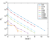
(a) Numbers of samples on different levels for given accuracy

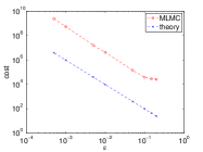
(b) Cost vs accuracy

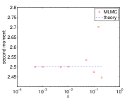
(c) Estimation of $\kappa^{-1}$

Figure 2: MLMC results for (57) for $g(x)=x^{2}$ and $\kappa=0.4$.

6.2 Non-Lipschitz

We consider the SDE

$$dX_{t}=-\left(X^{3}_{t}+X_{t}\right)dt+\sqrt{2}dW_{t},$$ (59)

and its discretisation using the implicit Euler method

$$x_{n+1}=x_{n}-h\left(x^{3}_{n+1}+x_{n+1}\right)+\sqrt{2h}\xi_{n}.$$ (60)

In Figure 3, we plot the outputs of our numerical simulations using Algorithm 1. The parameter of interest here is the second moment of the invariant measure $\int_{\mathbb{R}}x^{2}\exp\left(-\frac{1}{4}x^{4}-\frac{1}{2}x^{2}\right)dx$ which we try to approximate for different mean square error tolerances $\varepsilon$.

More precisely, in Figure 3a we see the allocation of samples for various levels with respect to $\varepsilon$, while in Figure 3b we compare the computational cost of the algorithm as a function of the parameter $\varepsilon$. As we can see the computational complexity grows as $\mathcal{O}(\varepsilon^{-2})$ as predicted by our theory (Here $\alpha=\beta=2$ in (27) and (28)).

Finally, in Figure 3c we plot the approximation of the second moment of the invariant measure from our algorithm. As we can see as $\varepsilon$ becomes smaller, even though the estimator is in principle biased we get perfect agreement with the true value of the second moment.

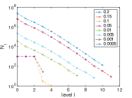
(a) Numbers of samples on different levels for given accuracy

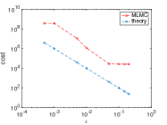
(b) Cost vs accuracy

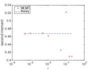
(c) Estimation of $\kappa^{-1}$

Figure 3: MLMC results for (59) for $g(x)=x^{2}$.

6.3 Bayesian logistic regression

In the following we present numerical simulations for a binary Bayesian logistic regression model. In this case the data $y_{i}\in\{-1,1\}$ is modelled by

$$p(y_{i}|\iota_{i},x)=f(y_{i}x^{t}\iota_{i})$$ (61)

where $f(z)=\frac{1}{1+\exp(-z)}\in[0,1]$ and $\iota_{i}\in\mathbb{R}^{d}$ are fixed covariates. We put a Gaussian prior $\mathcal{N}(0,C_{0})$ on $x$, for simplicity we use $C_{0}=I$ subsequently. By Bayes’ rule the posterior density $\pi(x)$ satisfies

$$\pi(x)\propto\exp\left(-\frac{1}{2}|x|_{C_{0}}^{2}\right)\prod_{i=1}^{N}f(y_{i}x^{T}\iota_{i}).$$

We consider $d=3$ and $N=100$ data points and choose the covariate to be

$$\iota=\left(\begin{array}[]{ccc}\iota_{1,1}&\iota_{1,2}&1\\ \iota_{2,1}&\iota_{2,2}&1\\ \vdots&\vdots&\vdots\\ \iota_{100,1}&\iota_{100,2}&1\end{array}\right)$$

for a fixed sample of $\iota_{i,j}\overset{\text{i.i.d.}}{\sim}\mathcal{N}\left(0,1\right)$ for $i=1,\dots,100$ and $j=1,2$.

In Algorithm 2 we can choose the starting position $x_{0}$. It is reasonable to start the path of the individual SGLD trajectories at the mode of the target distribution (heuristically this makes the distance $\mathbb{E}|x_{0}^{(c,\ell)}-x_{0}^{(f,\ell)}|$ in step 2 in Algorithm 2 small). That is we set the $x_{0}$ to be the maximum a posteriori estimator (MAP)

$$x_{0}=\text{argmax}\>\exp\left(-\frac{1}{2}|x|_{C_{0}}^{2}\right)\prod_{i=1}^{N}f(y_{i}x^{T}\iota_{i})$$

which is approximated using the Newton-Raphson method. Our numerical results are described in Figure 4. In particular, in Figure 4a we illustrate the behaviour of the coupling by plotting an estimate of the average distance during the joint evolution in step 2 of Algorithm 2. The behaviour in this figure agrees qualitatively with the statement of Theorem 3.4, as $T$ grows there is an initial exponential decay up to an additive constant. For the simulation we used $h_{0}=0.02$, $T_{\ell}=3(\ell+1)$ and $s=20$. Furthermore, in Figure 4b we plot $\text{CPU-time}\times\varepsilon^{2}$ against $\varepsilon$ for the estimation of the mean. The objective here is to estimate the mean square distance from the MAP estimator $x_{0}$ and the posterior that is $\int|x-x_{0}|^{2}\pi(x)dx$. Again, after some initial transient where $\text{CPU-time}\times\varepsilon^{2}$ decreases, we see that we get a quantitive agreement with our theory since the $\text{CPU-time}\times\varepsilon^{2}$ increases in a logarithmic way in the limit of $\varepsilon$ going to zero.

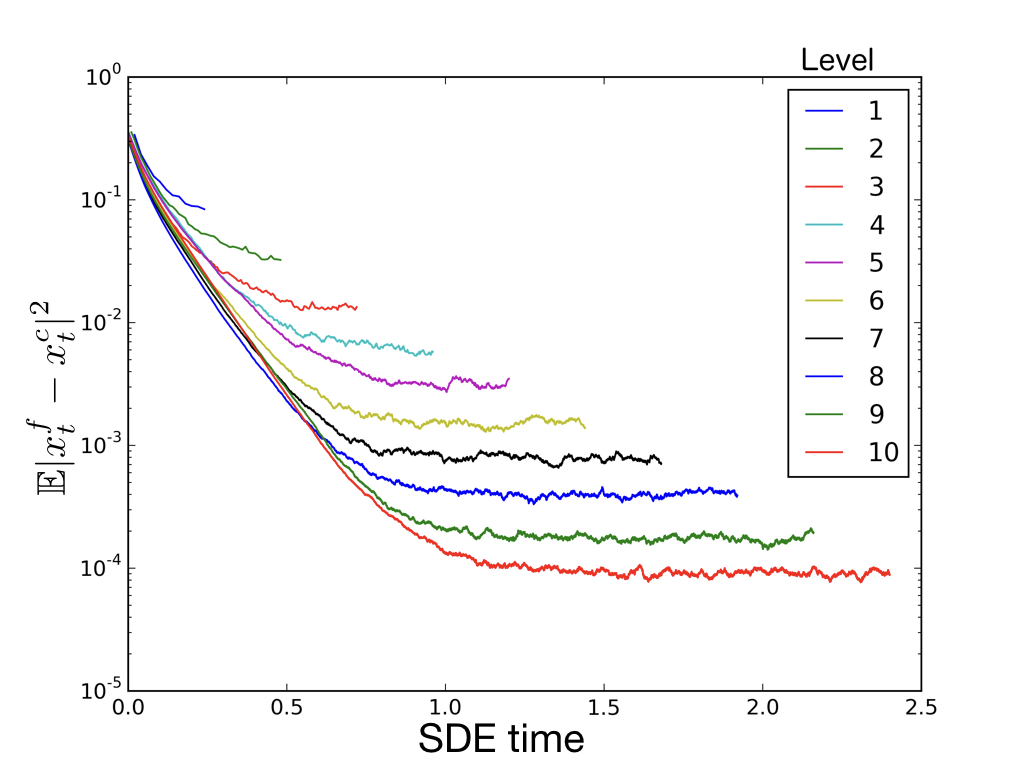
(a) Coupling difference.

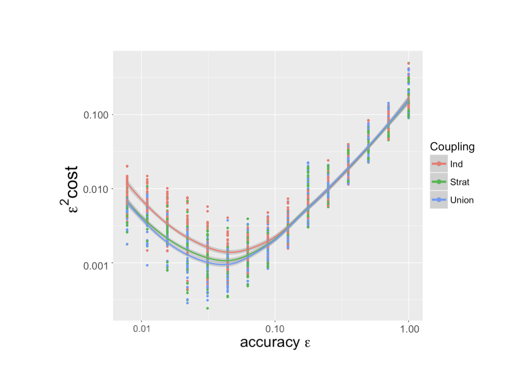
(b) Cost of MLMC.

Figure 4: (a) Illustration of the joint evolution in step 2 of Algorithm 2 for the union coupling, (b) Cost of MLMC (sequential CPU time) SGLD for Bayesian Logistic Regression for decreasing accuracy parameter $\varepsilon$ and different couplings

References

- Abdulle et al [2014] Abdulle A, Vilmart G, Zygalakis KC (2014) High order numerical approximation of the invariant measure of ergodic SDEs. SIAM J Numer Anal 52(4):1600–1622, DOI 10.1137/130935616
- Agapiou et al [2018] Agapiou S, Roberts GO, Vollmer SJ (2018) Unbiased Monte Carlo: posterior estimation for intractable/infinite-dimensional models. Bernoulli 24(3):1726–1786, DOI 10.3150/16-BEJ911
- Duffie and Glynn [1995] Duffie D, Glynn P (1995) Efficient Monte Carlo simulation of security prices. Ann Appl Probab 5(4):897–905
- Durmus and Moulines [2016] Durmus A, Moulines E (2016) High-dimensional Bayesian inference via the Unadjusted Langevin Algorithm. arXiv e-prints arXiv:1605.01559
- Fang and Giles [2016] Fang W, Giles MB (2016) Adaptive Euler-Maruyama method for SDEs with non-globally Lipschitz drift: Part i, finite time interval. arXiv preprint arXiv:160908101
- Fang and Giles [2017] Fang W, Giles MB (2017) Adaptive Euler-Maruyama method for SDEs with non-globally Lipschitz drift: Part ii, infinite time interval. arXiv preprint arXiv:170306743
- Fang and Giles [2019] Fang W, Giles MB (2019) Multilevel Monte Carlo method for ergodic SDEs without contractivity. J Math Anal Appl 476(1):149–176, DOI 10.1016/j.jmaa.2018.12.032
- Giles [2015] Giles MB (2015) Multilevel Monte Carlo methods. Acta Numer 24:259–328, DOI 10.1017/S096249291500001X
- Giles and Szpruch [2014] Giles MB, Szpruch L (2014) Antithetic multilevel Monte Carlo estimation for multi-dimensional SDEs without Lévy area simulation. Ann Appl Probab 24(4):1585–1620, DOI 10.1214/13-AAP957
- Glynn and Rhee [2014] Glynn PW, Rhee CH (2014) Exact estimation for Markov chain equilibrium expectations. J Appl Probab 51A(Celebrating 50 Years of The Applied Probability Trust):377–389, DOI 10.1239/jap/1417528487
- Hairer et al [2011] Hairer M, Mattingly JC, Scheutzow M (2011) Asymptotic coupling and a general form of Harris’ theorem with applications to stochastic delay equations. Probab Theory Related Fields 149(1-2):223–259, DOI 10.1007/s00440-009-0250-6
- Has′minskiĭ [1980] Has′minskiĭ RZ (1980) Stochastic stability of differential equations, Monographs and Textbooks on Mechanics of Solids and Fluids: Mechanics and Analysis, vol 7. Sijthoff & Noordhoff, Alphen aan den Rijn—Germantown, Md., translated from the Russian by D. Louvish
- Hastings [1970] Hastings WK (1970) Monte Carlo sampling methods using Markov chains and their applications. Biometrika 57(1):97–109, DOI 10.1093/biomet/57.1.97
- Hutzenthaler and Jentzen [2015] Hutzenthaler M, Jentzen A (2015) Numerical approximations of stochastic differential equations with non-globally Lipschitz continuous coefficients. Mem Amer Math Soc 236(1112):v+99, DOI 10.1090/memo/1112
- Hutzenthaler et al [2011] Hutzenthaler M, Jentzen A, Kloeden PE (2011) Strong and weak divergence in finite time of Euler’s method for stochastic differential equations with non-globally Lipschitz continuous coefficients. Proc R Soc Lond Ser A Math Phys Eng Sci 467(2130):1563–1576, DOI 10.1098/rspa.2010.0348
- Hutzenthaler et al [2018] Hutzenthaler M, Jentzen A, Wang X (2018) Exponential integrability properties of numerical approximation processes for nonlinear stochastic differential equations. Math Comp 87(311):1353–1413, DOI 10.1090/mcom/3146
- Kebaier [2005] Kebaier A (2005) Statistical Romberg extrapolation: a new variance reduction method and applications to option pricing. Ann Appl Probab 15(4):2681–2705, DOI 10.1214/105051605000000511
- Kloeden and Platen [1992] Kloeden P, Platen E (1992) Numerical solution of stochastic differential equations. Springer-Verlag, Berlin and New York
- Krylov [2009] Krylov NV (2009) Controlled diffusion processes, Stochastic Modelling and Applied Probability, vol 14. Springer-Verlag, Berlin, translated from the 1977 Russian original by A. B. Aries, Reprint of the 1980 edition
- Lamberton and Pagès [2002] Lamberton D, Pagès G (2002) Recursive computation of the invariant distribution of a diffusion. Bernoulli 8(3):367–405, DOI 10.1142/S0219493703000838
- Majka et al [2018] Majka MB, Mijatović A, Szpruch L (2018) Non-asymptotic bounds for sampling algorithms without log-concavity. arXiv e-prints arXiv:1808.07105
- Mao and Szpruch [2013a] Mao X, Szpruch L (2013a) Strong convergence and stability of implicit numerical methods for stochastic differential equations with non-globally Lipschitz continuous coefficients. J Comput Appl Math 238:14–28, DOI 10.1016/j.cam.2012.08.015
- Mao and Szpruch [2013b] Mao X, Szpruch L (2013b) Strong convergence rates for backward Euler-Maruyama method for non-linear dissipative-type stochastic differential equations with super-linear diffusion coefficients. Stochastics 85(1):144–171, DOI 10.1080/17442508.2011.651213
- Mattingly et al [2002] Mattingly JC, Stuart AM, Higham DJ (2002) Ergodicity for SDEs and approximations: locally Lipschitz vector fields and degenerate noise. Stochastic Process Appl 101(2):185–232, DOI 10.1016/S0304-4149(02)00150-3
- Nagapetyan et al [2017] Nagapetyan T, Duncan AB, Hasenclever L, Vollmer SJ, Szpruch L, Zygalakis K (2017) The True Cost of Stochastic Gradient Langevin Dynamics. arXiv e-prints arXiv:1706.02692
- Rhee and Glynn [2012] Rhee CH, Glynn PW (2012) A new approach to unbiased estimation for SDE’s. In: Proceedings of the Winter Simulation Conference, Winter Simulation Conference, WSC ’12, pp 17:1–17:7, URL http://dl.acm.org/citation.cfm?id=2429759.2429780
- Rhee and Glynn [2015] Rhee CH, Glynn PW (2015) Unbiased estimation with square root convergence for SDE models. Oper Res 63(5):1026–1043, DOI 10.1287/opre.2015.1404
- Roberts and Tweedie [1996] Roberts GO, Tweedie RL (1996) Exponential convergence of Langevin distributions and their discrete approximations. Bernoulli 2(4):341–363, DOI 10.2307/3318418
- Shardlow and Stuart [2000] Shardlow T, Stuart AM (2000) A perturbation theory for ergodic Markov chains and application to numerical approximations. SIAM J Numer Anal 37(4):1120–1137, DOI 10.1137/S0036142998337235
- Szpruch and Zhang [2018] Szpruch L, Zhang X (2018) -integrability, asymptotic stability and comparison property of explicit numerical schemes for non-linear SDEs. Math Comp 87(310):755–783, DOI 10.1090/mcom/3219
- Talay [2002] Talay D (2002) Stochastic Hamiltonian systems: exponential convergence to the invariant measure, and discretization by the implicit Euler scheme. Markov Process Related Fields 8(2):163–198
- Talay and Tubaro [1990] Talay D, Tubaro L (1990) Expansion of the global error for numerical schemes solving stochastic differential equations. Stochastic Anal Appl 8(4):483–509 (1991), DOI 10.1080/07362999008809220
- Teh et al [2016] Teh YW, Thiery AH, Vollmer SJ (2016) Consistency and fluctuations for stochastic gradient Langevin dynamics. J Mach Learn Res 17:Paper No. 7, 33
- Vollmer et al [2016] Vollmer SJ, Zygalakis KC, Teh YW (2016) Exploration of the (non-)asymptotic bias and variance of stochastic gradient Langevin dynamics. J Mach Learn Res 17:Paper No. 159, 45
- Welling and Teh [2011] Welling M, Teh YW (2011) Bayesian Learning via Stochastic Gradient Langevin Dynamics. In: Proceedings of the 28th ICML
- Zygalakis [2011] Zygalakis KC (2011) On the existence and the applications of modified equations for stochastic differential equations. SIAM J Sci Comput 33(1):102–130, DOI 10.1137/090762336