Theoretical and experimental study of the normal modes in a coupled two-dimensional system

Abstract

In this work, the normal modes of a two-dimensional oscillating system have been studied from a theoretical and experimental point of view. The normal frequencies predicted by the Hessian matrix for a coupled two-dimensional particle system are compared to those obtained for a real system consisting of two oscillating smartphones coupled one to the other by springs. Experiments are performed on an air table in order to remove the friction forces. The oscillation data are captured by the acceleration sensor of the smartphones and exported to file for further analysis. The experimental frequencies compare reasonably well with the theoretical predictions, specifically, within 1.7% of discrepancy.

PACS: 46.40.-f; 43.20.+g; 43.40.+s

1 Introduction

The study of the normal modes is a central issue in understanding the properties of solids and molecules, such as solid phonons and vibrations of polyatomic molecules.^{1, 2, 3, 4}. Therein, the formalism of the Hessian matrix is a common approach.⁵ Therefore, this topic is included in the courses of Physics and Chemistry degrees higher in the syllabus. For instance, the collective oscillations of a periodic solid, the phonons, which reveal important information, e.g. about thermal and electrical conductivity can be derived experimentally from neutron scattering. In the case of polyatomic molecules, normal modes are connected to the vibrational spectrum, which can be measured using a number of spectroscopic techniques. From a pedagogical point of view, the simplest classical model to characterize the vibrational modes of a polyatomic molecule is a particle system coupled by pair potentials.⁶

In general physics courses, the topic of coupled systems has been basically analyzed by means of linear 1D models.⁷ It is also possible to find a number of works in the literature on the experimental characterization of coupled 1D systems connected to external drivers ⁸, i.e. by using video-analysis techniques⁹, electromechanical systems¹⁰ or sensors.¹¹ However, when it comes to everyday life, most oscillations are more than one-dimensional. This is a good reason for including two-dimensional oscillation experiments in physics teaching.^{12, 13}

Simple experiments involving oscillations are largely facilitated by introducing smartphones as oscillating bodies in one¹⁴ and two dimensions.¹⁵ The acceleration sensor carried by these devices can be used to collect the oscillation data which can be exported to file for further analysis.¹⁶ This is a major advantage since the way of studying two-dimensional oscillations in previous work¹² was somewhat tedious. For example, the trajectory of an oscillating puck on an air table can be followed by the trace and described by it onto paper, which is later digitalized to extract the information of the trajectory¹². The introduction of the smartphone acceleration sensor to measuring this kind of two dimensional oscillations represented a major progress in our previous work¹⁵ where mechanical Lissajous figures were obtained in a very simple way.

In this work, we present an exhaustive theoretical and experimental study of the normal modes in a coupled 2D system. The experimental setup consists of two smartphones on an air table connected each other by springs and to fixed ends. The air table allows us to remove the friction forces. In these experiments the mobile phones themselves are the bodies under study. The coupled oscillations are captured with the acceleration sensors of the smartphones and the data are exported to file for further analysis.

It should be pointed out that the smartphones are just measurement tools here. Its use is not the main contribution of this work. In fact, two-dimensional oscillations could be also analyzed by using other techniques, i.e. video analysis techniques.^{9, 17}. However we have preferred to use smartphones since they allow for a fast and direct acquisition of data. Based on the collected data, the normal modes in the 2D system of coupled oscillators can be deeply analyzed, which is the main objective of this work. The theoretical frequencies derived from this analysis based on the Hessian matrix are compared with those obtained from processing the smartphone sensor data. In this way, we provide an example of physics teaching experiment on 2D coupled oscillations which contributes to fill the existing gap in the General Physics courses. In this simple way, students may be introduced to the vibrational properties of solids and molecules.

The outline of the paper is the following. In section 2, we describe the calculation of the normal modes from the Hessian matrix formalism applied to a coupled two-dimensional particle system. In section 3, experiments using two smartphones as oscillating bodies on an air table are described. The processing of the oscillation data and the comparison between the experimental and calculated normal frequencies are then presented. Finally, in section 4, some conclusions are drawn.

2 Hessian matrix formalism

A photograph of the experimental setup used for obtaining the vibrational normal modes in a coupled 2D systems is shown in Figure 1a. It consists of the air table, the air supplier, the springs, and two smartphones Samsung Galaxy S2 GT-I9100 bearing an Android version 4.03. The mass of the smartphones (plus the carrying tray) is $m$=(174.4 $\pm$ 0.1) g for both smartphones. As indicated in the figure, the lay out of the spring is a two-plus-signs geometry. The air table is a square of side (0.464$\pm$ 0.001) m. The force constant of the springs is $k$=(20.6$\pm$ 0.1) N/m and its natural length is $d$=(0.058 $\pm$0.001) m. The remaining geometric parameters of the system are shown in Figure 1b.

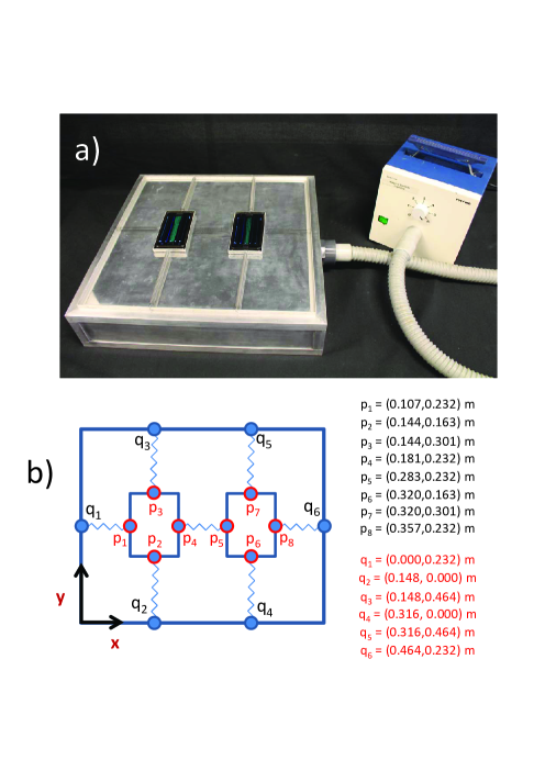
Figure 1: Photograph of the experimental setup. In panel a), a global view of the squared air table, the air supplier, the springs, and the smartphones are shown. The geometric parameters of the system at rest are shown in panel b).

First of all, the normal frequencies for the coupled system of figure 1 are calculated by a methodology based on the Hessian matrix. In this respect, the total potential energy of the system can be calculated taking into account the geometric variables defined in Figure 1b and the displacement vectors,

$$\begin{split}\Delta\overrightarrow{r_{1}}=\overrightarrow{r_{1}}-\overrightarrow{r_{1,0}}=(x_{1}-x_{1,0},y_{1}-y_{1,0}),\\ \Delta\overrightarrow{r_{2}}=\overrightarrow{r_{2}}-\overrightarrow{r_{2,0}}=(x_{2}-x_{2,0},y_{2}-y_{2,0}),\end{split}$$ (1)

where $\overrightarrow{r_{1,0}}=(x_{1,0},y_{1,0})$ and $\overrightarrow{r_{2,0}}=(x_{2,0},y_{2,0})$ are the vector positions of the smartphones at the equilibrium positions and $\overrightarrow{r_{1}}=(x_{1},y_{1})$ and $\overrightarrow{r_{2}}=(x_{2},y_{2})$ are the corresponding vector positions when the smartphones are in motion.

It should be noted that the springs stretch approximately three times their natural length. In this respect, we have made an independent experiment to check the linearity of the springs. In these conditions and considering the harmonic approximation, the total potential is given by,

$$U=\frac{k}{2}\overset{7}{\underset{i=1}{\sum}}(d_{i}-d_{0})^{2},$$ (2)

where the elongation of each spring, $d_{i}$, can be determined from the points represented in Figure 1b and from the displacements in Eq. 1,

$$\begin{split}d_{1}=|\overrightarrow{q_{1}p_{1}}+\Delta\overrightarrow{r_{1}}|,\\ d_{2}=|\overrightarrow{q_{2}p_{2}}+\Delta\overrightarrow{r_{1}}|,\\ d_{3}=|\overrightarrow{q_{3}p_{3}}+\Delta\overrightarrow{r_{1}}|,\\ d_{4}=|\overrightarrow{q_{4}p_{6}}+\Delta\overrightarrow{r_{2}}|,\\ d_{5}=|\overrightarrow{q_{5}p_{7}}+\Delta\overrightarrow{r_{2}}|,\\ d_{6}=|\overrightarrow{q_{6}p_{8}}+\Delta\overrightarrow{r_{2}}|,\\ d_{7}=|\overrightarrow{p_{4}p_{5}}+\Delta\overrightarrow{r_{2}}-\Delta\overrightarrow{r_{1}}|.\\ \end{split}$$ (3)

It should be noticed that $d_{0}$ is the natural length of the spring. Thus, at rest ($\Delta\overrightarrow{r_{1}}=\Delta\overrightarrow{r_{2}}=(0,0)$), the seven springs are elongated and the energy of the system represented by Eq.(2) is minimal but not zero.

From Figure 1, it appears that there are 6 degrees of freedom, three for the center of mass of each smartphones and $\theta$ for the rotation about the center of mass of the system. However, we have not considered rotations in our two-dimensional model consisting of two coupled particles. Under these conditions, and taking into account that oscillations take place on the x,y plane, we have a system with four degrees of freedom, namely, translations along x- and y- axes for each smartphone. The dynamical matrix (Hessian matrix)⁵ is then expressed as,

$$D_{i_{\alpha}j_{\beta}}=\frac{1}{m}\big{(}\frac{\partial^{2}U}{\partial u_{i_{\alpha}}\partial u_{j_{\beta}}}\big{)}_{u_{i_{\alpha}}=0;u_{j_{\beta}}=0},$$ (4)

where $U$ is the total potential energy and $u_{i_{\alpha}}$ ($u_{j_{\beta}}$) is the displacement of the i-th or j-th particle ($i,j=1,2$) along the $\alpha$ or $\beta$ axis ($\alpha,\beta=x,y$).

The evaluation of this matrix at the equilibrium positions and further diagonalization yields the four vibrational eigenfrequencies squared. These normal frequencies will be denoted as $\omega_{x}^{S}$, $\omega_{y}^{S}$, $\omega_{x}^{A}$, and $\omega_{y}^{A}$, corresponding to the symmetric and antisymmetric modes and for the x- and y- axes, respectively.

By using this potential energy expression, $U=U(x_{1},y_{1},x_{2},y_{2})$ given by Eq.(2), the above Hessian matrix, evaluated at the equilibrium positions is,

$$D=\left(\begin{tabular}[c]{llll}388.493&0.000&-118.119&0.0\\ 0.000&341.233&0.000&-50.953\\ -118.119&0.000&388.493&0.000\\ 0.000&-50.953&0.000&341.233\end{tabular}\right)$$ (5)

The resulting normal modes (the square root of the eigenvalues) are, $\omega_{x}^{S}=16.443$ rad/s, $\omega_{y}^{S}=17.038$ rad/s, $\omega_{x}^{A}=22.508$ rad/s, and $\omega_{y}^{A}=19.804$ rad/s. It should be noted that these values are only valid for small displacements about the equilibrium positions. It can also be noted that the eigenfrequencies obtained for the x- axis are significantly different from the ones from the 1D model, that is: $(\omega_{x}^{A})^{2}=3(\omega_{x}^{S})^{2}$. This is due to the effect of the vertical springs (p2q2, p3q3, p6q4 and p7q5) on the horizontal oscillations (for us, “horizontal” is when the oscillation is along the x- axis and “vertical” along the y- axis). In addition, and as expected, the eigenfrequencies along the y- axis also differ from the ones obtained for the x- axis. For instance, the symmetric mode along the y- axis is affected by the horizontal springs, namely, p1q1 and p8q6 (p4p5 does not stretch in this case), while the symmetric mode along the x- axis is affected by the four springs aforementioned. However, in the case of the antisymmetric mode along the y- axis, the horizontal mode p4p5 is affected.

It is also possible to perform a more exhaustive study of the normal modes of oscillation by using Newton’s second law. For example, as for the horizontal symmetric mode, the total potential given by Eq.(2) can be particularized as, $\Delta\overrightarrow{r_{1}}=\Delta\overrightarrow{r_{2}}=(\Delta x,0)$ where $\Delta x=x-x_{0}$ is a synchronized displacement of both bodies along the x- axis direction. In this situation, the potential energy only depends on the global displacement $\Delta x$. Taking into account that all involved forces are conservative, the net force acting on the system is, $\overrightarrow{F}=-\overrightarrow{\bigtriangledown}U$. For the particular case under consideration $F(x)=-dU/dx$. On the other hand, Newton’s second law can be expressed as $F(x)=m_{Total}\frac{d^{2}x}{dt^{2}}$, where $m_{Total}=2m$ is the total mass of the system. Therefore, the resulting nonlinear differential equation governing the system is,

$$-\frac{dU}{dx}=2m\frac{d^{2}x}{dt^{2}}.$$ (6)

It should be pointed out that in Eq. 6, which governs the symmetric horizontal mode, elastic forces of both horizontal and vertical springs are present. The vertical springs stretch even when the particles move along the x axis only. Contrary to a simple 1D model of coupled oscillations, there is no analytical solution of Newton’s second law for the 2D case and so a numerical solution is required.

By using the function NDSolve of the software Mathematica, Eq.6 can be solved numerically using $\Delta x_{0}$ and $\frac{dx}{dt}=0$ as initial conditions. For an initial displacement $\Delta x_{0}=0.02$ m, the numerical solution of Eq. 6 provides the trajectory displayed in Figure 2 (solid line). Additionally, the harmonic oscillation $\Delta x(t)=Acos(\omega^{S}_{x}t)$ with $A=\Delta x_{0}$ is shown in the same figure (dashed line), but it can not be seen since the curves overlap visually.

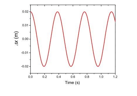
Figure 2: Simultaneous displacement of the bodies along the x axis versus time. The curves of the numerical (exact) and harmonic trajectories overlap visually.

From Figure 2, the exact period of oscillations can be determined, $T=0.3818$ s, and from it the exact (from solving Eq.6) value of the frequency, $\omega=16.457$ rad/s. The discrepancy between this value and the harmonic result ($\omega_{x}^{S}=16.443$) is only $0.09\%$. The small discrepancy between both results is due to the influence of the vertical springs. The horizontal projections of the forces exerted by these springs is linear only for small displacements. This study can be repeated for the antisymmetric mode by imposing $\Delta\overrightarrow{r_{1}}=-\Delta\overrightarrow{r_{2}}$ in the potential $U$.

A similar analysis for the symmetric and antisymmetric normal modes along the y- axis, and using $0.02$ m as initial displacement, yields discrepancies between the harmonic and the exact frequencies within 1 $\%$ in all cases. The smaller the initial displacement the smaller the discrepancy. For instance, discrepancies within 0.3 $\%$ are obtained if 1 cm is used as initial displacement. The smaller the displacements the better the harmonic approximation approaches the physical experiment. Thereby, the Hessian matrix formalism constitutes a very good approximation for obtaining the normal frequencies of a coupled 2D system in basic Physics courses.

3 Experimental setup

In order to check the normal frequencies predicted from the Hessian matrix, experiments using the experimental setup of Figure 1 are carried out. The oscillation data are captured by the acceleration sensor of the smartphones. From previous experiments, we already know that the acceleration sensor in our smartphone’s models is located at the center of the smartphone, which is coincident with the center of mass of the system.¹⁹. However, the position of the acceleration sensor may not be at the geometrical center for other models.²²

For the interaction with the mobile sensor, the free Android application “Accelerometer Toy ver 1.0.10” is used. This application takes 316 kB of SD card memory and can be downloaded from the Google play website. ¹⁸. The values of the acceleration components on $x,y$ and $z$ - axes are registered at each time step. The precision in the measurement of the acceleration is $\delta a$ = 0.03 m/s² and of time is $\delta t$ = 0.01 s. This application also allows to save the output data to file from which further analysis can be performed. Once the application is downloaded to the mobile device, a small test can be done to ensure the device is working correctly. If the mobile is left undisturbed on a horizontal surface, the application output curves for the acceleration should indicate values very close to zero for all axes. This application was successfully used in other experiments to study uniform and uniformly accelerated circular motions.¹⁹

Five experiments are performed using the setup of Figure 1. In the first four experiments, the system is set to oscillate by hand with approximately normal frequencies (symmetric and antisymmetric) along x- and y-axes, respectively. For the case of the symmetric mode, mobile phones are displaced about 1 cm towards the positive x-axis and towards the positive y- axis, respectively. For the antisymmetric mode, one of the mobile phones is displaced to the left and the other to the right for the x-axis, and downward and upward for the y-axis, respectively.

The data registered by the acceleration sensor of each smartphone for the symmetric and antisymmetric oscillations (see Figure 3) can be fitted to a harmonic function, $a(t)=A\sin(\omega t+\phi)$ where $A$ is the amplitude, $\omega$ the frequency and $\phi$ the phase. The results for the frequencies are registered in Table I. There are 8 cases in total, that is, considering each axis and each smartphone, for the symmetric and anti-symmetric modes, respectively. The graphs of the acceleration measurements and the corresponding fit curve are included in Figure 3 for each smartphone, normal mode and axis.

Table I. Frequencies and uncertainties from the fit of the acceleration data to $a(t)=A\sin(\omega t+\phi)$ along x- and y- axes for the mobiles 1 and 2, respectively.

Mobile 1 Mobile 2

$$\omega_{x}^{S}$$ (rad/s) 16.1580.016 16.2070.016

(rad/s) 16.8540.013 16.7320.010

(rad/s) 22.1580.012 22.1150.012

(rad/s) 19.9880.017 19.860 0.020

Table II. Comparison between the experimental results (average values from Table I) and those obtained from the Hessian matrix formalism.

Experimental results Hessian matrix formalism Discrepancies (%)

$$\omega_{x}^{S}$$ (rad/s) 16.18 0.03 16.443 1.6

(rad/s) 16.79 0.02 17.038 1.5

(rad/s) 22.14 0.02 22.508 1.7

(rad/s) 19.92 0.04 19.804 0.6

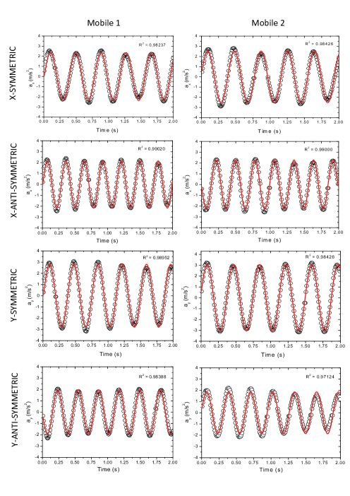
Figure 3: Symmetric and antisymmetric acceleration oscillations of the mobiles 1 and 2 along x- and y- axes respectively. The red solid lines indicate the fit. The square of the curvilinear correlation coefficient, $R^{2}$, has been included in the graphs.

The analogue values to the frequencies of the smartphones for the symmetric and antisymmetric modes and for the x- and y- axes are shown in Table II. The corresponding normal frequencies obtained from the Hessian matrix formalism are also included. A very good agreement is obtained between the experimental and the theoretical results.

Finally, in the fifth experiment, an arbitrary oscillation is started by just shifting one of the mobiles out of the equilibrium position. In this case, the arbitrary oscillation (non-normal) of the studied system can be represented as a superposition of the corresponding four normal oscillations,

$$a(t)=A_{x}^{S}\sin(\omega_{x}^{S}t+\phi_{x}^{S})+A_{x}^{A}\sin(\omega_{x}^{A}t+\phi_{x}^{A})+A_{y}^{S}\sin(\omega_{y}^{S}t+\phi_{y}^{S})+A_{y}^{A}\sin(\omega_{y}^{A}t+\phi_{y}^{A})\text{.}$$ (7)

Figure 4 shows the data points for an arbitrary oscillation. The curve fit to Eq.7 is indicated with a solid red line. The fitting to Eq. 7 has been carried out by using the non-linear fitting algorithm Levenberg-Marquardt ^{20, 21}.

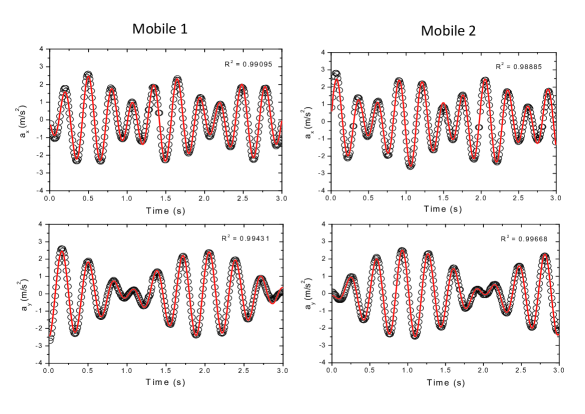
Figure 4: Free oscillations of the smartphones. The red solid lines indicate the fit.

In all cases shown in Figure 4 the values of $R^{2}$ are around 0.99 what indicates the good quality of the fitting procedure. The corresponding fitted frequencies are not shown for brevity, since they are very similar as those reported in Tables I and II. Alternatively, the main frequencies of the system can be also explored by using the Fourier transform of a free oscillation of acceleration data. Our objective was rather to prove the validity of the Hessian matrix formalism in predicting the normal frequencies of a 2D coupled system. To connect basic and simple oscillation experiments like the one in this article with this formalism helps prepare the student’s mindset for physics courses further in the syllabus.

4 Conclusions

The normal frequencies of a coupled two-dimensional system are studied both theoretically and experimentally. The normal modes were first calculated for a particle system from the Hessian matrix. An experimental setup using smartphones instead of particles and with real springs is used to test the theoretical model. The oscillation data were collected by the acceleration sensor of the smartphones. For all cases, the percentage discrepancies between the theoretical and experimental frequencies are within 1.7 %.

References

- 1 S. Jimenez, A. Pasquarello, R. Car and M. Chergui, Chem. Phys. 233 (1998) 343.
- 2 J. C. Castro-Palacios, L. Velazquez, G. Rojas-Lorenzo and J. Rubayo-Soneira, J. Mol. Struct. (Theochem) 730 (2005) 255.
- 3 J. C. Castro-Palacio, L. Vel zquez, A. Lombardi, V. Aquilanti and J. Rubayo-Soneira, J. Chem. Phys. 11126 (2007) 174701.
- 4 A. Lombardi, F. Palazzetti, G. Grossi, V. Aquilanti, J. C. Castro-Palacio and J. Rubayo-Soneira, Phys. Scr. 80 (2009) 048103.
- 5 N. W. Ashcroft and N. D. Mermin, Solid State Physics 1st edition (Saunders, Philadelphia, 1976).
- 6 E. B. Wilson Jr., J. C: Decius, P. C. Cross, Molecular Vibrations: The Theory of Infrared and Raman Vibrational Spectra (New York: Dover, 1995)
- 7 R. Resnick, D. Halliday and K. S. Krane, Physics 4th edition (Mexico, DF: CECSA, 1999)
- 8 R. Givens, D. F. de Alcantara-Bonfim and R. B. Ormond, Am. J. Phys. 71 (2003) 87.
- 9 J. A. Monsoriu, M. H. Giménez, J. Riera and A. Vidaurre, Eur. J. Phys. 26 (2005) 1149.
- 10 J. E. Molina-Coronell abnd B.P. Rodríguez-Villanueva, Rev. Mex. Fis. E 61 (2015) 65.
- 11 J. C. Castro-Palacio, L. Velázquez-Abad, F. Giménez and J. A. Monsoriu, Eur. J. Phys. 34 (2013) 737.
- 12 N. C. Bobillo-Ares and J. Fernandez-Nunez, Eur. J. Phys. 16 (1995) 223.
- 13 J. S. Pérez-Huerta, C. Meneses-Fabián and G. Rodriguez-Zurita, Rev. Mex. Fis. E 55 (2009) 8.
- 14 J. Kuhn and P. Vogt, Phys. Teach. 50 (2012) 504.
- 15 L. Tuset-Sanchis, J. C. Castro-Palacio, J. A. Gómez-Tejedor, F. J. Manjón and J. A. Monsoriu, Phys. Ed. 50 (2015) 580.
- 16 J. C. Castro-Palacio, L. Velázquez-Abad, M. H. Giménez and J. A. Monsoriu, Am. J. Phys. 81 (2013) 472.
- 17 J. Riera, J. A. Monsoriu, M. H. Giménez, J. L. Hueso and J. R. Torregrosa, Am. J. Phys. 71 (2003) 1075.
- 18 https://play.google.com/store/apps
- 19 J. C. Castro-Palacio, L. Velazquez, J. A. Gómez-Tejedor, F. J. Majón and J. A. Monsoriu, Rev. Bras. Ensino F s. 36 (2014) 2315.
- 20 K. Levenberg, Quart. Appl. Math, 2 (1944) 164.
- 21 D. Marquardt, SIAM J. Appl Math. 11 (1963) 431.
- 22 S. Mau, F. Insulla, E. E. Pickens, Z. Ding and S. C. Dudley, Phys. Teach. 54 (2016) 246.