HD 35502: a hierarchical triple system with a magnetic B5IVpe primary

Abstract

We present our analysis of HD 35502 based on high- and medium-resolution spectropolarimetric observations. Our results indicate that the magnetic B5IVsnp star is the primary component of a spectroscopic triple system and that it has an effective temperature of $18.4\pm 0.6\,{\rm kK}$, a mass of $5.7\pm 0.6\,M_{\odot}$, and a polar radius of $3.0^{+1.1}_{-0.5}\,R_{\odot}$. The two secondary components are found to be essentially identical A-type stars for which we derive effective temperatures ($8.9\pm 0.3\,{\rm kK}$), masses ($2.1\pm 0.2\,M_{\odot}$), and radii ($2.1\pm 0.4\,R_{\odot}$). We infer a hierarchical orbital configuration for the system in which the secondary components form a tight binary with an orbital period of $5.66866(6)\,{\rm d}$ that orbits the primary component with a period of over $40\,{\rm yrs}$. Least-Squares Deconvolution (LSD) profiles reveal Zeeman signatures in Stokes $V$ indicative of a longitudinal magnetic field produced by the B star ranging from approximately $-4$ to $0\,{\rm kG}$ with a median uncertainty of $0.4\,{\rm kG}$. These measurements, along with the line variability produced by strong emission in H$\alpha$, are used to derive a rotational period of $0.853807(3)\,{\rm d}$. We find that the measured $v\sin{i}=75\pm 5\,{\rm km\,s}^{-1}$ of the B star then implies an inclination angle of the star’s rotation axis to the line of sight of $24^{+6}_{-10}\degree$. Assuming the Oblique Rotator Model, we derive the magnetic field strength of the B star’s dipolar component ($14^{+9}_{-3}\,{\rm kG}$) and its obliquity ($63\pm 13\degree$). Furthermore, we demonstrate that the calculated Alfvén radius ($41^{+17}_{-6}\,R_{\ast}$) and Kepler radius ($2.1^{+0.4}_{-0.7}\,R_{\ast}$) place HD 35502’s central B star well within the regime of centrifugal magnetosphere-hosting stars.

1 Introduction

Magnetic B-type stars exhibiting strong emission (e.g. $\sigma$ Ori E, HD 142184, HD 182180, Landstreet & Borra, 1978; Grunhut et al., 2012; Rivinius et al., 2013) serve as important testbeds for understanding how stellar winds interact with magnetic fields. Models such as the Rigidly Rotating Magnetosphere (RRM) model (Townsend & Owocki, 2005) provide a qualitative description of these systems (e.g. Townsend, Owocki & Groote, 2005; Krtička et al., 2009; Oksala et al., 2010); however, detailed comparisons with observations of $\sigma$ Ori E have uncovered important discrepancies which require explanations (Oksala et al., 2012, 2015). By relaxing the RRM model’s condition that the magnetic field remains undistorted, Townsend & Owocki (2005) proposed the centrifugal breakout scenario in which the field loops episodically break and reconnect in response to an accumulating magnetospheric mass. Although magnetohydrodynamic simulations support this hypothesis (ud-Doula, Townsend & Owocki, 2006), no observational evidence of the breakout events (e.g. optical flares) has yet been reported (Townsend et al., 2013).

While these tests of the current theoretical framework provide useful information, their conclusions are based on a relatively small number of case studies. Lately, this number has been increasing as demonstrated by the recent confirmation of HD 23478’s centrifugal magnetosphere (CM) (Sikora et al., 2015), as well as the discovery of the candidate CM-host, HD 345439 (Hubrig et al., 2015). The latest addition to this particular subset of magnetic B-type stars, HD 35502, is the focus of this paper.

Over the past 60 years, the nature of HD 35502 has been redefined in various ways. Located within the Orion OB1 association (likely within the OB1a subgroup, Landstreet et al., 2007), it was initially identified as a B5V star (Sharpless, 1952; Crawford, 1958). Higher resolution spectra later obtained by Abt & Hunter (1962) revealed both narrow and broad spectral lines, the latter of which being characterized with a $v\sin{i}$ of $290\,{\rm km\,s}^{-1}$. Moreover, He i lines were reported to be relatively weak; an analysis of early-type stars within Ori OB1 carried out by Nissen (1976) demonstrated that HD 35502’s He abundance was approximately half that of the nearby chemically normal field stars. These results motivated its eventual reclassification as a B5IVsnp star (Abt & Levato, 1977).

HD 35502’s magnetic field was first detected by Borra (1981) and later confirmed by subsequent studies (Bychkov, Bychkova & Madej, 2005; Glagolevskij et al., 2010). Following the initial detection, it had been suggested that some of the unusual features apparent in its spectrum may be related to this strong field. In this paper, we use high-resolution spectra to provide a new interpretation of HD 35502 as a spectroscopic triple system whose primary component is a magnetic B-type star hosting a centrifugally supported magnetosphere.

In Section 2, we discuss both the polarized and unpolarized spectroscopic observations used in this study. Section 3 focuses on our derivation of some of the physical parameters of the system including its orbital configuration, along with the effective temperatures, surface gravities, masses, radii, and projected rotational velocities of the three stellar components. The various analytical methods used to derive these parameters, such as the modelling of spectroscopic and photometric data, are also described. In Section 4 we discuss the evidence of rotational modulation from which we derive the rotational period of HD 35502’s primary component. In Section 5, the magnetic field measurements of this component are derived along with the field geometry and strength. In Section 6, we discuss and characterize the magnetic B star’s magnetosphere. Finally, our conclusions along with our recommendations for further analytical work to be carried out are summarized in Section 8.

Table 1: ESPaDOnS and Narval spectropolarimetric observations. The SNRs per $1.8\,\text{km/s}$ pixel are reported at $5400\,{\rm\AA}$. The fifth, sixth, and seventh columns list the radial velocities of the three stellar components (see Section 3.1). The two right-most columns indicate the longitudinal magnetic field derived from H$\beta$ (see Section 5) along with the associated detection status: definite detection (DD), marginal detection (MD), and no detection (ND) as outlined by Donati et al. (1997).

HJD	Total Exp.	SNR	Instrument	$v_{r,B}$	$v_{r,A_{1}}$	$v_{r,A_{2}}$	$\langle B_{z}\rangle_{{\rm H}\beta}$	Detection
	Time (s)	(pix-1)		$({\rm km\,s}^{-1})$	$({\rm km\,s}^{-1})$	$({\rm km\,s}^{-1})$	(kG)	Status
2454702.138	1800	677	ESPaDOnS	$19.4\pm 1.3$	$55.9\pm 1.4$	$4.8\pm 2.7$	$-0.23\pm 0.19$	DD
2455849.677	3600	662	Narval	$20.0\pm 1.3$	$-15.3\pm 2.6$	$71.3\pm 1.7$	$-0.03\pm 0.16$	DD
2455893.623	3600	522	Narval	$21.2\pm 1.4$	$-5.1\pm 1.5$	$61.3\pm 2.9$	$-2.05\pm 0.20$	DD
2455910.518	3600	263	Narval	$22.7\pm 2.0$	$0.7\pm 2.0$	$55.9\pm 5.3$	$-1.30\pm 0.50$	DD
2455934.528	3600	587	Narval	$19.6\pm 1.5$	$-20.9\pm 1.1$	$76.4\pm 2.0$	$-2.12\pm 0.19$	DD
2455936.534	3600	472	Narval	$18.6\pm 1.4$	$76.5\pm 1.6$	$-19.4\pm 2.8$	$-2.32\pm 0.24$	DD
2455938.525	3600	564	Narval	$20.4\pm 1.5$	$18.1\pm 5.5$	$37.0\pm 5.9$	$0.08\pm 0.19$	ND
2455944.500	3600	494	Narval	$20.9\pm 1.4$	$1.9\pm 2.5$	$54.0\pm 2.9$	$0.16\pm 0.23$	ND
2455949.429	3600	545	Narval	$20.5\pm 1.3$	$45.4\pm 1.1$	$11.2\pm 2.5$	$-0.95\pm 0.20$	DD
2455950.472	3600	478	Narval	$21.4\pm 1.8$	$-12.5\pm 2.4$	$68.1\pm 2.9$	$-0.18\pm 0.23$	ND
2455951.471	3600	431	Narval	$22.8\pm 1.5$	$-22.6\pm 1.0$	$77.7\pm 2.0$	$-1.00\pm 0.27$	DD
2455966.376	3600	550	Narval	$19.8\pm 1.5$	$48.6\pm 1.5$	$7.5\pm 3.2$	$-1.87\pm 0.20$	DD
2455998.332	3600	397	Narval	$20.9\pm 1.4$	$53.6\pm 2.6$	$3.4\pm 3.4$	$0.28\pm 0.28$	ND
2455999.362	3600	402	Narval	$20.7\pm 1.9$	$81.8\pm 2.9$	$-25.2\pm 1.0$	$-1.64\pm 0.28$	DD
2456001.309	3600	523	Narval	$20.0\pm 1.5$	$-4.6\pm 2.4$	$60.0\pm 1.6$	$-2.39\pm 0.23$	DD
2456003.329	3600	528	Narval	$21.0\pm 1.6$	$13.5\pm 2.2$	$42.8\pm 1.9$	$0.51\pm 0.21$	DD
2456202.665	3600	604	Narval	$21.4\pm 1.3$	$65.4\pm 3.4$	$-9.4\pm 1.9$	$-2.30\pm 0.17$	DD
2456205.618	3600	494	Narval	$21.1\pm 1.5$	$-15.1\pm 2.3$	$69.5\pm 2.8$	$-0.34\pm 0.22$	DD
2456224.646	3600	450	Narval	$23.0\pm 1.3$	$27.7\pm 1.4$	$27.7\pm 1.4$	$-0.52\pm 0.24$	ND
2456246.505	3600	505	Narval	$20.5\pm 1.3$	$-15.6\pm 2.6$	$69.8\pm 1.5$	$-1.72\pm 0.22$	DD
2456293.881	1600	710	ESPaDOnS	$22.6\pm 1.4$	$79.4\pm 2.5$	$-24.9\pm 0.9$	$-1.39\pm 0.20$	DD
2456295.787	1600	190	ESPaDOnS	$21.0\pm 2.6$	$10.4\pm 1.6$	$44.1\pm 1.4$	$-3.06\pm 0.71$	ND
2456295.808	1600	231	ESPaDOnS	$22.8\pm 2.3$	$9.3\pm 1.3$	$45.2\pm 1.9$	$-2.83\pm 0.57$	MD
2456556.002	1600	582	ESPaDOnS	$24.7\pm 1.9$	$43.0\pm 1.9$	$10.8\pm 1.8$	$-1.37\pm 0.28$	DD
2456557.140	1600	670	ESPaDOnS	$19.2\pm 1.5$	$-18.2\pm 1.9$	$70.9\pm 1.6$	$-3.27\pm 0.20$	DD
2456560.077	1600	612	ESPaDOnS	$20.8\pm 1.4$	$74.5\pm 1.9$	$-20.5\pm 2.1$	$-0.05\pm 0.25$	ND

2 observations

2.1 ESPaDOnS & Narval spectropolarimetry

Spectropolarimetric observations of HD 35502 were obtained over the course of 5 years (Aug. 23, 2008 to Sept. 24, 2013) in the context of the MiMeS (Wade et al., 2015) and BinaMIcS (Alecian et al., 2015) surveys. Nineteen Stokes $V$ observations were obtained using the high-resolution ($R\simeq 65\,000$) spectropolarimeter Narval installed at the Télescope Bernard Lyot (TBL) over a wavelength range of approximately $3\,600-10\,000\,{\rm\AA}$. Ten Stokes $V$ spectra were also obtained using the twin instrument ESPaDOnS installed at the Canada-France-Hawaii Telescope (CFHT). Three of these observations exhibited signal-to-noise ratios (SNRs) $\lesssim 100$ and were removed from the analysis. A median SNR of $522$ was obtained from the twenty six observations. Both the ESPaDOnS and Narval observations were reduced using the Libre-ESpRIT pipeline (Donati et al., 1997) yielding final Stokes $I$ and $V$ spectra (for a detailed description of the reduction procedure, see e.g. Silvester et al., 2012). The Heliocentric Julian Dates (HJDs), total exposure times, and SNRs are listed in Table 1.

2.2 dimaPol spectropolarimetry

Twenty-four medium-resolution spectropolarimetric observations were obtained with dimaPol ($R\simeq 10\,000$) installed at the Dominion Astrophysical Observatory (DAO) (Monin et al., 2012) from Feb. 7, 2009 to Feb. 15, 2012. Two of these observations had SNRs $\lesssim 100$ and were removed from the analysis. The remaining twenty-two Stokes $V$ observations of H$\beta$ were used to derive longitudinal field measurements; the HJDs, exposure times, SNRs, and longitudinal field measurements are listed in Table 2.

2.3 FEROS spectroscopy

Thirty-two unpolarized spectra were acquired from Dec. 30, 2013 to Jan. 3, 2014 using the spectrograph FEROS mounted on the $2.2\,{\rm m}$ MPG/ESO telescope located at La Silla Observatory. The instrument has a resolving power of $R=48\,000$ across a wavelength range of $3\,600-9\,200\,\rm{\AA}$ (Kaufer et al., 1999). The spectra were reduced using the FEROS Data Reduction System. The pipeline automatically carries out bias subtraction, flat fielding, and extraction of the spectral orders; wavelength calibration is carried out using ThAr and ThArNe lamps. Uncertainties in the measured intensities were estimated from the root mean square (RMS) of the continuum intensity at multiple points throughout each spectrum (e.g. Wade et al., 2012). The HJDs, total exposure times, and SNRs are listed in Table 3.

2.4 H$\alpha$ spectroscopy

A total of 131 spectroscopic observations of H$\alpha$ covering various wavelength ranges from approximately $6\,300-6\,800\,{\rm\AA}$ are also used in this study. One hundred thirteen of these observations were obtained at the DAO from Nov. 26, 1991 to Feb. 4, 2012. Seven of the spectra were removed from the analysis on account of their SNRs being $\lesssim 50$. Both the McKellar spectrograph installed at the $1.2\,{\rm m}$ Plaskett telescope and the spectrograph mounted at the Cassegrain focus of DAO’s $1.8\,{\rm m}$ telescope were used to acquire the spectra.

The remaining eleven observations were obtained at CFHT from Nov. 21, 1991 to Oct. 3, 1995 using the now decommissioned Coudé f/8.2 spectrograph.

2.5 $uvby$ photometry

149 $uvby$ photometric measurements were obtained from Jan. 27, 1992 to Mar. 13, 1994 using the $0.75\,{\rm m}$ Four College Automated Photoelectric Telescope (FCAPT) on Mt. Hopkins, AZ. The dark count was first measured and then in each filter the sky-ch-c-v-c-v-c-v-c-ch-sky counts were obtained, where sky is a reading of the sky, ch that of the check star, c that of the comparison star, and v that of the variable star. No corrections have been made for neutral density filter differences among each group of variable, comparison, and check stars. HD 35575 was the comparison and HD 35008 the check (i.e. second comparison) star. The standard deviations of the ch-c values were 0.006 mag, except for u for which it was 0.008 mag. We adopted uncertainties of 0.005 mag for each measurement based on the highest precision typically achieved with FCAPT. Table HD 35502: a hierarchical triple system with a magnetic B5IVpe primary contains the complete list of photometry.

Table 2: Spectropolarimetric observations of HD 35502 obtained with dimaPol. Columns $1$ to $3$ list the HJDs, exposure times, and SNRs. Column $4$ lists the longitudinal field measurements derived from the H$\beta$ Stokes $V$ profiles.

HJD	Total Exp.	SNR	$\langle B_{z}\rangle_{\rm H\beta}$
	Time (s)	(pix-1)	(kG)
2454869.764	4800	410	$-1.95\pm 0.27$
2454872.773	3600	240	$-0.64\pm 0.25$
2455109.047	5400	240	$-2.88\pm 0.51$
2455110.964	5400	260	$-1.60\pm 0.25$
2455167.855	6000	290	$-2.27\pm 0.21$
2455168.829	6000	320	$-2.21\pm 0.38$
2455169.881	7200	280	$-1.72\pm 0.43$
2455170.867	7200	190	$0.31\pm 0.31$
2455190.766	7200	230	$-2.57\pm 0.33$
2455191.781	7200	260	$-2.29\pm 0.30$
2455192.790	7200	130	$-3.95\pm 1.09$
2455193.742	7200	210	$-1.61\pm 0.33$
2455261.655	6000	290	$-2.04\pm 0.41$
2455262.685	6000	300	$-2.31\pm 0.26$
2455264.661	6000	270	$-0.89\pm 0.37$
2455580.803	6000	270	$-0.07\pm 0.38$
2455583.800	4800	140	$-2.38\pm 0.94$
2455594.711	7200	230	$-2.39\pm 0.60$
2455611.691	5700	210	$-2.07\pm 0.47$
2455904.864	6600	170	$-3.60\pm 0.56$
2455964.666	5400	190	$-2.48\pm 0.34$
2455972.644	7200	260	$0.58\pm 0.44$

3 Physical parameters

Based on the high-resolution spectra obtained of HD 35502, three distinct sets of spectral lines are apparent: the strong and broad lines associated with a hot star and two nearly identifical components attributable to two cooler stars which are observed to change positions significantly. Based on HD 35502’s reported spectral type, the bright, dominant component is presumed to be a hot B5 star (Abt & Levato, 1977); the weaker components are inferred to be two cooler A-type stars based on the presence of Fe ii lines and the absence of Fe iii lines. As will be shown in the next section, the lines of the A stars show velocity variations consistent with a binary system. Hence we conclude that HD 35502 is an SB3 system.

Some of the B star lines (the He i lines, in particular) appear to exhibit intrinsic variability. Such features are commonly found in magnetic He peculiar stars (e.g. Borra, Landstreet & Thompson, 1983; Bolton et al., 1998; Shultz et al., 2015).

3.1 Orbital solution

The radial velocity ($v_{r}$) of the central B star ($B$) in each observation was determined using spectral lines for which no significant contribution from the two A stars ($A_{1}$ and $A_{2}$) was apparent. C ii$\,\lambda 4267$ was found to be both relatively strong (with a depth of $10$ per cent of the continuum) and only weakly variable. The H$\alpha$ spectra encompassed a limited range of wavelengths with few lines from which $v_{r}$ could be accurately determined. We used C ii$\,\lambda 6578$ and He i$\,\lambda 6678$ in order to estimate $v_{r}$ from all of the spectra (spanning a $22$ year period). However, measurements made from He i$\,\lambda 6678$ were subject to systematic errors associated with strong variability (see Section 6). Moreover, the shallower depth of C ii$\,\lambda 6578$ ($<4$ per cent of the continuum) and its blending with H$\alpha$ resulted in both a decrease in precision and a larger scatter in $v_{r}$ compared with those values derived from C ii$\,\lambda 4267$.

The radial velocities were calculated by fitting a rotationally-broadened Voigt function to the C ii$\,\lambda 4267$, C ii$\,\lambda 6578$, and He i$\,\lambda 6678$ lines. The uncertainties were estimated through a bootstrapping analysis involving the set of normalized flux measurements ($I/I_{c}$) spanning each line. A random sample of 61 per cent of the data points was selected to be removed at each iteration. These points were then replaced by another set that was randomly sampled from $I/I_{c}$. The fitting routine was then repeated on this new data set. 1000 iterations of the bootstrapping routine were carried out and a probability distribution was obtained for each fitting parameter. The uncertainties in each of the fitting parameters were then taken as the $3\sigma$ standard deviations associated with each probability distribution.

The value of $v_{r}$ inferred from C ii$\,\lambda 4267$ was found to exhibit a median uncertainty of $1.5\,{\rm km\,s}^{-1}$ and a standard deviation of $1.4\,{\rm km\,s}^{-1}$. Larger uncertainties were derived using He i$\,\lambda 6678$ and C ii$\,\lambda 6578$ ranging from $1-53\,{\rm km\,s}^{-1}$. Similarly, $v_{r}$ inferred from C ii$\,\lambda 6578$ and He i$\,\lambda 6678$ yielded larger standard deviations of $9$ and $18\,{\rm km\,s}^{-1}$, respectively. In the case of He i$\,\lambda 6678$, the decrease in precision and increase in scatter relative to the more stable C ii$\,\lambda 4267$ measurements is likely the result of the intrinsic line variability. No significant $v_{r}$ variability was detected using C ii$\,\lambda 4267$ ($\langle v_{r}\rangle=21\pm 2\,{\rm km\,s}^{-1}$), C ii$\,\lambda 6578$ ($\langle v_{r}\rangle=30\pm 15\,{\rm km\,s}^{-1}$), or He i$\,\lambda 6678$ ($\langle v_{r}\rangle=30\pm 8\,{\rm km\,s}^{-1}$).

The radial velocities of the two A stars were calculated from Stokes I profiles produced using the Least Squares Deconvolution (LSD) method (Donati et al., 1997; Kochukhov, Makaganiuk & Piskunov, 2010). The LSD line mask used to carry out the procedure was compiled using data taken from the Vienna Atomic Line Database (VALD) (Kupka et al., 2000). In order to isolate the A stars from the dominant B star component in the Stokes I LSD profiles, we used a line list associated with an $8000\,{\rm K}$ star having a surface gravity of $\log{g}=4.0$ (cgs) and a microturbulence of $v_{\rm mic}=0$. Fig. 1 shows the LSD profiles generated using a different line mask in which both the A and B star components are apparent. The majority of the radial velocities were then determined by simultaneously fitting two Gaussians to the sharp components of the Stokes I profiles. In the case of the Narval observation obtained at ${\rm HJD}=2456224.646$, the sharp line profiles were completely blended and the radial velocities were estimated by fitting a single Gaussian and adopting the resultant velocity for both components. The $v_{r}$ errors were estimated using a $1000$ iteration bootstrapping analysis. We note that the contribution of the B star to the Stokes $I$ LSD profiles was generally weak; however, in certain observations, small contributions were present which resulted in small deformations in the continuum between the two A star profiles. In these cases, the A star line appearing closest to these deformations was more affected than the other A star thereby yielding slightly higher uncertainties in the fitting procedure. The values of the two A stars’ radial velocities were found to range from $-30.4$ to $78.6\,{\rm km\,s}^{-1}$ with an average uncertainty of $2.4\,{\rm km\,s}^{-1}$.

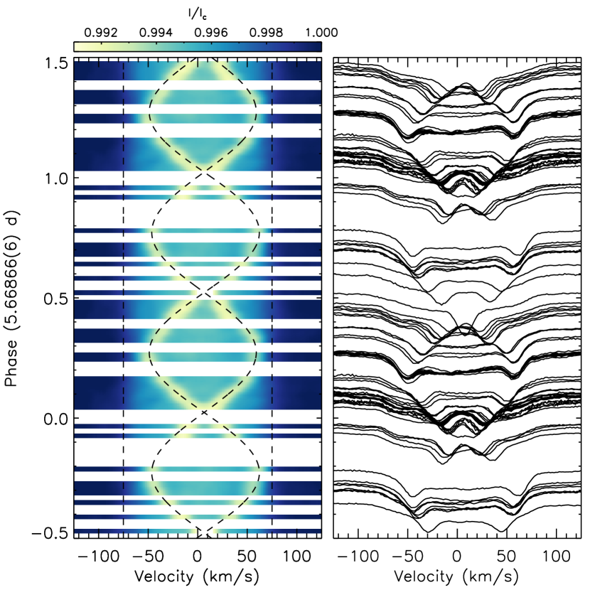
Figure 1: ESPaDOnS, Narval, and FEROS Stokes $I$ LSD profiles (right) and dynamic Stokes $I$ LSD profiles (left) generated such that the three spectral components are emphasized. The observations are phased by the A star orbital period of $5.66866(6)\,{\rm d}$. The vertical dashed black lines indicate the surface of the B star located at $v=\pm v\sin{i}=\pm 75\,{\rm km\,s}^{-1}$. The dashed black sinusoids correspond to the fits obtained for $v_{r}$ of the two A stars.

Table 3: Unpolarized spectra obtained using FEROS. The SNRs per $2.8\,{\rm km\,s}^{-1}$ pixel listed in column 3 are estimated from the RMS of the continuum near $\lambda=5400\,{\rm\AA}$. The fourth, fifth, and sixth columns list the radial velocities of the three stellar components (see Section 3.1).

HJD	Total Exp.	RMS	$v_{r,B}$	$v_{r,A_{1}}$	$v_{r,A_{2}}$
	Time (s)	SNR	$({\rm km\,s}^{-1})$	$({\rm km\,s}^{-1})$	$({\rm km\,s}^{-1})$
2456656.568	300	271	$19.5\pm 1.6$	$75.4\pm 2.4$	$-25.4\pm 1.5$
2456656.609	600	315	$20.9\pm 1.4$	$76.0\pm 2.1$	$-26.2\pm 1.1$
2456658.535	600	262	$19.2\pm 1.9$	$10.3\pm 3.1$	$39.2\pm 2.9$
2456658.542	124	145	$19.2\pm 2.7$	$10.1\pm 1.8$	$39.2\pm 1.5$
2456658.679	300	215	$20.5\pm 1.8$	$2.9\pm 1.8$	$46.5\pm 2.5$
2456658.683	300	200	$21.8\pm 1.8$	$2.8\pm 1.7$	$46.5\pm 3.0$
2456658.686	300	195	$22.3\pm 1.5$	$2.8\pm 1.7$	$46.8\pm 2.0$
2456658.690	300	178	$20.2\pm 2.0$	$2.2\pm 2.1$	$47.0\pm 2.4$
2456658.694	300	215	$20.9\pm 1.8$	$2.3\pm 2.3$	$47.2\pm 2.7$
2456658.698	300	248	$21.4\pm 1.5$	$2.1\pm 2.0$	$47.4\pm 2.9$
2456658.701	300	219	$20.4\pm 1.7$	$1.9\pm 1.8$	$47.6\pm 2.1$
2456658.702	300	181	$21.3\pm 1.6$	$1.6\pm 2.3$	$47.6\pm 1.6$
2456658.709	300	286	$21.8\pm 1.9$	$1.3\pm 1.5$	$48.1\pm 2.2$
2456658.713	300	251	$21.5\pm 3.3$	$1.3\pm 2.3$	$48.1\pm 2.4$
2456658.763	600	252	$19.7\pm 1.6$	$-1.5\pm 4.7$	$51.1\pm 2.4$
2456659.628	600	267	$18.4\pm 1.6$	$-29.3\pm 1.3$	$77.8\pm 2.3$
2456659.671	300	222	$19.1\pm 1.5$	$-29.9\pm 1.2$	$78.1\pm 1.7$
2456659.677	400	284	$19.6\pm 1.6$	$-30.1\pm 1.5$	$78.3\pm 1.8$
2456659.682	300	233	$19.9\pm 1.9$	$-30.0\pm 1.6$	$78.5\pm 2.3$
2456659.685	300	209	$19.7\pm 1.7$	$-29.8\pm 1.3$	$78.0\pm 1.6$
2456659.689	300	299	$18.8\pm 1.8$	$-29.9\pm 1.7$	$78.0\pm 1.6$
2456659.693	300	245	$17.5\pm 2.9$	$-30.3\pm 1.9$	$78.1\pm 2.0$
2456659.697	300	310	$19.9\pm 1.7$	$-30.0\pm 1.1$	$78.1\pm 1.3$
2456659.700	300	240	$20.5\pm 1.7$	$-30.1\pm 2.0$	$78.2\pm 1.8$
2456659.704	300	222	$20.4\pm 1.6$	$-30.1\pm 1.6$	$78.1\pm 1.9$
2456659.708	300	231	$20.7\pm 2.0$	$-30.2\pm 1.3$	$78.2\pm 1.3$
2456659.746	600	300	$20.5\pm 1.5$	$-29.8\pm 1.3$	$78.0\pm 1.4$
2456660.614	600	249	$20.6\pm 1.6$	$-4.4\pm 3.6$	$53.2\pm 4.3$
2456660.653	600	276	$21.6\pm 1.6$	$-2.4\pm 3.1$	$51.7\pm 4.1$
2456660.724	600	265	$21.5\pm 1.6$	$1.1\pm 2.7$	$48.1\pm 2.9$
2456660.763	600	299	$19.7\pm 1.7$	$2.8\pm 2.2$	$46.5\pm 3.1$
2456660.801	600	250	$21.5\pm 2.0$	$5.1\pm 1.9$	$43.9\pm 2.6$

The spectral characteristics of the two A-type components are nearly identical; therefore, it is not possible to unambiguously attribute a particular line profile in each spectrum to a particular star. Nevertheless, the importance of this ambiguity can be reduced by making simplifying assumptions.

First, we assumed that the two A stars are gravitationally bound and therefore orbit a common center of mass (having a radial velocity $v_{\rm cm}$) with a period $P_{\rm orb}$. Furthermore, we assumed that the orbits are circular implying that the A star $v_{r}$ variations are purely sinusoidal and described by

$$v_{r,i}(t)=v_{\rm cm}+K_{i}\sin{(2\pi t/P_{\rm orb}+\phi_{i})}$$ (1)

where $K_{i}$ and $\phi_{i}$ are the semi-amplitude and phase shift of the $i^{\rm th}$ A-type component, respectively. The fact that the radial velocities are observed to oscillate symmetrically about a constant average radial velocity of $\langle v_{r,A}\rangle=(v_{r,1}+v_{r,2})/2=25\pm 3\,{\rm km\,s}^{-1}$ suggests that (1) $K_{1}=K_{2}$ and (2) $|\phi_{1}-\phi_{2}|=\pi$. With these assumptions, we applied the following procedure:

1. define a grid of possible orbital periods;

2. define an amplitude and phase shift of the radial velocity variations based on the maximum observed $v_{r}$ separation;

3. for every period, determine which sinusoidal model the blue and red shifted spectral lines must be associated with in order to minimize the residuals.

The two components in each observation were then identified using whichever period returned the minimal residual fit. A traditional period fitting routine (e.g. Lomb-Scargle) could then be applied to the $v_{r}$ time series of each star separately thereby yielding more precise periods, amplitudes, and phase shifts for each model.

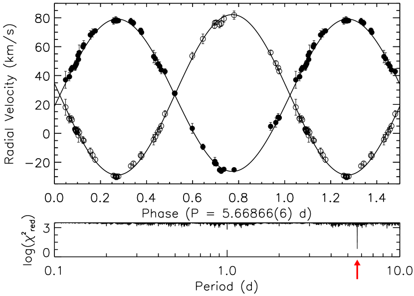
Figure 2: Top: The nearly sinusoidal fits to the radial velocities of the two A stars phased by a period of $5.66866\,\text{d}$. Bottom: The reduced $\chi^{2}$ distribution yielded by the period fitting routine applied to one of the A stars. The $5.66866\,\text{d}$ period is indicated by the red arrow.

We chose a grid of periods ranging from $0.1$ to $10\,{\rm d}$ in increments of $10^{-5}\,{\rm d}$ ($\sim 1\,{\rm s}$). The amplitudes ($K_{1}=K_{2}$) and phase shifts ($\phi_{1}=|\phi_{2}-\pi|$) were defined by the maximum $v_{r}$ separation of $109\,{\rm km\,s}^{-1}$ (i.e. phase $0.994$ where this phase corresponds to the phase of the B star’s maximum longitudinal magnetic field derived in Section 5). The analysis then involves assigning radial velocities to each of the A star components based on a best-fitting period of $5.6687{\rm d}$. An alternative means of identifying the orbital period uses the fact that the quantity $|v_{r,1}-v_{r,2}|$ varies with a period of $2P_{\rm orb}$, as outlined by Hareter et al. (2008). Applying this method yields a similar value of $P_{\rm orb}=5.6680(6)\,{\rm d}$.

With the radial velocities of the two A stars correctly assigned to each individual component, a more precise analysis of the binary orbital parameters was carried out using orbitx, a fortran code later adapted to idl which determines the best-fitting $P_{\rm orb}$, time of periastron passage ($T$), eccentricity ($e$), longitude of the periastron ($\omega$), semi-amplitudes of each component’s radial velocities ($K_{1}$ and $K_{2}$), and the radial velocity of the center of mass ($\gamma$) (Tokovinin, 1992). This calculation yielded $P_{\rm orb}=5.66866(6)\,{\rm d}$, $T=2456658.172\pm 1.652$, $e=0.003_{-0.003}^{+0.006}$, $\omega=82\pm 105\degree$, $K_{1}=55.5\pm 0.4\,{\rm km\,s^{-1}}$, $K_{2}=52.7\pm 0.4\,{\rm km\,s^{-1}}$, and $\gamma=26.5\pm 0.2\,{\rm km\,s^{-1}}$. These results imply a mass ratio of $M_{1}/M_{2}=1.05\pm 0.02$, a projected total mass of $(M_{1}+M_{2})\sin^{3}{i}=0.186\pm 0.008$, and a projected semi-major axis of $a\sin{i}=0.0564\pm 0.0008$. These values are listed in Table 4. Fig. 2 shows the radial velocities of the A stars phased by the $5.66866\,{\rm d}$ orbital period and compared with the radial velocities computed from the orbital solution.

Comparing $\langle v_{r,A}\rangle=25\pm 3\,{\rm km\,s}^{-1}$ with the average B star $v_{r}$ of $20.5\pm 1.6\,{\rm km\,s}^{-1}$ and noting that no significant variability in $\langle v_{r,A}\rangle$ was detected over the $22$ year observing period implies a very long orbital period of the A binary about the B star. A lower limit for this period is derived in Section 3.2.

Table 4: Orbital parameters of the A+A binary.

$P_{\rm orb}\,({\rm d})$	$5.66866(6)$
$T$	$2456658.172\pm 1.652$
$e$	$0.003^{+0.006}_{-0.003}$
$\omega\,(\degree)$	$82\pm 105$
$K_{1}\,{\rm(km/s)}$	$55.5\pm 0.4$
$K_{2}\,{\rm(km/s)}$	$52.7\pm 0.4$
$\gamma\,{\rm(km/s)}$	$26.5\pm 0.2$
$M_{1}/M_{2}$	$1.05\pm 0.02$
$(M_{1}+M_{2})\sin^{3}{i}\,(M_{\odot})$	$0.186\pm 0.008$
$a\sin{i}\,{\rm(AU)}$	$0.0564\pm 0.0008$

3.2 SED fitting

Photometric fluxes of HD 35502 have been measured throughout the UV, visible, and near infrared spectral regions thereby allowing the temperatures and radii of the three stellar components to be constrained. Ultraviolet measurements were previously obtained at four wavelengths – $1565\,\rm{\AA}$, $1965\,\rm{\AA}$, $2365\,\rm{\AA}$, and $2749\,\rm{\AA}$ – by the $S2/68$ instrument on board the $TD1$ satellite (Thompson et al., 1978). Photometry spanning the visible spectrum were taken from the Geneva Observatory’s catalogue of $U$, $B$, $V$, $B_{1}$, $B_{2}$, $V_{1}$, and $G$ filters (Rufener, 1981). Additionally, infrared observations obtained by 2MASS ($J$, $H$, and $Ks$ filters) (Skrutskie et al., 2006) and WISE ($W1$ and $W2$ filters) (Wright et al., 2010) were used. The reported Geneva, 2MASS, and WISE magnitudes were converted to the flux units of ${\rm ergs\,s^{-1}\,cm^{-2}\,{\AA}^{-1}}$ using the zero points reported by Rufener & Nicolet (1988), Cohen, Wheaton & Megeath (2003), and Wright et al. (2010).

The reported photometric measurements of HD 35502 include the contributions from each of the three stellar components. This renders an SED fitting analysis particularly susceptible to degenerate solutions; however, speckle interferometry measurements obtained by Balega et al. (2012) provide additional photometric constraints on the system. They detected magnitude differences of $1.45\pm 0.02\,{\rm mag}$ and $1.21\pm 0.02\,{\rm mag}$ using filters centered on $5500\,\rm{\AA}$ and $8000\,\rm{\AA}$, respectively. The sources were reported to have angular separations of $69\pm 1\,{\rm mas}$ and $68\pm 1\,{\rm mas}$ in the two filters. The speckle companion is also identifed in observations obtained by Horch et al. (2001) with a consistent angular separation of $\rho<59\,{\rm mas}$.

In conjunction with the distance to HD 35502, the angular separations may be used to determine the associated linear separation. A distance of $d=430\pm 120\,\rm{pc}$ was inferred from the $2.35\pm 0.68\,\rm{mas}$ Hipparcos parallax (van Leeuwen, 2007). However, assuming HD 35502 to be a member of the Orion OB1a subassociation, we inferred a moderately more precise value of $400\pm 80\,{\rm pc}$ based on the subassociation’s reported average distance modulus of $\langle{\rm dm}\rangle=8.00\pm 0.46\,{\rm mag}$ (Brown, de Geus & de Zeeuw, 1994). The projected linear separation between the two speckle sources was then found to be $27\pm 5\,\rm{AU}$. The minimum orbital period of the A star binary system around the B star can then be approximated by assuming upper limit masses of $8\,M_{\odot}$ and $3\,M_{\odot}$ for the B and A stars, respectively (the actual masses are derived in Section 8). This implies an orbital period of $P_{\rm orb}\gtrsim 40\,\rm{yrs}$, which is consistent with the fact that no significant variations were detected in either the B star radial velocities or the A star binary’s systemic radial velocity.

Figure 3: Marginalized posterior probability distributions returned by the MCMC algorithm that was applied to the SED fitting. Each frame demonstrates the correlations that are apparent between various parameters, while the vertical and horizontal blue lines indicate the value of each parameter associated with the maximum likelihood solution (i.e. $T_{B}$, $T_{A}$, $R_{B}$, and $R_{A}$). The contours approximately correspond to $1-3\sigma$ confidence regions in increments of $0.5\sigma$; $\sigma_{T_{B}}$, $\sigma_{T_{A}}$, $\sigma_{R_{B}}$, and $\sigma_{R_{A}}$ indicate the value of each parameter’s $1\sigma$ region.

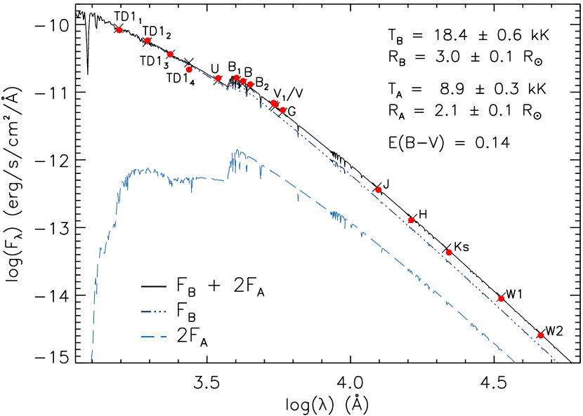
Figure 4: Comparisons between the observed photometry (red points) and the model SED (solid black curve). The dashed blue and dot-dashed black curves correspond to the model SEDs of the composite A star components (i.e. $2F_{A}(\lambda)$) and the B star, respectively. The black crosses indicate the flux obtained by multiplying the model SED by the transmission function of the associated filter.

The observed photometry was fit using atlas9 synthetic spectral energy distributions (SEDs) generated from the atmospheric models of Castelli & Kurucz (2004). The grid consists of models with effective temperatures ranging from $3.5-50.0\,\rm{K}$ and surface gravities spanning $\log{g}=0.5-5.0\,\rm{(cgs)}$, as described in detail by Howarth (2011). This grid was linearly interpolated in order to produce models with a uniform temperature and surface gravity resolution of $125\,\rm{K}$ and $0.01\,\rm{dex}$ for $T_{\rm eff}=5-25\,\rm{kK}$ and $\log{g}=3.0-4.75\,\rm{(cgs)}$. All of the SEDs were then multiplied by the transmission functions associated with each of the narrow band filters: TD1 $UV$ (Carnochan, 1982), Geneva (Rufener & Nicolet, 1988), 2MASS (Cohen, Wheaton & Megeath, 2003), and WISE (Wright et al., 2010).

Modelling the photometry of un-resolved multi-star systems using synthetic SEDs requires a large number of fitting parameters and therefore the solution is expected to be highly degenerate. The contribution to the total flux from each of the three stellar components depends on, among other factors, their effective temperatures, surface gravities, and radii. In order to reduce the number of solutions, we adopted a solar metallicity and a microturbulence velocity of $v_{\rm mic}=0\,{\rm km\,s}^{-1}$. As with many Bp stars, HD 35502’s primary exhibits chemical spots on its surface (see Section 6); however, on average, a solar metallicity may be adopted.

The high-resolution spectra of HD 35502 obtained by Narval, ESPaDOnS, and FEROS suggest that the two cooler A star components are approximately identical in terms of their $T_{\rm eff}$, $\log{g}$, and line-broadening parameters (see Section 3.3). If we assume that the two A stars contribute identically to the SED, the number of independent models required in the fitting routine is reduced from three to two thereby resulting in a total of six free parameters: $T_{\rm eff}$, $\log{g}$, and the stellar radius, $R$, for both the B star and the (identical) A stars.

The effective temperature of a star inferred from fitting model SEDs to photometry is highly dependent on the assumed colour excess, $E(B-V)$. Given HD 35502’s probable location within the Orion OB1a association (Landstreet et al., 2007), the extinction caused by gas and dust is expected to be significant. Indeed, Sharpless (1952) and Lee (1968) report values (without uncertainties) of $E(B-V)$ of $0.13$ and $0.14$, respectively. We used the method of Cardelli, Clayton & Mathis (1989) with an adopted to selective total extinction ratio of $R(V)=3.1$ in order to deredden the observed photometry. Small differences in the resulting best-fitting parameters of $<3$ per cent were found by using an $E(B-V)$ of $0.13$ or $0.14$. Although we investigated how our analysis was affected by varying the colour excess from $0.0-0.2$, the final effective temperatures are reported after assuming $E(B-V)=0.14$.

We found that a Markov Chain Monte Carlo (MCMC) fitting routine provided a suitable means of determing the most probable solution while simultaneously revealing any significant degeneracies. This was carried out by evaluating the likelihood function yielded by a set of randomly selected fitting parameters drawn from a prior probability (see e.g. Wall & Jenkins, 2003). For each iteration, the derived likelihood is compared with that produced by the previous iteration. If a new solution is found to yield a higher quality of fit (higher likelihood), these parameters are adopted, otherwise, the previous solution is maintained. In order to broadly sample the solution space, the MCMC algorithm is designed to adopt poorer fitting solutions at random intervals thereby preventing a local (but not global) maximum likelihood from being returned.

Uniform prior probability distributions (flat priors) were defined for $T_{\rm eff}$, $\log{g}$, and $R$, where the latter was constrained within $1.0-10.0\,R_{\odot}$. The two speckle observations (Balega et al., 2012) were then included in the total prior probability as monochromatic flux ratios (i.e. magnitude differences) at $5500\,{\rm\AA}$ and $8000\,{\rm\AA}$. We assumed that the reported $0.02\,{\rm mag}$ uncertainties correspond to $1\sigma$ significance. The marginalized posterior probability distributions produced after $10^{6}$ iterations in the Markov Chain are shown in Fig. 3.

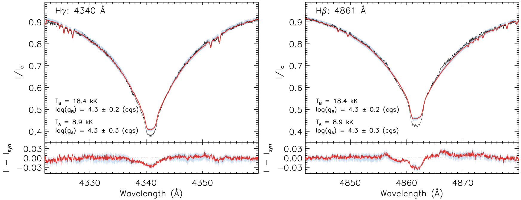
Figure 5: Top: Comparisons between the best-fitting synthetic (red) and observed (black) H lines, H$\gamma$ (left) and H$\beta$ (right). The filled blue region indicates the total uncertainty associated with $\log{g_{B}}$ and $\log{g_{A}}$. The observations occur at phase $0.49$ in the B star’s rotational period (see Section 4) when the weakest emission is visible in the wings of H$\beta$. Bottom: The residuals associated with the model spectrum (red).

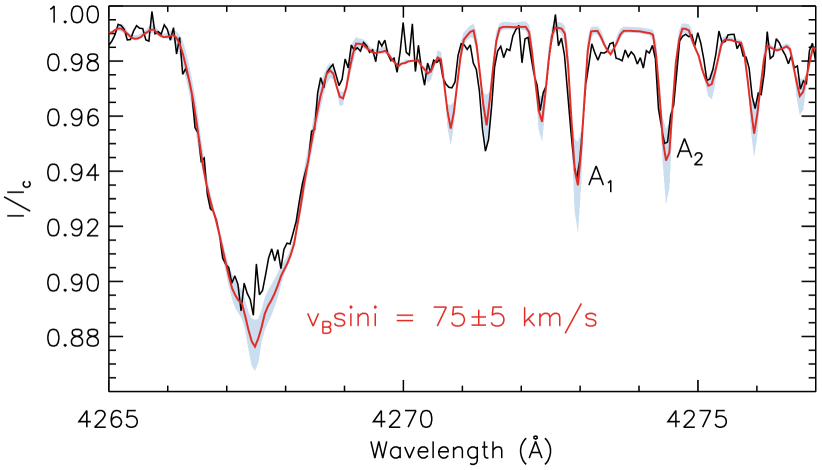
Figure 6: A subsample of the wavelength region used to determine the luminosity ratio, $L_{B}/L_{A}$. The red curve corresponds to the best-fitting model spectrum; the filled blue region indicates the total uncertainty associated with a $v_{B}\sin{i}$ of $\pm 5\,{\rm km\,s}^{-1}$ as determined by fitting various metal lines. The black curve shows the observed spectrum. The Fe i$\,\lambda 4273$ lines of the two A star components are labeled as ‘A₁’ and ‘A₂’.

The most probable effective temperatures for the B and A star models were found to be $18.4\pm 1.2\,{\rm kK}$ and $8.9\pm 0.6\,{\rm kK}$, respectively, where the uncertainties correspond to the $93^{\rm rd}$ percentile (approximately $2\sigma$). The fitting parameters used to derive the stellar radii, $R_{B}$ and $R_{A}$, depend on the distance to HD 35502 (i.e. as a scaling factor given by $R_{\ast}^{2}/d^{2}$). Although the posterior probability distributions for $R_{B}$ and $R_{A}$ both yield $2\sigma$ uncertainties of $0.2\,R_{\odot}$, the consideration of the relatively large distance uncertainty ($d=400\pm 80\,{\rm pc}$) implies larger uncertainties of $\delta R_{B}=0.6\,R_{\odot}$ and $\delta R_{A}=0.4\,R_{\odot}$. The most probable radii and their uncertainties found from the MCMC analysis are then given by $R_{B}=3.0\pm 0.6\,R_{\odot}$ and $R_{A}=2.1\pm 0.4\,R_{\odot}$. The derived temperatures and stellar radii are listed in Table 5. The analysis was insensitive to changes in $\log{g}$ as indicated by an essentially flat posterior probability distribution; therefore, no definitive surface gravity can be reported. Comparisons between the observed photometry and the best-fitting model are shown in Fig. 4, where we have adopted $\log{g}=4.3$ for both the A and B models as derived in Section 3.3.

The model B star flux ($F_{B}$) and the model binary A star flux ($2F_{A}$) can be used to verify our initial assumption that the two components detected in the speckle observations do indeed correspond to the central B star and the A star binary system. The models can be compared with the speckle observations by calculating the flux ratios, $2F_{A}(\lambda)/F_{B}(\lambda)$, at the speckle observation wavelengths. Both $F_{A}(\lambda)$ and $F_{B}(\lambda)$ are integrated over wavelength intervals of $200\,{\rm\AA}$ and $1000\,{\rm\AA}$ (i.e. the FWHM of the filters used by Balega et al., 2012) centered at $5500\,{\rm\AA}$ and $8000\,{\rm\AA}$, respectively. We then obtain magnitude differences of $\Delta m_{\rm syn}(5500\,{\rm\AA})=1.46$ and $\Delta m_{\rm syn}(8000\,{\rm\AA})=1.23$. These values yield a negligible discrepancy with the speckle observations of $1$ per cent at $\lambda=5500\,{\rm\AA}$ and $2$ per cent at $\lambda=8000\,{\rm\AA}$.

Table 5: Stellar parameters of HD 35502.

Sp. Type1	B5IVsnp+A+A
${\rm\pi}$ (mas)2	$2.35\pm 0.68$
$\langle{\rm dm}\rangle$ (mag)3	$8.00\pm 0.46$
$d$ (pc)	$400\pm 80$
Photometry
$V$ (mag)4	$7.331\pm 0.004$
$E(B-V)$ (mag)5	$0.14$
B Star Parameters
$T_{\rm eff}\,(\text{kK})$	$18.4\pm 0.6$
$\log(g)\,(cgs)$	$4.3\pm 0.2$
$v\sin{i}\,({\rm km\,s}^{-1})$	$75\pm 5$
$\log{L/L_{\odot}}$	$3.0\pm 0.3$
$M/M_{\odot}$	$5.7\pm 0.6$
$R_{p}/R_{\odot}$	$3.0^{+1.1}_{-0.5}$
$R_{\rm eq}/R_{\odot}$	$3.1^{+1.8}_{-0.4}$
$\tau_{\rm age}\,(\text{Myr})$	$20\pm 20$
$P_{\rm rot}\,(\text{d})$	$0.853807(3)$
A Star Parameters
$T_{\rm eff}\,(\text{kK})$	$8.9\pm 0.3$
$\log(g)\,(cgs)$	$4.3\pm 0.3$
$v\sin{i}\,({\rm km\,s}^{-1})$	$12\pm 2$
$\log{L/L_{\odot}}$	$1.4\pm 0.3$
$M/M_{\odot}$	$2.1\pm 0.2$
$R/R_{\odot}$	$2.1\pm 0.4$
$\tau_{\rm age}\,(\text{Myr})$	$<630$

• Table references: ¹Abt & Levato (1977), ²van Leeuwen (2007), ³Brown, de Geus & de Zeeuw (1994), ⁴Rufener (1981), ⁵Lee (1968).

3.3 Spectral line fitting

Several properties of HD 35502’s three stellar components may be estimated through comparisons with synthetic spectra (e.g. the surface gravity, line broadening characteristics, etc.). We carried this out using local thermodynamic equilibrium (LTE) models generated with synth3 (Kochukhov, 2007). The code computes disc-integrated spectra using spectral line data provided by VALD (Kupka et al., 2000) obtained using an extract stellar request for a specified effective temperature, surface gravity, and microturbulence velocity in conjunction with atlas9 atmospheric models (Kurucz, 1993). The synthetic spectra can then be convolved with the appropriate functions in order to account for instrumental and rotational broadening effects.

The ESPaDOnS, Narval, and FEROS observations were normalized using a series of polynomial fits to the continuum. The relatively shallow ($\approx 5$ per cent of the continuum) and narrow lines produced by the two A stars made the spectral line modelling inherently uncertain. For instance, the typical root mean square of the continuum near the A stars’ Mg i$\,\lambda 4703$ lines was found to be approximately $14$ per cent of the line depth. Thus, the SNRs of the majority of the A star lines were relatively low. This was mitigated to some extent by binning the observed spectra with a bin width of $\approx 0.03\,{\rm\AA}$ (i.e. $2$ pixels). In order to account for the instrumental profile of the ESPaDOnS and Narval observations, the synthetic spectra were convolved with a Gaussian function assuming a resolving power of $R=65\,000$; similarly, the FEROS spectra were fit after convolving the synthetic spectra assuming $R=48\,000$.

The quality of fit yielded by the total normalized synthetic spectrum ($F_{\rm tot}$) depends not only on $T_{\rm eff}$ of the three models but also on their (relative) luminosities: ${F_{\rm tot}=(\sum_{i}L_{i}F_{i})/\sum_{i}L_{i}}$, where $L_{i}$ and $F_{i}$ are the luminosities and synthetic spectra of the $i^{\rm th}$ component. We adopted the $18.4\,{\rm kK}$ and $8.9\,{\rm kK}$ values associated with the B and two A stars obtained from the SED fitting (Section 3.2). Moreover, we assumed that the luminosities of the two A stars are equal, thereby reducing the number of degrees of freedom in the spectral line fitting analysis.

With $T_{\rm eff}$ specified, the stellar luminosities can be estimated through various methods. We found that the best results were obtained by letting the luminosity ratio of the B and A star models, $L_{B}/L_{A}$, be a free parameter and subsequently finding the minimum $\chi^{2}$ fit for a given surface gravity ($\log{g}$) and rotational broadening ($v\sin{i}$). This was carried out using the observed spectra for which the two A stars were most widely separated in wavelength (phase $0.994$ in Fig. 2) in the wavelength range of $4200-4300\,{\rm\AA}$. This region was chosen because of the presence of the strong and essentially non-variable C ii line produced by the B star along with many A star lines of various elements (e.g. Fe, Ti, Cr, Mn). Most importantly, this wavelength range is free of B star lines exhibiting obvious chemical abundance anomalies and variability such as those observed from He. A subsample of this region containing C ii$\,\lambda 4267$ is shown in Fig. 6. This technique yielded $L_{B}/L_{A}=5.2$, which is consistent with the median value implied by the SED fitting analysis – within $4000\,{\rm\AA}\leq\lambda\leq 6000\,{\rm\AA}$ – of $8.4^{+4.1}_{-2.4}$. Ultimately, using an $L_{B}/L_{A}$ of $5.2$ instead of $8.4$ produced a moderate increase of $1.1\sigma$ in the best-fitting solution’s overall quality of fit.

$\log{g}$ and $v\sin{i}$ of HD 35502’s three components were then fit using various B and A star lines while recalculating the best-fitting $L_{B}/L_{A}$ for every change in the parameters. As a result of the presumed chemical peculiarities and line variability of the B star (see Section 6) and the limited number of lines, $\log{g_{B}}$ could not be reliably constrained using He or metal lines (e.g. Mg i and Mg ii). Instead, we relied upon the wings of the strong and broad Balmer lines. In particular, the observations of H$\beta$, H$\gamma$, and H$\delta$ obtained at a phase of $0.49$ in the B star’s rotational period (the phase of minimum emission) were used in order to minimize the effects of emission. Several metal lines were used to constrain $v_{B}\sin{i}$ such as C ii$\,\lambda 4267$, S ii$\,\lambda 5640$, and Fe ii$\,\lambda 5780$. $\log{g_{B}}$ and $v_{B}\sin{i}$ were found to be $4.3\pm 0.2\,{\rm(cgs)}$ and $75\pm 5\,{\rm km\,s}^{-1}$, respectively. Examples of the best-fitting model spectra are shown in Fig. 5; the adopted range in $v_{B}\sin{i}$ is shown in Fig. 6.

The surface gravity and rotational broadening of the two A stars were fit simultaneously using several Fe ii and Mg i lines. Their best-fitting $\log{g}$ and $v\sin{i}$ values were found to be $4.3\pm 0.3\,{\rm(cgs)}$ and $12\pm 2\,{\rm km\,s}^{-1}$, respectively. Two examples of the modelled A star lines are shown in Fig. 7.

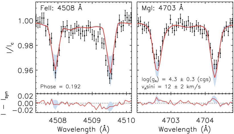
Figure 7: Comparisons between best-fitting model (red) and observed (black points) Fe ii (left) and Mg i (right) lines used to constrain the surface gravity and rotational broadening of the two A stars; the filled blue region indicates the total uncertainties associated with $v_{A}\sin{i}$ and $\log{g_{A}}$. The phase corresponds to the maximum observed separation between the two binary components.

3.4 Hertzsprung-Russell Diagram

The masses, ages, and polar radii of HD 35502’s three stellar components may be estimated by comparing their positions on the Hertzsprung-Russell diagram (HRD) with theoretical isochrones.

In order to determine the B star’s luminosity, we used the $18.4\pm 0.6\,{\rm kK}$ effective temperature and $3.0\pm 0.6\,R_{\odot}$ radius derived from the three star SED fit discussed in Section 3.2. The Stefan-Boltzmann law then yields a luminosity of $\log{L/L_{\odot}}=3.0^{+0.4}_{-0.5}$. Similarly, the position of the A stars on the HRD can be identified using $T_{\rm eff}=8.9\pm 0.3\,{\rm kK}$ and $R_{A}=2.1\pm 0.4\,R_{\odot}$. We calculate an A star luminosity of $\log{L/L_{\odot}}=1.4\pm 0.3$. The HRD positions of the B and A stars are shown in Fig. 8.

The masses ($M$) and polar radii ($R_{p}$) associated with a given $T_{\rm eff}$ and $\log{L/L_{\odot}}$ were determined using a grid of Geneva model isochrones generated by Ekström et al. (2012). The grid is calculated for the evolutionary timescale beginning with the zero-age main sequence up until the core carbon-burning phase for masses of $0.8-120\,M_{\odot}$. The microturbulence velocity was fixed at $v_{\rm mic}=0.0\,{\rm km\,s}^{-1}$ and a solar metallicity of $Z=0.014$ was assumed. In the case of HD 35502’s central B star, the ratio of the angular velocity to the critical angular velocity, $\Omega/\Omega_{c}$, is known to be significant based on the $0.853807(3)\,{\rm d}$ rotational period (see Section 4). Its position on the HRD was therefore compared against several additional grids calculated using $\Omega/\Omega_{c}=0.4-0.9$ in increments of $0.1$ (Georgy et al., 2013). While no significant difference in the inferred $M$ was apparent (i.e. $<4$ per cent), $R_{\rm p}$ was found to decrease by as much as $15$ per cent.

In order to select the most accurate grid of isochrones and thus, the most accurate $R_{\rm p}$, $\Omega/\Omega_{c}$ must first be estimated. Since $\Omega_{c}$ depends on both the mass and polar radius, it was calculated using the parameters derived from each grid of isochrones. Using $P_{\rm rot}$ inferred in Section 4 to determine $\Omega$, a range of $\Omega/\Omega_{c}$ values were found. The appropriate grid was then chosen based on whichever $\Omega/\Omega_{c}$ most closely agreed with the $\Omega/\Omega_{c}$ associated with the isochrone grid. A calculated $\Omega/\Omega_{c}$ of $0.53$ yielded the best agreement; we found $R_{{\rm p},B}=3.0^{+1.1}_{-0.5}\,R_{\odot}$ and $M_{B}=5.7\pm 0.6\,M_{\odot}$ using the $\Omega/\Omega_{c}=0.5$ isochrones. These results imply an equatorial radius of $R_{{\rm eq},B}=3.2^{+1.6}_{-0.6}\,R_{\odot}$. Using von Zeipel’s law (von Zeipel, 1924), we estimate that the ratio of $T_{\rm eff}$ between the pole and the equator is approximately $1.02$.

The two A stars’ $M$ and $R_{\rm p}$ were inferred using the $\Omega/\Omega_{c}=0.0$ isochrone grid. The $T_{\rm eff}$ and $\log{L/L_{\odot}}$ derived from the three star SED fit then yielded $R_{{\rm p},A}=2.0^{+0.8}_{-0.5}\,R_{\odot}$ and $M_{A}=2.1\pm 0.2\,M_{\odot}$. We note that both $R_{{\rm p},B}$ and $R_{{\rm p},A}$ are consistent with $R_{B}$ and $R_{A}$ derived in Section 3.2.

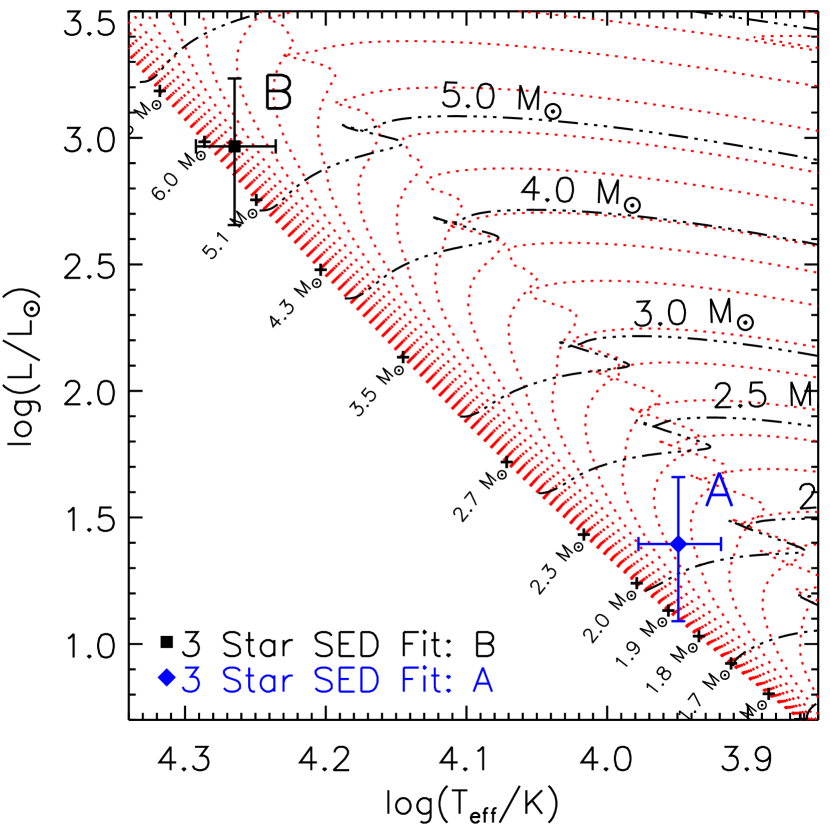
Figure 8: The positions of HD 35502’s A and B star components are indicated by the blue diamond and black square. The evolutionary tracks (black dot-dashed lines) and isochrones (red dotted lines) assume a non-rotating star of solar metallicity (Ekström et al., 2012).

Figure 9: H, He+metal, He, C, Si, and Fe Stokes $I$ and $V$ LSD profiles generated from a $T_{\rm eff}=26\,{\rm kK}$, $\log{g}=4.0\,{\rm(cgs)}$ line mask. The profiles are all phased by the B star’s rotational period of $0.853807\,{\rm d}$.

4 Rotational period

Several observed properties of HD 35502 exhibit periodic variability with varying significance. In order to correctly interpret the origin of these variations, it is crucial to identify the periods, the phases at which the maxima and minima occur, and amplitudes with which they occur. This was carried out using the same procedure discussed in Section 3.1 in which the orbital solution of the A star binary was derived.

We first assumed a sinusoidal fit to the data, $f(t)$, given by $f(t)=C_{0}+C_{1}\sin{(2\pi[t-t_{0}]/P+C_{2})}$, where $P$ is the period of variability, $t$ is the observation’s HJD, $t_{0}$ is the HJD corresponding to phase $0$, and $C_{0}$, $C_{1}$, and $C_{2}$ are fitting parameters. A $\chi^{2}$ distribution was then generated using periods ranging from $0.1$ to $10.0\,{\rm d}$ in increments $\sim 1\,{\rm s}$. The best-fitting period was inferred from the minimal $\chi^{2}$ solution and the $3\sigma$ $\chi^{2}$ interval was taken as the associated uncertainty. The uncertainties in the three fitting parameters were estimated using a $1\,000$ iteration bootstrapping analysis. The statistical significance of each derived period was evaluated by comparing the quality of the sinusoidal fit to that yielded by a constant fitting function given by $f(t)=C_{0}$, where $C_{0}$ is a time-independent fitting parameter. The difference between the minimal $\chi^{2}$ values associated with the constant fit ($\chi^{2}_{\rm const}$) and sinusoidal fit ($\chi^{2}_{\rm sin}$) were then calculated. Any sinusoidal fit having $\chi^{2}_{\rm const}-\chi^{2}_{\rm sin}\geq 3\sigma$ was considered to be statistically significant.

Various periods were found when this procedure was applied to the longitudinal field measurements ($\langle B_{z}\rangle$, see Section 5) along with the multiple photometry and equivalent width (EW) measurements (see Section 6). The analyses of nearly all datasets yielded statistically significant variability, with over half corresponding to a unique period near $0.85\,{\rm d}$. They were found to be equal to one another within $\approx 10\,{\rm sec}$ with typical uncertainties $\lesssim 10\,{\rm s}$ and were therefore averaged to obtain a period of $0.85382(7)\,{\rm d}$. However, when the H$\alpha$ EWs were phased with this period, the oldest measurements showed an $\approx 0.1$ phase offset relative to the more recent measurements. This discrepancy was resolved by adopting the best-fitting ephemeris derived from the H$\alpha$ EWs of

$$JD=2456295.812850\pm 0.853807(3)\cdot E$$ (2)

where the reference JD ($2456295.812850(3)$) corresponds to the epoch of $\langle B_{z}\rangle$ maximum magnitude. Therefore, while the general accuracy of the rotational period is established by the diverse photometric, spectroscopic, and magnetic data sets, the adopted value and its precision correspond to those implied by the H$\alpha$ EWs.

The periodic variability of $\langle B_{z}\rangle$ can be explained, in part, as a consequence of a stable oblique magnetic field configuration that is modulated by the star’s rotation. Similarly, rotationally-modulated variations exhibited by the equivalent widths of various spectral lines can be produced by at least two mechanisms: (1) non-uniform distributions of chemicals on the stellar surface and (2) hot plasma accumulating in the star’s magnetosphere resulting in emission and absorption. All of these phenomena are commonly exhibited by magnetic B-type stars (e.g. Landstreet & Borra, 1978; Leone et al., 2010; Bohlender & Monin, 2011). Therefore, we conclude that the ephemeris given by Eqn. 2 is the B star’s rotational period.

5 Magnetic field

Zeeman signatures produced by a magnetic star in the HD 35502 system were detected in circularly polarized (Stokes $V$) ESPaDOnS and Narval observations. They were found to be coincident with the B star’s spectral lines regardless of the inferred velocities of the two A stars. We therefore assumed the detected field to be entirely produced by the B star.

The Stokes $V$ Zeeman signature associated with H$\beta$ yielded 18 definite detections (DDs), 1 marginal detection (MD), and 7 non-detections (NDs) based on the detection criterion outlined by Donati et al. (1997). The SNRs of the observed signatures were optimized using the LSD procedure (Donati et al., 1997; Kochukhov, Makaganiuk & Piskunov, 2010) introduced in Section 3.1. A master line mask containing He and metal lines was generated using data obtained from VALD (Kupka et al., 2000) with a specified $T_{\rm eff}$, $\log{g}$, and microturbulence velocity ($v_{\rm mic}$). All Balmer lines were also removed along with any regions affected by atmospheric absorption (i.e. telluric lines). Several single element line masks were subsequently generated from the He+metal mask by retaining only specific chemical elements including He, C, Si, Fe, and Mg. Clearly, the magnitudes of $\langle B_{z}\rangle$ derived using different elements will be affected by any non-uniform distribution of chemicals across the star’s surface. Therefore, our analysis also includes measurements obtained using H lines (both from LSD profiles and H$\beta$) which do not typically exhibit non-solar abundances or non-homogeneous surface distributions (i.e. chemical spots). A H line mask was generated in which the H lines exhibiting moderate emission (e.g. H$\beta$ and H$\alpha$) were removed. The resultant mask contained three H i lines: H i$\,\lambda 3970$, H i$\,\lambda 4102$, and H i$\,\lambda 4340$.

Two approaches were used to isolate the B star lines from the A star lines using LSD. The first method used a mask generated with $T_{\rm eff}=15\,{\rm kK}$, $\log{g}=4.0\,{\rm(cgs)}$, and $v_{\rm mic}=0\,{\rm km\,s^{-1}}$ which yielded LSD profiles with clear Stokes $I$ contributions from all three stellar components. The narrow line components associated with the two A stars were then fit by Gaussian functions which were subsequently subtracted from the Stokes $I$ profiles. We found that this method could not be consistently applied to all observations. Moreover, the quality of the Gaussian fits was dramatically reduced when applied to the C, Si, and Fe line masks.

The second method used the same $\log{g}$ and $v_{\rm mic}$ with a significantly higher temperature of $T_{\rm eff}=26\,{\rm kK}$. This yielded LSD profiles with minimal contributions from the two A stars. The Stokes $I$ and $V$ LSD profiles generated using the $T_{\rm eff}=26\,{\rm kK}$ line mask for H, He+metal, He, C, Si, and Fe are shown in Fig. 9, phased according to Eqn. 2. Aside from the Si and Fe LSD profiles, no strong contributions from the A star Stokes $I$ profiles can be discerned.

Each ESPaDOnS and Narval spectropolarimetric observation includes a diagnostic null which may be used to evaluate the significance of any polarized signal. No spurious signals were detected in any of the diagnostic null profiles.

Figure 10: H$\beta$ longitudinal magnetic field measurements phased by the rotational period (Eqn. 2). The measurements obtained from Narval (open circles), ESPaDOnS (filled circles), and dimaPol (filled triangles) are shown along with the best fitting sinusoid (solid black).

$\langle B_{z}\rangle$ was inferred from each of the Stokes $I$ and $V$ LSD profiles, as well as from H$\beta$, using equation (1) of Wade et al. (2000). We used a wavelength of $500\,{\rm nm}$ with a Landé factor of $1.2$ for the He and metal mask measurements and a Landé factor of unity for the H mask and H$\beta$ measurements. The Doppler shift produced by the B star’s radial velocity of $\approx 20\,{\rm km\,s}^{-1}$ was subtracted from each LSD profile. The Stokes $I$ and $V$ profiles were then normalized to the continuum intensity at a velocity of $v=-125\,{\rm km\,s}^{-1}$, where the average Stokes $V$ intensity is approximately zero. An integration range of $v\in[-110,110]\,{\rm km\,s}^{-1}$ was then used in the calculation of $\langle B_{z}\rangle$ for each of the LSD profiles (i.e. H, He+metal, He, C, Si, and Fe); for the H LSD profiles and H$\beta$ line, this integration range corresponds to the width of the Doppler core. The values of $\langle B_{z}\rangle_{{\rm H}\beta}$ inferred from the Narval, ESPaDOnS, and dimaPol observations, along with the status of their detections, are listed in Tables 1 and 2. $\langle B_{z}\rangle$ derived from the H, He, and metal LSD profiles are listed in Table 7.

High resolution spectropolarimetry is essentially insensitive to the polarization in the wings of the Balmer lines. As an example of how the Doppler cores of Balmer lines may be used to infer $\langle B_{z}\rangle$, see Fig. 2 of (Landstreet et al., 2015), who explain the method in some detail. Our measurements obtained in the context of the current paper, as well as those obtained by (Sikora et al., 2015), demonstrate that this method results in longitudinal field intensity and variability in good agreement with other approaches.

Figure 11: Longitudinal magnetic field measurements phased by the rotational period (Eqn. 2). The measurements obtained from the H, He+metal, He, C, Si, and Fe line masks are shown along with their best fitting sinusoids (solid black). The fit to $\langle B_{z}\rangle_{\rm H}$ is shown as dashed black curves in the other panels.

All of the $\langle B_{z}\rangle$ measurements were found to exhibit statistically significant varitions with best-fitting periods ranging from $0.85380-0.85389\,{\rm d}$. Only the $\langle B_{z}\rangle$ values obtained using the Fe LSD profiles ($\langle B_{z}\rangle_{\rm Fe}$) yielded more than one period. Figures 10 and 11 show the $\langle B_{z}\rangle$ measurements inferred from H$\beta$ and the LSD profiles, respectively, phased by the B star’s rotational period (Eqn. 2). It is clear that the scatter of the $\langle B_{z}\rangle_{\rm He}$, $\langle B_{z}\rangle_{\rm Si}$, and $\langle B_{z}\rangle_{\rm Fe}$ measurements is significantly larger than that yielded by $\langle B_{z}\rangle_{\rm H}$, $\langle B_{z}\rangle_{\rm He+metal}$, and $\langle B_{z}\rangle_{\rm C}$. This is likely caused by the presence of He, Si, and Fe chemical spots which are commonly observed on the surfaces of Bp stars. As discussed in Section 6, we find strong evidence for He and Si spots.

The mean and amplitude of the phased $\langle B_{z}\rangle$ measurements are defined by the fitting parameters $B_{0}$ and $B_{1}$ associated with the sinusoidal fitting function $\langle B_{z}\rangle=B_{0}+B_{1}\sin{(2\pi\theta+\phi)}$, where $\theta$ is the phase calculated using Eqn. 2 and $\phi$ is the phase shift. The most precise $B_{0}$ and $B_{1}$ values – as indicated by the uncertainties estimated using a $1\,000$ iteration bootstrapping analysis – were derived using H$\beta$, and the H and He+metal LSD profiles. They were found to be consistent within $2\sigma$. The lowest uncertaintes were obtained from the $\langle B_{z}\rangle_{\rm H}$ measurements, which yielded a mean and amplitude of $B_{0}=-1.41\pm 0.11\,{\rm kG}$ and $B_{1}=1.64\pm 0.16\,{\rm kG}$ where the uncertainties correspond to $3\sigma$.

If we assume that the field is characterized by an important dipole component, the sinusoidal variations in $\langle B_{z}\rangle$ imply that the dipole’s axis of symmetry is inclined (i.e. has an obliquity angle $\beta$) with respect to the star’s rotational axis. This interpretation, first described by Stibbs (1950), is known as the Oblique Rotator Model (ORM). Under the assumptions of the ORM, $\beta$ can be calculated from equation (3) of Preston (1967) which depends on $r\equiv|\langle B_{z}\rangle|_{\rm min}/|\langle B_{z}\rangle|_{\rm max}$ and the inclination angle, $i$, of the star’s axis of rotation. The value of $i$ can be determined using $P_{\rm rot}$ given by Eqn. 2, $v\sin{i}=75\pm 5\,{\rm km\,s}^{-1}$ derived in Section 3.3, and $R_{\rm eq}=3.2^{+1.6}_{-0.6}\,R_{\odot}$ listed in Table 5. We obtained a value of $i=24^{+8}_{-9}\,\degree$. The value of $r$ was determined from $B_{0}$ and $B_{1}$. Using the values inferred from the $\langle B_{z}\rangle_{\rm H}$ measurements, we obtained $r=0.08^{+0.09}_{-0.07}$. Finally, the obliquity angle was found to be $\beta=63\pm 13\,\degree$ using Eqn. (3) of Preston (1967).

In addition to the obliquity, the strength of the magnetic field’s dipole component, $B_{p}$, can be calculated by inverting equation (1) of Preston (1967) and letting $t=0$ correspond to $\langle B_{z}\rangle_{\rm max}$. We used a linear limb darkening constant that was averaged over the values derived by van Hamme (1993) for the $U$, $B$, $V$, $R$, and $I$ bandpasses. These specific filters were selected because of the approximate correspondance with the ESPaDOnS and Narval wavelength range. A value of $u=0.265$ was obtained after interpolating the published table for an effective temperature and surface gravity of $18.4\,{\rm kK}$ and $4.3\,{\rm(cgs)}$. $i$, $\beta$, and $u$ then yield $B_{p}=14^{+9}_{-3}\,{\rm kG}$. Similar obliquity angles and dipolar field strengths are derived using H$\beta$ along with the He+metal, He, C, and Si LSD profiles. $\langle B_{z}\rangle_{\rm Fe}$ exhibits significantly weaker and more uncertain values of $\beta=33^{+36}_{-27}\,\degree$ and $B_{p}=8^{+6}_{-3}$.

6 Emission and variability

Hot magnetic B-type stars are commonly found to exhibit spectral line variability either as a result of chemical spots (e.g. Kochukhov et al., 2015; Yakunin et al., 2015) or from the presence of a hot plasma beyond the stellar surface (e.g. Landstreet & Borra, 1978). Furthermore, photometric variability correlated with both of these phenomena, as well as with strong, coherent magnetic fields has been previously reported (e.g. Shore et al., 1990; Oksala et al., 2010).

Along with the $uvby$ photometric measurements listed in Table HD 35502: a hierarchical triple system with a magnetic B5IVpe primary, we also analyzed Hipparcos Epoch Photometry for variability. The catalogue (Perryman et al., 1997) contains 98 observations of HD 35502 which were obtained over a period of $3.1\,{\rm yrs}$. Three of these measurements have multiple quality flags reported and were therefore removed from our analysis. The remaining measurements have an average of $7.331\,{\rm mag}$, a standard deviation of $0.011\,{\rm mag}$, and an average uncertainty of $0.009\,{\rm mag}$.

The period searching routine described in Section 4 was applied to both the $uvby$ and Hipparcos data sets. All of the $uvby$ measurements were found to exhibit statistically significant variability; however, only $u$(v-c) and $v$(v-c) yielded unique periods of $0.8537(3)\,{\rm d}$. The analysis of the Hipparcos magnitudes ($H_{p}$) resulted in a best-fitting period of $0.8630(2)\,{\rm d}$ along with five other statistically significant periods ranging from $0.46$ to $1.7\,{\rm d}$. Fig. 12 shows the sinusoidal fits to $u$(v-c), $v$(v-c), $b$(v-c), $y$(v-c), and $H_{p}$ obtained when phased by the B star’s $0.853807\,{\rm d}$ rotational period given by Eqn. 2.

The variability of the spectral lines associated with HD 35502’s central B star is most easily detected by calculating EWs. We carried this out for a number of lines for which no significant absorption produced by the two A stars was evident. This included He i, C ii, and Si iii lines. The EWs of the He and metal lines were calculated using integration ranges of $[-100,100]\,{\rm km\,s}^{-1}$ and were normalized to the continuum just outside these limits. The Balmer line EWs (H$\alpha$, H$\beta$, and H$\gamma$) were measured by normalizing to the flux at $|v|\gtrsim 700\,{\rm km\,s}^{-1}$ and integrating over a velocity range of $[-600,600]\,{\rm km\,s}^{-1}$. The uncertainties in the EW measurements were then estimated using a bootstrapping analysis with $1\,000$ iterations. All of the calculated EWs and uncertainties are listed in and Tables HD 35502: a hierarchical triple system with a magnetic B5IVpe primary and 9.

The contributions of the two A stars to the total measured Balmer line EWs were approximated by comparing the synthetic EWs associated with the synth3 models discussed in Section 3.3. We found that the total synthetic spectrum (including the B star and the two A stars) yielded EWs of $5.6\,{\rm\AA}$ averaged over H$\alpha$, H$\beta$, H$\gamma$, and H$\delta$. A similar calculation applied to the single B star model yielded average Balmer line EWs of $4.7\,{\rm\AA}$ suggesting that the presence of the two A stars increase the EW measurements by a factor of $\approx 1.2$.

Figure 12: Photometric observations obtained using various filters and phased by the B star’s rotational period of $0.853807\,{\rm d}$. The top four panels show the $u$(v-c), $v$(v-c), $b$(v-c), and $y$(v-c) magnitude differences between HD 35502 (‘v’) and the non-variable comparison star, HD 35575 (‘c’). The bottom panel shows the Hipparcos Epoch Photometry measurements. The horizontal dotted lines indicate the best constant fit to the data.

Statistically significant variations were detected from EW measurements of H$\alpha$, H$\beta$, H$\gamma$, He i$\,\lambda 4713$, and Si iii$\,\lambda 4553$. We note that telluric absorption lines were not removed or minimized in the calculation of these EWs. A range of best-fitting periods were derived; however, only the H$\alpha$ and He i$\,\lambda 4713$ EW measurements yielded unique periods of $0.853807(3)\,{\rm d}$ and $0.85377(3)\,{\rm d}$, respectively. The strongest variability was measured from H$\alpha$ for which an amplitude of $0.51\pm 0.03\,{\rm\AA}$ was derived. Similar variability – both in terms of the phase of maximum emission and the best-fitting period – was also detected in H$\beta$ although, at a much lower amplitude of $0.08\pm 0.01\,{\rm\AA}$. The phased H$\alpha$ and H$\beta$ EWs exhibit a maximum emission at a phase of $0.99\pm 0.04$ and $0.0\pm 0.3$, respectively, and are therefore in phase with the $\langle B_{z}\rangle$ measurements. The He i$\,\lambda 4713$ EWs are approximately in anti-phase with respect to the $\langle B_{z}\rangle$ variation with minimum absorption occuring at a phase of $0.5\pm 0.1$.

Along with EWs, dynamic spectra were also computed by comparing various spectral lines with their respective average normalized intensity ($\langle I/I_{c}\rangle$). Both the dynamic spectra and the EWs of C ii$\,\lambda 4267$, He i$\,\lambda 4713$, Si iii$\,\lambda 4553$, H$\beta$, and H$\gamma$ are shown in Fig. 13. It is evident that He i$\,\lambda 4713$, Si iii$\,\lambda 4553$, and to a lesser extent, C ii$\,\lambda 4267$, show absorption features crossing from negative to positive velocities. These features suggest the presence of chemical spots on the B star’s surface. The most obvious spot is associated with He i, which exhibits a maximum absorption at a phase of $0.0\pm 0.1$ and is therefore coincident with the epoch of maximum $\langle B_{z}\rangle$ magnitude. Assuming that the star’s magnetic field consists of a strong dipole component as discussed in Section 5, this result suggests that He is more concentrated near the field’s negative pole. Enhanced He abundances on the surfaces of magnetic Bp stars have been commonly reported to coincide with either the magnetic equator or magnetic poles (e.g. Neiner et al., 2003; Bohlender & Monin, 2011; Grunhut et al., 2012; Rivinius et al., 2013).

A similar plot of the dynamic spectrum and EWs of H$\alpha$ is shown in Fig. 14, where the additional DAO and CFHT spectra are also included. In order to reduce normalization errors, all of the H$\alpha$ spectra were consistently normalized using a linear fit to the measured flux at velocities of $\pm 600\,{\rm km\,s}^{-1}$. The observed spectra are compared with the synthetic spectrum ($I_{\rm syn}$) discussed in Section 3.3 rather than the average observed spectrum. $I_{\rm syn}$ includes the contributions from the A stars which move (in velocity space) relative to the B star throughout the B star’s rotational period. Therefore, this method results in a greater contrast between the emission and absorption features associated only with the B star. Strong, nearly symmetrical emission peaks are observed at a distance of $\approx 4\,R_{\ast}$ at a phase of $0.0$. The intensity of this emission is observed to decrease by a factor of $\approx 2$ at a phase of $0.5$. Similarly, the ratio between the maximum core emission (at phase $0.25$) and minimum core emission (at phase $0.5$) is also found to be $\approx 2$.

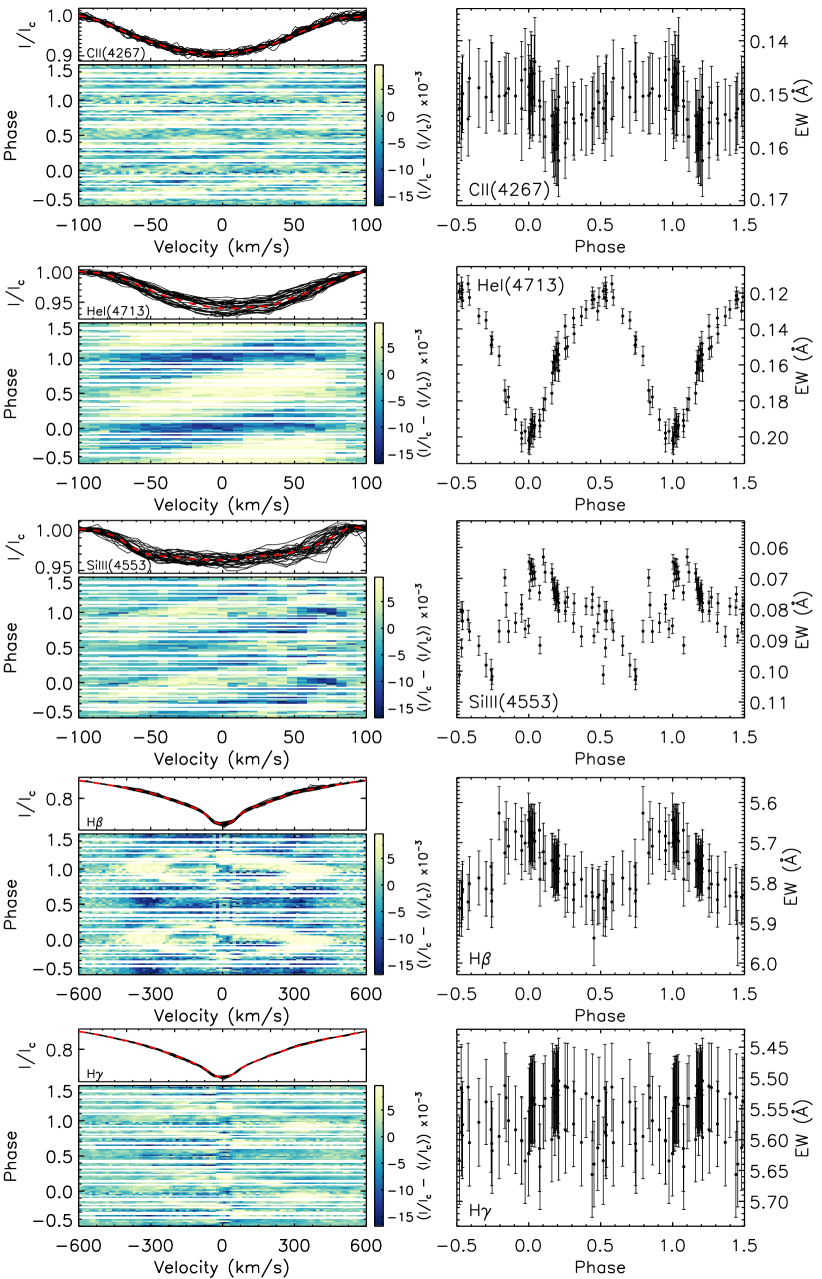
Figure 13: Left: Dynamic spectra of various H i, He i, C ii, and Si iii lines. A low-pass filter has been applied to the spectrum in order to minimize the A star contributions and tellurics. Each set of observations are compared with the average spectrum (dashed red). Right: Measured equivalent widths associated with the lines shown in the dynamic spectra plots. All of the measurements are phased by the B star’s rotational period of $0.853807\,{\rm d}$.

The standard interpretation of the broad H$\alpha$ emission peaks that are associated with a small number of magnetic B-type stars is that they are produced by two dense clouds of hot plasma, trapped in the magnetic field above the stellar surface, which co-rotate with the star (e.g. Walborn & Hesser, 1976; Landstreet & Borra, 1978). Under the assumption that the cloud is optically thin, one would expect the same blue shifted emission feature to be observed half a rotational cycle later shifted towards redder wavelengths (e.g. in Fig. 14, the blue emission peak occuring at phase 0.0 should reappear red shifted at phase 0.5). The fact that the strength of both the blue and red shifted emission peaks decrease between phase 0.0 and phase 0.5 suggests that the plasma clouds are, to an extent, optically thick. The relatively large decrease in emission is currently unprecedented amongst the known CM hosting stars; however, a more moderate decrease in HR 5907’s H$\alpha$ emission is shown in Fig. 15 of Grunhut et al. (2012).

Adopting the standard interpretation, the trajectories of the H$\alpha$-emitting clouds may be approximately inferred by fitting the velocities at which the peak emission is found on either side of the H$\alpha$ core as a function of rotational phase. The resulting fits suggest that the plasma clouds follow nearly circular trajectories as indicated by the two dashed curves shown in Fig. 14. The mechanism by which this plasma is confined is discussed in the following section.

7 Magnetosphere

As described by ud-Doula, Owocki & Townsend (2008), various characteristics of a star’s magnetosphere may be inferred by comparing two parameters: the Kepler radius, $R_{K}$, and the Alfvén radius, $R_{\rm Alf}$. $R_{K}$ is the radius at which the gravitational force is balanced by the centrifugal force in a reference frame that is co-rotating with the star. $R_{\rm Alf}$ characterizes the point within which the magnetic field dominates over the wind and approximately corresponds to the extent of the closed field loops (ud-Doula & Owocki, 2002; ud-Doula, Owocki & Townsend, 2008). Their ratio, $R_{\rm Alf}/R_{K}$, can therefore be used to define a magnetosphere as either dynamical ($R_{\rm Alf}/R_{K}<1$) or centrifugal ($R_{\rm Alf}/R_{K}>1$) (Petit et al., 2013). It also serves as an indicator of the volume of the magnetosphere: those stars having comparatively larger $R_{\rm Alf}/R_{K}$ will be capable of confining the emitted wind at larger radii. Furthermore, since a stronger field would be capable of confining more mass, a correlation between the Alfvén radius and the magnetosphere’s density may be expected.

Using the mass and rotational period of HD 35502’s B star, we find a Kepler radius of $R_{K}=2.1^{+0.4}_{-0.7}\,R_{\ast}$, where $R_{\ast}$ is the stellar radius at the magnetic equator. We approximate $R_{\ast}$ using $R_{\rm eq}$ since this corresponds to the stellar radius at the latitude where the plasma is expected to accumulate. The Alvén radius is estimated using equation (9) of ud-Doula, Owocki & Townsend (2008) for a dipole magnetic field. This expression requires the calculation of the wind confinement parameter, $\eta_{\ast}$, which in turn depends on the dipole magnetic field strength, the equatorial radius, the terminal wind speed ($V_{\infty}$), and the wind mass loss rate in the absence of a magnetic field ($\dot{M}_{B=0}$). Following the recipe outlined by Vink, de Koter & Lamers (2000), $\dot{M}_{B=0}$ and $V_{\infty}$ are derived for a B star having $12.5<T_{\rm eff}\leq 22.5\,{\rm kK}$ using $V_{\infty}/V_{\rm esc}=1.3$, where $V_{\rm esc}$ is the escape velocity. We obtain $\dot{M}_{B=0}=(1.3^{+6.0}_{-1.0})\times 10^{-10}\,M_{\odot}/{\rm yr}$ and $V_{\infty}=1100^{+40}_{-110}\,{\rm km\,s}^{-1}$. Finally, $\eta_{\ast}$ is found to be $(2.6^{+7.9}_{-1.3})\times 10^{6}$ using the value of $B_{p}$ derived from $\langle B\rangle_{\rm H}$, which then yields $R_{\rm Alf}=41^{+17}_{-6}\,R_{\ast}$. The magnetospheric parameters associated with both the H and He+metal longitudinal field measurements derived in Section 5 are listed in Table 6.

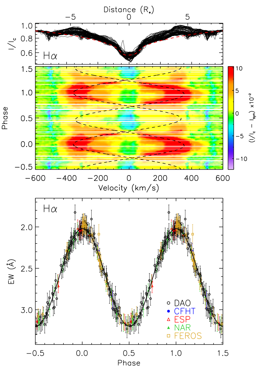
Figure 14: Top: Observed H$\alpha$ spectrum ($I/I_{c}$, solid black curve) compared with the average synthetic spectrum (dotted red). Middle: Dynamic spectra of $I/I_{c}-I_{\rm syn}$ where $I_{\rm syn}$ is the synthetic spectrum. A low-pass filter has been applied to the spectrum in order to minimize the A star contributions and tellurics. Bottom: Measured equivalent widths of H$\alpha$ using ESPaDOnS (open red triangles), Narval (filled green triangles), FEROS (yellow squares), CFHT f/8.2 spectrograph (filled blue circles), and DAO (open black circles) observations. The black curve indicates the best-fitting sinusoid. Both the EWs and dynamic spectra are phased by the B star’s rotational period of $0.853807\,{\rm d}$.

Given that the hot plasma surrounding HD 35502’s B star is co-rotating with the star at a distance of $\approx 4\,R_{\ast}$, i.e. between $R_{K}$ and $R_{\rm Alf}$, it is likely that the plasma is being confined by the strong magnetic field. Similar examples of magnetic B-type stars producing H emission well beyond the stellar radius (at distances of $\approx 2-4\,R_{\ast}$) have been previously reported (e.g. Bohlender & Monin, 2011; Oksala et al., 2012; Grunhut et al., 2012). In each of these cases, the star’s Alfvén radius exceeds its Kepler radius by approximately an order of magnitude (Petit et al., 2013; Shultz et al., 2014). Using the $R_{\rm Alf}$ value obtained from the $\langle B\rangle_{\rm H}$ measurements, we derived an $R_{\rm Alf}$ to $R_{K}$ ratio of $19^{+20}_{-5}$. Therefore, the fact that we observe strong H$\alpha$ emission is in agreement with this $R_{\rm Alf}/R_{K}\gtrsim 10$ empirical limit.

The magnetic confinement-rotation diagram compiled by Petit et al. (2013) allows $R_{K}$ and $R_{\rm Alf}$ to be understood within the broader context of all known O and B stars that host magnetospheres. Our characterization of the magnetosphere hosted by HD 35502’s B star suggests that it is well within the centrifugal magnetosphere regime. Only two other stars have been discovered exhibiting similar $R_{\rm Alf}$ and $R_{K}$ values within the derived $R_{\rm Alf}>40\,R_{\ast}$ and $1.5\leq R_{K}\leq 2.5\,R_{\ast}$. Although approximately four other stars have lower limits of $R_{\rm Alf}$ and $R_{K}$ that are consistent with HD 35502’s, only HD$\,182180$ (Rivinius et al., 2013) and HD$\,142184$ (Grunhut et al., 2012) have reported upper and lower uncertainties. These two examples have similar effective temperatures, surface gravities, radii, and masses to HD 35502’s magnetic B star. However, HD$\,182180$ and HD$\,142184$ are slightly faster rotators ($P_{\rm rot}\approx 0.5\,{\rm d}$) and host magnetic fields with weaker dipolar components ($B_{p}\approx 10\,{\rm kG}$).

Table 6: Magnetospheric parameters derived from $\langle B_{z}\rangle_{\rm H}$ and $\langle B_{z}\rangle_{\rm He+metal}$ measurements.

	HLSD	He+metalLSD
$i\,(\degree)$	$24^{+8}_{-9}$	$24^{+8}_{-9}$
$\beta\,(\degree)$	$63\pm 13$	$66^{+9}_{-13}$
$B_{p}\,{\rm(kG)}$	$14^{+9}_{-3}$	$15^{+10}_{-4}$
$\dot{M}_{B=0}\,(M_{\odot}\,{\rm yr}^{-1})$	$(1.3^{+6.0}_{-1.0})\times 10^{-10}$	$(1.3^{+6.0}_{-1.0})\times 10^{-10}$
$V_{\infty}\,({\rm km\,s}^{-1})$	$1100^{+40}_{-110}$	$1100^{+40}_{-110}$
$\eta_{\ast}$	$(2.6^{+7.9}_{-1.3})\times 10^{6}$	$(3.0^{+6.5}_{-1.5})\times 10^{6}$
$R_{\rm Alf}\,(R_{\ast})$	$41^{+17}_{-6}$	$42^{+14}_{-7}$
$R_{K}\,(R_{\ast})$	$2.1^{+0.4}_{-0.7}$	$2.1^{+0.4}_{-0.7}$
$R_{\rm Alf}/R_{K}$	$19^{+20}_{-5}$	$20^{+18}_{-6}$

8 Conclusion

The analysis presented here demonstrates a number of new discoveries regarding the nature of HD 35502. The high resolution spectroscopic and spectropolarimetric observations obtained using ESPaDOnS, Narval, and FEROS indicate that it is an SB3 system containing a central magnetic B-type star and two cooler A-type stars, all of which lie on the main sequence. We confirm that HD 35502’s speckle companion reported by Balega et al. (2012) is indeed the A star binary system. Our analysis indicates that both the A stars are physically nearly identical with a mass ratio of $1.05\pm 0.02$, masses of $2.1\,M_{\odot}$, and effective temperatures of $8.9\,{\rm kK}$.

Based on radial velocity measurements, we find that the two A stars form a binary system with an orbital period of $5.66866(6)\,{\rm d}$. No radial velocity variations of the B star were detected over the 22 year observing period, which can be explained by the inferred orbital period of $P_{\rm orb}\gtrsim 40\,{\rm yrs}$. However, two other explanations can account for the lack of detected radial velocity variations: (1) the inclination angle associated with the A star binary’s orbit about the B star may be $\sim 0\,\degree$ or (2) the A star binary may lie along the line of sight but not be gravitationally bound to the B star. A number of factors favour the triple system description such as the consistent flux ratios between the three components derived here. Specifically, if the two A stars are significantly closer or further than HD 35502’s $400\pm 80\,\rm{pc}$ distance, they would no longer lie on the main sequence. Furthermore, the radial velocity of the Orion OB1a subassociation, of which HD 35502 is most likely a member, has a reported velocity of $\approx 24\,{\rm km\,s}^{-1}$ (Morrell & Levato, 1991) and is therefore consistent with both the B star’s average radial velocity of $21\pm 2\,{\rm km\,s}^{-1}$ and the radial velocity of the A star binary’s center of mass ($27\pm 3\,{\rm km\,s}^{-1}$).

Our analysis of HD 35502’s central B star revealed the following:

1. it has an effective temperature of $18.4\,{\rm kK}$, a mass of $5.7\,M_{\odot}$, and a polar radius of $3.0\,R_{\odot}$;

2. it rotates relatively rapidly with a rotational period of $0.853807(3)\,{\rm d}$;

3. we detect a strong magnetic field and derive the magnitude of its dipolar component ($B_{p}\approx 14\,{\rm kG}$) and its obliquity ($\beta=63\,\degree$);

4. it exhibits significant line variability in the form of emission and chemical spots. The emission is predominantly observed in H$\alpha$ at a distance of approximately four times the stellar radius. Strong He abundance variations indicate a higher concentration near the negative pole of the magnetic field’s dipole component;

5. we derive an Alfvén and Kepler radii of $R_{\rm Alf}\approx 41\,R_{\ast}$ and $R_{K}\approx 2.1\,R_{\ast}$ unambiguously indicating that HD 35502’s B star hosts a large centrifugally supported magnetosphere.

Our analysis indicates that the ‘sn’ classification appearing in HD 35502’s historical B5IVsnp spectral type (Abt & Levato, 1977) is most likely related to the presence of the sharp-lined binary companion along with the strong H emission. We therefore propose that this system be reclassified as a B5IVpe+A+A system.

Stars hosting strongly emitting centrifugal magnetospheres can provide useful insights towards our understanding of both stellar winds and stellar magnetism. Therefore, it is important that these rare systems be studied in detail. While this particular class of magnetic stars is certainly growing, the number of confirmed examples are still insufficient to solve various outstanding issues. For instance, the inferred magnetospheric material densities of CM-hosting stars are largely inconsistent with currently predicted values (e.g. Rivinius et al., 2013; Townsend et al., 2013; Shultz et al., 2014). Moreover, testing the validity of theoretical models describing the physical nature of these magnetospheres (e.g. the Rigidly Rotating Magnetosphere model derived by Townsend & Owocki, 2005) requires detailed comparisons with a diversity of observations such as those recently carried out by Oksala et al. (2012, 2015).

We conclude that the strong variability – both in terms of $\langle B_{z}\rangle$ and the observed line variability – makes HD 35502 a favourable subject of a magnetic Doppler imaging analysis (Piskunov & Kochukhov, 2002). However, any attempt would require the three spectral components to be disentangled. Our orbital solution provides the necessary first step towards accomplishing this task.

Table 7: Longitudinal field measurements derived using the LSD profiles that were generated from the ESPaDOnS and Narval spectra. Columns 3 to 6 list $\langle B_{z}\rangle$ derived from H, He+metal, He, C, Si, and Fe LSD profiles. This table will appear only in the electronic version of the paper.

HJD	Instrument	$\langle B_{z}\rangle_{\rm H}$	$\langle B_{z}\rangle_{\rm He+metal}$	$\langle B_{z}\rangle_{\rm He}$	$\langle B_{z}\rangle_{\rm C}$	$\langle B_{z}\rangle_{\rm Si}$	$\langle B_{z}\rangle_{\rm Fe}$
		$({\rm kG})$	$({\rm kG})$	$({\rm kG})$	$({\rm kG})$	$({\rm kG})$	$({\rm kG})$
$2454702.138$	ESPaDOnS	$0.39\pm 0.30$	$-0.27\pm 0.19$	$-0.53\pm 0.35$	$-0.52\pm 0.60$	$0.32\pm 0.38$	$0.09\pm 0.57$
$2455849.677$	Narval	$-0.14\pm 0.26$	$0.12\pm 0.22$	$-0.96\pm 0.41$	$0.88\pm 0.60$	$1.91\pm 0.93$	$1.44\pm 0.65$
$2455893.623$	Narval	$-2.75\pm 0.32$	$-2.96\pm 0.27$	$-3.47\pm 0.48$	$-2.29\pm 0.80$	$-2.53\pm 0.61$	$-0.56\pm 0.88$
$2455910.518$	Narval	$-1.26\pm 0.74$	$-1.50\pm 0.55$	$-1.63\pm 1.04$	$-2.27\pm 1.60$	$0.17\pm 0.88$	$-1.15\pm 2.26$
$2455934.528$	Narval	$-2.27\pm 0.28$	$-2.86\pm 0.29$	$-3.51\pm 0.56$	$-2.64\pm 0.73$	$-6.63\pm 1.57$	$-0.57\pm 0.94$
$2455936.534$	Narval	$-2.04\pm 0.35$	$-2.21\pm 0.29$	$-2.93\pm 0.51$	$-1.27\pm 0.90$	$-3.25\pm 1.13$	$-2.82\pm 0.77$
$2455938.525$	Narval	$0.48\pm 0.32$	$-0.08\pm 0.25$	$-0.42\pm 0.45$	$0.11\pm 0.73$	$0.90\pm 0.54$	$1.83\pm 0.85$
$2455944.500$	Narval	$0.25\pm 0.37$	$0.30\pm 0.28$	$0.25\pm 0.53$	$1.05\pm 0.77$	$1.30\pm 0.54$	$1.94\pm 1.01$
$2455949.429$	Narval	$-0.89\pm 0.28$	$-1.09\pm 0.24$	$-1.69\pm 0.44$	$-1.36\pm 0.81$	$-1.08\pm 0.51$	$-1.19\pm 0.81$
$2455950.472$	Narval	$0.41\pm 0.40$	$-0.10\pm 0.31$	$-0.86\pm 0.60$	$0.03\pm 0.96$	$1.57\pm 0.69$	$0.51\pm 0.80$
$2455951.471$	Narval	$-0.62\pm 0.42$	$-1.37\pm 0.38$	$-2.03\pm 0.74$	$-1.34\pm 0.93$	$-1.18\pm 0.91$	$2.07\pm 0.95$
$2455966.376$	Narval	$-2.45\pm 0.36$	$-2.39\pm 0.24$	$-2.52\pm 0.41$	$-2.91\pm 0.78$	$-2.70\pm 0.57$	$-1.54\pm 0.64$
$2455998.332$	Narval	$0.01\pm 0.44$	$0.26\pm 0.33$	$0.01\pm 0.58$	$-0.10\pm 1.07$	$0.35\pm 0.60$	$1.85\pm 1.12$
$2455999.362$	Narval	$-1.56\pm 0.40$	$-2.18\pm 0.40$	$-3.01\pm 0.78$	$-1.84\pm 0.99$	$-2.86\pm 1.57$	$-0.45\pm 1.01$
$2456001.309$	Narval	$-2.95\pm 0.34$	$-2.71\pm 0.24$	$-3.18\pm 0.43$	$-3.03\pm 0.79$	$-2.86\pm 0.75$	$-1.58\pm 0.80$
$2456003.329$	Narval	$0.18\pm 0.29$	$-0.30\pm 0.25$	$-0.67\pm 0.44$	$0.28\pm 0.76$	$0.23\pm 0.55$	$0.05\pm 0.82$
$2456202.665$	Narval	$-2.78\pm 0.32$	$-2.97\pm 0.25$	$-3.75\pm 0.49$	$-3.26\pm 0.69$	$-3.15\pm 0.61$	$-1.24\pm 0.73$
$2456205.618$	Narval	$-0.51\pm 0.35$	$-0.51\pm 0.28$	$-1.21\pm 0.53$	$0.36\pm 0.76$	$0.68\pm 0.67$	$-1.44\pm 0.78$
$2456224.646$	Narval	$-0.43\pm 0.37$	$-0.09\pm 0.32$	$-0.26\pm 0.57$	$0.48\pm 1.08$	$-0.29\pm 0.58$	$0.92\pm 0.95$
$2456246.505$	Narval	$-1.88\pm 0.36$	$-1.55\pm 0.28$	$-2.19\pm 0.52$	$-1.83\pm 0.77$	$-1.15\pm 0.79$	$-1.30\pm 0.73$
$2456293.881$	ESPaDOnS	$-1.54\pm 0.30$	$-1.71\pm 0.26$	$-2.67\pm 0.56$	$-0.77\pm 0.62$	$-1.29\pm 0.70$	$0.11\pm 0.66$
$2456295.787$	ESPaDOnS	$-3.78\pm 1.05$	$-1.89\pm 0.73$	$-3.29\pm 1.19$	$0.76\pm 2.22$	$-4.78\pm 1.73$	$0.55\pm 2.74$
$2456295.808$	ESPaDOnS	$-3.07\pm 0.96$	$-2.58\pm 0.62$	$-2.71\pm 1.02$	$-3.48\pm 1.96$	$-2.35\pm 1.43$	$-1.95\pm 2.44$
$2456556.002$	ESPaDOnS	$-1.11\pm 0.47$	$-1.43\pm 0.30$	$-2.00\pm 0.55$	$-0.04\pm 0.87$	$-0.46\pm 0.50$	$0.49\pm 0.93$
$2456557.140$	ESPaDOnS	$-2.64\pm 0.39$	$-3.00\pm 0.25$	$-3.23\pm 0.44$	$-3.73\pm 0.76$	$-6.19\pm 1.16$	$-2.18\pm 0.69$
$2456560.077$	ESPaDOnS	$0.31\pm 0.40$	$0.27\pm 0.28$	$-0.23\pm 0.52$	$0.69\pm 0.83$	$1.48\pm 0.89$	$1.00\pm 0.65$

Table 8: Equivalent widths of H$\alpha$ calculated using all of the DAO, CFHT f/8.2 spectrograph, Narval, ESPaDOnS, and FEROS spectra. The uncertainties correspond to $3\sigma$. This table will appear only in the electronic version of the paper.

HJD	Instrument	${\rm EW_{H}}_{\alpha}$	HJD	Instrument	${\rm EW_{H}}_{\alpha}$
		$({\rm\AA})$			$({\rm\AA})$
$2448529.029$	DAO	$2.77\pm 0.10$	$2455910.518$	Narval	$2.66\pm 0.08$
$2448582.005$	CFHT f/8.2	$3.11\pm 0.09$	$2455934.528$	Narval	$2.28\pm 0.10$
$2448582.103$	CFHT f/8.2	$3.09\pm 0.09$	$2455936.534$	Narval	$2.49\pm 0.08$
$2448582.901$	CFHT f/8.2	$3.09\pm 0.09$	$2455938.525$	Narval	$3.14\pm 0.09$
$2448582.999$	CFHT f/8.2	$3.05\pm 0.09$	$2455944.500$	Narval	$3.16\pm 0.09$
$2448583.112$	CFHT f/8.2	$2.64\pm 0.08$	$2455949.429$	Narval	$2.84\pm 0.10$
$2448597.819$	DAO	$1.81\pm 0.10$	$2455950.472$	Narval	$3.11\pm 0.10$
$2449592.079$	CFHT f/8.2	$3.10\pm 0.10$	$2455951.471$	Narval	$2.77\pm 0.08$
$2449592.086$	CFHT f/8.2	$3.04\pm 0.10$	$2455953.653$	DAO	$2.66\pm 0.09$
$2449593.086$	CFHT f/8.2	$3.14\pm 0.09$	$2455953.663$	DAO	$2.74\pm 0.09$
$2449593.097$	CFHT f/8.2	$3.14\pm 0.09$	$2455953.674$	DAO	$2.76\pm 0.09$
$2449594.055$	CFHT f/8.2	$2.67\pm 0.08$	$2455953.684$	DAO	$2.82\pm 0.09$
$2449594.067$	CFHT f/8.2	$2.59\pm 0.09$	$2455953.695$	DAO	$2.85\pm 0.10$
$2449682.777$	DAO	$2.86\pm 0.09$	$2455953.705$	DAO	$2.90\pm 0.09$
$2449682.832$	DAO	$2.65\pm 0.09$	$2455953.716$	DAO	$2.97\pm 0.10$
$2449682.879$	DAO	$2.48\pm 0.09$	$2455953.726$	DAO	$3.00\pm 0.10$
$2449682.912$	DAO	$2.35\pm 0.10$	$2455953.737$	DAO	$3.00\pm 0.09$
$2449682.951$	DAO	$2.28\pm 0.10$	$2455953.748$	DAO	$3.05\pm 0.10$
$2449682.976$	DAO	$2.14\pm 0.10$	$2455953.758$	DAO	$3.06\pm 0.10$
$2449682.999$	DAO	$2.09\pm 0.11$	$2455953.769$	DAO	$3.04\pm 0.10$
$2449684.754$	DAO	$2.05\pm 0.11$	$2455953.779$	DAO	$3.04\pm 0.10$
$2449684.800$	DAO	$2.05\pm 0.10$	$2455953.790$	DAO	$3.13\pm 0.10$
$2449689.861$	DAO	$2.11\pm 0.11$	$2455959.683$	DAO	$2.88\pm 0.10$
$2449689.908$	DAO	$1.99\pm 0.10$	$2455959.694$	DAO	$2.90\pm 0.10$
$2449690.749$	DAO	$2.02\pm 0.10$	$2455959.704$	DAO	$2.88\pm 0.10$
$2449690.796$	DAO	$2.08\pm 0.10$	$2455959.715$	DAO	$2.92\pm 0.10$
$2449690.842$	DAO	$1.93\pm 0.11$	$2455959.725$	DAO	$2.96\pm 0.10$
$2449690.864$	DAO	$2.29\pm 0.09$	$2455959.736$	DAO	$2.79\pm 0.11$
$2449690.917$	DAO	$2.34\pm 0.08$	$2455960.660$	DAO	$3.00\pm 0.11$
$2449690.983$	DAO	$2.64\pm 0.09$	$2455960.670$	DAO	$3.04\pm 0.10$
$2449691.006$	DAO	$2.83\pm 0.10$	$2455960.681$	DAO	$3.04\pm 0.11$
$2450767.881$	DAO	$3.07\pm 0.10$	$2455960.691$	DAO	$3.06\pm 0.10$
$2450768.849$	DAO	$2.80\pm 0.09$	$2455960.702$	DAO	$3.06\pm 0.11$
$2454702.138$	ESPaDOnS	$3.15\pm 0.10$	$2455960.712$	DAO	$3.05\pm 0.10$
$2455565.739$	DAO	$1.92\pm 0.11$	$2455960.722$	DAO	$3.03\pm 0.11$
$2455565.785$	DAO	$2.02\pm 0.11$	$2455960.733$	DAO	$3.05\pm 0.10$
$2455569.801$	DAO	$2.80\pm 0.09$	$2455960.743$	DAO	$2.98\pm 0.11$
$2455570.807$	DAO	$2.24\pm 0.11$	$2455960.754$	DAO	$3.00\pm 0.10$
$2455571.815$	DAO	$2.02\pm 0.10$	$2455960.764$	DAO	$3.03\pm 0.11$
$2455602.737$	DAO	$2.68\pm 0.09$	$2455960.775$	DAO	$2.97\pm 0.10$
$2455849.677$	ESPaDOnS	$3.18\pm 0.10$	$2455960.789$	DAO	$3.00\pm 0.11$
$2455849.934$	DAO	$2.50\pm 0.08$	$2455960.799$	DAO	$2.88\pm 0.11$
$2455849.945$	DAO	$2.48\pm 0.08$	$2455961.644$	DAO	$2.97\pm 0.09$
$2455849.955$	DAO	$2.43\pm 0.09$	$2455961.654$	DAO	$2.84\pm 0.09$
$2455849.966$	DAO	$2.37\pm 0.08$	$2455966.376$	Narval	$2.31\pm 0.08$
$2455849.976$	DAO	$2.36\pm 0.09$	$2455998.332$	Narval	$3.10\pm 0.09$
$2455849.987$	DAO	$2.31\pm 0.09$	$2455999.362$	Narval	$2.46\pm 0.09$
$2455849.997$	DAO	$2.30\pm 0.09$	$2456001.309$	Narval	$2.07\pm 0.09$
$2455850.008$	DAO	$2.35\pm 0.09$	$2456003.329$	Narval	$3.16\pm 0.10$
$2455850.018$	DAO	$2.23\pm 0.10$	$2456191.654$	Narval	$2.08\pm 0.12$
$2455850.029$	DAO	$2.22\pm 0.10$	$2456202.665$	Narval	$2.15\pm 0.11$
$2455850.039$	DAO	$2.18\pm 0.10$	$2456205.618$	Narval	$3.05\pm 0.10$
$2455850.050$	DAO	$2.20\pm 0.10$	$2456224.646$	Narval	$2.99\pm 0.09$
$2455850.062$	DAO	$2.15\pm 0.10$	$2456246.505$	Narval	$2.68\pm 0.09$
$2455850.933$	DAO	$2.12\pm 0.10$	$2456293.881$	ESPaDOnS	$2.65\pm 0.08$
$2455850.943$	DAO	$2.17\pm 0.10$	$2456295.767$	ESPaDOnS	$2.02\pm 0.11$
$2455850.954$	DAO	$2.15\pm 0.10$	$2456295.787$	ESPaDOnS	$2.04\pm 0.11$
$2455850.964$	DAO	$2.09\pm 0.10$	$2456295.808$	ESPaDOnS	$2.03\pm 0.11$
$2455850.975$	DAO	$2.11\pm 0.09$	$2456556.002$	ESPaDOnS	$2.71\pm 0.08$
$2455850.985$	DAO	$2.14\pm 0.10$	$2456557.140$	ESPaDOnS	$2.09\pm 0.09$
$2455850.996$	DAO	$2.05\pm 0.09$	$2456560.077$	ESPaDOnS	$3.14\pm 0.09$
$2455851.006$	DAO	$2.06\pm 0.09$	$2456656.568$	FEROS	$3.08\pm 0.09$
$2455851.017$	DAO	$2.16\pm 0.09$	$2456656.609$	FEROS	$3.05\pm 0.09$
$2455851.027$	DAO	$2.16\pm 0.09$	$2456658.535$	FEROS	$2.29\pm 0.10$
$2455851.038$	DAO	$2.15\pm 0.08$	$2456658.542$	FEROS	$2.29\pm 0.10$
$2455851.048$	DAO	$2.23\pm 0.09$	$2456658.679$	FEROS	$2.00\pm 0.11$
$2455880.839$	DAO	$2.14\pm 0.11$	$2456658.683$	FEROS	$1.99\pm 0.10$
$2455880.850$	DAO	$2.18\pm 0.10$	$2456658.686$	FEROS	$1.94\pm 0.11$
$2455880.860$	DAO	$2.16\pm 0.10$	$2456658.690$	FEROS	$1.96\pm 0.10$
$2455880.871$	DAO	$2.20\pm 0.10$	$2456658.694$	FEROS	$1.99\pm 0.10$
$2455880.881$	DAO	$2.10\pm 0.10$	$2456658.701$	FEROS	$1.98\pm 0.10$
$2455880.892$	DAO	$2.22\pm 0.09$	$2456658.701$	FEROS	$1.98\pm 0.10$
$2455880.902$	DAO	$2.20\pm 0.09$	$2456658.709$	FEROS	$1.98\pm 0.10$
$2455880.913$	DAO	$2.26\pm 0.09$	$2456658.713$	FEROS	$2.00\pm 0.10$
$2455880.923$	DAO	$2.19\pm 0.09$	$2456658.763$	FEROS	$2.10\pm 0.09$
$2455880.933$	DAO	$2.25\pm 0.09$	$2456659.627$	FEROS	$2.16\pm 0.09$
$2455880.944$	DAO	$2.27\pm 0.09$	$2456659.671$	FEROS	$2.30\pm 0.09$
$2455880.954$	DAO	$2.32\pm 0.09$	$2456659.677$	FEROS	$2.33\pm 0.09$
$2455880.965$	DAO	$2.34\pm 0.08$	$2456659.681$	FEROS	$2.09\pm 0.11$
$2455880.975$	DAO	$2.42\pm 0.09$	$2456659.685$	FEROS	$2.40\pm 0.09$
$2455880.986$	DAO	$2.51\pm 0.09$	$2456659.689$	FEROS	$2.41\pm 0.08$
$2455880.996$	DAO	$2.44\pm 0.09$	$2456659.693$	FEROS	$2.39\pm 0.09$
$2455881.019$	DAO	$2.58\pm 0.08$	$2456659.697$	FEROS	$2.45\pm 0.09$
$2455881.029$	DAO	$2.62\pm 0.09$	$2456659.700$	FEROS	$2.42\pm 0.08$
$2455881.040$	DAO	$2.64\pm 0.09$	$2456659.708$	FEROS	$2.50\pm 0.09$
$2455893.623$	Narval	$2.06\pm 0.11$	$2456659.746$	FEROS	$2.66\pm 0.10$
$2455903.772$	DAO	$2.45\pm 0.10$	$2456660.614$	FEROS	$2.71\pm 0.09$
$2455903.782$	DAO	$2.48\pm 0.10$	$2456660.653$	FEROS	$2.88\pm 0.10$
$2455903.793$	DAO	$2.40\pm 0.10$	$2456660.724$	FEROS	$3.07\pm 0.10$
$2455903.803$	DAO	$2.33\pm 0.10$	$2456660.763$	FEROS	$3.14\pm 0.11$
$2455903.814$	DAO	$2.30\pm 0.10$	$2456660.801$	FEROS	$3.17\pm 0.10$

Table 9: Equivalent widths of various spectral lines calculated using the Narval, ESPaDOnS, and FEROS spectra. The uncertainties correspond to $3\sigma$. This table will appear only in the electronic version of the paper.

HJD	Instrument	EW${}_{\text{C\,{\sc ii}}\,\lambda 4267}$	EW${}_{\text{He\,{\sc i}}\,\lambda 4713}$	EW${}_{\text{Si\,{\sc iii}}\,\lambda 4553}$	EW${}_{\text{N\,{\sc ii}}\,\lambda 4643}$	${\rm EW_{H}}_{\beta}$	${\rm EW_{H}}_{\gamma}$
		$(\times 10\,{\rm\AA})$	$(\times 10\,{\rm\AA})$	$(\times 10\,{\rm\AA})$	$(\times 10\,{\rm\AA})$	$(\times 10\,{\rm\AA})$	$(\times 10\,{\rm\AA})$
$2454702.138$	ESPaDOnS	$1.53\pm 0.07$	$1.23\pm 0.05$	$0.89\pm 0.02$	$0.25\pm 0.01$	$59.38\pm 0.70$	$56.40\pm 0.67$
$2455849.677$	Narval	$1.49\pm 0.07$	$1.30\pm 0.05$	$0.84\pm 0.03$	$0.26\pm 0.01$	$58.36\pm 0.71$	$56.13\pm 0.69$
$2455893.623$	Narval	$1.47\pm 0.07$	$1.98\pm 0.06$	$0.78\pm 0.04$	$0.28\pm 0.02$	$56.84\pm 0.72$	$56.01\pm 0.69$
$2455910.518$	Narval	$1.46\pm 0.07$	$1.49\pm 0.05$	$1.00\pm 0.04$	$0.31\pm 0.02$	$57.59\pm 0.69$	$55.84\pm 0.67$
$2455934.528$	Narval	$1.49\pm 0.07$	$1.78\pm 0.06$	$0.87\pm 0.04$	$0.24\pm 0.02$	$57.09\pm 0.69$	$55.69\pm 0.65$
$2455936.534$	Narval	$1.50\pm 0.07$	$1.63\pm 0.06$	$0.78\pm 0.03$	$0.34\pm 0.02$	$57.33\pm 0.66$	$55.97\pm 0.65$
$2455938.525$	Narval	$1.50\pm 0.07$	$1.24\pm 0.04$	$0.81\pm 0.03$	$0.30\pm 0.01$	$58.16\pm 0.70$	$55.76\pm 0.67$
$2455944.500$	Narval	$1.50\pm 0.07$	$1.18\pm 0.05$	$0.84\pm 0.03$	$0.31\pm 0.01$	$58.23\pm 0.70$	$55.93\pm 0.67$
$2455949.429$	Narval	$1.55\pm 0.07$	$1.34\pm 0.05$	$0.85\pm 0.03$	$0.32\pm 0.02$	$58.42\pm 0.70$	$55.74\pm 0.67$
$2455950.472$	Narval	$1.51\pm 0.07$	$1.16\pm 0.05$	$0.93\pm 0.03$	$0.31\pm 0.02$	$58.64\pm 0.70$	$55.89\pm 0.67$
$2455951.471$	Narval	$1.51\pm 0.07$	$1.35\pm 0.05$	$0.98\pm 0.04$	$0.32\pm 0.01$	$58.15\pm 0.68$	$55.39\pm 0.67$
$2455966.376$	Narval	$1.54\pm 0.07$	$1.76\pm 0.06$	$0.68\pm 0.03$	$0.32\pm 0.02$	$57.45\pm 0.67$	$56.00\pm 0.65$
$2455998.332$	Narval	$1.47\pm 0.08$	$1.23\pm 0.04$	$0.87\pm 0.03$	$0.34\pm 0.02$	$58.02\pm 0.69$	$56.05\pm 0.66$
$2455999.362$	Narval	$1.50\pm 0.07$	$1.55\pm 0.05$	$0.87\pm 0.04$	$0.34\pm 0.02$	$56.27\pm 0.69$	$55.95\pm 0.67$
$2456001.309$	Narval	$1.51\pm 0.07$	$1.91\pm 0.06$	$0.75\pm 0.02$	$0.32\pm 0.02$	$56.69\pm 0.68$	$56.14\pm 0.65$
$2456003.329$	Narval	$1.54\pm 0.07$	$1.24\pm 0.05$	$0.79\pm 0.03$	$0.30\pm 0.02$	$58.24\pm 0.70$	$56.57\pm 0.66$
$2456191.654$	Narval	$1.51\pm 0.07$	$2.01\pm 0.06$	$0.78\pm 0.03$	$0.31\pm 0.02$	$56.86\pm 0.70$	$56.08\pm 0.66$
$2456202.665$	Narval	$1.50\pm 0.07$	$1.90\pm 0.06$	$0.84\pm 0.04$	$0.30\pm 0.02$	$56.72\pm 0.69$	$55.84\pm 0.67$
$2456205.618$	Narval	$1.54\pm 0.07$	$1.33\pm 0.05$	$0.89\pm 0.03$	$0.31\pm 0.02$	$57.91\pm 0.70$	$56.05\pm 0.67$
$2456224.646$	Narval	$1.49\pm 0.07$	$1.33\pm 0.04$	$0.92\pm 0.03$	$0.32\pm 0.02$	$57.88\pm 0.68$	$55.72\pm 0.67$
$2456246.505$	Narval	$1.55\pm 0.07$	$1.51\pm 0.06$	$0.81\pm 0.04$	$0.27\pm 0.02$	$57.70\pm 0.67$	$55.84\pm 0.65$
$2456293.881$	ESPaDOnS	$1.47\pm 0.07$	$1.49\pm 0.05$	$1.03\pm 0.03$	$0.30\pm 0.01$	$58.46\pm 0.68$	$56.06\pm 0.66$
$2456295.767$	ESPaDOnS	$1.53\pm 0.09$	$2.01\pm 0.08$	$0.80\pm 0.04$	$0.19\pm 0.07$	$57.20\pm 0.73$	$56.02\pm 0.68$
$2456295.787$	ESPaDOnS	$1.45\pm 0.08$	$1.97\pm 0.07$	$0.86\pm 0.03$	$0.43\pm 0.04$	$57.01\pm 0.71$	$56.34\pm 0.66$
$2456295.808$	ESPaDOnS	$1.49\pm 0.08$	$2.02\pm 0.07$	$0.85\pm 0.03$	$0.30\pm 0.03$	$56.44\pm 0.70$	$56.22\pm 0.67$
$2456556.002$	ESPaDOnS	$1.48\pm 0.07$	$1.46\pm 0.05$	$1.02\pm 0.03$	$0.25\pm 0.02$	$58.17\pm 0.68$	$56.18\pm 0.68$
$2456557.140$	ESPaDOnS	$1.52\pm 0.07$	$1.94\pm 0.06$	$0.92\pm 0.03$	$0.21\pm 0.01$	$57.91\pm 0.67$	$56.44\pm 0.67$
$2456560.077$	ESPaDOnS	$1.53\pm 0.07$	$1.19\pm 0.05$	$1.01\pm 0.03$	$0.21\pm 0.02$	$58.63\pm 0.70$	$56.34\pm 0.68$
$2456656.568$	FEROS	$1.55\pm 0.07$	$1.23\pm 0.05$	$0.81\pm 0.03$	$0.38\pm 0.02$	$58.40\pm 0.71$	$55.16\pm 0.66$
$2456656.609$	FEROS	$1.55\pm 0.07$	$1.15\pm 0.05$	$0.83\pm 0.03$	$0.33\pm 0.02$	$58.48\pm 0.72$	$55.15\pm 0.68$
$2456658.535$	FEROS	$1.50\pm 0.07$	$1.74\pm 0.06$	$0.70\pm 0.03$	$0.36\pm 0.02$	$57.26\pm 0.78$	$55.12\pm 0.68$
$2456658.542$	FEROS	$1.50\pm 0.08$	$1.81\pm 0.07$	$0.79\pm 0.04$	$0.30\pm 0.03$	$56.68\pm 0.73$	$55.32\pm 0.68$
$2456658.679$	FEROS	$1.50\pm 0.07$	$2.01\pm 0.07$	$0.65\pm 0.03$	$0.31\pm 0.03$	$57.00\pm 0.77$	$55.54\pm 0.68$
$2456658.683$	FEROS	$1.53\pm 0.07$	$2.04\pm 0.07$	$0.74\pm 0.03$	$0.35\pm 0.02$	$56.77\pm 0.75$	$55.49\pm 0.68$
$2456658.686$	FEROS	$1.51\pm 0.08$	$1.99\pm 0.07$	$0.69\pm 0.03$	$0.29\pm 0.02$	$56.81\pm 0.72$	$55.35\pm 0.67$
$2456658.690$	FEROS	$1.45\pm 0.07$	$1.91\pm 0.07$	$0.66\pm 0.02$	$0.30\pm 0.02$	$57.14\pm 0.82$	$55.47\pm 0.68$
$2456658.694$	FEROS	$1.46\pm 0.07$	$1.97\pm 0.07$	$0.66\pm 0.02$	$0.33\pm 0.02$	$56.74\pm 0.70$	$55.34\pm 0.66$
$2456658.698$	FEROS	$1.52\pm 0.07$	$1.91\pm 0.07$	$0.70\pm 0.02$	$0.33\pm 0.02$	$56.87\pm 0.71$	$55.40\pm 0.67$
$2456658.701$	FEROS	$1.51\pm 0.07$	$1.94\pm 0.07$	$0.68\pm 0.03$	$0.28\pm 0.02$	$56.93\pm 0.70$	$55.34\pm 0.66$
$2456658.702$	FEROS	$1.51\pm 0.07$	$1.99\pm 0.07$	$0.66\pm 0.03$	$0.35\pm 0.02$	$56.77\pm 0.72$	$55.36\pm 0.67$
$2456658.709$	FEROS	$1.46\pm 0.07$	$1.95\pm 0.06$	$0.68\pm 0.02$	$0.27\pm 0.02$	$56.76\pm 0.72$	$55.32\pm 0.68$
$2456658.713$	FEROS	$1.44\pm 0.08$	$1.94\pm 0.06$	$0.70\pm 0.02$	$0.31\pm 0.02$	$56.97\pm 0.71$	$55.43\pm 0.65$
$2456658.763$	FEROS	$1.55\pm 0.07$	$1.85\pm 0.06$	$0.63\pm 0.03$	$0.28\pm 0.02$	$57.23\pm 0.72$	$55.46\pm 0.67$
$2456659.628$	FEROS	$1.58\pm 0.07$	$1.79\pm 0.07$	$0.68\pm 0.04$	$0.30\pm 0.02$	$57.52\pm 0.74$	$55.33\pm 0.66$
$2456659.671$	FEROS	$1.56\pm 0.07$	$1.64\pm 0.07$	$0.70\pm 0.04$	$0.28\pm 0.02$	$57.43\pm 0.68$	$55.13\pm 0.66$
$2456659.677$	FEROS	$1.59\pm 0.07$	$1.58\pm 0.06$	$0.73\pm 0.03$	$0.33\pm 0.03$	$57.69\pm 0.70$	$55.26\pm 0.65$
$2456659.681$	FEROS	$1.56\pm 0.06$	$1.62\pm 0.07$	$0.74\pm 0.04$	$0.29\pm 0.03$	$57.62\pm 0.71$	$55.21\pm 0.65$
$2456659.685$	FEROS	$1.60\pm 0.07$	$1.56\pm 0.07$	$0.73\pm 0.04$	$0.28\pm 0.02$	$57.49\pm 0.69$	$55.55\pm 0.68$
$2456659.689$	FEROS	$1.58\pm 0.07$	$1.62\pm 0.07$	$0.77\pm 0.04$	$0.30\pm 0.02$	$57.77\pm 0.70$	$55.27\pm 0.64$
$2456659.693$	FEROS	$1.53\pm 0.08$	$1.51\pm 0.07$	$0.76\pm 0.04$	$0.29\pm 0.03$	$57.65\pm 0.70$	$55.16\pm 0.67$
$2456659.697$	FEROS	$1.60\pm 0.07$	$1.55\pm 0.07$	$0.75\pm 0.04$	$0.30\pm 0.03$	$57.58\pm 0.68$	$55.15\pm 0.66$
$2456659.700$	FEROS	$1.60\pm 0.07$	$1.57\pm 0.06$	$0.74\pm 0.04$	$0.29\pm 0.03$	$57.59\pm 0.69$	$55.25\pm 0.66$
$2456659.704$	FEROS	$1.53\pm 0.06$	$1.48\pm 0.07$	$0.76\pm 0.04$	$0.32\pm 0.02$	$57.75\pm 0.68$	$55.20\pm 0.65$
$2456659.708$	FEROS	$1.62\pm 0.07$	$1.54\pm 0.06$	$0.80\pm 0.04$	$0.29\pm 0.02$	$57.65\pm 0.69$	$55.05\pm 0.66$
$2456659.746$	FEROS	$1.59\pm 0.07$	$1.39\pm 0.06$	$0.78\pm 0.04$	$0.31\pm 0.02$	$58.13\pm 0.73$	$55.13\pm 0.66$
$2456660.614$	FEROS	$1.52\pm 0.07$	$1.50\pm 0.06$	$0.76\pm 0.03$	$0.32\pm 0.02$	$58.03\pm 0.76$	$55.16\pm 0.67$
$2456660.653$	FEROS	$1.55\pm 0.07$	$1.43\pm 0.05$	$0.78\pm 0.03$	$0.33\pm 0.02$	$58.04\pm 0.71$	$55.21\pm 0.68$
$2456660.724$	FEROS	$1.55\pm 0.07$	$1.29\pm 0.05$	$0.79\pm 0.03$	$0.27\pm 0.01$	$58.33\pm 0.74$	$55.25\pm 0.67$
$2456660.763$	FEROS	$1.54\pm 0.07$	$1.21\pm 0.05$	$0.75\pm 0.03$	$0.36\pm 0.02$	$58.34\pm 0.71$	$55.31\pm 0.69$
$2456660.801$	FEROS	$1.52\pm 0.07$	$1.22\pm 0.05$	$0.79\pm 0.03$	$0.33\pm 0.02$	$58.30\pm 0.74$	$55.37\pm 0.67$

Table 10: $uvby$ photometry obtained from Jan. 1992 to Mar. 1994. Each measurement is given as a magnitude difference between the variable source (“v”, HD 35502) and a non-variable comparison star (“c”, HD 35575). This table will appear only in the electronic version of the paper.

HJD	$u$(v-c)	$v$(v-c)	$b$(v-c)	$y$(v-c)	HJD	$u$(v-c)	$v$(v-c)	$b$(v-c)	$y$(v-c)
	(mag)	(mag)	(mag)	(mag)		(mag)	(mag)	(mag)	(mag)
$2448648.764$	$1.25$	$1.04$	$0.96$	$0.89$	$2449291.008$	$1.27$	$1.06$	$0.98$	$0.91$
$2448657.697$	$1.27$	$1.06$	$0.97$	$0.89$	$2449292.006$	$1.28$	$1.08$	$0.99$	$0.91$
$2448676.640$	$1.27$	$1.07$	$0.98$	$0.91$	$2449294.930$	$1.27$	$1.07$	$0.99$	$0.92$
$2448678.635$	$1.26$	$1.05$	$0.97$	$0.90$	$2449297.965$	$1.28$	$1.08$	$0.99$	$0.91$
$2448681.635$	$1.27$	$1.07$	$0.97$	$0.90$	$2449311.949$	$1.27$	$1.06$	$0.98$	$0.91$
$2448687.621$	$1.28$	$1.07$	$0.98$	$0.90$	$2449312.945$	$1.26$	$1.06$	$0.97$	$0.90$
$2448692.632$	$1.27$	$1.08$	$0.99$	$0.91$	$2449318.933$	$1.26$	$1.05$	$0.98$	$0.90$
$2448695.633$	$1.27$	$1.06$	$0.98$	$0.91$	$2449324.920$	$1.26$	$1.06$	$0.97$	$0.90$
$2448696.605$	$1.26$	$1.06$	$0.97$	$0.90$	$2449325.917$	$1.26$	$1.05$	$0.97$	$0.90$
$2448697.604$	$1.26$	$1.06$	$0.97$	$0.90$	$2449328.909$	$1.27$	$1.06$	$0.97$	$0.91$
$2448701.606$	$1.27$	$1.07$	$0.98$	$0.91$	$2449336.881$	$1.26$	$1.06$	$0.99$	$0.92$
$2448701.621$	$1.27$	$1.06$	$0.98$	$0.90$	$2449337.881$	$1.27$	$1.06$	$0.97$	$0.91$
$2448702.606$	$1.27$	$1.07$	$0.98$	$0.91$	$2449338.877$	$1.27$	$1.07$	$0.99$	$0.91$
$2448705.607$	$1.29$	$1.08$	$1.00$	$0.92$	$2449346.853$	$1.28$	$1.08$	$0.99$	$0.92$
$2448873.946$	$1.26$	$1.06$	$0.98$	$0.90$	$2449351.841$	$1.29$	$1.08$	$0.99$	$0.92$
$2448874.944$	$1.26$	$1.05$	$0.97$	$0.90$	$2449359.819$	$1.28$	$1.07$	$0.99$	$0.92$
$2448875.941$	$1.25$	$1.05$	$0.97$	$0.90$	$2449362.654$	$1.26$	$1.07$	$0.98$	$0.91$
$2448876.939$	$1.26$	$1.06$	$0.97$	$0.89$	$2449362.686$	$1.27$	$1.06$	$0.98$	$0.91$
$2448889.904$	$1.26$	$1.06$	$0.96$	$0.89$	$2449362.710$	$1.26$	$1.07$	$0.98$	$0.91$
$2448888.907$	$1.26$	$1.06$	$0.97$	$0.89$	$2449362.726$	$1.27$	$1.07$	$0.98$	$0.91$
$2448889.904$	$1.26$	$1.06$	$0.96$	$0.89$	$2449362.740$	$1.26$	$1.07$	$0.98$	$0.91$
$2448890.902$	$1.26$	$1.06$	$0.97$	$0.90$	$2449362.756$	$1.27$	$1.07$	$0.99$	$0.91$
$2448891.899$	$1.26$	$1.06$	$0.98$	$0.90$	$2449362.770$	$1.27$	$1.07$	$0.98$	$0.91$
$2448897.970$	$1.26$	$1.06$	$0.97$	$0.90$	$2449362.786$	$1.27$	$1.08$	$0.98$	$0.91$
$2448898.968$	$1.25$	$1.05$	$0.96$	$0.89$	$2449362.800$	$1.27$	$1.07$	$0.98$	$0.91$
$2448899.965$	$1.26$	$1.06$	$0.97$	$0.90$	$2449362.816$	$1.27$	$1.07$	$0.99$	$0.91$
$2448900.942$	$1.29$	$1.08$	$0.98$	$0.90$	$2449363.650$	$1.27$	$1.07$	$0.99$	$0.91$
$2448901.960$	$1.27$	$1.07$	$0.97$	$0.90$	$2449363.683$	$1.27$	$1.08$	$0.99$	$0.91$
$2448903.954$	$1.25$	$1.05$	$0.96$	$0.90$	$2449363.708$	$1.27$	$1.08$	$0.99$	$0.91$
$2448904.935$	$1.24$	$1.05$	$0.96$	$0.89$	$2449363.724$	$1.28$	$1.08$	$0.99$	$0.91$
$2448905.949$	$1.26$	$1.06$	$0.97$	$0.89$	$2449363.738$	$1.28$	$1.08$	$0.99$	$0.91$
$2448906.946$	$1.28$	$1.07$	$0.98$	$0.90$	$2449363.754$	$1.28$	$1.08$	$0.99$	$0.91$
$2448908.025$	$1.28$	$1.07$	$0.98$	$0.91$	$2449363.769$	$1.28$	$1.08$	$0.99$	$0.91$
$2448910.921$	$1.26$	$1.06$	$0.98$	$0.91$	$2449363.784$	$1.28$	$1.08$	$0.99$	$0.92$
$2448911.989$	$1.26$	$1.07$	$0.98$	$0.91$	$2449363.799$	$1.28$	$1.08$	$0.99$	$0.92$
$2448913.005$	$1.28$	$1.08$	$0.99$	$0.91$	$2449364.649$	$1.27$	$1.08$	$0.99$	$0.92$
$2448918.998$	$1.28$	$1.08$	$0.98$	$0.91$	$2449364.681$	$1.28$	$1.08$	$0.99$	$0.92$
$2448920.993$	$1.26$	$1.06$	$0.98$	$0.91$	$2449364.707$	$1.29$	$1.08$	$0.99$	$0.92$
$2448921.990$	$1.25$	$1.05$	$0.98$	$0.90$	$2449364.720$	$1.29$	$1.08$	$0.99$	$0.91$
$2448928.970$	$1.26$	$1.06$	$0.97$	$0.90$	$2449364.736$	$1.28$	$1.08$	$0.99$	$0.92$
$2448937.973$	$1.26$	$1.06$	$0.98$	$0.91$	$2449364.750$	$1.28$	$1.08$	$1.00$	$0.92$
$2448938.839$	$1.27$	$1.06$	$0.98$	$0.92$	$2449364.767$	$1.28$	$1.08$	$0.99$	$0.92$
$2448939.861$	$1.25$	$1.04$	$0.96$	$0.89$	$2449364.781$	$1.28$	$1.08$	$0.99$	$0.92$
$2448940.908$	$1.25$	$1.05$	$0.98$	$0.90$	$2449364.797$	$1.28$	$1.07$	$0.99$	$0.91$
$2448941.864$	$1.26$	$1.07$	$0.98$	$0.90$	$2449364.810$	$1.28$	$1.07$	$0.99$	$0.92$
$2448943.867$	$1.27$	$1.06$	$0.97$	$0.90$	$2449365.650$	$1.28$	$1.07$	$0.99$	$0.92$
$2448944.862$	$1.26$	$1.06$	$0.97$	$0.90$	$2449365.683$	$1.28$	$1.08$	$0.99$	$0.93$
$2448954.890$	$1.27$	$1.07$	$0.99$	$0.91$	$2449365.723$	$1.28$	$1.08$	$0.99$	$0.92$
$2448955.883$	$1.27$	$1.07$	$0.98$	$0.91$	$2449365.738$	$1.27$	$1.07$	$0.99$	$0.92$
$2448957.878$	$1.25$	$1.04$	$0.96$	$0.89$	$2449365.753$	$1.27$	$1.07$	$0.99$	$0.91$
$2448963.856$	$1.25$	$1.05$	$0.96$	$0.90$	$2449365.798$	$1.27$	$1.06$	$0.99$	$0.91$
$2448966.712$	$1.27$	$1.07$	$0.98$	$0.92$	$2449366.651$	$1.27$	$1.06$	$0.98$	$0.91$
$2448968.857$	$1.26$	$1.06$	$0.97$	$0.90$	$2449369.644$	$1.28$	$1.07$	$0.99$	$0.92$
$2449008.659$	$1.28$	$1.07$	$0.98$	$0.91$	$2449370.653$	$1.29$	$1.08$	$0.99$	$0.91$
$2449010.625$	$1.27$	$1.06$	$0.98$	$0.90$	$2449371.670$	$1.28$	$1.07$	$0.99$	$0.92$
$2449011.617$	$1.25$	$1.05$	$0.97$	$0.90$	$2449373.677$	$1.26$	$1.06$	$0.98$	$0.91$
$2449012.625$	$1.25$	$1.05$	$0.97$	$0.89$	$2449374.661$	$1.26$	$1.06$	$0.98$	$0.91$
$2449013.619$	$1.27$	$1.07$	$0.99$	$0.91$	$2449382.700$	$1.27$	$1.07$	$0.99$	$0.91$
$2449017.669$	$1.25$	$1.04$	$0.97$	$0.90$	$2449383.698$	$1.27$	$1.06$	$0.98$	$0.91$
$2449019.638$	$1.27$	$1.07$	$0.97$	$0.90$	$2449384.695$	$1.26$	$1.06$	$0.97$	$0.91$
$2449021.679$	$1.26$	$1.05$	$0.97$	$0.90$	$2449389.687$	$1.26$	$1.06$	$0.98$	$0.91$
$2449022.690$	$1.25$	$1.05$	$0.97$	$0.90$	$2449393.690$	$1.27$	$1.07$	$0.99$	$0.91$
$2449023.688$	$1.25$	$1.05$	$0.96$	$0.90$	$2449396.667$	$1.25$	$1.05$	$0.96$	$0.90$
$2449025.683$	$1.27$	$1.07$	$0.97$	$0.90$	$2449398.660$	$1.27$	$1.07$	$0.97$	$0.90$
$2449052.654$	$1.26$	$1.06$	$0.98$	$0.91$	$2449399.659$	$1.27$	$1.07$	$0.99$	$0.91$
$2449053.655$	$1.26$	$1.06$	$0.98$	$0.90$	$2449406.639$	$1.27$	$1.07$	$0.98$	$0.91$
$2449054.655$	$1.28$	$1.07$	$0.98$	$0.90$	$2449408.634$	$1.26$	$1.06$	$0.98$	$0.91$
$2449057.639$	$1.27$	$1.06$	$0.98$	$0.90$	$2449410.628$	$1.27$	$1.07$	$0.98$	$0.91$
$2449058.638$	$1.26$	$1.06$	$0.98$	$0.90$	$2449411.625$	$1.28$	$1.08$	$0.99$	$0.91$
$2449063.622$	$1.26$	$1.06$	$0.98$	$0.91$	$2449416.610$	$1.28$	$1.08$	$0.99$	$0.91$
$2449065.620$	$1.26$	$1.06$	$0.97$	$0.90$	$2449418.623$	$1.28$	$1.08$	$0.99$	$0.92$
$2449253.906$	$1.26$	$1.06$	$0.99$	$0.90$	$2449421.607$	$1.26$	$1.06$	$0.98$	$0.91$
$2449257.895$	$1.26$	$1.03$	$0.98$	$0.91$	$2449423.613$	$1.30$	$1.09$	$1.00$	$0.92$
$2449258.893$	$1.26$	$1.06$	$0.98$	$0.90$	$2449424.613$	$1.28$	$1.07$	$0.99$	$0.93$
$2449259.890$	$1.28$	$1.05$	$0.98$	$0.91$

References

• Abt & Hunter (1962) Abt H. A., Hunter J. H. J., 1962, ApJ, 136, 381
• Abt & Levato (1977) Abt H. A., Levato H., 1977, PASP, 89, 797
• Alecian et al. (2015) Alecian E. et al., 2015, in IAU Symp. 307, Meynet G., Georgy C., Groh J., Stee P., eds., Vol. 307, Geneva, Switzerland, pp. 330–335
• Balega et al. (2012) Balega Y. Y., Dyachenko V. V., Maksimov a. F., Malogolovets E. V., Rastegaev D. a., Romanyuk I. I., 2012, Astrophys. Bull., 67, 44
• Bohlender & Monin (2011) Bohlender D. A., Monin D., 2011, AJ, 141, 169
• Bolton et al. (1998) Bolton C. T., Harmanec P., Lyons R. W., Odell A. P., Pyper D. M., 1998, A&A, 337, 183
• Borra (1981) Borra E. F., 1981, ApJ, 249, L39
• Borra, Landstreet & Thompson (1983) Borra E. F., Landstreet J. D., Thompson I., 1983, ApJS, 53, 151
• Brown, de Geus & de Zeeuw (1994) Brown A. G. A., de Geus E. J., de Zeeuw P. T., 1994, A&A, 289, 101
• Bychkov, Bychkova & Madej (2005) Bychkov V. D., Bychkova L. V., Madej J., 2005, A&A, 430, 1143
• Cardelli, Clayton & Mathis (1989) Cardelli J. A., Clayton G. C., Mathis J. S., 1989, ApJ, 345, 245
• Carnochan (1982) Carnochan D. J., 1982, MNRAS, 201, 1139
• Castelli & Kurucz (2004) Castelli F., Kurucz R. L., 2004, ArXiv Astrophysics e-prints
• Cohen, Wheaton & Megeath (2003) Cohen M., Wheaton W. A., Megeath S. T., 2003, AJ, 126, 1090
• Crawford (1958) Crawford D. L., 1958, ApJ, 128, 185
• Donati et al. (1997) Donati J.-F., Semel M., Carter B. D., Rees D. E., Cameron A. C., 1997, MNRAS, 291, 658
• Ekström et al. (2012) Ekström S. et al., 2012, A&A, 537, 1
• Georgy et al. (2013) Georgy C., Ekström S., Granada a., Meynet G., Mowlavi N., Eggenberger P., Maeder a., 2013, A&A, 553, 1
• Glagolevskij et al. (2010) Glagolevskij Y. V., Chountonov G. A., Shavrina A. V., Pavlenko Y. V., 2010, Astrophysics, 53, 133
• Grunhut et al. (2012) Grunhut J. H. et al., 2012, MNRAS, 419, 1610
• Hareter et al. (2008) Hareter M. et al., 2008, A&A, 492, 185
• Horch et al. (2001) Horch E., van Altena W. F., M. G. T., Franz O. G., López C. E., Timothy J. G., 2001, AJ, 121, 1597
• Howarth (2011) Howarth I. D., 2011, MNRAS, 413, 1515
• Hubrig et al. (2015) Hubrig S. et al., 2015, A&A, 3, 1
• Kaufer et al. (1999) Kaufer A., Stahl O., Tubbesing S., Nørregaard P., Avila G., Francois P., Pasquini L., Pizzella A., 1999, The Messenger, 95, 8
• Kochukhov (2007) Kochukhov O., 2007, in Phys. Magn. Stars, pp. 109–118
• Kochukhov, Makaganiuk & Piskunov (2010) Kochukhov O., Makaganiuk V., Piskunov N., 2010, A&A, 524, 1
• Kochukhov et al. (2015) Kochukhov O., Rusomarov N., Valenti J. A., Stempels H. C., Snik F., Rodenhuis M., Piskunov N., 2015, A&A, 574, 1
• Krtička et al. (2009) Krtička J., Mikulášek Z., Henry G. W., Zverko J., Žižovský J., Skalický J., Zvěřina P., 2009, A&A, 499, 567
• Kupka et al. (2000) Kupka F. G., Ryabchikova T. A., Piskunov N. E., Stempels H. C., Weiss W. W., 2000, Balt. Astron., 9, 590
• Kurucz (1993) Kurucz R., 1993, ATLAS9 Stellar Atmosphere Programs and 2 km/s grid. Kurucz CD-ROM No. 13.  Cambridge, Mass.: Smithsonian Astrophysical Observatory, 1993., 13
• Landstreet et al. (2007) Landstreet J. D., Bagnulo S., Andretta V., Fossati L., Mason E., Silaj J., Wade G. A., 2007, A&A, 698, 685
• Landstreet et al. (2015) Landstreet J. D., Bagnulo S., Valyavin G. G., Gadelshin D., Martin a. J., Galazutdinov G., Semenko E., 2015, A&A, 580
• Landstreet & Borra (1978) Landstreet J. D., Borra E. F., 1978, ApJ, 224, L5
• Lee (1968) Lee T. A., 1968, ApJ, 152
• Leone et al. (2010) Leone F., Bohlender D. a., Bolton C. T., Buemi C., Catanzaro G., Hill G. M., Stift M. J., 2010, MNRAS, 401, 2739
• Monin et al. (2012) Monin D., Bohlender D., Hardy T., Saddlemyer L., Fletcher M., 2012, PASP, 124, 329
• Morrell & Levato (1991) Morrell N., Levato H., 1991, ApJS, 75, 965
• Neiner et al. (2003) Neiner C. et al., 2003, A&A, 411, 565
• Nissen (1976) Nissen P. E., 1976, A&A, 50, 343
• Oksala et al. (2015) Oksala M. E. et al., 2015, MNRAS, 451, 2015
• Oksala et al. (2010) Oksala M. E., Wade G. a., Marcolino W. L. F., Grunhut J., Bohlender D., Manset N., Townsend R. H. D., MiMe S. C., 2010, MNRAS, 405, L51
• Oksala et al. (2012) Oksala M. E., Wade G. A., Townsend R. H. D., Owocki S. P., Kochukhov O., Neiner C., Alecian E., Grunhut J., 2012, MNRAS, 419, 959
• Perryman et al. (1997) Perryman M. A. C. et al., 1997, A&A, 323, L49
• Petit et al. (2013) Petit V. et al., 2013, MNRAS, 429, 398
• Piskunov & Kochukhov (2002) Piskunov N., Kochukhov O., 2002, A&A, 381, 736
• Preston (1967) Preston G. W., 1967, ApJ, 150, 547
• Rivinius et al. (2013) Rivinius T., Townsend R. H. D., Kochukhov O., Stefl S., Baade D., Barrera L., Szeifert T., 2013, MNRAS, 429, 177
• Rufener (1981) Rufener F., 1981, A&AS, 45, 207
• Rufener & Nicolet (1988) Rufener F., Nicolet B., 1988, A&A, 206, 357
• Sharpless (1952) Sharpless S., 1952, ApJ, 116, 251
• Shore et al. (1990) Shore S. N., Brown D. N., Sonneborn G., Landstreet J. D., Bohlender D. A., 1990, ApJ, 348, 242
• Shultz et al. (2015) Shultz M., Rivinius T., Folsom C. P., Wade G. a., Townsend R. H. D., Sikora J., Grunhut J., Stahl O., 2015, MNRAS, 449, 3945
• Shultz et al. (2014) Shultz M., Wade G., Rivinius T., Townsend R., 2014, ASP Conf. Ser., 1
• Sikora et al. (2015) Sikora J. et al., 2015, MNRAS, 451, 1928
• Silvester et al. (2012) Silvester J., Wade G. A., Kochukhov O., Bagnulo S., Folsom C. P., Hanes D., 2012, MNRAS, 426, 1003
• Skrutskie et al. (2006) Skrutskie M. F. et al., 2006, AJ, 131, 1163
• Stibbs (1950) Stibbs D. W. N., 1950, MNRAS, 110, 395
• Thompson et al. (1978) Thompson G. I., Nandy K., Jamar C., Monfils A., Houziaux L., Carnochan D. J., Wilson R., 1978, Catalogue of Stellar Ultraviolet Fluxes (TD-1).
• Tokovinin (1992) Tokovinin A., 1992, in IAU Colloq. 135, McAlister H. A., Hartkopf W. I., eds., Vol. 32, ASP Conference Series, Moscow, Russia, pp. 573–576
• Townsend & Owocki (2005) Townsend R. H. D., Owocki S. P., 2005, MNRAS, 357, 251
• Townsend, Owocki & Groote (2005) Townsend R. H. D., Owocki S. P., Groote D., 2005, ApJ, 630, 81
• Townsend et al. (2013) Townsend R. H. D. et al., 2013, ApJ, 769, 33
• ud-Doula & Owocki (2002) ud-Doula A., Owocki S. P., 2002, ApJ, 576, 413
• ud-Doula, Owocki & Townsend (2008) ud-Doula A., Owocki S. P., Townsend R. H. D., 2008, MNRAS, 385, 97
• ud-Doula, Townsend & Owocki (2006) ud-Doula A., Townsend R. H. D., Owocki S. P., 2006, ApJ, 640, L191
• van Hamme (1993) van Hamme W., 1993, AJ, 106, 2096
• van Leeuwen (2007) van Leeuwen F., 2007, A&A, 474, 653
• Vink, de Koter & Lamers (2000) Vink J. S., de Koter A., Lamers H. J. G. L. M., 2000, A&A, 362, 295
• von Zeipel (1924) von Zeipel H., 1924, MNRAS, 84, 684
• Wade et al. (2000) Wade G. A., Donati J.-F., Landstreet J. D., Shorlin S. L. S., 2000, MNRAS, 313, 851
• Wade et al. (2012) Wade G. A. et al., 2012, MNRAS, 419, 2459
• Wade et al. (2015) Wade G. A. et al., 2015, MNRAS, 456, 2
• Walborn & Hesser (1976) Walborn N. R., Hesser J. E., 1976, ApJ, 205, L87
• Wall & Jenkins (2003) Wall J., Jenkins C., 2003, Practical Statistics for Astronomers, Cambridge Observing Handbooks for Research Astronomers. Cambridge University Press
• Wright et al. (2010) Wright E. L. et al., 2010, AJ, 140
• Yakunin et al. (2015) Yakunin I. et al., 2015, MNRAS, 447, 1418