Lectures on Integrable probability:
Stochastic vertex models and symmetric functions

Abstract.

We consider a homogeneous stochastic higher spin six vertex model in a quadrant. For this model we derive concise integral representations for multi-point $q$-moments of the height function and for the $q$-correlation functions. At least in the case of the step initial condition, our formulas degenerate in appropriate limits to many known formulas of such type for integrable probabilistic systems in the (1+1)d KPZ universality class, including the stochastic six vertex model, ASEP, various $q$-TASEPs, and associated zero range processes.

Our arguments are largely based on properties of a family of symmetric rational functions (introduced in [Bor14]) that can be defined as partition functions of the higher spin six vertex model for suitable domains; they generalize classical Hall–Littlewood and Schur polynomials. A key role is played by Cauchy-like summation identities for these functions, which are obtained as a direct corollary of the Yang–Baxter equation for the higher spin six vertex model.

These are lecture notes for a course given by A. B. at the Ecole de Physique des Houches in July of 2015. All the results and proofs presented here generalize to the setting of the fully inhomogeneous higher spin six vertex model, see [BP16] for a detailed exposition of the inhomogeneous case.

1. Introduction

1.1. Preface

The last two decades have seen remarkable progress in understanding the so-called KPZ universality class in (1+1) dimensions. This is a rather broad and somewhat vaguely defined class of probabilistic systems describing random interface growth, named after a seminal physics paper of Kardar–Parisi–Zhang of 1986 [KPZ86]. A key conjectural property of the systems in this class is that the large time fluctuations of the interfaces should be the same for all of them. See Corwin [Cor12] for an extensive survey.

While proving such a universality principle remains largely out of reach, by now many concrete systems have been found, for which the needed asymptotics was actually computed (the universality principle appears to hold so far).

The first wave of these solved systems started in late 1990’s with the papers of Johansson [Joh01] and Baik–Deift–Johansson [BDJ99], and the key to their solvability, or integrability, was in (highly non-obvious) reductions to what physicists would call free-fermion models — probabilistic systems, many of whose observables are expressed in terms of determinants and Pfaffians. Another domain where free-fermion models are extremely important is Random Matrix Theory. Perhaps not surprisingly, the large time fluctuations of the (1+1)d KPZ models are very similar to those arising in (largest eigenvalues of) random matrices with real spectra.

The second wave of integrable (1+1)d KPZ systems started in late 2000’s. The reasons for their solvability are harder to see, but one way or another they can be traced to quantum integrable systems. For example, looking at the earlier papers of the second wave we see that: (a) The pioneering work of Tracy–Widom [TW08], [TW09a], [TW09b] on the Asymmetric Simple Exclusion Process (ASEP) was based on the famous idea of Bethe [Bet31] of looking for eigenfunctions of a quantum many-body system in the form of superposition of those for noninteracting bodies (coordinate Bethe ansatz); (b) The work of O’Connell [O’C12] and Borodin–Corwin [BC14] on semi-discrete Brownian polymers utilized properties of eigenfunctions of the Macdonald–Ruijsenaars quantum integrable system — the celebrated Macdonald polynomials and their degenerations; (c) The physics papers of Dotsenko [Dot10] and Calabrese–Le Doussal–Rosso [CLDR10], and a later work of Borodin–Corwin–Sasamoto [BCS14] used a duality trick to show that certain observables of infinite-dimensional models solve finite-dimensional quantum many-body systems that are, in their turn, solvable by the coordinate Bethe ansatz; etc.

In fact, most currently known integrable (1+1)d KPZ models of the second wave come from one and the same quantum integrable system: Corwin–Petrov [CP16] recently showed that they can be realized as suitable limits of what they called a stochastic higher spin vertex model, see the introduction to their paper for a description of degenerations. They used duality and coordinate Bethe ansatz to show the integrability of their model; the Bethe ansatz part relied on previous works of Borodin–Corwin–Petrov–Sasamoto [BCPS15b], [BCPS15a], and Borodin [Bor14].

The main subject of the present paper is exactly that higher spin six vertex model. Our main result is an integral representation for certain multi-point $q$-moments of this model. Such formulas are well known to be a source of meaningful asymptotic results, but we leave asymptotic questions outside of the scope of these lectures.

The results and the proofs presented in these notes generalize to the setting of the fully inhomogeneous higher spin six vertex model; those are presented in our recent work [BP16].

The core of our proofs consists of the so-called (skew) Cauchy identities for certain rational symmetric functions which were introduced in [Bor14]. For special parameter values, these functions turn into (skew) Hall–Littlewood and Schur symmetric functions, and the name ‘‘Cauchy identities’’ is borrowed from the theory of those, cf. Macdonald [Mac95].

Our symmetric rational functions can be defined as partition functions of the higher spin six vertex model for domains with special boundary conditions. Following [Bor14], we use the Yang–Baxter equation, or rather its infinite-volume limit, to derive the Cauchy identities. A similar approach to Cauchy-like identities for the Hall–Littlewood polynomials was also realized by Wheeler–Zinn–Justin in [WZJ15].

Remarkably, the Cauchy identities themselves are essentially sufficient to define our probabilistic models, show their connection to KPZ interfaces, prove orthogonality and completeness of our symmetric rational functions, and evaluate averages of a large family of observables with respect to our measures. The last bit can be derived from comparing Cauchy identities with different sets of parameters.

While the Cauchy identities also played an important role in the theory of Schur and Macdonald processes, they were never the main heroes there. Here they really take the central stage. Given their direct relation to the Yang–Baxter equation, one could thus say that the integrability of the (1+1)d KPZ models takes its origin in the Yang–Baxter integrability of the six vertex model.

Our present approach circumvents the duality trick that has been so powerful in treating the integrable (1+1)d KPZ models (including that of [CP16]). We do explain how the duality can be discovered from our results, but we do not prove or rely on it. Unfortunately, for the moment the use and success of the duality approach remains somewhat mysterious and ad hoc; the form of the duality functional needs to be guessed from previously known examples (some of which have better explanations, cf. Schütz [Sch97], Borodin–Corwin [BC13]). We hope that the path that we present here is more straightforward, and that it can be used to shed further light on the existence of nontrivial dualities.

Let us now describe our results in more detail.

1.2. Our model in a quadrant

Consider an ensemble $\mathcal{P}$ of infinite oriented up-right paths drawn in the first quadrant $\mathbb{Z}_{\geq 1}^{2}$ of the square lattice, with all the paths starting from a left-to-right arrow entering at each of the points $\{(1,m):m\in\mathbb{Z}_{\geq 1}\}$ on the left boundary (no path enters through the bottom boundary). Assume that no two paths share any horizontal piece (but common vertices and vertical pieces are allowed). See Fig. 1.

Figure 1. A path collection $\mathcal{P}$.

Define a probability measure on the set of such path ensembles in the following Markovian way. For any $n\geq 2$, assume that we already have a probability distribution on the intersections $\mathcal{P}_{n}$ of $\mathcal{P}$ with the triangle $T_{n}=\{(x,y)\in\mathbb{Z}_{\geq 1}^{2}:x+y\leq n\}$. We are going to increase $n$ by 1. For each point $(x,y)$ on the upper boundary of $T_{n}$, i.e., for $x+y=n$, every $\mathcal{P}_{n}$ supplies us with two inputs: (1) The number of paths that enter $(x,y)$ from the bottom — denote it by $i_{1}\in\mathbb{Z}_{\geq 0}$; (2) The number of paths $j_{1}\in\{0,1\}$ that enter $(x,y)$ from the left. Now choose, independently for all $(x,y)$ on the upper boundary of $T_{n}$, the number of paths $i_{2}$ that leave $(x,y)$ in the upward direction, and the number of paths $j_{2}$ that leave $(x,y)$ in the rightward direction, using the probability distribution with weights of the transitions $(i_{1},j_{1})\to(i_{2},j_{2})$ given by (throughout the text $\mathbf{1}_{A}$ stands for the indicator function of the event $A$)

$$\begin{array}[]{rclrcl}\mathsf{Prob}((i_{1},0)\to(i_{2},0))=&\dfrac{1-q^{i_{1}}su_{y}}{1-su_{y}}\,\mathbf{1}_{i_{1}=i_{2}},\\ \rule{0.0pt}{22.0pt}\mathsf{Prob}((i_{1},0)\to(i_{2},1))=&\dfrac{(q^{i_{1}}-1)su_{y}}{1-su_{y}}\,\mathbf{1}_{i_{1}=i_{2}+1},\\ \rule{0.0pt}{22.0pt}\mathsf{Prob}((i_{1},1)\to(i_{2},1))=&\dfrac{s^{2}q^{i_{1}}-su_{y}}{1-su_{y}}\,\,\mathbf{1}_{i_{1}=i_{2}},\\ \rule{0.0pt}{22.0pt}\mathsf{Prob}((i_{1},1)\to(i_{2},0))=&\dfrac{1-s^{2}q^{i_{1}}}{1-su_{y}}\,\mathbf{1}_{i_{1}=i_{2}-1}.\end{array}$$ (1.5)

Assuming that all above expressions are nonnegative, which happens e.g. if $q\in(0,1)$, $u_{y}>0$, $s\in(-1,0)$, this procedure defines a probability measure on the set of all $\mathcal{P}$’s because we always have $\sum_{i_{2},j_{2}}\mathsf{Prob}((i_{1},j_{1})\to(i_{2},j_{2}))=1$, and $\mathsf{Prob}((i_{1},j_{1})\to(i_{2},j_{2}))$ vanishes unless $i_{1}+j_{1}=i_{2}+j_{2}$.

The right-hand sides in (1.5) are closely related to matrix elements of the R-matrix for $U_{q}(\widehat{\mathfrak{sl}_{2}})$, with one representation being an arbitrary Verma module and the other one being tautological.

Parameter $s$ is related to the value of the spin. If $s^{2}=q^{-I}$ for a positive integer $I$, then we have $\mathsf{Prob}((I,1)\to(I+1,0))=0$, which means that no more than $I$ paths can share the same vertical piece. This corresponds to replacing the arbitrary Verma module in the R-matrix with its $(I+1)$-dimensional irreducible quotient. The spin $\frac{1}{2}$ situation $s=q^{-\frac{1}{2}}$ gives rise to the stochastic six vertex introduced over 20 years ago by Gwa–Spohn [GS92] (see [BCG16] for its detailed treatment).

The spin parameter $s$ is related to columns, and there is no similar row parameter: recall that no two paths can share the same horizontal piece. This restriction can be repaired using the procedure of fusion that goes back to [KRS81]. In plain words, fusion means grouping the spectral parameters $\{u_{y}\}$ into subsequences of the form $\{u,qu,\dots,q^{J-1}u\}$, and collapsing the corresponding $J$ rows onto a single one. Here the positive integer $J$ plays the same role as $I$ in the previous paragraph. The reason we did not use the second spin parameter in (1.5) is that the transition probabilities then become rather cumbersome, and one needs to specialize other parameters to achieve simpler expressions. A detailed exposition of the fusion is contained in §5 below.

Let us also note that there are several substantially different possibilities of making the weights (1.5) nonnegative; some of those we consider in detail. Since our techniques are algebraic, our results actually apply to any generic parameter values, with typically only minor modifications needed in case of some denominators vanishing.

1.3. The main result

Encode each path ensemble $\mathcal{P}$ by a height function $\mathfrak{h}:\mathbb{Z}_{\geq 1}^{2}\to\mathbb{Z}_{\geq 0}$ which assigns to each vertex $(x,y)$ the number $\mathfrak{h}(x,y)$ of paths in $\mathcal{P}$ that pass through or to the right of this vertex.

Theorem (Theorem 9.8 in the text).

Assume that $q\in(0,1)$, $s\in(-1,0)$, $u_{y}>0$ for all $y\in\mathbb{Z}_{\geq 1}$, and $u_{i}\neq qu_{j}$ for any $i,j\geq 1$. Then for any integers $x_{1}\geq\ldots\geq x_{\ell}\geq 1$ and $y\geq 1$,

$$\operatorname{\mathbb{E}}\prod_{i=1}^{\ell}q^{\mathfrak{h}(x_{i},y)}=q^{\frac{\ell(\ell-1)}{2}}\oint\limits_{{\boldsymbol{\gamma}}[\bar{\mathbf{u}}|{1}]}\frac{dw_{1}}{2\pi\mathbf{i}}\ldots\oint\limits_{{\boldsymbol{\gamma}}[\bar{\mathbf{u}}|{\ell}]}\frac{dw_{\ell}}{2\pi\mathbf{i}}\prod_{1\leq{\upalpha}<{\upbeta}\leq\ell}\frac{w_{\upalpha}-w_{\upbeta}}{w_{\upalpha}-qw_{\upbeta}}\\ \times\prod_{i=1}^{\ell}\bigg{(}w_{i}^{-1}\left(\frac{1-sw_{i}}{1-s^{-1}w_{i}}\right)^{x_{i}-1}\prod_{j=1}^{y}\frac{1-qu_{j}w_{i}}{1-u_{j}w_{i}}\bigg{)},$$ (1.6)

where the expectation is taken with respect to the probability measure defined in §1.2 above, and the integration contours are described in Definitions 8.12 and 9.4 and pictured in Fig. 26 below.

Let us emphasize that the inequalities on the parameters here are exceedingly restrictive; the statement can be analytically continued with suitable modifications of the contours and the integrand. Examples of such analytic continuation can be found in §10, where they are used to degenerate the above result to various $q$-versions of the T(otally)ASEP.

We also prove integral formulas similar to (1.6) for another set of observables of our model that we call $q$-correlation functions. The two are related, but in a rather nontrivial way, and one set of formulas does not immediately imply the other.

While at the moment averages (1.6) seem more useful for asymptotic analysis (and that is the reason we list them as our main result), it is entirely possible that the $q$-correlation functions will become useful for other asymptotic regimes. The definition and the expressions for the $q$-correlation functions can be found in §8 below.

1.4. Symmetric rational functions

One consequence of the Yang–Baxter integrability of our model is that one can explicitly compute the distribution of intersection points of the paths in $\mathcal{P}$ with any horizontal line. More exactly, let $X_{1}\geq\ldots\geq X_{n}\geq 1$ be the $x$-coordinates of the points where our paths intersect the line $y=const$ with $n<const<n+1$; there are exactly $n$ of those, counting the multiplicities. Then

$$\mathsf{Prob}\{X_{1}=\nu_{1}+1,\dots,X_{n}=\nu_{n}+1\}=\prod_{k\geq 0}\frac{(-s)^{n_{k}}(s;q)_{n_{k}}}{(q;q)_{n_{k}}}\cdot\mathsf{F}_{\nu}(u_{1},\dots,u_{n}),$$ (1.7)

where $(a;q)_{m}=(1-a)(1-aq)\ldots(1-aq^{m-1})$ are the $q$-Pochhammer symbols, $n_{k}$ is the multiplicity of $k$ in the sequence $\nu=(\nu_{1}\geq\ldots\geq\nu_{n})=0^{n_{0}}1^{n_{1}}\cdots$, and for any $\mu=(\mu_{1}\geq\dots\geq\mu_{M}\geq 0)$ we define

$$\mathsf{F}_{\mu}(u_{1},\ldots,u_{M})=\frac{(1-q)^{M}}{\prod_{i=1}^{M}(1-su_{i})}\sum_{\sigma\in\mathfrak{S}_{M}}\sigma\Bigg{(}\prod_{1\leq{\upalpha}<{\upbeta}\leq M}\frac{u_{\upalpha}-qu_{\upbeta}}{u_{\upalpha}-u_{\upbeta}}\,\prod_{i=1}^{M}\left(\frac{u_{i}-s}{1-su_{i}}\right)^{\mu_{i}}\Bigg{)}.$$ (1.8)

Here $\mathfrak{S}_{M}$ is the symmetric group of degree $M$, and its elements $\sigma$ permute the variables $\{u_{i}\}_{i=1}^{M}$ in the right-hand side of (1.8).

The symmetric rational functions $\{\mathsf{F}_{\mu}\}$ play a central role in our work. The right-hand side of (1.8) can be viewed as a coordinate Bethe ansatz expression for the eigenfunctions of the transfer-matrix of the higher spin six vertex model. Note that one would need to additionally impose Bethe equations on the $u$’s for periodic in the $x$-direction boundary conditions.

The probabilistic interpretation of $\mathsf{F}_{\nu}$ given above is equivalent to saying that $\mathsf{F}_{\nu}$ is the partition function for ensembles of $n$ up-right lattice paths that enter the semi-infinite strip $\mathbb{Z}_{\geq 0}\times\{1,\dots,n\}$ at the left boundary at $(0,1),\dots,(0,n)$ and exit at the top of the strip at locations $(\nu_{1},n),\dots,(\nu_{n},n)$. The weight of such an ensemble is equal to the product of weights over all vertices of the strip. The vertex weights for $\mathsf{F}_{\nu}$ itself are slightly modified right-hand sides of (1.5) given by (2.3) below. Allowing some paths to enter at the bottom boundary gives a definition of the skew functions $\mathsf{F}_{\mu/\lambda}$; removing the paths entering from the left gives a definition of the skew functions $\mathsf{G}_{\mu/\lambda}$ and non-skew $\mathsf{G}_{\mu}=\mathsf{G}_{\mu/0^{M}}$, cf. Fig. 9 below. A symmetrization formula for $\mathsf{G}_{\mu}$ which is similar to (1.8) is given in Theorem 4.12 below.

The functions $\mathsf{F}$ and $\mathsf{G}$ were introduced in [Bor14]. As explained there, further degenerations turn them into skew and non-skew Hall–Littlewood and Schur symmetric polynomials.

1.5. Cauchy identities

A basic fact about functions $\mathsf{F}$ and $\mathsf{G}$ that we heavily use is the following skew Cauchy identity. Let $u,v\in\mathbb{C}$ satisfy

$$\left|\frac{u-s}{1-su}\cdot\frac{v-s}{1-sv}\right|<1.$$

Then for any nonincreasing integer sequences $\lambda$ and $\nu$ as above, we have

$$\sum_{\kappa}\frac{\mathsf{c}(\kappa)}{\mathsf{c}(\lambda)}\mathsf{G}_{\kappa/\lambda}(v)\mathsf{F}_{\kappa/\nu}(u)=\frac{1-quv}{1-uv}\sum_{\mu}\mathsf{F}_{\lambda/\mu}(u)\frac{\mathsf{c}(\nu)}{\mathsf{c}(\mu)}\mathsf{G}_{\nu/\mu}(v),$$ (1.9)

where $\mathsf{c}(\alpha)=\displaystyle\prod\nolimits_{i\geq 0}\frac{(s^{2};q)_{a_{i}}}{(q;q)_{a_{i}}}$ for $\alpha=0^{a_{0}}1^{a_{1}}\cdots$. This identity is a direct consequence of the Yang–Baxter equation for the R-matrix of the higher spin six vertex model. It involves only two spectral parameters $u$ and $v$ and corresponds to permuting two single-row transfer matrices. Identity (1.9) can be immediately iterated to include any finite number of $u$’s and $v$’s, and also to involve non-skew functions (by setting $\nu$ to $\varnothing$ and/or $\lambda$ to $0^{L}$).

We put different versions of Cauchy identities to multiple uses:

1. The fact that probabilities (1.7) add up to 1 is a limiting instance of a Cauchy identity. Thus, we can think of the weights of the probability measures we are interested in as of (normalized) terms in a Cauchy identity. Such an interpretation (for other Cauchy identities) lies at the basis of the theory of Schur and Macdonald measures and processes [Oko01], [OR03], [BC14].

2. Markov chains that connect measures of the form (1.7) with different values of $n$ are instances of skew-Cauchy identities. Such an interpretation was also previously used in the Schur/Macdonald setting, cf. [BF14], [Bor11], [BC14].

3. Comparing two Cauchy identities which differ by adding a few extra variables leads to the average of an observable with respect to the measure whose weights are given by the terms of the other identity. This fact by itself is a triviality, but we show that it can be used to extract nontrivial consequences. To our knowledge, such use of Cauchy identities is new.

4. In extracting those consequences, a key role is played by a Plancherel theory for the functions $\{\mathsf{F}_{\mu}\}$, and Cauchy identities can be employed to establish certain orthogonality properties of the $\mathsf{F}_{\mu}$’s. These orthogonality relations were first proved in [BCPS15a], and the link to Cauchy identities goes back to [Bor14].

1.6. Organization of the paper

In §2 we define the higher spin six vertex model in the language which is used throughout the paper. The Yang–Baxter integrability of our model is discussed in §3. In §4 we take the infinite volume limit of the Yang–Baxter equation, introduce functions $\mathsf{F}$ and $\mathsf{G}$, and derive Cauchy identities and symmetrization type formulas for them. Fusion — a procedure of collapsing several horizontal rows with suitable spectral parameters onto a single one — is discussed in §5. In §6 we use skew-Cauchy identities to define various Markov dynamics for our model, and also show how known integrable (1+1)d KPZ models can be obtained from those. In §7 we prove the Plancherel isomorphisms (equivalently, two types of orthogonality relations for the $\mathsf{F}_{\mu}$’s). In §8 we derive integral representations for the $q$-correlation functions. In §9 we prove our main result — the integral formula (1.6) for the $q$-moments of the height function. The final §10 demonstrates how our main result degenerates to various similar known results for the models which are hierarchically lower: stochastic six vertex model, ASEP, various $q$-TASEPs, and associated zero range processes.

Acknowledgments

We are grateful to Ivan Corwin and Vadim Gorin for valuable discussions. A. B. was partially supported by the NSF grant DMS-1056390.

2. Vertex weights

2.1. Higher spin six vertex model

The higher spin six vertex model can be viewed as a way of assigning weights to collections of up-right paths in a finite region of $\mathbb{Z}^{2}$, subject to certain boundary conditions. An example of such a collection of paths is given in Fig. 2. The weight of a path collection is equal to the product of weights of all the vertices that belong to the paths. We will always assume that the weight of the empty vertex is equal to $1$. Thus, the weight of a path collection can be equivalently defined as the product of weights of all vertices in $\mathbb{Z}^{2}$.

Note that the weight of a collection of paths is in general not equal to the product of weights of individual paths (defined in an obvious way). But if the paths in a collection have no vertices in common, then the weight of this collection will in fact be equal to the product of weights of individual paths.

Figure 2. An example of a collection of up-right paths in a region in $\mathbb{Z}^{2}$. Note that several paths are allowed to pass along the same edge. At each vertex the total number of incoming arrows ($=$ coming from the left or from below) must be equal to the total number of outgoing ones ($=$ pointing to the right or upwards), cf. Fig. 3. The circles indicate nonempty vertices which contribute to the weight of the path collection.

2.2. Vertex weights

We choose the weights of vertices in a special way. First, we postulate that the number of incoming arrows $i_{1}+j_{1}$ into any vertex must be the same as the number of outgoing arrows $i_{2}+j_{2}$, see Fig. 3.

Figure 3. Incoming and outgoing vertical and horizontal arrows at a vertex which we will denote by $(i_{1},j_{1};i_{2},j_{2})=(2,7;5,4)$.

Remark 2.1.

This arrow preservation condition obviously fails at the boundaries, so one should either fix boundary conditions in some way, or specify weights on the boundary independently.

The vertex weights will depend on two (generally speaking, complex) parameters that we denote by $q$ and $s$, and on an additional spectral parameter $u\in\mathbb{C}$. All these parameters are assumed to be generic. The vertex weights are explicitly given by (see also Fig. 4)

$$\begin{array}[]{rclrcl}w_{u}(g,0;g,0)&:=&\dfrac{1-sq^{g}u}{1-su},&\qquad\qquad\rule{0.0pt}{22.0pt}w_{u}(g+1,0;g,1)&:=&\dfrac{(1-s^{2}q^{g})u}{1-su},\\ \rule{0.0pt}{22.0pt}w_{u}(g,1;g,1)&:=&\dfrac{u-sq^{g}}{1-su},&\qquad\qquad\rule{0.0pt}{22.0pt}w_{u}(g,1;g+1,0)&:=&\dfrac{1-q^{g+1}}{1-su},\end{array}$$ (2.3)

where $g$ is any nonnegative integer. All other weights are assumed to be zero. Note that the weight of the empty vertex (that is, $(0,0;0,0)$) is indeed equal to $1$. Throughout the text, the parameters $q$ and $s$ are assumed fixed, and $u$ will be regarded as an indeterminate, which is reflected in the notation.

Observe that the weights $w_{u}$ (2.3) are nonzero only for $j_{1},j_{2}\in\{0,1\}$, that is, the multiplicities of horizontal edges are bounded by $1$. This restriction will be removed later (in §5).

$w_{u}$	$\dfrac{1-sq^{g}u}{1-su}$	$\dfrac{(1-s^{2}q^{g-1})u}{1-su}$	$\dfrac{u-sq^{g}}{1-su}$	$\dfrac{1-q^{g+1}}{1-su}$ |

Figure 4. Vertex weights (2.3). Here $g\in\mathbb{Z}_{\geq 0}$ and by agreement, $w_{u}(0,0;-1,1)=0$.

2.3. Motivation

Weights defined in (2.3) are closely related to matrix elements of the higher spin R-matrix associated with $U_{q}(\widehat{\mathfrak{sl}_{2}})$ (e.g., see [Man14] and also [Bax07], [Res10] for a general introduction). Because of this, they satisfy a version of the Yang–Baxter equation which we discuss in §3 below. The exact connection of weights (2.3) with R-matrices is written down in [Bor14, §2], and here we follow the notation of that paper.

For the weights (2.3), the R-matrix in question corresponds to one of the highest weight representations (the ‘‘vertical’’ one) being a generic Verma module (associated with the parameter $s$), while the other representation (‘‘horizontal’’) is two-dimensional. This choice of the ‘‘horizontal’’ representation dictates the restriction on the horizontal multiplicities $j_{1},j_{2}\in\{0,1\}$. Vertex weights associated with other ‘‘horizontal’’ representations (finite-dimensional of dimension $J+1$, or generic Verma modules) are discussed in §5 below.

If we set $s^{2}=q^{-I}$ with $I$ a positive integer, then matrix elements of the generic Verma module turn into those of the $(I+1)$-dimensional highest weight representation (of weight $I$), and thus the multiplicities of vertical edges will be bounded by $I$. In particular, setting $I=1$ leads to the well-known six vertex model (we discuss it in §6.5). Throughout most of the text we will assume, however, that the parameter $s$ is generic, and so there is no restriction on the vertical multiplicity.

2.4. Conjugated weights and stochastic weights

Here we write down two related versions of the vertex weights which will be later useful for probabilistic applications.

Throughout the text we will employ the $q$-Pochhammer symbols

$$(z;q)_{n}:=\begin{cases}\prod_{k=0}^{n-1}(1-zq^{k}),&n>0,\\ 1,&n=0,\\ \prod_{k=0}^{-n-1}(1-zq^{n+k})^{-1},&n<0.\end{cases}$$

If $|q|<1$ and $n=+\infty$, then the $q$-Pochhammer symbol $(z;q)_{\infty}$ also makes sense. We will also use the $q$-binomial coefficients

$$\binom{n}{k}_{q}:=\frac{(q;q)_{n}}{(q;q)_{k}(q;q)_{n-k}}.$$

Define the following conjugated vertex weights:

$$w^{\mathsf{c}}_{u}(i_{1},j_{1};i_{2},j_{2}):=\frac{(s^{2};q)_{i_{2}}}{(q;q)_{i_{2}}}\frac{(q;q)_{i_{1}}}{(s^{2};q)_{i_{1}}}\,w_{u}(i_{1},j_{1};i_{2},j_{2}).$$ (2.4)

Also define

$$\mathsf{L}_{u}(i_{1},j_{1};i_{2},j_{2}):=(-s)^{j_{2}}w^{\mathsf{c}}_{u}(i_{1},j_{1};i_{2},j_{2}).$$ (2.5)

The above quantities are given in Fig. 5. Note that for any $i_{1}\in\mathbb{Z}_{\geq 0}$, $j_{1}\in\{0,1\}$ we have

$$\sum_{i_{2},j_{2}\in\mathbb{Z}_{\geq 0}\colon i_{2}+j_{2}=i_{1}+j_{1}}\mathsf{L}_{u}(i_{1},j_{1};i_{2},j_{2})=1.$$ (2.6)

Therefore, if the $\mathsf{L}_{u}$’s are nonnegative, they can be interpreted as defining a probability distribution on all possible output configurations $\{(i_{2},j_{2})\colon i_{2}+j_{2}=i_{1}+j_{1}\}$ given the input configuration $(i_{1},j_{1})$, cf. Fig. 3. We will discuss values of parameters leading to nonnegative $\mathsf{L}_{u}$’s in §5.1 below.

A motivation for introducing the conjugated weights $w_{u}^{\mathsf{c}}$ can be found in §4.3 below.

$w_{u}^{\mathsf{c}}$	$\dfrac{1-sq^{g}u}{1-su}$	$\dfrac{(1-q^{g})u}{1-su}$	$\dfrac{u-sq^{g}}{1-su}$	$\dfrac{1-s^{2}q^{g}}{1-su}$ |
$\mathsf{L}_{u}$	$\dfrac{1-sq^{g}u}{1-su}$	$\dfrac{-su+sq^{g}u}{1-su}$	$\dfrac{-su+s^{2}q^{g}}{1-su}$	$\dfrac{1-s^{2}q^{g}}{1-su}$ |

Figure 5. Vertex weights (2.4) and (2.5). Note that they automatically vanish at the forbidden configuration $(0,0;-1,1)$.

3. The Yang–Baxter equation

3.1. The Yang–Baxter equation in coordinate language

The Yang–Baxter equation deals with vertex weights at two vertices connected by a vertical edge, with spectral parameters $u_{1},u_{2}$. Define the two-vertex weights by

$$w_{u_{1},u_{2}}^{(m,n)}(k_{1},k_{2};k_{1}^{\prime},k_{2}^{\prime}):=\sum_{l\geq 0}w_{u_{1}}(m,k_{1};l,k_{1}^{\prime})w_{u_{2}}(l,k_{2};n,k_{2}^{\prime}),\qquad k_{1},k_{2},k_{1}^{\prime},k_{2}^{\prime}\in\{0,1\}.$$ (3.1)

The expression (3.1) is the weight of the two-vertex configuration as in Fig. 6, left, with numbers of incoming and outgoing arrows $m,n,k_{1,2},k^{\prime}_{1,2}$ fixed. The number of arrows $l\geq 0$ along the inside edge is arbitrary, but due to the arrow preservation, no more than one value of $l$ contributes to the sum.

Also define

$$\widetilde{w}_{u_{1},u_{2}}^{(m,n)}(k_{1},k_{2};k_{1}^{\prime},k_{2}^{\prime}):=w_{u_{1},u_{2}}^{(m,n)}(k_{2},k_{1};k_{2}^{\prime},k_{1}^{\prime});$$ (3.2)

this is the weight of the configuration as in Fig. 6, right.

Figure 6. Two-vertex configurations corresponding to (3.1) and (3.2), respectively.

Let us organize the weights (3.1) into $4\times 4$ matrices

$$w_{u_{1},u_{2}}^{(m,n)}=\begin{bmatrix}w_{u_{1},u_{2}}^{(m,n)}(0,0;0,0)&w_{u_{1},u_{2}}^{(m,n)}(0,0;0,1)&w_{u_{1},u_{2}}^{(m,n)}(0,0;1,0)&w_{u_{1},u_{2}}^{(m,n)}(0,0;1,1)\\ w_{u_{1},u_{2}}^{(m,n)}(0,1;0,0)&w_{u_{1},u_{2}}^{(m,n)}(0,1;0,1)&w_{u_{1},u_{2}}^{(m,n)}(0,1;1,0)&w_{u_{1},u_{2}}^{(m,n)}(0,1;1,1)\\ w_{u_{1},u_{2}}^{(m,n)}(1,0;0,0)&w_{u_{1},u_{2}}^{(m,n)}(1,0;0,1)&w_{u_{1},u_{2}}^{(m,n)}(1,0;1,0)&w_{u_{1},u_{2}}^{(m,n)}(1,0;1,1)\\ w_{u_{1},u_{2}}^{(m,n)}(1,1;0,0)&w_{u_{1},u_{2}}^{(m,n)}(1,1;0,1)&w_{u_{1},u_{2}}^{(m,n)}(1,1;1,0)&w_{u_{1},u_{2}}^{(m,n)}(1,1;1,1)\end{bmatrix},$$

and similarly for $\widetilde{w}_{u_{1},u_{2}}^{(m,n)}$.

Proposition 3.1 (The Yang–Baxter equation).

We have

$$\widetilde{w}_{u_{2},u_{1}}^{(m,n)}=Xw_{u_{1},u_{2}}^{(m,n)}X^{-1},$$ (3.3)

where the matrix $X$ depending on $u_{1}$ and $u_{2}$ is given by

$$X=\begin{bmatrix}u_{1}-qu_{2}&0&0&0\\ \\ 0&q(u_{1}-u_{2})&(1-q)u_{1}&0\\ \\ 0&(1-q)u_{2}&u_{1}-u_{2}&0\\ \\ 0&0&0&u_{1}-qu_{2}\end{bmatrix}.$$ (3.4)

Note that $X$ is independent of $m$ and $n$, and it is this fact that makes the weights $w_{u}$ (2.3) very special. Note also that $X$ matters only up to an overall factor (which can depend on $u_{1}$ and $u_{2}$).

Proof.

This equation can be checked directly. Alternatively, as shown in [Bor14, Prop. 2.5], it can be derived from the Yang–Baxter equation for the R-matrices. ∎

The conjugated and the stochastic weights ((2.4) and (2.5), respectively), also satisfy certain versions of the Yang–Baxter equation, see, e.g. [CP16, Appendix C].

Remark 3.2.

The matrix $X$ (3.4) itself can be viewed as a version of the R-matrix corresponding to both representations being two-dimensional (details may be found in the proof of Proposition 2.5 in [Bor14]).

3.2. The Yang–Baxter equation in operator language

Before drawing corollaries from the Yang–Baxter equation, let us restate it in a different language which is sometimes more convenient.

Consider a vector space $V=\operatorname{\mathrm{span}}\{\mathsf{e}_{i}\colon i=0,1,2,\ldots\}$, and linear operators $\mathsf{A}(u)$, $\mathsf{B}(u)$, $\mathsf{C}(u)$, $\mathsf{D}(u)$ on this space which depend on a spectral parameter $u\in\mathbb{C}$ and act in this basis as follows (cf. §2.2):

$$\begin{array}[]{ll}\mathsf{A}(u)\,\mathsf{e}_{g}:=w_{u}\Big{(}\raisebox{-15.0pt}{\mbox{\scalebox{0.5}{ \leavevmode\hbox to68.57pt{\vbox to69.82pt{\text{[drawing]}}}}}}\Big{)}\,\mathsf{e}_{g}=\dfrac{1-sq^{g}u}{1-su}\,\mathsf{e}_{g},&\mathsf{D}(u)\,\mathsf{e}_{g}:=w_{u}\Big{(}\raisebox{-15.0pt}{\mbox{\scalebox{0.5}{ \leavevmode\hbox to68.57pt{\vbox to69.82pt{\text{[drawing]}}}}}}\Big{)}\,\mathsf{e}_{g}=\dfrac{u-sq^{g}}{1-su}\,\mathsf{e}_{g},\\ \mathsf{B}(u)\,\mathsf{e}_{g}:=w_{u}\Big{(}\raisebox{-15.0pt}{\mbox{\scalebox{0.5}{ \leavevmode\hbox to68.57pt{\vbox to70.89pt{\text{[drawing]}}}}}}\Big{)}\,\mathsf{e}_{g+1}=\dfrac{1-q^{g+1}}{1-su}\,\mathsf{e}_{g+1},&\mathsf{C}(u)\,\mathsf{e}_{g}:=w_{u}\Big{(}\raisebox{-15.0pt}{\mbox{\scalebox{0.5}{ \leavevmode\hbox to68.57pt{\vbox to70.89pt{\text{[drawing]}}}}}}\Big{)}\,\mathsf{e}_{g-1}=\dfrac{(1-s^{2}q^{g-1})u}{1-su}\,\mathsf{e}_{g-1},\end{array} g 0 g 0 g g g g g g g g g 1 g g g 1 g 1 g+1 g 0 g g g g g g g 0 g-1 1 g g g g g g g 0 g 0 g g g g g g g g g 1 g g g 1 g 1 g+1 g 0 g g g g g g g 0 g-1 1 g g g g g g$$ (3.7)

where $g\in\mathbb{Z}_{\geq 0}$, and, by agreement, $w_{u}(0,0;-1,1)=0$. Note that in every vertex $(i_{1},j_{1};i_{2},j_{2})$ above, $i_{1}$ corresponds to the index of the vector that the operator is applied to, and $i_{2}$ corresponds to the index of the image vector. The four possibilities for $j_{1},j_{2}\in\{0,1\}$ correspond to the four operators.

These four operators are conveniently united into a $2\times 2$ matrix with operator entries

$$\mathsf{T}(u):=\begin{bmatrix}\mathsf{A}(u)&\mathsf{B}(u)\\ \mathsf{C}(u)&\mathsf{D}(u)\\ \end{bmatrix},$$

known as the monodromy matrix. It can be viewed as an operator $\mathsf{T}(u)\colon\mathbb{C}^{2}\otimes V\to\mathbb{C}^{2}\otimes V$. The space $\mathbb{C}^{2}$ is often called the auxiliary space, and $V$ is referred to as the physical, or quantum space.

In terms of the monodromy matrices, the Yang–Baxter equation (Proposition 3.1) takes the form

$$\big{(}\mathsf{T}(u_{1})\otimes\mathsf{T}(u_{2})\big{)}=Y\big{(}\mathsf{T}(u_{2})\otimes\mathsf{T}(u_{1})\big{)}Y^{-1},$$ (3.8)

where

$$Y:=(X^{-1})^{\textnormal{transpose}}=\frac{1}{(u_{1}-qu_{2})(u_{2}-qu_{1})}\begin{bmatrix}u_{2}-qu_{1}&0&0&0\\ 0&u_{2}-u_{1}&(1-q)u_{2}&0\\ 0&(1-q)u_{1}&q(u_{2}-u_{1})&0\\ 0&0&0&u_{2}-qu_{1}\end{bmatrix},$$

with $X$ given by (3.4).

The tensor product in both sides of (3.8) is taken with respect to the two different auxiliary spaces corresponding to $(k_{1},k_{2})$ in Fig. 6. Namely, we have

$$\mathsf{T}(u_{1})\otimes\mathsf{T}(u_{2})=\begin{bmatrix}\begin{matrix}\mathsf{A}(u_{1})\mathsf{A}(u_{2})&\mathsf{A}(u_{1})\mathsf{B}(u_{2})\\ \mathsf{A}(u_{1})\mathsf{C}(u_{2})&\mathsf{A}(u_{1})\mathsf{D}(u_{2})\end{matrix}&\begin{matrix}\mathsf{B}(u_{1})\mathsf{A}(u_{2})&\mathsf{B}(u_{1})\mathsf{B}(u_{2})\\ \mathsf{B}(u_{1})\mathsf{C}(u_{2})&\mathsf{B}(u_{1})\mathsf{D}(u_{2})\end{matrix}\\ \\ \begin{matrix}\mathsf{C}(u_{1})\mathsf{A}(u_{2})&\mathsf{C}(u_{1})\mathsf{B}(u_{2})\\ \mathsf{C}(u_{1})\mathsf{C}(u_{2})&\mathsf{C}(u_{1})\mathsf{D}(u_{2})\end{matrix}&\begin{matrix}\mathsf{D}(u_{1})\mathsf{A}(u_{2})&\mathsf{D}(u_{1})\mathsf{B}(u_{2})\\ \mathsf{D}(u_{1})\mathsf{C}(u_{2})&\mathsf{D}(u_{1})\mathsf{D}(u_{2})\end{matrix}\end{bmatrix},$$ (3.9)

and similarly,

$$\mathsf{T}(u_{2})\otimes\mathsf{T}(u_{1})=\begin{bmatrix}\begin{matrix}\mathsf{A}(u_{2})\mathsf{A}(u_{1})&\mathsf{B}(u_{2})\mathsf{A}(u_{1})\\ \mathsf{C}(u_{2})\mathsf{A}(u_{1})&\mathsf{D}(u_{2})\mathsf{A}(u_{1})\end{matrix}&\begin{matrix}\mathsf{A}(u_{2})\mathsf{B}(u_{1})&\mathsf{B}(u_{2})\mathsf{B}(u_{1})\\ \mathsf{C}(u_{2})\mathsf{B}(u_{1})&\mathsf{D}(u_{2})\mathsf{B}(u_{1})\end{matrix}\\ \\ \begin{matrix}\mathsf{A}(u_{2})\mathsf{C}(u_{1})&\mathsf{B}(u_{2})\mathsf{C}(u_{1})\\ \mathsf{C}(u_{2})\mathsf{C}(u_{1})&\mathsf{D}(u_{2})\mathsf{C}(u_{1})\end{matrix}&\begin{matrix}\mathsf{A}(u_{2})\mathsf{D}(u_{1})&\mathsf{B}(u_{2})\mathsf{D}(u_{1})\\ \mathsf{C}(u_{2})\mathsf{D}(u_{1})&\mathsf{D}(u_{2})\mathsf{D}(u_{1})\end{matrix}\end{bmatrix}.$$ (3.10)

See also Fig. 7 for an example.

Figure 7. The operator $\mathsf{A}(u_{1})\mathsf{B}(u_{2})$ applied to the basis vector $\mathsf{e}_{g}$ corresponds to the configuration on the left, and $\mathsf{A}(u_{1})\mathsf{B}(u_{2})\,\mathsf{e}_{g}=\widetilde{w}^{(g,g+1)}_{u_{2},u_{1}}(0,1;0,0)\,\mathsf{e}_{g+1}$. Similarly, we have $\mathsf{A}(u_{2})\mathsf{B}(u_{1})\,\mathsf{e}_{g}=w^{(g,g+1)}_{u_{1},u_{2}}(1,0;0,0)\,\mathsf{e}_{g+1}$, which corresponds to the configuration on the right.

The Yang–Baxter equation (3.8) in the matrix form allows to extract individual commutation relations between the operators $\mathsf{A}$, $\mathsf{B}$, $\mathsf{C}$, and $\mathsf{D}$. Let us write down relations which will be useful in what follows. Comparing matrix elements $(1,1)$ on both sides of (3.8) implies

$$\mathsf{A}(u_{1})\mathsf{A}(u_{2})=\mathsf{A}(u_{2})\mathsf{A}(u_{1}).$$ (3.11)

Similarly, looking at matrix elements $(1,4)$ and $(4,4)$ gives rise to

$$\mathsf{B}(u_{1})\mathsf{B}(u_{2}) =\mathsf{B}(u_{2})\mathsf{B}(u_{1}),$$ (3.12)

$$\mathsf{D}(u_{1})\mathsf{D}(u_{2}) =\mathsf{D}(u_{2})\mathsf{D}(u_{1}),$$ (3.13)

respectively. Looking at matrix elements $(2,4)$ leads to

$$\mathsf{B}(u_{1})\mathsf{D}(u_{2})=\frac{u_{1}-u_{2}}{qu_{1}-u_{2}}\mathsf{D}(u_{2})\mathsf{B}(u_{1})+\frac{(1-q)u_{2}}{u_{2}-qu_{1}}\mathsf{B}(u_{2})\mathsf{D}(u_{1}).$$ (3.14)

Finally, considering matrix elements $(2,1)$ and $(1,3)$ implies, respectively,

$$\mathsf{A}(u_{1})\mathsf{C}(u_{2}) =\frac{u_{1}-u_{2}}{qu_{1}-u_{2}}\mathsf{C}(u_{2})\mathsf{A}(u_{1})+\frac{(1-q)u_{2}}{u_{2}-qu_{1}}\mathsf{A}(u_{2})\mathsf{C}(u_{1}),$$ (3.15)

$$\mathsf{B}(u_{1})\mathsf{A}(u_{2}) =\frac{u_{1}-u_{2}}{u_{1}-qu_{2}}\mathsf{A}(u_{2})\mathsf{B}(u_{1})+\frac{(1-q)u_{2}}{u_{1}-qu_{2}}\mathsf{B}(u_{2})\mathsf{A}(u_{1}).$$ (3.16)

3.3. Attaching vertical columns

A very important property of the Yang–Baxter equation is that it survives when one attaches several vertical columns on the side, with the requirement that the conjugating matrix is the same across the vertical columns. Let us consider the situation of two vertical columns as in Fig. 8. Attaching these columns involves summing over all possible intermediate numbers of arrows $k_{1}^{\prime}$ and $k_{2}^{\prime}$, i.e., this corresponds to taking the product of two $4\times 4$ matrices $w_{u_{1},u_{2}}^{(m_{1},n_{1})}$ and $w_{u_{1},u_{2}}^{(m_{2},n_{2})}$. Clearly, for this product the Yang–Baxter equation (3.3) is not going to change. One can similarly attach an arbitrary finite number of vertical columns, and the Yang–Baxter equation will continue to hold.

Figure 8. Attaching two vertical columns.

In the operator language attaching two vertical columns is equivalent to taking a tensor product $V=V_{1}\otimes V_{2}$ of two different physical spaces $V_{1}$ and $V_{2}$ with the same conjugating matrix $X$. The monodromy matrix in the space $V$ has the form

$$\mathsf{T}=\begin{bmatrix}\mathsf{A}&\mathsf{B}\\ \mathsf{C}&\mathsf{D}\end{bmatrix}=\begin{bmatrix}\mathsf{A}_{2}&\mathsf{B}_{2}\\ \mathsf{C}_{2}&\mathsf{D}_{2}\end{bmatrix}\begin{bmatrix}\mathsf{A}_{1}&\mathsf{B}_{1}\\ \mathsf{C}_{1}&\mathsf{D}_{1}\end{bmatrix}=\begin{bmatrix}\mathsf{A}_{2}\mathsf{A}_{1}+\mathsf{B}_{2}\mathsf{C}_{1}&\mathsf{A}_{2}\mathsf{B}_{1}+\mathsf{B}_{2}\mathsf{D}_{1}\\ \mathsf{C}_{2}\mathsf{A}_{1}+\mathsf{D}_{2}\mathsf{C}_{1}&\mathsf{C}_{2}\mathsf{B}_{1}+\mathsf{D}_{2}\mathsf{D}_{1}\end{bmatrix}.$$ (3.17)

Here the lower index $1$ or $2$ in the operators above corresponds to the vertical (= physical) space in which they act, i.e., $\mathsf{A}_{2}=\mathsf{A}_{2}(u)$ acts in the second vertical column, and $\mathsf{A}_{1}=\mathsf{A}_{1}(u)$ acts in the same way in the first vertical column, and similarly for $\mathsf{B}_{1,2}$, $\mathsf{C}_{1,2}$, and $\mathsf{D}_{1,2}$ (all operators in (3.17) depend on the same spectral parameter $u$, and we have omitted it in the notation). Note that any two operators with different lower indices commute.

The monodromy matrix $\mathsf{T}=\mathsf{T}(u)$ in (3.17) corresponds to one horizontal row of vertices. That is, the four matrix elements of $\mathsf{T}(u)$ correspond to the following four configurations:

$$\begin{bmatrix}\leavevmode\hbox to144.03pt{\vbox to30.95pt{\text{[drawing]}}}&\leavevmode\hbox to144.03pt{\vbox to30.95pt{\text{[drawing]}}}\\ \\ \leavevmode\hbox to144.03pt{\vbox to30.95pt{\text{[drawing]}}}&\leavevmode\hbox to144.03pt{\vbox to30.95pt{\text{[drawing]}}}\end{bmatrix}, 0 0 k^{\prime} u u 0 1 k^{\prime} u u 1 0 k^{\prime} u u 1 1 k^{\prime} u u 0 0 k^{\prime} u u 0 1 k^{\prime} u u 1 0 k^{\prime} u u 1 1 k^{\prime} u u$$

and the two summands in each matrix element in (3.17) correspond to $k^{\prime}$ being $0$ or $1$.

Furthermore, tensor products of two monodromy matrices like (3.9) and (3.10) correspond to configurations as in Fig. 8. As follows from the above discussion, these tensor products satisfy the same Yang–Baxter equation (3.8).

4. Symmetric rational functions

We will now discuss how the setup of §3 can be applied to the physical space corresponding to the semi-infinite horizontal strip. This will lead to certain symmetric rational functions which are one of the main objects of these notes.

4.1. Signatures

Let us first introduce some necessary notation. By a signature of length $N$ we mean a sequence $\lambda=(\lambda_{1}\geq\lambda_{2}\geq\ldots\geq\lambda_{N})$, $\lambda_{i}\in\mathbb{Z}$. The set of all signatures of length $N$ will be denoted by $\mathsf{Sign}_{N}$, and $\mathsf{Sign}_{N}^{\scriptscriptstyle+}$ will stand for the set of signatures with $\lambda_{N}\geq 0$. By agreement, by $\mathsf{Sign}_{0}=\mathsf{Sign}_{0}^{\scriptscriptstyle+}$ we will denote the set consisting of the single empty signature $\varnothing$ of length $0$. Also let $\mathsf{Sign}^{\scriptscriptstyle+}{}:=\bigsqcup_{N\geq 0}\mathsf{Sign}_{N}^{\scriptscriptstyle+}$ denote the set of all possible nonnegative signatures (including the empty one). We will also use the multiplicative notation $\mu=0^{m_{0}}1^{m_{1}}2^{m_{2}}\ldots\in\mathsf{Sign}^{\scriptscriptstyle+}$ for signatures, which means that $m_{j}:=|\{i\colon\mu_{i}=j\}|$ is the number of parts in $\mu$ that are equal to $j$ ($m_{j}$ is called the multiplicity of $j$).

4.2. Semi-infinite operators $\mathsf{A}$ and $\mathsf{B}$ and definition of symmetric rational functions

Let us consider the physical space $V=V_{0}\otimes V_{1}\otimes V_{2}\otimes\ldots$, i.e., a tensor product of countably many ‘‘elementary’’ physical spaces (each of the latter has basis $\{\mathsf{e}_{j}\}_{j\geq 0}$ marked by $\mathbb{Z}_{\geq 0}$). We will think that $V$ corresponds to the semi-infinite (to the right) row of vertices attached to one another on the side. We will make sense of the infinite tensor product $V$ by requiring that we only consider finitary vectors $V^{\mathrm{fin}}\subset V$, i.e., those in which almost all tensor factors are equal to $\mathsf{e}_{0}$. Therefore, a natural basis in the space $V^{\mathrm{fin}}$ is indexed by nonnegative signatures:

$$\mathsf{e}_{\mu}=\mathsf{e}_{m_{0}}\otimes\mathsf{e}_{m_{1}}\otimes\mathsf{e}_{m_{2}}\otimes\ldots,\qquad\mu=0^{m_{0}}1^{m_{1}}2^{m_{2}}\ldots\in\mathsf{Sign}^{\scriptscriptstyle+}$$

($m_{0}+m_{1}+\ldots$ is the length of the signature $\mu$ which is finite). We will work in the space ${\bar{V}}^{\mathrm{fin}}$ of all possible linear combinations of $\mathsf{e}_{\mu}$ with complex coefficients.

Defining the operators $\mathsf{A}$ and $\mathsf{B}$ acting in ${\bar{V}}^{\mathrm{fin}}$ causes no problems. Indeed, we have for any $N\in\mathbb{Z}_{\geq 0}$ and $\lambda\in\mathsf{Sign}_{N}^{\scriptscriptstyle+}$:

$$\mathsf{A}(u)\,\mathsf{e}_{\lambda}=\sum_{\mu\in\mathsf{Sign}_{N}^{\scriptscriptstyle+}}\textnormal{weight}_{u}\Bigg{(}\raisebox{-29.0pt}{\scalebox{0.9}{ \leavevmode\hbox to281.17pt{\vbox to63.78pt{\text{[drawing]}}}}}\Bigg{)}\,\mathsf{e}_{\mu}, \lambda_{N} \lambda_{3} \lambda_{2}=\lambda_{1} \mu_{1} \mu_{3}=\mu_{2} \mu_{N} \lambda_{N} \lambda_{3} \lambda_{2}=\lambda_{1} \mu_{1} \mu_{3}=\mu_{2} \mu_{N}$$ (4.1)

and

$$\mathsf{B}(u)\,\mathsf{e}_{\lambda}=\sum_{\mu\in\mathsf{Sign}_{N+1}^{\scriptscriptstyle+}}\textnormal{weight}_{u}\Bigg{(}\raisebox{-29.0pt}{\scalebox{0.9}{ \leavevmode\hbox to281.57pt{\vbox to64.22pt{\text{[drawing]}}}}}\Bigg{)}\,\mathsf{e}_{\mu}. \lambda_{N} \lambda_{3} \lambda_{2}=\lambda_{1} \mu_{1} \mu_{3}=\mu_{2} \mu_{N} \mu_{N+1} \lambda_{N} \lambda_{3} \lambda_{2}=\lambda_{1} \mu_{1} \mu_{3}=\mu_{2} \mu_{N} \mu_{N+1}$$ (4.2)

That is, in (4.1) and (4.2) we sum over all possible signatures $\mu$, and for each fixed $\mu$ the coefficient is equal to the weight of the unique path collection connecting the arrow configuration $\lambda$ to the configuration $\mu$, as shown pictorially (the coefficient is $0$ if no admissible path collection exists). The difference is that in (4.1) the path collection contains $N$ paths connecting $\lambda_{j}$ to $\mu_{j}$, $j=1,\ldots,N$, and in (4.2) there is one additional path starting horizontally at the left boundary, and ending at $\mu_{N+1}$.

Let us denote the coefficients in the sums in (4.1) and (4.2) by $\mathsf{G}_{\mu/\lambda}(u)$ and $\mathsf{F}_{\mu/\lambda}(u)$, respectively (here $u$ is the spectral parameter we are using).

Remark 4.1.

Each coefficient $\mathsf{G}_{\mu/\lambda}(u)$ and $\mathsf{F}_{\mu/\lambda}(u)$ in the semi-infinite setting is the same as if we took it in a finite tensor product, with the number of factors $\geq\mu_{1}+1$. It follows that the semi-infinite operators (4.1) and (4.2) satisfy the same commutation relations (3.11) and (3.12). Indeed, to check the commutation relations, apply them to $\mathsf{e}_{\lambda}$ and read off the coefficient by each $\mathsf{e}_{\mu}$. One readily sees that each such coefficient by $\mathsf{e}_{\mu}$ involves only finite summation.

Similarly, we define the coefficients $\mathsf{G}_{\mu/\lambda}(u_{1},\ldots,u_{n})$ and $\mathsf{F}_{\mu/\lambda}(u_{1},\ldots,u_{n})$ arising from products of our operators in the following way:

$$\mathsf{A}(u_{1})\ldots\mathsf{A}(u_{n})\,\mathsf{e}_{\lambda} =\sum_{\mu\in\mathsf{Sign}_{N}^{\scriptscriptstyle+}}\mathsf{G}_{\mu/\lambda}(u_{1},\ldots,u_{n})\,\mathsf{e}_{\mu},$$ (4.3)

$$\mathsf{B}(u_{1})\ldots\mathsf{B}(u_{n})\,\mathsf{e}_{\lambda} =\sum_{\mu\in\mathsf{Sign}_{N+n}^{\scriptscriptstyle+}}\mathsf{F}_{\mu/\lambda}(u_{1},\ldots,u_{n})\,\mathsf{e}_{\mu},$$ (4.4)

where $N\in\mathbb{Z}_{\geq 0}$ and $\lambda\in\mathsf{Sign}_{N}^{\scriptscriptstyle+}$ are arbitrary.

Equivalently, the quantities $\mathsf{G}_{\mu/\lambda}(u_{1},\ldots,u_{n})$ and $\mathsf{F}_{\mu/\lambda}(u_{1},\ldots,u_{n})$ can be defined as certain partition functions in the higher spin six vertex model:

Figure 9. Path collections used in the definitions of $\mathsf{G}_{\mu/\lambda}$ (left) and $\mathsf{F}_{\mu/\lambda}$ (right). The weight of a path collection is the product of weights of all nonempty vertices (cf. Fig. 2).

Definition 4.2.

Let $N,n\in\mathbb{Z}_{\geq 0}$, $\lambda,\mu\in\mathsf{Sign}_{N}^{\scriptscriptstyle+}$. Assign to each vertex $(x,y)\in\mathbb{Z}\times\{1,2,\ldots,n\}$ the spectral parameter $u_{y}$. Define $\mathsf{G}_{\mu/\lambda}(u_{1},\ldots,u_{n})$ to be the sum of the weights of all possible collections of $N$ up-right paths such that they

• start with $N$ vertical edges $(\lambda_{i},0)\to(\lambda_{i},1)$, $i=1,\ldots,N$,

• end with $N$ vertical edges $(\mu_{i},n)\to(\mu_{i},n+1)$, $i=1,\ldots,N$.

See Fig. 9, left. We will also use the abbreviation $\mathsf{G}_{\mu}:=\mathsf{G}_{\mu/(0,0,\ldots,0)}$, which corresponds to the decomposition of $\mathsf{A}(u_{1})\ldots\mathsf{A}(u_{n})(\mathsf{e}_{N}\otimes\mathsf{e}_{0}\otimes\mathsf{e}_{0}\otimes\ldots)$.

Definition 4.3.

Let $N,n\in\mathbb{Z}_{\geq 0}$, $\lambda\in\mathsf{Sign}_{N}^{\scriptscriptstyle+}$, $\mu\in\mathsf{Sign}_{N+n}^{\scriptscriptstyle+}$. As before, assign to each vertex $(x,y)\in\mathbb{Z}\times\{1,2,\ldots,n\}$ the spectral parameter $u_{y}$. Define $\mathsf{F}_{\mu/\lambda}(u_{1},\ldots,u_{n})$ to be the sum of the weights of all possible collections of $N+n$ up-right paths such that they

• start with $N$ vertical edges $(\lambda_{i},0)\to(\lambda_{i},1)$, $i=1,\ldots,N$, and with $n$ horizontal edges $(-1,y)\to(0,y)$, $y=1,\ldots,n$,

• end with $N+n$ vertical edges $(\mu_{i},n)\to(\mu_{i},n+1)$, $i=1,\ldots,N+n$.

See Fig. 9, right. We will also use the abbreviation $\mathsf{F}_{\mu}:=\mathsf{F}_{\mu/\varnothing}$, which corresponds to the decomposition of $\mathsf{B}(u_{1})\ldots\mathsf{B}(u_{n})(\mathsf{e}_{0}\otimes\mathsf{e}_{0}\otimes\ldots)$.

In both definitions above, if a collection of paths has no interior vertices, we define its weight to be $1$. Also, the weight of an empty collection of paths is $0$.

Clearly, both quantities $\mathsf{G}_{\mu/\lambda}(u_{1},\ldots,u_{n})$ and $\mathsf{F}_{\mu/\lambda}(u_{1},\ldots,u_{n})$ depend on the spectral parameters $u_{1},\ldots,u_{n}$ in a rational way. The above definitions first appeared in [Bor14, §3].

Proposition 4.4.

The rational functions $\mathsf{F}_{\mu/\lambda}(u_{1},\ldots,u_{n})$ and $\mathsf{G}_{\mu/\lambda}(u_{1},\ldots,u_{n})$ defined above are symmetric with respect to permutations of the $u_{j}$’s.

Proof.

This immediately follows from the commutation relations (3.11) and (3.12) (cf. Remark 4.1). ∎

The functions $\mathsf{F}_{\mu/\lambda}$ and $\mathsf{G}_{\mu/\lambda}$ satisfy the following branching rules:

Proposition 4.5.

1. For any $N,n_{1},n_{2}\in\mathbb{Z}_{\geq 0}$, $\lambda\in\mathsf{Sign}_{N}^{\scriptscriptstyle+}$, and $\mu\in\mathsf{Sign}_{N+n_{1}+n_{2}}^{\scriptscriptstyle+}$, one has

$$\mathsf{F}_{\mu/\lambda}(u_{1},\dots,u_{n_{1}+n_{2}})=\sum_{\kappa\in\mathsf{Sign}_{N+n_{1}}^{\scriptscriptstyle+}}\mathsf{F}_{\mu/\kappa}(u_{n_{1}+1},\dots,u_{n_{1}+n_{2}})\mathsf{F}_{\kappa/\lambda}(u_{1},\ldots,u_{n_{1}}).$$ (4.5)

2. For any $N,n_{1},n_{2}\in\mathbb{Z}_{\geq 0}$, and $\lambda,\mu\in\mathsf{Sign}_{N}^{\scriptscriptstyle+}$, one has

$$\mathsf{G}_{\mu/\lambda}(u_{1},\ldots,u_{n_{1}+n_{2}})=\sum_{\kappa\in\mathsf{Sign}_{N}^{\scriptscriptstyle+}}\mathsf{G}_{\mu/\kappa}(u_{n_{1}+1},\ldots,u_{n_{1}+n_{2}})\mathsf{G}_{\kappa/\lambda}(u_{1},\ldots,u_{n_{1}}).$$ (4.6)

Proof.

Follows from the definitions (4.3) and (4.4) in a straightforward way. In other words, identities (4.5) and (4.6) simply mean the splitting of summation over path collections in $\mathsf{F}_{\mu/\lambda}$ and $\mathsf{G}_{\mu/\lambda}$, such that the signature $\kappa$ keeps track of the cross-section of the path collection at height $n_{1}$. ∎

4.3. Semi-infinite operator $\mathsf{D}$

It is slightly more difficult to define the action of the other two operators, $\mathsf{C}$ and $\mathsf{D}$, in the semi-infinite context. We will not need the operator $\mathsf{C}$, so let us focus on $\mathsf{D}=\mathsf{D}(u)$. The action of $\mathsf{D}$ (in a finite tensor product) corresponds to the following configuration (cf. (4.1) and (4.2)):

For the semi-infinite horizontal strip, the weight of this configuration would involve an infinite product of the form $w_{u}(0,1;0,1)^{\infty}=\left(\frac{u-s}{1-su}\right)^{\infty}$. This means that one cannot define the operator $\mathsf{D}(u)$ in the semi-infinite setting directly.

However, the definition of $\mathsf{D}$ can be easily corrected, by considering strips of finite length $L+1$ and the operators $\mathsf{D}$ in $V_{0}\otimes\ldots\otimes V_{L}$. For a fixed $L$ denote such an operator by $\mathsf{D}_{L}=\mathsf{D}_{L}(u)$. Dividing $\mathsf{D}_{L}$ by $w_{u}(0,1;0,1)^{L+1}$, and sending $L\to+\infty$, we would arrive at a meaningful object. Indeed, under this transformations the weights of individual vertices will turn into

$$\begin{array}[]{rclclcl}\dfrac{1}{w_{u}(0,1;0,1)}w_{u}\Big{(}\raisebox{-18.0pt}{\mbox{\scalebox{0.6}{ \leavevmode\hbox to68.57pt{\vbox to69.82pt{\text{[drawing]}}}}}}\Big{)}&=&\dfrac{1-sq^{g}u}{u-s}&=&w_{u^{-1}}\Big{(}\raisebox{-18.0pt}{\mbox{\scalebox{0.6}{ \leavevmode\hbox to68.57pt{\vbox to69.82pt{\text{[drawing]}}}}}}\Big{)}&=&w_{u^{-1}}^{\mathsf{c}}\Big{(}\raisebox{-18.0pt}{\mbox{\scalebox{0.6}{ \leavevmode\hbox to68.57pt{\vbox to69.82pt{\text{[drawing]}}}}}}\Big{)},\\ \rule{0.0pt}{22.0pt}\dfrac{1}{w_{u}(0,1;0,1)}w_{u}\Big{(}\raisebox{-18.0pt}{\mbox{\scalebox{0.6}{ \leavevmode\hbox to68.57pt{\vbox to70.89pt{\text{[drawing]}}}}}}\Big{)}&=&\dfrac{(1-s^{2}q^{g})u}{u-s}&=&w_{u^{-1}}\Big{(}\raisebox{-18.0pt}{\mbox{\scalebox{0.6}{ \leavevmode\hbox to68.57pt{\vbox to70.89pt{\text{[drawing]}}}}}}\Big{)}\dfrac{1-s^{2}q^{g}}{1-q^{g+1}}&=&w_{u^{-1}}^{\mathsf{c}}\Big{(}\raisebox{-18.0pt}{\mbox{\scalebox{0.6}{ \leavevmode\hbox to68.57pt{\vbox to70.89pt{\text{[drawing]}}}}}}\Big{)},\\ \rule{0.0pt}{22.0pt}\dfrac{1}{w_{u}(0,1;0,1)}w_{u}\Big{(}\raisebox{-18.0pt}{\mbox{\scalebox{0.6}{ \leavevmode\hbox to68.57pt{\vbox to69.82pt{\text{[drawing]}}}}}}\Big{)}&=&\dfrac{u-sq^{g}}{u-s}&=&w_{u^{-1}}\Big{(}\raisebox{-18.0pt}{\mbox{\scalebox{0.6}{ \leavevmode\hbox to68.57pt{\vbox to69.82pt{\text{[drawing]}}}}}}\Big{)}&=&w_{u^{-1}}^{\mathsf{c}}\Big{(}\raisebox{-18.0pt}{\mbox{\scalebox{0.6}{ \leavevmode\hbox to68.57pt{\vbox to69.82pt{\text{[drawing]}}}}}}\Big{)},\\ \rule{0.0pt}{22.0pt}\dfrac{1}{w_{u}(0,1;0,1)}w_{u}\Big{(}\raisebox{-18.0pt}{\mbox{\scalebox{0.6}{ \leavevmode\hbox to68.57pt{\vbox to70.89pt{\text{[drawing]}}}}}}\Big{)}&=&\dfrac{1-q^{g+1}}{u-s}&=&w_{u^{-1}}\Big{(}\raisebox{-18.0pt}{\mbox{\scalebox{0.6}{ \leavevmode\hbox to68.57pt{\vbox to70.89pt{\text{[drawing]}}}}}}\Big{)}\dfrac{1-q^{g+1}}{1-s^{2}q^{g}}&=&w_{u^{-1}}^{\mathsf{c}}\Big{(}\raisebox{-18.0pt}{\mbox{\scalebox{0.6}{ \leavevmode\hbox to68.57pt{\vbox to70.89pt{\text{[drawing]}}}}}}\Big{)},\end{array} g 0 g 0 g g g g g g g g g 1 g g g 1 g g g 1 g g g 1 g+1 0 g 1 g g g g g g g g g 1 g+1 g 0 g g g g g g g 1 g+1 g 0 g g g g g g g g g 1 g g g 1 g 0 g 0 g g g g g g g 0 g 0 g g g g g g g 1 g+1 g 0 g g g g g g g+1 0 g 1 g g g g g g g g g+1 0 g 1 g g g g g g g g g 0 g 0 g g g g g g g g g 1 g g g 1 g g g 1 g g g 1 g+1 0 g 1 g g g g g g g g g 1 g+1 g 0 g g g g g g g 1 g+1 g 0 g g g g g g g g g 1 g g g 1 g 0 g 0 g g g g g g g 0 g 0 g g g g g g g 1 g+1 g 0 g g g g g g g+1 0 g 1 g g g g g g g g g+1 0 g 1 g g g g g g g g$$ (4.11)

where we have used the conjugated weights (2.4). Note that the numbers of vertical incoming and outgoing arrows at a vertex were swapped under the above transformations. Therefore, for any $L\geq\lambda_{1}+1$ we have

$$\frac{[\textnormal{coefficient of $\mathsf{e}_{\mu}$ in $\mathsf{D}_{L}(u)\,\mathsf{e}_{\lambda}$}]}{w_{u}(0,1;0,1)^{L+1}}=[\textnormal{coefficient of $\mathsf{e}_{\lambda}$ in $\mathsf{A}(u^{-1})\,\mathsf{e}_{\mu}$}]\cdot\frac{\mathsf{c}(\lambda)}{\mathsf{c}(\mu)},$$

where for any signature $\nu\in\mathsf{Sign}^{\scriptscriptstyle+}$ we have denoted

$$\mathsf{c}(\nu):=\prod_{k}\frac{(s^{2};q)_{n_{k}}}{(q;q)_{n_{k}}},\qquad\nu=0^{n_{0}}1^{n_{1}}2^{n_{2}}\cdots$$ (4.12)

(this product has finitely many factors not equal to $1$). The operator $\mathsf{A}(u^{-1})$ above can be regarded as acting either in a finite tensor product, or in the semi-infinite space ${\bar{V}}^{\mathrm{fin}}$, since matrix elements corresponding to $(\mathsf{e}_{\mu},\mathsf{e}_{\lambda})$ of these two versions of $\mathsf{A}(u^{-1})$ coincide for fixed $\mu,\lambda$ and large enough $L$ (cf. Remark 4.1).

We see that it is natural to define the normalized operator

$$\overline{\mathsf{D}}(u):=\lim_{L\to+\infty}\frac{\mathsf{D}_{L}(u)}{w_{u}(0,1;0,1)^{L+1}},$$ (4.13)

where the limit is taken in the sense of matrix elements corresponding to the basis vectors $\{\mathsf{e}_{\lambda}\}_{\lambda\in\mathsf{Sign}^{\scriptscriptstyle+}}$. The matrix elements of $\overline{\mathsf{D}}(u)$ are (cf. (4.1))

$$\overline{\mathsf{D}}(u)\,\mathsf{e}_{\lambda}=\sum_{\mu\in\mathsf{Sign}_{N}^{\scriptscriptstyle+}}\frac{\mathsf{c}(\lambda)}{\mathsf{c}(\mu)}\mathsf{G}_{\lambda/\mu}(u^{-1})\,\mathsf{e}_{\mu}.$$

Observe that the above sum over $\mu$ is finite, in contrast with the operators (4.1) and (4.2). From (4.13) and (3.13) it follows that the operators $\overline{\mathsf{D}}(u)$ commute for different $u$.

In what follows we will use the notation

$$\mathsf{F}_{\lambda/\mu}^{\mathsf{c}}:=\frac{\mathsf{c}(\lambda)}{\mathsf{c}(\mu)}\mathsf{F}_{\lambda/\mu}\,,\qquad\mathsf{G}_{\lambda/\mu}^{\mathsf{c}}:=\frac{\mathsf{c}(\lambda)}{\mathsf{c}(\mu)}\mathsf{G}_{\lambda/\mu}\,.$$

4.4. Cauchy-type identities from the Yang–Baxter commutation relations

This subsection closely follows [Bor14, §4].

Let us consider the semi-infinite limit as $L\to+\infty$ (similar to what was done in §4.3 above) of the Yang–Baxter commutation relation (3.14). Looking at (3.14), we immediately face the question of what we need to normalize the two sides by: $w_{u_{1}}(0,1;0,1)^{L+1}$ or $w_{u_{2}}(0,1;0,1)^{L+1}$? Since out of the three terms in (3.14) two require the normalization involving $u_{2}$, let us use that one. To be able to take the limit as $L\to+\infty$, we will also require that

$$\left|\frac{w_{u_{1}}(0,1;0,1)}{w_{u_{2}}(0,1;0,1)}\right|=\left|\frac{u_{1}-s}{1-su_{1}}\cdot\frac{1-su_{2}}{u_{2}-s}\right|<1.$$ (4.14)

Under (4.14), we can take the normalized (by $w_{u_{2}}(0,1;0,1)^{L+1}$) limit of the relation (3.14), and, using (4.13), conclude that

$$\mathsf{B}(u_{1})\overline{\mathsf{D}}(u_{2})=\frac{u_{1}-u_{2}}{qu_{1}-u_{2}}\overline{\mathsf{D}}(u_{2})\mathsf{B}(u_{1}).$$ (4.15)

Indeed, before the limit the normalized second term of (3.14) contains

$$\frac{\mathsf{D}_{L}(u_{1})}{w_{u_{2}}(0,1;0,1)^{L+1}}=\frac{\mathsf{D}_{L}(u_{1})}{w_{u_{1}}(0,1;0,1)^{L+1}}\left(\frac{w_{u_{1}}(0,1;0,1)}{w_{u_{2}}(0,1;0,1)}\right)^{L+1},$$

which converges to zero by (4.14).

Using the notation $\mathsf{F}_{\mu/\lambda}$ and $\mathsf{G}_{\mu/\lambda}$ introduced in §4.2, relation (4.15) becomes

$$\sum_{\mu\in\mathsf{Sign}^{\scriptscriptstyle+}}\mathsf{F}_{\lambda/\mu}(u_{1})\mathsf{G}^{\mathsf{c}}_{\nu/\mu}(u_{2}^{-1})=\frac{u_{1}-u_{2}}{qu_{1}-u_{2}}\sum_{\kappa\in\mathsf{Sign}^{\scriptscriptstyle+}}\mathsf{G}^{\mathsf{c}}_{\kappa/\lambda}(u_{2}^{-1})\mathsf{F}_{\kappa/\nu}(u_{1}).$$ (4.16)

Therefore, we have established the following fact:

Proposition 4.6.

Let $u,v\in\mathbb{C}$ satisfy

$$\left|\frac{u-s}{1-su}\cdot\frac{v-s}{1-sv}\right|<1.$$ (4.17)

Then for any $\lambda,\nu\in\mathsf{Sign}^{\scriptscriptstyle+}$ we have

$$\sum_{\kappa\in\mathsf{Sign}^{\scriptscriptstyle+}}\mathsf{G}^{\mathsf{c}}_{\kappa/\lambda}(v)\mathsf{F}_{\kappa/\nu}(u)=\frac{1-quv}{1-uv}\sum_{\mu\in\mathsf{Sign}^{\scriptscriptstyle+}}\mathsf{F}_{\lambda/\mu}(u)\mathsf{G}^{\mathsf{c}}_{\nu/\mu}(v).$$ (4.18)

Proof.

Indeed, this is just (4.16) under the replacement of $(u_{1},u_{2})$ by $(u,v^{-1})$. ∎

Identity (4.18) is nontrivial only if $\nu\in\mathsf{Sign}_{N}^{\scriptscriptstyle+}$ and $\lambda\in\mathsf{Sign}_{N+1}^{\scriptscriptstyle+}$. In this case the sum in the right-hand side of (4.18) is over $\mu\in\mathsf{Sign}_{N}^{\scriptscriptstyle+}$ and is finite, while in the left-hand side it is over $\kappa\in\mathsf{Sign}_{N+1}^{\scriptscriptstyle+}$ and is infinite (but converges due to (4.17)).

We will call (4.18) the skew Cauchy identity for the symmetric functions $\mathsf{F}_{\mu/\lambda}$ and $\mathsf{G}_{\mu/\lambda}$ because of its similarity with the skew Cauchy identities for the Schur, Hall–Littlewood, or Macdonald symmetric functions [Mac95, Ch. I.5, Ex. 26, and Ch. VI.7, Ex. 6]. In fact, if $s=0$, our identity (4.18) becomes the skew Cauchy identity for the Hall–Littlewood symmetric functions. Further letting $q\to 0$, we recover the Schur case.

Definition 4.7.

Let us say that two complex numbers $u,v\in\mathbb{C}$ are admissible, denoted $({u},{v})\in\mathsf{Adm}$, if (4.17) holds. Note that this relation is symmetric in $u$ and $v$.

The skew Cauchy identity can obviously be iterated with the following result:

Corollary 4.8.

Let $u_{1},\ldots,u_{M}$ and $v_{1},\ldots,v_{N}$ be complex numbers such that $({u_{i}},{v_{j}})\in\mathsf{Adm}$ for all $i=1,\ldots,M$ and $j=1,\ldots,N$. Then for any $\lambda,\nu\in\mathsf{Sign}^{\scriptscriptstyle+}$ one has

$$\sum_{\kappa\in\mathsf{Sign}^{\scriptscriptstyle+}}\mathsf{G}^{\mathsf{c}}_{\kappa/\lambda}(v_{1},\ldots,v_{N})\mathsf{F}_{\kappa/\nu}(u_{1},\ldots,u_{M})\\ =\prod_{i=1}^{M}\prod_{j=1}^{N}\frac{1-qu_{i}v_{j}}{1-u_{i}v_{j}}\sum_{\mu\in\mathsf{Sign}^{\scriptscriptstyle+}}\mathsf{F}_{\lambda/\mu}(u_{1},\ldots,u_{M})\mathsf{G}^{\mathsf{c}}_{\nu/\mu}(v_{1},\ldots,v_{N}).$$ (4.19)

Furthermore, the skew Cauchy identity (4.19) can be simplified by specializing some of the indices. Recall the abbreviations $\mathsf{G}_{\mu}$ and $\mathsf{F}_{\mu}$ from Definitions 4.2 and 4.3. The identity of Corollary 4.8 readily implies the following facts:

Corollary 4.9.

1. For any $N\in\mathbb{Z}_{\geq 0}$, $\lambda\in\mathsf{Sign}_{N}^{\scriptscriptstyle+}$, and any complex $u_{1},\ldots,u_{N}$ and $v$ such that $({u_{i}},{v})\in\mathsf{Adm}$ for all $i$, we have

$$\sum_{\kappa\in\mathsf{Sign}_{N}^{\scriptscriptstyle+}}\mathsf{G}^{\mathsf{c}}_{\kappa/\lambda}(v)\mathsf{F}_{\kappa}(u_{1},\ldots,u_{N})=\prod_{i=1}^{N}\frac{1-qu_{i}v}{1-u_{i}v}\,\mathsf{F}_{\lambda}(u_{1},\ldots,u_{N}).$$ (4.20)

2. For any $N,n\in\mathbb{Z}_{\geq 0}$ any $\nu\in\mathsf{Sign}_{N}^{\scriptscriptstyle+}$, and any complex $u$ and $v_{1},\ldots,v_{n}$ such that $({u},{v_{j}})\in\mathsf{Adm}$ for all $j$, we have

$$\sum_{\kappa\in\mathsf{Sign}_{N+1}^{\scriptscriptstyle+}}\mathsf{G}^{\mathsf{c}}_{\kappa}(v_{1},\ldots,v_{n})\mathsf{F}_{\kappa/\nu}(u)=\frac{1-q^{N+1}}{1-su}\prod_{j=1}^{n}\frac{1-quv_{j}}{1-uv_{j}}\,\mathsf{G}^{\mathsf{c}}_{\nu}(v_{1},\ldots,v_{n}).$$ (4.21)

Proof.

Identity (4.20) follows from (4.19) by taking $\nu=\varnothing$ and a single $v$-variable. Then the sum over $\mu$ in the right-hand side of (4.19) reduces to just $\mu=\varnothing$.

Identity (4.21) follows by taking $\lambda=0^{N+1}$ and a single $u$-variable in (4.19), and observing that $\mathsf{F}_{0^{N+1}/\mu}(u)=\frac{1-q^{N+1}}{1-su}\mathbf{1}_{\mu=0^{N}}$ by the very definition of $\mathsf{F}$. ∎

Identities (4.20) and (4.21) are analogous to the Pieri rules for Schur, Hall–Littlewood, or Macdonald symmetric functions [Mac95, Ch. I.5, formula (5.16), and Ch. VI.6].

Remark 4.10.

Identity (4.20) shows that the functions $\{\mathsf{F}_{\lambda}(u_{1},\ldots,u_{N})\}_{\lambda\in\mathsf{Sign}_{N}^{\scriptscriptstyle+}}$ for each set of the $u$’s form an eigenvector of the transfer matrix $\{\mathsf{G}_{\nu/\lambda}^{\mathsf{c}}(v)\}_{\lambda,\nu\in\mathsf{Sign}_{N}^{\scriptscriptstyle+}}$ viewed as acting in the spatial variables corresponding to signatures (i.e., with rows indexed by $\lambda$ and columns indexed by $\nu$). Equivalently, $\{\mathsf{F}_{\lambda}^{\mathsf{c}}(u_{1},\ldots,u_{N})\}_{\lambda\in\mathsf{Sign}_{N}^{\scriptscriptstyle+}}$ is an eigenvector of the transfer matrix $\{\mathsf{G}_{\nu/\lambda}(v)\}_{\lambda,\nu\in\mathsf{Sign}_{N}^{\scriptscriptstyle+}}$ (i.e., the conjugation ‘‘$\mathsf{c}$’’ can be moved). This statement is parallel (and simpler) to the fact that on a finite lattice, the vector $\mathsf{B}(u_{1})\ldots\mathsf{B}(u_{n})(\mathsf{e}_{0}\otimes\ldots\otimes\mathsf{e}_{0})$ is an eigenvector of the operator $\mathsf{A}(v)+\mathsf{D}(v)$ given certain nonlinear Bethe equations on $u_{1},\ldots,u_{N}$. In our case the Bethe equations disappeared, and only one of the terms in $\mathsf{A}(v)+\mathsf{D}(v)$ has survived.

One can also obtain analogous statements when the number of $v$-variables in (4.20) is greater than one — this would correspond to applying a sequence of transfer matrices with varying spectral parameters.

Taking $\nu=\varnothing$ and $\lambda=0^{M}$ in (4.19) and noting that

$$\mathsf{F}_{0^{M}}(u_{1},\ldots,u_{M})=\frac{(q;q)_{M}}{\prod_{i=1}^{M}(1-su_{i})},$$ (4.22)

we arrive at the following analogue of the usual (non-skew) Cauchy identity (see [Mac95, Ch. I.4, formula (4.3), and Ch. VI.4, formula (4.13)] for the corresponding Schur and Macdonald Cauchy identities):

Corollary 4.11.

For $M,N\geq 0$ and complex numbers $u_{1},\ldots,u_{M}$ and $v_{1},\ldots,v_{N}$ such that $({u_{i}},{v_{j}})\in\mathsf{Adm}$ for all $i$ and $j$, one has

$$\sum_{\mu\in\mathsf{Sign}_{M}^{\scriptscriptstyle+}}\mathsf{F}_{\mu}(u_{1},\ldots,u_{M})\mathsf{G}^{\mathsf{c}}_{\mu}(v_{1},\ldots,v_{N})=\frac{(q;q)_{M}}{\prod_{i=1}^{M}(1-su_{i})}\prod_{i=1}^{M}\prod_{j=1}^{N}\frac{1-qu_{i}v_{j}}{1-u_{i}v_{j}}.$$ (4.23)

4.5. Symmetrization formulas

So far, our definition of the symmetric functions $\mathsf{F}_{\mu/\lambda}$ and $\mathsf{G}_{\nu/\lambda}$ was not too explicit — they were defined as large sums over all possible path collections with certain boundary conditions (see Definitions 4.2 and 4.3). However, it turns out that the non-skew symmetric functions $\mathsf{F}_{\mu}$ and $\mathsf{G}_{\nu}$ can be evaluated more explicitly:

Theorem 4.12.

1. For any $M\geq 0$, any $\mu\in\mathsf{Sign}_{M}^{\scriptscriptstyle+}$, and any $u_{1},\ldots,u_{M}\in\mathbb{C}$ we have

$$\mathsf{F}_{\mu}(u_{1},\ldots,u_{M})=\frac{(1-q)^{M}}{\prod_{i=1}^{M}(1-su_{i})}\sum_{\sigma\in\mathfrak{S}_{M}}\sigma\Bigg{(}\prod_{1\leq{\upalpha}<{\upbeta}\leq M}\frac{u_{\upalpha}-qu_{\upbeta}}{u_{\upalpha}-u_{\upbeta}}\prod_{i=1}^{M}\left(\frac{u_{i}-s}{1-su_{i}}\right)^{\mu_{i}}\Bigg{)}.$$ (4.24)

2. For any $n\geq 0$, $\nu\in\mathsf{Sign}_{n}^{\scriptscriptstyle+}$, let $k$ be the number of zero coordinates in $\nu$, i.e., $\nu_{n-k+1}=\ldots=\nu_{n}=0$. Then for any $N\geq n-k$ and any $v_{1},\ldots,v_{N}\in\mathbb{C}$ we have

$$\mathsf{G}_{\nu}(v_{1},\ldots,v_{N})=\frac{(s^{2};q)_{n}}{(q;q)_{N-n+k}(s^{2};q)_{k}}\frac{(1-q)^{N}}{\prod_{j=1}^{N}(1-sv_{j})}\\ \times\sum_{\sigma\in\mathfrak{S}_{N}}\sigma\Bigg{(}\prod_{1\leq{\upalpha}<{\upbeta}\leq N}\frac{v_{\upalpha}-qv_{\upbeta}}{v_{\upalpha}-v_{\upbeta}}\prod_{j=1}^{n-k}\left(\frac{v_{j}-s}{1-sv_{j}}\right)^{\nu_{j}}\prod_{i=1}^{n-k}\frac{v_{i}}{v_{i}-s}\prod_{j=n-k+1}^{N}({1-sq^{k}v_{j}})\Bigg{)}.$$ (4.25)

If $N<n-k$, the function $\mathsf{G}_{\nu}(v_{1},\ldots,v_{N})$ vanishes for trivial reasons.

This theorem was established in [Bor14]. Here we present a different proof which involves the operators $\mathsf{A},\mathsf{B},\mathsf{C},\mathsf{D}$ from §3.2, and closely follows the algebraic Bethe ansatz framework [FV96], [KBI93]. Let us first discuss certain straightforward corollaries of Theorem 4.12. For $\mu\in\mathsf{Sign}_{M}^{\scriptscriptstyle+}$ and $r\in\mathbb{Z}_{\geq 0}$, let $\mu+r^{M}$ denote the shifted signature $(\mu_{1}+r,\mu_{2}+r,\ldots,\mu_{M}+r)$.

Corollary 4.13.

1. For any $\mu\in\mathsf{Sign}_{M}^{\scriptscriptstyle+}$ and any $r\in\mathbb{Z}_{\geq 0}$ one has

$$\mathsf{F}_{\mu+r^{M}}(u_{1},\ldots,u_{M})=\prod_{i=1}^{M}\bigg{(}\frac{u_{i}-s}{1-su_{i}}\bigg{)}^{r}\cdot\mathsf{F}_{\mu}(u_{1},\ldots,u_{M}).$$ (4.26)

2. For any $\nu\in\mathsf{Sign}_{N}^{\scriptscriptstyle+}$ with $\nu_{N}\geq 1$ one has

$$\mathsf{G}_{\nu}(v_{1},\ldots,v_{N})=(s^{2};q)_{N}\bigg{(}\prod_{i=1}^{N}\frac{v_{i}}{v_{i}-s}\bigg{)}\mathsf{F}_{\nu}(v_{1},\ldots,v_{N}).$$

That is, when $k=0$ and $N=n$ in (4.25), the function $\mathsf{G}_{\nu}(v_{1},\ldots,v_{N})$ almost coincides with $\mathsf{F}_{\nu}$.

Proof.

A straightforward verification using (4.24) and (4.25). Alternatively, this immediately follows from the definitions of the functions $\mathsf{F}$ and $\mathsf{G}$ as partition functions of path collections (Definitions 4.3 and 4.2). ∎

The next corollary utilizes the explicit formulas (4.24) and (4.25) in an essential way:

Corollary 4.14.

1. For any $M\geq 0$, $\mu\in\mathsf{Sign}_{M}^{\scriptscriptstyle+}$, and $u\in\mathbb{C}$ we have

$$\mathsf{F}_{\mu}(u,qu,\ldots,q^{M-1}u)=\frac{(q;q)_{M}}{(su;q)_{M}}\bigg{(}\prod_{j=0}^{{\mu_{i}}-1}\frac{q^{i-1}u-s}{1-sq^{i-1}u}\bigg{)}^{\mu_{i}}.$$ (4.27)

2. For any $n\geq 0$ and $\nu\in\mathsf{Sign}_{n}^{\scriptscriptstyle+}$ with $k$ zero coordinates, any $N\geq n-k$, and any $v\in\mathbb{C}$ we have

$$\mathsf{G}_{\nu}(v,qv,\ldots,q^{N-1}v)=\frac{(q;q)_{N}}{(q;q)_{N-n+k}}\frac{(sv;q)_{N+k}}{(sv;q)_{n}(sv;q)_{N}}\\ \times\frac{(s^{2};q)_{n}}{(s^{2};q)_{k}}\frac{1}{(s/v;q^{-1})_{n-k}}\prod_{j=1}^{N}\bigg{(}\frac{q^{j-1}v-s}{1-sq^{j-1}v}\bigg{)}^{\nu_{j}}.$$ (4.28)

Substituting a geometric sequence with ratio $q$ into a function $\mathsf{F}$ or $\mathsf{G}$ will be referred to as the principal specialization of these symmetric functions.

Proof.

The substitutions of geometric sequences into $\mathsf{F}$ or $\mathsf{G}$ make all terms except the one with $\sigma=\mathrm{id}$ vanish due to the presence of the cross term $\sigma\Big{(}\prod_{1\leq{\upalpha}<{\upbeta}\leq M}\frac{u_{\upalpha}-qu_{\upbeta}}{u_{\upalpha}-u_{\upbeta}}\Big{)}$. For $\sigma=\mathrm{id}$ this cross term is equal to $(q;q)_{M}/(1-q)^{M}$. The rest is obtained in a straightforward way by evaluating the remaining parts of the formulas. ∎

The proof of Theorem 4.12 occupies the rest of this subsection.

Proof of (4.24).

Step 1. To obtain an explicit formula for $\mathsf{F}_{\mu}(u_{1},\ldots,u_{M})$, we need to understand how the operator $\mathsf{B}(u_{1})\ldots\mathsf{B}(u_{M})$ acts on the vector $(\mathsf{e}_{0}\otimes\mathsf{e}_{0}\otimes\ldots)$. Let us first consider what happens in the physical space containing just two tensor factors, which puts us into the setting described in §3.3. We have from (3.17):

$$\mathsf{B}(u)=\mathsf{B}_{1}(u)\mathsf{A}_{2}(u)+\mathsf{D}_{1}(u)\mathsf{B}_{2}(u),$$ (4.29)

where the lower indices in the operators in the right-hand side stand for the spaces in which they act. The operators in the right-hand side act as in (3.7). Recall that any two operators with different lower indices commute.

When we multiply together a number of operators $\mathsf{B}(u)$ (with different spectral $u$-parameters) and open the parentheses, we collect several factors $\mathsf{B}_{1}$ and $\mathsf{D}_{1}$, and several other factors $\mathsf{A}_{2}$ and $\mathsf{B}_{2}$. Using the Yang–Baxter commutation relations (3.14) and (3.16), we can swap these operators at the expense of picking certain prefactors, and also this swapping of operators could lead to an exchange of their spectral parameters. Therefore, we can write $\mathsf{B}(u_{1})\ldots\mathsf{B}(u_{M})(\mathsf{e}_{0}\otimes\mathsf{e}_{0})$ as a linear combination of vectors of the form

$$\mathsf{B}_{1}(u_{k_{1}})\ldots\mathsf{B}_{1}(u_{k_{M-r}})\mathsf{D}_{1}(u_{\ell_{1}})\ldots\mathsf{D}_{1}(u_{\ell_{r}})\,\mathsf{e}_{0}\otimes\mathsf{B}_{2}(u_{i_{1}})\ldots\mathsf{B}_{2}(u_{i_{r}})\mathsf{A}_{2}(u_{j_{1}})\ldots\mathsf{A}_{2}(u_{j_{M-r}})\,\mathsf{e}_{0},$$ (4.30)

with

$$\begin{array}[]{lll}\mathcal{I}=\{i_{1}<\ldots<i_{r}\},&\quad\mathcal{J}=\{j_{1}<\ldots<j_{M-r}\},&\quad\mathcal{I}\sqcup\mathcal{J}=\{1,\ldots,M\},\\ \rule{0.0pt}{14.0pt}\mathcal{K}=\{k_{1}<\ldots<k_{M-r}\},&\quad\mathcal{L}=\{\ell_{1}<\ldots<\ell_{r}\},&\quad\mathcal{K}\sqcup\mathcal{L}=\{1,\ldots,M\}.\end{array}$$

Step 2. The coefficients of the vectors (4.30) are computed using only the commutation relations (3.14) and (3.16), and we argue that these coefficients do not depend on how exactly we apply the commutation relations to reach the result. This property is based on the fact that for generic spectral parameters, there exists a representation of $\begin{bmatrix}\mathsf{A}(u)&\mathsf{B}(u)\\ \mathsf{C}(u)&\mathsf{D}(u)\end{bmatrix}$ subject to the same commutation relations, and a highest weight vector $\mathsf{v}_{0}$ in that representation, such that vectors $\Big{(}\prod_{j\in\mathcal{J}}\mathsf{B}(u_{j})\Big{)}\mathsf{v}_{0}$, with $\mathcal{J}$ ranging over all subsets of $\{1,2,\ldots,M\}$, are linearly independent. This is shown in [FV96, Lemma 14], and we will not repeat the argument here.

Knowing this fact, if we have two ways of applying the commutation relations which yield different coefficients of the vectors (4.30), then we can apply these commutation relations in the above highest weight representation, and this would lead to a contradiction with the linear independence property.

Step 3. Our next goal is to show that the coefficient of each vector of the form (4.30) vanishes unless $\mathcal{I}\cap\mathcal{K}=\varnothing$. We argue by induction on $M$. For $M=1$, the application of the operator (4.29) (with $u=u_{1}$) to $\mathsf{e}_{0}\otimes\mathsf{e}_{0}$ obviously has this property. When we apply the next operator $\mathsf{B}(u_{2})$, we see that the sets $\mathcal{I}$ and $\mathcal{K}$ could grow by the element $2$, and that they can also lose the element $1$ in the process of commuting the $\mathsf{D}$’s and the $\mathsf{A}$’s to the right. However, the sets $\mathcal{I}$ and $\mathcal{K}$ cannot gain the element $1$. This means that $1\notin\mathcal{I}\cap\mathcal{K}$. However, we could have applied $\mathsf{B}(u_{1})\mathsf{B}(u_{2})=\mathsf{B}(u_{2})\mathsf{B}(u_{1})$ in the opposite order, which implies (by the uniqueness of the coefficients) that $2\notin\mathcal{I}\cap\mathcal{K}$. Therefore, $\mathcal{I}\cap\mathcal{K}=\varnothing$ for $M=2$. Clearly, we can continue this argument with more factors in the same way, and conclude that $\mathcal{I}\cap\mathcal{K}=\varnothing$ for any $M$.

Step 4. Since $\mathcal{I}\sqcup\mathcal{J}=\mathcal{K}\sqcup\mathcal{L}=\{1,\ldots,M\}$, we see that $\mathcal{I}=\mathcal{L}$ and $\mathcal{K}=\mathcal{J}$. This implies that the desired action of a product of the $\mathsf{B}$ operators takes the form

$$\mathsf{B}(u_{1})\ldots\mathsf{B}(u_{M})(\mathsf{e}_{0}\otimes\mathsf{e}_{0})=\sum_{\mathcal{K}\subseteq\{1,\ldots,M\}}C_{\mathcal{K}}\bigg{(}\prod_{k\in\mathcal{K}}\mathsf{B}_{1}(u_{k})\prod_{\ell\notin\mathcal{K}}\mathsf{D}_{1}(u_{\ell})\bigg{)}\,\mathsf{e}_{0}\otimes\bigg{(}\prod_{\ell\notin\mathcal{K}}\mathsf{B}_{2}(u_{\ell})\prod_{k\in\mathcal{K}}\mathsf{A}_{2}(u_{k})\bigg{)}\,\mathsf{e}_{0},$$ (4.31)

with some uniquely defined coefficients $C_{\mathcal{K}}(u_{1},\ldots,u_{M})$, where $\mathcal{K}\subseteq\{1,\ldots,M\}$.

Now, since we obviously can permute the spectral parameters $u_{j}$ without changing the desired action (4.31), by uniqueness of the coefficients we must have

$$C_{\mathcal{K}}(u_{\sigma(1)},\ldots,u_{\sigma(M)})=C_{\sigma(\mathcal{K})}(u_{1},\ldots,u_{M})\qquad\textnormal{for all $\sigma\in\mathfrak{S}_{M}$}.$$

Thus, it suffices to compute these coefficients for $\mathcal{K}=\{1,2,\ldots,r\}$ for each $r=1,2,\ldots,M$. This can be done by simply opening the parentheses in

$$\big{(}\mathsf{B}_{1}(u_{1})\mathsf{A}_{2}(u_{1})+\mathsf{D}_{1}(u_{1})\mathsf{B}_{2}(u_{1})\big{)}\cdots\big{(}\mathsf{B}_{1}(u_{M})\mathsf{A}_{2}(u_{M})+\mathsf{D}_{1}(u_{M})\mathsf{B}_{2}(u_{M})\big{)},$$ (4.32)

because the only way to end up with the vector

$$\mathsf{B}_{1}(u_{1})\cdots\mathsf{B}_{1}(u_{r})\mathsf{D}_{1}(u_{r+1})\cdots\mathsf{D}_{1}(u_{M})\,\mathsf{e}_{0}\otimes\mathsf{B}_{2}(u_{r+1})\cdots\mathsf{B}_{2}(u_{M})\mathsf{A}_{2}(u_{1})\cdots\mathsf{A}_{2}(u_{r})\,\mathsf{e}_{0}$$

is to use the first summand in (4.32) for $j=1,\ldots,r$, the second summand for $j=r+1,\ldots,M$, and commute all the $\mathsf{A}_{2}$’s through the $\mathsf{B}_{2}$’s without swapping the spectral parameters. From (3.16) we readily have

$$\mathsf{A}(w_{1})\mathsf{B}(w_{2})=\frac{w_{2}-qw_{1}}{w_{2}-w_{1}}\,\mathsf{B}(w_{2})\mathsf{A}(w_{1})-\frac{(1-q)w_{1}}{w_{2}-w_{1}}\,\mathsf{B}(w_{1})\mathsf{A}(w_{2}),$$ (4.33)

and we are only interested in the first summand above. Our commutations thus give the coefficient

$$C_{\{1,2,\ldots,r\}}(u_{1},\ldots,u_{M})=\prod_{{\upalpha}=1}^{r}\prod_{{\upbeta}=r+1}^{M}\frac{u_{{\upbeta}}-qu_{{\upalpha}}}{u_{{\upbeta}}-u_{{\upalpha}}},$$

and so we have

$$\mathsf{B}(u_{1})\ldots\mathsf{B}(u_{M})(\mathsf{e}_{0}\otimes\mathsf{e}_{0})\\ =\sum_{\mathcal{K}\subseteq\{1,\ldots,M\}}\prod_{\begin{subarray}{c}{\upalpha}\in\mathcal{K}\\ {\upbeta}\notin\mathcal{K}\end{subarray}}\frac{u_{{\upbeta}}-qu_{{\upalpha}}}{u_{{\upbeta}}-u_{{\upalpha}}}\bigg{(}\prod_{k\in\mathcal{K}}\mathsf{B}_{1}(u_{k})\prod_{\ell\notin\mathcal{K}}\mathsf{D}_{1}(u_{\ell})\bigg{)}\,\mathsf{e}_{0}\otimes\bigg{(}\prod_{\ell\notin\mathcal{K}}\mathsf{B}_{2}(u_{\ell})\prod_{k\in\mathcal{K}}\mathsf{A}_{2}(u_{k})\bigg{)}\,\mathsf{e}_{0}.$$ (4.34)

Recall that $\mathsf{e}_{0}$ is an eigenvector for $\mathsf{D}_{1}$ and $\mathsf{A}_{2}$, and introduce the notation $\mathsf{a}_{1,2}$ and $\mathsf{d}_{1,2}$ by

$$\mathsf{D}_{j}(u)\,\mathsf{e}_{0}=\mathsf{d}_{j}(u)\,\mathsf{e}_{0},\qquad\mathsf{A}_{j}(u)\,\mathsf{e}_{0}=\mathsf{a}_{j}(u)\,\mathsf{e}_{0},\qquad j=1,2.$$ (4.35)

Thus, $\mathsf{a}_{1,2}$ and $\mathsf{d}_{1,2}$ are eigenvalues (scalars). Hence our final result (4.34) for two tensor factors can be rewritten in the following form:

$$\mathsf{B}(u_{1})\ldots\mathsf{B}(u_{M})(\mathsf{e}_{0}\otimes\mathsf{e}_{0})=\sum_{\mathcal{K}\subseteq\{1,\ldots,M\}}\mathsf{d}_{1}({\mathcal{K}^{c}})\mathsf{a}_{2}(\mathcal{K})\prod_{\begin{subarray}{c}{\upalpha}\in\mathcal{K}\\ {\upbeta}\notin\mathcal{K}\end{subarray}}\frac{u_{{\upbeta}}-qu_{{\upalpha}}}{u_{{\upbeta}}-u_{{\upalpha}}}\,(\mathsf{B}_{1}(\mathcal{K})\,\mathsf{e}_{0})\otimes(\mathsf{B}_{2}({\mathcal{K}^{c}})\,\mathsf{e}_{0}),$$ (4.36)

where we have abbreviated

$${\mathcal{K}^{c}}:=\{1,\ldots,M\}\setminus\mathcal{K},\qquad f(\mathcal{K}):=\prod_{k\in\mathcal{K}}f(u_{k}).$$ (4.37)

Step 5. In this form the formula (4.36) for two tensor factors can be immediately extended to arbitrarily many tensor factors. Indeed, let us think of the second vector $\mathsf{e}_{0}$ as $\tilde{\mathsf{e}}_{0}\otimes\tilde{\mathsf{e}}_{0}$. Then we can use (4.36) to evaluate $\mathsf{B}_{2}({\mathcal{K}^{c}})\,\mathsf{e}_{0}=\mathsf{B}_{2}({\mathcal{K}^{c}})(\tilde{\mathsf{e}}_{0}\otimes\tilde{\mathsf{e}}_{0})$, split the second $\tilde{\mathsf{e}}_{0}$ again, and so on.

Therefore, we obtain the final formula for the action of $\mathsf{B}(u_{1})\ldots\mathsf{B}(u_{M})$ on the vector $(\mathsf{e}_{0}\otimes\mathsf{e}_{0}\otimes\ldots)$:

$$\mathsf{B}(u_{1})\ldots\mathsf{B}(u_{M})(\mathsf{e}_{0}\otimes\mathsf{e}_{0}\otimes\ldots)\\ =\sum_{\begin{subarray}{c}\mathcal{K}_{0},\mathcal{K}_{1},\ldots\subseteq\{1,\ldots,M\}\\ \mathcal{K}_{0}\sqcup\mathcal{K}_{1}\sqcup\ldots=\{1,2,\ldots,M\}\end{subarray}}\prod_{0\leq i<j}\mathsf{d}_{i}(\mathcal{K}_{j})\mathsf{a}_{j}(\mathcal{K}_{i})\prod_{\begin{subarray}{c}{\upalpha}\in\mathcal{K}_{i}\\ {\upbeta}\in\mathcal{K}_{j}\end{subarray}}\frac{u_{{\upbeta}}-qu_{{\upalpha}}}{u_{{\upbeta}}-u_{{\upalpha}}}\Big{(}\mathsf{B}_{0}(\mathcal{K}_{0})\,\mathsf{e}_{0}\otimes\mathsf{B}_{1}(\mathcal{K}_{1})\,\mathsf{e}_{0}\otimes\ldots\Big{)}.$$ (4.38)

To finish the derivation of (4.24), we need to recall the action (3.7) of the operators $\mathsf{A},\mathsf{B}$, and $\mathsf{D}$ in the ‘‘elementary’’ physical space $\operatorname{\mathrm{span}}\{\mathsf{e}_{i}\colon i=0,1,2,\ldots\}$. We have

$$\mathsf{a}_{j}(\mathcal{K}) =1,\qquad\qquad\mathsf{d}_{j}(\mathcal{K})=\prod_{k\in\mathcal{K}}\frac{u_{k}-s}{1-su_{k}},$$

$$\mathsf{B}_{j}(\mathcal{K})\,\mathsf{e}_{0} =\frac{(q;q)_{|\mathcal{K}|}}{\prod_{k\in\mathcal{K}}(1-su_{k})}\,\mathsf{e}_{|\mathcal{K}|}=\frac{(1-q)^{|\mathcal{K}|}}{\prod_{k\in\mathcal{K}}(1-su_{k})}\bigg{(}\sum_{\sigma\in\mathfrak{S}(\mathcal{K})}\sigma\Big{(}\prod_{\begin{subarray}{c}{\upalpha}<{\upbeta}\\ {\upalpha},{\upbeta}\in\mathcal{K}\end{subarray}}\frac{u_{\upalpha}-qu_{\upbeta}}{u_{\upalpha}-u_{\upbeta}}\Big{)}\bigg{)}\,\mathsf{e}_{|\mathcal{K}|},$$ (4.39)

where for $\mathsf{B}_{j}(\mathcal{K})$ we have used the symmetrization formula [Mac95, Ch. III.1, formula (1.4)] to insert an additional sum over permutations of $\mathcal{K}$ (here $\mathfrak{S}(\mathcal{K})$ denotes the group of permutations of $\mathcal{K}$, and $\sigma$ acts by permuting the corresponding variables).

To read off the coefficient of $\mathsf{e}_{\mu}=\mathsf{e}_{m_{0}}\otimes\mathsf{e}_{m_{1}}\otimes\mathsf{e}_{m_{2}}\otimes\ldots$, $\mu\in\mathsf{Sign}_{M}^{\scriptscriptstyle+}$, in (4.38), we must have $|\mathcal{K}_{i}|=m_{i}$ for all $i\geq 0$. Let us fix one such partition $\mathcal{K}_{0}\sqcup\mathcal{K}_{1}\sqcup\ldots=\{1,\ldots,M\}$. For each ${\upalpha}\in\{1,\ldots,M\}$, let $\mathsf{k}({\upalpha})\in\mathbb{Z}_{\geq 0}$ denote the number $j$ such that ${\upalpha}\in\mathcal{K}_{j}$. Then we can write

$$\prod_{0\leq i<j}\mathsf{d}_{i}(\mathcal{K}_{j})=\prod_{r=1}^{M}\left(\frac{u_{r}-s}{1-su_{r}}\right)^{\mathsf{k}(r)}.$$

Note that this product does not change if we permute the $u_{i}$’s within the sets $\mathcal{K}_{j}$ as in (4.39). Furthermore, we can also write

$$\prod_{0\leq i<j}\prod_{\begin{subarray}{c}{\upalpha}\in\mathcal{K}_{i}\\ {\upbeta}\in\mathcal{K}_{j}\end{subarray}}\frac{u_{{\upbeta}}-qu_{{\upalpha}}}{u_{{\upbeta}}-u_{{\upalpha}}}=\prod_{\begin{subarray}{c}1\leq{\upalpha},{\upbeta}\leq M\\ \mathsf{k}({\upalpha})<\mathsf{k}({\upbeta})\end{subarray}}\frac{u_{{\upbeta}}-qu_{{\upalpha}}}{u_{{\upbeta}}-u_{{\upalpha}}}.$$ (4.40)

We then combine this with the coefficients coming from $\mathsf{B}_{j}(\mathcal{K}_{j})\,\mathsf{e}_{0}$ which involve summations over permutations within the sets $\mathcal{K}_{j}$, and compare the result with the desired formula (4.24).

Clearly, fixing a partition into the $\mathcal{K}_{j}$’s corresponds to considering only permutations $\sigma\in\mathfrak{S}_{M}$ in (4.24) which place each $i\in\{1,\ldots,M\}$ into $\mathcal{K}_{\mathsf{k}(i)}$. This is the mechanism which gives rise to the summations over permutations within the sets $\mathcal{K}_{j}$. One can readily check that the summands agree, and thus (4.24) is established.

Example. To illustrate the last step of the proof in which we match our computation to (4.24), let us consider a concrete example $\mu=(2,2,1)$. By (4.24), we have

$$\mathsf{F}_{\mu}(u_{1},u_{2},u_{3})=\frac{(1-q)^{3}}{(1-su_{1})(1-su_{2})(1-su_{3})}\\ \times\sum_{\sigma\in\mathfrak{S}_{3}}\sigma\Bigg{(}\frac{(u_{1}-qu_{2})(u_{1}-qu_{3})(u_{2}-qu_{3})}{(u_{1}-u_{2})(u_{1}-u_{3})(u_{2}-u_{3})}\left(\frac{u_{1}-s}{1-su_{1}}\right)^{2}\left(\frac{u_{2}-s}{1-su_{2}}\right)^{2}\left(\frac{u_{3}-s}{1-su_{3}}\right)\Bigg{)}.$$

Fix the partition $\{1,2,3\}=\mathcal{K}_{1}\sqcup\mathcal{K}_{2}$, where $\mathcal{K}_{1}=\{2\}$ and $\mathcal{K}_{2}=\{1,3\}$, which corresponds to permutations $\sigma=(132)$ and $\sigma=(312)$. These permutations yield the following cross-terms, respectively:

$$\frac{(u_{1}-qu_{3})(u_{1}-qu_{2})(u_{3}-qu_{2})}{(u_{1}-u_{3})(u_{1}-u_{2})(u_{3}-u_{2})},\qquad\frac{(u_{3}-qu_{1})(u_{3}-qu_{2})(u_{1}-qu_{2})}{(u_{3}-u_{1})(u_{3}-u_{2})(u_{1}-u_{2})}.$$

The factor $\frac{(u_{1}-qu_{2})(u_{3}-qu_{2})}{(u_{1}-u_{2})(u_{3}-u_{2})}$ can be matched to (4.40), and the remaining factors $\frac{u_{1}-qu_{3}}{u_{1}-u_{3}}$ and $\frac{u_{3}-qu_{1}}{u_{3}-u_{1}}$ correspond to the summation within $\mathcal{K}_{2}$ coming from (4.39). ∎

Remark 4.15.

Formula (4.24) that we just established links the algebraic and the coordinate Bethe ansatz. Its proof given above closely follows the proof of Theorem 5 in Section 8 of [FV96]. The key relation (4.38) without proof can be found in [KBI93, Appendix VII.2].

Proof of (4.25).

Step 1. We will use the same approach as in the proof of (4.24) to get an explicit formula for $\mathsf{G}_{\nu}(v_{1},\ldots,v_{N})$. That is, we need to compute $\mathsf{A}(v_{1})\ldots\mathsf{A}(v_{N})(\mathsf{e}_{n}\otimes\mathsf{e}_{0}\otimes\mathsf{e}_{0}\otimes\ldots)$. We start with just two tensor factors, and consider the application of this operator to $\mathsf{e}_{n}\otimes\mathsf{e}_{0}$. After that we will use (4.24) to turn the second $\mathsf{e}_{0}$ into $\mathsf{e}_{0}\otimes\mathsf{e}_{0}\otimes\ldots$.

For two tensor factors we have from (3.17):

$$\mathsf{A}(v)=\mathsf{A}_{1}(v)\mathsf{A}_{2}(v)+\mathsf{C}_{1}(v)\mathsf{B}_{2}(v).$$ (4.41)

Taking the product $\mathsf{A}(v_{1})\ldots\mathsf{A}(v_{N})$ and opening the parentheses, we can use the commutation relations (3.15) and (3.16) to express the result as a linear combination of vectors of the form

$$\mathsf{A}_{1}(v_{k_{1}})\ldots\mathsf{A}_{1}(v_{k_{N-r}})\mathsf{C}_{1}(v_{\ell_{1}})\ldots\mathsf{C}_{1}(v_{\ell_{r}})\,\mathsf{e}_{n}\otimes\mathsf{B}_{2}(v_{i_{1}})\ldots\mathsf{B}_{2}(v_{i_{r}})\mathsf{A}_{2}(v_{j_{1}})\ldots\mathsf{A}_{2}(v_{j_{N-r}})\,\mathsf{e}_{0},$$ (4.42)

with

$$\begin{array}[]{lll}\mathcal{I}=\{i_{1}<\ldots<i_{r}\},&\quad\mathcal{J}=\{j_{1}<\ldots<j_{N-r}\},&\quad\mathcal{I}\sqcup\mathcal{J}=\{1,\ldots,N\},\\ \rule{0.0pt}{14.0pt}\mathcal{K}=\{k_{1}<\ldots<k_{N-r}\},&\quad\mathcal{L}=\{\ell_{1}<\ldots<\ell_{r}\},&\quad\mathcal{K}\sqcup\mathcal{L}=\{1,\ldots,N\}.\end{array}$$

Step 2. Again, the key point is that the coefficients by vectors of the form (4.42) are uniquely determined by the commutation relations, and do not depend on the order of commuting. The uniqueness argument here is very similar to the one in Step 2 of the proof of (4.24), and we will not repeat it.

Step 3. We now observe that we must have $\mathcal{I}=\mathcal{L}$ and $\mathcal{J}=\mathcal{K}$. Indeed, let us show that $\mathcal{I}\cap\mathcal{K}=\varnothing$, which would imply the claim. We argue by induction. The case of $N=1$ is obvious. When we then apply the next operator $\mathsf{A}(v_{2})$ to (4.41) (with $v=v_{1}$) and use the commutation relations to write all vectors in the required form (4.42), neither $\mathcal{I}$ nor $\mathcal{K}$ can gain index $1$, exactly in the same way as in Step 3 of the proof of (4.24). The fact that $1\notin\mathcal{I}\cap\mathcal{K}$ does not change after we apply all other operators $\mathsf{A}(v_{j})$, $j=3,\ldots,N$. Since the order of factors in $\mathsf{A}(v_{1})\ldots\mathsf{A}(v_{N})$ does not matter, we conclude that $\mathcal{I}\cap\mathcal{K}=\varnothing$ for any $N$.

Step 4. We thus conclude that

$$\mathsf{A}(v_{1})\ldots\mathsf{A}(v_{N})(\mathsf{e}_{n}\otimes\mathsf{e}_{0})=\sum_{\mathcal{K}\subseteq\{1,2,\ldots,N\}}C_{\mathcal{K}}\big{(}\mathsf{A}_{1}(\mathcal{K})\mathsf{C}_{1}({\mathcal{K}^{c}})\big{)}\,\mathsf{e}_{n}\otimes\big{(}\mathsf{B}_{2}({\mathcal{K}^{c}})\mathsf{A}_{2}(\mathcal{K})\big{)}\,\mathsf{e}_{0},$$ (4.43)

where we are using the abbreviation (4.37). Here the coefficients $C_{\mathcal{K}}$ are uniquely determined, and satisfy

$$C_{\mathcal{K}}(v_{\sigma(1)},\ldots,v_{\sigma(N)})=C_{\sigma(\mathcal{K})}(v_{1},\ldots,v_{N})\qquad\textnormal{for all $\sigma\in\mathfrak{S}_{N}$}.$$

Thus, we need to compute only the coefficients $C_{\mathcal{K}}$ for $\mathcal{K}=\{r+1,\ldots,N\}$, where $r=1,2,\ldots,N$. Since $\nu\in\mathsf{Sign}_{n}^{\scriptscriptstyle+}$ has exactly $k$ zero coordinates (see (4.25)), we must have $|{\mathcal{K}^{c}}|=r=n-k$. Indeed, this is because $\mathsf{C}_{1}({\mathcal{K}^{c}})$ is responsible for moving some of $n$ arrows to the right from the location $0$.

The coefficients $C_{\{r+1,\ldots,N\}}$ can thus be computed by simply opening the parentheses in

$$\big{(}\mathsf{A}_{1}(v_{N})\mathsf{A}_{2}(v_{N})+\mathsf{C}_{1}(v_{N})\mathsf{B}_{2}(v_{N})\big{)}\ldots\big{(}\mathsf{A}_{1}(v_{1})\mathsf{A}_{2}(v_{1})+\mathsf{C}_{1}(v_{1})\mathsf{B}_{2}(v_{1})\big{)},$$

and noting that there is a unique way of reaching $\mathcal{K}=\{r+1,\ldots,N\}$: pick the first summands in the first $N-r=N-n+k$ factors, the second summands in the last $r=n-k$ factors, and after that move $\mathsf{A}_{2}(\mathcal{K})$ to the right of $\mathsf{B}_{2}({\mathcal{K}^{c}})$ without swapping the spectral parameters in the process of commuting. Using (4.33) (where we are interested only in the first term in the right-hand side), we thus get the product

$$C_{\{n-k+1,\ldots,N\}}(v_{1},\ldots,v_{N})=\prod_{{\upalpha}=1}^{n-k}\prod_{{\upbeta}=n-k+1}^{N}\frac{v_{\upalpha}-qv_{\upbeta}}{v_{\upalpha}-v_{\upbeta}}.$$

Next, we note that $\mathsf{A}_{2}(\mathcal{K})\,\mathsf{e}_{0}=\mathsf{e}_{0}$ and that (from (3.7))

$$\mathsf{A}_{1}(\mathcal{K})\mathsf{C}_{1}({\mathcal{K}^{c}})\,\mathsf{e}_{n}=\frac{(1-s^{2}q^{n-1})\ldots(1-s^{2}q^{k})v_{1}\ldots v_{n-k}}{(1-sv_{1})\ldots(1-sv_{n-k})}\prod_{j=n-k+1}^{N}\frac{1-sq^{k}v_{j}}{1-sv_{j}}\cdot\mathsf{e}_{k}.$$

Step 5. What remains unaccounted for in (4.43) is $\mathsf{B}_{2}(\mathcal{K})\,\mathsf{e}_{0}=\mathsf{B}_{2}(v_{1})\ldots\mathsf{B}_{2}(v_{n-k})\,\mathsf{e}_{0}$. But this was computed earlier in the proof of (4.24), and we can also immediately take the second vector to be $\mathsf{e}_{0}\otimes\mathsf{e}_{0}\otimes\ldots$ instead of just $\mathsf{e}_{0}$. Thus, by (4.4), we have

$$\mathsf{B}(v_{1})\ldots\mathsf{B}(v_{n-k})\big{(}\mathsf{e}_{0}\otimes\mathsf{e}_{0}\otimes\ldots\big{)}=\sum_{\kappa\in\mathsf{Sign}_{n-k}^{\scriptscriptstyle+}}\mathsf{F}_{\kappa}(v_{1},\ldots,v_{n-k})\,\mathsf{e}_{\kappa},$$ (4.44)

and so the coefficient of $\mathsf{e}_{\nu}$ (with $\nu\in\mathsf{Sign}_{n}^{\scriptscriptstyle+}$ having exactly $k$ zero coordinates) in $\mathsf{A}(v_{1})\ldots\mathsf{A}(v_{N})(\mathsf{e}_{n}\otimes\mathsf{e}_{0}\otimes\mathsf{e}_{0}\otimes\ldots)$ is equal to

$$\frac{(s^{2};q)_{n}}{(s^{2};q)_{k}}\sum_{\begin{subarray}{c}{\mathcal{K}^{c}}\subseteq\{1,\ldots,N\}\\ |{\mathcal{K}^{c}}|=n-k\end{subarray}}\prod_{i\in{\mathcal{K}^{c}}}\frac{v_{i}}{1-sv_{i}}\prod_{j\in\mathcal{K}}\frac{1-sq^{k}v_{j}}{1-sv_{j}}\prod_{\begin{subarray}{c}{\upalpha}\in{\mathcal{K}^{c}}\\ {\upbeta}\in\mathcal{K}\end{subarray}}\frac{v_{\upalpha}-qv_{\upbeta}}{v_{\upalpha}-v_{\upbeta}}\mathsf{F}_{(\nu_{1}-1,\ldots,\nu_{n-k}-1)}(\{v_{i}\}_{i\in{\mathcal{K}^{c}}}).$$ (4.45)

Indeed, the signature $\kappa$ in (4.44) corresponds to nonzero parts in $\nu$, and coordinates in $\kappa$ are counted starting from location 1 (hence the shifts $\nu_{i}-1$).

To match (4.45) to (4.25), we use formula (4.24) to write $\mathsf{F}_{(\nu_{1}-1,\ldots,\nu_{n-k}-1)}$ as a sum over permutations of ${\mathcal{K}^{c}}$, and insert an additional symmetrization over $\mathcal{K}$ (see footnote${}^{\ref{symm_footnote}}$):

$$1=\frac{(1-q)^{N-n+k}}{(q;q)_{N-n+k}}\sum_{\begin{subarray}{c}\sigma\colon\mathcal{K}\to\mathcal{K}\\ \textnormal{$\sigma$ is a bijection}\end{subarray}}\sigma\Bigg{(}\prod_{\begin{subarray}{c}{\upalpha},{\upbeta}\in\mathcal{K}\\ {\upalpha}<{\upbeta}\end{subarray}}\frac{v_{{\upalpha}}-qv_{{\upbeta}}}{v_{{\upalpha}}-v_{{\upbeta}}}\Bigg{)}.$$

After that one readily checks that (4.45) coincides with the desired expression. This concludes the proof of Theorem 4.12. ∎

5. Stochastic weights and fusion

One key object of the present notes is the set of probability measures afforded by the Cauchy identities of §4.4. We describe and study them in §6 below. Here we discuss the fusion procedure on which some of the constructions of §6 are based.

5.1. Stochastic weights $\mathsf{L}_{u}$

If we assume that

$$0<q<1 -1<s<0$$ and , (5.1)

and, moreover, that

all spectral parameters $$u_{i}$$ are nonnegative, (5.2)

then all the vertex weights $w_{u}$, $w_{u}^{\mathsf{c}}$, and $\mathsf{L}_{u}$ (see Fig. 4 and 5) are nonnegative. Under these assumptions, (2.6) implies that the stochastic weights $\mathsf{L}_{u}(i_{1},j_{1};i_{2},j_{2})$, where $i_{1},i_{2}\in\mathbb{Z}_{\geq 0}$ and $j_{1},j_{2}\in\{0,1\}$, define a probability distribution on all possible output arrow configurations $\big{\{}(i_{2},j_{2})\in\mathbb{Z}_{\geq 0}\times\{0,1\}\colon i_{2}+j_{2}=i_{1}+j_{1}\big{\}}$ given the input arrow configuration $(i_{1},j_{1})$. We will use conditions (5.1)–(5.2) to define Markov dynamics in §6 below.

The conditions (5.1)–(5.2) are sufficient but not necessary for the nonnegativity of the $\mathsf{L}_{u}$’s; for other conditions see [CP16, Prop. 2.3] and also §6.5 and §6.6 below.

Remark 5.1.

We will always assume that the parameters $q$ and $s$ are nonzero. In fact, without this assumption the weights $\mathsf{L}_{u}$ may still define probability distributions. If $q$ or $s$ vanish, then some of our statements remain valid and simplify, but we will not focus on the necessary modifications.

Remark 5.2.

Since the stochastic weights $\mathsf{L}_{u}$ depend on $s$ and $u$ only through $su$ and $s^{2}$, they are invariant under the simultaneous change of sign of both $s$ and $u$. We have chosen $s$ to be negative, and $u$ will be nonnegative.

5.2. Fusion of stochastic weights

For each $J\in\mathbb{Z}_{\geq 1}$, we will now define certain more general stochastic vertex weights $\mathsf{L}^{{\scriptscriptstyle(J)}}_{u}(i_{1},j_{1};i_{2},j_{2})$, where $(i_{1},j_{1}),(i_{2},j_{2})\in\mathbb{Z}_{\geq 0}\times\{0,1,\ldots,J\}$. That is, we want to relax the restriction that the horizontal arrow multiplicities are bounded by 1, and consider multiplicities bounded by any fixed $J\geq 1$. When $J=1$, the vertex weights $\mathsf{L}^{{\scriptscriptstyle(J)}}_{u}$ will coincide with $\mathsf{L}_{u}$. Of course, we want the new weights $\mathsf{L}^{{\scriptscriptstyle(J)}}_{u}$ to share some of the nice properties of the $\mathsf{L}_{u}$’s; most importantly, the $\mathsf{L}^{{\scriptscriptstyle(J)}}_{u}$’s should satisfy a version of the Yang–Baxter equation. The construction of the weights $\mathsf{L}^{{\scriptscriptstyle(J)}}_{u}$ follows the so-called fusion procedure, which was invented in a representation-theoretic context [KRS81] (see also [KR87]) to produce higher-dimensional solutions of the Yang–Baxter equation from lower-dimensional ones. Following [CP16], here we describe the fusion procedure in purely combinatorial/probabilistic terms.

We will need the following definition.

Definition 5.3.

A probability distribution $P$ on $\{0,1\}^{J}$ is called $q$-exchangeable if the probability weights $P(\vec{h})$, $\vec{h}=(h^{\scriptscriptstyle(1)},\ldots,h^{\scriptscriptstyle(J)})\in\{0,1\}^{J}$, depend on $\vec{h}$ in the following way:

$$P(\vec{h})=\tilde{P}(j)\cdot\frac{q^{\sum_{r=1}^{J}(r-1)h^{\scriptscriptstyle(r)}}}{Z_{j}(J)},\qquad\qquad j:=\sum_{r=1}^{J}h^{\scriptscriptstyle(r)},$$ (5.3)

where $\tilde{P}$ is a probability distribution on $\{0,1,\ldots,J\}$. In words, for a fixed sum of coordinates $j$, the weights of the conditional distribution of $\vec{h}$ are proportional to the product of the factors $q^{r-1}$ for each coordinate ‘‘1’’ at location $r\in\{1,\ldots,J\}$. The normalization constant $Z_{j}(J)$ is given by the following expression involving the $q$-binomial coefficient:

$$Z_{j}(J)=q^{\frac{j(j-1)}{2}}\binom{J}{j}_{q}=q^{\frac{j(j-1)}{2}}\frac{(q;q)_{J}}{(q;q)_{j}(q;q)_{J-j}}.$$ (5.4)

The name ‘‘$q$-exchangeable’’ refers to the fact that any exchange in $\vec{h}$ of the form $10\to 01$ multiplies the weight of $\vec{h}$ by $q$. See [GO09], [GO10] for a detailed treatment of $q$-exchangeable distributions.

Returning to vertex weights, a key probabilistic feature observed in [CP16] which triggers the fusion procedure is the following. Attach vertically $J$ vertices with spectral parameters $u,qu,\ldots,q^{J-1}u$ (see Fig. 10), and assign to them the corresponding weights $\mathsf{L}_{q^{i}u}$ given by (2.5). Fixing the numbers $i_{1}$ and $i_{2}$ of arrows at the bottom and at the top, we see that this vertex configuration maps probability distributions $P_{1}$ on incoming arrows $h_{1}^{\scriptscriptstyle(1)},\ldots,h_{1}^{\scriptscriptstyle(J)}$ to probability distributions $P_{2}$ on outgoing arrows $h_{2}^{\scriptscriptstyle(1)},\ldots,h_{2}^{\scriptscriptstyle(J)}$.

Figure 10. Attaching $J$ vertices with spectral parameters $u,qu,\ldots,q^{J-1}u$ vertically.

Proposition 5.4.

The mapping $P_{1}\mapsto P_{2}$ described above preserves the class of $q$-exchangeable distributions.

Proof.

Let us fix the numbers $i_{1},i_{2}\in\mathbb{Z}_{\geq 0}$ of bottom and top arrows, as well as the total number $j_{1}=\sum_{\ell=1}^{J}h_{1}^{\scriptscriptstyle(\ell)}\in\{0,1,\ldots,J\}$ of incoming arrows from the left. Under these conditions, the incoming $q$-exchangeable distribution $P_{1}$ is unique (its partition function is $Z_{j_{1}}(J)$). It suffices to show that for any $\vec{h}_{2}\in\{0,1\}^{J}$ with $h_{2}^{\scriptscriptstyle(r)}=0$, $h_{2}^{\scriptscriptstyle(r+1)}=1$ for some $r$, we have

$$P_{2}(h_{2}^{\scriptscriptstyle(1)},\ldots,h_{2}^{\scriptscriptstyle(r)},h_{2}^{\scriptscriptstyle(r+1)},\ldots h_{2}^{\scriptscriptstyle(J)})=q\cdot P_{2}(h_{2}^{\scriptscriptstyle(1)},\ldots,h_{2}^{\scriptscriptstyle(r+1)},h_{2}^{\scriptscriptstyle(r)},\ldots h_{2}^{\scriptscriptstyle(J)}).$$

Since this property involves only two neighboring vertices, it suffices to consider the case $J=2$. The desired statement now follows from the relations (here $g$ is arbitrary):

$$\textnormal{weight}\Bigg{(}\raisebox{-27.0pt}{\scalebox{0.6}{ \leavevmode\hbox to68.57pt{\vbox to99.34pt{\text{[drawing]}}}}}\Bigg{)} g g g g-1 g-1 g-1 0 0 0 1 g g g g-1 g-1 g-1 0 0 0 1 =q\cdot\textnormal{weight}\Bigg{(}\raisebox{-27.0pt}{\scalebox{0.6}{ \leavevmode\hbox to68.57pt{\vbox to99.34pt{\text{[drawing]}}}}}\Bigg{)}, g g g g-1 g-1 g-1 0 0 1 0 g g g g-1 g-1 g-1 0 0 1 0$$

$$\textnormal{weight}\Bigg{(}\raisebox{-27.0pt}{\scalebox{0.6}{ \leavevmode\hbox to68.57pt{\vbox to99.34pt{\text{[drawing]}}}}}\Bigg{)} g g g g+1 g+1 g+1 g+1 g+1 1 1 0 1 g g g g+1 g+1 g+1 g+1 g+1 1 1 0 1 =q\cdot\textnormal{weight}\Bigg{(}\raisebox{-27.0pt}{\scalebox{0.6}{ \leavevmode\hbox to68.57pt{\vbox to99.34pt{\text{[drawing]}}}}}\Bigg{)}, g g g g+1 g+1 g+1 g+1 g+1 1 1 1 0 g g g g+1 g+1 g+1 g+1 g+1 1 1 1 0$$

$$q\cdot\textnormal{weight}\Bigg{(}\raisebox{-27.0pt}{\scalebox{0.6}{ \leavevmode\hbox to68.57pt{\vbox to98.27pt{\text{[drawing]}}}}}\Bigg{)}{}+{}\textnormal{weight}\Bigg{(}\raisebox{-27.0pt}{\scalebox{0.6}{ \leavevmode\hbox to68.57pt{\vbox to98.27pt{\text{[drawing]}}}}}\Bigg{)} g g g g g g 0 1 0 1 g g g g g g 1 0 0 1 g g g g g g 0 1 0 1 g g g g g g 1 0 0 1 =q\cdot\left(q\cdot\textnormal{weight}\Bigg{(}\raisebox{-27.0pt}{\scalebox{0.6}{ \leavevmode\hbox to68.57pt{\vbox to98.27pt{\text{[drawing]}}}}}\Bigg{)}{}+{}\textnormal{weight}\Bigg{(}\raisebox{-27.0pt}{\scalebox{0.6}{ \leavevmode\hbox to68.57pt{\vbox to98.27pt{\text{[drawing]}}}}}\Bigg{)}\right). g g g g g g 0 1 1 0 g g g g g g 1 0 1 0 g g g g g g 0 1 1 0 g g g g g g 1 0 1 0$$

In each of the relations the right-hand side differs by moving the outgoing arrow down, and ‘‘weight’’ means the product of the weights $\mathsf{L}_{u}$ at the bottom vertex and $\mathsf{L}_{qu}$ at the top vertex. The above relations are readily verified from the definition of $\mathsf{L}_{u}$ (2.5) (see also Fig. 5). ∎

This proposition implies that for any fixed $i_{1},i_{2}\in\mathbb{Z}_{\geq 0}$, the Markov operator mapping $P_{1}$ to $P_{2}$ (where $P_{1}$, $P_{2}$ are probability distributions on $\{0,1\}^{J}$), can be projected to another Markov operator which maps $\tilde{P}_{1}$ to $\tilde{P}_{2}$ (cf. (5.3)), i.e., acts on probability distributions on the smaller space $\{0,1,\ldots,J\}$. We will denote the matrix elements of this ‘‘collapsed’’ Markov operator by $\mathsf{L}^{{\scriptscriptstyle(J)}}_{u}(i_{1},j_{1};i_{2},j_{2})$, where $(i_{1},j_{1}),(i_{2},j_{2})\in\mathbb{Z}_{\geq 0}\times\{0,1,\ldots,J\}$.

The definition of $\mathsf{L}^{{\scriptscriptstyle(J)}}_{u}$ implies that these matrix elements satisfy a certain recursion relation in $J$. This relation is obtained by considering two cases, whether there is a left-to-right arrow at the very bottom, or not (i.e., $h_{1}^{\scriptscriptstyle(1)}=0$ or $h_{1}^{\scriptscriptstyle(1)}=1$). Therefore, we obtain the following recursion:

$$\mathsf{L}^{{\scriptscriptstyle(J)}}_{u}(i_{1},j_{1};i_{2},j_{2})=\sum_{a,b\in\{0,1\}}\sum_{l\geq 0}P(h_{1}^{\scriptscriptstyle(1)}=a)\,\mathsf{L}_{u}(i_{1},a;l,b)\mathsf{L}^{{\scriptscriptstyle(J-1)}}_{qu}(l,j_{1}-a;i_{2},j_{2}-b).$$ (5.5)

Here the probability $P(h_{1}^{\scriptscriptstyle(1)}=a)$ corresponds to our division into two cases. It can be readily computed using Definition 5.3:

$$P(h_{1}^{\scriptscriptstyle(1)}=0)=\frac{q^{j_{1}}Z_{j_{1}}(J-1)}{Z_{j_{1}}(J)}=\frac{q^{j_{1}}-q^{J}}{1-q^{J}},\qquad P(h_{1}^{\scriptscriptstyle(1)}=1)=\frac{q^{j_{1}-1}Z_{j_{1}-1}(J-1)}{Z_{j_{1}}(J)}=\frac{1-q^{j_{1}}}{1-q^{J}}.$$

The recursion relation (5.5) has a solution expressible in terms of terminating $q$-hypergeometric functions (here we follow the notation of [Man14], [Bor14]):

$${}_{r+1}\bar{\phi}_{r}\left(\begin{matrix}q^{-n};a_{1},\dots,a_{r}\\ b_{1},\dots,b_{r}\end{matrix}\Bigl{|}q,z\right):=\sum_{k=0}^{n}z^{k}\,\frac{(q^{-n};q)_{k}}{(q;q)_{k}}\prod_{i=1}^{r}(a_{i};q)_{k}(b_{i}q^{k};q)_{n-k}\\ =\prod_{i=1}^{r}(b_{i};q)_{n}\cdot{}_{r+1}{\phi}_{r}\left(\begin{matrix}q^{-n},a_{1},\dots,a_{r}\\ b_{1},\dots,b_{r}\end{matrix}\Bigl{|}q,z\right),$$

where here $n\in\mathbb{Z}_{\geq 0}$. The solution $\mathsf{L}^{{\scriptscriptstyle(J)}}_{u}$ looks as follows:

$$\mathsf{L}^{{\scriptscriptstyle(J)}}_{u}(i_{1},j_{1};i_{2},j_{2})=\mathbf{1}_{i_{1}+j_{1}=i_{2}+j_{2}}\frac{(-1)^{i_{1}}q^{\frac{1}{2}i_{1}(i_{1}+2j_{1}-1)}u^{i_{1}}s^{j_{1}+j_{2}-i_{2}}(us^{-1};q)_{j_{2}-i_{1}}}{(q;q)_{i_{2}}(su;q)_{i_{2}+j_{2}}(q^{J+1-j_{1}};q)_{j_{1}-j_{2}}}\\ \times{}_{4}\bar{\phi}_{3}\left(\begin{matrix}q^{-i_{2}};q^{-i_{1}},suq^{J},qs/u\\ s^{2},q^{1+j_{2}-i_{1}},q^{J+1-i_{2}-j_{2}}\end{matrix}\Bigl{|}\,q,q\right).$$ (5.6)

Formula (5.6) for fused vertex weights is essentially due to [Man14]. In the present form (5.6) it was obtained in [CP16, Thm. 3.15] by matching the recursion (5.5) to the recursion relation for the classical $q$-Racah orthogonal polynomials. About the latter see [KS96, Ch. 3.2].

5.3. Principal specializations of skew functions

The fused stochastic vertex weights discussed in §5.2 can be used to describe principal specializations of the skew functions $\mathsf{F}_{\mu/\lambda}$ and $\mathsf{G}_{\mu/\lambda}$, in analogy to the non-skew principal specializations of Corollary 4.14.

Mimicking (2.4)–(2.5), we will use the general $J$ stochastic weights $\mathsf{L}^{{\scriptscriptstyle(J)}}_{u}$ (5.6) to define the weights which are general $J$ versions of the $w_{u}$’s (2.3):

$$w^{{\scriptscriptstyle(J)}}_{u}(i_{1},j_{1};i_{2},j_{2}):=\frac{1}{(-s)^{j_{2}}}\frac{(q;q)_{i_{2}}}{(s^{2};q)_{i_{2}}}\frac{(s^{2};q)_{i_{1}}}{(q;q)_{i_{1}}}\mathsf{L}^{{\scriptscriptstyle(J)}}_{u}(i_{1},j_{1};i_{2},j_{2}),$$ (5.7)

where $i_{1},i_{2}\in\mathbb{Z}_{\geq 0}$ and $j_{1},j_{2}\in\{0,1,\ldots,J\}$ are such that $i_{1}+j_{1}=i_{2}+j_{2}$ (otherwise the above weight is set to zero). These weights are expressed via the $q$-hypergeometric function as follows:

$$w^{{\scriptscriptstyle(J)}}_{u}(i_{1},j_{1};i_{2},j_{2})=\frac{(-1)^{i_{1}+j_{2}}q^{\frac{1}{2}i_{1}(i_{1}+2j_{1}-1)}s^{j_{2}-i_{1}}u^{i_{1}}(q;q)_{j_{1}}(us^{-1};q)_{j_{1}-i_{2}}}{(q;q)_{i_{1}}(q;q)_{j_{2}}(us;q)_{i_{1}+j_{1}}}\\ \times{}_{4}\bar{\phi}_{3}\left(\begin{matrix}q^{-i_{1}};q^{-i_{2}},q^{J}su,qsu^{-1}\\ s^{2},q^{1+j_{1}-i_{2}},q^{1+J-i_{1}-j_{1}}\end{matrix}\Bigl{|}\,q,q\right).$$ (5.8)

We see that the weights $w^{{\scriptscriptstyle(J)}}_{u}$ depend on the spectral parameter $u$ in a rational manner. One can check that for $J=1$, the weights $w^{{\scriptscriptstyle(J)}}_{u}$ turn into (2.3).

Proposition 5.5.

1. For any $J\in\mathbb{Z}_{\geq 1}$, $N\in\mathbb{Z}_{\geq 0}$, $\lambda\in\mathsf{Sign}_{N}^{\scriptscriptstyle+}$, $\mu\in\mathsf{Sign}_{N+J}^{\scriptscriptstyle+}$, and $u\in\mathbb{C}$, the principal specialization of the skew function

$$\mathsf{F}_{\mu/\lambda}(u,qu,\ldots,q^{J-1}u)$$

is equal to the weight of the unique collection of $N+J$ up-right paths in the semi-infinite horizontal strip of height $1$, with vertex weights equal to $w^{{\scriptscriptstyle(J)}}_{u}$ (so that at most $J$ horizontal arrows per edge are allowed). The paths in the collection start with $N$ vertical edges $(\lambda_{i},0)\to(\lambda_{i},1)$ and with $J$ horizontal edges $(-1,1)\to(0,1)$, and end with $N+J$ vertical edges $(\mu_{j},1)\to(\mu_{j},2)$, see Fig. 11, top.

2. For any $J\in\mathbb{Z}_{\geq 1}$, any $\lambda,\mu\in\mathsf{Sign}_{N}$, and any $v\in\mathbb{C}$, the principal specialization of the skew function

$$\mathsf{G}_{\mu/\lambda}(v,qv,\ldots,q^{J-1}v)$$

is equal to the weight of the unique collection of $N$ up-right paths in the semi-infinite horizontal strip of height $1$, with vertex weights $w^{{\scriptscriptstyle(J)}}_{v}$ (so that at most $J$ horizontal arrows per edge are allowed). The paths in the collection start with $N$ vertical edges $(\lambda_{i},0)\to(\lambda_{i},1)$ and end with $N$ vertical edges $(\mu_{i},1)\to(\mu_{i},2)$, see Fig. 11, bottom.

Figure 11. A unique path collection with horizontal multiplicities bounded by $J=3$ corresponding to the function $\mathsf{F}_{\mu/\lambda}(u,qu,\ldots,q^{J-1}u)$ (top) or $\mathsf{G}_{\mu/\lambda}(v,qv,\ldots,q^{J-1}v)$ (bottom).

Proof.

Let us focus on the second claim. Relation (2.4)–(2.5) between the $J=1$ weights $w_{u}$ and $\mathsf{L}_{u}$ readily implies that for any $z\in\mathbb{C}$, any $L\in\mathbb{Z}_{\geq 0}$ and $\nu,\kappa\in\mathsf{Sign}_{L}^{\scriptscriptstyle+}$, the quantity

$$(-s)^{|\kappa|-|\nu|}\frac{\mathsf{c}(\kappa)}{\mathsf{c}(\nu)}\mathsf{G}_{\kappa/\nu}(z)=(-s)^{|\kappa|-|\nu|}\mathsf{G}^{\mathsf{c}}_{\kappa/\nu}(z)$$

is equal to the weight of the unique collection of $L$ paths in the semi-infinite horizontal strip of height $1$ connecting $\nu$ to $\kappa$, but with horizontal arrow multiplicities bounded by $1$. The vertex weights in this path collection are the stochastic weights $\mathsf{L}_{z}$.

Therefore, by Proposition 4.5, the quantity

$$(-s)^{|\mu|-|\lambda|}\mathsf{G}_{\mu/\lambda}^{\mathsf{c}}(v,qv,\ldots,q^{J-1}v)$$ (5.9)

is equal to the sum of weights of collections of $N$ paths in $\{1,2,\ldots,J\}\times\mathbb{Z}_{\geq 0}$ connecting $\lambda$ to $\mu$ (as in Definition 4.2), with vertex weights $\mathsf{L}_{q^{j-1}v}$ at the $j$-th horizontal line (hence the horizontal arrow multiplicities are bounded by $1$). In (5.9), the configuration of input horizontal arrows at location $0$ is empty, and hence its distribution is $q$-exchangeable. Thus, we may use the fusion of stochastic weights from §5.2 to collapse the $J$ horizontals into one, with horizontal arrow multiplicities bounded by $J$, and with fused vertex weights $\mathsf{L}^{{\scriptscriptstyle(J)}}_{v}$. In this way all path collections in $\{1,2,\ldots,J\}\times\mathbb{Z}_{\geq 0}$ connecting $\lambda$ to $\mu$ map to the unique collection in $\{1\}\times\mathbb{Z}_{\geq 0}$ with horizontal edge multiplicities bounded by $J$. Using (5.7), we conclude that the second claim holds.

The first claim about $\mathsf{F}_{\mu/\lambda}(u,qu,\ldots,q^{J-1}u)$ is analogous, because the corresponding configuration of input arrows in $\{1,2,\ldots,J\}\times\mathbb{Z}_{\geq 0}$ is the fully packed one, whose distribution is also $q$-exchangeable. This completes the proof. ∎

Remark 5.6.

Since the general $J$ vertex weights $w^{{\scriptscriptstyle(J)}}_{u}(i_{1},j_{1};i_{2},j_{2})$ (5.8) depend on $q^{J}$ in a rational manner, they make sense for $q^{J}$ being an arbitrary (generic) complex parameter. Thus, we can consider the principal specializations $\mathsf{G}_{\mu/\lambda}(v,qv,\ldots,q^{J-1}v)$ for a generic $q^{J}\in\mathbb{C}$. In other words, this quantity admits an analytic continuation in $q^{J}$. The second part of Proposition 5.5 thus states that when $J\in\mathbb{Z}_{\geq 1}$, the function $\mathsf{G}_{\mu/\lambda}(v,qv,\ldots,q^{J-1}v)$ can be expressed as a substitution of the values $(v,qv,\ldots,q^{J-1}v)$ into the symmetric function $\mathsf{G}_{\mu/\lambda}(v_{1},v_{2},\ldots,v_{J})$.

In contrast with the functions $\mathsf{G}_{\mu/\lambda}$ in which the number of indeterminates does not depend on $\lambda$ and $\mu$, the number of arguments in the functions $\mathsf{F}_{\mu/\lambda}$ is completely determined by the signatures $\lambda$ and $\mu$. Therefore, the parameter $J$ in $\mathsf{F}_{\mu/\lambda}(u,qu,\ldots,q^{J-1}u)$ has to remain a positive integer.

Remark 5.7.

The weights (5.7) are related to the weights ${\widetilde{w}}^{{\scriptscriptstyle(J)}}_{v}$ of [Bor14, (6.8)] via

$$w^{{\scriptscriptstyle(J)}}_{v}(i_{1},j_{1};i_{2},j_{2})=q^{\frac{1}{4}(j_{2}^{2}-j_{1}^{2})}(-s)^{j_{2}-j_{1}}\frac{(q;q)_{j_{1}}}{(q;q)_{j_{2}}}{\widetilde{w}}^{{\scriptscriptstyle(J)}}_{v}(i_{1},j_{1};i_{2},j_{2}).$$

The structure of the path collection for $\mathsf{G}_{\mu/\lambda}$ implies that for the purposes of computing $\mathsf{G}_{\mu/\lambda}$, any prefactors in the vertex weights of the form $f(j_{1})/f(j_{2})$ are irrelevant. Therefore, the principal specializations $\mathsf{G}_{\mu/\lambda}(v,qv,\ldots,q^{J-1}v)$ coincide with those in [Bor14, §6]. Note that, however, factors of the form $f(j_{1})/f(j_{2})$ in the vertex weights do make a difference for the functions $\mathsf{F}_{\mu/\lambda}(u,qu,\ldots,q^{J-1}u)$.

6. Markov kernels and stochastic dynamics

In this section we describe probability distributions on signatures arising from the Cauchy identity (Corollary 4.11), as well as discrete time stochastic systems (i.e., discrete time Markov chains) which act nicely on these measures.

6.1. Probability measures associated with the Cauchy identity

The idea that summation identities for symmetric functions lead to interesting probability measures dates back at least to [Ful97], [Oko01], and it was further developed in [OR03], [Vul07], [Bor11], [BC14], [BCGS16]. Similar ideas in our context lead to the definition of the following probability measures which are analogous to the Schur or Macdonald measures:

Definition 6.1.

Let $M,N\in\mathbb{Z}_{\geq 0}$, and the parameters $q$, $s$, and $\mathbf{u}=(u_{1},\ldots,u_{M})$, $\mathbf{v}=(v_{1},\ldots,v_{N})$ satisfy (5.1)–(5.2). Moreover, assume that $({u_{i}},{v_{j}})\in\mathsf{Adm}$ for all $i,j$ (for the admissibility it is enough to require that all $u_{i}$ and $v_{j}$ are sufficiently small, cf. Definition 4.7). Define the probability measure on $\mathsf{Sign}_{M}^{\scriptscriptstyle+}$ via

$$\mathscr{M}_{\mathbf{u};\mathbf{v}}(\nu):=\frac{1}{Z(\mathbf{u};\mathbf{v})}\,\mathsf{F}_{\nu}(u_{1},\ldots,u_{M})\mathsf{G}_{\nu}^{\mathsf{c}}(v_{1},\ldots,v_{N}),\qquad\nu\in\mathsf{Sign}_{M}^{\scriptscriptstyle+},$$ (6.1)

where the normalization constant is given by

$$Z(\mathbf{u};\mathbf{v}):=(q;q)_{M}\prod_{i=1}^{M}\bigg{(}\frac{1}{1-su_{i}}\prod_{j=1}^{N}\frac{1-qu_{i}v_{j}}{1-u_{i}v_{j}}\bigg{)}.$$ (6.2)

The fact that the unnormalized weights $Z(\mathbf{u};\mathbf{v})\,\mathscr{M}_{\mathbf{u};\mathbf{v}}(\nu)$ are nonnegative follows from (5.1)–(5.2). Indeed, these conditions imply that the vertex weights $w_{u}$ and $w^{\mathsf{c}}_{u}$ are nonnegative, and hence so are the functions $\mathsf{F}_{\nu}$ and $\mathsf{G}_{\nu}^{\mathsf{c}}$. The form (6.2) of the normalization constant follows from the Cauchy identity (4.23). Note that the length of the tuple $\mathbf{u}$ determines the length of the signatures on which the measure $\mathscr{M}_{\mathbf{u};\mathbf{v}}$ lives. In contrast, the length of the tuple $\mathbf{v}$ may be arbitrary.

In two degenerate cases, $\mathscr{M}_{\varnothing;\mathbf{v}}$ is the delta measure at the empty configuration (for any $\mathbf{v}$), and $\mathscr{M}_{(u_{1},\ldots,u_{M});\varnothing}$ is the delta measure at the configuration $0^{M}$ (that is, all $M$ particles are at zero).

Figure 12. Probability weights $\mathscr{M}_{\mathbf{u};\mathbf{v}}(\nu)$ as partition functions. The bottom part of height $M$ corresponds to $\mathsf{B}(u_{1})\ldots\mathsf{B}(u_{M})$, and the top half of height $N$ — to $\mathsf{D}(v_{1}^{-1})\ldots\mathsf{D}(v_{N}^{-1})$. The initial configuration at the bottom is empty, and the final configuration of the solid (black) paths at the top is $\mathsf{e}_{(0^{M})}=\mathsf{e}_{M}\otimes\mathsf{e}_{0}\otimes\mathsf{e}_{0}\ldots$. The locations where the solid paths cross the horizontal division line correspond to the signature $\nu=(\nu_{1},\ldots,\nu_{M})$. The opaque (red) paths complement the solid (black) paths in the top part, this corresponds to the renormalization (4.11) employed in the passage from the operators $\mathsf{D}(v_{j}^{-1})$ to $\overline{\mathsf{D}}(v_{j}^{-1})$ (the latter involves coefficients $\mathsf{G}^{\mathsf{c}}_{\lambda/\mu}(v_{j})$). After the renormalization, we let the width of the grid go to infinity.

The measures $\mathscr{M}_{\mathbf{u};\mathbf{v}}$ can be represented pictorially, see Fig. 12. Let us look at the bottom part of the path collection as in Fig. 12, and let us denote the positions of the vertical edges at the $k$-th horizontal by $\nu^{(k)}_{i}$, $1\leq i\leq k\leq M$ see Fig. 13, bottom. In the top part of the path collection, let us denote the coordinates of the vertical edges by ${\tilde{\nu}}^{(\ell)}_{j}$, $1\leq\ell\leq N$, $1\leq j\leq M$ (see Fig. 13, top). We have $\nu^{(M)}_{i}={\tilde{\nu}}^{(N)}_{i}=\nu_{i}$, $i=1,\ldots,M$. By construction, these coordinates satisfy interlacing constraints:

$$\nu^{(k)}_{i}\leq\nu^{(k-1)}_{i-1}\leq\nu^{(k)}_{i-1},\qquad{\tilde{\nu}}^{(\ell)}_{j}\leq{\tilde{\nu}}^{(\ell-1)}_{j-1}\leq{\tilde{\nu}}^{(\ell)}_{j-1}$$ (6.3)

for all meaningful values of $k,i$ and $\ell,j$. Arrays of the form $\{\nu^{(k)}_{i}\}_{1\leq i\leq k\leq M}$ satisfying the above interlacing properties are also sometimes called Gelfand–Tsetlin schemes/patterns. By the very definition of the skew $\mathsf{F}$ and $\mathsf{G}$ functions, the distribution of the sequence of signatures $(\nu^{(1)},\ldots,\nu^{(M)}={\tilde{\nu}}^{(N)},\ldots,{\tilde{\nu}}^{(1)})$ has the form

$$\mathscr{M}_{\mathbf{u};\mathbf{v}}(\nu^{(1)},\ldots,\nu^{(M)}={\tilde{\nu}}^{(N)},\ldots,{\tilde{\nu}}^{(1)})=\frac{1}{Z(\mathbf{u};\mathbf{v})}\,\mathsf{F}_{\nu^{(1)}}(u_{1})\mathsf{F}_{\nu^{(2)}/\nu^{(1)}}(u_{2})\ldots\mathsf{F}_{\nu^{(M)}/\nu^{(M-1)}}(u_{M})\\ \times\mathsf{G}_{{\tilde{\nu}}^{(1)}}^{\mathsf{c}}(v_{1})\mathsf{G}_{{\tilde{\nu}}^{(2)}/{\tilde{\nu}}^{(1)}}^{\mathsf{c}}(v_{2})\ldots\mathsf{G}_{{\tilde{\nu}}^{(N)}/{\tilde{\nu}}^{(N-1)}}^{\mathsf{c}}(v_{N}).$$ (6.4)

The probability distribution (6.4) on interlacing arrays is an analogue of Schur or Macdonald processes of [OR03], [BC14]. It readily follows from the Pieri rules (Corollary 4.9) that under (6.4), the marginal distribution of $\nu^{(k)}$ for any $k=1,\ldots,M$ is $\mathscr{M}_{(u_{1},\ldots,u_{k});(v_{1},\ldots,v_{N})}$, and similarly the marginal distribution of ${\tilde{\nu}}^{(\ell)}$, $\ell=1,\ldots,N$, is $\mathscr{M}_{(u_{1},\ldots,u_{M});(v_{1},\ldots,v_{\ell})}$.

Figure 13. A pair of interlacing arrays from path collections. Horizontal parts of the paths are for illustration.

6.2. Four Markov kernels

Let us now define four Markov kernels which map the measure $\mathscr{M}_{\mathbf{u};\mathbf{v}}$ to a measure of the same form, but with modified parameters $\mathbf{u}$ or $\mathbf{v}$.

The first two Markov kernels, $\Lambda^{{\scriptscriptstyle-}}$ and $\Lambda^{\circ}$, correspond to taking conditional distributions given $\nu^{(M)}={\tilde{\nu}}^{(N)}$ of $\nu^{(k)}$ or ${\tilde{\nu}}^{(\ell)}$, respectively, in the ensemble (6.4). Namely, let us define for any $m$:

$$\Lambda^{{\scriptscriptstyle-}}_{u\,|\,{}\mathbf{u}}(\nu\to\mu):=\frac{\mathsf{F}_{\mu}(u_{1},\ldots,u_{m})}{\mathsf{F}_{\nu}(u_{1},\ldots,u_{m},u)}\,\mathsf{F}_{\nu/\mu}(u),$$ (6.5)

where $\mathbf{u}=(u_{1},\ldots,u_{m})$, and $\nu\in\mathsf{Sign}_{m+1}^{\scriptscriptstyle+}$, $\mu\in\mathsf{Sign}_{m}^{\scriptscriptstyle+}$. Also, let us define for any $n$:

$$\Lambda^{\circ}_{v\,|\,{}\mathbf{v}}(\lambda\to\mu):=\frac{\mathsf{G}^{\mathsf{c}}_{\mu}(v_{1},\ldots,v_{n})}{\mathsf{G}^{\mathsf{c}}_{\lambda}(v_{1},\ldots,v_{n},v)}\,\mathsf{G}^{\mathsf{c}}_{\lambda/\mu}(v),$$ (6.6)

where $\mathbf{v}=(v_{1},\ldots,v_{n})$, and $\lambda,\mu\in\mathsf{Sign}_{m}^{\scriptscriptstyle+}$ for some $m$. The facts that the quantities (6.5) and (6.6) sum to 1 (over all $\mu\in\mathsf{Sign}_{m}^{\scriptscriptstyle+}$; note that these sums are finite) follow from the branching rules (Proposition 4.5). Hence, $\Lambda^{{\scriptscriptstyle-}}_{u\,|\,{}\mathbf{u}}\colon\mathsf{Sign}_{m+1}^{\scriptscriptstyle+}\dashrightarrow\mathsf{Sign}_{m}^{\scriptscriptstyle+}$ and $\Lambda^{\circ}_{v\,|\,{}\mathbf{v}}\colon\mathsf{Sign}_{m}^{\scriptscriptstyle+}\dashrightarrow\mathsf{Sign}_{m}^{\scriptscriptstyle+}$ define Markov kernels. Note that in (6.5) and (6.6) one can replace all functions by $\mathsf{F}^{\mathsf{c}}$ or $\mathsf{G}$, respectively, and get the same kernels.

The kernels $\Lambda^{{\scriptscriptstyle-}}$ and $\Lambda^{\circ}$ act on the measures (6.1) as

$$\mathscr{M}_{\mathbf{u}\cup u;\mathbf{v}}\Lambda^{{\scriptscriptstyle-}}_{u\,|\,{}\mathbf{u}}=\mathscr{M}_{\mathbf{u};\mathbf{v}},\qquad\qquad\mathscr{M}_{\mathbf{u};\mathbf{v}\cup v}\Lambda^{\circ}_{v\,|\,{}\mathbf{v}}=\mathscr{M}_{\mathbf{u};\mathbf{v}},$$ (6.7)

this follows from the Pieri rules (Corollary 4.9). The matrix products above are understood in a natural way, for example, $\big{(}\mathscr{M}_{\mathbf{u}\cup u;\mathbf{v}}\Lambda^{{\scriptscriptstyle-}}_{u\,|\,{}\mathbf{u}}\big{)}(\mu)=\sum_{\nu}\mathscr{M}_{\mathbf{u}\cup u;\mathbf{v}}(\nu)\Lambda^{{\scriptscriptstyle-}}_{u\,|\,{}\mathbf{u}}(\nu\to\mu)$.

Remark 6.2 (Gibbs measures).

Conditioned on any $\nu^{(k)}$ (where $k=1,\ldots,M$), the distribution of the lower levels $\nu^{(1)},\ldots,\nu^{(k-1)}$ under (6.4) is independent of $\mathbf{v}$ and is given by

$$\Lambda^{{\scriptscriptstyle-}}_{u_{k}\,|\,{}(u_{1},\ldots,u_{k-1})}(\nu^{(k)}\to\nu^{(k-1)})\ldots\Lambda^{{\scriptscriptstyle-}}_{u_{3}\,|\,{}(u_{1},u_{2})}(\nu^{(3)}\to\nu^{(2)})\Lambda^{{\scriptscriptstyle-}}_{u_{2}\,|\,{}(u_{1})}(\nu^{(2)}\to\nu^{(1)}),$$ (6.8)

and a similar expression can be written for conditioning on ${\tilde{\nu}}^{(\ell)}$, yielding a distribution which is independent of $\mathbf{u}$ and involves the kernels $\Lambda^{\circ}$.

It is natural to call a measure on a sequence of interlacing signatures $(\nu^{(1)},\ldots,\nu^{(M)})$ whose conditional distributions are given by (6.8) a Gibbs measure (with respect to the $\mathbf{u}$ parameters). In fact, when $q=s=0$ and $u_{i}\equiv 1$, this Gibbs property turns into the following: conditioned on any $\nu^{(k)}$, the distribution of the lower levels $\nu^{(1)},\ldots,\nu^{(k-1)}$ is uniform among all sequences of signatures satisfying the interlacing constraints (6.3).

This Gibbs property (as well as commutation relations discussed below in this subsection) can be used to construct ‘‘multivariate’’ Markov kernels on arrays of interlacing signatures which act nicely on distributions of the form (6.4), but we will not address this construction here (about similar constructions see references given in Remark 6.9 below). For details of such constructions in the case of Macdonald processes see [BP13], [MP15].

The other two Markov kernels, $\mathscr{Q}^{{\scriptscriptstyle+}}$ and $\mathscr{Q}^{\circ}$, increase the number of parameters in the measures $\mathscr{M}_{\mathbf{u};\mathbf{v}}$, as opposed to (6.7), where the number of parameters is decreased. These kernels are defined as follows. For any $n,m\in\mathbb{Z}_{\geq 0}$, define

$$\mathscr{Q}^{{\scriptscriptstyle+}}_{u;\mathbf{v}}(\lambda\to\nu):=\frac{1-su}{1-q^{m+1}}\bigg{(}\prod_{j=1}^{n}\frac{1-uv_{j}}{1-quv_{j}}\bigg{)}\frac{\mathsf{G}_{\nu}^{\mathsf{c}}(v_{1},\ldots,v_{n})}{\mathsf{G}_{\lambda}^{\mathsf{c}}(v_{1},\ldots,v_{n})}\,\mathsf{F}_{\nu/\lambda}(u),$$ (6.9)

where $\mathbf{v}=(v_{1},\ldots,v_{n})$ such that $({u},{v_{j}})\in\mathsf{Adm}$ for all $j$, with $\lambda\in\mathsf{Sign}_{m}^{\scriptscriptstyle+}$ and $\nu\in\mathsf{Sign}_{m+1}^{\scriptscriptstyle+}$. Also, for any $m\in\mathbb{Z}_{\geq 0}$, define

$$\mathscr{Q}^{\circ}_{\mathbf{u};v}(\mu\to\nu):=\bigg{(}\prod_{i=1}^{m}\frac{1-u_{i}v}{1-qu_{i}v}\bigg{)}\frac{\mathsf{F}_{\nu}(u_{1},\ldots,u_{m})}{\mathsf{F}_{\mu}(u_{1},\ldots,u_{m})}\,\mathsf{G}^{\mathsf{c}}_{\nu/\mu}(v),$$ (6.10)

where $\mathbf{u}=(u_{1},\ldots,u_{M})$ such that $({u_{i}},{v})\in\mathsf{Adm}$ for all $i$, with $\mu,\nu\in\mathsf{Sign}_{m}^{\scriptscriptstyle+}$. By the Pieri rules of Corollary 4.9, $\mathscr{Q}^{{\scriptscriptstyle+}}_{u;\mathbf{v}}\colon\mathsf{Sign}_{m}^{\scriptscriptstyle+}\dashrightarrow\mathsf{Sign}_{m+1}^{\scriptscriptstyle+}$ and $\mathscr{Q}^{\circ}_{\mathbf{u};v}\colon\mathsf{Sign}_{m}^{\scriptscriptstyle+}\dashrightarrow\mathsf{Sign}_{m}^{\scriptscriptstyle+}$ define Markov kernels (i.e., they sum to one in the second argument).

Remark 6.3.

In $\mathscr{Q}^{\circ}_{\mathbf{u};v}$ (6.10), moving the conjugation from the function $\mathsf{G}$ to both functions $\mathsf{F}$ does not change the kernel. However, doing so in $\mathscr{Q}^{{\scriptscriptstyle+}}_{u;\mathbf{v}}$ (6.9) requires modifying the prefactor:

$$\mathscr{Q}^{{\scriptscriptstyle+}}_{u;\mathbf{v}}(\lambda\to\nu)=\frac{1-su}{1-s^{2}q^{m}}\bigg{(}\prod_{j=1}^{n}\frac{1-uv_{j}}{1-quv_{j}}\bigg{)}\frac{\mathsf{G}_{\nu}(v_{1},\ldots,v_{n})}{\mathsf{G}_{\lambda}(v_{1},\ldots,v_{n})}\,\mathsf{F}^{\mathsf{c}}_{\nu/\lambda}(u).$$

From the branching rules (Proposition 4.5) it readily follows that the kernels $\mathscr{Q}^{{\scriptscriptstyle+}}$ and $\mathscr{Q}^{\circ}$ act on the measures (6.1) as

$$\mathscr{M}_{\mathbf{u};\mathbf{v}}\mathscr{Q}^{{\scriptscriptstyle+}}_{u;\mathbf{v}}=\mathscr{M}_{\mathbf{u}\cup u;\mathbf{v}},\qquad\qquad\mathscr{M}_{\mathbf{u};\mathbf{v}}\mathscr{Q}^{\circ}_{\mathbf{u};v}=\mathscr{M}_{\mathbf{u};\mathbf{v}\cup v}.$$ (6.11)

The Markov kernels defined above enter the following commutation relations:

Proposition 6.4.

1. For any $\mathbf{u}=(u_{1},\ldots,u_{m})$ and $u,v\in\mathbb{C}$ such that $({u},{v})\in\mathsf{Adm}$, we have $\mathscr{Q}^{\circ}_{\mathbf{u}\cup u;v}\Lambda^{{\scriptscriptstyle-}}_{u\,|\,{}\mathbf{u}}=\Lambda^{{\scriptscriptstyle-}}_{u\,|\,{}\mathbf{u}}\mathscr{Q}^{\circ}_{\mathbf{u};v}$ (as Markov kernels $\mathsf{Sign}_{m+1}^{\scriptscriptstyle+}\dashrightarrow\mathsf{Sign}_{m}^{\scriptscriptstyle+}$), or, in more detail,

$$\sum_{\lambda\in\mathsf{Sign}_{m+1}^{\scriptscriptstyle+}}\mathscr{Q}^{\circ}_{\mathbf{u}\cup u;v}(\nu\to\lambda)\Lambda^{{\scriptscriptstyle-}}_{u\,|\,{}\mathbf{u}}(\lambda\to\mu)=\sum_{\kappa\in\mathsf{Sign}_{m}^{\scriptscriptstyle+}}\Lambda^{{\scriptscriptstyle-}}_{u\,|\,{}\mathbf{u}}(\nu\to\kappa)\mathscr{Q}^{\circ}_{\mathbf{u};v}(\kappa\to\mu),$$

where $\nu\in\mathsf{Sign}_{m+1}^{\scriptscriptstyle+}$ and $\mu\in\mathsf{Sign}_{m}^{\scriptscriptstyle+}$.

2. For any $\mathbf{v}=(v_{1},\ldots,v_{n})$ and $u,v\in\mathbb{C}$ such that $({u},{v})\in\mathsf{Adm}$, we have $\mathscr{Q}^{{\scriptscriptstyle+}}_{u;\mathbf{v}\cup v}\Lambda^{\circ}_{v\,|\,{}\mathbf{v}}=\Lambda^{\circ}_{v\,|\,{}\mathbf{v}}\mathscr{Q}^{{\scriptscriptstyle+}}_{u;\mathbf{v}}$ (as Markov kernels $\mathsf{Sign}_{m}^{\scriptscriptstyle+}\dashrightarrow\mathsf{Sign}_{m+1}^{\scriptscriptstyle+}$), which is unabbreviated in the same way as the first relation.

Proof.

A straightforward corollary of the skew Cauchy identity (Proposition 4.6). ∎

Remark 6.5.

In the context of Schur functions, the Markov kernels $\mathscr{Q}^{{\scriptscriptstyle+}}$ and $\Lambda^{{\scriptscriptstyle-}}$ are often referred to as transition and cotransition probabilities. In [Bor11, §9] and [BC14, §2.3.3] similar kernels are denoted by $p^{\uparrow}$ and $p^{\downarrow}$, respectively. The kernels $\mathscr{Q}^{{\scriptscriptstyle+}}$ and $\Lambda^{{\scriptscriptstyle-}}$ involve the skew functions $\mathsf{F}$ in the $\mathbf{u}$ parameters, and similarly $\mathscr{Q}^{\circ}$ and $\Lambda^{\circ}$ correspond to the $\mathsf{G}$’s in the $\mathbf{v}$ parameters. The latter operators differ form the former ones because (unlike in the Schur or Macdonald setting) the functions $\mathsf{F}$ and $\mathsf{G}$ are not proportional to each other.

We will treat the Markov kernels $\mathscr{Q}^{\circ}_{\mathbf{u};v}$ and $\mathscr{Q}^{{\scriptscriptstyle+}}_{u;\mathbf{v}}$ as one-step transition operators of certain discrete time Markov chains.

Remark 6.6.

One can readily write down eigenfunctions of $\mathscr{Q}^{\circ}_{\mathbf{u};v}$ viewed as an operator on functions on $\mathsf{Sign}_{m}^{\scriptscriptstyle+}$. Here we mean algebraic (or formal) eigenfunctions, i.e., we do not address the question of how they decay at infinity. We have for any $\mu\in\mathsf{Sign}_{m}^{\scriptscriptstyle+}$:

$$\big{(}\mathscr{Q}^{\circ}_{\mathbf{u};v}\Psi^{\mathbf{u}}_{\bullet}(z_{1},\ldots,z_{m})\big{)}(\mu)=\sum_{\nu\in\mathsf{Sign}_{m}^{\scriptscriptstyle+}}\mathscr{Q}^{\circ}_{\mathbf{u};v}(\mu\to\nu)\Psi^{\mathbf{u}}_{\nu}(z_{1},\ldots,z_{m})\\ =\bigg{(}\prod_{i=1}^{m}\frac{1-qz_{i}v}{1-z_{i}v}\frac{1-u_{i}v}{1-qu_{i}v}\bigg{)}\Psi^{\mathbf{u}}_{\mu}(z_{1},\ldots,z_{m}),$$ (6.12)

where the eigenfunction $\Psi^{\mathbf{u}}_{\lambda}(\mathbf{z})$ depends on the spectral variables $\mathbf{z}=(z_{1},\ldots,z_{m})$ satisfying the admissibility conditions $({z_{i}},{v})\in\mathsf{Adm}$ for all $i$, and is defined as follows:

$$\Psi^{\mathbf{u}}_{\lambda}(z_{1},\ldots,z_{m}):=\frac{1}{{\mathsf{F}_{\lambda}(u_{1},\ldots,u_{m})}}\,{\mathsf{F}_{\lambda}(z_{1},\ldots,z_{m})}.$$ (6.13)

Relation (6.12) readily follows from the Pieri rules (Corollary 4.9). This eigenrelation can be employed to write down a spectral decomposition of the operator $\mathscr{Q}^{\circ}$, see Remark 7.11 below.

6.3. Specializations

Let us now discuss special choices of parameters $\mathbf{u}$ and $\mathbf{v}$ which greatly simplify the Markov kernels $\mathscr{Q}^{\circ}_{\mathbf{u};v}$ and $\mathscr{Q}^{{\scriptscriptstyle+}}_{u;\mathbf{v}}$, respectively. First, observe that for any $m\in\mathbb{Z}_{\geq 0}$ and any $\mu\in\mathsf{Sign}_{m}^{\scriptscriptstyle+}$ we have

$$\mathsf{F}_{\mu}({0^{\scriptscriptstyle{m}}})=\mathsf{F}_{\mu}(\underbrace{0,0,\ldots,0}_{\textnormal{$m$ times}})=(-s)^{|\mu|}(q;q)_{m},$$

where the last equality is due to (4.27) because we can take $u=0$ in that formula (note that by (4.24), the function $\mathsf{F}_{\mu}(u_{1},\ldots,u_{m})$ is continuous at $\mathbf{u}={0^{\scriptscriptstyle{m}}}$).

A similar limit for the functions $\mathsf{G}_{\mu}$ is given in the next proposition:

Proposition 6.7.

For any $n\in\mathbb{Z}_{\geq 0}$ and $\nu\in\mathsf{Sign}_{n}^{\scriptscriptstyle+}$, we have

$$\mathsf{G}_{\nu}({\boldsymbol{\varrho}}):=\lim_{\epsilon\to 0}\Big{(}\mathsf{G}_{\nu}(\epsilon,q\epsilon,\ldots,q^{J-1}\epsilon)\Big{|}_{q^{J}=1/(s\epsilon)}\Big{)}=\begin{cases}(-s)^{|\nu|}(s^{2};q)_{n}s^{-2n},&\textnormal{if $\nu_{n}>0$};\\ 0,&\textnormal{if $\nu_{n}=0$}.\end{cases}$$ (6.14)

Proof.

Let $k$ be the number of zero coordinates in $\nu$. From (4.28) we have for $J\geq n-k$:

$$\mathsf{G}_{\nu}(\epsilon,q\epsilon,\ldots,q^{J-1}\epsilon)=\frac{(q;q)_{J}}{(q;q)_{J-n+k}}\frac{(s\epsilon;q)_{J+k}}{(s\epsilon;q)_{n}}\frac{(s^{2};q)_{n}}{(s^{2};q)_{k}}\frac{1}{(s/\epsilon;q^{-1})_{n-k}}\frac{1}{(sq^{n-k}\epsilon;q)_{J-n+k}}\\ \times\frac{1}{(s\epsilon;q)_{n-k}}\prod_{j=1}^{n-k}\bigg{(}\frac{q^{j-1}\epsilon-s}{1-sq^{j-1}\epsilon}\bigg{)}^{\nu_{j}}.$$

The $\epsilon\to 0$ limit of the product over $j$ above (which is independent of $q^{J}$) gives $(-s)^{|\nu|}$. We can rewrite the remaining factors as follows:

$$\frac{(q;q)_{J}(s^{2};q)_{n}(s\epsilon;q)_{J+k}}{(q;q)_{J-n+k}(s^{2};q)_{k}(s\epsilon;q)_{n}(s/\epsilon;q^{-1})_{n-k}(s\epsilon q^{n-k};q)_{J-n+k}}\frac{1}{(s\epsilon;q)_{n-k}}$$

$$\hskip 80.0pt=\frac{(s^{2}q^{k};q)_{n-k}}{(s/\epsilon;q^{-1})_{n-k}(s\epsilon;q)_{n}}(q^{J+1+k-n};q)_{n-k}(s\epsilon q^{J};q)_{k}.$$

One readily sees that the above quantity depends on $q^{J}$ in a rational manner. This allows to analytically continue in $q^{J}$, and set $q^{J}=1/(s\epsilon)$. Observe that the result involves $(1;q)_{k}$, which vanishes unless $k=0$. For $k=0$ we obtain:

$$\frac{(s^{2};q)_{n}}{(s/\epsilon;q^{-1})_{n}(s\epsilon;q)_{n}}((s\epsilon)^{-1}q^{1-n};q)_{n}(s\epsilon;q)_{n}=\frac{(s^{2};q)_{n}}{(s/\epsilon;q^{-1})_{n}}((s\epsilon)^{-1}q^{1-n};q)_{n},$$

and in the $\epsilon\to 0$ limit this turns into $(s^{2};q)_{n}s^{-2n}$, which completes the proof. ∎

Remark 6.8.

An alternative proof of Proposition 6.7 (and in fact a computation of a more general specialization) using the integral formula of Corollary 7.14 below is discussed in §8.2.

Let us substitute the above specializations ${0^{\scriptscriptstyle{m}}}$ and ${\boldsymbol{\varrho}}$ into the Markov kernels. The kernel $\mathscr{Q}^{\circ}_{{0^{\scriptscriptstyle{m}}};v}$ looks as follows:

$$\mathscr{Q}^{\circ}_{{0^{\scriptscriptstyle{m}}};v}(\mu\to\nu)=(-s)^{|\nu|-|\mu|}\mathsf{G}^{\mathsf{c}}_{\nu/\mu}(v),\qquad\mu,\nu\in\mathsf{Sign}_{m}^{\scriptscriptstyle+}.$$ (6.15)

Similarly, the kernel $\mathscr{Q}^{{\scriptscriptstyle+}}_{u;{\boldsymbol{\varrho}}}$ has the form

$$\mathscr{Q}^{{\scriptscriptstyle+}}_{u;{\boldsymbol{\varrho}}}(\lambda\to\nu)=\frac{1-su}{s(s-u)}(-s)^{|\nu|-|\lambda|}\mathsf{F}^{\mathsf{c}}_{\nu/\lambda}(u),$$

where $\lambda\in\mathsf{Sign}_{m}^{\scriptscriptstyle+}$, $\nu\in\mathsf{Sign}_{m+1}^{\scriptscriptstyle+}$ are such that $\lambda_{m},\nu_{m+1}>0$. Because of this latter condition, we can subtract $1$ from all parts of $\lambda$ and $\nu$, and rewrite $\mathscr{Q}^{{\scriptscriptstyle+}}_{u;{\boldsymbol{\varrho}}}$ as follows:

$$\mathscr{Q}^{{\scriptscriptstyle+}}_{u;{\boldsymbol{\varrho}}}(\lambda\to\nu)=(-s)^{|\nu|-|\lambda|}\frac{1}{\mathsf{L}_{u}(0,1;0,1)}\,\mathsf{F}^{\mathsf{c}}_{\nu/\lambda}(u)=(-s)^{|\tilde{\nu}|-|\tilde{\lambda}|}\mathsf{F}^{\mathsf{c}}_{\tilde{\nu}/\tilde{\lambda}}(u),$$ (6.16)

where $\tilde{\nu}=\nu-1^{m+1}$ and $\tilde{\lambda}=\lambda-1^{m}$.

6.4. Interacting particle systems

Fix $M\in\mathbb{Z}_{\geq 0}$. Let us interpret $\mathsf{Sign}_{M}^{\scriptscriptstyle+}$ as the space of $M$-particle configurations on $\mathbb{Z}_{\geq 0}$, in which putting an arbitrary number of particles per site is allowed (particles are assumed to be identical). That is, each $\lambda=0^{\ell_{0}}1^{\ell_{1}}2^{\ell_{2}}\ldots\in\mathsf{Sign}_{M}^{\scriptscriptstyle+}$ corresponds to having $\ell_{0}$ particles at site $0$, $\ell_{1}$ particles at site $1$, and so on.

We can interpret the Markov kernels $\mathscr{Q}^{\circ}_{\mathbf{u};v}$ and $\mathscr{Q}^{{\scriptscriptstyle+}}_{u;\mathbf{v}}$ (for any $\mathbf{u}$ or $\mathbf{v}$) as one-step transition operators of two discrete time Markov chains. Denote these Markov chains by $\mathscr{X}^{\circ}_{\mathbf{u};\{v_{t}\}}$ and $\mathscr{X}^{{\scriptscriptstyle+}}_{\{u_{t}\};\mathbf{v}}$, respectively. Here $\{v_{t}\}_{t\in\mathbb{Z}_{\geq 0}}$ and $\{u_{t}\}_{t\in\mathbb{Z}_{\geq 0}}$ are time-dependent parameters which are added during one step of $\mathscr{X}^{\circ}$ or $\mathscr{X}^{{\scriptscriptstyle+}}$, respectively (we tacitly assume that all parameters $u_{i}$ and $v_{j}$ satisfy the necessary admissibility conditions as in §6.2).

For generic $\mathbf{u}$ and $\mathbf{v}$ parameters, the Markov chains $\mathscr{X}^{\circ}_{\mathbf{u};\{v_{t}\}}$ and $\mathscr{X}^{{\scriptscriptstyle+}}_{\{u_{t}\};\mathbf{v}}$, respectively, are nonlocal, i.e., transitions at a given location depend on the whole particle configuration. However, taking $\mathbf{u}={0^{\scriptscriptstyle{m}}}$ or $\mathbf{v}={\boldsymbol{\varrho}}$ in the corresponding chain makes them local (in fact, we will get certain sequential update rules).

Remark 6.9.

The origin of nonlocality in the above Markov chains is the conjugation of the skew functions that is necessary for the transition probabilities to add up to 1 (cf. (6.9) and (6.10)). This conjugation may be viewed as an instance of the classical Doob’s $h$-transform (we refer to, e.g., [KOR02], [Kön05] for details).

Another way of introducing locality to Markov chains $\mathscr{X}^{\circ}_{\mathbf{u};\{v_{t}\}}$ and $\mathscr{X}^{{\scriptscriptstyle+}}_{\{u_{t}\};\mathbf{v}}$ that works for generic $\mathbf{u}$ and $\mathbf{v}$, respectively, could be to consider ‘‘multivariate’’ chains on whole interlacing arrays (similarly to, e.g., [O’C03a], [O’C03b], [BF14], [BP13], [MP15], with [BB15] providing an application to the six vertex model on the torus), but we will not discuss this here.

Let us discuss update rules of the dynamics $\mathscr{X}^{\circ}_{{0^{\scriptscriptstyle{M}}};\{v_{t}\}}$ and $\mathscr{X}^{{\scriptscriptstyle+}}_{\{u_{t}\};{\boldsymbol{\varrho}}}$ in detail. They follow from (6.15) and (6.16) combined with the interpretation of functions $\mathsf{F}$ and $\mathsf{G}$ as partition functions of path collections with stochastic vertex weights (2.5).

6.4.1. Dynamics $\mathscr{X}^{\circ}_{{0^{\scriptscriptstyle{M}}};\{v_{t}\}}$

Fix $M\in\mathbb{Z}_{\geq 0}$. During each time step $t\to t+1$ of the chain $\mathscr{X}^{\circ}_{{0^{\scriptscriptstyle{M}}};\{v_{t}\}}$, the current configuration $\mu=0^{m_{0}}1^{m_{1}}2^{m_{2}}\ldots\in\mathsf{Sign}_{M}^{\scriptscriptstyle+}$ is randomly changed to $\nu=0^{n_{0}}1^{n_{1}}2^{n_{2}}\ldots\in\mathsf{Sign}_{M}^{\scriptscriptstyle+}$ according to the following sequential (left to right) update. First, choose $n_{0}\in\{0,1,\ldots,m_{0}\}$ from the probability distribution

$$\mathsf{L}_{v_{t+1}}(m_{0},0;n_{0},m_{0}-n_{0}),$$

and set $h_{1}:=m_{0}-n_{0}\in\{0,1\}$, Then, having $h_{1}$ and $m_{1}$, choose $n_{1}\in\{0,1,\ldots,m_{1}+h_{1}\}$ from the probability distribution

$$\mathsf{L}_{v_{t+1}}(m_{1},h_{1};n_{1},m_{1}+h_{1}-n_{1}),$$

and set $h_{2}:=m_{1}+h_{1}-n_{1}\in\{0,1\}$. Continue in the same manner for $x=2,3,\ldots$ by choosing $n_{x}\in\{0,1,\ldots,m_{x}+h_{x}\}$ from the distribution

$$\mathsf{L}_{v_{t+1}}(m_{x},h_{x};n_{x},m_{x}+h_{x}-n_{x}),$$

and setting $h_{x+1}:=m_{x}+h_{x}-n_{x}\in\{0,1\}$. Since at each step the probability that $h_{x+1}=1$ is strictly less than $1$, eventually for some $x>\mu_{1}$ we will have $h_{x+1}=0$, which means that the update will terminate (all the above choices are independent). See Fig. 14, left, for an example.

6.4.2. Dynamics $\mathscr{X}^{{\scriptscriptstyle+}}_{\{u_{t}\};{\boldsymbol{\varrho}}}$

During each time step $t\to t+1$ of the chain $\mathscr{X}^{{\scriptscriptstyle+}}_{\{u_{t}\};{\boldsymbol{\varrho}}}$, the current configuration $\mu=1^{m_{1}}2^{m_{2}}\ldots\in\mathsf{Sign}_{M}^{\scriptscriptstyle+}$ is randomly changed to $\nu=1^{n_{1}}2^{n_{2}}\ldots\in\mathsf{Sign}_{M+1}^{\scriptscriptstyle+}$ according to the following sequential (left to right) update (note that here $M$ is increased with time, and also that there cannot be any particles at location $0$).

First, choose $n_{1}\in\{0,1,\ldots,m_{1}+1\}$ from the probability distribution

$$\mathsf{L}_{u_{t+1}}(m_{1},1;n_{1},m_{1}+1-n_{1}),$$

and set $h_{2}:=m_{1}+1-n_{1}\in\{0,1\}$. The fact that $j_{1}=1$ in this stochastic vertex weight accounts for the incoming arrow from $0$. For $x=2,3,\ldots$ continue in the same way, for each $x$ choosing $n_{x}\in\{0,1,\ldots,m_{x}+h_{x}\}$ from the probability distribution

$$\mathsf{L}_{u_{t+1}}(m_{x},h_{x};n_{x},m_{x}+h_{x}-n_{x}),$$

and setting $h_{x+1}=m_{x}+h_{x}-n_{x}\in\{0,1\}$. The update will eventually terminate when $h_{x+1}=0$ for some $x>\mu_{1}$. See Fig. 14, right, for an example.

Figure 14. Left: a possible move under the chain $\mathscr{X}^{\circ}_{{0^{\scriptscriptstyle{M}}};\{v_{t}\}}$ with $M=8$ (depicted in terms of particle and path configurations). Right: a possible move under the chain $\mathscr{X}^{{\scriptscriptstyle+}}_{\{u_{t}\};{\boldsymbol{\varrho}}}$ with $M=7$ (so that the resulting configuration has $8$ particles). The probabilities of these moves are also given, where $v=v_{t+1}$ and $u=u_{t+1}$.

6.4.3. Properties of dynamics

We will now list a number of immediate properties of the Markov chains $\mathscr{X}^{\circ}_{{0^{\scriptscriptstyle{M}}};\{v_{t}\}}$ and $\mathscr{X}^{{\scriptscriptstyle+}}_{\{u_{t}\};{\boldsymbol{\varrho}}}$ described above.

$\bullet$ Under both dynamics, particles move only to the right. Moreover, at most one particle can leave any given stack of particles and it can move only as far as the next nonempty stack of particles.

$\bullet$ The property that at most one particle can leave any given stack of particles is a $J=1$ feature. One can readily define fused dynamics involving stochastic vertex weights $\mathsf{L}^{{\scriptscriptstyle(J)}}_{z}$ for any $J\in\mathbb{Z}_{\geq 1}$ (see §5.2). In these general $J$ dynamics, at most $J$ particles can leave any given stack. One step of a general $J$ dynamics (say, an analogue of $\mathscr{X}^{{\scriptscriptstyle+}}$) can be thought of as simply combining $J$ steps of the $J=1$ dynamics with parameters $u_{t},qu_{t},\ldots,q^{J-1}u_{t}$. Results of §5.2 show that one can then forget about the intermediate configurations during these $J$ steps, and still obtain a Markov chain. We will utilize these general $J$ Markov chains in §6.6 below.

$\bullet$ If the dynamics $\mathscr{X}^{\circ}_{\mathbf{u};\{v_{t}\}}$ is started from the initial configuration $0^{M}$ (that is, all $M$ particles are at zero), then at any time $t$ the distribution of the particle configuration is given by $\mathscr{M}_{\mathbf{u};(v_{1},\ldots,v_{t})}$. Similarly, if $\mathscr{X}^{{\scriptscriptstyle+}}_{\{u_{t}\};\mathbf{v}}$ starts from the empty initial configuration, then at any time $t$ the distribution of the particle configuration is given by $\mathscr{M}_{(u_{1},\ldots,u_{t});\mathbf{v}}$. This follows from (6.11).

$\bullet$ Let us return to local dynamics. As follows from (6.12)–(6.13), the eigenfunctions of the transition operator $\mathscr{Q}^{\circ}_{{0^{\scriptscriptstyle{M}}};v}$ corresponding to the dynamics $\mathscr{X}^{\circ}$ (on $M$-particle configurations) are

$$\Psi_{\lambda}(z_{1},\ldots,z_{M})=\frac{1}{(q;q)_{M}(-s)^{|\lambda|}}\,{\mathsf{F}_{\lambda}(z_{1},\ldots,z_{M})},\qquad\mathscr{Q}^{\circ}_{{0^{\scriptscriptstyle{M}}};v}\Psi_{\lambda}(\mathbf{z})=\bigg{(}\prod_{j=1}^{M}\frac{1-qz_{j}v}{1-z_{j}v}\bigg{)}\Psi_{\lambda}(\mathbf{z})$$

(here and below for $\mathbf{u}={0^{\scriptscriptstyle{M}}}$ we write $\Psi_{\lambda}$ instead of $\Psi^{\mathbf{u}}_{\lambda}$).

$\bullet$ The dynamics $\mathscr{X}^{\circ}_{{0^{\scriptscriptstyle{M}}};\{v_{t}\}}$ on $M$-particle configurations appeared in [CP16] (under the name $J=1$ higher spin zero range process), and certain duality relations for it were established in that paper. Some of the results in [CP16] also deal with infinite-particle process like $\mathscr{X}^{\circ}_{{0^{\scriptscriptstyle{M}}};\{v_{t}\}}$, which starts from the initial configuration $0^{\infty}1^{0}2^{0}\ldots$ (interpreting the zero range process as an exclusion process, this would correspond to the most well-studied step initial data). In this case, during each time step $t\to t+1$, one particle can escape the location $0$ with probability $\mathsf{L}_{v_{t+1}}(\infty,0;\infty,1)=(-sv_{t+1})/(1-sv_{t+1})$ (note that under (5.1)–(5.2) this number is between $0$ and $1$). In §6.6 below we will discuss how this initial condition can be obtained by a straightforward limit transition from the dynamics $\mathscr{X}^{{\scriptscriptstyle+}}_{\{u_{t}\};{\boldsymbol{\varrho}}}$. Thus, considering the latter dynamics without this limit transition adds a new boundary condition, under which during each time step, a new particle is always added at the leftmost location.

6.5. Degeneration to the six vertex model and the ASEP

In this subsection we do not assume that our parameters satisfy (5.1)–(5.2). However, all algebraic statements discussed above in this section (e.g., Proposition 6.4) continue to hold without this assumption — they just become statements about linear operators. Moreover, one can say that these are statements about formal Markov operators, i.e., in which the matrix elements sum up to one along each row, but are not necessarily nonnegative.

Observe that taking $s^{2}=q^{-I}$ for $I\in\mathbb{Z}_{\geq 1}$ makes the weight

$$\mathsf{L}_{u}(I,1;I+1,0)=\frac{1-s^{2}q^{I}}{1-su}$$

vanish, regardless of $u$. If, moreover, all other weights $\mathsf{L}_{u}(i_{1},j_{1};i_{2},j_{2})$ with $i_{1,2}\in\{0,1,\ldots,I\}$ and $j_{1,2}\in\{0,1\}$ are nonnegative, then we can restrict our attention to path ensembles in which the multiplicities of all vertical edges are bounded by $I$, and still talk about interacting particle systems as in §6.4 above.

Let us consider the simplest case and take $I=1$, so $s=q^{-\frac{1}{2}}$. For this choice of $s$, there are six possible arrow configurations at a vertex, and their weights are given in Fig. 15. These weights are nonnegative if either $0<q<1$ and $u\geq q^{-\frac{1}{2}}$, or $q>1$ and $0\leq u\leq q^{-\frac{1}{2}}$ (these are the new nonnegativity conditions replacing (5.1)–(5.2) for $s=q^{-\frac{1}{2}}$). Observe the following symmetry of these degenerate vertex weights:

$$\mathsf{L}_{u}(i_{1},j_{1};i_{2},j_{2})=\mathsf{L}_{u^{-1}}(1-i_{1},1-j_{1};1-i_{2},1-j_{2})\Big{|}_{q\to q^{-1}},\qquad i_{1},j_{1},i_{2},j_{2}\in\{0,1\}.$$ (6.17)

$\mathsf{L}_{u}\big{|}_{s=q^{-\frac{1}{2}}}$	1	$b_{1}$	$1-b_{1}$	$b_{2}$	$1-b_{2}$	1 |

Figure 15. All six stochastic vertex weights corresponding to $s=q^{-\frac{1}{2}}$. The weights $b_{1,2}$ are expressed through $u$ and $q$ as $b_{1}=\dfrac{1-uq^{\frac{1}{2}}}{1-uq^{-\frac{1}{2}}}$ and $b_{2}=\dfrac{-uq^{-\frac{1}{2}}+q^{-1}}{1-uq^{-\frac{1}{2}}}$.

These vertex weights define the stochastic six vertex model introduced in [GS92] and studied recently in [BCG16]. A simulation of a random configuration of the stochastic six vertex model with boundary conditions considered in [BCG16] is given in Fig. 16. Note that the latter paper deals with the stochastic six vertex model in which the vertical arrows are entering from below, and no arrows enter from the left. Moreover, to get a nontrivial limit shape as in Fig. 16 one should take $q>1$. However, with the help of the symmetry (6.17) (leading to the swapping of arrows with empty edges), these boundary conditions are equivalent to considering the process $\mathscr{X}^{{\scriptscriptstyle+}}_{\{u_{t}\};{\boldsymbol{\varrho}}}$ with $0<q<1$, which is our usual assumption throughout the text. Simulations of the latter dynamics can be obtained from the pictures in Fig. 16 by reflecting them with respect to the diagonal of the first quadrant.

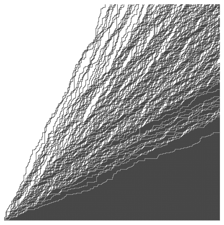
Figure 16. A simulation of the stochastic six vertex model of size $300$ with boundary conditions as in [BCG16] and parameters $\mathsf{L}(0,1;0,1)=0.3$, $\mathsf{L}(1,0;1,0)=0.7$.

Let us briefly discuss two continuous time limits of the stochastic six vertex model. Here we restrict our attention to systems of the type $\mathscr{X}^{\circ}_{{0^{\scriptscriptstyle{M}}};\{v_{t}\}}$, i.e., with a fixed finite number of particles (about other boundary and initial conditions see also §10.1 below). The first of the limits is the well-known ASEP (Asymmetric Simple Exclusion Process) introduced in [Spi70] (see Fig. 17), which is obtained as follows. Observe that for $u=q^{-\frac{1}{2}}+(1-q)q^{-\frac{1}{2}}\epsilon$, we have as $\epsilon\searrow 0$:

$$\mathsf{L}_{u}(0,1;0,1)=\epsilon+O(\epsilon^{2}),\qquad\qquad\mathsf{L}_{u}(1,0;1,0)=q\epsilon+O(\epsilon^{2}).$$

Therefore, for $\epsilon$ small, the particles in the stochastic six vertex model will mostly travel to the right by $1$ at every step. If we subtract this deterministic shift and look at times of order $\epsilon^{-1}$, then the rescaled discrete time process will converge to the continuous time ASEP with $r=1$ and $\ell=q$, see Fig. 18 (note that multiplying both $r$ and $\ell$ by a constant is the same as a deterministic rescaling of the continuous time in the ASEP, and thus is a harmless operation).

Figure 17. The ASEP is a continuous time Markov chain on particle configurations on $\mathbb{Z}$ (in which there is at most one particle per site). Each particle has two exponential clocks of rates $r$ and $\ell$, respectively (all exponential clocks in the process are assumed independent). When the ‘‘$r$’’ clock of a particle rings, it immediately tries to jump to the right by one, and similarly for the ‘‘$\ell$’’ clock and left jumps. If the destination of a jump is already occupied, then the jump is blocked. (This describes the ASEP with finitely many particles, but one can also construct the infinite-particle ASEP following, e.g., the graphical method of [Har78].)

Figure 18. Limit of the six vertex model to the ASEP.

Another continuous time limit is obtained by setting:

$$q=\frac{1-\epsilon}{\alpha},\qquad u=\frac{\epsilon\alpha^{\frac{1}{2}}}{1-\alpha},$$

where $0<\alpha<1$, so that as $\epsilon\to 0$ we have

$$\mathsf{L}_{u}(0,1;0,1)=\alpha+O(\epsilon^{2}),\qquad\qquad\mathsf{L}_{u}(1,0;1,0)=1-\epsilon+O(\epsilon^{2}).$$

At times of order $\epsilon^{-1}$, the system behaves as follows. Each particle at a location $j$ has an exponential clock with rate $1$. When the clock rings, the particle wakes up and performs a jump to the right having the geometric distribution with parameter $\alpha$. However, if in the process of the jump this particle runs into another particle (i.e., its first neighbor on the right), then the moving particle stops at this neighbor’s location, and the neighbor wakes up (and subsequently performs a geometrically distributed jump). See Fig. 19.

Figure 19. A possible jump in the second limit of the stochastic six vertex model. The particle at $x_{k}$ wakes up at rate $1$ and decides to jump by 5 with probability $(1-\alpha)\alpha^{4}$ (waking up means that the particle will jump by at least one). However, $x_{k+1}$ is closer than the intended jump of $x_{k}$, and so $x_{k}$ stops at the location of $x_{k+1}$, and the latter particle wakes up. Then $x_{k+1}$ decides to jump by 4 with probability $(1-\alpha)\alpha^{3}$.

6.6. Degeneration to $q$-Hahn and $q$-Boson systems

In this subsection we will consider another family of degenerations of the higher spin six vertex model which puts no restrictions on the vertical multiplicities. For these degenerations we will need to employ the general $J$ stochastic vertex weights $\mathsf{L}^{{\scriptscriptstyle(J)}}_{u}(i_{1},j_{1};i_{2},j_{2})$ described in §5.2.

Proposition 6.10.

When $u=s$, formula (5.6) for the weights $\mathsf{L}^{{\scriptscriptstyle(J)}}_{u}$ simplifies to the following product form:

$$\mathsf{L}^{{\scriptscriptstyle(J)}}_{s}(i_{1},j_{1};i_{2},j_{2})=\mathbf{1}_{i_{1}+j_{1}=i_{2}+j_{2}}\cdot\mathbf{1}_{j_{2}\leq i_{1}}\cdot(s^{2}q^{J})^{j_{2}}\frac{(q^{-J};q)_{j_{2}}(s^{2}q^{J};q)_{i_{1}-j_{2}}}{(s^{2};q)_{i_{1}}}\frac{(q;q)_{i_{1}}}{(q;q)_{j_{2}}(q;q)_{i_{1}-j_{2}}}.$$ (6.18)

Proof.

To show this, one can directly check that (6.18) satisfies the corresponding recursion relation for $u=s$ (5.5). Alternatively, one can transform the ${}_{4}\bar{\phi}_{3}$ $q$-hypergeometric function to the desired form. We refer to [Bor14, Prop. 6.7] for the complete proof following the second approach. ∎

We see that this degeneration turns the higher spin interacting particle systems described in §6.4 with sequential update into simpler systems with parallel update.

6.6.1. Distribution $\varphi_{q,\upmu,\upnu}$

Before discussing interacting particle systems arising from the vertex weights (6.18), let us focus on the $q$-deformed Beta-binomial distribution appearing in the right-hand side of that formula:

$$\varphi_{q,\upmu,\upnu}(j\,|\,{}m):=\upmu^{j}\frac{(\upnu/\upmu;q)_{j}(\upmu;q)_{m-j}}{(\upnu;q)_{m}}\frac{(q;q)_{m}}{(q;q)_{j}(q;q)_{m-j}},\qquad j\in\{0,1,\ldots,m\}.$$ (6.19)

Here $m\in\mathbb{Z}_{\geq 0}\cup\{+\infty\}$, and the case $m=+\infty$ corresponds to a straightforward limit of (6.19), see (6.23) below. If the parameters belong to one of the following families:

(6.20)

then the weights (6.19) are nonnegative. The above conditions (6.20) replace the nonnegativity conditions (5.1)–(5.2) for this subsection.

We will now discuss several interpretations of the distribution (6.19) which, in particular, will justify its name. The significance of the probability distribution $\varphi_{q,\upmu,\upnu}$ for interacting particle systems was first realized by Povolotsky [Pov13], who showed that it corresponds to the most general ‘‘chipping model’’ (i.e., a particle system as in Fig. 14 with possibly multiple particles leaving a given stack at a time) having parallel update, product-form steady state, and such that the system is solvable by the coordinate Bethe ansatz. He also provided an algebraic interpretation of this distribution:

Proposition 6.11 ([Pov13, Thm. 1]).

Let $A$ and $B$ be two letters satisfying the following quadratic commutation relation:

$$BA=\alpha A^{2}+\beta AB+\gamma B^{2},\qquad\alpha+\beta+\gamma=1.$$

Then

$$\big{(}pA+(1-p)B\big{)}^{m}=\sum_{j=0}^{m}\varphi_{q,\upmu,\upnu}(j\,|\,{}m)A^{j}B^{m-j},$$ (6.21)

where

$$\alpha=\frac{\upnu(1-q)}{1-q\upnu},\qquad\beta=\frac{q-\upnu}{1-q\upnu},\qquad\gamma=\frac{1-q}{1-q\upnu},\qquad\upmu=p+\upnu(1-p).$$

In particular, taking $A=B=1$ in (6.21) implies that the weights (6.19) sum to $1$ over $j=0,1,\ldots,m$. The proof of the above statement is nontrivial, and we will not reproduce it here.

Another interpretation of the $q$-deformed Beta-binomial distribution can be given via a $q$-version of the Pólya’s urn process due to Gnedin and Olshanski [GO09]. Consider the Markov chain on the Pascal triangle

$$\bigsqcup_{m=0}^{\infty}\{(k,\ell)\in\mathbb{Z}^{2}_{\geq 0}\colon k+\ell=m\}$$

with the following transition probabilities (here $m=k+\ell$ is the time in this chain)

Then the distribution of this Markov chain (started from the initial vertex $(0,0)$) at time $m$ is

$$\mathsf{Prob}\big{(}(k,\ell)\big{)}=\varphi_{q,q^{b},q^{a+b}}(k\,|\,{}m),\qquad k=0,1,\ldots,m.$$

More general Markov chains (on the space of interlacing arrays) based on the distributions $\varphi_{q,q^{b},q^{a+b}}$ with negative $a$ and $b$ which have a combinatorial significance (they are $q$-deformations of the classical Robinson–Schensted–Knuth insertion algorithm) were constructed recently in [MP15].

Another feature of the distribution $\varphi_{q,\upmu,\upnu}$ is that it is the weight function for the so-called $q$-Hahn orthogonal polynomials. See [KS96, §3.6] about the polynomials, and [BCPS15a, §5.2] for the exact matching between $\varphi_{q,\upmu,\upnu}$ and the notation related to the $q$-Hahn polynomials.

6.6.2. $q$-Hahn particle system

We will now discuss what the dynamics $\mathscr{X}^{\circ}_{{0^{\scriptscriptstyle{M}}};\{v_{t}\}}$ and $\mathscr{X}^{{\scriptscriptstyle+}}_{\{u_{t}\};{\boldsymbol{\varrho}}}$ look like under the degeneration described in Proposition 6.10. We will first consider the dynamics $\mathscr{X}^{\circ}_{{0^{\scriptscriptstyle{M}}};\{v_{t}\}}$ which lives on particle configurations with a fixed number of particles (say, $M\in\mathbb{Z}_{\geq 0}$), and then will deal with $\mathscr{X}^{{\scriptscriptstyle+}}_{\{u_{t}\};{\boldsymbol{\varrho}}}$. The resulting dynamics will be commonly referred to as the $q$-Hahn particle system with different initial or boundary conditions.

Figure 20. Possible transitions of the $q$-Hahn particle system, with probabilities given on the right (here $\varphi\equiv\varphi_{q,q^{J}s^{2},s^{2}}$). Top: dynamics $\mathscr{X}_{\textnormal{$q$-Hahn}}^{\circ}$ living on configurations with a fixed number of particles. Middle: dynamics $\mathscr{X}_{\textnormal{$q$-Hahn}}^{{\scriptscriptstyle+}}$, in which at each time step $J$ new particles are added at location $1$ ($J=3$ on the picture). Bottom: dynamics $\mathscr{X}_{\textnormal{$q$-Hahn}}^{{\infty}}$ with the initial condition $1^{\infty}2^{0}3^{0}\ldots$.

In order to perform the desired degeneration of $\mathscr{X}^{\circ}$, fix $J\in\mathbb{Z}_{\geq 1}$ and take the time-dependent parameters $\{v_{t}\}$ to be

$$(v_{1},v_{2},\ldots)=(s,qs,\ldots,q^{J-1}s,s,qs,\ldots,q^{J-1}s,\ldots).$$

We will consider the fused dynamics in which one time step corresponds to $J$ steps of the original dynamics. The fused dynamics is Markovian due to the results of §5.2. As follows from §6.4.1, each time step $\mu=0^{m_{0}}1^{m_{1}}2^{m_{2}}\ldots\to\nu=0^{n_{0}}1^{n_{1}}2^{n_{2}}\ldots$ ($\mu,\nu\in\mathsf{Sign}_{M}^{\scriptscriptstyle+}$) of the fused dynamics looks as follows. For each location $x\in\mathbb{Z}_{\geq 0}$, sample $j_{x}\in\{0,1,\ldots,m_{x}\}$ independently of other locations according to the probability distribution $\varphi_{q,q^{J}s^{2},s^{2}}(j_{x}\,|\,{}m_{x})$ (clearly, $j_{x}=m_{x}=0$ for all large enough $x$). Then, in parallel, move $j_{x}$ particles from location $x$ to location $x+1$ for each $x\in\mathbb{Z}_{\geq 0}$, that is, set $n_{x}=m_{x}-j_{x}+j_{x+1}$. Denote this dynamics by $\mathscr{X}_{\textnormal{$q$-Hahn}}^{\circ}$ (see Fig. 20, top).

Note that the weights $\varphi_{q,q^{J}s^{2},s^{2}}$ are nonnegative for $J\in\mathbb{Z}_{\geq 1}$ if $s^{2}\leq 0$ (case 2 in (6.20)), and we are assuming this in our construction.

Remark 6.12.

For $J\in\mathbb{Z}_{\geq 1}$, at most $J$ particles can leave any given location during one time step. However, since the weights of the distribution $\varphi_{q,q^{J}s^{2},s^{2}}$ depend on $q^{J}$ in a rational way, we may analytically continue $\mathscr{X}_{\textnormal{$q$-Hahn}}^{\circ}$ from the case $q^{J}\in q^{\mathbb{Z}_{\geq 1}}$ and $s^{2}\leq 0$, and let the parameters $\upmu=q^{J}\upnu$ and $\upnu=s^{2}$ belong to one of the other families in (6.20). If $\upmu/\upnu\notin q^{\mathbb{Z}_{\geq 1}}$, then an arbitrary number of particles can leave any given location during one time step.

Let us now discuss the degeneration of the dynamics $\mathscr{X}^{{\scriptscriptstyle+}}_{\{u_{t}\};{\boldsymbol{\varrho}}}$. Fix $J\in\mathbb{Z}_{\geq 1}$ and take the time-dependent parameters $\{u_{t}\}$ to be

$$(u_{1},u_{2},\ldots)=(s,qs,\ldots,q^{J-1}s,s,qs,\ldots,q^{J-1}s,\ldots).$$ (6.22)

The corresponding fused dynamics is very similar to $\mathscr{X}_{\textnormal{$q$-Hahn}}^{\circ}$, and the only difference is in the behavior at locations $0$ and $1$. Namely, location $0$ cannot be occupied, and at each time step, exactly $J$ new particles are added at location $1$. Denote this degeneration of $\mathscr{X}^{{\scriptscriptstyle+}}_{\{u_{t}\};{\boldsymbol{\varrho}}}$ by $\mathscr{X}_{\textnormal{$q$-Hahn}}^{{\scriptscriptstyle+}}$ (see Fig. 20, middle).

Because $J\in\mathbb{Z}_{\geq 1}$ particles are added to the configuration at each time step, dynamics $\mathscr{X}_{\textnormal{$q$-Hahn}}^{{\scriptscriptstyle+}}$ cannot be analytically continued in $J$ similarly to Remark 6.12. However, we can simplify this dynamics, by generalizing (6.22) to

$$(u_{1},u_{2},\ldots)=(s,qs,\ldots,q^{K-1}s,s,qs,\ldots,q^{J-1}s,s,qs,\ldots,q^{J-1}s,\ldots),$$

where $K\in\mathbb{Z}_{\geq 1}$ is a new parameter. If we start the corresponding fused dynamics from the empty initial configuration $1^{0}2^{0}\ldots$, then after the first step of this dynamics the configuration will be simply $1^{K}2^{0}3^{0}\ldots$. Moreover, during the evolution, the number of particles at location $1$ will always be $\geq K$. Assume that $|q|<1$, and take $K\to+\infty$. Under the limiting dynamics, at all subsequent times the number of particles leaving location $1$ has the distribution

$$\lim_{i_{1}\to+\infty}\mathsf{L}^{{\scriptscriptstyle(J)}}_{s}(i_{1},j_{1};i_{2},j_{2})=\mathbf{1}_{i_{2}=+\infty}\cdot\varphi_{q,q^{J}s^{2},s^{2}}(j_{2}\,|\,{}{+\infty}),\quad\varphi_{q,\upmu,\upnu}(j\,|\,{}{+\infty})=\upmu^{j}\frac{(\upnu/\upmu;q)_{j}}{(q;q)_{j}}\frac{(\upmu;q)_{\infty}}{(\upnu;q)_{\infty}}.$$ (6.23)

The limit as $K\to+\infty$ clearly does not affect probabilities of particle jumps at all other locations. We will denote the limiting dynamics by $\mathscr{X}_{\textnormal{$q$-Hahn}}^{{\infty}}$ (see Fig. 6.19, bottom). This particle system was introduced in [Pov13]. The system $\mathscr{X}_{\textnormal{$q$-Hahn}}^{{\infty}}$ readily admits an analytic continuation from $q^{J}\in q^{\mathbb{Z}_{\geq 1}}$ and $s^{2}\leq 0$ as in Remark 6.12.

Figure 21. The transition of the $q$-Hahn system $\mathscr{X}_{\textnormal{$q$-Hahn}}^{{\infty}}$ from Fig. 20, bottom, interpreted in terms of the $q$-Hahn TASEP (here $\varphi\equiv\varphi_{q,q^{J}s^{2},s^{2}}$).

Thanks to infinitely many particles at location $1$, the system $\mathscr{X}_{\textnormal{$q$-Hahn}}^{{\infty}}$ admits another nice particle interpretation. Namely, consider right-finite particle configurations $\{x_{1}>x_{2}>x_{3}>\ldots\}$ in $\mathbb{Z}$, in which there can be at most one particle at a given location. For a configuration $\lambda=1^{\infty}2^{\ell_{2}}3^{\ell_{3}}\ldots$ of $\mathscr{X}_{\textnormal{$q$-Hahn}}^{{\infty}}$, let $\ell_{j}=x_{j-1}-x_{j}-1$ (with $x_{0}=+\infty$) be the number of empty spaces between consecutive particles. Let the process start from the step initial configuration $x_{i}(0)=-i$ for all $i$ (corresponding to $\lambda=1^{\infty}2^{0}3^{0}\ldots$). Then during each time step, each particle $x_{i}$ jumps to the right according to the distribution $\varphi_{q,q^{J}s^{2},s^{2}}(\cdot\,|\,{}\mathrm{gap}_{i})$, where $\mathrm{gap}_{i}=\ell_{i}$ is the distance to the nearest right neighbor of $x_{i}$ (the first particle employs the distribution with $\mathrm{gap}_{1}=+\infty$). This system is called the $q$-Hahn TASEP, see Fig. 21. It was introduced in [Pov13], and duality relations for this process were obtained in [Cor14].

Remark 6.13.

In all the above $q$-Hahn systems, one can clearly let the parameter $J$ to depend on time.

6.6.3. $q$-TASEP and $q$-Boson

Let us now perform a further degeneration of the $q$-Hahn TASEP corresponding to the parameters $q$, $\upmu$, and $\upnu$, by setting $\upmu=q\upnu$ (that is, we take $J=1$, and thus must consider $\upnu\leq 0$). Then (6.19) implies that $\varphi_{q,\upmu,\upnu}(j\,|\,{}m)$ vanishes unless $j\leq 1$, and

$$\varphi_{q,\upmu,\upnu}(0\,|\,{}m)=\frac{1-q^{m}\upnu}{1-\upnu},\qquad\qquad \varphi_{q,\upmu,\upnu}(1\,|\,{}m)=\frac{-\upnu(1-q^{m})}{1-\upnu},$$

$$\varphi_{q,\upmu,\upnu}(0\,|\,{}{+\infty})=\frac{1}{1-\upnu},\qquad\qquad \varphi_{q,\upmu,\upnu}(1\,|\,{}{+\infty})=\frac{-\upnu}{1-\upnu}.$$

Taking $\upnu=-\epsilon$ and speeding up the time by $\epsilon^{-1}$, we arrive at the $q$-TASEP — a continuous time particle system on configurations $\{x_{1}>x_{2}>x_{3}>\ldots\}$ on $\mathbb{Z}$ (with no more than one particle per location) in which each particle $x_{i}$ jumps to the right by one at rate $1-q^{\mathrm{gap}_{i}}$, where, as before, $\mathrm{gap}_{i}=x_{i-1}-x_{i}-1$ is the distance to the right neighbor of $x_{i}$.

The $q$-TASEP was introduced in [BC14] (see also [BCS14]), and an ‘‘arrow’’ interpretation of the $q$-TASEP (on configurations $\lambda=1^{\infty}2^{\mathrm{gap}_{2}}3^{\mathrm{gap}_{3}}\ldots$) had been considered much earlier [BBT94], [BIK98], [SW98] under the name of the (stochastic) $q$-Boson system.

It is worth noting that the $q$-Hahn system has a variety of other degenerations, see [Pov13] and [BC15] for examples.

7. Orthogonality relations

In this section we recall two types of (bi)orthogonality relations for the symmetric rational functions $\mathsf{F}_{\lambda}$ (from §4) which first appeared in [BCPS15a]. These relations imply certain Plancherel isomorphism theorems. We also apply biorthogonality to get an integral representation for the functions $\mathsf{G}_{\mu}$. The results of this section provide us with tools which will eventually allow to explicitly evaluate averages of certain observables of the interacting particle systems described in §6 above.

7.1. Spatial biorthogonality

First, we will need the following general statement:

Lemma 7.1.

Let $\{f_{m}(u)\}$, $\{g_{\ell}(u)\}$ be two families of rational functions in $u\in\mathbb{C}$ such that there exist two disjoint finite sets $P_{1},P_{2}\subset\mathbb{C}\cup\{\infty\}$ and positively oriented pairwise nonintersecting closed contours $c_{1},\ldots,c_{k}$ with the following properties:

• All singularities of all the functions $f_{m}(u),g_{\ell}(u)$ lie inside $P_{1}\cup P_{2}$.

• The product $f_{m}(u)g_{\ell}(u)$ does not have singularities in $P_{1}$ if $m<\ell$, and the same product does not have singularities in $P_{2}$ if $m>\ell$.

• For any $i>j$ the contour $c_{i}$ can be shrunk to $P_{1}$ without intersecting the contour $q^{-1}c_{j}$ (equivalently, for any $j<i$ the contour $c_{j}$ can be shrunk to $P_{2}$ without intersecting $q\cdot c_{i}$). Shrinking takes place on the Riemann sphere $\mathbb{C}\cup\{\infty\}$.

Fix $k\in\mathbb{Z}_{\geq 1}$ and two signatures $\mu,\lambda\in\mathsf{Sign}_{k}^{\scriptscriptstyle+}$. If $\mu\neq\lambda$, then for any permutation $\sigma\in\mathfrak{S}_{k}$ we have

$$\oint\limits_{c_{1}}du_{1}\ldots\oint\limits_{c_{k}}du_{k}\prod_{1\leq{\upalpha}<{\upbeta}\leq k}\bigg{(}\frac{u_{\upalpha}-u_{\upbeta}}{u_{\upalpha}-qu_{\upbeta}}\cdot\frac{u_{\sigma({\upalpha})}-qu_{\sigma({\upbeta})}}{u_{\sigma({\upalpha})}-u_{\sigma({\upbeta})}}\bigg{)}\prod_{j=1}^{k}f_{\mu_{j}}(u_{j})g_{\lambda_{\sigma^{-1}(j)}}(u_{j})=0.$$ (7.1)

Proof.

This is a straightforward generalization of Lemma 3.5 in [BCPS15a]. Let us outline the steps of the proof.

We will assume that the integral (7.1) is nonzero, and will show that then it must be that $\lambda=\mu$. First, we observe that, by our assumed structure of the poles,

• If it is possible to shrink the contour $c_{i}$ to $P_{1}$, then for the integral to be nonzero we must have $\mu_{i}\geq\lambda_{\sigma^{-1}(i)}$.

• If it is possible to shrink the contour $c_{i}$ to $P_{2}$, then for the integral to be nonzero we must have $\mu_{i}\leq\lambda_{\sigma^{-1}(i)}$.

Next, using

$$\prod_{1\leq{\upalpha}<{\upbeta}\leq k}\frac{u_{\upalpha}-u_{\upbeta}}{u_{\upalpha}-qu_{\upbeta}}\cdot\frac{u_{\sigma({\upalpha})}-qu_{\sigma({\upbeta})}}{u_{\sigma({\upalpha})}-u_{\sigma({\upbeta})}}=\operatorname{\mathrm{sgn}}(\sigma)\prod_{{\upalpha}<{\upbeta}\colon\sigma({\upalpha})>\sigma({\upbeta})}\frac{u_{\sigma({\upalpha})}-qu_{\sigma({\upbeta})}}{u_{\upalpha}-qu_{\upbeta}}$$ (7.2)

and the properties of the integration contours, we see that

• If for some $i\in\{1,\ldots,k\}$ one has $\sigma(i)>\max(\sigma(1),\ldots,\sigma(i-1))$, then the numerator in the left-hand side of (7.2) contains all terms of the form $(u_{\sigma(i)}-qu_{\sigma(i)+1}),(u_{\sigma(i)}-qu_{\sigma(i)+2}),\ldots,(u_{\sigma(i)}-qu_{k})$, and thus the expression in the right-hand side of (7.2) does not have poles at $u_{\sigma(i)}=qu_{j}$ for all $j>\sigma(i)$. This means that we can shrink the contour $c_{\sigma(i)}$ to $P_{1}$ without picking any residues. This implies that for the integral (7.1) to be nonzero, we must have $\mu_{\sigma(i)}\geq\lambda_{i}$.

• Similarly, if for some $i\in\{1,\ldots,k\}$ one has $\sigma(i)<\min(\sigma(i+1),\ldots,\sigma(k))$, then the contour $c_{\sigma(i)}$ can be shrunk to $P_{2}$, and so the integral (7.1) can be nonzero only if $\mu_{\sigma(i)}\leq\lambda_{i}$.

This completes the argument analogous to Step I of the proof of [BCPS15a, Lemma 3.5]. Further steps of the proof have a purely combinatorial nature and can be repeated without change. We will not reproduce the full combinatorial argument here, but will illustrate it on a concrete example.

Take $\sigma=(3,2,4,5,1,8,6,7)$, and consider an arrow diagram as in Fig. 22. That is, think of the bottom row as $\lambda_{1}\geq\lambda_{2}\geq\ldots\geq\lambda_{8}$ and of the top row as $\mu_{1}\geq\mu_{2}\geq\ldots\geq\mu_{8}$, and draw the corresponding horizontal arrows from larger to smaller integers. Labels in the nodes correspond to the permutation $\sigma$ itself.

Figure 22. Arrow diagram for $\sigma=(3,2,4,5,1,8,6,7)$.

As we read this permutation from left to right, we see running maxima $\sigma(1)$, $\sigma(3)>\max(\sigma(1),\sigma(2))$, $\sigma(4)>\max(\sigma(1),\sigma(2),\sigma(3))$, and $\sigma(6)>\max(\sigma(1),\sigma(2),\sigma(3),\sigma(4),\sigma(5))$, and correspondingly we add (red dashed) arrows $\mu_{\sigma(i)}\to\lambda_{i}$. Similarly, reading the permutation from right to left, we see running minima $\sigma(8)$, $\sigma(7)<\sigma(8)$, and $\sigma(5)<\min(\sigma(6),\sigma(7),\sigma(8))$, and we add (blue solid) arrows $\lambda_{i}\to\mu_{\sigma(i)}$. As one examines the arrow diagram, it becomes obvious that for the integral to be nonzero, we must have

$$\lambda_{1}=\ldots=\lambda_{5}=\mu_{1}=\ldots=\mu_{5},\qquad\lambda_{6}=\lambda_{7}=\lambda_{8}=\mu_{6}=\mu_{7}=\mu_{8}.$$

We also see that any permutation $\sigma$ yielding a nonzero integral (7.1) splits into two blocks permuting $\{1,2,3,4,5\}$ and $\{5,6,7\}$, which are the clusters of equal parts in $\lambda$ and $\mu$. A similar clustering occurs in the general situation, too.

This implies that for the integral (7.1) to be nonzero, we must have $\lambda=\mu$, as desired. ∎

For the orthogonality statements below in this subsection we assume that (5.1) holds.

Definition 7.2.

For any $k\geq 1$, let ${\boldsymbol{\gamma}}^{\scriptscriptstyle+}_{1}[s],\ldots,{\boldsymbol{\gamma}}^{\scriptscriptstyle+}_{k}[s]$ be positively oriented closed contours such that (see Fig. 23)

• Each contour ${\boldsymbol{\gamma}}^{\scriptscriptstyle+}_{{\upalpha}}[s]$ encircles all the points of the set $P_{1}:=\{s\}$, while leaving outside all the points of $P_{2}:=\{s^{-1}\}$.

• For any ${\upbeta}>{\upalpha}$, the interior of ${\boldsymbol{\gamma}}^{\scriptscriptstyle+}_{{\upalpha}}[s]$ contains the contour $q{\boldsymbol{\gamma}}^{\scriptscriptstyle+}_{{\upbeta}}[s]$.

• The contour ${\boldsymbol{\gamma}}^{\scriptscriptstyle+}_{k}[s]$ is sufficiently small so that it does not intersect with $q{\boldsymbol{\gamma}}^{\scriptscriptstyle+}_{k}[s]$.

Also, let ${\boldsymbol{\gamma}}[s;0]$ be a positively oriented closed contour encircling $s,qs,\ldots,q^{k-1}s$, which also contains $q{\boldsymbol{\gamma}}[s;0]$ and leaves $s^{-1}$ outside. Note that $0$ must be inside this contour.

Remark 7.3.

The superscript ‘‘$+$’’ in the contours of Definition 7.2 refers to the property that they are $q$-nested, as opposed to $q^{-1}$-nested contours ${\boldsymbol{\gamma}}^{\scriptscriptstyle-}_{j}[\bullet]$ which we will consider later in §8. Throughout the text points encircled by a contour will be explicitly indicated in the square brackets.

Figure 23. A possible choice of nested integration contours ${\boldsymbol{\gamma}}^{\scriptscriptstyle+}_{i}={\boldsymbol{\gamma}}^{\scriptscriptstyle+}_{i}[s]$, $i=1,2,3$ (Definition 7.2). Contours $q{\boldsymbol{\gamma}}^{\scriptscriptstyle+}_{3}[s]$ and $q^{2}{\boldsymbol{\gamma}}^{\scriptscriptstyle+}_{3}[s]$ are shown dotted. The large contour ${\boldsymbol{\gamma}}[s;0]$ is also shown.

Theorem 7.4.

For any $k\in\mathbb{Z}_{\geq 1}$ and $\lambda,\mu\in\mathsf{Sign}_{k}^{\scriptscriptstyle+}$, we have

$$\oint\limits_{{\boldsymbol{\gamma}}^{\scriptscriptstyle+}_{1}[s]}\frac{du_{1}}{2\pi\mathbf{i}}\ldots\oint\limits_{{\boldsymbol{\gamma}}^{\scriptscriptstyle+}_{k}[s]}\frac{du_{k}}{2\pi\mathbf{i}}\prod_{1\leq{\upalpha}<{\upbeta}\leq k}\frac{u_{\upalpha}-u_{\upbeta}}{u_{\upalpha}-qu_{\upbeta}}\,\mathsf{F}_{\lambda}^{\mathsf{c}}(u_{1},\ldots,u_{k})\prod_{i=1}^{k}\frac{1}{u_{i}-s}\left(\frac{1-su_{i}}{u_{i}-s}\right)^{\mu_{i}}=\mathbf{1}_{\lambda=\mu},$$ (7.3)

where $\mathsf{F}_{\lambda}$ is as in §4.5.

An immediate corollary of Theorem 7.4 is the following ‘‘spatial’’ biorthogonality property of the functions $\mathsf{F}_{\mu}$:

Corollary 7.5.

For any $k\in\mathbb{Z}_{\geq 1}$ and $\lambda,\mu\in\mathsf{Sign}_{k}^{\scriptscriptstyle+}$, we have

$$\frac{\mathsf{c}(\lambda)}{(1-q)^{k}k!}\oint\limits_{{\boldsymbol{\gamma}}[s;0]}\frac{du_{1}}{2\pi\mathbf{i}u_{1}}\ldots\oint\limits_{{\boldsymbol{\gamma}}[s;0]}\frac{du_{k}}{2\pi\mathbf{i}u_{k}}\prod_{1\leq{\upalpha}\neq{\upbeta}\leq k}\frac{u_{\upalpha}-u_{\upbeta}}{u_{\upalpha}-qu_{\upbeta}}\,\mathsf{F}_{\lambda}(u_{1},\ldots,u_{k})\mathsf{F}_{\mu}(u_{1}^{-1},\ldots,u_{k}^{-1})=\mathbf{1}_{\lambda=\mu},$$ (7.4)

with $\mathsf{c}(\cdot)$ as in (4.12).

We call this property spatial biorthogonality because for, say, fixed $\lambda$ and varying $\mu$, the right-hand side is the delta function in the spatial variables $\mu$. This should be compared to the spectral biorthogonality of Theorem 7.10 with delta functions in spectral variables in the right-hand side.

Theorem 7.4 and Corollary 7.5 were conjectured in [Pov13] and proved in [BCPS15a, §3] (see also [Bor14, Thm. 7.2]). Here we present an outline of the proof in which the abstract combinatorial part (Lemma 7.1) is separated from a concrete form of integration contours. This makes the proof applicable in more general situations which will be discussed in a subsequent publication.

Proof of Corollary 7.5.

Assuming Theorem 7.4, deform the integration contours ${\boldsymbol{\gamma}}^{\scriptscriptstyle+}_{1}[s],\ldots,{\boldsymbol{\gamma}}^{\scriptscriptstyle+}_{k}[s]$ (in this order) to ${\boldsymbol{\gamma}}[s;0]$. One readily sees that this does not lead to any additional residues. Next, observe that the integral over all $u_{j}\in{\boldsymbol{\gamma}}[s;0]$ is invariant under permutations of the $u_{j}$’s, and thus one can perform the symmetrization and divide by $k!$. This leads to

$$\mathbf{1}_{\lambda=\mu}=\frac{(1-q)^{-k}}{k!}\oint\limits_{{\boldsymbol{\gamma}}[s;0]}\frac{du_{1}}{2\pi\mathbf{i}u_{1}}\ldots\oint\limits_{{\boldsymbol{\gamma}}[s;0]}\frac{du_{k}}{2\pi\mathbf{i}u_{k}}\prod_{1\leq{\upalpha}\neq{\upbeta}\leq k}\frac{u_{\upalpha}-u_{\upbeta}}{u_{\upalpha}-qu_{\upbeta}}\mathsf{F}_{\lambda}^{\mathsf{c}}(u_{1},\ldots,u_{k})\\ \times\underbrace{\sum_{\sigma\in\mathfrak{S}_{k}}\prod_{1\leq{\upbeta}<{\upalpha}\leq k}\frac{u_{\sigma({\upalpha})}-qu_{\sigma({\upbeta})}}{u_{\sigma({\upalpha})}-u_{\sigma({\upbeta})}}\prod_{i=1}^{k}\frac{1-q}{1-su_{\sigma(i)}^{-1}}\bigg{(}\frac{1-su_{\sigma(i)}}{u_{\sigma(i)}-s}\bigg{)}^{\mu_{i}}}_{\textnormal{$\mathsf{F}_{\mu}(u_{1}^{-1},\ldots,u_{k}^{-1})$ by \eqref{F_symm_formula}}},$$

as desired. ∎

Proof of Theorem 7.4.

Fix $k$ and signatures $\lambda$ and $\mu$. In order to apply Lemma 7.1, set

$$f_{m}(u):=\frac{1-q}{u-s}\left(\frac{1-su}{u-s}\right)^{m},\qquad g_{\ell}(u):=\frac{1-q}{1-su}\left(\frac{u-s}{1-su}\right)^{\ell},$$

and use $P_{1}=\{s\}$ and $P_{2}=\{s^{-1}\}$. If $m>\ell$, then all singularities of $f_{m}(u)g_{\ell}(u)$ are in $P_{1}$, and if $m<\ell$, then all singularities of this product are in $P_{2}$. By virtue of the symmetrization formula for $\mathsf{F}_{\lambda}$ (4.24), we see that the integrand in (7.3) is (up to a multiplicative constant) the same as the one in Lemma 7.1 (with the above specialization of $f_{m}$ and $g_{\ell}$). The structure of our integration contours ${\boldsymbol{\gamma}}^{\scriptscriptstyle+}_{j}[s]$ and the fact that $\infty\notin P_{1}\cup P_{2}$ (so the contours can be dragged through infinity without picking the residues) implies that the third condition of Lemma 7.1 is also satisfied. Thus, we conclude that the integral in (7.3) vanishes unless $\mu=\lambda$.

Example.

To better illustrate the application of Lemma 7.1 here, consider contours ${\boldsymbol{\gamma}}^{\scriptscriptstyle+}_{1}[s],{\boldsymbol{\gamma}}^{\scriptscriptstyle+}_{2}[s]$, and ${\boldsymbol{\gamma}}^{\scriptscriptstyle+}_{3}[s]$ as in Fig. 23. Depending on $\sigma$, the denominator in the integrand in (7.1) contains some of the factors $u_{1}-qu_{2}$, $u_{1}-qu_{3}$, and $u_{2}-qu_{3}$. The contour ${\boldsymbol{\gamma}}^{\scriptscriptstyle+}_{3}[s]$ can always be shrunk to $P_{1}$ without picking residues at $u_{3}=q^{-1}u_{1}$ and $u_{3}=q^{-1}u_{2}$ (this is the assumption on the contours in Lemma 7.1). Moreover, if, for example, the permutation $\sigma$ provides a cancellation of the factor $u_{2}-qu_{3}$ in the denominator, then the contour ${\boldsymbol{\gamma}}^{\scriptscriptstyle+}_{2}[s]$ can also be shrunk to $P_{1}$ without picking the residue at $u_{2}=qu_{3}$. Similarly, the contour ${\boldsymbol{\gamma}}^{\scriptscriptstyle+}_{1}[s]$ can always be expanded (‘‘shrunk’’ on the Riemann sphere) to $P_{2}$ (recall that infinity does not supply any residues), and if the factor $u_{1}-qu_{2}$ in the denominator is canceled for a certain $\sigma$, then ${\boldsymbol{\gamma}}^{\scriptscriptstyle+}_{2}[s]$ can also be expanded to $P_{2}$ without picking the residue at $u_{2}=q^{-1}u_{1}$.

Now we must consider the case when $\mu=\lambda$, that is, evaluate the ‘‘squared norm’’ of $\mathsf{F}_{\mu}$. Arguing similarly to the example in the proof of Lemma 7.1 (see [BCPS15a, Lemma 3.5] for more detail), we see that the integral

$$\sum_{\sigma\in\mathfrak{S}_{k}}\oint\limits_{{\boldsymbol{\gamma}}^{\scriptscriptstyle+}_{1}[s]}\frac{du_{1}}{2\pi\mathbf{i}}\ldots\oint\limits_{{\boldsymbol{\gamma}}^{\scriptscriptstyle+}_{k}[s]}\frac{du_{k}}{2\pi\mathbf{i}}\prod_{1\leq{\upalpha}<{\upbeta}\leq k}\bigg{(}\frac{u_{\upalpha}-u_{\upbeta}}{u_{\upalpha}-qu_{\upbeta}}\frac{u_{\sigma({\upalpha})}-qu_{\sigma({\upbeta})}}{u_{\sigma({\upalpha})}-u_{\sigma({\upbeta})}}\bigg{)}\prod_{i=1}^{k}\frac{1}{(u_{i}-s)(1-su_{i})}\left(\frac{u_{i}-s}{1-su_{i}}\right)^{\lambda_{\sigma^{-1}(i)}-\lambda_{i}}$$ (7.5)

(this is the same as the left-hand side of (7.3) with $\mu=\lambda$, up to the constant $(1-q)^{k}\mathsf{c}(\lambda)$) vanishes unless $\sigma\in\mathfrak{S}_{k}$ permutes within clusters of the signature $\lambda$, that is, $\sigma$ must preserve each maximal set of indices $\{a,a+1,\ldots,b\}\subseteq\{1,\ldots,k\}$ for which $\lambda_{a}=\lambda_{a+1}=\ldots=\lambda_{b}$. Let $c_{\lambda}$ be the number of such clusters in $\lambda$. Denote the set of all permutations permuting within clusters of $\lambda$ by $\mathfrak{S}_{k}^{(\lambda)}$. Any permutation $\sigma\in\mathfrak{S}_{k}^{(\lambda)}$ can be represented as a product of $c_{\lambda}$ permutations $\sigma_{1},\ldots,\sigma_{c_{\lambda}}$, with each $\sigma_{i}$ fixing all elements of $\{1,\ldots,k\}$ except those belonging to the $i$-th cluster of $\lambda$. We will denote the set of indices within the $i$-th cluster by $C_{i}(\lambda)$, and write $\sigma_{i}\in\mathfrak{S}_{k}^{(\lambda,i)}$. For example, if $k=5$ and $\lambda_{1}=\lambda_{2}=\lambda_{3}>\lambda_{4}=\lambda_{5}$, then $c_{\lambda}=2$, and the permutation $\sigma\in\mathfrak{S}_{k}^{(\lambda)}$ must stabilize the sets $C_{1}(\lambda)=\{1,2,3\}$ and $C_{2}(\lambda)=\{4,5\}$; $\mathfrak{S}_{k}^{(\lambda,1)}$ is the set of all permutations of $\{1,2,3\}$, and $\mathfrak{S}_{k}^{(\lambda,2)}$ is the set of all permutations of $\{4,5\}$.

Therefore, the sum in (7.5) is only over $\sigma\in\mathfrak{S}_{k}^{(\lambda)}$. Let us now compute it. We have

$$\sum_{\sigma\in\mathfrak{S}_{k}^{(\lambda)}}\prod_{1\leq{\upalpha}<{\upbeta}\leq k}\frac{u_{\sigma({\upalpha})}-qu_{\sigma({\upbeta})}}{u_{\sigma({\upalpha})}-u_{\sigma({\upbeta})}}\prod_{i=1}^{k}\frac{1}{(u_{i}-s)(1-su_{i})}\left(\frac{u_{i}-s}{1-su_{i}}\right)^{\lambda_{\sigma^{-1}(i)}-\lambda_{i}}\\ =\prod_{r=1}^{k}\frac{1}{(u_{r}-s)(1-su_{r})}\cdot\prod_{1\leq i<j\leq c_{\lambda}}\prod_{\begin{subarray}{c}{\upalpha}\in C_{i}(\lambda)\\ {\upbeta}\in C_{j}(\lambda)\end{subarray}}\frac{u_{\upalpha}-qu_{\upbeta}}{u_{\upalpha}-u_{\upbeta}}\cdot\prod_{i=1}^{c_{\lambda}}\sum_{\sigma_{i}\in\mathfrak{S}_{k}^{(\lambda,i)}}\prod_{\begin{subarray}{c}1\leq{\upalpha}<{\upbeta}\leq k\\ {\upalpha},{\upbeta}\in C_{i}(\lambda)\end{subarray}}\frac{u_{\sigma_{i}({\upalpha})}-qu_{\sigma_{i}({\upbeta})}}{u_{\sigma_{i}({\upalpha})}-u_{\sigma_{i}({\upbeta})}}.$$

For each sum over $\sigma_{i}\in\mathfrak{S}_{k}^{(\lambda,i)}$ we can use the symmetrization identity (footnote${}^{\ref{symm_footnote}}$). Thus, (7.5) becomes

$$\sum_{\sigma\in\mathfrak{S}_{k}}\oint\limits_{{\boldsymbol{\gamma}}^{\scriptscriptstyle+}_{1}[s]}\frac{du_{1}}{2\pi\mathbf{i}}\ldots\oint\limits_{{\boldsymbol{\gamma}}^{\scriptscriptstyle+}_{k}[s]}\frac{du_{k}}{2\pi\mathbf{i}}\prod_{{\upalpha}<{\upbeta}}\bigg{(}\frac{u_{\upalpha}-u_{\upbeta}}{u_{\upalpha}-qu_{\upbeta}}\frac{u_{\sigma({\upalpha})}-qu_{\sigma({\upbeta})}}{u_{\sigma({\upalpha})}-u_{\sigma({\upbeta})}}\bigg{)}\prod_{i=1}^{k}\frac{1}{(u_{i}-s)(1-su_{i})}\left(\frac{u_{i}-s}{1-su_{i}}\right)^{\lambda_{\sigma^{-1}(i)}-\lambda_{i}}\\ =(1-q)^{-k}\prod_{i\geq 0}(q;q)_{\ell_{i}}\oint\limits_{{\boldsymbol{\gamma}}^{\scriptscriptstyle+}_{1}[s]}\frac{du_{1}}{2\pi\mathbf{i}}\ldots\oint\limits_{{\boldsymbol{\gamma}}^{\scriptscriptstyle+}_{k}[s]}\frac{du_{k}}{2\pi\mathbf{i}}\prod_{i=1}^{c_{\lambda}}\prod_{\begin{subarray}{c}1\leq{\upalpha}<{\upbeta}\leq k\\ {\upalpha},{\upbeta}\in C_{i}(\lambda)\end{subarray}}\frac{u_{\upalpha}-u_{\upbeta}}{u_{\upalpha}-qu_{\upbeta}}\prod_{r=1}^{k}\frac{1}{(u_{r}-s)(1-su_{r})},$$

where we have used the usual multiplicative notation $\lambda=0^{\ell_{0}}1^{\ell_{1}}2^{\ell_{2}}\ldots$. The integration variables above corresponding to each cluster are now independent, and thus the integral reduces to a product of $c_{\lambda}$ smaller nested contour integrals of similar form. Each of these smaller integrals can be computed as follows:

$$\oint\limits_{{\boldsymbol{\gamma}}^{\scriptscriptstyle+}_{1}[s]}\frac{du_{1}}{2\pi\mathbf{i}}\oint\limits_{{\boldsymbol{\gamma}}^{\scriptscriptstyle+}_{2}[s]}\frac{du_{2}}{2\pi\mathbf{i}}\ldots\oint\limits_{{\boldsymbol{\gamma}}^{\scriptscriptstyle+}_{\ell}[s]}\frac{du_{\ell}}{2\pi\mathbf{i}}\prod_{1\leq{\upalpha}<{\upbeta}\leq\ell}\frac{u_{\upalpha}-u_{\upbeta}}{u_{\upalpha}-qu_{\upbeta}}\prod_{i=1}^{\ell}\frac{1}{(u_{i}-s)(1-su_{i})}$$

$$\hskip 40.0pt=\frac{1}{1-s^{2}}\oint\limits_{{\boldsymbol{\gamma}}^{\scriptscriptstyle+}_{2}[s]}\frac{du_{2}}{2\pi\mathbf{i}}\ldots\oint\limits_{{\boldsymbol{\gamma}}^{\scriptscriptstyle+}_{\ell}[s]}\frac{du_{\ell}}{2\pi\mathbf{i}}\prod_{j=2}^{\ell}\frac{1-su_{j}}{1-qsu_{j}}\prod_{2\leq{\upalpha}<{\upbeta}\leq\ell}\frac{u_{\upalpha}-u_{\upbeta}}{u_{\upalpha}-qu_{\upbeta}}\prod_{i=2}^{\ell}\frac{1}{(u_{i}-s)(1-su_{i})}$$

$$\hskip 40.0pt=\frac{1}{1-s^{2}}\oint\limits_{{\boldsymbol{\gamma}}^{\scriptscriptstyle+}_{2}[s]}\frac{du_{2}}{2\pi\mathbf{i}}\ldots\oint\limits_{{\boldsymbol{\gamma}}^{\scriptscriptstyle+}_{\ell}[s]}\frac{du_{\ell}}{2\pi\mathbf{i}}\prod_{2\leq{\upalpha}<{\upbeta}\leq\ell}\frac{u_{\upalpha}-u_{\upbeta}}{u_{\upalpha}-qu_{\upbeta}}\prod_{i=2}^{\ell}\frac{1}{(u_{i}-s)(1-qsu_{i})}$$

$$\hskip 40.0pt=\textnormal{etc.}$$

$$\hskip 40.0pt=\frac{1}{(s^{2};q)_{\ell}}.$$

Indeed, there is only one $u_{1}$-pole outside the contour ${\boldsymbol{\gamma}}^{\scriptscriptstyle+}_{1}[s]$, namely, $u_{1}=s^{-1}$. Evaluating the integral over $u_{1}$ by taking the minus residue at $u_{1}=s^{-1}$ leads to a smaller similar integral with the outside pole $s^{-1}$ replaced by $(qs)^{-1}$. Continuing in the same way with integration over $u_{2},\ldots,u_{\ell}$, we obtain ${1}/{(s^{2};q)_{\ell}}$. Putting together all of the above components, we see that we have established the desired claim. ∎

7.2. Plancherel isomorphisms and completeness

Here we discuss Plancherel isomorphism results related to the functions $\mathsf{F}_{\lambda}$. This subsection is essentially a citation from [BCPS15a] and [Bor14].

Let us fix the number of variables $n\in\mathbb{Z}_{\geq 1}$ and assume (5.1), as usual. Extend the definition of the functions $\mathsf{F}_{\lambda}(u_{1},\ldots,u_{n})$ to all $\lambda\in\mathsf{Sign}_{n}$ using the same symmetrization formula (4.24). These functions also satisfy the shifting property (4.26).

Definition 7.6 (Function spaces).

Denote the space of functions $f(\lambda)$ on $\mathsf{Sign}_{n}$ with finite support by $\mathcal{W}^{n}$. Also, denote by $\mathcal{C}^{n}$ the space of symmetric Laurent polynomials $R(u_{1},\ldots,u_{n})$ in the variables $\frac{u_{i}-s}{1-su_{i}}$, $i=1,\ldots,n$, with the additional requirement that $R(u_{1},\ldots,u_{n})$ converges to zero as $|u_{i}|\to\infty$ for any $i$.

Note that as functions in $\lambda$, the $\mathsf{F}_{\lambda}(u_{1},\ldots,u_{n})$’s clearly do not belong to $\mathcal{W}^{n}$. However, as functions in the $u_{i}$’s, they belong to $\mathcal{C}^{n}$, because we can use

$$\frac{1}{1-su}=\frac{1}{1-s^{2}}+\frac{s}{1-s^{2}}\frac{u-s}{1-su}$$

to rewrite the prefactor in (4.24) containing $\prod_{i=1}^{n}(1-su_{i})^{-1}$ as a Laurent polynomial in the desired variables. (A Laurent polynomial in $\frac{u_{i}-s}{1-su_{i}}$ is clearly bounded at infinity, and this simple computation shows that it can decay, too.) The sum over $\sigma$ readily produces a symmetric Laurent polynomial in $\frac{u_{i}-s}{1-su_{i}}$ because all the factors in the denominator of the form $u_{\upalpha}-u_{\upbeta}$ cancel out. Finally, $\mathsf{F}_{\lambda}(u_{1},\ldots,u_{n})$ clearly goes to zero as $|u_{i}|\to\infty$.

Definition 7.7 (Plancherel transforms).

The direct transform $\mathscr{F}$ maps a function $f$ from $\mathcal{W}^{n}$ to $\mathscr{F}f\in\mathcal{C}^{n}$ and acts as

$$(\mathscr{F}f)(u_{1},\ldots,u_{n}):=\sum_{\lambda\in\mathsf{Sign}_{n}}f(\lambda)\mathsf{F}_{\lambda}(u_{1},\ldots,u_{n}).$$

The inverse transform $\mathscr{J}$ takes $R\in\mathcal{C}^{n}$ to $\mathscr{J}R\in\mathcal{W}^{n}$ and acts as

$$(\mathscr{J}R)(\lambda):=\mathsf{c}(\lambda)\oint\limits_{{\boldsymbol{\gamma}}^{\scriptscriptstyle+}_{1}[s]}\frac{du_{1}}{2\pi\mathbf{i}}\ldots\oint\limits_{{\boldsymbol{\gamma}}^{\scriptscriptstyle+}_{n}[s]}\frac{du_{n}}{2\pi\mathbf{i}}\prod_{1\leq{\upalpha}<{\upbeta}\leq n}\frac{u_{\upalpha}-u_{\upbeta}}{u_{\upalpha}-qu_{\upbeta}}R(u_{1},\ldots,u_{n})\prod_{i=1}^{n}\frac{1}{u_{i}-s}\left(\frac{1-su_{i}}{u_{i}-s}\right)^{\lambda_{i}},$$

where $\mathsf{c}(\lambda)$ is defined by (4.12). Let us explain why $\mathscr{J}R$ has finite support in $\lambda$. If $\lambda_{1}\geq M$ for sufficiently large $M>0$, then the integrand has no pole at $s^{-1}$ outside ${\boldsymbol{\gamma}}^{\scriptscriptstyle+}_{1}[s]$, and thus vanishes. (It is crucial that $R$ vanishes at $u_{1}=\infty$, so that the integrand has no residue at $u_{1}=\infty$.) Similarly, if $\lambda_{n}\leq-M$, then there is no $u_{n}$-pole at $s$ inside ${\boldsymbol{\gamma}}^{\scriptscriptstyle+}_{n}[s]$, and so the integral also vanishes. Clearly, the bound $M$ depends on the function $R$.

Remark 7.8.

Similarly to [BCPS15a, Proposition 3.2], the nested contours in the transform $\mathscr{J}$ can be replaced by two different families of identical contours, which allows to symmetrize under the integral and interpret $\mathscr{J}R$ as a bilinear pairing between $R$ and $\mathsf{F}^{\mathsf{c}}_{\lambda}(u_{1}^{-1},\ldots,u_{n}^{-1})$. One of the choices of these identical contours is ${\boldsymbol{\gamma}}[s;0]$, cf. Corollary 7.5. Another one is the small contour ${\boldsymbol{\gamma}}^{\scriptscriptstyle+}_{1}[s]$ around $s$, but the formula for $\mathscr{J}$ would then involve string specializations of the $u_{i}$’s. We refer to [BCPS15b] and [BCPS15a] for details.

Theorem 7.9 (Plancherel isomorphisms [BCPS15a, Theorems 3.4 and 3.9]).

The operator $f\mapsto\mathscr{J}(\mathscr{F}f)$ acts as the identity on $\mathcal{W}^{n}$. The operator $R\mapsto\mathscr{F}(\mathscr{J}R)$ acts as the identity on $\mathcal{C}^{n}$.

The first statement is clearly equivalent to Theorem 7.4 established above (note that by (4.26), identities (7.3) and (7.4) are invariant under simultaneous shifts in $\lambda$ and $\mu$, and thus also hold for all $\lambda,\mu\in\mathsf{Sign}_{n}$). The second statement follows from the spectral biorthogonality which can be established independently:

Theorem 7.10.

The functions $\mathsf{F}_{\lambda}$ satisfy the spectral biorthogonality relation

$$\sum_{\lambda\in\mathsf{Sign}_{n}}\mathop{\oint\ldots\oint}\frac{d\mathbf{u}}{(2\pi\mathbf{i})^{n}}\mathop{\oint\ldots\oint}\frac{d\mathbf{v}}{(2\pi\mathbf{i})^{n}}\phi(\mathbf{u})\psi(\mathbf{v})\mathsf{F}_{\lambda}(\mathbf{u})\mathsf{F}^{\mathsf{c}}_{\lambda}(\bar{\mathbf{v}})\prod_{1\leq{\upalpha}<{\upbeta}\leq n}(u_{{\upalpha}}-u_{{\upbeta}})(v_{{\upalpha}}-v_{{\upbeta}})\\ =(-1)^{\frac{n(n-1)}{2}}\mathop{\oint\ldots\oint}\frac{d\mathbf{u}}{(2\pi\mathbf{i})^{n}}\prod_{1\leq{\upalpha},{\upbeta}\leq n}(u_{{\upalpha}}-qu_{{\upbeta}})\cdot\phi(\mathbf{u})\sum_{\sigma\in\mathfrak{S}_{n}}\operatorname{\mathrm{sgn}}(\sigma)\psi(\sigma\mathbf{u}),$$

where $\phi$ and $\psi$ are test functions, and each integration above is performed over one and the same sufficiently small contour encircling $s$ while leaving $s^{-1}$ outside.

Informally, the spectral biorthogonality can be written as

$$\prod_{1\leq{\upalpha}<{\upbeta}\leq n}(u_{{\upalpha}}-u_{{\upbeta}})(v_{{\upalpha}}-v_{{\upbeta}})\sum_{\lambda\in\mathsf{Sign}_{n}}\mathsf{F}_{\lambda}(\mathbf{u})\mathsf{F}^{\mathsf{c}}_{\lambda}(\bar{\mathbf{v}})=(-1)^{\frac{n(n-1)}{2}}\prod_{1\leq{\upalpha},{\upbeta}\leq n}(u_{{\upalpha}}-qu_{{\upbeta}})\cdot\det[\delta(v_{i}-u_{j})]_{i,j=1}^{n}.$$

Two different ways of making Theorem 7.10 precise (by choosing suitable classes of test functions $\phi$ and $\psi$) are presented in [BCPS15a, §4] and [Bor14, §7], along with two corresponding proofs. These proofs differ significantly, and the proof in [Bor14] directly utilizes the Cauchy identity (Proposition 4.11).

Example ($n=1$).

Let us illustrate the connections between spatial and spectral biorthogonality statements and the Cauchy identity in the simplest one-variable case. For that, let us consider the following variant of the Cauchy identity:

$$\sum_{n=0}^{\infty}\frac{z^{n}}{w^{n+1}}=\frac{1}{w-z},\qquad\left|\frac{z}{w}\right|<1.$$

By shifting the summation index towards $-\infty$, we can write

$$\sum_{n=-M}^{\infty}\frac{z^{n}}{w^{n+1}}=\frac{w^{M}}{z^{M}}\frac{1}{w-z},\qquad\left|\frac{z}{w}\right|<1.$$

Now take contour integrals in $z$ and $w$ (over positively oriented circles with $|z|<|w|$) of both sides of this relation multiplied by $P(z)Q(w)$, where $P$ and $Q$ are Laurent polynomials. Then in the left-hand side we obtain the same sum for any $M\gg 1$, and in the right-hand side the $w$ contour can be shrunk to zero, thus picking the residue at $w=z$. Therefore, we have

$$\sum_{n=-\infty}^{\infty}\oint\oint\frac{z^{n}}{w^{n+1}}\,P(z)Q(w)\frac{dz}{2\pi\mathbf{i}}\frac{dw}{2\pi\mathbf{i}}=\oint P(z)Q(z)\frac{dz}{2\pi\mathbf{i}}.$$

The convergence condition $|z|<|w|$ is irrelevant for the left-hand side because the sum over $n$ now contains only finitely many terms. The resulting spectral biorthogonality can be informally written as

$$\sum_{n=-\infty}^{\infty}\frac{z^{n}}{w^{n+1}}=\delta(w-z).$$

To get the other biorthogonality relation, integrate both sides of the above identity against $w^{m}\frac{dw}{2\pi\mathbf{i}}$, $m\in\mathbb{Z}$. Since $\{z^{n}\}_{n\in\mathbb{Z}}$ are linearly independent, we obtain

$$\oint_{|w|=\textnormal{const}}w^{m}\frac{1}{w^{n+1}}\frac{dw}{2\pi\mathbf{i}}=\mathbf{1}_{m=n}.$$

This is the spatial biorthogonality relation. This identity also readily follows from the Cauchy’s integral formula.

Similar considerations work for Cauchy identities in several variables. The second type of biorthogonality relations can often be verified independently in a simpler fashion (as in the proof of Theorem 7.4).

Plancherel isomorphism results (Theorem 7.9) imply that the (coordinate) Bethe ansatz yielding the eigenfunctions $\mathsf{F}_{\lambda}$ of the transfer matrices is complete. That is, any function $f\in\mathcal{W}^{n}$ can be mapped into the spectral space, and then reconstructed back from its image. One of the ways to write down this completeness statement (using the orthogonality relation (7.4)) is the following:

$$f(\lambda)=\frac{1}{(1-q)^{n}n!}\oint\limits_{{\boldsymbol{\gamma}}[s;0]}\frac{du_{1}}{2\pi\mathbf{i}u_{1}}\ldots\oint\limits_{{\boldsymbol{\gamma}}[s;0]}\frac{du_{n}}{2\pi\mathbf{i}u_{n}}\prod_{1\leq{\upalpha}\neq{\upbeta}\leq n}\frac{u_{\upalpha}-u_{\upbeta}}{u_{\upalpha}-qu_{\upbeta}}\,(\mathscr{F}f)(u_{1},\ldots,u_{n})\mathsf{F}^{\mathsf{c}}_{\lambda}(u_{1}^{-1},\ldots,u_{n}^{-1}).$$

Remark 7.11 (Spectral decomposition of $\mathscr{Q}^{\circ}_{{0^{\scriptscriptstyle{m}}};v}$).

Relation (7.4) also implies a spectral decomposition of the operator $\mathscr{Q}^{\circ}_{{0^{\scriptscriptstyle{m}}};v}$ acting on functions on $\mathsf{Sign}_{m}^{\scriptscriptstyle+}$, cf. Remark 6.6:

$$\mathscr{Q}^{\circ}_{{0^{\scriptscriptstyle{m}}};v}(\mu\to\nu)=\frac{(-s)^{|\nu|-|\mu|}}{(1-q)^{m}m!}\oint\limits_{{\boldsymbol{\gamma}}[s;0]}\frac{dz_{1}}{2\pi\mathbf{i}z_{1}}\ldots\oint\limits_{{\boldsymbol{\gamma}}[s;0]}\frac{dz_{m}}{2\pi\mathbf{i}z_{m}}\prod_{1\leq{\upalpha}\neq{\upbeta}\leq m}\frac{z_{\upalpha}-z_{\upbeta}}{z_{\upalpha}-qz_{\upbeta}}\\ \times\bigg{(}\prod_{i=1}^{m}\frac{1-qz_{i}v}{1-z_{i}v}\bigg{)}\mathsf{F}_{\mu}(z_{1},\ldots,z_{m})\mathsf{F}_{\nu}^{\mathsf{c}}(z_{1}^{-1},\ldots,z_{m}^{-1}).$$ (7.6)

Indeed, by (6.12) this operator has eigenfunctions $\Psi_{\lambda}(z_{1},\ldots,z_{m})=(-s)^{-|\lambda|}\mathsf{F}_{\lambda}(z_{1},\ldots,z_{m})$ with eigenvalues $\displaystyle\prod\nolimits_{i=1}^{m}\frac{1-qz_{i}v}{1-z_{i}v}$ (the constant $(q;q)_{m}$ can be ignored). Thus, (7.6) follows by multiplying the eigenrelation (6.12) by $(-s)^{|\nu|}\mathsf{F}^{\mathsf{c}}_{\nu}(z_{1}^{-1},\ldots,z_{m}^{-1})$ and integrating as in (7.4). Since the identity (6.12) requires the admissibility $({z_{i}},{v})\in\mathsf{Adm}$ (Definition 4.7) before the integration, in (7.6) the point $v^{-1}$ should be outside the integration contour ${\boldsymbol{\gamma}}[s;0]$ (the argument for this is similar to the proof of Proposition 7.13 below).

Remark 7.12.

Function spaces $\mathcal{W}^{n}$ and $\mathcal{C}^{n}$ are far from being optimal. This is because we only address algebraic aspects of Plancherel isomorphisms. An extension of the first Plancherel isomorphism to larger spaces is described in [CP16, Appendix A].

7.3. An integral representation for $\mathsf{G}_{\mu}$

Using the orthogonality result of Theorem 7.4 and the Cauchy identity, we can obtain relatively simple nested contour integral formulas for the skew functions $\mathsf{G}_{\mu/\kappa}$ (and, in particular, for $\mathsf{G}_{\mu}$), which will be useful later in §8 and §9.

Proposition 7.13.

For any $k,N\in\mathbb{Z}_{\geq 1}$, $\mu,\kappa\in\mathsf{Sign}_{k}^{\scriptscriptstyle+}$, and $v_{1},\ldots,v_{N}$ such that the $v_{i}^{-1}$’s are outside of all the integration contours ${\boldsymbol{\gamma}}^{\scriptscriptstyle+}_{j}[s]$ of Definition 7.2, we have

$$\mathsf{G}_{\mu/\kappa}(v_{1},\ldots,v_{N})=\oint\limits_{{\boldsymbol{\gamma}}^{\scriptscriptstyle+}_{1}[s]}\frac{du_{1}}{2\pi\mathbf{i}}\ldots\oint\limits_{{\boldsymbol{\gamma}}^{\scriptscriptstyle+}_{k}[s]}\frac{du_{k}}{2\pi\mathbf{i}}\prod_{1\leq{\upalpha}<{\upbeta}\leq k}\frac{u_{\upalpha}-u_{\upbeta}}{u_{\upalpha}-qu_{\upbeta}}\\ \times\mathsf{F}_{\kappa}^{\mathsf{c}}(u_{1},\ldots,u_{k})\prod_{i=1}^{k}\frac{1}{u_{i}-s}\left(\frac{1-su_{i}}{u_{i}-s}\right)^{\mu_{i}}\prod_{\begin{subarray}{c}1\leq i\leq k\\ 1\leq j\leq N\end{subarray}}\frac{1-qu_{i}v_{j}}{1-u_{i}v_{j}}.$$ (7.7)

When $\kappa=(0^{k})$, with the help of (4.22), formula (4.18) reduces to

Corollary 7.14 ([Bor14, Prop. 7.3]).

Under the assumptions of Proposition 7.13 above,

$$\mathsf{G}_{\mu}(v_{1},\ldots,v_{N})=(s^{2};q)_{k}\oint\limits_{{\boldsymbol{\gamma}}^{\scriptscriptstyle+}_{1}[s]}\frac{du_{1}}{2\pi\mathbf{i}}\ldots\oint\limits_{{\boldsymbol{\gamma}}^{\scriptscriptstyle+}_{k}[s]}\frac{du_{k}}{2\pi\mathbf{i}}\prod_{1\leq{\upalpha}<{\upbeta}\leq k}\frac{u_{\upalpha}-u_{\upbeta}}{u_{\upalpha}-qu_{\upbeta}}\\ \times\prod_{i=1}^{k}\frac{1}{(u_{i}-s)(1-su_{i})}\left(\frac{1-su_{i}}{u_{i}-s}\right)^{\mu_{i}}\prod_{\begin{subarray}{c}1\leq i\leq k\\ 1\leq j\leq N\end{subarray}}\frac{1-qu_{i}v_{j}}{1-u_{i}v_{j}}.$$ (7.8)

Proof of Proposition 7.13.

Fix $\mu,\kappa\in\mathsf{Sign}_{k}^{\scriptscriptstyle+}$, multiply both sides of (7.3) by $\mathsf{G}_{\lambda/\kappa}(v_{1},\ldots,v_{N})$, and sum over $\lambda\in\mathsf{Sign}_{k}^{\scriptscriptstyle+}$. The right-hand side obviously equals $\mathsf{G}_{\mu/\kappa}(v_{1},\ldots,v_{N})$, while in the left-hand side we have

$$\sum_{\lambda\in\mathsf{Sign}_{k}^{\scriptscriptstyle+}}\oint\limits_{{\boldsymbol{\gamma}}^{\scriptscriptstyle+}_{1}[s]}\frac{du_{1}}{2\pi\mathbf{i}}\ldots\oint\limits_{{\boldsymbol{\gamma}}^{\scriptscriptstyle+}_{k}[s]}\frac{du_{k}}{2\pi\mathbf{i}}\prod_{1\leq{\upalpha}<{\upbeta}\leq k}\frac{u_{\upalpha}-u_{\upbeta}}{u_{\upalpha}-qu_{\upbeta}}\prod_{i=1}^{k}\frac{1}{u_{i}-s}\left(\frac{1-su_{i}}{u_{i}-s}\right)^{\mu_{i}}\mathsf{F}_{\lambda}^{\mathsf{c}}(u_{1},\ldots,u_{k})\mathsf{G}_{\lambda/\kappa}(v_{1},\ldots,v_{N}).$$

If one can perform the (infinite) summation over $\lambda$ inside the integral, then by the (iterated) Corollary 4.9.1 (which follows from the Cauchy identity), one readily gets the desired formula for the symmetric function $\mathsf{G}_{\mu/\kappa}(v_{1},\ldots,v_{N})$. It remains to justify that we indeed can interchange summation and integration.

The (absolutely convergent) summation can be performed inside the integral if $({u_{i}},{v_{j}})\in\mathsf{Adm}$ for $u_{i}$ on the contours, i.e.,

$$\Big{|}\frac{u_{i}-s}{u_{i}-s^{-1}}\Big{|}\cdot\Big{|}\frac{v_{j}^{-1}-s^{-1}}{v_{j}^{-1}-s}\Big{|}<1.$$

Therefore, deforming the contours so that all $u_{i}$ are closer to $s$ than to $s^{-1}$, and taking $|v_{j}|$ sufficiently small ensures the above inequality. Performing the summation over $\lambda$, we obtain the desired identity (7.7) for these deformed contours and restricted $v_{j}$. However, we may deform contours and drop these restrictions as long as the right-hand side of (7.7) represents the same rational function, because the left-hand side is a priori rational. This implies that the desired formula holds as long as the $v_{j}^{-1}$ are outside the integration contours, which establishes the proposition. ∎

As shown in [Bor14, Prop. 7.3], the nested contour integral formula for $\mathsf{G}_{\mu}$ (7.8) may be used as an alternative way to derive the symmetrization formula for $\mathsf{G}_{\mu}$ of Theorem 4.12. Note that (7.8) in turn follows from the Cauchy identity plus the spatial orthogonality of the $\mathsf{F}_{\lambda}$’s, and the latter is implied by the symmetrization formula for $\mathsf{F}_{\lambda}$. We will not reproduce the argument here.

Another use of formula (7.8) is a straightforward alternative proof of Proposition 6.7 (computation of the specialization $\mathsf{G}_{\mu}({\boldsymbol{\varrho}})$), which can also be generalized to other specializations of $\mathsf{G}_{\mu}$. This will be a starting point for averaging of observables in §8.2 below.

8. $q$-correlation functions

In this section we compute $q$-correlation functions of the stochastic dynamics $\mathscr{X}^{{\scriptscriptstyle+}}_{\{u_{t}\};{\boldsymbol{\varrho}}}$ of §6.4 assuming it starts from the empty initial configuration.

8.1. Computing observables via the Cauchy identity

Let us first briefly explain main ideas behind our computations. We are interested only in single-time observables (i.e., the ones which depend on the state of $\mathscr{X}^{{\scriptscriptstyle+}}_{\{u_{t}\};{\boldsymbol{\varrho}}}$ at a single time moment, say, $t=n$), and getting them is equivalent to computing expectations $\operatorname{\mathbb{E}}_{\mathbf{u};{\boldsymbol{\varrho}}}f(\nu)$ of certain functions $f(\nu)$ of the configuration $\nu\in\mathsf{Sign}_{n}^{\scriptscriptstyle+}$ with respect to the probability measure

$$\mathscr{M}_{\mathbf{u};{\boldsymbol{\varrho}}}(\nu)=\frac{1}{Z(\mathbf{u};{\boldsymbol{\varrho}})}\,\mathsf{F}_{\nu}(u_{1},\ldots,u_{n})\mathsf{G}_{\nu}^{\mathsf{c}}({\boldsymbol{\varrho}})=\mathbf{1}_{\nu_{n}\geq 1}\cdot(-s)^{|\nu|-n}\cdot\mathsf{F}^{\mathsf{c}}_{\nu-1^{n}}(u_{1},\ldots,u_{n}),$$ (8.1)

where $\mathbf{u}=(u_{1},\ldots,u_{n})$. The measure $\mathscr{M}_{\mathbf{u};\mathbf{v}}$ (6.1) takes the above form for $\mathbf{v}={\boldsymbol{\varrho}}$ due to (6.16).

The weights (8.1) are nonnegative if the parameters satisfy (5.1)–(5.2). To ensure that (8.1) defines a probability distribution on the infinite set $\mathsf{Sign}_{n}^{\scriptscriptstyle+}$, we need to impose admissibility conditions (cf. Definition 6.1). The latter are implied by

$$\left|s\frac{u_{j}-s}{1-su_{j}}\right|<1.$$ (8.2)

Indeed, these conditions ensure (4.17) for very small $v$ (limit $v\to 0$ is a part of the specialization ${\boldsymbol{\varrho}}$). Alternatively, interpret the probability weight $(-s)^{|\nu|-n}\cdot\mathsf{F}^{\mathsf{c}}_{\nu-1^{n}}(u_{1},\ldots,u_{n})$ in (8.1) as a partition function of path collections, and fix $\nu$ with large $\nu_{1}$ (other parts can be large, too). The only vertex weight which enters the weight of a particular path collection a large number of times is $\mathsf{L}_{u_{j}}(0,1;0,1)=(-su_{j}+s^{2})/(1-su_{j})$, which is bounded in absolute value by (8.2). One readily sees that conditions (5.1)–(5.2) (which, in particular, require $u_{i}\geq 0$) automatically imply (8.2).

Cauchy identity (4.23) suggests a large family of observables of the measure $\mathscr{M}_{\mathbf{u};{\boldsymbol{\varrho}}}$ whose averages can be computed right away. Namely, let us fix variables $w_{1},\ldots,w_{k}$, and set

$$f(\nu):=\frac{\mathsf{G}_{\nu}({\boldsymbol{\varrho}},w_{1},\ldots,w_{k})}{\mathsf{G}_{\nu}({\boldsymbol{\varrho}})},$$ (8.3)

where $({\boldsymbol{\varrho}},w_{1},\ldots,w_{k})$ means that we add $w_{1},\ldots,w_{k}$ to the specialization $(\epsilon,q\epsilon,\ldots,q^{J-1}\epsilon)$, then set $q^{J}=1/(s\epsilon)$, and finally send $\epsilon\to 0$, cf. (6.14). Note that one can replace both $\mathsf{G}_{\nu}$ in (8.3) by $\mathsf{G}_{\nu}^{\mathsf{c}}$ without changing $f(\nu)$. The $\operatorname{\mathbb{E}}_{\mathbf{u};{\boldsymbol{\varrho}}}$ expectation of the function (8.3) takes the form

$$\operatorname{\mathbb{E}}_{\mathbf{u};{\boldsymbol{\varrho}}}f(\nu)=\sum_{\nu\in\mathsf{Sign}_{n}^{\scriptscriptstyle+}}\frac{1}{Z(\mathbf{u};{\boldsymbol{\varrho}})}\mathsf{F}_{\nu}(u_{1},\ldots,u_{n})\mathsf{G}_{\nu}^{\mathsf{c}}({\boldsymbol{\varrho}})\frac{\mathsf{G}_{\nu}^{\mathsf{c}}({\boldsymbol{\varrho}},w_{1},\ldots,w_{k})}{\mathsf{G}_{\nu}^{\mathsf{c}}({\boldsymbol{\varrho}})}=\frac{Z(\mathbf{u};{\boldsymbol{\varrho}},w_{1},\ldots,w_{k})}{Z(\mathbf{u};{\boldsymbol{\varrho}})}\\ =\prod_{\begin{subarray}{c}1\leq i\leq n\\ 1\leq j\leq k\end{subarray}}\frac{1-qu_{i}w_{j}}{1-u_{i}w_{j}},$$ (8.4)

where the ratio of the partition functions $Z(\cdots)$ is computed via the corresponding ${\boldsymbol{\varrho}}$ limit of (6.2). We will discuss admissibility conditions (necessary for the convergence of the above sum) in §8.4 below.

One now needs to understand the dependence of (8.3) on $\nu$. Using the integral formula (7.8) for $\mathsf{G}_{\nu}$, we can compute for $k=1$:

$$\frac{\mathsf{G}_{\nu}({\boldsymbol{\varrho}},w)}{\mathsf{G}_{\nu}({\boldsymbol{\varrho}})}=q^{n}+\sum_{i=1}^{n}\frac{q^{i-1}}{(-s)^{\nu_{i}}}\frac{1-q}{1-s^{-1}w}\left(\frac{w-s}{1-sw}\right)^{\nu_{i}},\qquad\nu_{n}\geq 1.$$ (8.5)

A general result of this sort is given in Proposition 8.2 below.

Next, by a suitable contour integration in $w$ one can extract the term in (8.5) with $\nu_{i}=m$ for any fixed $m\geq 1$. Therefore, the same integration of the right-hand side of (8.4) will yield a contour integral formula for

$$\operatorname{\mathbb{E}}_{\mathbf{u};{\boldsymbol{\varrho}}}\sum_{i=1}^{n}q^{i}\mathbf{1}_{\nu_{i}=m},$$

which can be viewed as a $q$-analogue of the density function of the random configuration $\nu$. Higher $q$-correlation functions (defined in §8.4 below) can be computed in a similar way by working with (8.3) with general $k$. Therefore, for general $k$ the right-hand side of (8.4) should be regarded as a generating function (in $w_{1},\ldots,w_{k}$) for the $q$-correlation functions, and the latter can be extracted by integrating over the $w_{j}$’s.

8.2. Computation of $\mathsf{G}_{\nu}({\boldsymbol{\varrho}},w_{1},\ldots,w_{k})$

In this subsection we fix $n\geq k\geq 0$ and a signature $\nu\in\mathsf{Sign}_{n}^{\scriptscriptstyle+}$, and compute the specialization $\mathsf{G}_{\nu}({\boldsymbol{\varrho}},w_{1},\ldots,w_{k})$. The result of this computation is a general $k$ version of (8.5), and it is given in Proposition 8.2 below.

For the computation we will assume that $w_{p}$, $p=1,\ldots,k$, are pairwise distinct and are such that the points $w_{p}^{-1}$ are outside the integration contours ${\boldsymbol{\gamma}}^{\scriptscriptstyle+}_{j}[s]$ of Definition 7.2. We can readily take the ${\boldsymbol{\varrho}}$ limit (6.14) in (7.8), and write

$$\mathsf{G}_{\nu}({\boldsymbol{\varrho}},w_{1},\ldots,w_{k})=(s^{2};q)_{n}\oint\limits_{{\boldsymbol{\gamma}}^{\scriptscriptstyle+}_{1}[s]}\frac{du_{1}}{2\pi\mathbf{i}}\ldots\oint\limits_{{\boldsymbol{\gamma}}^{\scriptscriptstyle+}_{n}[s]}\frac{du_{n}}{2\pi\mathbf{i}}\prod_{1\leq{\upalpha}<{\upbeta}\leq n}\frac{u_{\upalpha}-u_{\upbeta}}{u_{\upalpha}-qu_{\upbeta}}\\ \times\prod_{i=1}^{n}\bigg{(}\frac{1}{-s(1-su_{i})}\left(\frac{1-su_{i}}{u_{i}-s}\right)^{\nu_{i}}\prod_{j=1}^{k}\frac{1-qu_{i}w_{j}}{1-u_{i}w_{j}}\bigg{)}.$$ (8.6)

If $\nu_{n}=0$, then the integral (8.6) vanishes because there are no $u_{n}$-poles inside ${\boldsymbol{\gamma}}^{\scriptscriptstyle+}_{n}[s]$. We will thus assume that $\nu_{n}\geq 1$ (so all $\nu_{i}\geq 1$), and explicitly compute this integral. Denote it by $\mathsf{Int}^{w_{1},\ldots,w_{k}}_{1,\ldots,n}$.

We aim to peel off the contours ${\boldsymbol{\gamma}}^{\scriptscriptstyle+}_{1}[s],\ldots,{\boldsymbol{\gamma}}^{\scriptscriptstyle+}_{n}[s]$ (in this order), and take minus residues at poles outside these contours. Observe that the integrand in $u_{1}$ has only two types of simple poles outside ${\boldsymbol{\gamma}}^{\scriptscriptstyle+}_{1}[s]$, namely, $u_{1}=\infty$ and $u_{1}=w_{p}^{-1}$ for $p=1,\ldots,k$ (there is no singularity at $s^{-1}$). We have

$$-\operatorname*{\mathsf{Res}}_{u_{1}=\infty}\bigg{(}\frac{1}{-s(u_{1}-s)}\left(\frac{1-su_{1}}{u_{1}-s}\right)^{\nu_{1}-1}\bigg{)}=(-s)^{\nu_{1}-2}.$$

Thus, the whole minus residue of (8.6) at $u_{1}=\infty$ is equal to $(1-s^{2}q^{n-1})(-s)^{\nu_{1}-2}q^{k}\cdot\mathsf{Int}^{w_{1},\ldots,w_{k}}_{2,\ldots,n}$, where $q^{k}$ comes from the product involving the $w_{p}$’s.

Next, for any $p=1,\ldots,k$, the pole $w_{p}^{-1}$ yields

$$-\operatorname*{\mathsf{Res}}_{u_{1}=w_{p}^{-1}}=(1-s^{2}q^{n-1})(-s)^{-2}\frac{1-q}{1-s^{-1}w_{p}}\left(\frac{w_{p}-s}{1-sw_{p}}\right)^{\nu_{1}}\prod_{\begin{subarray}{c}1\leq j\leq k\\ j\neq p\end{subarray}}\frac{w_{p}-qw_{j}}{w_{p}-w_{j}}\\ \times(s^{2};q)_{n-1}\oint\limits_{{\boldsymbol{\gamma}}^{\scriptscriptstyle+}_{2}[s]}\frac{du_{2}}{2\pi\mathbf{i}}\ldots\oint\limits_{{\boldsymbol{\gamma}}^{\scriptscriptstyle+}_{n}[s]}\frac{du_{n}}{2\pi\mathbf{i}}\prod_{2\leq{\upalpha}<{\upbeta}\leq n}\frac{u_{\upalpha}-u_{\upbeta}}{u_{\upalpha}-qu_{\upbeta}}\\ \times\prod_{i=2}^{n}\bigg{(}\frac{1}{-s(u_{i}-s)}\left(\frac{1-su_{i}}{u_{i}-s}\right)^{\nu_{i}-1}\prod_{\begin{subarray}{c}1\leq j\leq k\\ j\neq p\end{subarray}}\frac{1-qu_{i}w_{j}}{1-u_{i}w_{j}}\bigg{)}.$$

Therefore, taking the minus residue at $u_{1}=w_{p}^{-1}$ leads to

$$(1-s^{2}q^{n-1})(-s)^{-2}\frac{1-q}{1-s^{-1}w_{p}}\left(\frac{w_{p}-s}{1-sw_{p}}\right)^{\nu_{1}}\prod_{\begin{subarray}{c}1\leq j\leq k\\ j\neq p\end{subarray}}\frac{w_{p}-qw_{j}}{w_{p}-w_{j}}\cdot\mathsf{Int}^{w_{1},\ldots,w_{p-1},w_{p+1},\ldots,w_{k}}_{2,\ldots,n}.$$

One can continue with similar computations for ${\boldsymbol{\gamma}}^{\scriptscriptstyle+}_{2}[s],\ldots,{\boldsymbol{\gamma}}^{\scriptscriptstyle+}_{n}[s]$. Let us write down the final integral with the only remaining contour ${\boldsymbol{\gamma}}^{\scriptscriptstyle+}_{n}[s]$:

$$\mathsf{Int}^{w_{1},\ldots,w_{k}}_{n}=(1-s^{2})\oint\limits_{{\boldsymbol{\gamma}}^{\scriptscriptstyle+}_{n}[s]}\frac{du_{n}}{2\pi\mathbf{i}}\frac{1}{-s(u_{n}-s)}\left(\frac{1-su_{n}}{u_{n}-s}\right)^{\nu_{n}-1}\prod_{j=1}^{k}\frac{1-qu_{n}w_{j}}{1-u_{n}w_{j}}\\ =(1-s^{2})(-s)^{\nu_{n}-2}q^{k}+(1-s^{2})(-s)^{-2}\sum_{p=1}^{k}\frac{1-q}{1-s^{-1}w_{p}}\left(\frac{w_{p}-s}{1-sw_{p}}\right)^{\nu_{n}}\prod_{\begin{subarray}{c}1\leq j\leq k\\ j\neq p\end{subarray}}\frac{w_{p}-qw_{j}}{w_{p}-w_{j}}.$$

In general, the integral in (8.6) is equal to a summation of the following sort. For every $\ell=0,\ldots,k$, choose two collections of indices $\mathcal{I}=\{i_{1}<\ldots<i_{\ell}\}\subseteq\{1,\ldots,n\}$ and $\mathcal{J}=(j_{1},\ldots,j_{\ell})\subseteq\{1,\ldots,k\}$ (note that the order of the $j_{p}$’s in $\mathcal{J}$ matters, while the $i_{p}$’s are assumed already ordered). We will take residues at $u_{i_{p}}=w_{j_{p}}^{-1}$, $1\leq p\leq\ell$, and the remaining residues at $u_{i}=\infty$ for $i\notin\mathcal{I}$. Denote the summand corresponding to these residues by $\operatorname*{\mathsf{Res}}_{\mathcal{I},\mathcal{J}}$. All these summands have a common prefactor $(-s)^{-2n}(s^{2};q)_{n}$. The contribution to $\operatorname*{\mathsf{Res}}_{\mathcal{I},\mathcal{J}}$ from residues at infinity is equal to

$$q^{k(i_{1}-1)+(k-1)(i_{2}-i_{1}-1)+\ldots+(k-\ell+1)(i_{\ell}-i_{\ell-1}-1)+(k-\ell)(n-i_{\ell})}\prod_{i\notin\mathcal{I}}(-s)^{\nu_{i}}\\ =q^{-\frac{1}{2}\ell(2k+1-\ell)+n(k-\ell)}q^{i_{1}+\ldots+i_{\ell}}\prod_{i\notin\mathcal{I}}(-s)^{\nu_{i}}.$$ (8.7)

The residues at $u_{i_{p}}=w_{j_{p}}^{-1}$ contribute

$$\prod_{p=1}^{\ell}\bigg{(}\frac{1-q}{1-s^{-1}w_{j_{p}}}\left(\frac{w_{j_{p}}-s}{1-sw_{j_{p}}}\right)^{\nu_{i_{p}}}\prod_{j\in\{1,\ldots,k\}\setminus\mathcal{J}}\frac{w_{j_{p}}-qw_{j}}{w_{j_{p}}-w_{j}}\bigg{)}\prod_{1\leq{\upalpha}<{\upbeta}\leq\ell}\frac{w_{j_{{\upalpha}}}-qw_{j_{{\upbeta}}}}{w_{j_{{\upalpha}}}-w_{j_{{\upbeta}}}}.$$ (8.8)

We see that (8.7) depends only on the choice of $\mathcal{I}$, while (8.8) depends on both $\mathcal{I}$ and $\mathcal{J}$. Thus, for a fixed $\mathcal{I}$, one can first sum $\operatorname*{\mathsf{Res}}_{\mathcal{I},\mathcal{J}}$ over all subsets $\mathcal{J}=\{j_{1}<\ldots<j_{\ell}\}\subseteq\{1,\ldots,k\}$, and, for a fixed such $\mathcal{J}$, over all its permutations. This summation over $\mathcal{J}$ is performed using the following lemma:

Lemma 8.1.

Let $f_{i}(\zeta)$ be arbitrary functions in $\zeta\in\mathbb{C}$. For any $m\geq 1$ and $\ell\leq m$, we have

$$\sum_{\sigma\in\mathfrak{S}_{m}}\sigma\bigg{(}\prod_{i=1}^{\ell}f_{i}(\zeta_{i})\prod_{1\leq{\upalpha}<{\upbeta}\leq m}\frac{\zeta_{\upalpha}-q\zeta_{\upbeta}}{\zeta_{\upalpha}-\zeta_{\upbeta}}\bigg{)}\\ =\frac{(q;q)_{m-\ell}}{(1-q)^{m-\ell}}\sum_{\mathcal{J}=\{j_{1}<\ldots<j_{\ell}\}\subseteq\{1,\ldots,m\}}\bigg{(}\prod_{\begin{subarray}{c}j\in\mathcal{J}\\ r\notin\mathcal{J}\end{subarray}}\frac{\zeta_{j}-q\zeta_{r}}{\zeta_{j}-\zeta_{r}}\sum_{\sigma^{\prime}\in\mathfrak{S}_{\ell}}\prod_{i=1}^{\ell}f_{i}(\zeta_{j_{\sigma^{\prime}(i)}})\prod_{1\leq{\upalpha}<{\upbeta}\leq\ell}\frac{\zeta_{j_{\sigma^{\prime}({\upalpha})}}-q\zeta_{j_{\sigma^{\prime}({\upbeta})}}}{\zeta_{j_{\sigma^{\prime}({\upalpha})}}-\zeta_{j_{\sigma^{\prime}({\upbeta})}}}\bigg{)},$$

where the permutation $\sigma$ in the left-hand side acts on the variables $\zeta_{j}$.

Proof.

For each $\sigma\in\mathfrak{S}_{m}$, let $\mathcal{J}$ be the ordered list of elements of the set $\{\sigma(1),\ldots,\sigma(\ell)\}$. The left-hand side of the desired claim contains

$$\prod_{i=1}^{\ell}f_{i}(\zeta_{\sigma(i)})\prod_{1\leq{\upalpha}<{\upbeta}\leq m}\frac{\zeta_{\sigma({\upalpha})}-q\zeta_{\sigma({\upbeta})}}{\zeta_{\sigma({\upalpha})}-\zeta_{\sigma({\upbeta})}}\\ =\prod_{i=1}^{\ell}f_{i}(\zeta_{j_{i}})\prod_{1\leq{\upalpha}<{\upbeta}\leq\ell}\frac{\zeta_{j_{{\upalpha}}}-q\zeta_{j_{{\upbeta}}}}{\zeta_{j_{{\upalpha}}}-\zeta_{j_{{\upbeta}}}}\underbrace{\prod_{\begin{subarray}{c}j\in\mathcal{J}\\ r\notin\mathcal{J}\end{subarray}}\frac{\zeta_{j}-q\zeta_{r}}{\zeta_{j}-\zeta_{r}}}_{\text{symmetric in $\mathcal{J}$ and ${\mathcal{J}^{c}}$}}\prod_{\ell+1\leq{\upalpha}<{\upbeta}\leq m}\frac{\zeta_{\sigma({\upalpha})}-q\zeta_{\sigma({\upbeta})}}{\zeta_{\sigma({\upalpha})}-\zeta_{\sigma({\upbeta})}}.$$

Symmetrizing over $\sigma\in\mathfrak{S}_{m}$ can be done in two steps: first, choose a subset $\mathcal{J}$ of $\{1,\ldots,m\}$ of size $\ell$, and then symmetrize over indices inside and outside $\mathcal{J}$. For the symmetrization outside $\mathcal{J}$ we can use the symmetrization identity of footnote${}^{\ref{symm_footnote}}$. This yields the result. ∎

Applying this lemma to (8.8) with $m=k$, we arrive at the following formula for our specialization, which is the first step towards $q$-correlation functions:

Proposition 8.2.

For $n\geq k\geq 0$ and $\nu\in\mathsf{Sign}_{n}^{\scriptscriptstyle+}$, we have

$$\mathsf{G}_{\nu}({\boldsymbol{\varrho}},w_{1},\ldots,w_{k})\\ =\underbrace{\mathbf{1}_{\nu_{n}\geq 1}(-s)^{|\nu|}\frac{(s^{2};q)_{n}}{s^{2n}}}_{\mathsf{G}_{\nu}({\boldsymbol{\varrho}})}\sum_{\ell=0}^{k}\frac{q^{-\frac{1}{2}\ell(2k+1-\ell)+n(k-\ell)}(1-q)^{k-\ell}}{(q;q)_{k-\ell}}\sum_{\mathcal{I}=\{i_{1}<\ldots<i_{\ell}\}\subseteq\{1,\ldots,n\}}q^{i_{1}+\ldots+i_{\ell}}\prod_{i\in\mathcal{I}}(-s)^{-\nu_{i}}\\ \times\sum_{\sigma\in\mathfrak{S}_{k}}\sigma\bigg{(}\prod_{1\leq{\upalpha}<{\upbeta}\leq k}\frac{w_{\upalpha}-qw_{\upbeta}}{w_{\upalpha}-w_{\upbeta}}\prod_{p=1}^{\ell}\frac{1-q}{1-s^{-1}w_{p}}\left(\frac{w_{p}-s}{1-sw_{p}}\right)^{\nu_{i_{p}}}\bigg{)},$$ (8.9)

where the permutation $\sigma$ acts on $w_{1},\ldots,w_{k}$.

Proof.

Identity (8.9) is established above in this subsection under certain restrictions on the $w_{p}$’s. Observe that both sides of the identity (8.9) are a priori rational functions. This is clear for the right-hand side, and the left-hand side of (8.9) is also rational because using the branching rule of Proposition 4.5 one can separate the specialization ${\boldsymbol{\varrho}}$ and the variables $w_{p}$ (skew $\mathsf{G}$-functions in the $w_{j}$’s are rational by the very definition), and then evaluate the specialization ${\boldsymbol{\varrho}}$ by Proposition 6.7. Thus, we can drop any restrictions on the $w_{p}$’s. ∎

Note that in the particular case $k=0$ the above proposition reduces to Proposition 6.7.

8.3. Extracting terms by integrating over $w_{i}$

Observe now that when $k=\ell$, the summation over $\sigma$ in (8.9) above produces $(-s)^{k}\mathsf{F}_{(\nu_{i_{1}}-1,\ldots,\nu_{i_{\ell}}-1)}(w_{1},\ldots,w_{k})$. Indeed, see (4.24) and recall that each $\nu_{i_{p}}\geq 1$. This observation motivates our next step in computation of the $q$-correlation functions: we will utilize orthogonality of the functions $\mathsf{F}_{\mu}$ (similar to Theorem 7.4), and integrate (8.9) over the $w_{i}$’s to extract certain terms. We will need the following nested integration contours:

Definition 8.3.

For any $k\geq 1$, let ${\boldsymbol{\gamma}}^{\scriptscriptstyle-}_{1}[s^{-1}],\ldots,{\boldsymbol{\gamma}}^{\scriptscriptstyle-}_{k}[s^{-1}]$ be positively oriented closed contours such that

• Each contour ${\boldsymbol{\gamma}}^{\scriptscriptstyle-}_{{\upalpha}}[s^{-1}]$ encircles $s^{-1}$, while leaving $s$ outside.

• For any ${\upbeta}>{\upalpha}$, the interior of ${\boldsymbol{\gamma}}^{\scriptscriptstyle-}_{{\upbeta}}[s^{-1}]$ contains the contour $q^{-1}{\boldsymbol{\gamma}}^{\scriptscriptstyle-}_{{\upalpha}}[s^{-1}]$.

• The contour ${\boldsymbol{\gamma}}^{\scriptscriptstyle-}_{1}[s^{-1}]$ is sufficiently small so that it does not intersect with $q^{-1}{\boldsymbol{\gamma}}^{\scriptscriptstyle-}_{1}[s^{-1}]$.

See Fig. 24. The superscript ‘‘$-$’’ refers to the property that the contours are $q^{-1}$-nested.

Figure 24. A possible choice of nested integration contours ${\boldsymbol{\gamma}}^{\scriptscriptstyle-}_{i}={\boldsymbol{\gamma}}^{\scriptscriptstyle-}_{i}[s^{-1}]$, $i=1,2,3$ (Definition 8.3). Contours $q^{-1}{\boldsymbol{\gamma}}^{\scriptscriptstyle-}_{1}[s^{-1}]$ and $q^{-2}{\boldsymbol{\gamma}}^{\scriptscriptstyle-}_{1}[s^{-1}]$ are shown dotted.

Remark 8.4.

The integration contours ${\boldsymbol{\gamma}}^{\scriptscriptstyle-}_{j}[s^{-1}]$ can be obtained from the contours ${\boldsymbol{\gamma}}^{\scriptscriptstyle+}_{j}[s]$ of Definition 7.2 by dragging ${\boldsymbol{\gamma}}^{\scriptscriptstyle+}_{1}[s],\ldots,{\boldsymbol{\gamma}}^{\scriptscriptstyle+}_{k}[s]$ (in this order) through infinity, if this operation is allowed for a particular integrand (i.e., it must have no residues at infinity).

We will use the following integral transform:

Definition 8.5.

For $k\geq 1$, let $R(w_{1},\ldots,w_{k})$ be a symmetric rational function with singularities occurring only when some of the $w_{j}$’s belong to $\{s^{\pm 1}\}$. Let $\upvartheta\in\mathsf{Sign}_{k}^{\scriptscriptstyle+}$. Define

$$\big{(}\mathscr{T}^{(k)}R\big{)}(\upvartheta):=(-1)^{k}\mathsf{c}(\upvartheta)\oint\limits_{{\boldsymbol{\gamma}}^{\scriptscriptstyle-}_{1}[s^{-1}]}\frac{dw_{1}}{2\pi\mathbf{i}}\ldots\oint\limits_{{\boldsymbol{\gamma}}^{\scriptscriptstyle-}_{k}[s^{-1}]}\frac{dw_{k}}{2\pi\mathbf{i}}\prod_{1\leq{\upalpha}<{\upbeta}\leq k}\frac{w_{\upalpha}-w_{\upbeta}}{w_{\upalpha}-qw_{\upbeta}}\\ \times R(w_{1},\ldots,w_{k})\prod_{i=1}^{k}\frac{1}{w_{i}-s}\left(\frac{1-sw_{i}}{w_{i}-s}\right)^{\upvartheta_{i}},$$

where the integration contours are described in Definition 8.3.

Let us denote for any $\lambda\in\mathsf{Sign}_{\ell}^{\scriptscriptstyle+}$:

$$R^{(\ell)}_{\lambda}(w_{1},\ldots,w_{k}):=\mathbf{1}_{\lambda_{\ell}\geq 1}\sum_{\sigma\in\mathfrak{S}_{k}}\sigma\bigg{(}\prod_{1\leq{\upalpha}<{\upbeta}\leq k}\frac{w_{\upalpha}-qw_{\upbeta}}{w_{\upalpha}-w_{\upbeta}}\prod_{p=1}^{\ell}\frac{1-q}{1-s^{-1}w_{p}}\left(\frac{w_{p}-s}{1-sw_{p}}\right)^{\lambda_{p}}\bigg{)};$$

these are the $w_{j}$-dependent summands in (8.9). As mentioned above, for $\ell=k$,

$$R^{(k)}_{\lambda}(w_{1},\ldots,w_{k})=(-s)^{k}\mathsf{F}_{\lambda-1^{k}}(w_{1},\ldots,w_{k}).$$

Moreover, the action of the transform $\mathscr{T}^{(k)}$ on the $R^{(\ell)}_{\lambda}$’s for any $\ell$ and $\lambda$ turns out to be very simple:

Lemma 8.6.

For any $\ell=0,\ldots,k$ and any $\lambda\in\mathsf{Sign}_{\ell}^{\scriptscriptstyle+}$ we have

$$\big{(}\mathscr{T}^{(k)}R^{(\ell)}_{\lambda}\big{)}(\upvartheta)=(-s)^{k}\mathbf{1}_{\ell=k}\mathbf{1}_{\upvartheta=\lambda-1^{k}},\qquad\upvartheta\in\mathsf{Sign}_{k}^{\scriptscriptstyle+}.$$

Proof.

We may assume that $\lambda_{\ell}\geq 1$. Let us complement $\lambda$ by zeros so that it has length $k$, i.e., write $\lambda=(\lambda_{1},\ldots,\lambda_{\ell},0,\ldots,0)$. We have

$$\big{(}\mathscr{T}^{(k)}R^{(\ell)}_{\lambda}\big{)}(\upvartheta)=(-1)^{k}\mathsf{c}(\upvartheta)\sum_{\sigma\in\mathfrak{S}_{k}}\,\oint\limits_{{\boldsymbol{\gamma}}^{\scriptscriptstyle-}_{1}[s^{-1}]}\frac{dw_{1}}{2\pi\mathbf{i}}\ldots\oint\limits_{{\boldsymbol{\gamma}}^{\scriptscriptstyle-}_{k}[s^{-1}]}\frac{dw_{k}}{2\pi\mathbf{i}}\prod_{1\leq{\upalpha}<{\upbeta}\leq k}\frac{w_{\upalpha}-w_{\upbeta}}{w_{\upalpha}-qw_{\upbeta}}\frac{w_{\sigma({\upalpha})}-qw_{\sigma({\upbeta})}}{w_{\sigma({\upalpha})}-w_{\sigma({\upbeta})}}\\ \times(-s)^{\ell}\prod_{p=1}^{\ell}\underbrace{\frac{1-q}{1-sw_{p}}\left(\frac{w_{p}-s}{1-sw_{p}}\right)^{\lambda_{p}-1}}_{g_{\lambda_{p}}(w_{\sigma(p)})}\cdot\prod_{i=1}^{k}\underbrace{\frac{1}{w_{i}-s}\left(\frac{1-sw_{i}}{w_{i}-s}\right)^{\upvartheta_{i}}}_{f_{\upvartheta_{i}+1}(w_{i})}.$$ (8.10)

We now wish to apply Lemma 7.1 with

$$f_{m}(w)=\begin{cases}\dfrac{1}{w-s}\left(\dfrac{1-sw}{w-s}\right)^{m-1},&m\geq 1;\\ 1,&m=0,\end{cases}\qquad\qquad g_{l}(w)=\begin{cases}\dfrac{1-q}{1-sw}\left(\dfrac{w-s}{1-sw}\right)^{l-1},&l\geq 1;\\ 1,&l=0,\end{cases}$$

and $P_{1}^{\prime}=\{s,\infty\}$, $P_{2}^{\prime}=\{s^{-1}\}$ (we use notation $P_{1,2}^{\prime}$ to distinguish from $P_{1,2}$ in Definition 7.2). Indeed, since in our integral we always have $m\geq 1$, all singularities of $f_{m}(w)g_{l}(w)$ are in $P_{1}^{\prime}\cup P_{2}^{\prime}$. Moreover, for $m<l$, all poles of this product are in $P_{2}^{\prime}$, and for $m>l$ (which may include $l=0$) all poles are in $P_{1}^{\prime}$. Finally, observe that we can deform the integration contours as in the hypothesis of Lemma 7.1.

Therefore, since $\upvartheta_{i}+1\geq 1$ for all $i$ in our integral, we can apply Lemma 7.1, and conclude that it must be that $\lambda_{i}=\upvartheta_{i}+1$ for all $i=1,\ldots,k$, in order for the integral to be nonzero. In particular, the integral can be nonzero only for $\ell=k$.

When $\ell=k$, the desired claim for $\upvartheta=\lambda-1^{k}$ follows by analogy with the last computation in the proof of Theorem 7.4. Namely, we first sum over $\sigma$ (the integral vanishes unless $\sigma$ permutes within clusters of $\upvartheta$), and then compute the resulting smaller integrals by taking residues at $w_{1}=s^{-1}$, $w_{2}=q^{-1}s^{-1}$, etc. This leads to the desired result. ∎

Remark 8.7.

Note that for $\ell=k$ in the above proof we could simply drag the integration contours ${\boldsymbol{\gamma}}^{\scriptscriptstyle-}_{j}[s^{-1}]$ through infinity to the negatively oriented ${\boldsymbol{\gamma}}^{\scriptscriptstyle+}_{j}[s]$ (cf. Remark 8.4). Indeed, this is because for $\ell=k$ the integrand in (8.10) is regular at $w_{i}=\infty$ for all $i$. The passage to the contours ${\boldsymbol{\gamma}}^{\scriptscriptstyle+}_{j}[s]$ eliminates the sign $(-1)^{k}$, and the desired claim for $\upvartheta=\lambda-1^{k}$ directly follows from Theorem 7.4. In other words, the transform $\mathscr{T}^{(k)}$ acts essentially as the inverse Plancherel transform (Definition 7.7). It is however crucial that the former is defined using the contours ${\boldsymbol{\gamma}}^{\scriptscriptstyle-}_{j}[s^{-1}]$ and not ${\boldsymbol{\gamma}}^{\scriptscriptstyle+}_{j}[s]$ because of nontrivial residues at infinity in (8.10) for $\ell<k$.

Therefore, applying the transform $\mathscr{T}^{(k)}$ to the rational function $\mathsf{G}_{\nu}({\boldsymbol{\varrho}},w_{1},\ldots,w_{k})$ and using Proposition 8.2, we arrive at the following statement summarizing the second step of the computation of the $q$-correlation functions:

Proposition 8.8.

For any $n\geq k\geq 0$, $\nu\in\mathsf{Sign}_{n}^{\scriptscriptstyle+}$, and $\upvartheta\in\mathsf{Sign}_{k}^{\scriptscriptstyle+}$, we have

$$\big{(}\mathscr{T}^{(k)}\mathsf{G}_{\nu}({\boldsymbol{\varrho}},\bullet)\big{)}(\upvartheta)=\mathsf{G}_{\nu}({\boldsymbol{\varrho}})\,\frac{q^{-\frac{1}{2}k(k+1)}}{(-s)^{|\upvartheta|}}\sum_{\begin{subarray}{c}\mathcal{I}=\{i_{1}<\ldots<i_{k}\}\subseteq\{1,\ldots,n\}\\ \nu_{i_{1}}=\upvartheta_{1}+1,\ldots,\nu_{i_{k}}=\upvartheta_{k}+1\end{subarray}}q^{i_{1}+\ldots+i_{k}},$$ (8.11)

where ‘‘$\bullet$’’ stands for the variables $w_{1},\ldots,w_{k}$ in which the transform $\mathscr{T}^{(k)}$ is applied. Note that for (8.11) to be nontrivial one must have $\nu_{n}\geq 1$.

8.4. $q$-correlation functions

The structure of formula (8.11) suggests the following definition. For any $n\geq k\geq 0$, any $\upvartheta=(\upvartheta_{1}\geq\upvartheta_{2}\geq\ldots\geq\upvartheta_{k}\geq 0)\in\mathsf{Sign}_{k}^{\scriptscriptstyle+}$ and any $\nu\in\mathsf{Sign}_{n}^{\scriptscriptstyle+}$, set

$$\mathcal{Q}_{\upvartheta}(\nu):=\sum_{\begin{subarray}{c}\mathcal{I}=\{i_{1}<\ldots<i_{k}\}\subseteq\{1,\ldots,n\}\\ \nu_{i_{1}}=\upvartheta_{1},\ldots,\nu_{i_{k}}=\upvartheta_{k}\end{subarray}}q^{i_{1}+\ldots+i_{k}}.$$ (8.12)

If $n<k$, then the above expression is zero, by agreement. In this subsection we will employ Proposition 8.8 to compute the expectations

$$\operatorname{\mathbb{E}}_{\mathbf{u};{\boldsymbol{\varrho}}}\big{(}\mathcal{Q}_{\upvartheta}\big{)}=\sum_{\nu\in\mathsf{Sign}_{n}^{\scriptscriptstyle+}}\mathscr{M}_{\mathbf{u};{\boldsymbol{\varrho}}}(\nu)\mathcal{Q}_{\upvartheta}(\nu).$$ (8.13)

Note that by (6.14), the above summation ranges only over $\nu\in\mathsf{Sign}_{n}^{\scriptscriptstyle+}$ with $\nu_{n}\geq 1$. The above sum converges if the parameters $u_{i}$ satisfy (8.2).

Remark 8.9.

Expectations (8.13) can be viewed as $q$-analogues of the correlation functions of $\mathscr{M}_{\mathbf{u};{\boldsymbol{\varrho}}}$. Indeed, when $q=1$ and all $\upvartheta_{i}$’s are distinct, (8.12) turns into

$$\mathcal{Q}_{\upvartheta}(\nu)\Big{|}_{q=1}=\prod_{i=1}^{k}\#\{j\colon 1\leq j\leq n\textnormal{ and }\nu_{j}=\upvartheta_{i}\}.$$

When all the $\nu_{j}$’s are also pairwise distinct, let us interpret them as coordinates of distinct particles on $\mathbb{Z}_{\geq 0}$. In this case the above expression further simplifies to

$$\mathcal{Q}_{\upvartheta}(\nu)\Big{|}_{q=1}=\mathbf{1}_{\{\textnormal{there is a particle of the configuration $\nu$ at each of the locations $\upvartheta_{1},\ldots,\upvartheta_{k}$}\}}.$$ (8.14)

A probability distribution on configurations $\nu$ of $n$ distinct particles on $\mathbb{Z}_{\geq 0}$ is often referred to as the ($n$-)point process on $\mathbb{Z}_{\geq 0}$. An expectation of (8.14) with respect to a point process on $\mathbb{Z}_{\geq 0}$ is known as the ($k$-th) correlation function of this point process.

For the purpose of analytic continuation in the parameter space, it is useful to establish that our $q$-correlation functions are a priori rational:

Lemma 8.10.

Fix $n\in\mathbb{Z}_{\geq 0}$, and let (8.2) hold. Then for any fixed $k=0,\ldots,n$ and $\upvartheta\in\mathsf{Sign}_{k}^{\scriptscriptstyle+}$, the expectation $\operatorname{\mathbb{E}}_{\mathbf{u};{\boldsymbol{\varrho}}}\big{(}\mathcal{Q}_{\upvartheta}\big{)}$ is a rational function in $u_{1},\ldots,u_{n}$ and the parameters $q$ and $s$.

Proof.

Write

$$\operatorname{\mathbb{E}}_{\mathbf{u};{\boldsymbol{\varrho}}}\big{(}\mathcal{Q}_{\upvartheta}\big{)}=\sum_{\mathcal{I}=\{i_{1}<\ldots<i_{k}\}\subseteq\{1,\ldots,n\}}q^{i_{1}+\ldots+i_{k}}\sum_{\begin{subarray}{c}\nu\in\mathsf{Sign}_{n}^{\scriptscriptstyle+}\\ \nu_{i_{1}}=\upvartheta_{1},\ldots,\nu_{i_{k}}=\upvartheta_{k}\end{subarray}}\mathscr{M}_{\mathbf{u};{\boldsymbol{\varrho}}}(\nu),$$

and observe that only the second sum is infinite. Therefore, we may fix $\mathcal{I}$ and consider only the summation over $\nu$. By (8.1) and (6.16), the sum over $\nu$ is the same as the sum of products of stochastic vertex weights $\mathsf{L}_{u_{j}}$ over certain collections of $n$ paths in $\{0,1,2,\ldots\}\times\{1,2,\ldots,n\}$, as in Definition 4.3. Namely, these paths start with $n$ horizontal edges $(-1,t)\to(0,t)$, $t=1,\ldots,n$, end with $n$ vertical edges $(\nu_{i},n)\to(\nu_{i},n+1)$ (note that $\nu_{n}\geq 1$), and the end edges are partially fixed by the condition $\nu_{i_{1}}=\upvartheta_{1},\ldots,\nu_{i_{k}}=\upvartheta_{k}$. Therefore, only the coordinates $\nu_{1},\ldots,\nu_{i_{1}-1}$ belong to the infinite range $\{\upvartheta_{1}+1,\upvartheta_{1}+2,\ldots\}$.

Figure 25. Splitting of summation over path collections in the proof of Lemma 8.10 for $n=6$, $k=3$, and $r=2$. The dotted arrows on the top correspond to fixed vertical edges prescribed by $\upvartheta$, and here $\nu_{3}=\upvartheta_{1}$, $\nu_{4}=\upvartheta_{2}$, $\nu_{6}=\upvartheta_{3}$, and $\mathcal{J}=\{3,5\}$.

Assume that $r\leq i_{1}-1$ out of our $n$ paths go strictly to the right of $\upvartheta_{1}$ (i.e., we have $\nu_{r}>\upvartheta_{1}$ and $\nu_{r+1}=\ldots=\nu_{i_{1}}=\upvartheta_{1}$). Let these paths contain edges $(\upvartheta_{1},j_{i})\to(\upvartheta_{1}+1,j_{i})$ for some $\mathcal{J}=\{j_{1}<\ldots<j_{r}\}\subseteq\{1,\ldots,n\}$. Fixing $r\leq i_{1}-1$ and such $\mathcal{J}$ (there are only finitely many ways to choose this data), we may now split the summation over our $n$ paths to paths in $\{0,1,\ldots,\upvartheta_{1}\}\times\{1,\ldots,n\}$ and in $\{\upvartheta_{1}+1,\upvartheta_{1}+2,\ldots\}\times\{1,\ldots,n\}$. The first sum over paths is also finite. See Fig. 25 for an illustration of this splitting of paths.

Since finite sums clearly produce rational functions, it now suffices to fix $r$ and $\mathcal{J}$ as above, and consider the corresponding sum over collections of $r$ paths in $\{\upvartheta_{1}+1,\upvartheta_{1}+2,\ldots\}\times\{1,\ldots,n\}$ starting with horizontal edges $(\upvartheta_{1},j_{i})\to(\upvartheta_{1}+1,j_{i})$ and ending with vertical edges $(\nu_{i},n)\to(\nu_{i},n+1)$, $i=1,\ldots,r$. Because this final infinite sum involves stochastic vertex weights and is over all unrestricted path collections, it is simply equal to $1$ (recall that the $u_{i}$’s satisfy (8.2), so this sum converges). This completes the proof of the lemma. ∎

We are now in a position to compute the $q$-correlation functions (8.13). First, we will obtain a nested contour integration formula when the points $u_{i}^{-1}$, $i=1,\ldots,n$, are inside the integration contour ${\boldsymbol{\gamma}}^{\scriptscriptstyle-}_{1}[s^{-1}]$ of Definition 8.3. Note that this requires $\Re(u_{i})<0$ for all $i$, which is incompatible with our usual assumption $u_{i}\geq 0$. However, in the former case the correlation functions (8.13) are clearly well-defined as sums of possibly negative terms, and we have the following formula for them:

Proposition 8.11.

Fix $n\geq k\geq 0$, and let $u_{1},\ldots,u_{n}$ satisfy (8.2) and be such that the points $u_{i}^{-1}$ are inside the integration contour ${\boldsymbol{\gamma}}^{\scriptscriptstyle-}_{1}[s^{-1}]$. Then for any $\upvartheta=(\upvartheta_{1}\geq\upvartheta_{2}\geq\ldots\geq\upvartheta_{k}\geq 0)\in\mathsf{Sign}_{k}^{\scriptscriptstyle+}$ we have

$$\operatorname{\mathbb{E}}_{\mathbf{u};{\boldsymbol{\varrho}}}\big{(}\mathcal{Q}_{\upvartheta+1^{k}}\big{)}=(-1)^{k}q^{\frac{k(k+1)}{2}}(-s)^{|\upvartheta|}\mathsf{c}(\upvartheta)\oint\limits_{{\boldsymbol{\gamma}}^{\scriptscriptstyle-}_{1}[s^{-1}]}\frac{dw_{1}}{2\pi\mathbf{i}}\ldots\oint\limits_{{\boldsymbol{\gamma}}^{\scriptscriptstyle-}_{k}[s^{-1}]}\frac{dw_{k}}{2\pi\mathbf{i}}\prod_{1\leq{\upalpha}<{\upbeta}\leq k}\frac{w_{\upalpha}-w_{\upbeta}}{w_{\upalpha}-qw_{\upbeta}}\\ \times\prod_{i=1}^{k}\bigg{(}\frac{1}{w_{i}-s}\left(\frac{1-sw_{i}}{w_{i}-s}\right)^{\upvartheta_{i}}\prod_{j=1}^{n}\frac{1-qu_{j}w_{i}}{1-u_{j}w_{i}}\bigg{)},$$ (8.15)

where $\mathsf{c}(\upvartheta)$ is defined by (4.12).

After proving this proposition, we will relax the conditions on the $u_{i}$’s (to include $u_{i}\geq 0$) by suitably deforming the integration contours.

Proof.

The desired identity (8.15) formally follows from Proposition 8.8 combined with the Cauchy identity summation (8.4). However, one needs to justify that this summation can be performed inside the integral. This is possible if $({u_{i}},{w_{j}})\in\mathsf{Adm}$ for all $i,j$, which can be written as

$$\left|\frac{u_{i}^{-1}-s^{-1}}{u_{i}^{-1}-s}\cdot\frac{w_{j}-s}{w_{j}-s^{-1}}\right|<1.$$

In other words, the above inequality suggests that the $u_{i}^{-1}$’s should be closer to $s^{-1}$ that to $s$, while the $w_{j}$’s should be closer to $s$. Moreover, (8.2) is equivalent to the first factor being less than $1$ in the absolute value. Therefore, if

$$\left|\frac{u_{i}^{-1}-s^{-1}}{u_{i}^{-1}-s}\right|<r,\qquad\left|\frac{w_{j}-s}{w_{j}-s^{-1}}\right|<\frac{1}{r},\qquad\textnormal{for some $0<r<1$,}$$

then we can sum under the integral, and (8.2) also holds. Thus, the points $u_{i}^{-1}$ must be inside a certain disc around $s^{-1}$, while the contours ${\boldsymbol{\gamma}}^{\scriptscriptstyle-}_{j}[s^{-1}]$ must encircle this disc. However, for the contours to exist, this disc must not intersect with itself multiplied by $q^{-1}$. By restricting the values of $u_{i}$ so that the $u_{i}^{-1}$’s are sufficiently close to $s^{-1}$, one can ensure that the latter condition holds. Therefore, for the restricted values of the $u_{i}$’s, we can perform the summation inside the integral, and obtain the desired formula (8.15).

Since the left-hand side of (8.15) is a rational function in the $u_{i}$’s, we can continue identity (8.15) of rational functions by dropping the restrictions on the $u_{i}$’s, as long as (8.2) holds and the integral in the right-hand side of (8.15) represents the same rational function. The latter requirement leads to the assumption that the $u_{i}^{-1}$’s must be inside the integration contours. ∎

To state our final result for the $q$-correlation functions, we need the following integration contour:

Definition 8.12.

Let $u_{1},\ldots,u_{n}>0$, and assume that $u_{i}\neq qu_{j}$ for any $i,j$. Define the contour ${\boldsymbol{\gamma}}[\bar{\mathbf{u}}]$ to be a union of sufficiently small positively oriented circles around all the points $\{u_{i}^{-1}\}$, such that the interior of ${\boldsymbol{\gamma}}[\bar{\mathbf{u}}]$ does not intersect with $q^{\pm 1}{\boldsymbol{\gamma}}[\bar{\mathbf{u}}]$, and $s$ is outside the contour ${\boldsymbol{\gamma}}[\bar{\mathbf{u}}]$.

For $u_{i}>0$ and $q\cdot\max_{i}u_{i}<\min_{i}u_{i}$, let the $q^{-1}$-nested contours ${\boldsymbol{\gamma}}^{\scriptscriptstyle-}_{j}[\bar{\mathbf{u}}]$, $j=1,\ldots,k$, be defined analogously to ${\boldsymbol{\gamma}}^{\scriptscriptstyle-}_{j}[s^{-1}]$ of Definition 8.3 (but the ${\boldsymbol{\gamma}}^{\scriptscriptstyle-}_{j}[\bar{\mathbf{u}}]$’s encircle the points $u_{i}^{-1}$). In this case the contour ${\boldsymbol{\gamma}}^{\scriptscriptstyle-}_{1}[\bar{\mathbf{u}}]$ can also play the role of ${\boldsymbol{\gamma}}[\bar{\mathbf{u}}]$ of Definition 8.12.

With these contours we can now formulate the final result of the computation in §8.2–§8.4:

Theorem 8.13.

Assume (5.1). The nested contour integral formula (8.15) for the $q$-correlation functions of the dynamics $\mathscr{X}^{{\scriptscriptstyle+}}_{\{u_{t}\};{\boldsymbol{\varrho}}}$ at $\text{time}=n$ holds in each of the following three cases:

1. Let the points $u_{i}^{-1}$ be inside the integration contour ${\boldsymbol{\gamma}}^{\scriptscriptstyle-}_{1}[s^{-1}]$, and the $u_{i}$’s satisfy (8.2). Then (8.15) holds with the integration contours $w_{j}\in{\boldsymbol{\gamma}}^{\scriptscriptstyle-}_{j}[s^{-1}]$ of Definition 8.3.

2. Let $u_{i}>0$ for all $i$ and $u_{i}\neq qu_{j}$ for any $i,j$. Then (8.15) holds when all the integration contours are the same, $w_{j}\in{\boldsymbol{\gamma}}[\bar{\mathbf{u}}]$ (described in Definition 8.12). In this case we can symmetrize the integrand similarly to the proof of Corollary 7.5, and the formula takes the form

   $$\operatorname{\mathbb{E}}_{\mathbf{u};{\boldsymbol{\varrho}}}\big{(}\mathcal{Q}_{\upvartheta+1^{k}}\big{)}=\frac{(-1)^{k}q^{\frac{k(k+1)}{2}}}{(1-q)^{k}k!}\oint\limits_{{\boldsymbol{\gamma}}[\bar{\mathbf{u}}]}\frac{dw_{1}}{2\pi\mathbf{i}}\ldots\oint\limits_{{\boldsymbol{\gamma}}[\bar{\mathbf{u}}]}\frac{dw_{k}}{2\pi\mathbf{i}}\prod_{1\leq{\upalpha}\neq{\upbeta}\leq k}\frac{w_{\upalpha}-w_{\upbeta}}{w_{\upalpha}-qw_{\upbeta}}\\ \times(-s)^{|\upvartheta|}\frac{\mathsf{F}^{\mathsf{c}}_{\upvartheta}(w_{1}^{-1},\ldots,w_{k}^{-1})}{w_{1}\ldots w_{k}}\prod_{i=1}^{k}\prod_{j=1}^{n}\frac{1-qu_{j}w_{i}}{1-u_{j}w_{i}}.$$ (8.16)

3. Let $\mathbf{u}$ have the form

   $$\mathbf{u}=(u_{1},qu_{1},\ldots,q^{J-1}u_{1},u_{2},qu_{2},\ldots,q^{J-1}u_{2},\ldots,u_{n^{\prime}},qu_{n^{\prime}},\ldots,q^{J-1}u_{n^{\prime}}),\\ \textnormal{ where $n=Jn^{\prime}$ with some $J\in\mathbb{Z}_{\geq 1}$, \quad$u_{i}>0$,\quad and \quad$q\cdot\max_{i}u_{i}<\min_{i}u_{i}$.}$$ (8.17)

   Then (8.15) holds with the integration contours $w_{j}\in{\boldsymbol{\gamma}}^{\scriptscriptstyle-}_{j}[\bar{\mathbf{u}}]$. In this case the double product in the integrand takes the form $\displaystyle\prod\nolimits_{i=1}^{k}\prod\nolimits_{j=1}^{n^{\prime}}\frac{1-q^{J}u_{j}w_{i}}{1-u_{j}w_{i}}$.

Proof.

1. This is Proposition 8.11.

2. To prove the second case, start with (8.15) with contours $w_{j}\in{\boldsymbol{\gamma}}^{\scriptscriptstyle-}_{j}[s^{-1}]$ and $q$, $s$, and $\{u_{i}\}$ fixed, and observe the following effect. The integrand

$$\prod_{1\leq{\upalpha}<{\upbeta}\leq k}\frac{w_{\upalpha}-w_{\upbeta}}{w_{\upalpha}-qw_{\upbeta}}\prod_{i=1}^{k}\bigg{(}\frac{1}{w_{i}-s}\left(\frac{1-sw_{i}}{w_{i}-s}\right)^{\upvartheta_{i}}\prod_{j=1}^{n}\frac{1-qu_{j}w_{i}}{1-u_{j}w_{i}}\bigg{)}$$ (8.18)

has only the poles $w_{1}=u_{j}^{-1}$, $j=1,\ldots,n$, inside the contour ${\boldsymbol{\gamma}}^{\scriptscriptstyle-}_{1}[s^{-1}]$, because the other poles $\infty$ and $s$ are outside ${\boldsymbol{\gamma}}^{\scriptscriptstyle-}_{1}[s^{-1}]$. Deform the integration contour ${\boldsymbol{\gamma}}^{\scriptscriptstyle-}_{2}[s^{-1}]$ so that it becomes the same as ${\boldsymbol{\gamma}}^{\scriptscriptstyle-}_{1}[s^{-1}]$, thus picking the residue at $w_{2}=q^{-1}w_{1}$. We see that

$$\operatorname*{\mathsf{Res}}_{w_{2}=q^{-1}w_{1}}\frac{w_{1}-w_{2}}{w_{1}-qw_{2}}\bigg{(}\prod_{j=1}^{n}\frac{1-qu_{j}w_{1}}{1-u_{j}w_{1}}\frac{1-qu_{j}w_{2}}{1-u_{j}w_{2}}\bigg{)}=(1-q)q^{-2}w_{1}\prod_{j=1}^{n}\frac{q(1-qu_{j}w_{1})}{q-u_{j}w_{1}}.$$

Hence, the residue at $w_{2}=q^{-1}w_{1}$ is regular in $w_{1}$ on the contour ${\boldsymbol{\gamma}}^{\scriptscriptstyle-}_{1}[s^{-1}]$, and thus vanishes after the $w_{1}$ integration. Continuing this argument in a similar way, we may deform all integration contours to be ${\boldsymbol{\gamma}}^{\scriptscriptstyle-}_{1}[s^{-1}]$. In other words, we see that the integral (8.15) can be computed by taking only the residues at points $w_{i}=u_{j_{i}}^{-1}$, where $i=1,\ldots,k$ and $\{j_{1},\ldots,j_{k}\}\subseteq\{1,\ldots,n\}$.

Next, observe that $s^{-1}$ is not a pole of the integrand (8.18), and so the requirement that the contour ${\boldsymbol{\gamma}}^{\scriptscriptstyle-}_{1}[s^{-1}]$ encircles this point can be dropped. Thus, we may take $u_{i}>0$, and the integration contours to be ${\boldsymbol{\gamma}}[\bar{\mathbf{u}}]$ instead of ${\boldsymbol{\gamma}}^{\scriptscriptstyle-}_{1}[s^{-1}]$. Symmetrizing the integration variables finishes the second case.

3. This case can be obtained as a limit of the second case. Namely, under assumptions of case 2 and also assuming $q\cdot\max_{i}u_{i}<\min_{i}u_{i}$, let us first pass to the $q^{-1}$–nested contours ${\boldsymbol{\gamma}}^{\scriptscriptstyle-}_{j}[\bar{\mathbf{u}}]$, which start from ${\boldsymbol{\gamma}}[\bar{\mathbf{u}}]={\boldsymbol{\gamma}}^{\scriptscriptstyle-}_{1}[\bar{\mathbf{u}}]$. This can be done following the above argument in case 2, because the integration in both cases ${\boldsymbol{\gamma}}[\bar{\mathbf{u}}]$ and ${\boldsymbol{\gamma}}^{\scriptscriptstyle-}_{j}[\bar{\mathbf{u}}]$ involves the same residues.

Next, if $u_{2}\neq qu_{1}$, then the integrand in (8.15) has nonzero residues at both $(w_{1},w_{2})=(u_{1}^{-1},u_{2}^{-1})$ and $(w_{1},w_{2})=(u_{2}^{-1},u_{1}^{-1})$, and so both $u_{1,2}^{-1}$ must be inside ${\boldsymbol{\gamma}}^{\scriptscriptstyle-}_{1}[\bar{\mathbf{u}}]$ to produce the correct rational function. However, if $u_{2}=qu_{1}$, then the second residue vanishes due to the presence of the factor $u_{2}-qu_{1}$. One can readily check that the same effect occurs when we first move $u_{2}^{-1}$ outside the contour ${\boldsymbol{\gamma}}^{\scriptscriptstyle-}_{1}[\bar{\mathbf{u}}]$ (but still inside ${\boldsymbol{\gamma}}^{\scriptscriptstyle-}_{2}[\bar{\mathbf{u}}]$), and then set $u_{2}=qu_{1}$. This agrees with the presence of the factors $\frac{1-q^{2}u_{1}w_{i}}{1-u_{1}w_{i}}$ in the integrand after setting $u_{2}=qu_{1}$, which do not have poles at $u_{2}^{-1}=(qu_{1})^{-1}$. One also sees that after taking residue at $w_{1}=u_{1}^{-1}$, the pole at $w_{2}=u_{1}^{-1}$ disappears, but there is a new pole at $w_{2}=(qu_{1})^{-1}$.

Continuing on, we see that for the contours ${\boldsymbol{\gamma}}^{\scriptscriptstyle-}_{j}[\bar{\mathbf{u}}]$ we can specialize $\mathbf{u}$ to (8.17), and the contour integration will still yield the correct rational function (i.e., the corresponding specialization of the left-hand side of (8.15)). This establishes the third case. ∎

8.5. Remark. From observables to duality, and back

Formula (8.16) for the $q$-correlation functions readily suggests a certain self-duality relation associated with the stochastic higher spin six vertex model. Denote $H(\nu;\upvartheta):=\mathcal{Q}_{\upvartheta+1^{k}}(\nu)$. Then (8.16) implies

$$\sum_{\eta\in\mathsf{Sign}_{k}^{\scriptscriptstyle+}}T(\upvartheta\to\eta)\operatorname{\mathbb{E}}_{\mathbf{u}\cup u;{\boldsymbol{\varrho}}}H(\bullet;\eta)=\operatorname{\mathbb{E}}_{\mathbf{u};{\boldsymbol{\varrho}}}H(\bullet;\upvartheta),$$ (8.19)

where $T(\upvartheta\to\eta):=q^{-k}(-s)^{|\upvartheta|-|\eta|}\mathsf{G}_{\eta/\upvartheta}\big{(}(qu)^{-1}\big{)}$. In (8.19) by ‘‘$\bullet$’’ we mean the variables in which the expectation is applied. To see (8.19), apply the operator $T$ inside the integral, and note that (4.20) is equivalent to

$$\sum_{\eta\in\mathsf{Sign}_{k}^{\scriptscriptstyle+}}T(\upvartheta\to\eta)(-s)^{|\eta|}\mathsf{F}^{\mathsf{c}}_{\eta}(w_{1}^{-1},\ldots,w_{k}^{-1})=\prod_{i=1}^{k}\frac{1-uw_{i}}{1-quw_{i}}(-s)^{|\upvartheta|}\mathsf{F}^{\mathsf{c}}_{\upvartheta}(w_{1}^{-1},\ldots,w_{k}^{-1}).$$ (8.20)

On the other hand, adding the new parameter $u$ to the specialization $\mathbf{u}$ in (8.19) corresponds to time evolution, i.e., to the application of the operator $\mathscr{Q}^{{\scriptscriptstyle+}}_{u;{\boldsymbol{\varrho}}}$ (6.16). That is, the left-hand side of (8.19) can be written as

$$\sum_{\lambda\in\mathsf{Sign}_{n+1}^{\scriptscriptstyle+}}\sum_{\eta\in\mathsf{Sign}_{k}^{\scriptscriptstyle+}}T(\upvartheta\to\eta)\mathscr{M}_{\mathbf{u}\cup u;{\boldsymbol{\varrho}}}(\lambda)H(\lambda;\eta)\\ =\sum_{\mu\in\mathsf{Sign}_{n}^{\scriptscriptstyle+}}\mathscr{M}_{\mathbf{u};{\boldsymbol{\varrho}}}(\mu)\sum_{\eta\in\mathsf{Sign}_{k}^{\scriptscriptstyle+}}T(\upvartheta\to\eta)\sum_{\lambda\in\mathsf{Sign}_{n+1}^{\scriptscriptstyle+}}\mathscr{Q}^{{\scriptscriptstyle+}}_{u;{\boldsymbol{\varrho}}}(\mu\to\lambda)H(\lambda;\eta).$$

Since the right-hand side of (8.19) involves the expectation with respect to the same measure $\mathscr{M}_{\mathbf{u};{\boldsymbol{\varrho}}}$ and since identity (8.19) holds for arbitrary $u_{i}$’s, this suggests the following duality relation:

$$\mathscr{Q}^{{\scriptscriptstyle+}}_{u;{\boldsymbol{\varrho}}}HT^{\textnormal{transpose}}=H,$$ (8.21)

where the operators $\mathscr{Q}^{{\scriptscriptstyle+}}_{u;{\boldsymbol{\varrho}}}$ and $T^{\textnormal{transpose}}$ are applied in the first and the second variable in $H$, respectively. Similar duality relations can be written down by considering $q$-moments which are computed in Theorem 9.8 below.

It is worth noting that (self-)dualities like (8.21) can sometimes be independently proven from the very definition of the dynamics, and then utilized to produce nested contour integral formulas for the observables of these dynamics. This can be thought of as an alternative way to proving results like Theorem 8.13. Let us outline this argument. Applying $(\mathscr{Q}^{{\scriptscriptstyle+}}_{u;{\boldsymbol{\varrho}}})^{n}$ to (8.21) gives

$$(\mathscr{Q}^{{\scriptscriptstyle+}}_{u;{\boldsymbol{\varrho}}})^{n+1}HT^{\textnormal{transpose}}=(\mathscr{Q}^{{\scriptscriptstyle+}}_{u;{\boldsymbol{\varrho}}})^{n}H.$$

Taking the expectation in both sides above, we arrive back at our starting point (8.19):

$$(\operatorname{\mathbb{E}}_{(u^{n+1});{\boldsymbol{\varrho}}}H)T^{\textnormal{transpose}}=\operatorname{\mathbb{E}}_{(u^{n});{\boldsymbol{\varrho}}}H,\qquad(u^{m}):=(\underbrace{u,\ldots,u}_{\textnormal{$m$ times}}),$$ (8.22)

where, as before, the expectation of $H=H(\nu;\upvartheta)$ is taken with respect to the probability distribution in $\nu$, and the operator $T^{\textnormal{transpose}}$ acts on $\upvartheta$. Thus, knowing (8.21) and passing to (8.22), one gets a closed system of linear equations for the observables $\operatorname{\mathbb{E}}_{u^{n};{\boldsymbol{\varrho}}}H(\bullet;\upvartheta)$, where $n$ runs over $\mathbb{Z}_{\geq 0}$, and $\upvartheta$ — over $\mathsf{Sign}_{k}^{\scriptscriptstyle+}$. This system can sometimes be reduced to a simpler system of free evolution equations subject to certain two-body boundary conditions, and the latter can be solved explicitly in terms of nested contour integrals.

This alternative route towards explicit formulas for averaging of observables was taken (for various degenerations of the higher spin six vertex model) in [BCS14], [BC13], [Cor14]. Duality for the higher spin six vertex model started from infinitely many particles at the leftmost location was considered in [CP16].

Remark 8.14.

An advantage of this alternative route starting from duality (8.21) is that it implies equations (8.22) for arbitrary (sufficiently nice) initial conditions, because one can take an arbitrary expectation in the last step leading to (8.22). This argument could lead to nested contour integral formulas for arbitrary initial conditions, similarly to what is done in [BCPS15b] and [BCPS15a]. We will not discuss duality relations or formulas with arbitrary initial conditions here.

9. $q$-moments of the height function

In this section we compute another type of observables of the stochastic dynamics $\mathscr{X}^{{\scriptscriptstyle+}}_{\{u_{t}\};{\boldsymbol{\varrho}}}$ started from the empty initial configuration — the $q$-moments of its height function. These moment formulas could be viewed as the main result of the present notes.

9.1. Height function and its $q$-moments

Let $\nu\in\mathsf{Sign}_{n}^{\scriptscriptstyle+}$. Define the height function corresponding to $\nu$ as follows:

$$\mathfrak{h}_{\nu}(x):=\#\{j\colon\nu_{j}\geq x\},\qquad x\in\mathbb{Z}.$$

Clearly, $\mathfrak{h}_{\nu}(x)$ is a nonincreasing function of $x$, $\mathfrak{h}_{\nu}(0)=n$, and $\mathfrak{h}_{\nu}(+\infty)=0$. In this section we will compute the (multi-point) $q$-moments

$$\operatorname{\mathbb{E}}_{\mathbf{u};{\boldsymbol{\varrho}}}\prod_{i=1}^{\ell}q^{\mathfrak{h}_{\nu}(x_{i})}=\sum_{\nu\in\mathsf{Sign}_{n}^{\scriptscriptstyle+}}\mathscr{M}_{\mathbf{u};{\boldsymbol{\varrho}}}(\nu)\prod_{i=1}^{\ell}q^{\mathfrak{h}_{\nu}(x_{i})}$$

of the height function, where $x_{1}\geq\ldots\geq x_{\ell}\geq 1$ are arbitrary. Note that the above summation ranges only over signatures with $\nu_{n}\geq 1$.

Lemma 9.1.

Fix $n\in\mathbb{Z}_{\geq 0}$ and $u_{1},\ldots,u_{n}$ satisfying (8.2). Then for any $\ell$ and $x_{1}\geq\ldots\geq x_{\ell}\geq 1$, the $q$-moments $\operatorname{\mathbb{E}}_{\mathbf{u};{\boldsymbol{\varrho}}}\prod_{i=1}^{\ell}q^{\mathfrak{h}_{\nu}(x_{i})}$ are rational functions in the $u_{i}$’s and the parameters $q$ and $s$.

Proof.

This is established similarly to Lemma 8.10, because if $\mathfrak{h}_{\nu}(x_{1})\in\{0,1,\ldots,n\}$ is fixed, then there is a fixed number of the coordinates of $\nu$ belonging to an infinite range, and the summation over them produces a rational function. ∎

We will first use the $q$-correlation functions discussed in §8 to compute one-point $q$-moments $\operatorname{\mathbb{E}}_{\mathbf{u};{\boldsymbol{\varrho}}}q^{\ell\,\mathfrak{h}_{\nu}(x)}$. The formula for these one-point $q$-moments allows to formulate an analogous multi-point statement, and we will then present its verification proof. Thus, the one-point formula will be proven in two different ways.

9.2. One-point $q$-moments from $q$-correlations

Let us first establish an algebraic identity connecting one-point $q$-moments with $q$-correlation functions. In fact, the identity holds even before taking the expectation:

Lemma 9.2.

For any $x\geq 1$, $\ell\geq 0$, and a signature $\nu$, we have

$$q^{\ell\,\mathfrak{h}_{\nu}(x)}=\sum_{k=0}^{\ell}(-q)^{-k}\binom{\ell}{k}_{q}(q;q)_{k}\sum_{\upvartheta_{1}\geq\ldots\geq\upvartheta_{k}\geq x}\mathcal{Q}_{(\upvartheta_{1},\ldots,\upvartheta_{k})}(\nu).$$ (9.1)

Proof.

Denote $\Delta\mathfrak{h}_{\nu}(x):=\mathfrak{h}_{\nu}(x)-\mathfrak{h}_{\nu}(x+1)$; this is the number of parts of $\nu$ that are equal to $x$. First, let us express the quantities $\mathcal{Q}_{\upvartheta}(\nu)$ through the height function. We start with the case $\upvartheta=(x^{\ell})=(x,\ldots,x)$. We have

$$\mathcal{Q}_{(x^{\ell})}(\nu) =\sum_{\begin{subarray}{c}\mathcal{I}=\{i_{1}<\ldots<i_{\ell}\}\subseteq\{1,\ldots,n\}\\ \nu_{i_{1}}=\ldots=\nu_{i_{\ell}}=x\end{subarray}}q^{i_{1}+\ldots+i_{\ell}}$$

$$=q^{\frac{\ell(\ell+1)}{2}}q^{\ell\,\mathfrak{h}_{\nu}(x+1)}\binom{\Delta\mathfrak{h}_{\nu}(x)}{\ell}_{q}$$

$$=q^{\frac{\ell(\ell+1)}{2}}\frac{\big{(}q^{\Delta\mathfrak{h}_{\nu}(x)};q^{-1}\big{)}_{\ell}}{(q;q)_{\ell}}\,q^{\ell\,\mathfrak{h}_{\nu}(x+1)},$$

where the second equality follows similarly to the computation of the partition function (5.4).

For general

$$\upvartheta=(x_{1}^{\ell_{1}},\ldots,x_{m}^{\ell_{m}}):=(\underbrace{x_{1},\ldots,x_{1}}_{\textnormal{$\ell_{1}$ times}},\ldots,\underbrace{x_{m},\ldots,x_{m}}_{\textnormal{$\ell_{m}$ times}}),$$

where $x_{1}>\ldots>x_{m}\geq 0$ and $\boldsymbol{\ell}=(\ell_{1},\ldots,\ell_{m})\in\mathbb{Z}_{\geq 0}^{m}$, the summation over $\mathcal{I}$ in (8.12) is clearly equal to the product of individual summations corresponding to each $x_{j}$, $j=1,\ldots,m$. Therefore,

$$\mathcal{Q}_{(x_{1}^{\ell_{1}},\ldots,x_{m}^{\ell_{m}})}(\nu)=\prod_{j=1}^{m}q^{\frac{\ell_{j}(\ell_{j}+1)}{2}}\frac{\big{(}q^{\Delta\mathfrak{h}_{\nu}(x_{j})};q^{-1}\big{)}_{\ell_{j}}}{(q;q)_{\ell_{j}}}\,q^{\ell_{j}\mathfrak{h}_{\nu}(x_{j}+1)}.$$ (9.2)

Our next goal is to invert relation (9.2). Let us write down certain abstract inversion formulas which will lead us to the desired statement. In these formulas, we will assume that $A,B,A_{0},A_{1},A_{2},\ldots$ are indeterminates. Let us also denote

$$T_{i}(A):=q^{\frac{i(i+1)}{2}}\frac{(A;q^{-1})_{i}}{(q;q)_{i}},\qquad R_{i}:=\frac{(-q)^{i}}{(q;q)_{i}}.$$

Note that by the very definition, $T_{i}(A)=0$ for $i<0$, $T_{0}(A)=1$, and $T_{i}(1)=\mathbf{1}_{i=0}$. Moreover, $R_{i}=0$ for $i<0$, and $R_{0}=1$.

The first inversion formula is

$$A^{n}R_{n}=\sum_{k=0}^{n}T_{k}(A)R_{n-k}.$$ (9.3)

Indeed, multiply the above identity by $B^{n}$, and sum over $n\geq 0$. The left-hand side gives, by the $q$-Binomial Theorem,

$$\sum_{n=0}^{\infty}(AB)^{n}\frac{(-q)^{n}}{(q;q)_{n}}=\frac{1}{(-ABq;q)_{\infty}},$$

and in the right-hand side we first sum over $n\geq k$ and then over $k\geq 0$, which yields

$$\sum_{k=0}^{\infty}q^{\frac{k(k+1)}{2}}\frac{(A;q^{-1})_{k}}{(q;q)_{k}}B^{k}\sum_{n=k}^{\infty}\frac{(-q)^{n-k}}{(q;q)_{n-k}}B^{n-k}=\frac{1}{(-Bq;q)_{\infty}}\sum_{k=0}^{\infty}q^{\frac{k(k+1)}{2}}\frac{(A;q^{-1})_{k}}{(q;q)_{k}}B^{k}\\ =\frac{1}{(-Bq;q)_{\infty}}\sum_{k=0}^{\infty}\frac{(A^{-1},q)_{k}}{(q;q)_{k}}(-q)^{k}A^{k}B^{k}=\frac{1}{(-Bq;q)_{\infty}}\frac{(-Bq;q)_{\infty}}{(-ABq;q)_{\infty}}=\frac{1}{{(-ABq;q)_{\infty}}},$$

where we have used the $q$-Binomial Theorem twice. This establishes (9.3), because the generating series of both its sides coincide.

Replace $A$ by $A_{1}$ in (9.3), multiply it by $A_{2}=A_{2}^{k}A_{2}^{n-k}$, and apply (9.3) to $A_{2}^{n-k}R_{n-k}$ in the right-hand side. Continuing this process with $A_{3},\ldots,A_{N}$, we obtain for any $\ell\geq 0$ and $N\geq 1$:

$$(A_{1}\ldots A_{N})^{\ell}=\sum_{\mathbf{k}\in\mathbb{Z}^{N}_{\geq 0}}\frac{R_{\ell-|\mathbf{k}|}}{R_{\ell}}\prod_{j=1}^{N}T_{k_{j}}(A_{j})\big{(}A_{j+1}A_{j+2}\ldots A_{N}\big{)}^{k_{j}},$$ (9.4)

where the sum is over all (unordered) nonnegative integer vectors $\mathbf{k}=(k_{1},\ldots,k_{N})$ of length $N$. Here and below $|\mathbf{k}|$ stands for $k_{1}+\ldots+k_{N}$. Clearly, the sum ranges only over $\mathbf{k}$ with $|\mathbf{k}|\leq\ell$. Note that if only finitely many of the indeterminates $A_{j}$ differ from $1$, then one can send $N\to+\infty$ in (9.4) and sum over integer vectors $\mathbf{k}$ of arbitrary length.

If we set $A_{j}:=q^{\Delta\mathfrak{h}_{\nu}(x+j-1)}$ and send $N\to+\infty$, the left-hand side of (9.4) becomes $q^{\ell\,\mathfrak{h}_{\nu}(x)}$, and in the right-hand side we obtain

$$T_{k_{j}}(A_{j})\big{(}A_{j+1}A_{j+2}\ldots\big{)}^{k_{j}}=q^{\frac{k_{j}(k_{j}+1)}{2}}\frac{(q^{\Delta\mathfrak{h}_{\nu}(x+j-1)};q^{-1})_{k_{j}}}{(q;q)_{k_{j}}}\,q^{k_{j}\mathfrak{h}_{\nu}(x+j)}.$$

Therefore, the product of these quantities in (9.4) matches formula (9.2) for $\mathcal{Q}_{\upvartheta}(\nu)$, where the point $x+j-1$ enters the signature $\upvartheta$ with multiplicity $k_{j}\geq 0$. This yields the desired formula. ∎

Remark 9.3.

Using a similar approach as in the above lemma, one can write down more complicated formulas expressing $\prod_{i=1}^{\ell}q^{\mathfrak{h}_{\nu}(x_{i})}$ for any $x_{1}\geq\ldots\geq x_{\ell}\geq 1$ through the quantities $\mathcal{Q}_{\upvartheta}(\nu)$. However, except for the one-point case, these expressions do not seem to be convenient for computing the $q$-moments. Therefore, in §9.3 below we present a verification-style proof for the multi-point $q$-moments.

Definition 9.4.

Fix $\ell\in\mathbb{Z}_{\geq 1}$. Let $u_{i}>0$ and $u_{i}\neq qu_{j}$ for any $i,j$. Then the integration contour ${\boldsymbol{\gamma}}[\bar{\mathbf{u}}]$ encircling all $u_{i}^{-1}$ is well-defined (see Definition 8.12). Let also $c_{0}$ be a positively oriented circle around zero which is sufficiently small. Let $r>q^{-1}$ be such that $q{\boldsymbol{\gamma}}[\bar{\mathbf{u}}]$ does not intersect $r^{\ell}c_{0}$, and $r^{\ell}c_{0}$ does not encircle $s$. Denote ${\boldsymbol{\gamma}}[\bar{\mathbf{u}}|{j}]:={\boldsymbol{\gamma}}[\bar{\mathbf{u}}]\cup r^{j}c_{0}$, where $j=1,\ldots,\ell$. See Fig. 26.

Figure 26. A possible choice of integration contours ${\boldsymbol{\gamma}}[\bar{\mathbf{u}}|{1}]={\boldsymbol{\gamma}}[\bar{\mathbf{u}}]\cup rc_{0}$, ${\boldsymbol{\gamma}}[\bar{\mathbf{u}}|{2}]={\boldsymbol{\gamma}}[\bar{\mathbf{u}}]\cup r^{2}c_{0}$, and ${\boldsymbol{\gamma}}[\bar{\mathbf{u}}|{3}]={\boldsymbol{\gamma}}[\bar{\mathbf{u}}]\cup r^{3}c_{0}$ for $\ell=3$ in Definition 9.4. Contours $q{\boldsymbol{\gamma}}[\bar{\mathbf{u}}]$ and $q{\boldsymbol{\gamma}}[\bar{\mathbf{u}}|{2}]$, $q{\boldsymbol{\gamma}}[\bar{\mathbf{u}}|{3}]$ are shown dotted.

We are now in a position to compute the one-point $q$-moments:

Proposition 9.5.

Let $u_{i}>0$ and $u_{i}\neq qu_{j}$ for any $i,j$. Then for any $\ell\in\mathbb{Z}_{\geq 0}$ and $x\in\mathbb{Z}_{\geq 1}$ we have

$$\operatorname{\mathbb{E}}_{\mathbf{u};{\boldsymbol{\varrho}}}q^{\ell\,\mathfrak{h}_{\nu}(x)}=q^{\frac{\ell(\ell-1)}{2}}\oint\limits_{{\boldsymbol{\gamma}}[\bar{\mathbf{u}}|{1}]}\frac{dw_{1}}{2\pi\mathbf{i}}\ldots\oint\limits_{{\boldsymbol{\gamma}}[\bar{\mathbf{u}}|{\ell}]}\frac{dw_{\ell}}{2\pi\mathbf{i}}\prod_{1\leq{\upalpha}<{\upbeta}\leq\ell}\frac{w_{\upalpha}-w_{\upbeta}}{w_{\upalpha}-qw_{\upbeta}}\\ \times\prod_{i=1}^{\ell}\bigg{(}w_{i}^{-1}\left(\frac{1-sw_{i}}{1-s^{-1}w_{i}}\right)^{x-1}\prod_{j=1}^{n}\frac{1-qu_{j}w_{i}}{1-u_{j}w_{i}}\bigg{)}.$$ (9.5)

Proof.

Taking the expectation with respect to $\mathscr{M}_{\mathbf{u};{\boldsymbol{\varrho}}}$ in both sides of (9.1) and using (8.16) in the right-hand side, we obtain

$$\operatorname{\mathbb{E}}_{\mathbf{u};{\boldsymbol{\varrho}}}q^{\ell\,\mathfrak{h}_{\nu}(x)}=\sum_{k=0}^{\ell}\binom{\ell}{k}_{q}\frac{q^{\frac{k(k-1)}{2}}(q;q)_{k}}{(1-q)^{k}k!}\sum_{\upvartheta_{1}\geq\ldots\geq\upvartheta_{k}\geq x-1}\,\oint\limits_{{\boldsymbol{\gamma}}[\bar{\mathbf{u}}]}\frac{dw_{1}}{2\pi\mathbf{i}}\ldots\oint\limits_{{\boldsymbol{\gamma}}[\bar{\mathbf{u}}]}\frac{dw_{k}}{2\pi\mathbf{i}}\prod_{1\leq{\upalpha}\neq{\upbeta}\leq k}\frac{w_{\upalpha}-w_{\upbeta}}{w_{\upalpha}-qw_{\upbeta}}\\ \times(-s)^{|\upvartheta|}\frac{\mathsf{F}^{\mathsf{c}}_{\upvartheta}(w_{1}^{-1},\ldots,w_{k}^{-1})}{w_{1}\ldots w_{k}}\prod_{i=1}^{k}\prod_{j=1}^{n}\frac{1-qu_{j}w_{i}}{1-u_{j}w_{i}}.$$

Because $\upvartheta_{k}\geq x-1$, we can subtract $(x-1)$ from all parts of $\upvartheta$. We readily have

$$(-s)^{|\upvartheta|}\mathsf{F}^{\mathsf{c}}_{\upvartheta}(w_{1}^{-1},\ldots,w_{k}^{-1})=(-s)^{k(x-1)}\prod_{i=1}^{k}\left(\frac{w_{i}^{-1}-s}{1-sw_{i}^{-1}}\right)^{x-1}\underbrace{(-s)^{|\upvartheta|-k(x-1)}\mathsf{F}^{\mathsf{c}}_{\upvartheta-(x-1)^{k}}(w_{1}^{-1},\ldots,w_{k}^{-1})}_{\textnormal{ $\mathscr{M}_{(w_{1}^{-1},\ldots,w_{k}^{-1});{\boldsymbol{\varrho}}}\big{(}\upvartheta-(x-2)^{k}\big{)}$ by \eqref{MM_U_RHO_particular}}},$$

where we have also used the fact that $\upvartheta_{k}-(x-2)\geq 1$. The probability weight $\mathscr{M}_{(w_{1}^{-1},\ldots,w_{k}^{-1});{\boldsymbol{\varrho}}}$ above is the only thing which now depends on $\upvartheta$, and the summation over all $\upvartheta$ of these weights gives $1$. This summation can be performed under the integral because on the contour ${\boldsymbol{\gamma}}[\bar{\mathbf{u}}]$ we have $\Re(w_{j})>0$, and so conditions (8.2) with $u_{j}$ replaced by $w_{j}^{-1}$ hold. We see that this summation over $\upvartheta$ yields

$$\operatorname{\mathbb{E}}_{\mathbf{u};{\boldsymbol{\varrho}}}q^{\ell\,\mathfrak{h}_{\nu}(x)}=\sum_{k=0}^{\ell}\binom{\ell}{k}_{q}q^{\frac{k(k-1)}{2}}\oint\limits_{{\boldsymbol{\gamma}}[\bar{\mathbf{u}}]}\frac{dw_{1}}{2\pi\mathbf{i}}\ldots\oint\limits_{{\boldsymbol{\gamma}}[\bar{\mathbf{u}}]}\frac{dw_{k}}{2\pi\mathbf{i}}\prod_{1\leq{\upalpha}<{\upbeta}\leq k}\frac{w_{\upalpha}-w_{\upbeta}}{w_{\upalpha}-qw_{\upbeta}}\\ \times\frac{1}{w_{1}\ldots w_{k}}\prod_{i=1}^{k}\left(\frac{1-sw_{i}}{1-s^{-1}w_{i}}\right)^{x-1}\prod_{i=1}^{k}\prod_{j=1}^{n}\frac{1-qu_{j}w_{i}}{1-u_{j}w_{i}}.$$

Here we have applied the symmetrization formula (footnote${}^{\ref{symm_footnote}}$) to rewrite $(q;q)_{k}/(1-q)^{k}$, which canceled the factor $1/k!$ and half of the product over ${\upalpha}\neq{\upbeta}$.

Finally, the summation over $k$ in the above formula can be eliminated by changing the integration contours with the help of [BCS14, Lemma 4.21] (which we recall as Lemma 9.6 below for convenience). This completes the proof of the desired identity (9.5). ∎

Lemma 9.6 ([BCS14, Lemma 4.21]).

Let $\ell\geq 1$ and $f(w)$ with $f(0)=1$ be a meromorphic function in $\mathbb{C}$ having no poles in a disc around $0$. Then we have

$$\oint\limits_{{\boldsymbol{\gamma}}[\bullet|{1}]}\frac{dw_{1}}{2\pi\mathbf{i}}\ldots\oint\limits_{{\boldsymbol{\gamma}}[\bullet|{\ell}]}\frac{dw_{\ell}}{2\pi\mathbf{i}}\prod_{1\leq{\upalpha}<{\upbeta}\leq\ell}\frac{w_{\upalpha}-w_{\upbeta}}{w_{\upalpha}-qw_{\upbeta}}\prod_{i=1}^{\ell}\frac{f(w_{i})}{w_{i}}\\ =\sum_{k=0}^{\ell}\binom{\ell}{k}_{q}q^{\frac{1}{2}k(k-1)-\frac{1}{2}\ell(\ell-1)}\oint\limits_{{\boldsymbol{\gamma}}[\bullet]}\frac{dw_{1}}{2\pi\mathbf{i}}\ldots\oint\limits_{{\boldsymbol{\gamma}}[\bullet]}\frac{dw_{k}}{2\pi\mathbf{i}}\prod_{1\leq{\upalpha}<{\upbeta}\leq k}\frac{w_{\upalpha}-w_{\upbeta}}{w_{\upalpha}-qw_{\upbeta}}\prod_{i=1}^{k}\frac{f(w_{i})}{w_{i}},$$ (9.6)

where as ${\boldsymbol{\gamma}}[\bullet]$ we can take an arbitrary closed contour not encircling $0$, and all other contours and conditions on them are analogous to Definition 9.4.

Remark 9.7 (Fredholm determinants).

Using a general approach outlined in [BCS14], the one-point $q$-moment formula of Proposition 9.5 (as well as its degenerations discussed in §10) can be employed to obtain Fredholm determinantal expressions for the $q$-Laplace transform $\operatorname{\mathbb{E}}_{\mathbf{u};{\boldsymbol{\varrho}}}\left({1}/{(\zeta q^{\mathfrak{h}_{\nu}(x)};q)_{\infty}}\right)$ of the height function, which may be suitable for asymptotic analysis. We will not pursue this direction here.

9.3. Multi-point $q$-moment formula

By analogy with existing multi-point $q$-moment formulas for related systems, we can formulate a generalization of Proposition 9.5:

Theorem 9.8.

Let $u_{i}>0$ and $u_{i}\neq qu_{j}$ for any $i,j=1,\ldots,n$. Then for any integers $x_{1}\geq\ldots\geq x_{\ell}\geq 1$ the corresponding $q$-moment of the dynamics $\mathscr{X}^{{\scriptscriptstyle+}}_{\{u_{t}\};{\boldsymbol{\varrho}}}$ at $\text{time}=n$ is given by

$$\operatorname{\mathbb{E}}_{\mathbf{u};{\boldsymbol{\varrho}}}\prod_{i=1}^{\ell}q^{\mathfrak{h}_{\nu}(x_{i})}=q^{\frac{\ell(\ell-1)}{2}}\oint\limits_{{\boldsymbol{\gamma}}[\bar{\mathbf{u}}|{1}]}\frac{dw_{1}}{2\pi\mathbf{i}}\ldots\oint\limits_{{\boldsymbol{\gamma}}[\bar{\mathbf{u}}|{\ell}]}\frac{dw_{\ell}}{2\pi\mathbf{i}}\prod_{1\leq{\upalpha}<{\upbeta}\leq\ell}\frac{w_{\upalpha}-w_{\upbeta}}{w_{\upalpha}-qw_{\upbeta}}\\ \times\prod_{i=1}^{\ell}\bigg{(}w_{i}^{-1}\left(\frac{1-sw_{i}}{1-s^{-1}w_{i}}\right)^{x_{i}-1}\prod_{j=1}^{n}\frac{1-qu_{j}w_{i}}{1-u_{j}w_{i}}\bigg{)},$$ (9.7)

where the integration contours are described in Definition 9.4.

Corollary 9.9.

Let the parameters $\mathbf{u}$ have the form (8.17). Then the $q$-moments $\operatorname{\mathbb{E}}_{\mathbf{u};{\boldsymbol{\varrho}}}\prod_{i=1}^{\ell}q^{\mathfrak{h}_{\nu}(x_{i})}$ are given by the same formula as (9.7), but with integration contours $w_{j}\in{\boldsymbol{\gamma}}^{\scriptscriptstyle-}_{j}[\bar{\mathbf{u}}|{j}]:={\boldsymbol{\gamma}}^{\scriptscriptstyle-}_{j}[\bar{\mathbf{u}}]\cup r^{j}c_{0}$.

Proof of Corollary 9.9.

Assume that Theorem 9.8 holds. We argue as in the proof of case 3 in Theorem 8.13, by first taking $\mathbf{u}$ with $u_{i}>0$ and $q\cdot\max_{i}u_{i}<\min_{i}u_{i}$, which allows to immediately pass to the nested contours ${\boldsymbol{\gamma}}^{\scriptscriptstyle-}_{j}[\bar{\mathbf{u}}|{j}]$ in (9.7). Then we can move $u_{2}^{-1}$ outside ${\boldsymbol{\gamma}}^{\scriptscriptstyle-}_{1}[\bar{\mathbf{u}}]$ but still inside ${\boldsymbol{\gamma}}^{\scriptscriptstyle-}_{2}[\bar{\mathbf{u}}]$, set $u_{2}=qu_{1}$, and continue specializing the rest of $\mathbf{u}$ to (8.17) in a similar way. This specialization inside the integral will coincide with the same specialization of the left-hand side of (9.7), and thus the corollary is established. ∎

The rest of this subsection is devoted to the proof of Theorem 9.8. The proof is of verification type: we start with the nested contour integral in the right-hand side of (9.7), and rewrite it as an expectation with respect to $\mathscr{M}_{\mathbf{u};{\boldsymbol{\varrho}}}$.

Lemma 9.10.

Under the assumptions of Theorem 9.8, the collection of identities (9.7) (for all $\ell\geq 1$ and all $x_{1}\geq\ldots\geq x_{\ell}\geq 1$) follows from a collection of identities of the following form:

$$\operatorname{\mathbb{E}}_{\mathbf{u};{\boldsymbol{\varrho}}}\prod_{i=1}^{\ell}\big{(}q^{i-1}-q^{\mathfrak{h}_{\nu}(x_{i})}\big{)}=(-1)^{\ell}q^{\frac{\ell(\ell-1)}{2}}\oint\limits_{{\boldsymbol{\gamma}}[\bar{\mathbf{u}}]}\frac{dw_{1}}{2\pi\mathbf{i}}\ldots\oint\limits_{{\boldsymbol{\gamma}}[\bar{\mathbf{u}}]}\frac{dw_{\ell}}{2\pi\mathbf{i}}\prod_{1\leq{\upalpha}<{\upbeta}\leq\ell}\frac{w_{\upalpha}-w_{\upbeta}}{w_{\upalpha}-qw_{\upbeta}}\\ \times\prod_{i=1}^{\ell}\bigg{(}w_{i}^{-1}\left(\frac{1-sw_{i}}{1-s^{-1}w_{i}}\right)^{x_{i}-1}\prod_{j=1}^{n}\frac{1-qu_{j}w_{i}}{1-u_{j}w_{i}}\bigg{)}.$$ (9.8)

That is, removing the parts of the contours around $0$ leads to a modification of the left-hand side, as shown above.

This lemma should also hold in the opposite direction (that identities (9.7) imply (9.8)), but we do not need this statement.

Proof.

The right-hand side of (9.7) can be written as

$$q^{\frac{\ell(\ell-1)}{2}}\oint\limits_{{\boldsymbol{\gamma}}[\bar{\mathbf{u}}|{1}]}\frac{dw_{1}}{2\pi\mathbf{i}}\ldots\oint\limits_{{\boldsymbol{\gamma}}[\bar{\mathbf{u}}|{\ell}]}\frac{dw_{\ell}}{2\pi\mathbf{i}}\prod_{1\leq{\upalpha}<{\upbeta}\leq\ell}\frac{w_{\upalpha}-w_{\upbeta}}{w_{\upalpha}-qw_{\upbeta}}\prod_{i=1}^{\ell}\frac{f_{x_{i}}(w_{i})}{w_{i}},$$ (9.9)

where each $f_{x}(w)$, $x\in\mathbb{Z}_{\geq 1}$, is a meromorphic (in fact, rational) function without poles in a disc around $0$, and $f_{x}(0)=1$.

Split the integral in (9.9) into $2^{n}$ integrals indexed by subsets $\mathcal{I}\subseteq\{1,\ldots,\ell\}$ determining that $w_{i}$ for $i\notin\mathcal{I}$ are integrated around $0$, while other $w_{i}$’s are integrated over ${\boldsymbol{\gamma}}[\bar{\mathbf{u}}]$. Let $|\mathcal{I}|=k$, $k=0,\ldots,\ell$, and also denote $\|\mathcal{I}\|:=\sum_{i\in\mathcal{I}}i$. Let $\mathcal{I}=\{i_{1}<\ldots<i_{k}\}$ and $\{1,2,\ldots,\ell\}\setminus\mathcal{I}=\{p_{1}<\ldots<p_{\ell-k}\}$. The contours around $0$ (corresponding to $w_{p_{j}}$) can be shrunk to $0$ in the order $p_{1},\ldots,p_{\ell-k}$ without crossing any other poles, and each such integration produces the factor $q^{-(\ell-p_{j})}$ coming from the cross-product over ${\upalpha}<{\upbeta}$. Thus, (9.9) becomes (after renaming $w_{i_{j}}=z_{j}$)

$$\sum_{k=0}^{\ell}\,\sum_{{\mathcal{I}=\{i_{1}<\ldots<i_{k}\}\subseteq\{1,\ldots,\ell\}}}q^{k\ell-\|\mathcal{I}\|}\oint\limits_{{\boldsymbol{\gamma}}[\bar{\mathbf{u}}]}\frac{dz_{1}}{2\pi\mathbf{i}}\ldots\oint\limits_{{\boldsymbol{\gamma}}[\bar{\mathbf{u}}]}\frac{dz_{k}}{2\pi\mathbf{i}}\prod_{1\leq{\upalpha}<{\upbeta}\leq k}\frac{z_{\upalpha}-z_{\upbeta}}{z_{\upalpha}-qz_{\upbeta}}\prod_{j=1}^{k}\frac{f_{x_{i_{j}}}(z_{j})}{z_{j}}.$$ (9.10)

The above summation now involves integrals as in the right-hand side of (9.8). If the latter identity holds, then we can rewrite each such integral as a certain expectation as in the left-hand side of (9.8). Relation (9.7) now follows from a formal identity in indeterminates $\hat{q},X_{1},\ldots,X_{\ell}$:

$$\sum_{k=0}^{\ell}\,\sum_{{\mathcal{I}=\{i_{1}<\ldots<i_{k}\}\subseteq\{1,\ldots,\ell\}}}\hat{q}^{\frac{(\ell-k)(\ell-k+1)}{2}}(X_{i_{1}}-\hat{q}^{i_{1}})(X_{i_{2}}-\hat{q}^{i_{2}-1})\ldots(X_{i_{k}}-\hat{q}^{i_{k}-k+1})=X_{1}\ldots X_{\ell},$$ (9.11)

where we have matched $\hat{q}$ to $q^{-1}$ in (9.9) and (9.10). To establish (9.11), observe that both its sides are linear in $X_{1}$, and so it suffices to show that the identity holds at two points, say, $X_{1}=\hat{q}$ and $X_{1}=\infty$. Substituting each of these values into (9.11) leads to an equivalent identity with $\ell$ replaced by $\ell-1$. Namely, for $X_{1}=\hat{q}$ we obtain

$$\sum_{k=0}^{\ell-1}\,\sum_{{\mathcal{I}=\{1<i_{1}<\ldots<i_{k}\}\subseteq\{1,\ldots,\ell\}}}\hat{q}^{\frac{(\ell-1-k)(\ell-1-k+1)}{2}}(\hat{q}^{-1}X_{i_{1}}-\hat{q}^{i_{1}-1})\ldots(\hat{q}^{-1}X_{i_{k}}-\hat{q}^{i_{k}-k})=\hat{q}^{1-\ell}X_{2}\ldots X_{\ell},$$

which becomes (9.11) with $\ell-1$ after setting $Y_{i}=\hat{q}^{-1}X_{i+1}$. Dividing (9.11) by $X_{1}$ and letting $X_{1}\to\infty$, we obtain

$$\sum_{k=1}^{\ell}\,\sum_{{\mathcal{I}=\{1=i_{1}<\ldots<i_{k}\}\subseteq\{1,\ldots,\ell\}}}\hat{q}^{\frac{((\ell-1)-(k-1))((\ell-1)-(k-1)+1)}{2}}(X_{i_{2}}-\hat{q}^{i_{2}-1})\ldots(X_{i_{k}}-\hat{q}^{i_{k}-k+1})=X_{2}\ldots X_{\ell},$$

which becomes (9.11) with $\ell-1$ after setting $Y_{i}=X_{i+1}$. Thus, (9.11) follows by induction, which implies the lemma. ∎

Below in this subsection we will assume that the $u_{j}$’s are pairwise distinct. If (9.7) and (9.8) hold for distinct $u_{j}$’s, then when some of the $u_{j}$’s coincide the same formulas can be obtained by a simple substitution. Indeed, this is because both sides of each of the identities are a priori rational functions in the $u_{j}$’s belonging to a certain domain (cf. the proof of Proposition 7.13).

Denote the right-hand side of (9.8) by $R(u_{1},\ldots,u_{n})$. First, let us show that there exists a decomposition of $R(u_{1},\ldots,u_{n})$ into the functions $\mathsf{F}_{\lambda}^{\mathsf{c}}$:

Lemma 9.11.

If $q\in(0,1)$ is sufficiently close to $1$ and all the $u_{i}$’s are sufficiently close to $s$, then the integral in the right-hand side of (9.8) can be written as

$$R(u_{1},\ldots,u_{n})=\sum_{\lambda\in\mathsf{Sign}_{n}^{\scriptscriptstyle+}}r_{\lambda}\mathsf{F}_{\lambda}^{\mathsf{c}}(u_{1},\ldots,u_{n}),$$ (9.12)

where the sum over $\lambda$ converges uniformly in $u_{j}\in{\boldsymbol{\gamma}}^{\scriptscriptstyle+}_{j}[s]$, $j=1,\ldots,n$.

Proof.

Write the product in (9.8) as a sum over $\mu\in\mathsf{Sign}_{n}^{\scriptscriptstyle+}$ using the Cauchy identity (Corollary 4.11):

$$\prod_{i=1}^{\ell}\prod_{j=1}^{n}\frac{1-qu_{j}w_{i}}{1-u_{j}w_{i}}=\frac{1}{(s^{2};q)_{n}}\prod_{i=1}^{n}\frac{1-su_{i}}{1-s^{-1}u_{i}}\sum_{\mu\in\mathsf{Sign}_{n}^{\scriptscriptstyle+}\colon\mu_{n}\geq 1}\mathsf{F}^{\mathsf{c}}_{\mu}(u_{1},\ldots,u_{n})\mathsf{G}_{\mu}({\boldsymbol{\varrho}},w_{1},\ldots,w_{\ell}),$$ (9.13)

where we also used the specialization ${\boldsymbol{\varrho}}$, cf. (6.14) and Proposition 8.2. This is possible if $({u_{i}},{w_{j}})\in\mathsf{Adm}$ for all $i,j$, and the $u_{i}$’s satisfy (8.2). These conditions can be achieved by a deformation of the contour ${\boldsymbol{\gamma}}[\bar{\mathbf{u}}]$ because the $u_{i}$’s can be taken close to $s$ (the argument is similar to the proof of Proposition 8.11).

This also implies that the sum over $\mu$ in (9.13) converges uniformly in $w_{i}$ belonging to the deformed contours. Thus, the integration in the $w_{j}$’s can be performed for each $\mu$ separately. These integrals involving $\mathsf{G}_{\mu}({\boldsymbol{\varrho}},w_{1},\ldots,w_{\ell})$ obviously do not introduce any new dependence on the $u_{i}$’s.

Therefore, the right-hand side of (9.13) depends on the $u_{i}$’s only through $\mathsf{F}^{\mathsf{c}}_{\mu-1^{n}}(u_{1},\ldots,u_{n})$ (cf. (4.26)), which yields expansion (9.12). Moreover, we see that

$$r_{\mu-1^{n}}=\frac{(-1)^{\ell}(-s)^{n}q^{\frac{\ell(\ell-1)}{2}}}{(s^{2};q)_{n}}\oint\limits_{{\boldsymbol{\gamma}}[s^{-1}]}\frac{dw_{1}}{2\pi\mathbf{i}}\ldots\oint\limits_{{\boldsymbol{\gamma}}[s^{-1}]}\frac{dw_{\ell}}{2\pi\mathbf{i}}\prod_{1\leq{\upalpha}<{\upbeta}\leq\ell}\frac{w_{\upalpha}-w_{\upbeta}}{w_{\upalpha}-qw_{\upbeta}}\\ \times\mathsf{G}_{\mu}({\boldsymbol{\varrho}},w_{1},\ldots,w_{\ell})\prod_{i=1}^{\ell}w_{i}^{-1}\left(\frac{1-sw_{i}}{1-s^{-1}w_{i}}\right)^{x_{i}-1}.$$

One can readily check that these coefficients grow in $\mu$ not faster than of order $\exp\{c|\mu|\}$ for some constant $c>0$. Thus, by taking the $u_{i}$’s closer to $s$ if necessary, one can ensure that the sum in (9.12) converges uniformly in the $u_{i}$’s. If $q$ is sufficiently close to $1$, these $u_{i}$’s can be chosen on the contours ${\boldsymbol{\gamma}}^{\scriptscriptstyle+}_{i}[s]$. ∎

The integral formula for the coefficients $r_{\lambda}$ in the proof of the above lemma does not seem to be convenient for their direct computation. We will instead rewrite $R(u_{1},\ldots,u_{n})$ by integrating over the $w_{i}$’s in (9.8), and then employ orthogonality of the functions $\mathsf{F}_{\lambda}$ to extract the $r_{\lambda}$’s. This will imply that $R(u_{1},\ldots,u_{n})$ is equal to the left-hand side of (9.8), yielding Theorem 9.8.

The integral in (9.8) can be computed by taking residues at $w_{i}=u_{\sigma(i)}^{-1}$ for all $i=1,\ldots,\ell$, where $\sigma$ runs over all maps $\{1,\ldots,\ell\}\to\{1,\ldots,n\}$ (we will see below that other residues do not participate). Denote the residue corresponding to $\sigma$ by $\operatorname*{\mathsf{Res}}_{\sigma}$, and also denote $\mathcal{J}:=\sigma(\{1,\ldots,\ell\})$. Because of the factors $w_{{\upalpha}}-w_{{\upbeta}}$, the same $u_{\sigma(i)}^{-1}$ cannot participate twice, so $\sigma$ must be injective. Thus, in contrast with (9.7), the integral in the right-hand side of (9.8) vanishes if $\ell>n$. Note however that since $\mathfrak{h}_{\nu}(x)\leq n$ for all $x\in\mathbb{Z}_{\geq 1}$, the product in the left-hand side also vanishes for $\ell>n$, as it should be. Therefore, it suffices to consider only the case $\ell\leq n$.

The integral in (9.8) can be written in the form

$$(-1)^{\ell}q^{\frac{\ell(\ell-1)}{2}}\oint\limits_{{\boldsymbol{\gamma}}[\bar{\mathbf{u}}]}\frac{dw_{1}}{2\pi\mathbf{i}}\ldots\oint\limits_{{\boldsymbol{\gamma}}[\bar{\mathbf{u}}]}\frac{dw_{\ell}}{2\pi\mathbf{i}}\prod_{1\leq{\upalpha}<{\upbeta}\leq\ell}\frac{w_{\upalpha}-w_{\upbeta}}{w_{\upalpha}-qw_{\upbeta}}\prod_{i=1}^{\ell}\bigg{(}f_{x_{i}}(w_{i};\sigma)\prod_{j=1}^{\ell}\frac{1-qu_{\sigma(j)}w_{i}}{1-u_{\sigma(j)}w_{i}}\bigg{)},$$

with $f_{x}(w;\sigma)=w^{-1}\left(\frac{1-sw}{1-s^{-1}w}\right)^{x-1}\prod\limits_{j\notin\mathcal{J}}\frac{1-qu_{j}w}{1-u_{j}w}$. Taking residues at $w_{1}=u_{\sigma(1)}^{-1},\ldots,w_{\ell}=u_{\sigma(\ell)}^{-1}$ (in this order), we see that

$$\operatorname*{\mathsf{Res}}\nolimits_{\sigma} =q^{\frac{\ell(\ell-1)}{2}}f_{x_{1}}(u_{\sigma(1)}^{-1};\sigma)\frac{1-q}{u_{\sigma(1)}}(-1)^{\ell-1}\prod_{j=2}^{\ell}\frac{u_{\sigma(1)}-qu_{\sigma(j)}}{u_{\sigma(1)}-u_{\sigma(j)}}$$

$$\hskip 70.0pt\times\operatorname*{\mathsf{Res}}_{w_{\ell}=u_{\sigma(\ell)}^{-1}}\ldots\operatorname*{\mathsf{Res}}_{w_{2}=u_{\sigma(2)}^{-1}}\,\prod_{2\leq{\upalpha}<{\upbeta}\leq\ell}\frac{w_{\upalpha}-w_{\upbeta}}{w_{\upalpha}-qw_{\upbeta}}\prod_{i=2}^{\ell}\bigg{(}f_{x_{i}}(w_{i};\sigma)\prod_{j=2}^{\ell}\frac{1-qu_{\sigma(j)}w_{i}}{1-u_{\sigma(j)}w_{i}}\bigg{)}$$

$$=q^{\frac{\ell(\ell-1)}{2}}f_{x_{1}}(u_{\sigma(1)}^{-1};\sigma)f_{x_{2}}(u_{\sigma(2)}^{-1};\sigma)\frac{(1-q)^{2}}{u_{\sigma(1)}u_{\sigma(2)}}(-1)^{\ell-2}\prod_{j=2}^{\ell}\frac{u_{\sigma(1)}-qu_{\sigma(j)}}{u_{\sigma(1)}-u_{\sigma(j)}}\prod_{j=3}^{\ell}\frac{u_{\sigma(2)}-qu_{\sigma(j)}}{u_{\sigma(2)}-u_{\sigma(j)}}$$

$$\hskip 70.0pt\times\operatorname*{\mathsf{Res}}_{w_{\ell}=u_{\sigma(\ell)}^{-1}}\ldots\operatorname*{\mathsf{Res}}_{w_{3}=u_{\sigma(3)}^{-1}}\,\prod_{3\leq{\upalpha}<{\upbeta}\leq\ell}\frac{w_{\upalpha}-w_{\upbeta}}{w_{\upalpha}-qw_{\upbeta}}\prod_{i=3}^{\ell}\bigg{(}f_{x_{i}}(w_{i};\sigma)\prod_{j=3}^{\ell}\frac{1-qu_{\sigma(j)}w_{i}}{1-u_{\sigma(j)}w_{i}}\bigg{)}$$

$$=\textnormal{etc.}$$

$$=(1-q)^{\ell}q^{\frac{\ell(\ell-1)}{2}}\prod_{i=1}^{\ell}\frac{f_{x_{i}}(u_{\sigma(i)}^{-1};\sigma)}{u_{\sigma(i)}}\prod_{1\leq{\upalpha}<{\upbeta}\leq\ell}\frac{u_{\sigma({\upalpha})}-qu_{\sigma({\upbeta})}}{u_{\sigma({\upalpha})}-u_{\sigma({\upbeta})}}$$

$$=(1-q)^{\ell}q^{\frac{\ell(\ell-1)}{2}}\prod_{i=1}^{\ell}\left(\frac{u_{\sigma(i)}-s}{u_{\sigma(i)}-s^{-1}}\right)^{x_{i}-1}\prod_{{\upalpha}\in\mathcal{J},\;{\upbeta}\notin\mathcal{J}}\frac{u_{{\upalpha}}-qu_{{\upbeta}}}{u_{{\upalpha}}-u_{{\upbeta}}}\prod_{1\leq{\upalpha}<{\upbeta}\leq\ell}\frac{u_{\sigma({\upalpha})}-qu_{\sigma({\upbeta})}}{u_{\sigma({\upalpha})}-u_{\sigma({\upbeta})}}.$$

In particular, we see that each step does not introduce any new poles inside the integration contours besides $u_{j}^{-1}$. Therefore,

$$R(u_{1},\ldots,u_{n})=\sum_{\sigma\colon\{1,\ldots,\ell\}\to\{1,\ldots,n\}}\operatorname*{\mathsf{Res}}\nolimits_{\sigma}(u_{1},\ldots,u_{n}),$$ (9.14)

with $\operatorname*{\mathsf{Res}}\nolimits_{\sigma}$ as above. This identity clearly holds for generic complex $u_{1},\ldots,u_{n}$ (and not only for $u_{i}>0$) because both sides are rational functions in the $u_{i}$’s.

Let us now apply the inverse Plancherel transform $\mathscr{J}$ (Definition 7.7) without the factor $\mathsf{c}(\lambda)$ to $R(u_{1},\ldots,u_{n})$ to recover the coefficients $r_{\lambda}$ in (9.12). This is possible for $q$ sufficiently close to $1$ because the series in the right-hand side of (9.12) converges uniformly in the $u_{i}$’s on the contours involved in $\mathscr{J}$. The application of this slightly modified transform to $R(u_{1},\ldots,u_{n})$ written as (9.14) can be performed separately for each $\sigma$, and the result is the following:

Lemma 9.12.

For any $\sigma\colon\{1,\ldots,\ell\}\to\{1,\ldots,n\}$ and $\lambda\in\mathsf{Sign}_{n}^{\scriptscriptstyle+}$, we have

$$\oint\limits_{{\boldsymbol{\gamma}}^{\scriptscriptstyle+}_{1}[s]}\frac{du_{1}}{2\pi\mathbf{i}}\ldots\oint\limits_{{\boldsymbol{\gamma}}^{\scriptscriptstyle+}_{n}[s]}\frac{du_{n}}{2\pi\mathbf{i}}\prod_{1\leq{\upalpha}<{\upbeta}\leq n}\frac{u_{\upalpha}-u_{\upbeta}}{u_{\upalpha}-qu_{\upbeta}}\operatorname*{\mathsf{Res}}\nolimits_{\sigma}(u_{1},\ldots,u_{n})\prod_{i=1}^{n}\frac{1}{u_{i}-s}\left(\frac{1-su_{i}}{u_{i}-s}\right)^{\lambda_{i}}\\ =\mathbf{1}_{\{\textnormal{$\lambda_{\sigma(i)}\geq x_{i}-1$ for all $i$}\}}\cdot(-s)^{|\lambda|}q^{\mathsf{inv}(\sigma)}q^{\sigma(1)+\ldots+\sigma(\ell)}q^{-\ell}(1-q)^{\ell}.$$ (9.15)

Here the integration contours are described in Definition 7.2, and $\mathsf{inv}(\sigma)$ is the number of inversions in $\sigma$, i.e., the number of pairs $(i,j)$ with $i<j$ and $\sigma(i)>\sigma(j)$.

Proof.

We need to compute

$$\oint\limits_{{\boldsymbol{\gamma}}^{\scriptscriptstyle+}_{1}[s]}\frac{du_{1}}{2\pi\mathbf{i}}\ldots\oint\limits_{{\boldsymbol{\gamma}}^{\scriptscriptstyle+}_{n}[s]}\frac{du_{n}}{2\pi\mathbf{i}}\prod_{1\leq{\upalpha}<{\upbeta}\leq n}\frac{u_{\upalpha}-u_{\upbeta}}{u_{\upalpha}-qu_{\upbeta}}\prod_{{\upalpha}\in\mathcal{J},\;{\upbeta}\notin\mathcal{J}}\frac{u_{{\upalpha}}-qu_{{\upbeta}}}{u_{{\upalpha}}-u_{{\upbeta}}}\prod_{1\leq{\upalpha}<{\upbeta}\leq\ell}\frac{u_{\sigma({\upalpha})}-qu_{\sigma({\upbeta})}}{u_{\sigma({\upalpha})}-u_{\sigma({\upbeta})}}\\ \times\prod_{i=1}^{\ell}\bigg{(}\left(\frac{u_{\sigma(i)}-s}{u_{\sigma(i)}-s^{-1}}\right)^{x_{i}-1}\frac{1}{u_{\sigma(i)}-s}\left(\frac{1-su_{\sigma(i)}}{u_{\sigma(i)}-s}\right)^{\lambda_{\sigma(i)}}\bigg{)}\prod_{{\upbeta}\notin\mathcal{J}}\frac{1}{u_{\upbeta}-s}\left(\frac{1-su_{\upbeta}}{u_{\upbeta}-s}\right)^{\lambda_{{\upbeta}}}.$$

Observe the following:

• If $x_{i}\geq\lambda_{\sigma(i)}+2$, then the integrand does not have a pole at $s$ inside the contour ${\boldsymbol{\gamma}}^{\scriptscriptstyle+}_{\sigma(i)}[s]$. In this case, if we can shrink this contour without picking residues at $u_{\sigma(i)}=qu_{\upbeta}$ for any ${\upbeta}>\sigma(i)$, then the whole integral vanishes.

• If $x_{i}\leq\lambda_{\sigma(i)}+1$, then the integrand does not have a pole at $s^{-1}$ outside the contour ${\boldsymbol{\gamma}}^{\scriptscriptstyle+}_{\sigma(i)}[s]$. Note also that for ${\upbeta}\notin\mathcal{J}$, the integrand also does not have a pole at $s^{-1}$ outside ${\boldsymbol{\gamma}}^{\scriptscriptstyle+}_{{\upbeta}}[s]$. The integrand, however, has simple poles at each $u_{i}=\infty$.

If $\sigma(i)>\max\big{(}\sigma(1),\ldots,\sigma(i-1)\big{)}$ is a running maximum, then the contour ${\boldsymbol{\gamma}}^{\scriptscriptstyle+}_{\sigma(i)}[s]$ can be shrunk without picking residues at $u_{\sigma(i)}=qu_{\upbeta}$. Indeed, the factors $u_{\sigma(i)}-qu_{\upbeta}$ in the denominator with ${\upbeta}\notin\mathcal{J}$ are canceled out by the product over ${\upalpha}\in\mathcal{J}$ and ${\upbeta}\notin\mathcal{J}$, and all the factors $u_{\sigma(i)}-qu_{\sigma(j)}$ with $\sigma(i)<\sigma(j)$ are present in the other product over $1\leq{\upalpha}<{\upbeta}\leq\ell$. Therefore, the whole integral vanishes unless $x_{i}\leq\lambda_{\sigma(i)}+1$ for each such running maximum $\sigma(i)$.

Next, if the latter condition holds, then we also have $x_{j}\leq\lambda_{\sigma(j)}+1$ for all $j=1,\ldots,\ell$. Indeed, if $\sigma(j)$ is not a running maximum, then there exists $i<j$ with $\sigma(i)>\sigma(j)$ (as $\sigma(i)$ we can take the previous running maximum), and it remains to recall that both the $\lambda_{p}$’s and the $x_{p}$’s are ordered:

$$x_{j}\leq x_{i}\leq\lambda_{\sigma(i)}+1\leq\lambda_{\sigma(j)}+1.$$

Assuming now that $x_{j}\leq\lambda_{\sigma(j)}+1$ for all $j$, we can expand the contours ${\boldsymbol{\gamma}}^{\scriptscriptstyle+}_{1}[s],\ldots,{\boldsymbol{\gamma}}^{\scriptscriptstyle+}_{n}[s]$ (in this order) to infinity, and evaluate the integral by taking minus residues at that point. The single products over $i=1,\ldots,\ell$ and ${\upbeta}\notin\mathcal{J}$ produce the factor $(-s)^{|\lambda|}$. Let the ordered sequence of elements of $\mathcal{J}$ be $\mathcal{J}=\{j_{1}<\ldots<j_{\ell}\}$. One can readily see that the three remaining cross-products lead to the factor

$$q^{\mathsf{inv}(\sigma)}q^{\ell(j_{1}-1)+(\ell-1)(j_{2}-j_{1}-1)+\ldots+(j_{\ell}-j_{\ell-1}-1)}=q^{\mathsf{inv}(\sigma)}q^{j_{1}+\ldots+j_{\ell}}q^{-\frac{\ell(\ell+1)}{2}}.$$

This completes the proof. ∎

The coefficient $r_{\lambda}$ in (9.12) is thus equal to the sum of the right-hand sides of (9.15) over all $\sigma\colon\{1,\ldots,\ell\}\to\{1,\ldots,n\}$. This sum can be computed using the following lemma:

Lemma 9.13.

Let $X_{1},X_{2},\ldots$ be indeterminates, $k\in\mathbb{Z}_{\geq 1}$, and $n_{1},\ldots,n_{k}\in\mathbb{Z}_{\geq 1}$ be arbitrary. We have the following identity:

$$\sum_{\begin{subarray}{c}1\leq i_{1}\leq n_{1},\ldots,1\leq i_{k}\leq n_{k}\\ \textnormal{$(i_{1},\ldots,i_{k})$ pairwise distinct}\end{subarray}}X_{i_{1}}X_{i_{2}+\mathsf{inv}_{\leq 2}}\ldots X_{i_{k}+\mathsf{inv}_{\leq k}}\\ =(X_{1}+\ldots+X_{n_{1}})(X_{2}+\ldots+X_{n_{2}})\ldots(X_{k}+\ldots+X_{n_{k}}),$$

where $\mathsf{inv}_{\leq p}:=\#\{j<p\colon i_{j}>i_{p}\}$. By agreement, the right-hand side is zero if one of the sums is empty.

Proof.

It suffices to show that the map

$$(i_{1},\ldots,i_{k})\mapsto(i_{1},i_{2}+\mathsf{inv}_{\leq 2},\ldots,i_{k}+\mathsf{inv}_{\leq k})$$

is a bijection between the sets

$$\{1\leq i_{1}\leq n_{1},\ldots,1\leq i_{k}\leq n_{k},\;\textnormal{$(i_{1},\ldots,i_{k})$ pairwise distinct}\}\\ \textnormal{and}\quad\{1\leq j_{1}\leq n_{1},\,2\leq j_{2}\leq n_{2},\ldots,k\leq j_{k}\leq n_{k}\}.$$

By induction, this statement will follow if we show that for any pairwise distinct $1\leq i_{1},\ldots,i_{k-1}\leq n_{k-1}$, the map $i_{k}\mapsto i_{k}+\mathsf{inv}_{\leq k}$ is a bijection between

$$\{1\leq j\leq n_{k}\colon j\notin\{i_{1},\ldots,i_{k-1}\}\}\quad\textnormal{and}\quad\{k,k+1,\ldots,n_{k}\}.$$

But the latter fact is evident from Fig. 27,

Figure 27. A bijection used in the proof of Lemma 9.13.

as the map $i_{k}\mapsto i_{k}+\mathsf{inv}_{\leq k}$ simply corresponds to stacking together the elements of $\{1\leq j\leq n_{k}\colon j\notin\{i_{1},\ldots,i_{k-1}\}\}$. ∎

By Lemma 9.12, the right-hand side of (9.15) takes the form

$$r_{\lambda}=q^{-\ell}(1-q)^{\ell}(-s)^{|\lambda|}\sum_{\begin{subarray}{c}\sigma(1),\ldots,\sigma(\ell)\in\{1,\ldots,n\}\\ \textnormal{pairwise distinct}\end{subarray}}q^{\sigma(1)+\ldots+\sigma(\ell)+\mathsf{inv}(\sigma)}\mathbf{1}_{\textnormal{$\lambda_{\sigma(i)}\geq x_{i}-1$ for all $i$}}\\ =q^{-\ell}(1-q)^{\ell}(-s)^{|\lambda|}\sum_{\begin{subarray}{c}1\leq\sigma(1)\leq\mathfrak{h}_{\lambda}(x_{1}-1),\ldots,1\leq\sigma(\ell)\leq\mathfrak{h}_{\lambda}(x_{\ell}-1)\\ \textnormal{pairwise distinct}\end{subarray}}q^{\sigma(1)+\ldots+\sigma(\ell)+\mathsf{inv}(\sigma)}.$$

where we have recalled that the height function is defined as $\mathfrak{h}_{\lambda}(x-1)=\max\{j\colon\lambda_{j}\geq x-1\}$. We can now apply Lemma 9.13 with $X_{i}=q^{i}$, and conclude that the above sum factorizes as

$$r_{\lambda}=q^{-\ell}(1-q)^{\ell}(-s)^{|\lambda|}\prod_{i=1}^{\ell}(q^{i}+q^{2}+\ldots+q^{\mathfrak{h}_{\lambda}(x_{i}-1)})=(-s)^{|\lambda|}\prod_{i=1}^{\ell}(q^{i-1}-q^{\mathfrak{h}_{\lambda}(x_{i}-1)}).$$ (9.16)

Therefore, we have finally computed the right-hand side of (9.8), and it is equal to

$$\sum_{\lambda\in\mathsf{Sign}_{n}^{\scriptscriptstyle+}}(-s)^{|\lambda|}\mathsf{F}_{\lambda}^{\mathsf{c}}(u_{1},\ldots,u_{n})\prod_{i=1}^{\ell}(q^{i-1}-q^{\mathfrak{h}_{\lambda}(x_{i}-1)})=\sum_{\lambda\in\mathsf{Sign}_{n}^{\scriptscriptstyle+}}\prod_{i=1}^{\ell}(q^{i-1}-q^{\mathfrak{h}_{\lambda}(x_{i})})\mathscr{M}_{\mathbf{u};{\boldsymbol{\varrho}}}(\lambda)$$ (9.17)

(because $\mathscr{M}_{\mathbf{u};{\boldsymbol{\varrho}}}$ is given by (8.1)), which is the same as the left-hand side of (9.8) by the very definition. Identity (9.8) is thus established for $q$ close to $1$ and the $u_{i}$’s close to $s$. However, as both sides of this identity are rational functions in the $u_{i}$’s and $q$ (cf. Lemma 9.1 for the left-hand side and formula (9.14) for the right-hand side), we conclude that these restrictions can be dropped as long as the sum over $\lambda$ in (9.17) converges. This implies Theorem 9.8.

10. Degenerations of moment formulas

Here we apply $q$-moment formulas from §9 to rederive $q$-moment formulas for the stochastic six vertex model, the ASEP, $q$-Hahn, and $q$-Boson systems obtained earlier in the literature (see references below).

10.1. Moment formulas for the stochastic six vertex model and the ASEP

Recall the stochastic six vertex model described in §6.5. That is, we consider the dynamics $\mathscr{X}^{{\scriptscriptstyle+}}_{\{u_{t}\};{\boldsymbol{\varrho}}}$ in which at each discrete time step, a new particle is born at location $1$ (§6.4). For this dynamics to be an honest Markov process (i.e., with nonnegative transition probabilities), we require that

$$0<q<1 u_{i}>q^{-\frac{1}{2}}$$, and  . (10.1)

(Another range with $q>1$ will lead to a trivial limit shape for the stochastic six vertex model, see the discussion in §6.5.)

Corollary 10.1.

Assume that (10.1) holds. Moreover, let $u_{i}\neq qu_{j}$ for any $i,j=1,\ldots,n$. Then the $q$-moments of the height function of the stochastic six vertex model $\mathscr{X}^{{\scriptscriptstyle+}}_{\{u_{t}\};{\boldsymbol{\varrho}}}$ at $\text{time}=n$ are given by

$$\operatorname{\mathbb{E}}_{\mathbf{u};{\boldsymbol{\varrho}}}^{\textnormal{six vertex}}\prod_{i=1}^{\ell}q^{\mathfrak{h}_{\nu}(x_{i})}=q^{\frac{\ell(\ell-1)}{2}}\oint\limits_{{\boldsymbol{\gamma}}[\bar{\mathbf{u}}|{1}]}\frac{dw_{1}}{2\pi\mathbf{i}}\ldots\oint\limits_{{\boldsymbol{\gamma}}[\bar{\mathbf{u}}|{\ell}]}\frac{dw_{\ell}}{2\pi\mathbf{i}}\prod_{1\leq{\upalpha}<{\upbeta}\leq\ell}\frac{w_{\upalpha}-w_{\upbeta}}{w_{\upalpha}-qw_{\upbeta}}\\ \times\prod_{i=1}^{\ell}\bigg{(}w_{i}^{-1}\left(\frac{1-q^{-\frac{1}{2}}w_{i}}{1-q^{\frac{1}{2}}w_{i}}\right)^{x_{i}-1}\prod_{j=1}^{n}\frac{1-qu_{j}w_{i}}{1-u_{j}w_{i}}\bigg{)}$$ (10.2)

for any $\ell\in\mathbb{Z}_{\geq 1}$ and $x_{1}\geq\ldots\geq x_{\ell}\geq 1$. The integration contours above are as in Definition 9.4.

This formula is essentially equivalent to [BCG16, Thm. 4.12], which was proven by a different method.

Proof.

The claim follows from Theorem 9.8 because both sides of the identity (9.7) are rational functions in all parameters, and, moreover, the integrations in the right-hand sides of (9.7) and (10.2) are sums over the same sets of residues. Indeed, our conditions (10.1) imply that $u_{i}^{-1}<s^{-1}<s$ (where $s=q^{-\frac{1}{2}}$), and so the contours ${\boldsymbol{\gamma}}[\bar{\mathbf{u}}|{j}]$ exist and yield the same residues. Note also that even though now $s=q^{-1/2}>1$ instead of belonging to $(-1,0)$, conditions (8.2) (ensuring the existence of the measure $\mathscr{M}_{\mathbf{u};{\boldsymbol{\varrho}}}$) readily follow from (10.1). ∎

Let us now consider the continuous time limit of the stochastic six vertex model to the ASEP. In §6.5 we have described this limit in the case of a fixed number of particles, but the dynamics $\mathscr{X}^{{\scriptscriptstyle+}}_{\{u_{t}\};{\boldsymbol{\varrho}}}$ (in which at each time step a new particle is born at location $1$) in this limit also produces a meaningful initial condition for the ASEP. Indeed, setting $u_{i}=q^{-\frac{1}{2}}+(1-q)q^{-\frac{1}{2}}\epsilon$, we see that for $\epsilon=0$ the configuration $\lambda\in\mathsf{Sign}_{n}^{\scriptscriptstyle+}$ of the stochastic six vertex model at $\text{time}=n$ is simply $\lambda=(n,n-1,\ldots,1)$. For small $\epsilon>0$, at times $n=\lfloor t\epsilon^{-1}\rfloor$, the configuration of the stochastic six vertex model will be a finite perturbation of $(n,n-1,\ldots,1)$ near the diagonal. Thus, shifting the lattice coordinate as $\lambda_{i}=n+1+y_{i}$ with $y_{i}\in\mathbb{Z}$, we see that in the limit $\epsilon\searrow 0$ the initial condition for the ASEP becomes $y_{1}(0)=-1$, $y_{2}(0)=-2,\ldots$, which is known as the step initial configuration.

Corollary 10.2.

For $0<q<1$, any $\ell\in\mathbb{Z}_{\geq 1}$, and $(x_{1}\geq\ldots\geq x_{\ell})\in\mathbb{Z}^{\ell}$, the $q$-moments of the height function of the ASEP $\mathfrak{h}_{\textnormal{ASEP}}(x):=\#\{i\colon y_{i}\geq x\}$ started from the step initial configuration $y_{i}(0)=-i$ are given by

$$\operatorname{\mathbb{E}}^{\textnormal{ASEP, step}}\prod_{i=1}^{\ell}q^{\mathfrak{h}_{\textnormal{ASEP}}(x_{i})}=q^{\frac{\ell(\ell-1)}{2}}\oint\limits_{{\boldsymbol{\gamma}}[\sqrt{q}|{1}]}\frac{dw_{1}}{2\pi\mathbf{i}}\ldots\oint\limits_{{\boldsymbol{\gamma}}[\sqrt{q}|{\ell}]}\frac{dw_{\ell}}{2\pi\mathbf{i}}\prod_{1\leq{\upalpha}<{\upbeta}\leq\ell}\frac{w_{\upalpha}-w_{\upbeta}}{w_{\upalpha}-qw_{\upbeta}}\\ \times\prod_{i=1}^{\ell}\bigg{(}w_{i}^{-1}\bigg{(}\frac{1-q^{-\frac{1}{2}}w_{i}}{1-q^{\frac{1}{2}}w_{i}}\bigg{)}^{x_{i}}\exp\Big{\{}-\frac{(1-q)^{2}}{(1-q^{\frac{1}{2}}w_{i})(1-q^{\frac{1}{2}}/w_{i})}\,t\Big{\}}\bigg{)},$$ (10.3)

for any time $t\geq 0$. Each integration contour ${\boldsymbol{\gamma}}[\sqrt{q}|{j}]$ consists of two positively oriented circles — one is a small circle around $\sqrt{q}$, and another one is a circle $r^{j}c_{0}$ around zero as in Definition 9.4.

Proof.

Start with the moment formula (10.2) for $u_{i}=q^{-\frac{1}{2}}+(1-q)q^{-\frac{1}{2}}\epsilon$, $x_{i}=n+1+x_{i}^{\prime}$, and $n=\lfloor t\epsilon^{-1}\rfloor$. Here $x_{i}^{\prime}\in\mathbb{Z}$ are the shifted labels of moments. As $\epsilon\searrow 0$, the contours ${\boldsymbol{\gamma}}[\bar{\mathbf{u}}|{j}]$ will still contain the same parts around zero, and the part ${\boldsymbol{\gamma}}[\bar{\mathbf{u}}]$ encircling the $u_{i}^{-1}$’s will turn into a small circle ${\boldsymbol{\gamma}}[\sqrt{q}]$ around $\sqrt{q}$ (because $\sqrt{q}$ is the limit of $u^{-1}$ as $\epsilon\searrow 0$). Let us now look at the integrand. We have

$$\bigg{(}\frac{1-q^{-\frac{1}{2}}w}{1-q^{\frac{1}{2}}w}\bigg{)}^{x_{i}-1}\bigg{(}\frac{1-quw}{1-uw}\bigg{)}^{n} =\bigg{(}\frac{1-q^{-\frac{1}{2}}w}{1-q^{\frac{1}{2}}w}\bigg{)}^{n+x_{i}^{\prime}}\bigg{(}\frac{1-q^{\frac{1}{2}}w}{1-q^{-\frac{1}{2}}w}-\epsilon\,\frac{(1-q)^{2}}{(1-q^{-\frac{1}{2}}w)(1-q^{\frac{1}{2}}/w)}+O(\epsilon^{2})\bigg{)}^{n}$$

$$=\bigg{(}\frac{1-q^{-\frac{1}{2}}w}{1-q^{\frac{1}{2}}w}\bigg{)}^{x_{i}^{\prime}}\bigg{(}1-\epsilon\,\frac{(1-q)^{2}}{(1-q^{\frac{1}{2}}w)(1-q^{\frac{1}{2}}/w)}+O(\epsilon^{2})\bigg{)}^{\lfloor t\epsilon^{-1}\rfloor}.$$

In the limit as $\epsilon\searrow 0$, the second factor turns into the exponential. Thus, renaming $x_{i}^{\prime}$ back to $x_{i}$, we arrive at the desired claim. ∎

When $x_{1}=\ldots=x_{\ell}$, formula (10.3) essentially coincides with the one obtained in [BCS14, Thm. 4.20] using duality. The multi-point generalization (10.3) of that formula seems to be new.

The paper [BCS14] also deals with other multi-point observables. Namely, denote

$$\tilde{Q}_{x}:=q^{\mathfrak{h}_{\textnormal{ASEP}}(x+1)}\mathbf{1}_{\textnormal{there is a particle at location $x$}}.$$

The expectations $\operatorname{\mathbb{E}}^{\textnormal{ASEP}}\big{(}\tilde{Q}_{x_{1}}\ldots\tilde{Q}_{x_{k}}\big{)}$, $x_{1}>\ldots>x_{k}$ (for the step, and in fact also for the step-Bernoulli initial conditions), were computed in [BCS14, Cor. 4.14]. The duality statement pertaining to these observables dates back to [Sch97]. Then the expectation of $q^{\ell\,\mathfrak{h}_{\textnormal{ASEP}}(x)}$ was recovered from these multi-point observables [BCS14, Thm. 4.20].

Note that for the ASEP, expectations of $\tilde{Q}_{x_{1}}\ldots\tilde{Q}_{x_{k}}$ are essentially the same as the $q$-correlation functions (§8.4). In fact, our proof of Proposition 9.5 (recovering one-point $q$-moments from the $q$-correlation functions) somewhat mimics the ASEP approach mentioned above, but dealing with a higher spin system introduces the need for the more complicated observables (8.12).

10.2. Moment formulas for $q$-Hahn and $q$-Boson systems

We will now consider the $q$-Hahn particle system $\mathscr{X}_{\textnormal{$q$-Hahn}}^{{\infty}}$ depending on $J\in\mathbb{Z}_{\geq 1}$ which starts from infinitely many particles at $1$. As explained in §6.6.2, this $q$-Hahn system is obtained from the process $\mathscr{X}^{{\scriptscriptstyle+}}_{\{u_{t}\};{\boldsymbol{\varrho}}}$ by taking the $\mathbf{u}$ parameters

$$(u_{1},u_{2},\ldots)=(s,qs,\ldots,q^{K-1}s,s,qs,\ldots,q^{J-1}s,s,qs,\ldots,q^{J-1}s,\ldots),$$

and sending $K\to+\infty$. When $J$ is an integer, the $q$-Hahn system has nonnegative transition probabilities for $s^{2}\leq 0$. This system can also be analytically continued to generic values of the parameter $q^{J}$.

Corollary 10.3.

Let $J\in\mathbb{Z}_{\geq 1}$ and $s^{2}<0$ for all $j$. Then for any $\ell\in\mathbb{Z}_{\geq 1}$ and $x_{1}\geq\ldots\geq x_{\ell}\geq 1$, the moments of $\mathscr{X}_{\textnormal{$q$-Hahn}}^{{\infty}}$ at $\text{time}=n$ have the form:

$$\operatorname{\mathbb{E}}^{\textnormal{$q$-Hahn}}\prod_{i=1}^{\ell}q^{\mathfrak{h}_{\nu}(x_{i})}=(-1)^{\ell}q^{\frac{\ell(\ell-1)}{2}}\oint\limits_{{\boldsymbol{\gamma}}^{\scriptscriptstyle+}_{1}[s]}\frac{dw_{1}}{2\pi\mathbf{i}}\ldots\oint\limits_{{\boldsymbol{\gamma}}^{\scriptscriptstyle+}_{\ell}[s]}\frac{dw_{\ell}}{2\pi\mathbf{i}}\prod_{1\leq{\upalpha}<{\upbeta}\leq\ell}\frac{w_{\upalpha}-w_{\upbeta}}{w_{\upalpha}-qw_{\upbeta}}\\ \times\prod_{i=1}^{\ell}\bigg{(}\frac{1}{w_{i}(1-sw_{i})}\left(\frac{1-sw_{i}}{1-s^{-1}w_{i}}\right)^{x_{i}-1}\left(\frac{1-q^{J}sw_{i}}{1-sw_{i}}\right)^{n}\bigg{)},$$ (10.4)

where the integration contours ${\boldsymbol{\gamma}}^{\scriptscriptstyle+}_{j}[s]$ are $q$-nested around $s$ and leave $0$ and $s^{-1}$ outside.

This formula is equivalent to the one obtained in [Cor14] using duality.

Proof.

First, note that if $x_{\ell}=1$, then the integrand has no $w_{\ell}$-poles inside the corresponding integration contour and thus vanishes, as it should be for the left-hand side of (10.4) because $\mathfrak{h}_{\nu}(1)=+\infty$.

Since before the $K\to+\infty$ limit the parameters $\mathbf{u}$ have the form (8.17), we must use Corollary 9.9 instead of Theorem 9.8, and take the integration contours to be ${\boldsymbol{\gamma}}^{\scriptscriptstyle-}_{j}[\bar{\mathbf{u}}|{j}]$, $j=1,\ldots,\ell$. Let us first take

$$(u_{1},u_{2},\ldots)=(s^{\prime},qs^{\prime},\ldots,q^{K-1}s^{\prime},s^{\prime},qs^{\prime},\ldots,q^{J-1}s^{\prime},s^{\prime},qs^{\prime},\ldots,q^{J-1}s^{\prime},\ldots),$$

for some other parameter $s^{\prime}\neq s$, and take the limit as $K\to+\infty$. Then the integration contours ${\boldsymbol{\gamma}}^{\scriptscriptstyle-}_{j}[\bar{\mathbf{u}}|{j}]$ will be $q^{-1}$-nested around $1/s^{\prime}$, leave $s$ and $1/s$ outside, contain parts $r^{j}c_{0}$ around zero (cf. Definition 9.4), and will not change as $K\to+\infty$. The limiting integrand will contain the product

$$\prod_{i=1}^{\ell}\frac{1}{1-s^{\prime}w_{i}},$$

which means that after taking the limit $K\to+\infty$ the integrand will be regular at infinity.

Thus, one can drag the integration contours ${\boldsymbol{\gamma}}^{\scriptscriptstyle-}_{\ell}[\bar{\mathbf{u}}|{\ell}],\ldots,{\boldsymbol{\gamma}}^{\scriptscriptstyle-}_{1}[\bar{\mathbf{u}}|{1}]$ (in this order) through infinity, and they turn into $q$-nested and negatively oriented contours ${\boldsymbol{\gamma}}^{\scriptscriptstyle+}_{j}[s]$ around $s$, which leave $1/s$, $1/s^{\prime}$, and $0$ outside. These contours allow to set $s^{\prime}=s$, which brings us to the desired formula. ∎

Let us now turn to the stochastic $q$-Boson system which is obtained from the $q$-Hahn process by setting $J=1$ and $s^{2}=-\epsilon$ and speeding up the time by a factor of $\epsilon^{-1}$ (see §6.6.3).

Corollary 10.4.

The $q$-moments of the height function of the $q$-Boson process (started with infinitely many particles at $1$) have the form

$$\operatorname{\mathbb{E}}^{\textnormal{$q$-Boson}}\prod_{i=1}^{\ell}q^{\mathfrak{h}_{\nu}(x_{i})}=(-1)^{\ell}q^{\frac{\ell(\ell-1)}{2}}\oint\limits_{{\boldsymbol{\gamma}}^{\scriptscriptstyle+}_{1}[-1]}\frac{dw_{1}}{2\pi\mathbf{i}}\ldots\oint\limits_{{\boldsymbol{\gamma}}^{\scriptscriptstyle+}_{\ell}[-1]}\frac{dw_{\ell}}{2\pi\mathbf{i}}\prod_{1\leq{\upalpha}<{\upbeta}\leq\ell}\frac{w_{\upalpha}-w_{\upbeta}}{w_{\upalpha}-qw_{\upbeta}}\prod_{i=1}^{\ell}\frac{e^{(1-q)tw_{i}}}{w_{i}(1+w_{i})^{x_{i}-1}},$$ (10.5)

where $t\geq 0$ is the time and $\ell\in\mathbb{Z}_{\geq 1}$ and $x_{1}\geq x_{2}\geq\ldots\geq x_{\ell}\geq 1$ are arbitrary. The integration contours ${\boldsymbol{\gamma}}^{\scriptscriptstyle+}_{j}[-1]$ are $q$-nested around $-1$ and do not contain $0$.

The moment formula (10.5) first appeared in [BC14] and [BCS14].

Proof.

Set $J=1$, $s^{2}=-\epsilon$, and $n=\lfloor t\epsilon^{-1}\rfloor$ in (10.4), and change the variables as $w_{i}=\epsilon s^{-1}w^{\prime}_{i}$. Then the integral in (10.4) becomes (without the prefactor)

$$\oint\limits_{{\boldsymbol{\gamma}}^{\scriptscriptstyle+}_{1}[-1]}\frac{dw_{1}^{\prime}}{2\pi\mathbf{i}}\ldots\oint\limits_{{\boldsymbol{\gamma}}^{\scriptscriptstyle+}_{\ell}[-1]}\frac{dw_{\ell}^{\prime}}{2\pi\mathbf{i}}\prod_{1\leq{\upalpha}<{\upbeta}\leq\ell}\frac{w_{\upalpha}^{\prime}-w_{\upbeta}^{\prime}}{w_{\upalpha}^{\prime}-qw_{\upbeta}^{\prime}}\prod_{i=1}^{\ell}\bigg{(}\frac{1}{w_{i}^{\prime}(1-\epsilon w_{i}^{\prime})}\left(\frac{1-\epsilon w_{i}^{\prime}}{1+w_{i}^{\prime}}\right)^{x_{i}-1}\left(\frac{1-q\epsilon w_{i}^{\prime}}{1-\epsilon w_{i}^{\prime}}\right)^{\lfloor t\epsilon^{-1}\rfloor}\bigg{)}.$$

Sending $\epsilon\searrow 0$ and renaming $w_{i}^{\prime}$ back to $w_{i}$, we arrive at the desired formula. ∎

References

- [Bax07] R. Baxter. Exactly solved models in statistical mechanics. Courier Dover Publications, 2007.
- [BB15] A. Borodin and A. Bufetov. An irreversible local Markov chain that preserves the six vertex model on a torus. 2015. arXiv:1509.05070 [math-ph].
- [BBT94] N. Bogoliubov, R. Bullough, and J. Timonen. Critical behavior for correlated strongly coupled boson systems in dimensions. Phys. Rev. Lett., 72(25):3933–3936, 1994.
- [BC13] A. Borodin and I. Corwin. Discrete time q-TASEPs. Intern. Math. Research Notices, (rnt206), 05 2013. arXiv:1305.2972 [math.PR], doi: 10.1093/imrn/rnt206.
- [BC14] A. Borodin and I. Corwin. Macdonald processes. Prob. Theory Rel. Fields, 158:225–400, 2014. arXiv:1111.4408 [math.PR].
- [BC15] G. Barraquand and I. Corwin. Random-walk in Beta-distributed random environment. 2015. arXiv:1503.04117 [math.PR].
- [BCG16] A. Borodin, I. Corwin, and V. Gorin. Stochastic six-vertex model. Duke J. Math., 165(3):563–624, 2016. arXiv:1407.6729 [math.PR].
- [BCGS16] A. Borodin, I. Corwin, V. Gorin, and S. Shakirov. Observables of Macdonald processes. Trans. Amer. Math. Soc., 368(3):1517–1558, 2016. arXiv:1306.0659 [math.PR], doi: 10.1090/tran/6359.
- [BCPS15a] A. Borodin, I. Corwin, L. Petrov, and T. Sasamoto. Spectral theory for interacting particle systems solvable by coordinate Bethe ansatz. Comm. Math. Phys., 339(3):1167–1245, 2015. arXiv:1407.8534 [math-ph].
- [BCPS15b] A. Borodin, I. Corwin, L. Petrov, and T. Sasamoto. Spectral theory for the q-Boson particle system. Compositio Mathematica, 151(1):1–67, 2015. arXiv:1308.3475 [math-ph].
- [BCS14] A. Borodin, I. Corwin, and T. Sasamoto. From duality to determinants for q-TASEP and ASEP. Ann. Probab., 42(6):2314–2382, 2014. arXiv:1207.5035 [math.PR].
- [BDJ99] J. Baik, P. Deift, and K. Johansson. On the distribution of the length of the longest increasing subsequence of random permutations. Journal of the American Mathematical Society, 12(4):1119–1178, 1999. arXiv:math/9810105 [math.CO].
- [Bet31] H. Bethe. Zur Theorie der Metalle. I. Eigenwerte und Eigenfunktionen der linearen Atomkette. (On the theory of metals. I. Eigenvalues and eigenfunctions of the linear atom chain). Zeitschrift fur Physik, 71:205–226, 1931.
- [BF14] A. Borodin and P. Ferrari. Anisotropic growth of random surfaces in 2+1 dimensions. Comm. Math. Phys., 325:603–684, 2014. arXiv:0804.3035 [math-ph].
- [BIK98] N. Bogoliubov, A. Izergin, and N. Kitanine. Correlation functions for a strongly correlated boson system. Nuclear Phys. B, 516(3):501–528, 1998. arXiv:solv-int/9710002.
- [Bor11] A. Borodin. Schur dynamics of the Schur processes. Advances in Mathematics, 228(4):2268–2291, 2011. arXiv:1001.3442 [math.CO].
- [Bor14] A. Borodin. On a family of symmetric rational functions. 2014. arXiv:1410.0976 [math.CO].
- [BP13] A. Borodin and L. Petrov. Nearest neighbor Markov dynamics on Macdonald processes. 2013. arXiv:1305.5501 [math.PR], to appear in Adv. Math.
- [BP16] A. Borodin and L. Petrov. Higher spin six vertex model and symmetric rational functions. 2016. arXiv:1601.05770 [math.PR].
- [CLDR10] P. Calabrese, P. Le Doussal, and A. Rosso. Free-energy distribution of the directed polymer at high temperature. Euro. Phys. Lett., 90(2):20002, 2010.
- [Cor12] I. Corwin. The Kardar-Parisi-Zhang equation and universality class. Random Matrices Theory Appl., 1, 2012. arXiv:1106.1596 [math.PR].
- [Cor14] I. Corwin. The -Hahn Boson process and -Hahn TASEP. Intern. Math. Research Notices, page rnu094, 2014. arXiv:1401.3321 [math.PR].
- [CP15] I. Corwin and L. Petrov. The q-PushASEP: A New Integrable Model for Traffic in 1+1 Dimension. Journal of Statistical Physics, 160(4):1005–1026, 2015. arXiv:1308.3124 [math.PR].
- [CP16] I. Corwin and L. Petrov. Stochastic higher spin vertex models on the line. Comm. Math. Phys., 343(2):651–700, 2016. arXiv:1502.07374 [math.PR].
- [Dot10] V. Dotsenko. Replica Bethe ansatz derivation of the Tracy-Widom distribution of the free energy fluctuations in one-dimensional directed polymers. Journal of Statistical Mechanics: Theory and Experiment, (07):P07010, 2010. arXiv:1004.4455 [cond-mat.dis-nn].
- [Ful97] J. Fulman. Probabilistic measures and algorithms arising from the Macdonald symmetric functions, 1997. arXiv:math/9712237 [math.CO].
- [FV96] G. Felder and A. Varchenko. Algebraic Bethe ansatz for the elliptic quantum group . Nuclear Phys. B, 480(1-2):485–503, 1996. arXiv:q-alg/9605024.
- [GO09] A. Gnedin and G. Olshanski. A q-analogue of de Finetti’s theorem. The electronic journal of combinatorics, 16:R16, May 2009. arXiv:0905.0367 [math.PR].
- [GO10] A. Gnedin and G. Olshanski. q-exchangeability via quasi-invariance. Ann. Probab., 38(6):2103–2135, 2010. arXiv:0907.3275 [math.PR].
- [GS92] L.-H. Gwa and H. Spohn. Six-vertex model, roughened surfaces, and an asymmetric spin Hamiltonian. Phys. Rev. Lett., 68(6):725–728, 1992.
- [Har78] T. E. Harris. Additive set-valued Markov processes and graphical methods. Ann. Probability, 6(3):355–378, 1978.
- [Joh01] K. Johansson. Discrete orthogonal polynomial ensembles and the Plancherel measure. Ann. Math., 153(1):259–296, 2001. arXiv:math/9906120 [math.CO].
- [KBI93] V. Korepin, N. Bogoliubov, and A. Izergin. Quantum inverse scattering method and correlation functions. Cambridge University Press, Cambridge, 1993.
- [Kön05] W. König. Orthogonal polynomial ensembles in probability theory. Probab. Surv., 2:385–447, 2005. arXiv:math/0403090 [math.PR].
- [KOR02] W. König, N. O’Connell, and S. Roch. Non-colliding random walks, tandem queues, and discrete orthogonal polynomial ensembles. Electron. J. Probab, 7(5):1–24, 2002.
- [KPZ86] M. Kardar, G. Parisi, and Y. Zhang. Dynamic scaling of growing interfaces. Physical Review Letters, 56(9):889, 1986.
- [KR87] A.N. Kirillov and N. Reshetikhin. Exact solution of the integrable XXZ Heisenberg model with arbitrary spin. I. The ground state and the excitation spectrum. J. Phys. A, 20(6):1565–1585, 1987.
- [KRS81] P. Kulish, N. Reshetikhin, and E. Sklyanin. Yang-Baxter equation and representation theory: I. Letters in Mathematical Physics, 5(5):393–403, 1981.
- [KS96] R. Koekoek and R.F. Swarttouw. The Askey-scheme of hypergeometric orthogonal polynomials and its q-analogue. Technical report, Delft University of Technology and Free University of Amsterdam, 1996.
- [Mac95] I.G. Macdonald. Symmetric functions and Hall polynomials. Oxford University Press, 2nd edition, 1995.
- [Man14] V. Mangazeev. On the Yang–Baxter equation for the six-vertex model. Nuclear Physics B, 882:70–96, 2014. arXiv:1401.6494 [math-ph].
- [MP15] K. Matveev and L. Petrov. -randomized Robinson–Schensted–Knuth correspondences and random polymers. 2015. arXiv:1504.00666 [math.PR]. To appear in Annales de l’Institut Henri Poincar’e D: Combinatorics, Physics and their Interactions.
- [O’C03a] N. O’Connell. A path-transformation for random walks and the Robinson-Schensted correspondence. Transactions of the American Mathematical Society, 355(9):3669–3697, 2003.
- [O’C03b] N. O’Connell. Conditioned random walks and the RSK correspondence. J. Phys. A, 36(12):3049–3066, 2003.
- [O’C12] N. O’Connell. Directed polymers and the quantum Toda lattice. Ann. Probab., 40(2):437–458, 2012. arXiv:0910.0069 [math.PR].
- [Oko01] A. Okounkov. Infinite wedge and random partitions. Selecta Mathematica, New Series, 7(1):57–81, 2001. arXiv:math/9907127 [math.RT].
- [OR03] A. Okounkov and N. Reshetikhin. Correlation function of Schur process with application to local geometry of a random 3-dimensional Young diagram. Journal of the American Mathematical Society, 16(3):581–603, 2003. arXiv:math/0107056 [math.CO].
- [Pov13] A. Povolotsky. On integrability of zero-range chipping models with factorized steady state. J. Phys. A, 46:465205, 2013.
- [Res10] N. Reshetikhin. Lectures on the integrability of the 6-vertex model. In Exact Methods in Low-dimensional Statistical Physics and Quantum Computing, pages 197–266. Oxford Univ. Press, 2010. arXiv:1010.5031 [math-ph].
- [Sch97] G. Schütz. Duality relations for asymmetric exclusion processes. Journal of statistical physics, 86(5-6):1265–1287, 1997.
- [Spi70] F. Spitzer. Interaction of Markov processes. Adv. Math., 5(2):246–290, 1970.
- [SW98] T. Sasamoto and M. Wadati. Exact results for one-dimensional totally asymmetric diffusion models. J. Phys. A, 31:6057–6071, 1998.
- [TW08] C. Tracy and H. Widom. Integral formulas for the asymmetric simple exclusion process. Commun. Math. Phys., 279:815–844, 2008. arXiv:0704.2633 [math.PR]. Erratum: Commun. Math. Phys., 304:875–878, 2011.
- [TW09a] C. Tracy and H. Widom. Asymptotics in ASEP with step initial condition. Comm. Math. Phys., 290:129–154, 2009. arXiv:0807.1713 [math.PR].
- [TW09b] C. Tracy and H. Widom. On ASEP with step Bernoulli initial condition. J. Stat. Phys., 137:825–838, 2009. arXiv:0907.5192 [math.PR].
- [Vul07] M. Vuletic. Shifted Schur Process and Asymptotics of Large Random Strict Plane Partitions. International Mathematics Research Notices, 2007(rnm043), 2007. arXiv:math-ph/0702068.
- [WZJ15] M. Wheeler and P. Zinn-Justin. Refined Cauchy/Littlewood identities and six-vertex model partition functions: III. Deformed bosons. 2015. arXiv:1508.02236 [math-ph].