Minimax Estimation of the Volume of a Set with Smooth Boundary

Abstract

We consider the problem of estimating the volume of a compact domain in a Euclidean space based on a uniform sample from the domain. We assume the domain has a boundary with positive reach. We propose a data splitting approach to correct the bias of the plug-in estimator based on the sample $\alpha$-convex hull. We show that this simple estimator achieves a minimax lower bound that we derive. Some numerical experiments corroborate our theoretical findings.

Keywords: minimax volume estimation; support estimation; $\alpha$-shape; $r$-convex hull; rolling condition; sets with positive reach.

1 Introduction

We consider the problem of estimating the volume of a compact domain $S$ of a Euclidean space based on an IID sample from the uniform distribution supported on $S$. Concretely, we are given a set of points $\mathcal{X}_{n}=\{X_{1},\ldots,X_{n}\}$, which we assume are drawn independently from the uniform distribution on $S\subset\mathbb{R}^{d}$, and our goal is to estimate the volume of $S$. Let $\partial S$ denote the boundary of a set $S\subset\mathbb{R}^{d}$, namely $\partial S=\bar{S}\cap\overline{S^{\mathsf{c}}}$, where $\bar{S}$ denotes the closure of $S$ and $S^{\mathsf{c}}=\mathbb{R}^{d}\setminus S$ is the complement of $S$. We assume the following:

Both $$S S^{\mathsf{c}} r$$ and satisfy the -rolling condition. (1)

Definition 1.

A set $S$ is said to fulfill the $r$-rolling condition if for any $x\in\partial S$ there is a open ball $B$ with radius $r$ such that $B\cap S=\emptyset$ and $x\in\partial B$.

Our assumption is equivalent to requiring that $S$ and $S^{\mathsf{c}}$ are $r$-convex (Perkal, 1956). If, in addition, $S$ is equal to the closure of its interior (which we assume henceforth), then this is also equivalent to asking that $\partial S$ has reach $\geq r$ (Federer, 1959). See (Pateiro-Lopez, 2008; Cuevas et al., 2012; Walther, 1997, 1999). Effectively, when $\partial S$ has bounded curvature, the condition is satisfied if $r>0$ is small enough.

1.1 Lower bound

Let $\mu$ denote the Lebesgue measure of $\mathbb{R}^{d}$. Also, let $\operatorname{\mathbb{E}}_{S}$ denote the expectation corresponding to $X_{1},\dots,X_{n}$ sampled IID from the uniform distribution on $S$. We prove the following lower bound in Section 2.

Theorem 1.

Let $\mathcal{C}_{r}(\delta)$ denote the class of the convex sets $S$ satisfying (1) with diameter at most $\delta$. Assume $\delta>4r$. There is a numerical constant $C>0$ such that

$$\inf_{\varphi}\sup_{S\in\mathcal{C}_{r}(\delta)}\operatorname{\mathbb{E}}_{S}\left[|\varphi(\mathcal{X}_{n})-\mu(S)|\right]\geq C\delta^{2}n^{-(d+3)/(2d+2)},$$ (2)

where the infimum is over all (measurable) functions $\varphi:\mathbb{R}^{dn}\mapsto\mathbb{R}$.

1.2 Our estimator

We propose an estimator in Section 3 based on the set estimator of Rodríguez-Casal (2007).

Definition 2.

A set $S$ is said to be $\alpha$-convex if for any point $x\notin\bar{S}$ there is a open ball $B$ of radius $\alpha$ such that $x\in B$ and $B\cap\bar{S}=\emptyset$ (Perkal, 1956). Given a set $S$, its $\alpha$-convex hull is the smallest $\alpha$-convex set that contains $S$. It is denoted by $C_{\alpha}(S)$.

The notion of $r$-convex hull is closely related to the notion of $\alpha$-shape, well-known in computational geometry (Edelsbrunner et al., 1983).

The set estimator of Rodríguez-Casal (2007) is $C_{\alpha}(\mathcal{X}_{n})$, the $\alpha$-convex hull of the sample $\mathcal{X}_{n}$. It happens that the plug-in estimator $\mu(C_{\alpha}(\mathcal{X}_{n}))$ is only able to achieve the rate $O(n^{-2/(d+1)})$. The estimator we propose corrects the bias of this estimator as follows. The sample is randomly divided into two subsamples. The first subsample is used to estimate $S$ via its $\alpha$-convex hull, denoted $\hat{S}$, while the second subsample is used to estimate the volume of $S\setminus\hat{S}$. Thus the procedure is based on sample splitting. In detail, randomly split the sample $\mathcal{X}_{n}$ into two subsamples $\mathcal{X}^{\prime}_{n}$ and $\mathcal{X}^{\prime\prime}_{n}$ of respective sizes $m$ and $n-m$, where $m$ is a given integer (for example, $m=[n/2]$). The estimator is computed in several steps:

1. Form $\hat{S}:=C_{\alpha}(\mathcal{X}^{\prime}_{n})$, the $\alpha$-convex hull of the first subsample.

2. Compute $\hat{p}:=\frac{1}{n-m}\#(\mathcal{X}^{\prime\prime}_{n}\setminus\hat{S})$. This is the proportion of points in the second subsample that fall outside the $\alpha$-convex hull of the first subsample.

3. Return the estimator

   $$\hat{V}=\frac{\mu(\hat{S})}{(1-\hat{p})\vee 1/2}.$$ (3)

Theorem 2.

Assume that $S$ satisfies (1). Fix $\alpha\in(0,r]$ and $\beta\in(0,1/2)$, and take $m$ such that $\beta\leq m/n\leq 1-\beta$. Then estimator $\hat{V}$ defined in (3) satisfies

$$\operatorname{\mathbb{E}}_{S}\big{[}|\hat{V}-\mu(S)|\big{]}\leq c\,n^{-(d+3)/(2d+2)},$$ (4)

for a constant $c>0$ not depending on $n$.

Comparing with Theorem 1, we see that our estimator (3) achieves the minimax rate over the class of sets that satisfy (1) (and are not necessarily convex). Our method of estimation can be easily enhanced to provide a confidence interval. We briefly discuss this issue and perform some numerical experiments to evaluate our proposal.

1.3 Related work

Rényi and Sulanke (1964) consider the estimation of the area of a convex set $S\subset\mathbb{R}^{2}$ with bounded curvature (conditions that imply (1)) using the area of the sample convex hull, obtaining a precise rate of convergence in expectation of order $O(n^{-2/3})$. Bräker and Hsing (1998) extend their results to other sampling distributions. Very recently, Baldin and Reiß (2015) reconsider the case of a uniform sampling distribution, but with the added assumption that the sample size is Poisson distributed — in which case the sample comes from a Poisson spatial process with constant intensity over the domain of interest. Under some conditions, they derive the UMVU (uniformly of minimum variance among unbiased estimators) based on a bias correction, but without sample splitting.

Korostelëv and Tsybakov (1993) consider the problem of volume estimation in an image model. One of the settings they assume that $S$ is of the form $S=\{(x,y)\in[0,1]^{2}:y\geq g(x)\}$ for some function $g$ with a given Hölder smoothness. Then the data are of the form $(Z_{1},Y_{1}),\dots,(Z_{n},Y_{n})$, with $Z_{1},\dots,Z_{n}$ IID uniform in $[0,1]^{2}$ and $Y_{i}=\xi_{i}\mathbb{I}\{Z_{i}\in S\}$, where the $\xi_{i}$’s are IID Bernoulli (independent of the $X_{i}$’s) and represent the noise. In this setting, they prove a lower bound and provide a rather complex estimator that achieves that lower bound within a poly-logarithmic factor. The class of Hölder smoothness of order 2 is very close to our setting, and for that class Korostelëv and Tsybakov (1993) obtain the same error rate as we do here. This work is refined and extended by Gayraud (1997), who obtains similar results in arbitrary dimension with unknown sampling distribution. The case of a convex support set is also covered. The underlying method uses sample splitting.

The work of Gayraud (1997), complemented by that of Baldin and Reiß (2015), shows that the minimax estimation rate under the assumption of convexity (without smoothness assumption) is $n^{-(d+3)/(2d+2)}$, meaning, the same as the minimax estimation rate under the $r$-rolling condition (without convexity assumption). Theorem 1 shows, in fact, that adding to the $r$-rolling condition the assumption of convexity does not make the problem substantially easier from a minimax standpoint.

1.4 Content

In Section 2 we prove the lower bound stated in Theorem 1. In Section 3 we study our estimator and establish Theorem 2. Some numerical experiments are presented in Section 4. We discuss some extensions and open problems in Section 5.

2 Minimax lower bound

In this section we prove Theorem 1. We employ a simple form of Le Cam’s method as expounded in (Yu, 1997, Lem 1). The construction that follows is similar to that of Mammen and Tsybakov (1995) for the problem of set estimation.

Consider the ball centered at the origin of radius $r_{0}:=\delta/2>2r$, denoted $B_{0}$. Let $y_{1},\dots,y_{m}$ denote a $2\varepsilon$-packing of $\partial B_{0}$ of maximal size, so that $m\asymp\varepsilon^{-(d-1)}$, as is well-known. The intersection of $\partial B(y_{j},\varepsilon)$ and $\partial B_{0}$ is the sphere $\partial B(y_{j},\varepsilon)\cap H_{j}$, where $H_{j}:=\{x\in\mathbb{R}^{d}:\langle x,y_{j}\rangle=r_{0}^{2}-\varepsilon^{2}/2\}$ is a hyperplane. Let $\theta=\operatorname{acos}(1-\varepsilon^{2}/2r_{0}^{2})$, so that $2\theta$ is the aperture of the cone with apex the origin and with base $H_{j}\cap B_{0}$. Let $C_{j}$ denote the corresponding infinite cone. Define another hyperplane $K_{j}=\{x\in\mathbb{R}^{d}:\langle x,y_{j}\rangle=r_{0}^{2}-r_{0}h\}$, where $h:=(r_{0}-r)(1-\cos\theta)=(r_{0}-r)\varepsilon^{2}/2r_{0}^{2}$. Note that $H_{j}$ is at distance $r_{0}-\varepsilon^{2}/2r_{0}$ from the origin, while $K_{j}$ is parallel to $H_{j}$ and at distance $r_{0}-h$ from the origin. Define the half-space $\bar{K}_{j}=\{x\in\mathbb{R}^{d}:\langle x,y_{j}\rangle\leq r_{0}^{2}-r_{0}h\}$ and then $\bar{H}_{j}$ analogously. Let $Q_{j}$ denote the points $x\in B_{0}$ with the property that there is a ball $B$ of radius $r$ such that $x\in B\subset B_{0}\cap\bar{K}_{j}$. In other words, we remove from $B_{0}$ the cap defined by $K_{j}$ and obtain $Q_{j}$ by rolling a ball of radius $r$ inside the resulting set. By construction, $B_{0}\cap\bar{H}_{j}\subset Q_{j}\subset B_{0}\cap\bar{K}_{j}$, and in particular the different sets $B_{0}\cap Q_{j}^{\mathsf{c}}$, as $j$ varies, do not intersect. (The latter is because $\|y_{j}-y_{j^{\prime}}\|>2\varepsilon$ when $j\neq j^{\prime}$.) See Figure 1 for an illustration in dimension $d=2$.

Figure 1: The ball $B_{0}=B(0,r_{0})$ is smoothly ‘dented’ to obtain $Q_{j}$, represented in gray.

For $\omega=(\omega_{1},\dots,\omega_{m})\in\{0,1\}^{m}$, let

$$S_{\omega}=B_{0}\cap\bigcap_{\{j:\omega_{j}=1\}}Q_{j}.$$ (5)

By construction, for any $\omega$, both $S_{\omega}^{\mathsf{c}}$ and $S_{\omega}$ satisfy the $r$-rolling condition, the latter being convex by Lemma 2 in the Appendix.

Let $\Pi_{\ell}$ denote the uniform distribution on $\Omega:=\{\omega:|\omega|_{1}=\ell\}$, where for $\omega=(\omega_{1},\dots,\omega_{m})\in\{0,1\}^{m}$, we let $|\omega|_{1}=\sum_{j}\omega_{j}$. The parameter $\ell$ will be chosen later on. Define $\eta=\mu(B_{0})-\mu(Q_{j})=\mu(B_{0}\setminus Q_{j})$. By (Yu, 1997, Lem 1),

$$\inf_{\varphi}\sup_{S\in\mathcal{C}_{r}(\delta)}\operatorname{\mathbb{E}}_{S}|\varphi(\mathcal{X}_{n})-\mu(S)|\geq\tfrac{1}{2}\ell\eta\,\Big{(}1-\tfrac{1}{2}{\rm TV}(P_{0}^{\otimes n},P_{1}^{\otimes n})\Big{)},$$ (6)

where $P_{0}$ is the uniform distribution on $B_{0}$, $P_{1}$ is the mixture of $\operatorname{\mathbb{P}}_{S_{\omega}}$ when $\omega\sim\Pi_{\ell}$, and ${\rm TV}$ denotes the total variation metric for distributions. This is the bound we work with.

We first bound $\eta$, from below but also from above, as this will be needed later on. Let $\gamma$ denote the angle associated to $K_{j}$ as $\theta$ is associated to $H_{j}$, and note that $\gamma=\operatorname{acos}(1-h^{2}/r_{0}^{2})$. We will take $\varepsilon$ small, and as $\varepsilon\to 0$ we have that $m\to\infty$, $\theta\sim\varepsilon/r_{0}$, and $\gamma\sim\sqrt{2h/r_{0}}$.

The volume of a cap of the unit ball in $\mathbb{R}^{d}$ at distance $1-t$ from the origin is equal to

$$\frac{\pi^{\frac{d-1}{2}}}{\Gamma\left(\frac{d+1}{2}\right)}\int_{0}^{\arccos(1-t)}\sin^{d}(x){\rm d}x\asymp t^{(d+1)/2},\quad t\to 0.$$ (7)

Using this, as $\varepsilon\to 0$,

$$\begin{split}\eta&\leq\mu(B_{0}\setminus\bar{H}_{1})\asymp\varepsilon^{d+1},\\ \eta&\geq\mu(B_{0}\setminus\bar{K}_{1})\asymp h^{(d+1)/2}\asymp\varepsilon^{d+1},\quad\text{since }h\asymp\varepsilon^{2}.\end{split}$$ (8)

Define

$$Z=\frac{{\rm d}P_{1}^{\otimes n}(\mathcal{X}_{n})}{{\rm d}P_{0}^{\otimes n}(\mathcal{X}_{n})}=(1-\ell\eta/\zeta_{d}r_{0}^{d})^{-n}\ \frac{1}{|\Omega|}\sum_{\omega\in\Omega}\mathbb{I}\{\mathcal{X}_{n}\subset S_{\omega}\},$$ (9)

where $\zeta_{d}$ is the volume of the unit ball in dimension $d$. Then

$${\rm TV}(P_{0}^{\otimes n},P_{1}^{\otimes n})=\operatorname{\mathbb{E}}_{0}[|Z-1|]\leq\sqrt{\operatorname{\mathbb{E}}_{0}(Z^{2})-1},$$ (10)

where the inequality is Cauchy-Schwarz’s. We have

$$\operatorname{\mathbb{E}}_{0}(Z^{2})=(1-\ell\eta/\zeta_{d}r_{0}^{d})^{-2n}\ \frac{1}{|\Omega|^{2}}\sum_{\omega,\omega^{\prime}\in\Omega}\operatorname{\mathbb{E}}_{0}(\mathbb{I}\{\mathcal{X}_{n}\subset S_{\omega}\}\mathbb{I}\{\mathcal{X}_{n}\subset S_{\omega^{\prime}}\}),$$ (11)

with

$$\operatorname{\mathbb{E}}_{0}(\mathbb{I}\{\mathcal{X}_{n}\subset S_{\omega}\}\mathbb{I}\{\mathcal{X}_{n}\subset S_{\omega^{\prime}}\})=\operatorname{\mathbb{E}}_{0}(\mathbb{I}\{\mathcal{X}_{n}\subset S_{\omega}\cap S_{\omega^{\prime}}\})=\big{(}1-(2\ell-|\omega\wedge\omega^{\prime}|_{1})\eta/\zeta_{d}r_{0}^{d}\big{)}^{n},$$ (12)

where $\omega\wedge\omega^{\prime}=(\omega_{1}\wedge\omega^{\prime}_{1},\dots,\omega_{m}\wedge\omega^{\prime}_{m})$ when $\omega=(\omega_{1},\dots,\omega_{m})$ and $\omega^{\prime}=(\omega^{\prime}_{1},\dots,\omega^{\prime}_{m})$. Noting that $|\omega\wedge\omega^{\prime}|_{1}$ has the hypergeometric distribution with parameters $(m,\ell,\ell)$ when $w,w^{\prime}$ are IID with distribution $\Pi_{\ell}$, and letting $V$ denote a random variable with that distribution, we have

$$\begin{split}\operatorname{\mathbb{E}}_{0}(Z^{2})&=(1-\ell\eta/\zeta_{d}r_{0}^{d})^{-2n}\operatorname{\mathbb{E}}\Big{[}\big{(}1-(2\ell-V)\eta/\zeta_{d}r_{0}^{d}\big{)}^{n}\Big{]}\\ &=\operatorname{\mathbb{E}}\bigg{[}\bigg{(}\frac{1-(2\ell-V)\eta/\zeta_{d}r_{0}^{d}}{(1-\ell\eta/\zeta_{d}r_{0}^{d})^{2}}\bigg{)}^{n}\bigg{]}\\ &\leq\operatorname{\mathbb{E}}\bigg{[}\Big{(}1+V\eta/\zeta_{d}r_{0}^{d}+10(\ell\eta/\zeta_{d}r_{0}^{d})^{2}\Big{)}^{n}\bigg{]}\\ &\leq\exp(10(\ell\eta/\zeta_{d}r_{0}^{d})^{2}n)\operatorname{\mathbb{E}}\big{[}\exp(nV\eta/\zeta_{d}r_{0}^{d})\big{]},\end{split}$$ (13)

where in the third line we assumed that $\ell\eta/\zeta_{d}r_{0}^{d}\leq 1/2$. The function $x\mapsto e^{ax}$ (with $a>0$ fixed) being convex, we may apply (Hoeffding, 1963, Th 4) to bound the last expectation by

$$\operatorname{\mathbb{E}}\big{[}\exp(nW\eta/\zeta_{d}r_{0}^{d})\big{]},$$ (14)

where $W$ is binomial with parameters $(\ell,\ell/m)$. We then continue

$$\operatorname{\mathbb{E}}\big{[}\exp(nW\eta/\zeta_{d}r_{0}^{d})\big{]}=\Big{(}1-\tfrac{\ell}{m}+\tfrac{\ell}{m}e^{n\eta/\zeta_{d}r_{0}^{d}}\Big{)}^{\ell}\leq\exp\Big{[}\tfrac{\ell^{2}}{m}e^{n\eta/\zeta_{d}r_{0}^{d}}\Big{]}.$$ (15)

Therefore, we conclude that $\operatorname{\mathbb{E}}_{0}(Z^{2})\leq 2$ when

$$\exp(10(\ell\eta/\zeta_{d}r_{0}^{d})^{2}n)\leq\sqrt{2},$$ (16)

(which implies $\ell\eta/\zeta_{d}r_{0}^{d}\leq 1/2$) and when

$$\exp\big{[}\tfrac{\ell^{2}}{m}e^{n\eta/\zeta_{d}r_{0}^{d}}\big{]}\leq\sqrt{2}.$$ (17)

From (8), we know there is a constant $c_{0}$ such that $\eta/\zeta_{d}r_{0}^{d}\leq c_{0}\varepsilon^{d+1}$. Hence (16) and (17) are implied by

$$\begin{split}\ell^{2}\leq\tfrac{1}{10c_{0}^{2}}\log(\sqrt{2})/n\varepsilon^{2d+2},\quad\ell^{2}\leq\varepsilon^{1-d}e^{-c_{0}n\varepsilon^{d+1}}\log(\sqrt{2}).\end{split}$$ (18)

Taking $\varepsilon=n^{-1/(d+1)}$, we can see that we may set $\ell=[cn^{(d-1)/(2d+2)}]$ with $c>0$ a sufficiently small constant. Note that $\eta\asymp 1/n$ with this choice of $\varepsilon$ by (8). This guarantees that, $n$ being large enough, $\operatorname{\mathbb{E}}_{0}(Z^{2})\leq 2$, and when this is the case, from (10), the RHS of (6) is lower-bounded by $\eta\ell/4\asymp(1/n)n^{(d-1)/(2d+2)}=n^{-(d+3)/(2d+2)}$, which concludes the proof of Theorem 1.

3 Performance analysis for our estimator

In this section we analyze our estimator $\hat{V}$ defined in (3) and prove Theorem 2. We start with Theorem 3, which bounds $\operatorname{\mathbb{E}}\big{[}\mu(C_{\alpha}(\mathcal{X}_{n})\triangle S)\big{]}$. ($\triangle$ denotes the symmetric difference). Theorem 3 generalizes Theorem 1 in (Pateiro-López and Rodríguez-Casal, 2013) to the $d$-dimensional Euclidean space. Although some arguments in the proof of the result (see the Appendix) are analogous to those used in the bidimensional case, the proof of Theorem 3 is not just an extension of the existing proof in that paper. In particular, see Lemmas 3 and 4. The proof is based on unpublished work in (Pateiro-Lopez, 2008).

Theorem 3.

Let $S$ be a nonempty compact subset of $\mathbb{R}^{d}$ such that both $S$ and $S^{c}$ satisfy the $r$-rolling condition. Let $X$ be a random variable with probability distribution $P_{X}$ and support $S$. We assume that the probability distribution $P_{X}$ satisfies that there exists $\delta>0$ such that $P_{X}(C)\geq\delta\mu(C\cap S)$ for all Borel subsets $C\subset\mathbb{R}^{d}$. Let $\mathcal{X}_{n}=\{X_{1},\ldots,X_{n}\}$ be a random sample from $X$ and let $\{\alpha_{n}\}$ be a sequence of positive numbers which do not depend on the sample and such that $\alpha_{n}\leq r$. If the sequence $\{\alpha_{n}\}$ satisfies

$$\lim_{n\rightarrow\infty}\frac{n\alpha_{n}^{d}}{\log n}\rightarrow\infty,$$ (19)

then

$$\operatorname{\mathbb{E}}\big{[}\mu(C_{\alpha_{n}}(\mathcal{X}_{n})\triangle S)\big{]}=O\left(\alpha_{n}^{-(d-1)/(d+1)}n^{-2/(d+1)}\right).$$ (20)

We use Theorem 3 and other results in (Rodríguez-Casal, 2007) to establish Lemma 1 below. Theorem 3 is in fact a bit more than what we need, and is really only used to obtain the bound (22) — by taking $P_{X}$ to be the uniform distribution on $S$ and $\alpha_{n}=\alpha\in(0,r]$.

Lemma 1.

Let $S\subset\mathbb{R}^{d}$ be compact and satisfy (1). Also, let $\mathcal{X}_{n}$ denote a sample of size $n$ from the uniform distribution on $S$. For any $\alpha\in(0,r]$, there is a constant $c>0$ not depending on $n$ such that

$$\operatorname{\mathbb{P}}(\mu(C_{\alpha}(\mathcal{X}_{n})\triangle S)>\varepsilon)\leq c\,\varepsilon^{-d/2}\exp(-n\varepsilon^{(d+1)/2}/c),\quad\forall\varepsilon>0,$$ (21)

and also,

$$\operatorname{\mathbb{E}}\big{[}\mu(C_{\alpha}(\mathcal{X}_{n})\triangle S)\big{]}\leq cn^{-2/(d+1)}.$$ (22)

Remark 1.

Assuming that $r$ is known and that we choose $\alpha$ accordingly (for example, $\alpha=r$), we have $C_{\alpha}(\mathcal{X}_{n})\subset S$, which implies

$$0\leq\mu(S)-\mu(C_{\alpha}(\mathcal{X}_{n}))\leq\mu(C_{\alpha}(\mathcal{X}_{n})\triangle S),$$ (23)

so that, by (22), the plug-in estimator $\mu(C_{\alpha}(\mathcal{X}_{n}))$ achieves the error rate $O(n^{-2/(d+1)})$. We conjecture that this is sharp, and if so, the plug-in estimator does not achieves the error rate obtained in Theorem 1, not even within a poly-logarithmic factor.

Proof of Theorem 2.

Recall the process leading to $\hat{V}$ in (3). Let $\tilde{p}=\mu(S\setminus\hat{S})/\mu(S)$ and note that $\mu(S)=\mu(\hat{S})/(1-\tilde{p})$. Let $V=\mu(S)$, which is what we want to estimate, and let $\hat{V}_{0}=\mu(\hat{S})$, which is the plug-in estimate. Note that $V=\hat{V}_{0}/(1-\tilde{p})$, so that

$$\tilde{p}=(V-\hat{V}_{0})/V\leq\mu(\hat{S}\triangle S).$$ (24)

We have

$$\begin{split}\operatorname{\mathbb{E}}_{S}|\hat{V}-V|&=\operatorname{\mathbb{E}}_{S}\big{[}|\hat{V}-V|\,\mathbb{I}\{\tilde{p}\geq 1/4\}\big{]}\\ &\quad+\operatorname{\mathbb{E}}_{S}\big{[}|\hat{V}-V|\,\mathbb{I}\{\tilde{p}<1/4,\hat{p}>1/2\}\big{]}\\ &\qquad+\operatorname{\mathbb{E}}_{S}\big{[}|\hat{V}-V|\,\mathbb{I}\{\tilde{p}<1/4,\hat{p}\leq 1/2\}\big{]}.\end{split}$$ (25)

Because $\hat{V}\leq 2\hat{V}_{0}\leq 2V$,

$$\begin{split}\operatorname{\mathbb{E}}_{S}\big{[}|\hat{V}-V|\,\mathbb{I}\{\tilde{p}\geq 1/4\}\big{]}&\leq V\operatorname{\mathbb{P}}\big{(}\tilde{p}\geq 1/4\big{)}\\ &\leq V\operatorname{\mathbb{P}}\big{(}\mu(\hat{S}\triangle S)\geq V/4\big{)}\\ &\leq c_{1}e^{-n/c_{1}},\end{split}$$ (26)

for some constant $c_{1}>0$, by Lemma 1 and the fact that $m\geq\beta n$.

Similarly, we have

$$\begin{split}\operatorname{\mathbb{E}}_{S}\big{[}|\hat{V}-V|\,\mathbb{I}\{\tilde{p}<1/4,\hat{p}>1/2\}\big{]}&\leq V\operatorname{\mathbb{P}}\big{(}\tilde{p}<1/4,\hat{p}>1/2\big{)}\\ &\leq V\operatorname{\mathbb{P}}\big{(}\hat{p}>1/2~{}\big{|}~{}\tilde{p}<1/4\big{)}\\ &\leq c_{2}e^{-n/c_{2}},\end{split}$$ (27)

for a constant $c_{2}>0$, using the fact that, given $\tilde{p}$, $(n-m)\hat{p}\sim\text{Bin}(n-m,\tilde{p})$, and applying Bernstein’s inequality together with the fact that $n-m\geq\beta n$.

Finally, using the fact that

$$|\hat{V}-V|=\hat{V}_{0}\frac{|\hat{p}-\tilde{p}|}{(1-\hat{p})(1-\tilde{p})}\leq\tfrac{8}{3}V|\hat{p}-\tilde{p}|,$$ (28)

when $\tilde{p}<1/4$ and $\hat{p}\leq 1/2$, we have

$$\begin{split}\operatorname{\mathbb{E}}_{S}\big{[}|\hat{V}-V|\,\mathbb{I}\{\tilde{p}<1/4,\hat{p}\leq 1/2\}\big{]}&\leq\tfrac{8}{3}V\operatorname{\mathbb{E}}_{S}\big{[}|\hat{p}-\tilde{p}|\big{]}\\ &\leq\tfrac{8}{3}V\sqrt{\operatorname{\mathbb{E}}_{S}\big{[}(\hat{p}-\tilde{p})^{2}\big{]}}\\ &=\tfrac{8}{3}V\sqrt{\operatorname{\mathbb{E}}_{S}\big{[}\tilde{p}(1-\tilde{p})/(n/2)\big{]}}\\ &\leq c_{3}\sqrt{(1/n)^{2/(d+1)}/n}=c_{3}n^{-(d+3)/(2d+2)},\end{split}$$ (29)

for a constant $c_{3}>0$, using the Cauchy-Schwarz Inequality, the fact that, given $\tilde{p}$, $(n-m)\hat{p}\sim\text{Bin}(n-m,\tilde{p})$, and Lemma 1.

Combining all bounds, and noticing that $(d+3)/(2d+2)\leq 1$ for all $d\geq 1$, proves the result. ∎

Remark 2.

This estimator relies heavily on the fact that the sampling distribution is uniform. If this is not the case, it can be biased downward or upward. For example, suppose that $S$ is the unit disc in dimension 2 and that the sampling distribution has the following density

$$f(x)=\frac{a\mathbb{I}\{\|x\|\leq 1/2\}+b\mathbb{I}\{1/2<\|x\|\leq 1\}}{\tfrac{\pi}{4}a+\tfrac{3\pi}{4}b},$$ (30)

where $a,b>0$. In that case, with high probability as $n$ becomes large,

$$\tilde{p}=c\mu(S\setminus C_{\alpha}(\mathcal{X}^{\prime}_{n}))/\mu(S),\quad c:=\frac{b}{a/4+3b/4},$$ (31)

and by varying $a$ and $b$, $c$ can be any real in $(0,4/3)$. If $c<1$, the estimator remains biased downward, while if $c>1$, it is biased upward, achieving the same rate as the plug-in estimator of Remark 1.

Confidence intervals

Our procedure lends itself naturally to the computation of confidence intervals. Indeed, we can see that it boils down to computing a confidence interval for $\tilde{p}$ based on the second half of the sample. A natural interval is based on $\hat{p}$, which given $\tilde{p}$ satisfies $(n-m)\hat{p}\sim\text{Bin}(n-m,\tilde{p})$.

4 Numerical experiments

Here we discuss the results of a simulation study that illustrates the performance of the proposed volume estimator $\hat{V}$ of (3). We consider the set

$$S=\{x\in\mathbb{R}^{2}:\ 0.25\leq\|x\|\leq 1\}.$$ (32)

Note that $S$ is $r$-convex for $r=0.25$ and $\mu(S)=\pi(1-0.25^{2})$.

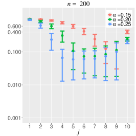
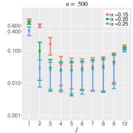
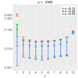
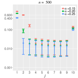
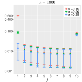
In the first experiment, we generate a sample of size $n$ from the uniform distribution on $S$ and calculate the estimator $\hat{V}$. We consider different sizes $m$ for the subsample $\mathcal{X}^{\prime}_{n}$ (different ways of splitting the sample) and different values of $\alpha$. Each setting is repeated $B=500$ times. Figure 2 shows the mean values $|\mu(S)-\hat{V}|/\mu(S)$ over the $B$ repeats (error bars represent one standard deviation). We do the same for $\mu(C_{\alpha}(\mathcal{X}_{n}))$ instead of $\hat{V}$.

Figure 2: Mean values of $|\mu(S)-\hat{V}|/\mu(S)$ over $B=500$ repeats and error bars representing one standard deviation (a base-10 log scale is used for the $Y$-axis). In the computation of $\hat{V}$ we have considered different sizes $m=[nj/10]$ for the subsample $\mathcal{X}^{\prime}_{n}$. The case $j=10$ corresponds to the plug-in estimator.

Bagging

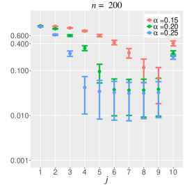
In the second experiment, we study the same scenarios as in the first experiment, and examine the strategy of performing the sample splitting multiple times. The new estimator, denoted $\hat{V}_{\rm bag}$, is obtained by computing ${\hat{V}}$ for $b=100$ random sample splittings and averaging these. This is a form of bagging, therefore the name. Figure 3 shows the mean values of $|\mu(S)-\hat{V}_{\rm bag}|/\mu(S)$ over the $B$ repeats. ($B=500$ as before.) As it can be seen, compared to Figure 2, this bagging technique reduces the variance of the error.

Figure 3: Mean values of $|\mu(S)-\hat{V}_{\rm bag}|/\mu(S)$ over $B=500$ repeats and error bars representing one standard deviation (a base-10 log scale is used for the $Y$-axis). The bagging was over $b=100$ sample splittings. In the computation of $\hat{V}$ we have considered different sizes $m=[nj/10]$ for the subsample $\mathcal{X}^{\prime}_{n}$. The case $j=10$ corresponds to $\hat{V}=\mu(C_{\alpha}(\mathcal{X}_{n}))$.

Confidence intervals

As mentioned before, the proposed method lends itself naturally to the computation of confidence intervals for $\mu(S)$ based on the computation of confidence intervals for $\tilde{p}$. We use the method of Wilson (1927) for that purpose. Results of the estimated coverage probability and estimated mean length of the confidence intervals for different nominal confidence levels are shown in Table 1. (This is just meant as a proof of concept since there are no other methods we know off to compare this with.)

	Level	0.50	0.55	0.60	0.65	0.70	0.75	0.80	0.85	0.90	0.95
$n=200$	Coverage	0.52	0.55	0.61	0.65	0.70	0.74	0.80	0.85	0.90	0.94
	Length	0.31	0.35	0.39	0.43	0.48	0.53	0.59	0.67	0.76	0.91
$n=500$	Coverage	0.50	0.55	0.60	0.64	0.69	0.74	0.81	0.87	0.91	0.95
	Length	0.11	0.13	0.14	0.16	0.18	0.20	0.22	0.25	0.28	0.34
$n=1000$	Coverage	0.50	0.55	0.58	0.64	0.68	0.73	0.77	0.82	0.89	0.94
	Length	0.06	0.07	0.08	0.08	0.09	0.10	0.12	0.13	0.15	0.18

Table 1: Coverage and length of the confidence interval for $\mu(S)$ based on a confidence interval for $\tilde{p}$. We split the sample in half (meaning, we used $m=n/2$) and used $\alpha=0.25$. Each setting is repeated $B=500$ times and what are shown are the averages of the $B$ repeats.

The convex case

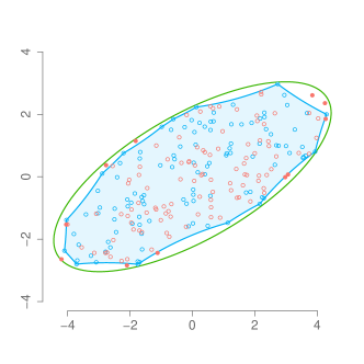
We replicated the study in (Baldin and Reiß, 2015) to compare the performance of our estimator $\hat{V}$ with that of the estimators discussed in that paper for the convex case. Data points are simulated for an ellipse, $S$, with center at the origin, major axis of length 10 and minor axis of length 4; see Figure 4 (left). More specifically, for different values of $n$, we generated $B=500$ samples from a Poisson spatial process over $S$ with constant intensity $\lambda=n/\mu(S)$. The size of each sample, $N$, is Poisson distributed with mean $n$. For the computation of $\hat{V}$ we randomly split each sample into two subsamples of equal size and compute the $\alpha$-convex hull of the first subsample with $\alpha=10$. We base our choice of $\alpha$ on the fact that, under the assumption of convexity, the $\alpha$-convex hull estimator works reasonably well for large values of $\alpha$. Figure 4 (right) shows, for the considered estimators, the RMSE normalized by the true area based on the $B=500$ Monte Carlo iterations for each $n$. We use the same notation as in (Baldin and Reiß, 2015). Our estimator $\hat{V}$ performs slightly better than the rate-optimal estimator based on sample splitting by Gayraud (1997), denoted by $\hat{\upsilon}_{G}$. The best performance corresponds to $\hat{\upsilon}_{oracle}$, altough its computation depends on the unknown intensity $\lambda$. The estimators $\hat{\upsilon}_{plugin}$ and $\hat{\upsilon}$, for the case of unknown intensity $\lambda$, also perform well. As already pointed out by Baldin and Reiß (2015), all these methods clearly outperform the results of other estimators that are not rate-optimal, such as the Lebesgue measure of the convex hull of the sample, denoted by $|\hat{C}|$, and the so-called naive oracle estimator $N/\lambda$.

Figure 4: Left: A random sample is generated on the ellipse $S$ in green and splitted into $\mathcal{X}^{\prime}_{n}$ (blue points) and $\mathcal{X}^{\prime\prime}_{n}$ (open and solid red points). The solid red points are the observations of $\mathcal{X}^{\prime\prime}_{n}$ that fall outside $C_{\alpha}(\mathcal{X}^{\prime}_{n})$, represented in blue for $\alpha=10$. Right: The RMSE (normalized by $\mu(S)$) of different estimators of $\mu(S)$, based on $B=500$ Monte Carlo iterations in each case.

5 Discussion

Choice of parameters. The first estimator we propose, just like the plug-in estimator, depends on the choice of $\alpha>0$. We proved our result (Theorem 2) under the assumption that $\alpha\leq r$, but in general $r$ is unknown. Also, although the theory works for any $\alpha$ thus chosen, in practice, an optimal choice for $\alpha$ may depend on the sample size. Under uniform sampling, in Rodríguez-Casal and Saavedra-Nieves (2014) is proposed a data-driven selector of $\alpha$, $\alpha_{n}$, such that, with probability one, satisfies $\alpha_{n}\leq r$ and $\alpha_{n}\to r$.

Extensions. We are confident that our proof arguments proceed with relatively minor modifications when $\partial S$ is piecewise smooth. However, our working condition (1) — which is equivalently expressed as a requirement on the reach of $\partial S$ — is simple and compact, and the resulting analysis already contains all the intricacies. A more substantial extension is to the setting of an unknown sampling distribution. This setting is considered in (Gayraud, 1997), where the sampling density is estimated by a standard kernel procedure, and that estimate is incorporated in the estimator of the volume. Although the methodology and theory developed in that paper do not apply directly, an adaptation to our setting (namely, to sets satisfying (1)) seems viable.

Perimeter. A parallel line of research tackles the problem of estimating the perimeter of $S$. In fact, this problem is also considered by Rényi and Sulanke (1964) and Bräker and Hsing (1998), still in the context of a convex support set in dimension $d=2$. More recently, in the same setting as ours here, but restricted to dimension $d=2$, Cuevas et al. (2012) study the perimeter of the sample $\alpha$-convex hull, while Arias-Castro and Rodríguez-Casal (2015) study the perimeter of the sample $\alpha$-shape. Parallel to the work of Korostelëv and Tsybakov (1993), and working with a similar model, we find the work of Kim and Korostelev (2000). We also mention a series of papers that consider the closely related problem of estimating the Minkowski content of the boundary of $S$, still under a similar model, making various regularity assumptions on $S$ (Cuevas et al., 2007; Pateiro-López and Rodríguez-Casal, 2009, 2008; Jiménez and Yukich, 2011). It would be interesting to obtain similar results for the problem of estimating the perimeter of $S$ under our setting or some of these other settings.

Acknowledgments

This work was partially supported by the US National Science Foundation (DMS 1513465) and by the Spanish Ministry of Economy and Competitiveness and ERDF funds (MTM2013-41383-P).

Appendix A Appendix: additional proofs

A.1 Rolling a ball inside a convex set

Definition 3.

For a set $S$ and $\alpha>0$, let $G_{\alpha}(S)$ denote the set of $x\in S$ with the property that there is an open ball $B$ of radius $\alpha$ such that $x\in B\subset S$.

Lemma 2.

If $S\subset\mathbb{R}^{d}$ is convex, then for any $\alpha>0$, $G_{\alpha}(S)$ is either empty or convex.

Proof.

Write $G$ for $G_{\alpha}(S)$. By definition (and the axiom of choice), for any $x\in S$ we may choose an open ball of radius $\alpha$, denoted $B_{x}$, such that $x\in B_{x}\subset S$. Suppose $S$ contains a ball of radius $\alpha$, for otherwise $G$ is empty and there is nothing else to prove. Take $x,y\in G$ and let $C$ denote the convex hull of $B_{x}\cup B_{y}$. On the one hand, $C\subset S$, because $B_{x}\cup B_{y}\subset S$ and $S$ is convex. On the other hand, for all $z\in C$, there is a ball $B$ of radius $\alpha$ such that $z\in B\subset C$. This is obvious from the fact that $C$ is the union of the cylinder with center rod $[xy]$ and radius $\alpha$ and the two half balls defined by $B_{x}$ and $B_{y}$ on each end, which can be expressed as

$$C=\bigcup_{t\in[x,y]}B(t,\alpha).$$ (33)

Hence, $C\subset G$, and in particular, $[xy]\subset G$ since $[xy]\subset C$. This being true for all $x,y\in G$, we conclude that $G$ is indeed convex. ∎

A.2 Proof of Theorem 3

The arguments are only sketched and more details can be found in (Pateiro-Lopez, 2008).

Before proving Theorem 3, we need to introduce some notation. The distance between $x\in\mathbb{R}^{d}$ and $S\subset\mathbb{R}^{d}$ is defined as $\operatorname{dist}(x,S)=\inf_{s\in S}\|x-s\|$. Given a unit vector $u$ and an angle $\theta\in[0,\pi/2]$, consider the infinite cone with apex $x$, axis $u$ and aperture $2\theta$ defined by

$$C_{u}^{\theta}(x)=\{z\in\mathbb{R}^{d},z\neq x:\left\langle{z-x},u\right\rangle\geq{\|z-x\|}\cos\theta\}.$$

Note that the notation is slightly different from the one we used in Section 2. For $h>0$, consider the finite cone obtained by intersecting an infinite cone with a ball of radius $h$ centered at its apex, $C_{u,h}^{\theta}(x)=C_{u}^{\theta}(x)\cap B(x,h)$. For $x\in\mathbb{R}^{d}$ and $r>0$, let $\mathcal{E}_{x,r}=\{{B}(y,r):y\in{B}(x,r)\}$.

Definition 4.

The family of sets $\mathcal{U}$ is said to be unavoidable for another family of sets $\mathcal{E}$ if, for all $E\in\mathcal{E}$, there exists $U\in\mathcal{U}$ such that $U\subset E$.

Lemma 3.

Under the conditions of Theorem 3 (and recalling the definition of $\delta$ there), for any $x\in S$ such that $\operatorname{dist}(x,\partial S)>\alpha_{n}/2$, there exists a finite family $\mathcal{U}_{x,\alpha_{n}}$ with at most $m_{1}$ elements, unavoidable for $\mathcal{E}_{x,\alpha_{n}}$ and that satisfies

$$P_{X}(U)\geq L_{1}\alpha_{n}^{d},\quad\forall U\in\mathcal{U}_{x,\alpha_{n}},$$

where $m_{1}\geq 1$ depends only on $d$ and $L_{1}>0$ only on $(d,\delta)$.

Proof.

The case $d=1$ is handled separately. For $x\in\mathbb{R}$ under the stated conditions let us consider the unavoidable family $\mathcal{U}_{x,\alpha_{n}}=\{[x-\alpha_{n}/2,x],[x,x+\alpha_{n}/2]\}$. The result holds for $L_{1}=\delta/2$. For the case $d=2$, see Proposition 1 of (Pateiro-López and Rodríguez-Casal, 2013). Let us then assume that $d\geq 3$ and fix $\theta=\pi/6$. There exists a finite family $W$, with $m_{1}$ unit vectors ($m_{1}$ dependent only on $d$), such that we can cover $B(x,\alpha_{n})$ by the cones $C_{u,{\alpha_{n}}}^{\theta}(x)$, with $u\in W$. The family $\mathcal{U}_{x,\alpha_{n}}=\{C_{u,\alpha_{n}/2}^{\theta}(x),\ u\in W\}$ is unavoidable for $\mathcal{E}_{x,\alpha_{n}}$. For each $u\in W$,

$$P_{X}\left(C_{u,\alpha_{n}/2}^{\theta}(x)\right)\geq\delta\mu\left(C_{u,\alpha_{n}/2}^{\theta}(x)\cap S\right)=\delta\mu\left(C_{u,\alpha_{n}/2}^{\theta}(x)\right)$$ (34)

where the equality comes from the fact that $\operatorname{dist}(x,\partial S)>\alpha_{n}/2$. Finally,

$$\mu\left(C_{u,\alpha_{n}/2}^{\theta}(x)\right)\geq\mu(B(x,\alpha_{n}/2))/m_{1}=\omega_{d}\left(\alpha_{n}/2\right)^{d}/m_{1},$$ (35)

where $\omega_{d}$ denotes the Lebesgue measure of the unit ball in $\mathbb{R}^{d}$. The proof is complete with $L_{1}=\delta\omega_{d}/(2^{d}m_{1})$. ∎

Lemma 4.

Under the conditions of Theorem 3 (and recalling the definition of $r$ and $\delta$ there), for any $x\in S$ such that $\operatorname{dist}(x,\partial S)\leq\alpha_{n}/2$, there exists a finite family $\mathcal{U}_{x,\alpha_{n}}$ with at most $m_{2}$ elements, unavoidable for $\mathcal{E}_{x,\alpha_{n}}$ and that satisfies

$$P_{X}(U)\geq L_{2}\alpha_{n}^{(d-1)/2}\operatorname{dist}(x,\partial S)^{(d+1)/2},\quad\forall U\in\mathcal{U}_{x,\alpha_{n}},$$

where $m_{2}\geq 1$ depends only on $d$ and $L_{2}>0$ only on $(d,r,\delta)$.

Proof.

Let $x\in S$ such that $\operatorname{dist}(x,\partial S)\leq\alpha_{n}/2$. We denote $\rho=\operatorname{dist}(x,\partial S)$. For $d=1$ consider the unavoidable family $\mathcal{U}_{x,\alpha_{n}}=\{[x-\rho,x],[x,x+\rho]\}$ and the result holds for $L_{2}=\delta$. For the case $d=2$, see Proposition 2 of (Pateiro-López and Rodríguez-Casal, 2013). Let us assume that $d\geq 3$. Using the rolling condition, let $P_{\Gamma}x$ be the metric projection of $x$ onto $\Gamma:=\partial S$ and $\eta$ the outward pointing unit normal vector at $P_{\Gamma}x$. By the fact that $S^{\mathsf{c}}$ satisfies the $r$-rolling ball condition, we have that $B(P_{\Gamma}x-r\eta,r)\subset S$. Thus, given $\mathcal{U}_{x,\alpha_{n}}$ an unavoidable family of sets for $\mathcal{E}_{x,\alpha_{n}}$, we have that

$$P_{X}(U)\geq\delta\mu(U\cap S)\geq\delta\mu(U\cap B(P_{\Gamma}x-r\eta,r))$$ (36)

for all $U\in\mathcal{U}_{x,\alpha_{n}}$. We can assume, without loss of generality, that $x$ is the origin and $\eta=-e_{d}$, where $e_{d}$ denotes the $d$-th canonical basis vector. Then, the problem reduces to defining a suitable family of sets $\mathcal{U}_{0,\alpha_{n}}$ unavoidable for $\mathcal{E}_{0,\alpha_{n}}$ and giving a lower bound for $\mu(U\cap B((r-\rho)e_{d},r))$ independent of $U\in\mathcal{U}_{0,\alpha_{n}}$. We partition $B(0,\alpha_{n})$ into the following two sets

$$G_{\alpha_{n}}=\left\{y\in B(0,\alpha_{n}):\ \left\langle y,e_{d}\right\rangle\geq-\left\|y\right\|/2\right\},\quad F_{\alpha_{n}}=\left\{y\in B(0,\alpha_{n}):\ \left\langle y,e_{d}\right\rangle<-\left\|y\right\|/2\right\}.$$ (37)

In order to simplify the notation, we write $C_{u}^{\theta}$ and $C_{u,h}^{\theta}$ to refer to $C_{u}^{\theta}(x)$ and $C_{u,h}^{\theta}(x)$ for $x=0$.

First, let us consider $G_{\alpha_{n}}$. Fix $\theta=\pi/6$ and $\gamma\in(0,\pi/6)$, say $\gamma=\pi/7$. There exists a finite family $W^{G}$, with $m^{G}$ unit vectors (depending only on $d$), with the property that for all $y\in G_{\alpha_{n}}$ there exists $u\in W^{G}$ such that $C_{u,\alpha_{n}}^{\theta}\subset B(y,\alpha_{n})$ and $\left\langle u,e_{d}\right\rangle\geq-\sin\gamma$. Let $H_{0}=\{x\in\mathbb{R}^{d}:\langle x,e_{d}\rangle\geq 0\}$. There is an absolute angle $\tilde{\theta}>0$ with the property that, for each unit vector $u$ with $\left\langle u,e_{d}\right\rangle\geq-\sin\gamma$ there exists a unit vector $\tilde{u}$ such that $C_{\tilde{u}}^{\tilde{\theta}}\subset C_{u}^{\theta}\cap H_{0}$. Now, for $\psi=\sqrt{\rho(2r-\rho)}$ and for each $u\in W^{G}$,

$$C_{u,\alpha_{n}}^{\theta}\cap B((r-\rho)e_{d},r)\supset C_{u,\alpha_{n}}^{\theta}\cap H_{0}\cap B(0,\psi)\supset C_{\tilde{u},\alpha_{n}}^{\tilde{\theta}}\cap B(0,\psi)=C_{\tilde{u},\tau_{n}}^{\tilde{\theta}},$$ (38)

where $\tau_{n}:=\min(\psi,\alpha_{n})$. The ball $B(0,\tau_{n})$ can be covered by a finite number $m$ (depending only on $d$) of cones $C_{\tilde{u},\tau_{n}}^{\tilde{\theta}}$, with varying $\tilde{u}$. Using that $\alpha_{n}\leq r$ and $\rho\leq\alpha_{n}/2$, we have that

$$\mu\left(B(0,\tau_{n})\right)\geq w_{d}\alpha_{n}^{(d-1)/2}\rho^{(d+1)/2}$$ (39)

and, therefore,

$$\mu(C_{u,\alpha_{n}}^{\theta}\cap B((r-\rho)e_{d},r))\geq L^{G}\alpha_{n}^{(d-1)/2}\rho^{(d+1)/2},$$ (40)

where $L^{G}:=w_{d}/m>0$ only depends on $d$.

Now, let us consider $F_{\alpha_{n}}$. First, we define the set

$$C_{\ddagger}=\{x\in\mathbb{R}^{d}:\ -h_{1}\leq\left\langle x,e_{d}\right\rangle\leq 0\}\cap B(-\alpha_{n}e_{d},\alpha_{n}),$$ (41)

where $h_{1}:={\rho(2r-\rho)}/(2(r+\alpha_{n}-\rho))$; see Figure 5 (left). It can be proved that $C_{\ddagger}\subset B((r-\rho)e_{d},r)$ and

$$\mu(C_{\ddagger})\geq\frac{\omega_{d-1}}{(d+1)2^{(d-1)/2}}\alpha_{n}^{(d-1)/2}\rho^{(d+1)/2}.$$ (42)

For $\theta\in[0,\pi/2]$ and a unit vector $u\in\mathbb{R}^{d-1}$, let $Q_{u}^{\theta}=\left\{x\in\mathbb{R}^{d}:\ x_{-d}\in C_{u}^{\theta}\right\}$, where $x_{-d}$ denotes the vector $x$ without the last component; see Figure 5 (right).

Figure 5: Left, in gray set $C_{\ddagger}$ in $\mathbb{R}^{3}$. Right, example of set $Q_{u}^{\theta}$ in $\mathbb{R}^{3}$.

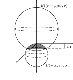
We will prove that we can define an unavoidable family with sets of the form $Q_{u}^{\theta}\cap C_{\ddagger}$, all with the same Lebesgue measure; see Figure 6.

Figure 6: Example of set $Q_{u}^{\theta}\cap C_{\ddagger}$ in $\mathbb{R}^{3}$.

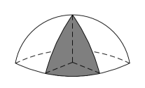
Fix $\theta=\pi/6$. There exists a finite family $W^{F}$, with $m^{F}$ unit vectors in $\mathbb{R}^{d-1}$ (depending only on $d$), with the property that for all $y\in F_{\alpha_{n}}$ there exists $u\in W^{F}$ such that $Q_{u}^{\theta}\cap C_{\ddagger}\subset B(y,\alpha_{n})$. Finally, we use that $C_{\ddagger}\subset B((r-\rho)e_{d},r)$, the fact that $C_{\ddagger}$ can be covered by the sets $Q_{u}^{\theta}\cap C_{\ddagger}$ with $u\in W^{F}$, and (42), to obtain the following sequence of inequalities

$$\mu\left(Q_{u}^{\theta}\cap C_{\ddagger}\cap B((r-\rho)e_{d},r)\right)=\mu(Q_{u}^{\theta}\cap C_{\ddagger})\geq\mu(C_{\ddagger})/m^{F}\geq L^{F}\alpha_{n}^{(d-1)/2}\rho^{(d+1)/2},$$ (43)

where $L^{F}:=\frac{\omega_{d-1}}{m^{F}(d+1)2^{(d-1)/2}}$ depends only on $d$.

We finish by defining the family

$$\mathcal{U}_{0,\alpha_{n}}=\{C_{u,\alpha_{n}}^{\theta}:u\in W^{G}\}\cup\{Q_{u}^{\theta}\cap C_{\ddagger}:u\in W^{F}\}.$$ (44)

This completes the proof of the lemma, with $m_{2}:=m^{G}+m^{F}$ depending only on $d$ and $L_{2}:=\delta\min(L^{G},L^{F})$ only on $(d,\delta)$. ∎

Proof of Theorem 3.

Let $S_{n}=C_{\alpha_{n}}(\mathcal{X}_{n})$. With probability one, $\mathcal{X}_{n}\subset S$, which implies $S_{n}\subset S$ and

$$\operatorname{\mathbb{E}}\big{[}\mu(S_{n}\triangle S)\big{]}=\mathbb{E}\big{[}\mu(S\setminus S_{n})\big{]}=\int_{S}{P(\exists y\in{B}(x,\alpha_{n}):{B}(y,\alpha_{n})\cap\mathcal{X}_{n}=\emptyset)\mu({\rm d}x)}.$$ (45)

For each $x\in S$ we choose a finite family $\mathcal{U}_{x,\alpha_{n}}$ unavoidable for $\mathcal{E}_{x,\alpha_{n}}$. Then, as a consequence of Definition 4, we have

$$\begin{split}P(\exists y\in{B}(x,\alpha_{n}):{B}(y,\alpha_{n})\cap\mathcal{X}_{n}=\emptyset)\leq\sum_{U\in\mathcal{U}_{x,\alpha_{n}}}(1-P_{X}(U))^{n}\leq\sum_{U\in\mathcal{U}_{x,\alpha_{n}}}\exp\left(-nP_{X}(U)\right).\end{split}$$ (46)

We partition $S$ into two subsets

$$S_{1}=\left\{x\in S:\ \ \operatorname{dist}(x,\partial S)>\alpha_{n}/2\right\},\quad S_{2}=\left\{x\in S:\ \ \operatorname{dist}(x,\partial S)\leq\alpha_{n}/2\right\}.$$ (47)

For those $x\in S_{1}$, choose a family as in Lemma 3, to get

$$\int_{S_{1}}{\sum_{U\in\mathcal{U}_{x,\alpha_{n}}}\exp(-nP_{X}(U))\mu({\rm d}x)}\leq\int_{S_{1}}{m_{1}\exp(-nL_{1}\alpha_{n}^{d})\mu({\rm d}x)}=O\left(\textnormal{e}^{-L_{1}n\alpha_{n}^{d}}\right),$$ (48)

where $m_{1}$ and $L_{1}$ are defined in Lemma 3. For those $x\in S_{2}$, choose a family as in Lemma 4, and follow the same arguments as in (Pateiro-López and Rodríguez-Casal, 2013), to get

$$\begin{split}\int_{S_{2}}{\sum_{U\in\mathcal{U}_{x,\alpha_{n}}}\exp(-nP_{X}(U))\mu({\rm d}x)}&\leq\int_{S_{2}}{m_{2}\exp\left(-L_{2}n\alpha_{n}^{(d-1)/2}\operatorname{dist}(x,\partial S)^{(d+1)/2}\right)\mu({\rm d}x)}\\ &=O\left(\alpha_{n}^{-(d-1)/(d+1)}n^{-2/(d+1)}\right).\end{split}$$ (49)

It follows from (48) and (49), and all the derivations that precede these, that

$$\operatorname{\mathbb{E}}\big{[}\mu(C_{\alpha_{n}}(\mathcal{X}_{n})\triangle S)\big{]}=O\left(\textnormal{e}^{-L_{1}n\alpha_{n}^{d}}+\alpha_{n}^{-(d-1)/(d+1)}n^{-2/(d+1)}\right).$$ (50)

Since $\alpha_{n}$ is bounded by $r$ and $n\alpha_{n}^{d}/\log n\to\infty$, we have $\textnormal{e}^{-L_{1}n\alpha_{n}^{d}}=o(\alpha_{n}^{-(d-1)/(d+1)}n^{-2/(d+1)})$, and this completes the proof. ∎

References

- Arias-Castro and Rodríguez-Casal (2015) Arias-Castro, E. and A. Rodríguez-Casal (2015). On estimating the perimeter using the alpha-shape. arXiv preprint arXiv:1507.00065. To appear in the Annales de l’Institut Henri Poincaré.
- Baldin and Reiß (2015) Baldin, N. and M. Reiß (2015). Unbiased estimation of the volume of a convex body. arXiv preprint arXiv:1502.05510. To appear in Stochastic Processes and their Applications.
- Bräker and Hsing (1998) Bräker, H. and T. Hsing (1998). On the area and perimeter of a random convex hull in a bounded convex set. Probab. Theory Related Fields 111(4), 517–550.
- Cuevas et al. (2012) Cuevas, A., R. Fraiman, and B. Pateiro-López (2012). On statistical properties of sets fulfilling rolling-type conditions. Adv. Appl. Probab. 44(2), 311–329.
- Cuevas et al. (2007) Cuevas, A., R. Fraiman, and A. Rodríguez-Casal (2007). A nonparametric approach to the estimation of lengths and surface areas. Ann. Statist. 35(3), 1031–1051.
- Edelsbrunner et al. (1983) Edelsbrunner, H., D. G. Kirkpatrick, and R. Seidel (1983). On the shape of a set of points in the plane. IEEE Trans. Inform. Theory 29(4), 551–559.
- Federer (1959) Federer, H. (1959). Curvature measures. Trans. Amer. Math. Soc. 93, 418–491.
- Gayraud (1997) Gayraud, G. (1997). Estimation of functionals of density support. Mathematical Methods of Statistics 6(1), 26–46.
- Hoeffding (1963) Hoeffding, W. (1963). Probability inequalities for sums of bounded random variables. J. Amer. Statist. Assoc. 58, 13–30.
- Jiménez and Yukich (2011) Jiménez, R. and J. E. Yukich (2011). Nonparametric estimation of surface integrals. Ann. Statist. 39(1), 232–260.
- Kim and Korostelev (2000) Kim, J.-C. and A. Korostelev (2000). Estimation of smooth functionals in image models. Mathematical Methods of Statistics 9(2), 140–159.
- Korostelëv and Tsybakov (1993) Korostelëv, A. P. and A. B. Tsybakov (1993). Minimax theory of image reconstruction, Volume 82 of Lecture Notes in Statistics. New York: Springer-Verlag.
- Mammen and Tsybakov (1995) Mammen, E. and A. B. Tsybakov (1995). Asymptotical minimax recovery of sets with smooth boundaries. Ann. Statist. 23(2), 502–524.
- Pateiro-Lopez (2008) Pateiro-Lopez, B. (2008). Set estimation under convexity type restrictions. Ph. D. thesis, Universidad de Santiago de Compostela.
- Pateiro-López and Rodríguez-Casal (2008) Pateiro-López, B. and A. Rodríguez-Casal (2008). Length and surface area estimation under smoothness restrictions. Adv. in Appl. Probab. 40(2), 348–358.
- Pateiro-López and Rodríguez-Casal (2009) Pateiro-López, B. and A. Rodríguez-Casal (2009). Surface area estimation under convexity type assumptions. J. Nonparametr. Stat. 21(6), 729–741.
- Pateiro-López and Rodríguez-Casal (2013) Pateiro-López, B. and A. Rodríguez-Casal (2013). Recovering the shape of a point cloud in the plane. TEST 22(1), 19–45.
- Perkal (1956) Perkal, J. (1956). Sur les ensembles -convexes. Colloq. Math. 4, 1–10.
- Rényi and Sulanke (1964) Rényi, A. and R. Sulanke (1964). Über die konvexe Hülle von zufällig gewählten Punkten. II. Z. Wahrscheinlichkeitstheorie und Verw. Gebiete 3, 138–147 (1964).
- Rodríguez-Casal (2007) Rodríguez-Casal, A. (2007). Set estimation under convexity type assumptions. Ann. Henri Poincaré 43(6), 763–774.
- Rodríguez-Casal and Saavedra-Nieves (2014) Rodríguez-Casal, A. and P. Saavedra-Nieves (2014). A fully data-driven method for estimating density level sets. arXiv preprint arXiv:1411.7687.
- Walther (1997) Walther, G. (1997). Granulometric smoothing. The Annals of Statistics 25(6), pp. 2273–2299.
- Walther (1999) Walther, G. (1999). On a generalization of Blaschke’s rolling theorem and the smoothing of surfaces. Math. Methods Appl. Sci. 22(4), 301–316.
- Wilson (1927) Wilson, E. B. (1927). Probable inference, the law of succession, and statistical inference. Journal of the American Statistical Association 22(158), 209–212.
- Yu (1997) Yu, B. (1997). Assouad, Fano, and Le Cam. In Festschrift for Lucien Le Cam, pp. 423–435. New York: Springer.