Convergence of a decoupled mixed FEM for the dynamic Ginzburg–Landau equations in nonsmooth domains with incompatible initial data

Abstract

In this paper, we propose a fully discrete mixed finite element method for solving the time-dependent Ginzburg–Landau equations, and prove the convergence of the finite element solutions in general curved polyhedra, possibly nonconvex and multi-connected, without assumptions on the regularity of the solution. Global existence and uniqueness of weak solutions for the PDE problem are also obtained in the meantime. A decoupled time-stepping scheme is introduced, which guarantees that the discrete solution has bounded discrete energy, and the finite element spaces are chosen to be compatible with the nonlinear structure of the equations. Based on the boundedness of the discrete energy, we prove the convergence of the finite element solutions by utilizing a uniform $L^{3+\delta}$ regularity of the discrete harmonic vector fields, establishing a discrete Sobolev embedding inequality for the Nédélec finite element space, and introducing a $\ell^{2}(W^{1,3+\delta})$ estimate for fully discrete solutions of parabolic equations. The numerical example shows that the constructed mixed finite element solution converges to the true solution of the PDE problem in a nonsmooth and multi-connected domain, while the standard Galerkin finite element solution does not converge.

1 Introduction

The time-dependent Ginzburg–Landau equation (TDGL) is a macroscopic phenomenological model for the superconductivity phenomena in both low and high temperatures [25, 27, 18, 38], and has been widely accepted in the numerical simulation of transition and vortex dynamics of both type-I and type-II superconductors [22, 31]. In a non-dimensionalization form, the TDGL is given by

$$\eta\frac{\partial\psi}{\partial t}+i\eta\kappa\psi\phi+\bigg{(}\frac{i}{\kappa}\nabla+\mathbf{A}\bigg{)}^{2}\psi+(|\psi|^{2}-1)\psi=0,$$ (1.1)

$$\frac{\partial\mathbf{A}}{\partial t}+\nabla\phi+\nabla\times(\nabla\times{\bf A})+{\rm Re}\bigg{[}\overline{\psi}\bigg{(}\frac{i}{\kappa}\nabla+\mathbf{A}\bigg{)}\psi\bigg{]}=\nabla\times{\bf H},$$ (1.2)

where the order parameter $\psi$ is complex scalar-valued, the electric potential $\phi$ is real scalar-valued and magnetic potential ${\bf A}$ is real vector-valued; $\eta>0$ and $\kappa>0$ are physical parameters, and ${\bf H}$ is a time-independent external magnetic field. In a domain $\Omega\subset\mathbb{R}^{3}$ occupied by a superconductor, the following physical boundary conditions are often imposed:

$$\Big{(}\frac{i}{\kappa}\nabla\psi+\mathbf{A}\psi\Big{)}\cdot{\bf n}=0 \mbox{on}\,\,\,\,\partial\Omega,$$ (1.3)

$${\bf n}\times{\bf B}={\bf n}\times{\bf H} \mbox{on}\,\,\,\,\partial\Omega,$$ (1.4)

$${\bf E}\cdot{\bf n}=0 \mbox{on}\,\,\,\,\partial\Omega,$$ (1.5)

where $\mathbf{n}$ denotes the unit normal vector on the boundary of the domain, ${\bf B}=\nabla\times{\bf A}$ and ${\bf E}=-\partial_{t}{\bf A}-\nabla\phi$ denote the induced magnetic and electric fields, respectively.

Besides (1.1)-(1.2), an additional gauge condition is needed for the uniqueness of the solution $(\psi,\phi,{\bf A})$. Under the gauge $\phi=-\nabla\cdot{\bf A}$, the TDGL reduces to

$$\eta\frac{\partial\psi}{\partial t}-i\eta\kappa\psi\nabla\cdot{\bf A}+\bigg{(}\frac{i}{\kappa}\nabla+\mathbf{A}\bigg{)}^{2}\psi+(|\psi|^{2}-1)\psi=0,$$ (1.6)

$$\frac{\partial\mathbf{A}}{\partial t}+\nabla\times(\nabla\times{\bf A})-\nabla(\nabla\cdot{\bf A})+{\rm Re}\bigg{[}\overline{\psi}\bigg{(}\frac{i}{\kappa}\nabla+\mathbf{A}\bigg{)}\psi\bigg{]}=\nabla\times{\bf H},$$ (1.7)

and the boundary conditions can be written as

$$\nabla\psi\cdot{\bf n}=0 \mbox{on}\,\,\,\,\partial\Omega,$$ (1.8)

$${\bf n}\times(\nabla\times{\bf A})={\bf n}\times{\bf H} \mbox{on}\,\,\,\,\partial\Omega,$$ (1.9)

$${\bf A}\cdot{\bf n}=0 \mbox{on}\,\,\,\,\partial\Omega.$$ (1.10)

Given the initial conditions

$$\psi(x,0)=\psi_{0}(x)\quad\mbox{and}\quad{\bf A}(x,0)={\bf A}_{0}(x),\quad\mbox{for}\,\,x\in\Omega,$$ (1.11)

the solution $(\psi,{\bf A})$ can be solved from (1.6)-(1.11). Other gauges can also be used, and the solutions under different gauges are equivalent in the sense that they produce the same quantities of physical intereset [14, 38], such as the superconducting density $|\psi|^{2}$ and the magnetic field ${\bf B}$.

In a smooth domain, well-posedness of (1.6)-(1.11) has been proved in [14] and convergence of the Galerkin finite element method (FEM) was proved in [13, 23] with different time discretizations by assuming that the PDE’s solution is smooth enough, e.g. ${\bf A}\in L^{\infty}(0,T;{\bf H}^{1})\cap L^{2}(0,T;{\bf H}^{2})$. In a nonsmooth domain such as a curved polyhedron, the magnetic potential ${\bf A}$ may be only in $L^{\infty}(0,T;{\bf H}({\rm curl,div}))\cap L^{2}(0,T;{\bf H}^{1/2+\delta})$, where $\delta>0$ can be arbitrarily small (depending on the angle of the edges or corners of the domain), and so the Galerkin finite element solution may not converge to the solution of (1.6)-(1.7). Some mixed FEMs were proposed in [12, 24], and the numerical simulations in [24] show better results in nonsmooth domains, compared with the Galerkin FEM. Some discrete gauge invariant numerical methods [19, 21] are also promising to approximate the solution correctly. Convergence of these numerical methods have been proved in the case that the PDE’s solution is smooth enough. However, whether the numerical solutions converge to the PDE’s solution in nonsmooth domains where the magnetic potential is only in $L^{\infty}(0,T;{\bf H}({\rm curl,div}))\cap L^{2}(0,T;{\bf H}^{1/2+\delta})$ is still unknown. Another problem is that the initial data ${\bf A}_{0}$ are often incompatible with the boundary condition (1.9) (see the numerical examples in [5, 13, 32], where ${\bf n}\times(\nabla\times{\bf A}_{0})=0$ but ${\bf n}\times{\bf H}\neq 0$), and this also leads to low regularity of the solution.

Numerical analysis of the TDGL under the zero electric potential gauge $\phi=0$ has also been done in many works [5, 28, 26, 33, 39, 40, 41, 43]; also see the review paper [20]. Since $\|\nabla\times{\bf A}\|_{L^{2}}$ is not equivalent to $\|\nabla{\bf A}\|_{L^{2}}$, both theoretical and numerical analysis are difficult under this gauge without extra assumptions on the regularity of the PDE’s solution. Again, convergence of these numerical methods have been proved in the case that the PDE’s solution is smooth enough.

Under either gauge, convergence of the numerical solutions has not been proved in nonsmooth domains such as general curved polyhedra, possibly nonconvex and multi-connected. Meanwhile, correct numerical approximations of the TDGL in domains with edges and corners are important for physicists and engineers [5, 6, 40]. The difficulty of the problem is to control the nonlinear terms in the equations only based on the a priori estimates of the finite element solution. In this paper, we introduce a decoupled mixed FEM for solving (1.6)-(1.10) which guarantees that the discrete solution has bounded discrete energy, and prove convergence of the fully discrete finite element solution in general curved polyhedra without assumptions on the regularity of the PDE’s solution. We control the nonlinear terms by proving a uniform $L^{3+\delta}$ regularity for the discrete harmonic vector fields in curved polyhedra, establishing a discrete Sobolev compact embedding inequality ${\bf H}_{h}({\rm curl,div})\hookrightarrow\hookrightarrow{\bf L}^{3+\delta}$ for the functions in the Nédélec element space, and introducing a $\ell^{2}(W^{1,3+\delta})$ estimate for fully discrete finite element solutions of parabolic equations, where $\delta>0$ is some constant which depends on the given domain.

2 Main results

2.1 A decoupled mixed FEM with bounded discrete energy

In this subsection, we introduce our assumptions on the domain and define the fully discrete finite element method to be considered in this paper. Then we introduce a discrete energy function (different from the free energy) and sketch a proof for a basic energy inequality satisfied by the finite element solution.

Definition 2.1

A curved polyhedron (or polygon) is a bounded Lipschitz domain $\Omega\subset\mathbb{R}^{3}$ (or $\Omega\subset\mathbb{R}^{2}$), possibly nonconvex and multi-connected, such that its boundary is locally $C^{\infty}$-isomorphic to the boundary of a polyhedron [10], and there are $\mathfrak{M}$ pieces of surfaces $\Sigma_{1}$, $\cdots$, $\Sigma_{\mathfrak{M}}$ transversal to $\partial\Omega$ such that $\Sigma_{i}\cap\Sigma_{j}=\emptyset$ for $i\neq j$ and the domain $\Omega_{0}:=\Omega\backslash\Sigma$ is simply connected, where $\Sigma=\cup_{j=1}^{\mathfrak{M}}\Sigma_{j}$ (see Figure 1) .

Remark 2.1

The integer $\mathfrak{M}$ is often referred to as the first Betti number of the domain. The existence of the surfaces $\Sigma_{j}$, $j=1,\cdots,\mathfrak{M}$, is only needed in the analysis of the finite element solutions by using the Hodge decomposition [30]. One does not need to know these surfaces in practical computation.

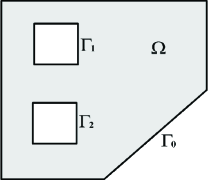
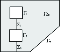
Figure 1: Illustration of the domain ($\Omega$ is the shadow region).

Assumptions 2.1.    We assume that $\Omega\subset\mathbb{R}^{3}$ is a curved polyhedron which is partitioned into quasi-uniform tetrahedra. For any given integers

$$r\geq 1\quad\mbox{and}\quad k\geq 2r-1,$$ (2.1)

we denote by ${\mathbb{S}}_{h}^{r}$ the complex-valued Lagrange finite element space of degree $\leq r$, denote by ${\mathbb{V}}_{h}^{k+1}$ the real-valued Lagrange finite element space of degree $\leq k+1$, and let ${\mathbb{N}}_{h}^{k}$ be either the Nédélec 1st-kind H(curl) element space of order $k$ [34] or the Nédélec 2nd-kind H(curl) element space of degree $\leq k$ [35] (also see page 60 of [4]).  

Let the time interval $[0,T]$ be partitioned into $0=t_{0}<t_{1}<\cdots<t_{N}$ uniformly, with $\tau=t_{n+1}-t_{n}$. For any given functions $f_{n}$, $n=0,1,\cdots,N$, we define its discrete time derivative as

$$D_{\tau}f^{n+1}:=(f^{n+1}-f^{n})/\tau,\quad n=0,1,\cdots,N-1.$$

We introduce a decoupled backward Euler scheme for solving (1.6)-(1.7):

$$\eta D_{\tau}\psi^{n+1}-i\eta\kappa\Theta(\psi^{n})\nabla\cdot{\bf A}^{n}+\bigg{(}\frac{i}{\kappa}\nabla+{\bf A}^{n+1}\bigg{)}^{2}\psi^{n+1}+(|\psi^{n+1}|^{2}-1)\psi^{n+1}=0,$$ (2.2)

$$D_{\tau}{\bf A}^{n+1}-\nabla(\nabla\cdot{\bf A}^{n+1})+\nabla\times(\nabla\times{\bf A}^{n+1})+{\rm Re}\bigg{[}\overline{\psi}^{n}\bigg{(}\frac{i}{\kappa}\nabla+{\bf A}^{n}\bigg{)}\psi^{n}\bigg{]}=\nabla\times{\bf H},$$ (2.3)

where we have used a cut-off function

$$\Theta(z):=z/\max(|z|,1),\quad\forall~{}z\in\mathbb{C},$$ (2.4)

which satisfies $\Theta(z)=z$ if $|z|\leq 1$.

For any given integers $r$ and $k$ which satisfy the condition (2.1), we solve (2.2) by the Galerkin FEM and solve (2.3) by a mixed FEM. Let $(\psi_{h}^{0},{\bf A}_{h}^{0}):=(\psi_{0},{\bf A}_{0})$ at the initial time step and define $\phi_{h}^{0}:=-\nabla\cdot{\bf A}_{0}$. We look for $\psi_{h}^{n+1}\in{\mathbb{S}}_{h}^{r}$ and $(\phi_{h}^{n+1},{\bf A}_{h}^{n+1})\in{\mathbb{V}}_{h}^{k+1}\times{\mathbb{N}}_{h}^{k}$, $n=0,1,\cdots,N-1$, satisfying the equations

$$(\eta D_{\tau}\psi_{h}^{n+1},\varphi_{h})+\bigg{(}\bigg{(}\frac{i}{\kappa}\nabla+{\bf A}_{h}^{n+1}\bigg{)}{\psi}_{h}^{n+1}\,,\bigg{(}\frac{i}{\kappa}\nabla+{\bf A}_{h}^{n+1}\bigg{)}\varphi_{h}\bigg{)}$$

$$\quad+((|\psi_{h}^{n+1}|^{2}-1)\psi_{h}^{n+1},\varphi_{h})=-(i\eta\kappa\Theta(\psi_{h}^{n})\phi_{h}^{n},\varphi_{h})\,, \forall\,\varphi_{h}\in{\mathbb{S}}_{h}^{r},$$ (2.5)

$$(\phi_{h}^{n+1},\chi_{h})-({\bf A}_{h}^{n+1},\nabla\chi_{h})=0\,, \forall\,\chi_{h}\in{\mathbb{V}}_{h}^{k+1},$$ (2.6)

$$(D_{\tau}{\bf A}_{h}^{n+1},{\bf a}_{h})+(\nabla\phi_{h}^{n+1}\,,{\bf a}_{h})+(\nabla\times{\bf A}_{h}^{n+1}\,,\nabla\times{\bf a}_{h})$$

$$=({\bf H}\,,\nabla\times{\bf a}_{h})-{\rm Re}\bigg{(}\overline{\psi}_{h}^{n}\bigg{(}\frac{i}{\kappa}\nabla+{\bf A}_{h}^{n}\bigg{)}\psi_{h}^{n},{\bf a}_{h}\bigg{)}\,, \forall\,{\bf a}_{h}\in{\mathbb{N}}_{h}^{k}.$$ (2.7)

After solving $\psi_{h}^{n+1}$, $\phi_{h}^{n+1}$ and ${\bf A}_{h}^{n+1}$ from the equations above, the magnetic and electric fields can be computed by ${\bf B}_{h}^{n+1}=\nabla\times{\bf A}_{h}^{n+1}$ and ${\bf E}_{h}^{n+1}=-D_{\tau}{\bf A}_{h}^{n+1}-\nabla\phi_{h}^{n+1}$.

Remark 2.2

For simplicity, we have chosen $(\psi_{h}^{0},{\bf A}_{h}^{0})=(\psi_{0},{\bf A}_{0})$ at the initial step, which are not finite element functions. Due to the nonlinearities and the choice of the initial data, some integrals in (2.5) and (2.7) may need to be evaluated numerically in practical computations. In this paper, we focus on the analysis of the discretization errors of the finite element method and assume that all the integrals are evaluated accurately.

Remark 2.3

Since we have not assumed any extra regularity of the PDE’s solution, we need the condition (2.1) to be compatible with the nonlinear structure of the equations in order to control a nonlinear term arising from (2.5) (see (3.4) for the details). If the PDE’s solution is smooth enough, (e.g. consider the problem in a smooth domain), then the condition (2.1) can be relaxed.

We define the discrete energy

$${\cal G}_{h}^{n} =\int_{\Omega}\bigg{(}\frac{1}{2}\bigg{|}\frac{i}{\kappa}\nabla\psi_{h}^{n}+{\bf A}_{h}^{n}\psi_{h}^{n}\bigg{|}^{2}+\frac{1}{4}\big{(}|\psi_{h}^{n}|^{2}-1)^{2}\bigg{)}{\rm d}x$$ (2.8)

$$\quad+\int_{\Omega}\bigg{(}\frac{1}{2}|\nabla\times{\bf A}_{h}^{n}-{\bf H}|^{2}+\frac{1}{2}|\phi_{h}^{n}|^{2}\bigg{)}{\rm d}x$$

for $n=0,1,\cdots,N$. By substituting $\varphi_{h}=D_{\tau}\psi_{h}^{n+1}$, $\chi_{h}=\phi_{h}^{n+1}$ and ${\bf a}_{h}=D_{\tau}{\bf A}_{h}^{n+1}$ into (2.5)-(2.7), we obtain

$$D_{\tau}{\cal G}_{h}^{n+1}+\int_{\Omega}\big{(}(\eta-\tau/2)|D_{\tau}\psi_{h}^{n+1}|^{2}+|D_{\tau}{\bf A}_{h}^{n+1}|^{2}\big{)}{\rm d}x$$

$$\quad+\int_{\Omega}\frac{\tau}{2}\bigg{(}\bigg{|}D_{\tau}\bigg{(}\frac{i}{\kappa}\nabla\psi_{h}^{n+1}+{\bf A}_{h}^{n}\psi_{h}^{n+1}\bigg{)}\bigg{|}^{2}+\big{|}D_{\tau}\phi_{h}^{n+1}|^{2}+\big{|}D_{\tau}\nabla\times{\bf A}_{h}^{n+1}|^{2}\bigg{)}{\rm d}x$$

$$\quad+\int_{\Omega}\frac{\tau}{2}\bigg{(}|\psi_{h}^{n+1}|^{2}|D_{\tau}\psi_{h}^{n+1}|^{2}+\frac{1}{2}|D_{\tau}|\psi_{h}^{n+1}|^{2}|^{2}\bigg{)}{\rm d}x$$

$$=-\int_{\Omega}i\eta\kappa\Theta(\psi_{h}^{n})\phi_{h}^{n}D_{\tau}\psi_{h}^{n+1}{\rm d}x+{\rm Re}\int_{\Omega}\tau D_{\tau}\bigg{(}\frac{i}{\kappa}\nabla\psi_{h}^{n+1}+{\bf A}^{n+1}\psi_{h}^{n+1}\bigg{)}\overline{\psi}_{h}^{n}D_{\tau}{\bf A}_{h}^{n+1}{\rm d}x$$

$$\leq\frac{\eta}{2}\int_{\Omega}|D_{\tau}\psi_{h}^{n+1}|^{2}{\rm d}x+\frac{\eta\kappa^{2}}{2}\int_{\Omega}|\phi_{h}^{n}|^{2}{\rm d}x$$

$$\quad+\int_{\Omega}\frac{\tau}{2}\bigg{|}D_{\tau}\bigg{(}\frac{i}{\kappa}\nabla\psi_{h}^{n+1}+{\bf A}_{h}^{n}\psi^{n+1}\bigg{)}\bigg{|}^{2}{\rm d}x+\int_{\Omega}\frac{\tau}{2}|\psi_{h}^{n}|^{2}|D_{\tau}{\bf A}_{h}^{n+1}|^{2}{\rm d}x,$$ (2.9)

which reduces to

$$D_{\tau}{\cal G}_{h}^{n+1}+\int_{\Omega}\bigg{(}\frac{\eta-\tau}{2}|D_{\tau}\psi_{h}^{n+1}|^{2}+\frac{1}{2}|D_{\tau}{\bf A}_{h}^{n+1}|^{2}+\frac{1-\tau|\psi_{h}^{n}|^{2}}{2}|D_{\tau}{\bf A}_{h}^{n+1}|^{2}\bigg{)}{\rm d}x$$ (2.10)

$$\leq\eta\kappa^{2}{\cal G}_{h}^{n}.$$

Unlike the PDE’s solution, it is not obvious whether the finite element solution satisfies $|\psi_{h}^{n}|\leq 1$ pointwisely. In Section 3.4 we shall prove

$$1-\tau|\psi_{h}^{n}|^{2}\geq 0$$ (2.11)

when $\tau<\tau_{0}$ (for some positive constant $\tau_{0}$ which is independent of $\tau$ and $h$). Then (2.10) implies boundedness of the discrete energy via the discrete Gronwall’s inequality. By utilizing the discrete energy, we derive further estimates which are used to prove compactness and convergence of the finite element solution.

2.2 Main theorem

Let $W^{s,p}$, $s\geq 0$ and $1\leq p\leq\infty$, be the conventional Sobolev spaces of real-valued functions defined on $\Omega$, and let ${\bf W}^{s,p}=W^{s,p}\times W^{s,p}\times W^{s,p}$ be the corresponding Sobolev space of vector fields. The case of integer $s$ can be found in [1], and the characterization of more general function spaces with fractional $s$ can be found in [36]. Let ${\cal W}^{s,p}:=W^{s,p}+i\,W^{s,p}$ denote the complex-valued Sobolev space and define the abbreviations

$$L^{p}:=W^{0,p},\quad\,{\cal L}^{p}:={\cal W}^{0,p},\quad\,{\bf L}^{p}:={\bf W}^{0,p},\quad\mbox{for $1\leq p\leq\infty$,}$$

$$H^{s}:=W^{s,2},\quad{\cal H}^{s}:={\cal W}^{s,2},\quad{\bf H}^{s}:={\bf W}^{s,2},\quad\mbox{for $s\geq 0$}.$$

Moreover, we define

$${\bf H}({\rm curl}):=\{{\bf u}\in{\bf L}^{2}:\,\nabla\times{\bf u}\in{\bf L}^{2}\},$$ (2.12)

$${\bf H}({\rm div})\,\,:=\{{\bf u}\in{\bf L}^{2}:\,\nabla\cdot{\bf u}\in L^{2}\},$$ (2.13)

$${\bf H}({\rm curl,div}):=\{{\bf u}\in{\bf L}^{2}:\,\nabla\times{\bf u}\in{\bf L}^{2},\,\,\,\nabla\cdot{\bf u}\in L^{2}\,\,\,\mbox{and}\,\,\,{\bf u}\cdot{\bf n}=0\,\,\mbox{on}\,\,\partial\Omega\}.$$ (2.14)

Let $\psi_{h,\tau}^{+}$, $\psi_{h,\tau}^{-}$, ${\bf A}_{h,\tau}^{+}$, ${\bf A}_{h,\tau}^{-}$, ${\bf B}_{h,\tau}^{+}$ and ${\bf E}_{h,\tau}^{+}$ be the piecewise constant functions on $(0,T]$ such that on each subinterval $(t_{n},t_{n+1}]$

$$\psi_{h,\tau}^{+}(t)=\psi_{h}^{n+1}, \psi_{h,\tau}^{-}(t)=\psi_{h}^{n},$$ (2.15)

$${\bf A}_{h,\tau}^{+}(t)={\bf A}_{h}^{n+1}, {\bf A}_{h,\tau}^{-}(t)={\bf A}_{h}^{n},$$ (2.16)

$${\bf B}_{h,\tau}^{+}(t)={\bf B}_{h}^{n+1}:=\nabla\times{\bf A}_{h}^{n+1}, {\bf E}_{h,\tau}^{+}(t)={\bf E}_{h}^{n+1}:=-D_{\tau}{\bf A}_{h}^{n+1}-\nabla\phi_{h}^{n+1}.$$ (2.17)

In this paper we prove the following theorem.

Theorem 2.1

Under Assumption 2.1, for any given $\psi_{0}\in{\cal H}^{1}$ and ${\bf A}_{0}\in{\bf H}({\rm curl,div})$ such that $|\psi_{0}|\leq 1$, the system (2.5)-(2.7) has a unique finite element solution when $\tau<\eta$ $(\eta$ is the parameter in (1.1)), which converges to the unique solution of (1.6)-(1.11) as $\tau,h\rightarrow 0$ in the following sense:

$$\psi_{h,\tau}^{+}\rightarrow\psi \mbox{strongly in\, $L^{\infty}(0,T;{\cal L}^{2})$ and weakly${}^{*}$\, in\, $L^{\infty}(0,T;{\cal H}^{1})$ },$$ (2.18)

$${\bf A}_{h,\tau}^{+}\rightarrow{\bf A} \mbox{strongly in\, $L^{\infty}(0,T;{\bf L}^{2})$ and weakly${}^{*}$ in\, $L^{\infty}(0,T;{\bf H}({\rm curl}))$},$$ (2.19)

$$\phi_{h,\tau}^{+}\rightarrow\phi \mbox{strongly\,\,\, in\, $L^{2}(0,T;L^{2})$ and weakly${}^{*}$ in\, $L^{\infty}(0,T;L^{2})$},$$ (2.20)

$${\bf B}_{h,\tau}^{+}\rightarrow{\bf B} \mbox{weakly${}^{*}$\, in\, $L^{\infty}(0,T;{\bf L}^{2})$},$$ (2.21)

$${\bf E}_{h,\tau}^{+}\rightarrow{\bf E} \mbox{weakly\,\,\, in\, $L^{2}(0,T;{\bf L}^{2})$}.$$ (2.22)

In the meantime of proving Theorem 2.1, we also obtain global well-posedness of the PDE problem (1.6)-(1.11) (see Appendix).

Remark 2.4

If $\Omega$ is a curved polygon in $\mathbb{R}^{2}$ and the external magnetic field ${\bf H}$ is perpendicular to the domain, i.e. ${\bf H}=(0,0,H)$, then (1.6)-(1.7) hold when ${\bf H}$ is replaced by $H$, with the following two-dimensional notations:

$$\nabla\times{\bf A}=\frac{\partial A_{2}}{\partial x_{1}}-\frac{\partial A_{1}}{\partial x_{2}},\qquad\nabla\cdot{\bf A}=\frac{\partial A_{1}}{\partial x_{1}}+\frac{\partial A_{2}}{\partial x_{2}},$$

$$\nabla\times H=\bigg{(}\frac{\partial H}{\partial x_{2}},\,-\frac{\partial H}{\partial x_{1}}\bigg{)},\quad\nabla\psi=\bigg{(}\frac{\partial\psi}{\partial x_{1}},\,\frac{\partial\psi}{\partial x_{2}}\bigg{)}.$$

With these notations, (2.5)-(2.7) can also be used for solving the two-dimensional problem, and Theorem 2.1 can also be proved in the similar way.

2.3 An overview of the proof

Our basic idea is to introduce $\psi_{h,\tau}$ and ${\bf A}_{h,\tau}$ ($\psi_{h,\tau}^{+}$ and ${\bf A}_{h,\tau}^{+}$) as the piecewise linear (piecewise constant) interpolation of the finite element solutions $\psi_{h}^{n+1}$ and ${\bf A}_{h}^{n+1}$ in the time direction, respectively, and denote by $\psi_{h,\tau}^{-}$ and ${\bf A}_{h,\tau}^{-}$ the piecewise constant interpolation of $\psi_{h}^{n}$ and ${\bf A}_{h}^{n}$, respectively. Rewrite the finite element equations as the following equations defined continuously in time:

$$\int_{0}^{T}\bigg{[}(\eta\partial_{t}\psi_{h,\tau},\varphi_{h,\tau})+\bigg{(}\bigg{(}\frac{i}{\kappa}\nabla+{\bf A}_{h,\tau}^{+}\bigg{)}\psi_{h,\tau}^{+}\,,\bigg{(}\frac{i}{\kappa}\nabla+{\bf A}_{h,\tau}^{+}\bigg{)}\varphi_{h,\tau}\bigg{)}\bigg{]}{\rm d}t$$

$$\quad+((|\psi_{h,\tau}^{+}|^{2}-1)\psi_{h,\tau}^{+},\varphi_{h,\tau})\bigg{]}{\rm d}t=\int_{0}^{T}(i\eta\kappa\Theta(\psi_{h,\tau}^{-})\phi_{h,\tau}^{-},\varphi_{h,\tau}){\rm d}t.$$

$$\int_{0}^{T}\bigg{[}(\phi_{h,\tau}^{+},\chi_{h,\tau})-({\bf A}_{h,\tau}^{+},\nabla\chi_{h,\tau})\bigg{]}{\rm d}t=0\,,$$

$$\int_{0}^{T}\bigg{[}(\partial_{t}{\bf A}_{h,\tau},{\bf a}_{h,\tau})+(\nabla\phi_{h,\tau}^{+}\,,{\bf a}_{h,\tau})+(\nabla\times{\bf A}_{h,\tau}^{+}\,,\nabla\times{\bf a}_{h,\tau})\bigg{]}{\rm d}t$$

$$\quad+\int_{0}^{T}\bigg{[}{\rm Re}\bigg{(}\overline{\psi}_{h,\tau}^{-}\bigg{(}\frac{i}{\kappa}\nabla+{\bf A}_{h,\tau}^{-}\bigg{)}\psi_{h,\tau}^{-},{\bf a}_{h,\tau}\bigg{)}\bigg{]}{\rm d}t=\int_{0}^{T}\bigg{[}(\nabla\times{\bf H}\,,{\bf a}_{h,\tau})\bigg{]}{\rm d}t\,.$$

If we can prove compactness and convergence of a subsequence of $\partial_{t}\psi_{h,\tau}$, $\psi_{h,\tau}^{\pm}$, $\partial_{t}{\bf A}_{h,\tau}$, ${\bf A}_{h,\tau}^{\pm}$, $\phi_{h,\tau}^{\pm}$, and prove that the limits of any subsequence coincide with the PDE’s solution, then we can conclude that the sequences $\psi_{h,\tau}^{+}$, and ${\bf A}_{h,\tau}^{+}$ converge to the PDE’s solution as $h,\tau\rightarrow 0$.

To estimate the finite element solution (in order to prove the compactness), we introduce a discrete energy function ${\cal G}_{h}^{n}$ and a special time-stepping scheme from which one can derive (2.10). By proving (2.11), we derive boundedness of the discrete energy from (2.10) (via the discrete Gronwall’s inequality). Based on the boundedness of the discrete energy, some further estimates need to be derived in order to prove convergence of the finite element solution. For example, in order to prove the weak convergence of a subsequence of

$${\rm Re}\bigg{[}\overline{\psi}_{h,\tau}^{-}\bigg{(}\frac{i}{\kappa}\nabla+{\bf A}_{h,\tau}^{-}\bigg{)}\psi_{h,\tau}^{-}\bigg{]}$$

in $L^{2}(0,T;L^{2})$, we need to prove the following convergence (for a subsequence):

$$\mbox{$\psi_{h,\tau}^{-}$ converges weakly in $L^{2}(0,T;W^{1,3+\delta})\hookrightarrow L^{2}(0,T;L^{\infty})$ for some $\delta>0$},$$ (2.23)

$$\psi_{h,\tau}^{-} L^{\infty}(0,T;L^{6-\epsilon}) \epsilon>0$$   converges strongly in for arbitrarily small (2.24)

$$\mbox{${\bf A}_{h,\tau}^{-}$\, converges strongly in $L^{\infty}(0,T;L^{3+\delta})$ for some $\delta>0$}.$$ (2.25)

The boundedness of the discrete energy only implies the boundedness of

$$\|\psi_{h,\tau}^{-}\|_{L^{\infty}(0,T;H^{1})},\quad\|{\bf A}_{h,\tau}^{-}\|_{L^{\infty}(0,T;L^{2})},\quad\|\nabla\times{\bf A}_{h,\tau}^{-}\|_{L^{\infty}(0,T;L^{2})}\quad\mbox{and}\quad\|\phi_{h,\tau}^{-}\|_{L^{\infty}(0,T;L^{2})},$$

which are not enough for $\psi_{h,\tau}^{-}$ and ${\bf A}_{h,\tau}^{-}$ to be compact and converge in the sense of (2.23)-(2.25).

We shall prove (2.25) by establishing a discrete Sobolev embedding inequality (Lemma 3.6):

$$\|{\bf A}_{h}^{n}\|_{L^{3+\delta}}\leq C(\|{\bf A}_{h}^{n}\|_{L^{2}}+\|\nabla\times{\bf A}_{h}^{n}\|_{L^{2}}+\|\phi_{h}^{n}\|_{L^{2}}),$$ (2.26)

and we also need to show that this embedding is compact. Since we allow the domain to be multi-connected, in order to prove (2.26), we need to use the discrete Hodge decomposition

$${\bf A}_{h}^{n}={\bf c}_{h}+\nabla\theta_{h}+\sum_{j=1}^{\mathfrak{M}}\alpha_{j,h}{\bf w}_{j,h}$$

and show that the divergence-free part ${\bf c}_{h}$, the curl-free part $\nabla\theta_{h}$ and the discrete harmonic part $\sum_{j=1}^{\mathfrak{M}}\alpha_{j,h}{\bf w}_{j,h}$ are all bounded in ${\bf L}^{3+\delta}$. For this purpose, we need to construct the basis functions ${\bf w}_{j,h}$, $j=1,\cdots,\mathfrak{M}$, of the discrete harmonic vector fields and prove that they are bounded in ${\bf L}^{3+\delta}$ (Lemma 3.5).

In order to prove (2.23), we rewrite the finite element equation of $\psi_{h}^{n+1}$ in the form of

$$\eta D_{\tau}\psi_{h}^{n+1}-\frac{1}{\kappa^{2}}\Delta_{h}\psi_{h}^{n+1}=f_{h}^{n+1}$$

and prove the following inequality (Lemma 3.8):

$$\sum_{n=0}^{N-1}\tau\|\psi_{h}^{n+1}\|_{W^{1,q+\delta}}^{2}\leq C\sum_{n=0}^{N-1}\tau\|f_{h}^{n+1}\|_{L^{q/2}}^{2}+C\|\psi_{h}^{0}\|_{H^{1}}^{2}\quad\mbox{ for some $q>3$ and $\delta>0$. }$$ (2.27)

Then we prove

$$\sum_{n=0}^{N-1}\tau\|f_{h}^{n+1}\|_{L^{q/2}}^{2} \leq C+C\sum_{n=0}^{N-1}\tau\|\psi_{h}^{n+1}\|_{W^{1,q}}^{2}$$

$$\leq C+C_{\epsilon}\sum_{n=0}^{N-1}\tau\|\psi_{h}^{n+1}\|_{H^{1}}^{2}+\epsilon\sum_{n=0}^{N-1}\tau\|\psi_{h}^{n+1}\|_{W^{1,q+\delta}}^{2},\quad\forall\,\epsilon\in(0,1).$$ (2.28)

The last two inequalities imply

$$\sum_{n=0}^{N-1}\tau\|\psi_{h}^{n+1}\|_{W^{1,q+\delta}}^{2}\leq C+C\sum_{n=0}^{N-1}\tau\|\psi_{h}^{n+1}\|_{H^{1}}^{2}+C\|\psi_{h}^{0}\|_{H^{1}}^{2}\leq C.$$ (2.29)

The compactness and convergence of the finite element solution are proved based on the uniform estimates established. On one hand, in both (2.26) and (2.27) we need some constant $\delta>0$ (which depends on the given curved polyhedron) to prove the convergence of the finite element solution. On the other hand, both (2.26) and (2.27) are sharp: for any $\delta>0$ there exists a polyhedron such that (2.26) and (2.27) do not hold.

3 Proof of Theorem 2.1

By substituting $\chi_{h}=\phi_{h}^{n+1}$ and ${\bf a}_{h}={\bf A}_{h}^{n+1}$ into the equations

$$(\phi_{h}^{n+1},\chi_{h})-({\bf A}_{h}^{n+1},\nabla\chi_{h})=0\,, \forall\,\chi_{h}\in{\mathbb{V}}_{h}^{k+1},$$ (3.1)

$$\frac{1}{\tau}({\bf A}_{h}^{n+1},{\bf a}_{h})+(\nabla\phi_{h}^{n+1}\,,{\bf a}_{h})+(\nabla\times{\bf A}_{h}^{n+1}\,,\nabla\times{\bf a}_{h})=0, \forall\,{\bf a}_{h}\in{\mathbb{N}}_{h}^{k},$$ (3.2)

we see that the two equations above have only zero solution. Hence, for any given $(\psi_{h}^{n},{\bf A}_{h}^{n})\in{\mathbb{S}}_{h}^{r}\times{\mathbb{N}}_{h}^{k}$, the linear system (2.6)-(2.7) has a unique solution $(\phi_{h}^{n+1},{\bf A}_{h}^{n+1})\in{\mathbb{V}}_{h}^{k+1}\times{\mathbb{N}}_{h}^{k}$.

Under the condition $\tau<\eta$, it is easy to see that for any given ${\bf A}_{h}^{n+1}\in{\mathbb{N}}_{h}^{k}$ the nonlinear operator ${\mathcal{M}}:{\mathbb{S}}_{h}^{r}\rightarrow{\mathbb{S}}_{h}^{r}$ defined via duality by

$$({\mathcal{M}}{\mathscr{S}}_{h},\varphi_{h}): =\frac{\eta}{\tau}({\mathscr{S}}_{h},\varphi_{h})+\bigg{(}\bigg{(}\frac{i}{\kappa}\nabla+{\bf A}_{h}^{n+1}\bigg{)}{\mathscr{S}}_{h}\,,\bigg{(}\frac{i}{\kappa}\nabla+{\bf A}_{h}^{n+1}\bigg{)}\varphi_{h}\bigg{)}$$

$$\quad+((|{\mathscr{S}}_{h}|^{2}-1){\mathscr{S}}_{h},\varphi_{h}), \forall\,\varphi_{h}\in{\mathbb{S}}_{h}^{r},$$ (3.3)

is continuous and monotone, i.e.

$$({\mathcal{M}}{\mathscr{S}}_{h}-{\mathcal{M}}\widetilde{\mathscr{S}}_{h},{\mathscr{S}}_{h}-\widetilde{\mathscr{S}}_{h})\geq\bigg{(}\frac{\eta}{\tau}-1\bigg{)}\|{\mathscr{S}}_{h}-\widetilde{\mathscr{S}}_{h}\|_{L^{2}}^{2}\,, \forall\,{\mathscr{S}}_{h},\widetilde{\mathscr{S}}_{h}\in{\mathbb{S}}_{h}^{r}.$$ (3.4)

Hence, [37, Lemma 2.1 and Corollary 2.2 of Chapter 2] implies that for any given $f_{h}\in{\mathbb{S}}_{h}^{r}$ the equation ${\mathcal{M}}{\mathscr{S}}_{h}=f_{h}$ has a solution ${\mathscr{S}}_{h}\in{\mathbb{S}}_{h}^{r}$. In other words, equation (2.5) has a solution $\psi_{h}^{n+1}\in{\mathbb{S}}_{h}^{r}$. The uniqueness of the solution $\psi_{h}^{n+1}\in{\mathbb{S}}_{h}^{r}$ is an obvious consequence of the monotonicity of the operator ${\mathcal{M}}$.

Overall, for any given $(\psi_{h}^{n},{\bf A}_{h}^{n})\in{\mathbb{S}}_{h}^{r}\times{\mathbb{N}}_{h}^{k}$, the system (2.5)-(2.7) has a unique solution $(\psi_{h}^{n+1},\phi_{h}^{n+1},{\bf A}_{h}^{n+1})\in{\mathbb{S}}_{h}^{r}\times{\mathbb{V}}_{h}^{k+1}\times{\mathbb{N}}_{h}^{k}$ when $\tau<\eta$. In the rest part of this paper, we prove the convergence of the finite element solution. Some frequently used basic lemmas are listed in Section 3.1.

3.1 Preliminary lemmas

The following lemma is concerned with the approximation properties of the smoothed projection operators of the finite element spaces [4].

Lemma 3.1

There exist linear projection operators

$$\widetilde{\Pi}_{h}^{\mathbb{S}}:{\cal L}^{1}\rightarrow{\mathbb{S}}_{h}^{r},\qquad\quad\widetilde{\Pi}_{h}^{\mathbb{V}}:L^{1}\rightarrow{\mathbb{V}}_{h}^{k+1},\qquad\quad\widetilde{\Pi}_{h}^{\mathbb{N}}:{\bf L}^{1}\rightarrow{\mathbb{N}}_{h}^{k},$$

which satisfy

$$\nabla(\widetilde{\Pi}_{h}^{\mathbb{V}}\chi)=\widetilde{\Pi}_{h}^{\mathbb{N}}\nabla\chi, \forall\,\chi\in W^{1,1},$$

$$\|\varphi-\widetilde{\Pi}_{h}^{\mathbb{S}}\varphi\|_{{\cal L}^{p}}\leq Ch^{s+3/p-3/q}\|\varphi\|_{{\cal W}^{s,q}}, \forall\,\varphi\in{\cal W}^{s,q},\,\,\,\,\,\,0\leq s\leq r+1,$$

$$\|\chi-\widetilde{\Pi}_{h}^{\mathbb{V}}\chi\|_{L^{p}}\leq Ch^{s+3/p-3/q}\|\chi\|_{W^{s,q}}, \forall\,\chi\in W^{s,q},\,\,\,\,\,\,0\leq s\leq k+2,$$

$$\|{\bf a}-\widetilde{\Pi}_{h}^{\mathbb{N}}{\bf a}\|_{{\bf L}^{p}}\leq Ch^{s+3/p-3/q}\|{\bf a}\|_{{\bf W}^{s,q}}, \forall\,{\bf a}\in{\bf W}^{s,q},\,\,\,\,\,\,0\leq s\leq k+1,$$

for any

$$\left\{\begin{array}[]{ll}1\leq q\leq p\leq 3/(3/q-s)&\mbox{if}\,\,\,\,\,0\leq s<3/q,\\ 1\leq q\leq p<\infty&\mbox{if}\,\,\,\,\,s\geq 3/q.\end{array}\right.$$

Remark 3.1

The authors of [4] (page 66–70) only proved the $L^{2}$ boundedness of the smoothed projection operators. But their method can also be used to prove the $L^{p}$ boundedness without essential change. Then Lemma 3.1 is obtained by using the Sobolev embedding $W^{s,q}\hookrightarrow W^{s+3/p-3/q,p}$. Although the analysis of [4] (page 66–70) only considered polyhedra, the extension to curved polyhedra is straightforward (as there are no boundary conditions imposed on these finite element spaces).

It is well known that the solution of the heat equation

$$\left\{\begin{array}[]{ll}\partial_{t}u-\Delta u=f&\mbox{in}\,\,\,\Omega,\\ \nabla u\cdot{\bf n}=0&\mbox{on}\,\,\,\partial\Omega,\\ u(x,0)=0,&\mbox{for}\,\,x\in\Omega,\end{array}\right.$$

possesses the maximal $L^{p}$-regularity (see Corollary 4.d of [42]):

$$\|\partial_{t}u\|_{L^{p}(0,T;L^{q})}+\|\Delta u\|_{L^{p}(0,T;L^{q})}\leq C_{p,q}\|f\|_{L^{p}(0,T;L^{q})},\qquad 1<p,q<\infty.$$

In this paper, we need to use the maximal $\ell^{p}$-regularity for time-discrete parabolic PDEs, which was proved in [29, Theorem 3.1].

Lemma 3.2 (Maximal $\ell^{p}$-regularity)

The solution of the time-discrete PDEs

$$\left\{\begin{array}[]{ll}D_{\tau}u^{n+1}-\Delta u^{n+1}=f^{n+1}&\mbox{in}\,\,\,\Omega,\\ \nabla u^{n+1}\cdot{\bf n}=0&\mbox{on}\,\,\,\partial\Omega,\\ u^{0}=0,\end{array}\right.$$

$n=0,1,\cdots$, satisfies

$$\bigg{(}\sum_{n=0}^{m}\tau\|D_{\tau}u^{n+1}\|_{L^{q}}^{p}\bigg{)}^{\frac{1}{p}}+\bigg{(}\sum_{n=0}^{m}\tau\|\Delta u^{n+1}\|_{L^{q}}^{p}\bigg{)}^{\frac{1}{p}}\leq C_{p,q}\bigg{(}\sum_{n=0}^{m}\tau\|f^{n+1}\|_{L^{q}}^{p}\bigg{)}^{\frac{1}{p}}$$

for any $1<p,q<\infty$ and $m\geq 0$, where the constant $C_{p,q}$ is independent of $\tau$ and $m$.

We introduce some lemmas in Section 3.2 on the discrete Hodge decomposition, with emphasis on the uniform regularity of the discrete harmonic functions in curved polyhedra. A discrete Sobolev embedding inequality for functions in the Nédélec element space is proved in Section 3.3. With these mathematical tools, we present estimates and prove compactness/convergence of the finite element solution in Section 3.5.

3.2 Discrete Hodge decomposition and harmonic vector fields

It is well known that the following Hodge decompositions holds (for example, see [4, decomposition (2.18)])

$${\bf L}^{2}={\bf C}(\Omega)^{\perp}\oplus{\bf G}(\Omega)\oplus{\bf X}(\Omega),$$ (3.5)

where

$${\bf C}(\Omega):=\{{\bf u}\in{\bf H}({\rm curl}):\nabla\times{\bf u}=0\},$$ (3.6)

$${\bf C}(\Omega)^{\perp}=\{\nabla\times{\bf u}:{\bf u}\in{\bf H}({\rm curl}),\,\,{\bf u}\times{\bf n}=0\},$$ (3.7)

$${\bf G}(\Omega):=\{\nabla\omega:\omega\in H^{1}\},$$ (3.8)

$${\bf X}(\Omega):=\{{\bf w}\in{\bf H}({\rm curl})\cap{\bf H}({\rm div}):\,\nabla\times{\bf w}=0,\,\,\nabla\cdot{\bf w}=0,\,\,{\bf w}\cdot{\bf n}=0\,\,\,\mbox{on}\,\,\,\partial\Omega\},$$ (3.9)

${\bf C}(\Omega)^{\perp}$ denotes the orthogonal complement of ${\bf C}(\Omega)$ in ${\bf L}^{2}$, and ${\bf X}(\Omega)$ is the space of harmonic vector fields.

The second type of space of harmonic vector fields is defined by

$$\widetilde{\bf X}(\Omega):=\{{\bf w}\in{\bf H}({\rm curl})\cap{\bf H}({\rm div}):\nabla\times{\bf w}=0,\,\,\nabla\cdot{\bf w}=0\,\,\mbox{and}\,\,{\bf w}\times{\bf n}=0\,\,\mbox{on}\,\,\partial\Omega\},$$ (3.10)

and we denote

$$\widetilde{\bf Y}(\Omega):=\{{\bf w}\in{\bf H}({\rm curl})\cap{\bf H}({\rm div})\cap\widetilde{\bf X}(\Omega)^{\perp}:{\bf w}\times{\bf n}=0\,\,\mbox{on}\,\,\partial\Omega\}.$$ (3.11)

As a result of (3.5), any vector field ${\bf v}\in{\bf L}^{2}$ has the Hodge decomposition (also see [30, Appendix])

$${\bf v}=\nabla\times{\bf u}+\nabla\omega+\sum_{j=1}^{\mathfrak{M}}\alpha_{j}{\bf w}_{j},$$ (3.12)

where ${\bf u}\in\widetilde{\bf Y}(\Omega)$ is the solution of the problem

$$\nabla\times(\nabla\times{\bf u})=\nabla\times{\bf v} \mbox{in}\,\,\,\Omega,$$ (3.13)

$$\nabla\cdot{\bf u}=0 \mbox{in}\,\,\,\Omega,$$ (3.14)

$${\bf u}\times{\bf n}=0 \mbox{on}\,\,\,\partial\Omega,$$ (3.15)

$\omega$ is the solution of

$$\Delta\omega=\nabla\cdot{\bf v} \mbox{in}\,\,\,\Omega,$$

$$\nabla\omega\cdot{\bf n}={\bf v}\cdot{\bf n} \mbox{on}\,\,\,\partial\Omega,$$ (3.16)

and ${\bf w}_{j}=\nabla\varphi_{j}$, $j=1,2,\cdots,\mathfrak{M}$, form a basis for ${\bf X}(\Omega)$ with $\varphi_{j}$ being the solution of

$$\Delta\varphi_{j}=0 \mbox{in}\,\,\,\Omega\backslash\Sigma,$$

$$\nabla\varphi_{j}\cdot{\bf n}=0 \mbox{on}\,\,\,\partial\Omega,$$ (3.17)

$$[\nabla\varphi_{j}\cdot{\bf n}]=0\quad\mbox{and}\quad[\varphi_{j}]=\delta_{ij} \mbox{on}\,\,\,\Sigma_{i},\quad i=1,2,\cdots,\mathfrak{M},$$

($\delta_{ij}$ denotes the Kronecker symbol). The coefficients $\alpha_{j}$, $j=1,\cdots,\mathfrak{M}$, are given by

$$\alpha_{j}=({\bf v},{\bf w}_{j})/\|{\bf w}_{j}\|_{L^{2}}^{2}.$$ (3.18)

Remark 3.2

Although $\varphi_{j}$ is only defined on $\Omega\backslash\Sigma$, the gradient $\nabla\varphi_{j}$ has a natural extension to be a vector field in ${\bf H}({\rm curl,div})$ due to the interface conditions.

To study the regularity of ${\bf w}_{j}$, we cite the following lemma on the regularity of the Poisson equation in a polyhedral domain. This result can be obtained by substituting fractional $k$ in Corollary 3.9 of [16] (also see page 30 of [17] and (23.3) of [15]).

Lemma 3.3

For any given curved polyhedron $\Omega$, there exists a positive constant $\delta_{*}>0$ such that the solution of the Poisson equation

$$\left\{\begin{array}[]{ll}-\Delta\varphi=f&\mbox{in}\,\,\,\Omega,\\ \nabla\varphi\cdot{\bf n}=0&\mbox{on}\,\,\,\partial\Omega,\end{array}\right.$$

with the normalization condition $\int_{\Omega}\varphi{\rm d}x=0$, satisfies

$$\|\varphi\|_{H^{3/2+\alpha}(\Omega)}\leq C\|f\|_{H^{-1/2+\alpha}(\Omega)}\qquad\mbox{for any $\alpha\in(0,\delta_{*}]$}.$$

As a consequence of Lemma 3.3, we have the following result on the regularity of ${\bf w}_{j}$, (which is also a consequence of Proposition 3.7 of [3], but for self-containedness we include a short proof here).

Lemma 3.4

For any given curved polyhedron $\Omega$, there exists a positive constant $\delta_{*}>0$ such that the harmonic vector fields ${\bf w}_{j}$, $j=1,2,\cdots,\mathfrak{M}$, are in ${\bf H}^{1/2+\delta_{*}}(\Omega)$.

Proof of Lemma 3.4.    Let $\Sigma_{j}^{\prime}$ be a small perturbation of the surfaces $\Sigma_{j}$ for each $j=1,\cdots,\mathfrak{M}$, such that $\Sigma_{j}^{\prime}\cap\Sigma_{k}=\emptyset$ and $\Omega\backslash\Sigma^{\prime}$ is simply connected (where $\Sigma^{\prime}=\cup_{j=1}^{\mathfrak{M}}\Sigma_{j}^{\prime}$). Let $D_{\Sigma}$ and $D_{\Sigma}^{\prime}$ be small neighborhoods of $\Sigma$ and $\Sigma^{\prime}$, respectively, such that $\overline{D}_{\Sigma}\cap\overline{D}_{\Sigma}^{\prime}=\emptyset$.

By using Lemma 3.3 it is easy to show that the solution of (3.2) satisfies

$$\varphi_{j}\in H^{3/2+\delta_{*}}(\Omega\backslash\overline{D}_{\Sigma}),\quad j=1,2,\cdots,\mathfrak{M},$$

which implies that ${\bf w}_{j}=\nabla\varphi_{j}$, $j=1,\cdots,\mathfrak{M}$, are $H^{1/2+\delta_{*}}$ in the subdomain $\Omega\backslash\overline{D}_{\Sigma}$. Similarly, if we define $\varphi_{j}^{\prime}$ as the solution of (3.2) with $\Sigma_{i}$ replaced by $\Sigma_{i}^{\prime}$, then ${\bf w}_{j}^{\prime}:=\nabla\varphi_{j}^{\prime}$, $j=1,\cdots,\mathfrak{M}$, also form a basis of ${\bf X}(\Omega)$, and they are $H^{1/2+\delta_{*}}$ in the subdomain $\Omega\backslash\overline{D}_{\Sigma}^{\prime}$. Since ${\bf w}_{j}$ can be expressed as linear combinations of ${\bf w}_{j}^{\prime}$, it follows that ${\bf w}_{j}$ is $H^{1/2+\delta_{*}}$ in the subdomain $\Omega\backslash\overline{D_{\Sigma}^{\prime}}\supset\overline{D}_{\Sigma}$. Therefore, ${\bf w}_{j}$ is $H^{1/2+\delta_{*}}$ in the whole domain $\Omega$.  

Definition 3.1

We define the following finite element subspaces of ${\mathbb{N}}_{h}^{k}\subset{\bf H}({\rm curl})$:

$${\bf C}_{h}(\Omega):=\{{\bf v}_{h}\in{\mathbb{N}}_{h}^{k}:\,\nabla\times{\bf v}_{h}=0\},$$

$${\bf G}_{h}(\Omega):=\{\nabla\chi_{h}:\,\chi_{h}\in{\mathbb{V}}_{h}^{k+1}\},$$

$${\bf X}_{h}(\Omega):=\{{\bf v}_{h}\in{\mathbb{N}}_{h}^{k}:\,\nabla\times{\bf v}_{h}=0,\,\,({\bf v}_{h},\nabla\chi_{h})=0,\,\,\forall\chi_{h}\in{\mathbb{V}}_{h}^{k+1}\}$$

where ${\bf X}_{h}(\Omega)$ is often referred to as the space of discrete harmonic vector fields.

With the notations above, we have the discrete Hodge decomposition (page 72 of [4]):

$${\mathbb{N}}_{h}^{k}={\bf C}_{h}(\Omega)^{\perp}\oplus{\bf G}_{h}(\Omega)\oplus{\bf X}_{h}(\Omega).$$ (3.19)

The following lemma is concerned with the regularity of the discrete harmonic vector fields.

Lemma 3.5

For any given curved polyhedron $\Omega$, there exists a positive constant $h_{0}$ such that when $h<h_{0}$ the space ${\bf X}_{h}(\Omega)$ has an orthogonal basis $\{{\bf w}_{j,h}$: $j=1,\cdots,\mathfrak{M}\}$ which satisfies

$$\sum_{j=1}^{\mathfrak{M}}\|{\bf w}_{j,h}\|_{L^{3+\delta}}\leq C\qquad\mbox{and}\qquad\sum_{j=1}^{\mathfrak{M}}\|{\bf w}_{j,h}-{\bf w}_{j}\|_{L^{3+\delta}}\rightarrow 0\quad\mbox{as}\,\,\,h\rightarrow 0,$$ (3.20)

for any $0<\delta<3\delta_{*}/(1-\delta_{*})$, where $\delta_{*}$ is given by Lemma 3.4.

Proof of Lemma 3.5.    If ${\bf v}_{h}\in{\bf X}_{h}(\Omega)$, then $\nabla\times{\bf v}_{h}=0$ and so the Hodge decomposition (3.12) implies

$${\bf v}_{h}=\nabla\omega+\sum_{j=1}^{\mathfrak{M}}\alpha_{j}{\bf w}_{j}.$$

Using the commuting property of the smoothed projection operator (Lemma 3.1) we derive

$${\bf v}_{h} =\widetilde{\Pi}_{h}^{\mathbb{N}}\nabla\omega+\sum_{j=1}^{\mathfrak{M}}\alpha_{j}\widetilde{\Pi}_{h}^{\mathbb{N}}{\bf w}_{j}=\nabla\widetilde{\Pi}_{h}^{\mathbb{V}}\omega+\sum_{j=1}^{\mathfrak{M}}\alpha_{j}\widetilde{\Pi}_{h}^{\mathbb{N}}{\bf w}_{j}=:\nabla\omega_{h}+\sum_{j=1}^{\mathfrak{M}}\alpha_{j}\widetilde{\Pi}_{h}^{\mathbb{N}}{\bf w}_{j},$$ (3.21)

where we have defined $\omega_{h}:=\widetilde{\Pi}_{h}^{\mathbb{V}}\omega$ to simplify the notation. Since any ${\bf v}_{h}\in{\bf X}_{h}(\Omega)$ satisfies $({\bf v}_{h},\nabla\chi_{h})=0$ for all $\chi_{h}\in{\mathbb{V}}_{h}^{k+1}$, it follows that

$$(\nabla\omega_{h},\nabla\chi_{h})=-\sum_{j=1}^{\mathfrak{M}}\alpha_{j}(\widetilde{\Pi}_{h}^{\mathbb{N}}{\bf w}_{j},\nabla\chi_{h})=\sum_{j=1}^{\mathfrak{M}}\alpha_{j}({\bf w}_{j}-\widetilde{\Pi}_{h}^{\mathbb{N}}{\bf w}_{j},\nabla\chi_{h}),\quad\forall\,\chi_{h}\in{\mathbb{V}}_{h}^{k+1}.$$

If we define $\omega_{j,h}\in{\mathbb{V}}_{h}^{k+1}$ (with the normalization $\int_{\Omega}\omega_{j,h}{\rm d}x=0$) as the finite element solution of

$$(\nabla\omega_{j,h},\nabla\chi_{h})=({\bf w}_{j}-\widetilde{\Pi}_{h}^{\mathbb{N}}{\bf w}_{j},\nabla\chi_{h}),\quad\forall\,\chi_{h}\in{\mathbb{V}}_{h}^{k+1},$$ (3.22)

then we have $\omega_{h}=\sum_{j=1}^{\mathfrak{M}}\alpha_{j}\omega_{j,h}+{\rm const}.$ Substituting this into (3.21), we obtain

$${\bf v}_{h}=\sum_{j=1}^{\mathfrak{M}}\alpha_{j}(\nabla\omega_{j,h}+\widetilde{\Pi}_{h}^{\mathbb{N}}{\bf w}_{j}).$$

We see that any vector field in ${\bf X}_{h}(\Omega)$ can be expressed as a linear combination of

$${\bf w}_{j,h}:=\nabla\omega_{j,h}+\widetilde{\Pi}_{h}^{\mathbb{N}}{\bf w}_{j},\quad j=1,\cdots,\mathfrak{M}.$$ (3.23)

The vector fields ${\bf w}_{j,h}$, $j=1,\cdots,\mathfrak{M}$, must form a basis for ${\bf X}_{h}(\Omega)$ if they are linearly independent. Indeed, by substituting $\chi_{h}=\omega_{j,h}$ into (3.22), we obtain

$$\|\nabla\omega_{j,h}\|_{L^{2}}\leq C\|{\bf w}_{j}-\widetilde{\Pi}_{h}^{\mathbb{N}}{\bf w}_{j}\|_{L^{2}}\leq Ch^{1/2+\delta_{*}}\|{\bf w}_{j}\|_{H^{1/2+\delta_{*}}}.$$

Using the inverse inequality, we see that for $\delta<3\delta_{*}/(1-\delta_{*})$ there holds

$$\|\nabla\omega_{j,h}\|_{L^{3+\delta}}\leq Ch^{-1/2-\delta/(3+\delta)}\|\nabla\omega_{j,h}\|_{L^{2}}\leq Ch^{\delta_{*}-\delta/(3+\delta)}\rightarrow 0\quad\mbox{as}\,\,\,h\rightarrow 0.$$

Using Lemma 3.1 and Lemma 3.4, we have

$$\|{\bf w}_{j,h}-{\bf w}_{j}\|_{L^{3+\delta}} \leq\|\nabla\omega_{j,h}\|_{L^{3+\delta}}+\|\widetilde{\Pi}_{h}^{\mathbb{N}}{\bf w}_{j}-{\bf w}_{j}\|_{L^{3+\delta}}$$

$$\leq Ch^{\delta_{*}-\delta/(3+\delta)}\|{\bf w}_{j}\|_{H^{1/2+\delta_{*}}}\rightarrow 0\quad\mbox{as}\,\,\,h\rightarrow 0, j=1,\cdots,\mathfrak{M}.$$

Since ${\bf w}_{j}$, $j=1,\cdots,\mathfrak{M}$, are linearly independent and ${\bf w}_{j,h}$ converges to ${\bf w}_{j}$, there exists a positive constant $h_{0}$ such that ${\bf w}_{j,h}$, $j=1,\cdots,\mathfrak{M}$, are also linearly independent when $h<h_{0}$.

A Gram–Schmidt orthogonalization process gives an orthogonal basis which still converges to the basis of ${\bf X}(\Omega)$ in ${\bf L}^{3+\delta}$. The proof of Lemma 3.5 is complete.  

3.3 A discrete Sobolev embedding inequality for the Nédélec element space

Definition 3.2

For any given ${\bf a}_{h}\in{\mathbb{N}}_{h}^{k}$, the unique function $\zeta_{h}\in{\mathbb{V}}_{h}^{k+1}$ satisfying

$$(\zeta_{h},\chi_{h})=-({\bf a}_{h},\nabla\chi_{h}),\quad\forall\,\chi_{h}\in{\mathbb{V}}_{h}^{k+1},$$

is called the discrete divergence of ${\bf a}_{h}$, denoted by $\zeta_{h}:=\nabla_{h}^{\mathbb{N}}\cdot{\bf a}_{h}$. The discrete analogue of the ${\bf H}({\rm curl,div})$ norm is defined as

$$\|{\bf a}_{h}\|_{{\bf H}_{h}({\rm curl,div})}:=\|{\bf a}_{h}\|_{L^{2}}+\|\nabla\times{\bf a}_{h}\|_{L^{2}}+\|\nabla_{h}^{\mathbb{N}}\cdot{\bf a}_{h}\|_{L^{2}}.$$ (3.24)

Lemma 3.6

For any given curved polyhedron $\Omega$, there exist positive constants $h_{0}$, $\delta$ and $C$ such that if the set of functions $\{{\bf a}_{h}\in{\mathbb{N}}_{h}^{k}:\,h>0\}$ is bounded in the norm $\|\cdot\|_{{\bf H}_{h}({\rm curl,div})}$, then it is compact in ${\bf L}^{3+\delta}$, and

$$\|{\bf a}_{h}\|_{L^{3+\delta}}\leq C\|{\bf a}_{h}\|_{{\bf H}_{h}({\rm curl,div})}\quad\mbox{when}\,\,\,h<h_{0}.$$ (3.25)

Proof of Lemma 3.6.    The discrete Hodge decomposition (3.19) implies

$${\bf a}_{h}={\bf c}_{h}+\nabla\theta_{h}+\sum_{j=1}^{\mathfrak{M}}\alpha_{j,h}{\bf w}_{j,h},$$ (3.26)

where ${\bf c}_{h}\in{\bf C}_{h}(\Omega)^{\perp}$, $\theta_{h}\in{\mathbb{V}}_{h}^{k+1}$ and ${\bf w}_{j,h}$, $j=1,\cdots,\mathfrak{M}$, are the basis functions of ${\bf X}_{h}(\Omega)$ given in Lemma 3.5. We shall prove that the three functions are all compact in ${\bf L}^{3+\delta}(\Omega)$.

Firstly, consider the continuous Hodge decomposition of ${\bf a}_{h}$ (see (3.12))

$${\bf a}_{h}=\nabla\times{\bf u}^{h}+\nabla\omega^{h}+\sum_{j=1}^{\mathfrak{M}}\alpha_{j}^{h}{\bf w}_{j},$$ (3.27)

where ${\bf u}^{h}\in\widetilde{\bf Y}(\Omega)$ is the solution of the PDE problem

$$\nabla\times(\nabla\times{\bf u}^{h})=\nabla\times{\bf a}_{h}, \mbox{in}\,\,\,\Omega,$$

$$\nabla\cdot{\bf u}^{h}=0, \mbox{in}\,\,\,\Omega,$$

$${\bf u}^{h}\times{\bf n}=0 \mbox{on}\,\,\,\partial\Omega.$$

Hence, the vector field ${\bf c}^{h}:=\nabla\times{\bf u}^{h}\in{\bf C}(\Omega)^{\perp}$ is the divergence-free part of ${\bf a}_{h}$, which satisfies ${\bf c}^{h}\cdot{\bf n}=0$ and the basic energy inequality

$$\|{\bf c}^{h}\|_{{\bf H}({\rm curl,div})}\leq C\|\nabla\times{\bf a}_{h}\|_{L^{2}}.$$ (3.28)

Since ${\bf H}({\rm curl,div})\hookrightarrow{\bf H}^{1/2+\delta_{*}}(\Omega)$ for some $\delta_{*}>0$ and ${\bf H}^{1/2+\delta_{*}}(\Omega)$ is compactly embeddded into ${\bf L}^{3+\delta}(\Omega)$ for $\delta<3\delta_{*}/(1-\delta_{*})$, it follows that the set $\{{\bf c}^{h}:\,h>0\}$ is compact in ${\bf L}^{3+\delta}(\Omega)$.

Since

$$\nabla\times({\bf c}^{h}-{\bf c}_{h})=\nabla\times{\bf c}^{h}-\nabla\times{\bf c}_{h}=\nabla\times{\bf a}_{h}-\nabla\times{\bf a}_{h}=0,$$

it follows from [4, Theorem 5.11 on page 74] that

$$\|\widetilde{\Pi}_{h}^{\mathbb{N}}{\bf c}^{h}-{\bf c}_{h}\|_{L^{2}}\leq C\|{\bf c}^{h}\|_{H^{1/2+\delta_{*}}}h^{1/2+\delta_{*}}\leq C\|\nabla\times{\bf a}_{h}\|_{L^{2}}h^{1/2+\delta_{*}},$$

and by using the inverse inequality we further derive

$$\|\widetilde{\Pi}_{h}^{\mathbb{N}}{\bf c}^{h}-{\bf c}_{h}\|_{L^{3+\delta}} \leq Ch^{-1/2-\delta/(3+\delta)}\|\widetilde{\Pi}_{h}^{\mathbb{N}}{\bf c}^{h}-{\bf c}_{h}\|_{L^{2}}\leq C\|\nabla\times{\bf a}_{h}\|_{L^{2}}h^{\delta_{*}-\delta/(3+\delta)}.$$

Since $\delta_{*}-\delta/(3+\delta)>0$ when $\delta<3\delta_{*}/(1-\delta_{*})$, by using Lemma 3.1 we have

$$\|{\bf c}^{h}-{\bf c}_{h}\|_{L^{3+\delta}} \leq\|\widetilde{\Pi}_{h}^{\mathbb{N}}{\bf c}^{h}-{\bf c}^{h}\|_{L^{3+\delta}}+\|\widetilde{\Pi}_{h}^{\mathbb{N}}{\bf c}^{h}-{\bf c}_{h}\|_{L^{3+\delta}}$$

$$\leq C\|{\bf c}^{h}\|_{H^{1/2+\delta_{*}}(\Omega)}h^{\delta_{*}-\delta/(3+\delta)}+C\|\nabla\times{\bf a}_{h}\|_{L^{2}}h^{\delta_{*}-\delta/(3+\delta)}$$

$$\leq C\|\nabla\times{\bf a}_{h}\|_{L^{2}}h^{\delta_{*}-\delta/(3+\delta)}\rightarrow 0\qquad\mbox{as}\,\,\,h\rightarrow 0.$$ (3.29)

Since $\{{\bf c}^{h}:\,h>0\}$ is compact in ${\bf L}^{3+\delta}(\Omega)$ and $\|{\bf c}^{h}-{\bf c}_{h}\|_{L^{3+\delta}}\rightarrow 0$ as $h\rightarrow 0$, it follows that $\{{\bf c}_{h}:\,h>0\}$ is also compact in ${\bf L}^{3+\delta}(\Omega)$.

Secondly, we let $\zeta_{h}=\nabla_{h}^{\mathbb{N}}\cdot{\bf a}_{h}$ in the sense of Definition 3.2. Due to the orthogonality of ${\bf c}_{h}$ and ${\bf w}_{j,h}$ with $\nabla\chi_{h}$, we have

$$(\nabla\theta_{h},\nabla\chi_{h})=({\bf a}_{h},\nabla\chi_{h})=-(\zeta_{h},\chi_{h}),\quad\forall\,\chi_{h}\in{\mathbb{V}}_{h}^{k+1}.$$

Let $\theta^{h}$ be the solution of the PDE problem

$$\Delta\theta^{h}=\zeta_{h} \mbox{in}\,\,\,\Omega,$$

$$\nabla\theta^{h}\cdot{\bf n}=0 \mbox{on}\,\,\,\partial\Omega,$$

which satisfies (using Lemma 3.3)

$$\|\theta^{h}\|_{H^{3/2+\delta_{*}}(\Omega)}\leq C\|\zeta_{h}\|_{L^{2}}\quad\mbox{for some $\delta_{*}>0$}.$$ (3.30)

Hence, the set $\{\nabla\theta^{h}:\,h>0\}$ is bounded in ${\bf H}^{1/2+\delta_{*}}(\Omega)$, which is compactly embedded into ${\bf L}^{3+\delta}(\Omega)$ for $\delta<3\delta_{*}/(1-\delta_{*})$. Moreover, according to the definition of $\theta^{h}$, we have

$$(\nabla(\theta^{h}-\theta_{h}),\nabla\chi_{h})=0,\quad\forall\,\chi_{h}\in{\mathbb{V}}_{h}^{k+1}.$$

By substituting $\chi_{h}=\widetilde{\Pi}_{h}^{\mathbb{V}}\theta^{h}-\theta_{h}$ into the last equation, we obtain

$$\|\nabla(\widetilde{\Pi}_{h}^{\mathbb{V}}\theta^{h}-\theta_{h})\|_{L^{2}}\leq C\|\theta^{h}\|_{H^{3/2+\delta_{*}}(\Omega)}h^{1/2+\delta_{*}}\leq C\|\zeta_{h}\|_{L^{2}}h^{1/2+\delta_{*}}.$$

Again, by using the inverse inequality we derive

$$\|\nabla(\widetilde{\Pi}_{h}^{\mathbb{V}}\theta^{h}-\theta_{h})\|_{L^{3+\delta}} \leq Ch^{-1/2-\delta/(3+\delta)}\|\nabla(\widetilde{\Pi}_{h}^{\mathbb{V}}\theta^{h}-\theta_{h})\|_{L^{2}}\leq C\|\zeta_{h}\|_{L^{2}}h^{\delta_{*}-\delta/(3+\delta)}.$$

In view of Lemma 3.1, we have

$$\|\nabla\theta^{h}-\nabla\theta_{h}\|_{L^{3+\delta}} \leq\|\nabla(\theta^{h}-\widetilde{\Pi}_{h}^{\mathbb{V}}\theta^{h})\|_{L^{3+\delta}}+\|\nabla(\widetilde{\Pi}_{h}^{\mathbb{V}}\theta^{h}-\theta_{h})\|_{L^{3+\delta}}$$

$$\leq C\|\theta^{h}\|_{H^{3/2+\delta_{*}}(\Omega)}h^{\delta_{*}-\delta/(3+\delta)}+C\|\zeta_{h}\|_{L^{2}}h^{\delta_{*}-\delta/(3+\delta)}$$

$$\leq C\|\zeta_{h}\|_{L^{2}}h^{\delta_{*}-\delta/(3+\delta)}\rightarrow 0\quad\mbox{as}\,\,\,h\rightarrow 0.$$ (3.31)

Therefore, the set of functions $\{\nabla\theta_{h}:\,h>0\}$ is compact in ${\bf L}^{3+\delta}(\Omega)$.

Finally, we note that

$$|\alpha_{j,h}|=|({\bf a}_{h},{\bf w}_{j,h})|/\|{\bf w}_{j,h}\|_{L^{2}}^{2}\leq C\|{\bf a}_{h}\|_{L^{2}}\leq C\|{\bf a}_{h}\|_{{\bf H}_{h}({\rm curl,div})},\quad j=1,\cdots,\mathfrak{M}.$$ (3.32)

Therefore, the set of numbers $\{\alpha_{j,h}:\,h>0\}$, are compact. Since ${\bf w}_{j,h}$ converges to ${\bf w}_{j}$ in ${\bf L}^{3+\delta}(\Omega)$ (see Lemma 3.5), it follows that $\big{\{}\sum_{j=1}^{\mathfrak{M}}\alpha_{j,h}{\bf w}_{j,h}:\,h>0\big{\}}$ is compact in ${\bf L}^{3+\delta}(\Omega)$.

Overall, we have proved that ${\bf c}_{h}$, $\nabla\theta_{h}$ and $\sum_{j=1}^{\mathfrak{M}}\alpha_{j,h}{\bf w}_{j,h}$ are all compact in ${\bf L}^{3+\delta}(\Omega)$. The inequalities (3.28) and (3.3)-(3.32) imply (3.25). The proof of Lemma 3.6 is complete.   

Remark 3.3

If the domain $\Omega$ is smooth or convex, then a similar proof yields

$$\|{\bf a}_{h}\|_{L^{6}}\leq C\|{\bf a}_{h}\|_{{\bf H}_{h}({\rm curl,div})}.$$ (3.33)

3.4 Uniform estimates of the finite element solution

In this subsection we prove the following lemma.

Lemma 3.7

There exist positive constants $\tau_{0}\in(0,\eta/2)$, $q>3$ and $C$ such that when $\tau<\tau_{0}$ the finite element solution satisfies

$$\max_{0\leq n\leq N-1}\big{(}\|\psi^{n+1}_{h}\|_{H^{1}}+\|{\bf A}^{n+1}_{h}\|_{L^{q}}+\|\phi_{h}^{n+1}\|_{L^{2}}+\|\nabla\times{\bf A}_{h}^{n+1}\|_{L^{2}}\big{)}$$

$$+\sum_{n=0}^{N-1}\tau\big{(}\|D_{\tau}\psi_{h}^{n+1}\|_{L^{2}}^{2}+\|D_{\tau}{\bf A}_{h}^{n+1}\|_{L^{2}}^{2}\big{)}$$

$$+\sum_{n=0}^{N-1}\tau\big{(}\|\psi_{h}^{n+1}\|_{W^{1,q}}^{2}+\|\phi_{h}^{n+1}\|_{H^{1}}^{2}+\|D_{\tau}\phi_{h}^{n+1}\|_{(H^{1})^{\prime}}^{2}\big{)}\leq C.$$ (3.34)

Proof of Lemma 3.7.    We shall prove the following inequality by mathematical induction:

$$\|\psi_{h}^{n}\|_{L^{\infty}}\leq\tau^{-1/2}.$$ (3.35)

Since $|\psi_{h}^{0}|\leq 1$, it follows that (3.35) holds for $n=0$ when $\tau<1$. In the following, we assume that the inequality holds for $0\leq n\leq m\leq N-1$ and prove that it also holds for $n=m+1$. The generic constant $C$ of this subsection will be independent of $h$, $\tau$ and $m$.

Under the induction assumption above, from (2.10) we see that

$$\max_{0\leq n\leq m}{\cal G}_{h}^{n+1}+\sum_{n=0}^{m}\tau\int_{\Omega}\bigg{(}\frac{\eta-\tau}{2}|D_{\tau}\psi_{h}^{n+1}|^{2}+\frac{1}{2}|D_{\tau}{\bf A}_{h}^{n+1}|^{2}\bigg{)}{\rm d}x\leq C,$$

which implies

$$\max_{0\leq n\leq m}\bigg{(}\bigg{\|}\frac{i}{\kappa}\nabla\psi^{n+1}_{h}+\mathbf{A}^{n+1}_{h}\psi^{n+1}_{h}\bigg{\|}_{L^{2}}+\|\psi_{h}^{n+1}\|_{L^{4}}\bigg{)}$$

$$+\max_{0\leq n\leq m}\bigg{(}\|\phi_{h}^{n+1}\|_{L^{2}}+\|\nabla\times{\bf A}_{h}^{n+1}\|_{L^{2}}+\|{\bf A}_{h}^{n+1}\|_{L^{2}}\bigg{)}$$

$$+\sum_{n=0}^{m}\tau\big{(}\|D_{\tau}\psi_{h}^{n+1}\|_{L^{2}}^{2}+\|D_{\tau}{\bf A}_{h}^{n+1}\|_{L^{2}}^{2}\big{)}\leq C.$$ (3.36)

We assume $0\leq n\leq m$ below if there is no explicit mention of the range of $n$, and let $\ell^{p}_{m}(W^{l,q})$ denote the space of sequences $(v_{n})_{n=0}^{m}$, with $v_{n}\in W^{l,q}$, equipped with the following norm:

$$\|(v_{n})_{n=0}^{m}\|_{\ell^{p}(W^{l,q})}:=\left\{\begin{array}[]{ll}\displaystyle\bigg{(}\sum_{n=0}^{m}\tau\|v_{n}\|_{W^{l,q}}^{p}\bigg{)}^{\frac{1}{p}}&\quad\mbox{if}\,\,\,1\leq p<\infty\,\,\,\mbox{and}\,\,\,1\leq q\leq\infty,\\[15.0pt] \displaystyle\max_{0\leq n\leq m}\|v_{n}\|_{W^{l,q}}&\quad\mbox{if}\,\,\,p=\infty\,\,\,\mbox{and}\,\,\,1\leq q\leq\infty.\end{array}\right.$$

In view of (2.6), Lemma 3.6 implies the existence of $q>3$ such that

$$\max_{0\leq n\leq m}\|{\bf A}^{n+1}_{h}\|_{L^{q}} \leq C\max_{0\leq n\leq m}(\|\phi_{h}^{n+1}\|_{L^{2}}+\|\nabla\times{\bf A}^{n+1}_{h}\|_{L^{2}}+\|{\bf A}_{h}^{n+1}\|_{L^{2}})\leq C.$$ (3.37)

Let $\bar{q}<6$ be the number satisfying $1/q+1/\bar{q}=1/2$. By using Hölder’s inequality we derive

$$\|{\bf A}^{n+1}_{h}\psi_{h}^{n+1}\|_{L^{2}} \leq C\|{\bf A}^{n+1}_{h}\|_{L^{q}}\|\psi_{h}^{n+1}\|_{L^{\bar{q}}}\leq C\|\psi_{h}^{n+1}\|_{L^{\bar{q}}}\leq\epsilon\|\nabla\psi_{h}^{n+1}\|_{L^{2}}+C_{\epsilon}\|\psi_{h}^{n+1}\|_{L^{2}},$$

where we have also used the interpolation inequality

$$\|\psi_{h}^{n+1}\|_{L^{\bar{q}}} \leq C\|\psi_{h}^{n+1}\|_{L^{2}}^{3/\bar{q}-1/2}\|\psi_{h}^{n+1}\|_{H^{1}}^{3/2-3/\bar{q}}\leq\epsilon\|\nabla\psi_{h}^{n+1}\|_{L^{2}}+C_{\epsilon}\|\psi_{h}^{n+1}\|_{L^{2}},\quad\forall\,\epsilon\in(0,1).$$

As a consequence, we have

$$\|\nabla\psi_{h}^{n+1}\|_{L^{2}} \leq\bigg{\|}\frac{i}{\kappa}\nabla\psi^{n+1}_{h}+\mathbf{A}^{n+1}_{h}\psi^{n+1}_{h}\bigg{\|}_{L^{2}}+\|{\bf A}^{n+1}_{h}\psi_{h}^{n+1}\|_{L^{2}}$$

$$\leq\bigg{\|}\frac{i}{\kappa}\nabla\psi^{n+1}_{h}+\mathbf{A}^{n+1}_{h}\psi^{n+1}_{h}\bigg{\|}_{L^{2}}+\epsilon\|\nabla\psi_{h}^{n+1}\|_{L^{2}}+C_{\epsilon}\|\psi_{h}^{n+1}\|_{L^{2}},$$

which further reduces to (by choosing $\epsilon=1/2$)

$$\max_{0\leq n\leq m}\|\nabla\psi_{h}^{n+1}\|_{L^{2}} \leq C\max_{0\leq n\leq m}\bigg{\|}\frac{i}{\kappa}\nabla\psi^{n+1}_{h}+\mathbf{A}^{n+1}_{h}\psi^{n+1}_{h}\bigg{\|}_{L^{2}}+C\max_{0\leq n\leq m}\|\psi_{h}^{n+1}\|_{L^{2}}^{2}\leq C.$$ (3.38)

To estimate $\|\psi_{h}^{n+1}\|_{L^{\infty}}$, we need the following lemma.

Lemma 3.8

There exists a positive constant $q_{0}\in(3,4]$ such that for $3<q<q_{0}$ the finite element solution $\psi_{h}^{n+1}\in{\mathbb{S}}_{h}^{r}$, $n=0,1,\cdots,m$, of the equation

$$\eta D_{\tau}\psi_{h}^{n+1}-\frac{1}{\kappa^{2}}\Delta_{h}\psi_{h}^{n+1}=f_{h}^{n+1}$$ (3.39)

satisfies

$$\|(\psi_{h}^{n+1})_{n=0}^{m}\|_{\ell^{2}(W^{1,q+\delta_{q}})}\leq C\|(f_{h}^{n+1})_{n=0}^{m}\|_{\ell^{2}(L^{q/2})}+C\|\psi_{h}^{0}\|_{H^{1}}\quad\mbox{ for some $\delta_{q}>0$. }$$ (3.40)

Proof of Lemma 3.8.    Let $\theta^{n+1}$ be the solution of the PDE problem

$$\left\{\begin{array}[]{ll}\displaystyle\eta D_{\tau}\theta^{n+1}-\frac{1}{\kappa^{2}}\Delta\theta^{n+1}=f_{h}^{n+1}&\mbox{in}\,\,\,\Omega,\\[10.0pt] \nabla\theta^{n+1}\cdot{\bf n}=0&\mbox{on}\,\,\,\partial\Omega,\\[5.0pt] \theta^{0}=\psi_{h}^{0}.\end{array}\right.$$ (3.44)

The function $\theta^{n+1}$ can further be decomposed as $\theta^{n+1}=\widehat{\theta}^{n+1}+\widetilde{\theta}^{n+1}$, which are solutions of

$$\left\{\begin{array}[]{ll}\displaystyle\eta D_{\tau}\widehat{\theta}^{n+1}-\frac{1}{\kappa^{2}}\Delta\widehat{\theta}^{n+1}=f_{h}^{n+1}&\mbox{in}\,\,\,\Omega,\\[10.0pt] \nabla\widehat{\theta}^{n+1}\cdot{\bf n}=0&\mbox{on}\,\,\,\partial\Omega,\\[5.0pt] \widehat{\theta}^{0}=0.\end{array}\right.\quad\mbox{and}\quad\left\{\begin{array}[]{ll}\displaystyle\eta D_{\tau}\widetilde{\theta}^{n+1}-\frac{1}{\kappa^{2}}\Delta\widetilde{\theta}^{n+1}=0&\mbox{in}\,\,\,\Omega,\\[10.0pt] \nabla\widetilde{\theta}^{n+1}\cdot{\bf n}=0&\mbox{on}\,\,\,\partial\Omega,\\[5.0pt] \widetilde{\theta}^{0}=\psi_{h}^{0},\end{array}\right.$$

respectively. The solution $\widehat{\theta}^{n+1}$ satisfies (see Lemma 3.2)

$$\|(D_{\tau}\widehat{\theta}^{n+1})_{n=0}^{m}\|_{\ell^{2}(L^{q/2})}+\|(\Delta\widehat{\theta}^{n+1})_{n=0}^{m}\|_{\ell^{2}(L^{q/2})}\leq C\|(f_{h}^{n+1})_{n=0}^{m}\|_{\ell^{2}(L^{q/2})},\quad\forall\,2<q<\infty,$$

and $\widetilde{\theta}^{n+1}$ satisfies the standard energy estimate

$$\|(D_{\tau}\widetilde{\theta}^{n+1})_{n=0}^{m}\|_{\ell^{2}(L^{2})}+\|(\Delta\widetilde{\theta}^{n+1})_{n=0}^{m}\|_{\ell^{2}(L^{2})}\leq C\|\widetilde{\theta}^{0}\|_{H^{1}}.$$

In view of the last two inequalities, for any $2<q\leq 4$ we have

$$\|(D_{\tau}\theta^{n+1})_{n=0}^{m}\|_{\ell^{2}(L^{q/2})}+\|(\Delta\theta^{n+1})_{n=0}^{m}\|_{\ell^{2}(L^{q/2})}\leq C\|(f_{h}^{n+1})_{n=0}^{m}\|_{\ell^{2}(L^{q/2})}+C\|\psi_{h}^{0}\|_{H^{1}}.$$ (3.45)

If we define $\overline{\theta}^{n+1}:=\frac{1}{|\Omega|}\int_{\Omega}\theta^{n+1}{\rm d}x$ as the average of $\theta^{n+1}$ over $\Omega$, then Lemma 3.3 implies

$$\|(\theta^{n+1}-\overline{\theta}^{n+1})_{n=0}^{m}\|_{\ell^{2}(H^{3/2+\alpha})}\leq C\|(\Delta\theta^{n+1})_{n=0}^{m}\|_{\ell^{2}(H^{-1/2+\alpha})}$$

for any $0<\alpha<\min(\delta_{*},\frac{1}{2})$. The last inequality implies

$$\|(\theta^{n+1})_{n=0}^{m}\|_{\ell^{2}(H^{3/2+\alpha})}\leq C\|(\Delta\theta^{n+1})_{n=0}^{m}\|_{\ell^{2}(H^{-1/2+\alpha})}+C\|(\theta^{n+1})_{n=0}^{m}\|_{\ell^{2}(L^{1})}.$$ (3.46)

For any

$$3<q=6/(2-\alpha)<\min(6/(2-\delta_{*}),4),$$ (3.47)

the Sobolev embedding $L^{q/2}\hookrightarrow H^{-1/2+\alpha}$ and (3.45)-(3.46) imply

$$\|(\theta^{n+1})_{n=0}^{m}\|_{\ell^{2}(H^{3/2+\alpha})} \leq C\|(\Delta\theta^{n+1})_{n=0}^{m}\|_{\ell^{2}(H^{-1/2+\alpha})}+C\|(\theta^{n+1})_{n=0}^{m}\|_{\ell^{2}(L^{1})}$$

$$\leq C\|(\Delta\theta^{n+1})_{n=0}^{m}\|_{\ell^{2}(L^{q/2})}+C\|(D_{\tau}\theta^{n+1})_{n=0}^{m}\|_{\ell^{2}(L^{1})}+C\|\theta^{0}\|_{L^{1}}$$

$$\leq C\|(\Delta\theta^{n+1})_{n=0}^{m}\|_{\ell^{2}(L^{q/2})}+C\|(D_{\tau}\theta^{n+1})_{n=0}^{m}\|_{\ell^{2}(L^{q/2})}+C\|\theta^{0}\|_{L^{2}}$$

$$\leq C\|(f_{h}^{n+1})_{n=0}^{m}\|_{\ell^{2}(L^{q/2})}+C\|\psi_{h}^{0}\|_{H^{1}}.$$

Again, the Sobolev embedding theorem implies

$$\begin{aligned} \|(\theta^{n+1})_{n=0}^{m}\|_{\ell^{2}(W^{1,3/(1-\alpha)})}&\leq C\|(\theta^{n+1})_{n=0}^{m}\|_{\ell^{2}(H^{3/2+\alpha})}\\ &\leq C\|(f_{h}^{n+1})_{n=0}^{m}\|_{\ell^{2}(L^{q/2})}+C\|\psi_{h}^{0}\|_{H^{1}}.\end{aligned}$$ (3.48)

Comparing (3.39) and (3.44), we have

$$\big{(}\eta D_{\tau}(\theta^{n+1}-\psi_{h}^{n+1}),\varphi_{h}\big{)}+\frac{1}{\kappa^{2}}\big{(}\nabla(\theta^{n+1}-\psi_{h}^{n+1}),\nabla\varphi_{h}\big{)}=0,\quad\forall\,\varphi_{h}\in{\mathbb{S}}_{h}^{r},$$

which indicates that $\psi^{n+1}_{h}$ is the finite element approximation of $\theta^{n+1}$. The standard energy error estimate gives

$$\|(P_{h}\theta^{n+1}-\psi_{h}^{n+1})_{n=0}^{m}\|_{\ell^{\infty}(L^{2})}+\|(P_{h}\theta^{n+1}-\psi_{h}^{n+1})_{n=0}^{m}\|_{\ell^{2}(H^{1})}$$

$$\leq C\|(P_{h}\theta^{n+1}-\theta^{n+1})_{n=0}^{m}\|_{\ell^{2}(H^{1})}$$

$$\leq C\|(\theta^{n+1})_{n=0}^{m}\|_{\ell^{2}(H^{3/2+\alpha})}h^{1/2+\alpha}$$

$$\leq C(\|(f_{h}^{n+1})_{n=0}^{m}\|_{\ell^{2}(L^{q/2})}+\|\psi_{h}^{0}\|_{H^{1}})h^{1/2+\alpha},$$

and by using the inverse inequality we derive

$$\begin{aligned} \|(P_{h}\theta^{n+1}-\psi_{h}^{n+1})_{n=0}^{m}\|_{\ell^{2}(W^{1,3/(1-\alpha)})}&\leq Ch^{-1/2-\alpha}\|(P_{h}\theta^{n+1}-\psi_{h}^{n+1})_{n=0}^{m}\|_{\ell^{2}(H^{1})}\\ &\leq C(\|(f_{h}^{n+1})_{n=0}^{m}\|_{\ell^{2}(L^{q/2})}+\|\psi_{h}^{0}\|_{H^{1}}).\end{aligned}$$ (3.49)

From (3.47) we know that $3/(1-\alpha)=q/(2-q/3)=q+\delta_{q}$ for some $\delta_{q}>0$. Since the $L^{2}$ projection operator $P_{h}$ is bounded on $W^{1,q+\delta_{q}}$, the inequalities (3.48) and (3.49) imply (3.40).

The proof of Lemma 3.8 is complete.  

We rewrite (2.5) as

$$\eta D_{\tau}\psi_{h}^{n+1}-\frac{1}{\kappa^{2}}\Delta_{h}\psi^{n+1}_{h}+\frac{i}{\kappa}P_{h}\big{(}\nabla\psi^{n+1}_{h}\cdot{\bf A}_{h}^{n+1}\big{)}+\frac{i}{\kappa}\nabla_{h}\cdot\big{(}\psi^{n+1}_{h}{\bf A}_{h}^{n+1}\big{)}$$

$$+P_{h}\Big{(}|\mathbf{A}^{n+1}_{h}|^{2}\psi^{n+1}_{h}+(|\psi^{n+1}_{h}|^{2}-1)\psi^{n+1}_{h}+i\eta\kappa\Theta(\psi_{h}^{n})\phi_{h}^{n}\Big{)} =0,$$ (3.50)

where the discretes operators

$$\Delta_{h}:{\mathbb{S}}_{h}^{r}\rightarrow{\mathbb{S}}_{h}^{r},$$

$$\nabla_{h}\cdot:{\cal L}^{2}\times{\cal L}^{2}\times{\cal L}^{2}\rightarrow{\mathbb{S}}_{h}^{r},$$

$$P_{h}:{\cal L}^{2}\rightarrow{\mathbb{S}}_{h}^{r}$$

are defined via duality by

$$(\Delta_{h}u_{h},v_{h})=-(\nabla u_{h},\nabla v_{h}), \forall\,u_{h},v_{h}\in{\mathbb{S}}_{h}^{r},$$

$$(\nabla_{h}\cdot{\bf u},v_{h})=-({\bf u}_{h},\nabla v_{h}), \forall\,{\bf u}\in{\cal L}^{2}\times{\cal L}^{2}\times{\cal L}^{2},\,\,v_{h}\in{\mathbb{S}}_{h}^{r},$$

$$(P_{h}u,v_{h})=(u,v_{h}), \forall\,u\in{\cal L}^{2},\,\,v_{h}\in{\mathbb{S}}_{h}^{r}.$$

By applying Lemma 3.8 to (3.4), using Hölder’s inequality and (3.37)-(3.38), we obtain

$$\big{\|}\big{(}\psi^{n+1}_{h}\big{)}_{n=0}^{m}\big{\|}_{\ell^{2}(W^{1,q+\delta_{q}})}$$

$$\leq C\|\psi^{0}_{h}\|_{H^{1}}+C\big{\|}\big{(}\nabla\psi^{n+1}_{h}\cdot{\bf A}_{h}^{n+1}\big{)}_{n=0}^{m}\big{\|}_{\ell^{2}(L^{q/2})}$$

$$\quad+C\big{\|}\big{(}\nabla_{h}\cdot(\psi^{n+1}_{h}{\bf A}_{h}^{n+1})\big{)}_{n=0}^{m}\big{\|}_{\ell^{2}(L^{q/2})}$$

$$\quad+C\big{\|}\big{(}|\mathbf{A}^{n+1}_{h}|^{2}\psi^{n+1}_{h}+(|\psi^{n+1}_{h}|^{2}-1)\psi^{n+1}_{h}-i\eta\kappa\Theta(\psi_{h}^{n})\phi^{n}\big{)}_{n=0}^{m}\big{\|}_{\ell^{2}(L^{q/2})}$$

$$\leq C+C\big{\|}\big{(}\nabla\psi^{n+1}_{h}\big{)}_{n=0}^{m}\big{\|}_{\ell^{2}(L^{q})}\big{\|}\big{(}{\bf A}_{h}^{n+1}\big{)}_{n=0}^{m}\big{\|}_{\ell^{\infty}(L^{q})}$$

$$\quad+C\big{\|}\big{(}\nabla_{h}\cdot(\psi^{n+1}_{h}{\bf A}_{h}^{n+1})\big{)}_{n=0}^{m}\big{\|}_{\ell^{2}(L^{q/2})}$$

$$\quad+C\big{\|}\big{(}{\bf A}_{h}^{n+1}\big{)}_{n=0}^{m}\big{\|}_{\ell^{\infty}(L^{q})}^{2}\big{\|}\big{(}\psi^{n+1}_{h}\big{)}_{n=0}^{m}\big{\|}_{\ell^{2}(L^{\infty})}$$

$$\quad+C\big{(}\big{\|}\big{(}\psi^{n+1}_{h}\big{)}_{n=0}^{m}\big{\|}_{\ell^{6}(L^{3q/2})}^{3}\!+\!\big{\|}\big{(}\psi^{n+1}_{h}\big{)}_{n=0}^{m}\big{\|}_{\ell^{2}(L^{q/2})}\!+\!\big{\|}\big{(}\phi_{h}^{n}\big{)}_{n=0}^{m}\big{\|}_{\ell^{2}(L^{q/2})}\big{)}$$

$$\leq C+C\big{(}\big{\|}\big{(}\psi^{n+1}_{h}\big{)}_{n=0}^{m}\big{\|}_{\ell^{2}(W^{1,q})}+\big{\|}\big{(}\psi^{n+1}_{h}\big{)}_{n=0}^{m}\big{\|}_{\ell^{2}(L^{\infty})}\big{)}$$

$$\quad+C\big{\|}\big{(}\nabla_{h}\cdot(\psi^{n+1}_{h}{\bf A}_{h}^{n+1})\big{)}_{n=0}^{m}\big{\|}_{\ell^{2}(L^{q/2})}$$

$$\quad+C\big{(}\big{\|}\big{(}\psi^{n+1}_{h}\big{)}_{n=0}^{m}\big{\|}_{\ell^{6}(L^{3q/2})}^{3}+\big{\|}\big{(}\psi^{n+1}_{h}\big{)}_{n=0}^{m}\big{\|}_{\ell^{2}(L^{q/2})}\big{)}$$

$$\leq C+\epsilon\big{\|}\big{(}\psi^{n+1}_{h}\big{)}_{n=0}^{m}\big{\|}_{\ell^{2}(W^{1,q+\delta_{q}})}+C_{\epsilon}\big{\|}\big{(}\psi^{n+1}_{h}\big{)}_{n=0}^{m}\big{\|}_{\ell^{2}(H^{1})}$$

$$\quad+C\big{\|}\big{(}\nabla_{h}\cdot(\psi^{n+1}_{h}{\bf A}_{h}^{n+1})\big{)}_{n=0}^{m}\big{\|}_{\ell^{2}(L^{q/2})}$$

$$\quad+C\big{(}\big{\|}\big{(}\psi^{n+1}_{h}\big{)}_{n=0}^{m}\big{\|}_{\ell^{\infty}(H^{1})}^{3}+\big{\|}\big{(}\psi^{n+1}_{h}\big{)}_{n=0}^{m}\big{\|}_{\ell^{\infty}(H^{1})}\big{)}$$

$$\leq C_{\epsilon}+\epsilon\big{\|}\big{(}\psi^{n+1}_{h}\big{)}_{n=0}^{m}\big{\|}_{\ell^{2}(W^{1,q+\delta_{q}})}+C\big{\|}\big{(}\nabla_{h}\cdot(\psi^{n+1}_{h}{\bf A}_{h}^{n+1})\big{)}_{n=0}^{m}\big{\|}_{\ell^{2}(L^{q/2})}\,,$$ (3.51)

where we have used the following interpolation inequality:

$$\|(\psi^{n+1}_{h})_{n=0}^{m}\|_{\ell^{2}(L^{\infty})}+\|(\psi^{n+1}_{h})_{n=0}^{m}\|_{\ell^{2}(W^{1,q})} \leq\epsilon\|(\psi^{n+1}_{h})_{n=0}^{m}\|_{\ell^{2}(W^{1,q+\delta_{q}})}+C_{\epsilon}\|(\psi^{n+1}_{h})_{n=0}^{m}\|_{\ell^{2}(H^{1})}.$$

To estimate $\|\nabla_{h}\cdot(\psi^{n+1}_{h}{\bf A}_{h}^{n+1})\|_{L^{q/2}}$ on the right-hand side of (3.4), we let $q^{*}<6$ be the number satisfying $1/q^{*}+1/2=2/q$ and use a duality argument: for any $\eta_{h}\in{\mathbb{S}}_{h}^{r}$ we have

$$(\nabla_{h}\cdot(\psi^{n+1}_{h}{\bf A}_{h}^{n+1}),\eta_{h})$$

$$=-(\psi^{n+1}_{h}{\bf A}_{h}^{n+1},\nabla\eta_{h})$$

$$=({\bf A}_{h}^{n+1},\eta_{h}\nabla\psi^{n+1}_{h})-({\bf A}_{h}^{n+1},\nabla(\psi^{n+1}_{h}\eta_{h}))$$

$$=({\bf A}_{h}^{n+1},\eta_{h}\nabla\psi^{n+1}_{h})-(\phi_{h}^{n+1},\psi^{n+1}_{h}\eta_{h})\qquad\qquad\qquad\,\,\mbox{by using \eqref{FEM3} and \eqref{Condrk}}$$

$$\leq\|{\bf A}_{h}^{n+1}\|_{L^{q}}\|\nabla\psi^{n+1}_{h}\|_{L^{q}}\|\eta_{h}\|_{L^{(q/2)^{\prime}}}+\|\phi_{h}^{n+1}\|_{L^{2}}\|\psi^{n+1}_{h}\|_{L^{q^{*}}}\|\eta_{h}\|_{L^{(q/2)^{\prime}}}$$

$$\leq C\|\nabla\psi^{n+1}_{h}\|_{L^{q}}\|\eta_{h}\|_{L^{(q/2)^{\prime}}}+C\|\psi^{n+1}_{h}\|_{L^{q^{*}}}\|\eta_{h}\|_{L^{(q/2)^{\prime}}},\qquad\qquad\mbox{by using \eqref{psihLinfH1}}$$ (3.52)

which implies

$$\|\nabla_{h}\cdot(\psi^{n+1}_{h}{\bf A}_{h}^{n+1})\|_{L^{q/2}} \leq C(\|\nabla\psi^{n+1}_{h}\|_{L^{q}}+\|\psi^{n+1}_{h}\|_{L^{q^{*}}})$$

$$\leq C(\|\psi^{n+1}_{h}\|_{W^{1,q}}+\|\psi^{n+1}_{h}\|_{H^{1}}),$$

and so

$$\big{\|}\big{(}\nabla_{h}\cdot(\psi^{n+1}_{h}{\bf A}_{h}^{n+1})\big{)}_{n=0}^{m}\big{\|}_{\ell^{2}(L^{q/2})} \leq C\big{\|}\big{(}\psi^{n+1}_{h}\big{)}_{n=0}^{m}\big{\|}_{\ell^{2}(W^{1,q})}+C\big{\|}\big{(}\psi^{n+1}_{h}\big{)}_{n=0}^{m}\big{\|}_{\ell^{2}(H^{1})}$$

$$\leq\epsilon\big{\|}\big{(}\psi^{n+1}_{h}\big{)}_{n=0}^{m}\big{\|}_{\ell^{2}(W^{1,q+\delta_{q}})}+C_{\epsilon}\big{\|}\big{(}\psi^{n+1}_{h}\big{)}_{n=0}^{m}\big{\|}_{\ell^{2}(H^{1})}$$

$$\leq\epsilon\big{\|}\big{(}\psi^{n+1}_{h}\big{)}_{n=0}^{m}\big{\|}_{\ell^{2}(W^{1,q+\delta_{q}})}+C_{\epsilon}\qquad\mbox{by using \eqref{psihLinfH1}},$$

which together with (3.4) implies

$$\big{\|}\big{(}\psi^{n+1}_{h}\big{)}_{n=0}^{m}\big{\|}_{\ell^{2}(W^{1,q+\delta_{q}})}\leq C.$$ (3.53)

For any $1\leq p\leq\infty$, the space $\ell^{p}_{m}(W^{1,q})$ can be viewed as a subspace of $L^{p}(0,t_{m+1};W^{1,q})$ consisting of piecewise constant functions on each subinterval $(t_{n},t_{n+1}]$. Since

$$L^{2}(0,t_{m+1};W^{1,q})\cap L^{\infty}(0,t_{m+1};H^{1})\hookrightarrow L^{2/(1-\theta)}(0,t_{m+1};W^{1,q_{\theta}})\quad\mbox{for any $\theta\in(0,1)$},$$

with $\frac{1}{q_{\theta}}=\frac{1-\theta}{q}+\frac{\theta}{2}$ (see [8, page 106] on the complex interpolation of vector-valued $L^{p}$ spaces), it follows that $\ell_{m}^{2}(W^{1,q})\cap\ell_{m}^{\infty}(H^{1})\hookrightarrow\ell_{m}^{2/(1-\theta)}(W^{1,q_{\theta}})$. By choosing $\theta$ to be sufficiently small we have $3<q_{\theta}<q$ and so

$$\big{\|}\big{(}\psi_{h}^{n+1}\big{)}_{n=0}^{m}\big{\|}_{\ell^{2/(1-\theta)}(L^{\infty})} \leq C\big{\|}\big{(}\psi_{h}^{n+1}\big{)}_{n=0}^{m}\big{\|}_{\ell^{2/(1-\theta)}(W^{1,q_{\theta}})}$$

$$\leq C\big{\|}\big{(}\psi_{h}^{n+1}\big{)}_{n=0}^{m}\big{\|}_{\ell^{2}(W^{1,q})}+C\big{\|}\big{(}\psi_{h}^{n+1}\big{)}_{n=0}^{m}\big{\|}_{\ell^{\infty}(H^{1})}$$

$$\leq C.$$

In other words, we have

$$\sum_{n=0}^{m}\tau\|\psi_{h}^{n+1}\|_{L^{\infty}}^{2/(1-\theta)}\leq C_{0}\quad\implies\quad\|\psi_{h}^{n+1}\|_{L^{\infty}}\leq(C_{0}^{(1-\theta)/2}\tau^{\theta/2})\tau^{-1/2}$$ (3.54)

for some positive constant $C_{0}$ (which is independent of $m$). When $\tau<\tau_{0}:=C_{0}^{-(1-\theta)/\theta}$, we have $C_{0}^{(1-\theta)/2}\tau^{\theta/2}<1$ and the last inequality implies (3.35) for $n=m+1$. Hence, the mathematical induction on (3.35) is completed under the condition $\tau<\tau_{0}$. As a consequence, (3.35)-(3.38) and (3.53) hold for $m=N-1$.

Substituting ${\bf a}_{h}=\nabla\phi_{h}^{n+1}$ in (2.7) and using (2.6), we obtain

$$\begin{aligned} (D_{\tau}\phi_{h}^{n+1},\phi_{h}^{n+1})+\frac{1}{2}\|\nabla\phi_{h}^{n+1}\|_{L^{2}}^{2}&\leq C\biggl{\|}{\rm Re}\bigg{[}\overline{\psi}_{h}^{n}\bigg{(}\frac{i}{\kappa}\nabla+{\bf A}_{h}^{n}\bigg{)}\psi_{h}^{n}\bigg{]}\bigg{\|}_{L^{2}}^{2}\\ &\leq C\|\psi_{h}^{n}\|_{L^{6}}^{2}(\|\nabla\psi_{h}^{n}\|_{L^{3}}^{2}+\|{\bf A}_{h}^{n}\|_{L^{3}}^{2}\|\psi_{h}^{n}\|_{L^{\infty}}^{2})\\ &\leq C\|\psi_{h}^{n}\|_{H^{1}}^{2}(\|\psi_{h}^{n}\|_{W^{1,3}}^{2}+C\|\psi_{h}^{n}\|_{W^{1,q}}^{2})\\ &\leq C\|\psi_{h}^{n}\|_{H^{1}}^{2}\|\psi_{h}^{n}\|_{W^{1,q}}^{2}.\end{aligned}$$ (3.55)

Summing up the inequality above for $n=0,1,\dots,N-1$, and using (3.53) with $m=N-1$, we obtain

$$\|(\nabla\phi_{h}^{n+1})_{n=0}^{N-1}\|_{\ell^{2}(L^{2})}^{2} \leq C\|(\psi_{h}^{n})_{n=0}^{N-1}\|_{\ell^{\infty}(H^{1})}^{2}\|(\psi_{h}^{n})_{n=0}^{N-1}\|_{\ell^{2}(W^{1,q})}^{2}\leq C.$$ (3.56)

Then substituting ${\bf a}_{h}=\nabla\chi_{h}$ in (2.7), we obtain

$$(D_{\tau}\phi_{h}^{n+1},\chi_{h})+(\nabla\phi_{h}^{n+1}\,,\nabla\chi_{h})+{\rm Re}\bigg{(}\overline{\psi}_{h}^{n}\bigg{(}\frac{i}{\kappa}\nabla+{\bf A}_{h}^{n}\bigg{)}\psi_{h}^{n},\nabla\chi_{h}\bigg{)}=0\,,$$ (3.57)

which implies

$$\begin{aligned} &\big{\|}\big{(}D_{\tau}\phi_{h}^{n+1}\big{)}_{n=0}^{N-1}\big{\|}_{\ell^{2}((H^{1})^{\prime})}\\ &\leq C\bigg{(}\big{\|}\big{(}\nabla\phi_{h}^{n+1}\big{)}_{n=0}^{N-1}\big{\|}_{\ell^{2}(L^{2})}+\biggl{\|}\bigg{(}{\rm Re}\bigg{[}\overline{\psi}_{h}^{n}\bigg{(}\frac{i}{\kappa}\nabla+{\bf A}_{h}^{n}\bigg{)}\psi_{h}^{n}\bigg{]}\bigg{)}_{n=0}^{N-1}\bigg{\|}_{\ell^{2}(L^{2})}\bigg{)}\leq C.\end{aligned}$$ (3.58)

via duality. The proof of Lemma 3.7 is complete.  

3.5 Compactness of the finite element solution

For $t\in[t_{n},t_{n+1}]$, $n=0,1,\cdots,N-1$, we define

$$\psi_{h,\tau}(t)=\frac{1}{\tau}[(t_{n+1}-t)\psi_{h}^{n}+(t-t_{n})\psi_{h}^{n+1}],$$

$${\bf A}_{h,\tau}(t)=\frac{1}{\tau}[(t_{n+1}-t){\bf A}_{h}^{n}+(t-t_{n}){\bf A}_{h}^{n+1}],$$

$$\phi_{h,\tau}(t)=\frac{1}{\tau}[(t_{n+1}-t)\phi_{h}^{n}+(t-t_{n})\phi_{h}^{n+1}].$$

In other words, $\psi_{h,\tau}$, ${\bf A}_{h,\tau}$ and ${\bf B}_{h,\tau}$ are the piecewise linear interpolation of the functions $\psi_{h}^{n}$, ${\bf A}_{h}^{n}$ and ${\bf B}_{h}^{n}$ on the interval $[0,T]$, respectively. Then (3.7) implies

$$\|\psi_{h,\tau}\|_{H^{1}(0,T;L^{2})}+\|\psi_{h,\tau}\|_{L^{\infty}(0,T;H^{1})}+\|\psi_{h,\tau}\|_{L^{2}(0,T;L^{\infty})}+\|\psi_{h,\tau}\|_{L^{2}(0,T;W^{1,q})}\leq C,$$ (3.59)

$$\|{\bf A}_{h,\tau}\|_{H^{1}(0,T;L^{2})}+\|{\bf A}_{h,\tau}\|_{L^{\infty}(0,T;L^{q})}+\|\nabla\times{\bf A}_{h,\tau}\|_{L^{\infty}(0,T;L^{2})}\leq C,$$ (3.60)

$$\|\phi_{h,\tau}\|_{L^{\infty}(0,T;L^{2})}+\|\phi_{h,\tau}\|_{L^{2}(0,T;H^{1})}+\|\partial_{t}\phi_{h,\tau}\|_{L^{2}(0,T;(H^{1})^{\prime})}\leq C.$$ (3.61)

We see that $\psi_{h,\tau}$ is bounded in $L^{\infty}(0,T;{\cal H}^{1})\cap H^{1}(0,T;{\cal L}^{2})\hookrightarrow C^{\theta/2}([0,T];{\cal H}^{1-\theta})$ for any $\theta\in(0,1)$. Since for any given $1<p<6$ there is a small $\theta$ such that $C^{\theta/2}([0,T];{\cal H}^{1-\theta})$ is compactly embedded into $C([0,T];{\cal L}^{p})$, (3.59) implies compactness of $\psi_{h,\tau}$ in $C([0,T];{\cal L}^{p})$ for any $1<p<6$. Hence, for any sequence $(h_{m},\tau_{m})\rightarrow(0,0)$, the inequality (3.59) implies the existence of a subsequence, also denoted by $(h_{m},\tau_{m})$ for the simplicity of the notations, which satisfies

$$\partial_{t}\psi_{h_{m},\tau_{m}}\rightarrow\partial_{t}\Psi \mbox{weakly in $L^{2}(0,T;{\cal L}^{2})$},$$ (3.62)

$$\psi_{h_{m},\tau_{m}}\rightarrow\Psi \mbox{weakly${}^{*}$ in $L^{\infty}(0,T;{\cal H}^{1})$ },$$ (3.63)

$$\psi_{h_{m},\tau_{m}}\rightarrow\Psi \mbox{weakly in $L^{2}(0,T;{\cal W}^{1,q})$ for some $q>3$},$$ (3.64)

$$\psi_{h_{m},\tau_{m}}\rightarrow\Psi \mbox{strongly in $C([0,T];{\cal L}^{p})$ for any $1<p<6$}.$$ (3.65)

for some function $\Psi$.

Using the notation of Definition 3.2, we have $\phi_{h,\tau}=\nabla_{h}^{\mathbb{N}}\cdot{\bf A}_{h,\tau}$ and (3.60)-(3.61) imply that ${\bf A}_{h,\tau}$ is bounded in the norm of

$$L^{\infty}(0,T;{\bf H}_{h}({\rm curl,div}))\cap H^{1}(0,T;{\bf L}^{2})\hookrightarrow C^{\theta/2}([0,T];{\bf Y}_{1-\theta}),\quad\forall\,\theta\in(0,1),$$

where ${\bf Y}_{1-\theta}:=({\bf H}_{h}({\rm curl,div}),{\bf L}^{2})_{1-\theta}$ is the real interpolation space between ${\bf H}_{h}({\rm curl,div})$ and ${\bf L}^{2}$ (see [8]). Lemma 3.6 says that a set of functions which are bounded in the norm of ${\bf H}_{h}({\rm curl,div})$ is compact in ${\bf L}^{2}$, which implies that a set of functions which are bounded in the norm of the interpolation space ${\bf Y}_{1-\theta}$ is also compact in ${\bf L}^{2}$ (see Theorem 3.8.1, page 56 of [8]). Hence, $C^{\theta/2}([0,T];{\bf Y}_{1-\theta})$ is compactly embedded into $C([0,T];{\bf L}^{2})$, and for any sequence ${\bf A}_{h_{m},\tau_{m}}$ there exists a subsequence which converges to some function ${\bf\Lambda}$ strongly in $C([0,T];{\bf L}^{2})$. On the other hand, since ${\bf H}_{h}({\rm curl,div})\hookrightarrow{\bf L}^{q+\delta}$ for some $q>3$ and $\delta>0$, by choosing $\theta$ small enough we have $C^{\theta/2}([0,T];{\bf Y}_{1-\theta})\hookrightarrow C([0,T];{\bf L}^{q+\delta/2})$. The boundedness of ${\bf A}_{h,\tau}$ in $C([0,T];{\bf L}^{q+\delta/2})$ implies the existence of a subsequence of ${\bf A}_{h_{m},\tau_{m}}$ which converges weakly^∗ to some function in $L^{\infty}(0,T;{\bf L}^{q+\delta/2})$. This weak limit must also be ${\bf\Lambda}$, and

$$\|{\bf A}_{h_{m},\tau_{m}}-{\bf\Lambda}\|_{L^{\infty}(0,T;{\bf L}^{q})} \leq\|{\bf A}_{h_{m},\tau_{m}}-{\bf\Lambda}\|_{L^{\infty}(0,T;{\bf L}^{2})}^{1-\theta}\|{\bf A}_{h_{m},\tau_{m}}-{\bf\Lambda}\|_{L^{\infty}(0,T;{\bf L}^{q+\delta/2})}^{\theta}$$

$$\leq C\|{\bf A}_{h_{m},\tau_{m}}-{\bf\Lambda}\|_{L^{\infty}(0,T;{\bf L}^{2})}^{1-\theta}$$ (3.66)

for some $\theta>0$. In other words, ${\bf A}_{h_{m},\tau_{m}}\in C([0,T];{\bf L}^{q})$ converges to ${\bf\Lambda}$ strongly in $L^{\infty}(0,T;{\bf L}^{q})$, which implies ${\bf\Lambda}\in C([0,T];{\bf L}^{q})$. To conclude, there exists a subsequence of $(h_{m},\tau_{m})$, which is also denoted by $(h_{m},\tau_{m})$ for the simplicity of the notations, such that

$$\partial_{t}{\bf A}_{h_{m},\tau_{m}}\rightarrow\partial_{t}{\bf\Lambda} \mbox{weakly in $L^{2}(0,T;{\bf L}^{2})$},$$ (3.67)

$$\nabla\times{\bf A}_{h_{m},\tau_{m}}\rightarrow\nabla\times{\bf\Lambda} \mbox{weakly${}^{*}$ in $L^{\infty}(0,T;{\bf L}^{2})$},$$ (3.68)

$${\bf A}_{h_{m},\tau_{m}}\rightarrow{\bf\Lambda} \mbox{strongly in $C([0,T];{\bf L}^{q})$ for some $q>3$},$$ (3.69)

for some function ${\bf\Lambda}$.

Similarly, (3.61) implies the existence of a subsequence such that

$$\phi_{h_{m},\tau_{m}}\rightarrow\Phi \mbox{weakly${}^{*}$ in $L^{\infty}(0,T;L^{2})$},$$ (3.70)

$$\phi_{h_{m},\tau_{m}}\rightarrow\Phi \mbox{weakly in $L^{2}(0,T;H^{1})$},$$ (3.71)

$$\phi_{h_{m},\tau_{m}}\rightarrow\Phi \mbox{strongly in $L^{2}(0,T;L^{2})$}.$$ (3.72)

for some function $\Phi$.

For any $\chi\in L^{2}(0,T;H^{1})$ and finite element functions $\chi_{h_{m},\tau_{m}}\rightarrow\chi$ in $L^{2}(0,T;H^{1})$, equation (2.6) implies

$$\int_{0}^{T}(\phi_{h_{m},\tau_{m}},\chi){\rm d}t=\int_{0}^{T}\bigg{[}(\phi_{h_{m},\tau_{m}},\chi-\chi_{h_{m},\tau_{m}})+({\bf A}_{h_{m},\tau_{m}},\nabla\chi_{h_{m},\tau_{m}})\bigg{]}{\rm d}t$$ (3.73)

As $h_{m},\tau_{m}\rightarrow 0$, the equation above tends to

$$\int_{0}^{T}(\Phi,\chi){\rm d}t=\int_{0}^{T}({\bf\Lambda},\nabla\chi){\rm d}t,$$ (3.74)

which implies that

$$\nabla\cdot{\bf\Lambda}=-\Phi\in L^{\infty}(0,T;L^{2})\cap L^{2}(0,T;H^{1}).$$ (3.75)

Now we consider compactness of $\psi_{h,\tau}^{\pm}$, ${\bf A}_{h,\tau}^{\pm}$ and $\phi_{h,\tau}^{\pm}$ by utilizing the compactness of $\psi_{h,\tau}$, ${\bf A}_{h,\tau}$ and $\phi_{h,\tau}$. Since $\psi_{h,\tau}$ is bounded in $H^{1}(0,T;L^{2})\cap L^{\infty}(0,T;H^{1})\hookrightarrow C^{(1-\theta)/2}([0,T];L^{p_{\theta}})$ for

$$\frac{1}{p_{\theta}}=\frac{1-\theta}{2}+\frac{\theta}{6},\qquad\forall\,\theta\in(0,1),$$

it follows that

$$\|\psi_{h,\tau}(t)-\psi_{h,\tau}^{+}(t)\|_{L^{p_{\theta}}} =\bigg{\|}\frac{t_{n+1}-t}{\tau}(\psi_{h,\tau}(t_{n})-\psi_{h,\tau}(t_{n+1}))\bigg{\|}_{L^{p_{\theta}}}$$

$$\leq C\|\psi_{h,\tau}\|_{C^{(1-\theta)/2}([0,T];L^{p_{\theta}})}\tau^{(1-\theta)/2}$$ (3.76)

for $t\in(t_{n},t_{n+1})$, and so

$$\|\psi_{h,\tau}-\psi_{h,\tau}^{+}\|_{L^{\infty}(0,T;L^{p_{\theta}})}\leq C\|\psi_{h,\tau}\|_{C^{(1-\theta)/2}([0,T];L^{p_{\theta}})}\tau^{(1-\theta)/2}\rightarrow 0\quad\mbox{as}\,\,\,\tau\rightarrow 0.$$ (3.77)

Similarly, we also have

$$\|\psi_{h,\tau}-\psi_{h,\tau}^{-}\|_{L^{\infty}(0,T;L^{p_{\theta}})}\leq C\|\psi_{h,\tau}\|_{C^{\alpha_{p}}([0,T];L^{p_{\theta}})}\tau^{(1-\theta)/2}\rightarrow 0\quad\mbox{as}\,\,\,\tau\rightarrow 0.$$ (3.78)

Since $\psi_{h_{m},\tau_{m}}$ converges strongly in $L^{\infty}(0,T;L^{p_{\theta}})$, it follows that both $\psi_{h_{m},\tau_{m}}^{-}$ and $\psi_{h_{m},\tau_{m}}^{+}$ converge to the same function strongly in $L^{\infty}(0,T;L^{p_{\theta}})$. Hence, there exists a subsequence which satisfies

$$\psi_{h_{m},\tau_{m}}^{\pm}\rightarrow\Psi \mbox{weakly${}^{*}$ in $L^{\infty}(0,T;H^{1})$ },$$ (3.79)

$$\psi_{h_{m},\tau_{m}}^{\pm}\rightarrow\Psi \mbox{weakly in $L^{2}(0,T;W^{1,q})$ for some $q>3$},$$ (3.80)

$$\psi_{h_{m},\tau_{m}}^{\pm}\rightarrow\Psi \mbox{strongly in $L^{\infty}(0,T;L^{p})$ for any $1<p<6$}.$$ (3.81)

In a similar way one can prove

$${\bf A}_{h_{m},\tau_{m}}^{\pm}\rightarrow{\bf\Lambda} \mbox{strongly in $L^{\infty}(0,T;L^{q})$ for some $q>3$},$$ (3.82)

$$\nabla\times{\bf A}_{h_{m},\tau_{m}}^{\pm}\rightarrow\nabla\times{\bf\Lambda} \mbox{weakly${}^{*}$ in $L^{\infty}(0,T;L^{2})$},$$ (3.83)

$$\phi_{h_{m},\tau_{m}}^{\pm}\rightarrow\Phi=-\nabla\cdot{\bf A} \mbox{weakly${}^{*}$ in $L^{\infty}(0,T;L^{2})$},$$ (3.84)

$$\phi_{h_{m},\tau_{m}}^{\pm}\rightarrow\Phi \mbox{weakly in $L^{2}(0,T;H^{1})$}.$$ (3.85)

$$\phi_{h_{m},\tau_{m}}^{\pm}\rightarrow\Phi \mbox{strongly in $L^{2}(0,T;L^{2})$}.$$ (3.86)

From (3.79)-(3.82) and (3.85) we see that

$$\psi_{h_{m},\tau_{m}}^{+}\bigg{(}\frac{i}{\kappa}\nabla+{\bf A}_{h_{m},\tau_{m}}^{+}\bigg{)}\psi_{h_{m},\tau_{m}}^{+}\rightarrow\overline{\Psi}\bigg{(}\frac{i}{\kappa}\nabla+{\bf\Lambda}\bigg{)}\Psi \mbox{weakly in $L^{2}(0,T;L^{2})$},$$ (3.87)

$$\bigg{(}\frac{i}{\kappa}\nabla+{\bf A}_{h_{m},\tau_{m}}^{+}\bigg{)}\psi_{h_{m},\tau_{m}}^{+}\rightarrow\bigg{(}\frac{i}{\kappa}\nabla+{\bf\Lambda}\bigg{)}\Psi \mbox{weakly in $L^{2}(0,T;L^{3})$},$$ (3.88)

$${\bf A}_{h_{m},\tau_{m}}^{+}\cdot\bigg{(}\frac{i}{\kappa}\nabla+{\bf A}_{h_{m},\tau_{m}}^{+}\bigg{)}\psi_{h_{m},\tau_{m}}^{+}\rightarrow{\bf\Lambda}\cdot\bigg{(}\frac{i}{\kappa}\nabla+{\bf\Lambda}\bigg{)}\Psi \mbox{weakly in $L^{2}(0,T;L^{3/2})$},$$ (3.89)

$$\Theta(\psi_{h_{m},\tau_{m}}^{-})\phi_{h_{m},\tau_{m}}^{-}\rightarrow\Theta(\Psi)\Phi \mbox{weakly in $L^{2}(0,T;L^{2})$},$$ (3.90)

$$|\psi_{h_{m},\tau_{m}}^{+}|^{3}\rightarrow|\Psi|^{3} \mbox{weakly in $L^{2}(0,T;L^{2})$}.$$ (3.91)

Moreover, from (3.65) and (3.69) we know that $\Psi(\cdot,0)=\psi_{0}$ and ${\bf\Lambda}(\cdot,0)={\bf A}_{0}$.

3.6 Convergence to the PDE’s solution

It remains to prove

$$\Psi=\psi,\qquad{\bf\Lambda}={\bf A}\qquad\mbox{and}\qquad\Phi=\phi,$$ (3.92)

so that (3.79)-(3.86) imply Theorem 2.1.

For any given $\varphi\in L^{2}(0,T;{\cal H}^{1})$, we choose finite element functions $\varphi_{h,\tau}\in L^{2}(0,T;{\mathbb{S}}_{h}^{r})$ which converge to $\varphi$ strongly in $L^{2}(0,T;{\cal H}^{1})$ as $h\rightarrow 0$. Then (2.5) implies

$$\int_{0}^{T}\bigg{[}(\eta\partial_{t}\psi_{h,\tau},\varphi_{h,\tau})+(i\eta\kappa\Theta(\psi_{h,\tau}^{-})\phi_{h,\tau}^{-},\varphi_{h,\tau})\bigg{]}{\rm d}t$$

$$+\int_{0}^{T}\bigg{[}\bigg{(}\bigg{(}\frac{i}{\kappa}\nabla+{\bf A}_{h,\tau}^{+}\bigg{)}\psi_{h,\tau}^{+}\,,\bigg{(}\frac{i}{\kappa}\nabla+{\bf A}_{h,\tau}^{+}\bigg{)}\varphi_{h,\tau}\bigg{)}+((|\psi_{h,\tau}^{+}|^{2}-1)\psi_{h,\tau}^{+},\varphi_{h,\tau})\bigg{]}{\rm d}t=0.$$

Let $h=h_{m}\rightarrow 0$ and $\tau=\tau_{m}\rightarrow 0$ in the equation above and use (3.62) and (3.79)-(3.91). We obtain

$$\int_{0}^{T}\bigg{[}(\eta\partial_{t}\Psi,\varphi)+(i\eta\kappa\Theta(\Psi)\Phi,\varphi)+\bigg{(}\bigg{(}\frac{i}{\kappa}\nabla+{\bf\Lambda}\bigg{)}\Psi\,,\bigg{(}\frac{i}{\kappa}\nabla+{\bf\Lambda}\bigg{)}\varphi\bigg{)}\bigg{]}{\rm d}t$$

$$+\int_{0}^{T}((|\Psi|^{2}-1)\Psi,\varphi){\rm d}t=0,$$ (3.93)

for any given $\varphi\in L^{2}(0,T;{\cal H}^{1})$. Now we prove $|\Psi|\leq 1$ by using the following lemma.

Lemma 3.9

For any given ${\bf\Lambda}\in L^{\infty}(0,T;{\bf H}({\rm curl,div}))$ and $\Phi\in L^{\infty}(0,T;L^{2})$, the nonlinear equation (3.6) has a unique weak solution $\Psi\in L^{2}(0,T;{\cal H}^{1})\cap H^{1}(0,T;({\cal H}^{1})^{\prime})$ under the initial condition $\Psi(\cdot,0)=\psi_{0}$. Moreover, the solution satisfies that $|\Psi|\leq 1$ a.e. in $\Omega\times(0,T)$.

Proof of Lemma 3.9.    To prove uniqueness of the solution, let us suppose that there are two solutions $\Psi,\widetilde{\Psi}\in L^{2}(0,T;{\cal H}^{1})\cap H^{1}(0,T;({\cal H}^{1})^{\prime})$ for the equation (3.6) with the same initial condition. Then ${\cal E}=\Psi-\widetilde{\Psi}$ satisfies the equation

$$\int_{0}^{T}(\eta\partial_{t}{\cal E},\varphi){\rm d}t+\int_{0}^{T}(i\eta\kappa(\Theta(\Psi)-\Theta(\widetilde{\Psi}))\Phi,\varphi){\rm d}t$$

$$+\int_{0}^{T}\bigg{(}\bigg{(}\frac{i}{\kappa}\nabla+{\bf\Lambda}\bigg{)}{\cal E}\,,\bigg{(}\frac{i}{\kappa}\nabla+{\bf\Lambda}\bigg{)}\varphi\bigg{)}{\rm d}t+\int_{0}^{T}(|\Psi|^{2}\Psi-|\widetilde{\Psi}|^{2}\widetilde{\Psi},\varphi){\rm d}t=\int_{0}^{T}({\cal E},\varphi){\rm d}t$$

for any $\varphi\in L^{2}(0,T;{\cal H}^{1})$. Since

$$|\Theta(\Psi)-\Theta(\widetilde{\Psi})|\leq|{\cal E}|\qquad\mbox{and}\qquad(|\Psi|^{2}\Psi-|\widetilde{\Psi}|^{2}\widetilde{\Psi},\Psi-\widetilde{\Psi})\geq 0,$$

by substituting $\varphi(x,t)={\cal E}(x,t)1_{[0,s]}(t)$ into the equation above, we obtain

$$\frac{\eta}{2}\|{\cal E}(\cdot,s)\|_{L^{2}}^{2}+\int_{0}^{s}\bigg{\|}\bigg{(}\frac{i}{\kappa}\nabla+{\bf\Lambda}\bigg{)}{\cal E}\bigg{\|}_{L^{2}}^{2}{\rm d}t$$

$$\leq\int_{0}^{s}\|{\cal E}(\cdot,t)\|_{L^{2}}^{2}{\rm d}t+C\|\Phi\|_{L^{\infty}(0,s;L^{2})}\||{\cal E}|^{2}\|_{L^{1}(0,s;L^{2})}$$

$$\leq\int_{0}^{s}\|{\cal E}(\cdot,t)\|_{L^{2}}^{2}{\rm d}t+C\|{\cal E}\|_{L^{2}(0,s;L^{4})}^{2}$$

$$\leq C_{\epsilon}\int_{0}^{s}\|{\cal E}(\cdot,t)\|_{L^{2}}^{2}{\rm d}t+\epsilon\int_{0}^{s}\|\nabla{\cal E}(\cdot,t)\|_{L^{2}}^{2}{\rm d}t,$$ (3.94)

where $\epsilon\in(0,1)$ is arbitrary.

Note that ${\bf\Lambda}\in L^{\infty}(0,T;{\bf H}({\rm curl,div}))\hookrightarrow L^{\infty}(0,T;{\bf L}^{q})$ for some $q>3$. If we let $\bar{q}<6$ be the number satisfying $1/q+1/\bar{q}=1/2$ and let $\theta_{q}\in(0,1)$ be the number satisfying $1/q=(1-\theta_{q})/2+\theta_{q}/6$, then

$$\|\nabla{\cal E}\|_{L^{2}} \leq\kappa\bigg{\|}\frac{i}{\kappa}\nabla{\cal E}+{\bf\Lambda}{\cal E}\bigg{\|}_{L^{2}}+\kappa\|{\bf\Lambda}{\cal E}\|_{L^{2}}$$

$$\leq\kappa\bigg{\|}\frac{i}{\kappa}\nabla{\cal E}+{\bf\Lambda}{\cal E}\bigg{\|}_{L^{2}}+\kappa\|{\bf\Lambda}\|_{L^{q}}\|{\cal E}\|_{L^{\bar{q}}}$$

$$\leq\kappa\bigg{\|}\frac{i}{\kappa}\nabla{\cal E}+{\bf\Lambda}{\cal E}\bigg{\|}_{L^{2}}+C\|{\cal E}\|_{L^{2}}^{1-\theta_{q}}\|{\cal E}\|_{L^{6}}^{\theta_{q}}$$

$$\leq\kappa\bigg{\|}\frac{i}{\kappa}\nabla{\cal E}+{\bf\Lambda}{\cal E}\bigg{\|}_{L^{2}}+\epsilon\|\nabla{\cal E}\|_{L^{2}}+C_{\epsilon}\|{\cal E}\|_{L^{2}},$$

which implies

$$\frac{1}{2\kappa}\|\nabla{\cal E}\|_{L^{2}} \leq\bigg{\|}\frac{i}{\kappa}\nabla{\cal E}+{\bf\Lambda}{\cal E}\bigg{\|}_{L^{2}}+C\|{\cal E}\|_{L^{2}}.$$

Substituting the last inequality into (3.6), we obtain

$$\frac{\eta}{2}\|{\cal E}(\cdot,s)\|_{L^{2}}^{2}+\frac{1}{2\kappa}\int_{0}^{s}\|\nabla{\cal E}(\cdot,t)\|_{L^{2}}^{2}{\rm d}t\leq C_{\epsilon}\int_{0}^{s}\|{\cal E}(\cdot,t)\|_{L^{2}}^{2}{\rm d}t+\epsilon\int_{0}^{s}\|\nabla{\cal E}(\cdot,t)\|_{L^{2}}^{2}{\rm d}t,$$

which further reduces to (by choosing sufficiently small $\epsilon$)

$$\frac{\eta}{2}\|{\cal E}(\cdot,s)\|_{L^{2}}^{2}+\frac{1}{2\kappa}\int_{0}^{s}\|\nabla{\cal E}(\cdot,t)\|_{L^{2}}^{2}{\rm d}t\leq C\int_{0}^{s}\|{\cal E}(\cdot,t)\|_{L^{2}}^{2}{\rm d}t.$$

By applying Gronwall’s inequality we derive

$$\max_{0\leq t\leq T}\|{\cal E}(\cdot,t)\|_{L^{2}}^{2}\leq C\|{\cal E}(\cdot,0)\|_{L^{2}}^{2}=0,$$

which implies the uniqueness of the weak solution of (3.6).

Under the regularity of ${\bf\Lambda}$ and $\Phi$, existence of weak solutions of the weak formulated equation

$$\int_{0}^{T}\bigg{[}(\eta\partial_{t}\Psi,\varphi)+(i\eta\kappa\Psi\Phi,\varphi)+\bigg{(}\bigg{(}\frac{i}{\kappa}\nabla+{\bf\Lambda}\bigg{)}\Psi\,,\bigg{(}\frac{i}{\kappa}\nabla+{\bf\Lambda}\bigg{)}\varphi\bigg{)}\bigg{]}{\rm d}t$$

$$+\int_{0}^{T}((|\Psi|^{2}-1)\Psi,\varphi){\rm d}t=0,\qquad\forall\,\varphi\in L^{2}(0,T;{\cal H}^{1}),$$ (3.95)

is obvious if one can prove the a priori estimate

$$|\Psi|\leq 1 \Omega\times(0,T)$$   a.e.  in   . (3.96)

To prove the above inequality, we let $(|\Psi|^{2}-1)_{+}$ denote the positive part of $|\Psi|^{2}-1$ and integrate this equation against $\overline{\Psi}(|\Psi|^{2}-1)_{+}$. By considering the real part of the result, for any $t^{\prime}\in(0,T)$ we have

$$\int_{\Omega}\bigg{(}\frac{\eta}{4}\big{(}|\Psi(x,t^{\prime})|^{2}-1\big{)}_{+}^{2}\bigg{)}{\rm d}x+\int_{0}^{t^{\prime}}\int_{\Omega}(|\Psi|^{2}-1)^{2}_{+}|\Psi|^{2}{\rm d}x{\rm d}t$$

$$=-\int_{0}^{t^{\prime}}{\rm Re}\int_{\Omega}\bigg{(}\frac{i}{\kappa}\nabla\Psi+{\bf\Lambda}\Psi\bigg{)}\bigg{(}-\frac{i}{\kappa}\nabla+{\bf\Lambda}\bigg{)}[\overline{\Psi}(|\Psi|^{2}-1)_{+}]{\rm d}x{\rm d}t$$

$$=-\int_{0}^{t^{\prime}}\int_{\Omega}\bigg{|}\frac{i}{\kappa}\nabla\Psi+{\bf\Lambda}\Psi\bigg{|}^{2}(|\Psi|^{2}-1)_{+}{\rm d}x{\rm d}t$$

$$\quad+\int_{0}^{t^{\prime}}{\rm Re}\int_{\{|\Psi|^{2}>1\}}\bigg{(}\frac{i}{\kappa}\nabla\Psi+{\bf\Lambda}\Psi\bigg{)}\overline{\Psi}\bigg{(}\frac{i}{\kappa}\Psi\nabla\overline{\Psi}+\frac{i}{\kappa}\overline{\Psi}\nabla\Psi\bigg{)}{\rm d}x{\rm d}t$$

$$=-\int_{0}^{t^{\prime}}\int_{\Omega}\bigg{|}\frac{i}{\kappa}\nabla\Psi+{\bf\Lambda}\Psi\bigg{|}^{2}(|\Psi|^{2}-1)_{+}{\rm d}x{\rm d}t$$

$$\quad-\int_{0}^{t^{\prime}}{\rm Re}\int_{\{|\Psi|^{2}>1\}}(|\Psi|^{2}|\nabla\Psi|^{2}+(\overline{\Psi})^{2}\nabla\Psi\cdot\nabla\Psi){\rm d}x{\rm d}t$$

$$\leq 0,$$

which implies that $\int_{\Omega}(|\Psi(x,t^{\prime})|^{2}-1)_{+}^{2}{\rm d}x=0$, and this gives (3.96). Since $|\Psi|\leq 1$, it follows that $\Theta(\Psi)=\Psi$ and so (3.6) reduces to (3.6). This proves the existence of weak solutions for (3.6) satisfying $|\Psi|\leq 1$.

The proof of Lemma 3.9 is complete.  

Lemma 3.9 implies

$$|\Psi|\leq 1\quad\mbox{a.e. in $\Omega\times(0,T)$, }$$ (3.97)

which together with (3.6) implies

$$\int_{0}^{T}\bigg{[}(\eta\partial_{t}\Psi,\varphi)+(i\eta\kappa\Psi\Phi,\varphi)+\bigg{(}\bigg{(}\frac{i}{\kappa}\nabla+{\bf\Lambda}\bigg{)}\Psi\,,\bigg{(}\frac{i}{\kappa}\nabla+{\bf\Lambda}\bigg{)}\varphi\bigg{)}\bigg{]}{\rm d}t$$

$$+\int_{0}^{T}((|\Psi|^{2}-1)\Psi,\varphi){\rm d}t=0,\qquad\qquad\qquad\forall\,\varphi\in L^{2}(0,T;{\cal H}^{1}).$$ (3.98)

For any given ${\bf a}\in L^{2}(0,T;{\bf H}({\rm curl},{\rm div}))$ and $\chi\in L^{2}(0,T;H^{1})$, we let ${\bf a}_{h,\tau}\in L^{2}(0,T;{\mathbb{N}}_{h}^{k})$ and $\chi_{h,\tau}\in L^{2}(0,T;{\mathbb{V}}_{h}^{k+1})$ be finite element functions such that

$${\bf a}_{h,\tau}\rightarrow{\bf a} \mbox{strongly in $L^{2}(0,T;{\bf H}({\rm curl}))$ as $h\rightarrow 0$},$$

$$\chi_{h,\tau}\rightarrow\chi \mbox{strongly in $L^{2}(0,T;H^{1})$ as $h\rightarrow 0$}.$$

The equations (2.6)-(2.7) imply

$$\int_{0}^{T}\bigg{[}(\phi_{h,\tau}^{+},\chi_{h,\tau})-({\bf A}_{h,\tau}^{+},\nabla\chi_{h,\tau})\bigg{]}{\rm d}t=0\,,$$

$$\int_{0}^{T}\bigg{[}(\partial_{t}{\bf A}_{h,\tau},{\bf a}_{h,\tau})+(\nabla\phi_{h,\tau}^{+}\,,{\bf a}_{h,\tau})+(\nabla\times{\bf A}_{h,\tau}^{+}\,,\nabla\times{\bf a}_{h,\tau})\bigg{]}{\rm d}t$$

$$\quad+\int_{0}^{T}\bigg{[}{\rm Re}\bigg{(}\overline{\psi}_{h,\tau}^{-}\bigg{(}\frac{i}{\kappa}\nabla+{\bf A}_{h,\tau}^{-}\bigg{)}\psi_{h,\tau}^{-},{\bf a}_{h,\tau}\bigg{)}\bigg{]}{\rm d}t=\int_{0}^{T}\bigg{[}(\nabla\times{\bf H}\,,{\bf a}_{h,\tau})\bigg{]}{\rm d}t\,.$$

Let $h=h_{m}\rightarrow 0$ and $\tau=\tau_{m}\rightarrow 0$ in the last two equations and use (3.67) and (3.79)-(3.91). We obtain

$$\int_{0}^{T}\Big{[}(\Phi,\chi)-({\bf\Lambda},\nabla\chi)\Big{]}{\rm d}t=0\,,$$ (3.99)

$$\int_{0}^{T}\bigg{[}(\partial_{t}{\bf\Lambda},{\bf a})+(\nabla\Phi\,,{\bf a})+(\nabla\times{\bf\Lambda}\,,\nabla\times{\bf a})+{\rm Re}\bigg{(}\overline{\Psi}\bigg{(}\frac{i}{\kappa}\nabla+{\bf\Lambda}\bigg{)}\Psi,{\bf a}\bigg{)}\bigg{]}{\rm d}t$$

$$=\int_{0}^{T}(\nabla\times{\bf H}\,,{\bf a}){\rm d}t\,,$$ (3.100)

which hold for any given ${\bf a}\in L^{2}(0,T;{\bf H}({\rm curl},{\rm div}))$ and $\chi\in L^{2}(0,T;H^{1})$. Since (3.99) implies $\Phi=-\nabla\cdot{\bf\Lambda}$, (3.100) can be rewritten as

$$\int_{0}^{T}\bigg{[}(\partial_{t}{\bf\Lambda},{\bf a})+(\nabla\cdot{\bf\Lambda}\,,\nabla\cdot{\bf a})+(\nabla\times{\bf\Lambda}\,,\nabla\times{\bf a})+{\rm Re}\bigg{(}\overline{\Psi}\bigg{(}\frac{i}{\kappa}\nabla+{\bf\Lambda}\bigg{)}\Psi,{\bf a}\bigg{)}\bigg{]}{\rm d}t$$

$$=\int_{0}^{T}(\nabla\times{\bf H}\,,{\bf a}){\rm d}t\,,\qquad\qquad\qquad\qquad\qquad\quad\forall\,{\bf a}\in L^{2}(0,T;{\bf H}({\rm curl},{\rm div})).$$ (3.101)

From (3.6) and (3.101) we see that $(\Psi,{\bf\Lambda})$ is a weak solution of the PDE problem (1.6)-(1.11) with the regularity

$$\Psi\in C([0,T];{\mathcal{L}}^{2})\cap L^{\infty}(0,T;{\mathcal{H}}^{1}),\quad\partial_{t}\Psi\in L^{2}(0,T;{\mathcal{L}}^{2}),\quad|\Psi|\leq 1~{}~{}\mbox{a.e.~{}in~{}\,}\Omega\times(0,T),$$

$${\bf\Lambda}\in C([0,T];{\bf L}^{2})\cap L^{\infty}(0,T;{\bf H}({\rm curl},{\rm div})),\quad\partial_{t}{\bf\Lambda}\in L^{2}(0,T;{\bf L}^{2}).$$

Since the PDE problem (1.6)-(1.7) has a unique weak solution with the regularity above (see appendix), it follows that $\Psi=\psi$, ${\bf\Lambda}={\bf A}$ and $\Phi=\phi$.

Overall, we have proved that any sequence $(\psi_{h_{m},\tau_{m}}^{+},\phi_{h_{m},\tau_{m}}^{+},{\bf A}_{h_{m},\tau_{m}}^{+})$ with $h_{m},\tau_{m}\rightarrow 0$ contains a subsequence which converges to the unique solution $(\psi,\phi,{\bf A})$ of the PDE problem (1.6)-(1.11) in the sense of (3.79)-(3.86). This implies that $(\psi_{h,\tau}^{+},\phi_{h,\tau}^{+},{\bf A}_{h,\tau}^{+})$ converges to $(\psi,\phi,{\bf A})$ as $h,\tau\rightarrow 0$ in the sense of Theorem 2.1.

The proof of Theorem 2.1 is complete.  

4 Numerical example

We consider the equations

$$\eta\frac{\partial\psi}{\partial t}-i\eta\kappa\psi\nabla\cdot{\bf A}+\bigg{(}\frac{i}{\kappa}\nabla+\mathbf{A}\bigg{)}^{2}\psi+(|\psi|^{2}-1)\psi=g,$$ (4.1)

$$\frac{\partial\mathbf{A}}{\partial t}-\nabla(\nabla\cdot{\bf A})+\nabla\times(\nabla\times{\bf A})+{\rm Re}\bigg{[}\overline{\psi}\bigg{(}\frac{i}{\kappa}\nabla+\mathbf{A}\bigg{)}\psi\bigg{]}={\bf g}+\nabla\times H,$$ (4.2)

in a nonsmooth, nonconvex and multi-connected two-dimensional domain $\Omega$, as shown in Figure 2, where we use the notations

$$\nabla\times{\bf A}=\frac{\partial A_{2}}{\partial x_{1}}-\frac{\partial A_{1}}{\partial x_{2}},\qquad\nabla\cdot{\bf A}=\frac{\partial A_{1}}{\partial x_{1}}+\frac{\partial A_{2}}{\partial x_{2}},$$

$$\nabla\times H=\bigg{(}\frac{\partial H}{\partial x_{2}},\,-\frac{\partial H}{\partial x_{1}}\bigg{)},\quad\nabla\psi=\bigg{(}\frac{\partial\psi}{\partial x_{1}},\,\frac{\partial\psi}{\partial x_{2}}\bigg{)}.$$

The artificial right-hand sides $H=\nabla\times{\bf A}\in C([0,T];{\bf H}^{2})$, $g\in C([0,T];L^{2})$ and ${\bf g}\in C([0,T];{\bf L}^{2})$ are chosen corresponding to the exact solution (written in the polar coordinates)

$$\psi=t^{2}\Phi(r)r^{2/3}\cos(2\theta/3),$$

$${\bf A}=\Big{(}\big{(}4t^{2}\Phi(r)r^{-1/3}/3+t^{2}\Phi^{\prime}(r)r^{2/3}\big{)}\cos(\theta/3),~{}\big{(}4t^{2}\Phi(r)r^{-1/3}/3+t^{2}\Phi^{\prime}(r)r^{2/3}\big{)}\sin(\theta/3)\Big{)},$$

Figure 2: Illustration of the computational domain and the triangulation.

Table 1: Errors of the Galerkin finite element solution with $\tau=2h$.

$h$	$\|\psi_{h}^{N}-\psi^{N}\|_{L^{2}}$	$\||\psi_{h}^{N}|-|\psi^{N}|\|_{L^{2}}$	$\|{\bf A}_{h}^{N}-{\bf A}^{N}\|_{L^{2}}$	$\|{\bf B}_{h}^{N}-{\bf B}^{N}\|_{L^{2}}$
1/32	3.3872E-03	2.5568E-03	9.2707E-02	2.5726E-01
1/64	2.9051E-03	1.7546E-03	9.1339E-02	1.7235E-01
1/128	2.7352E-03	1.4476E-03	9.0496E-02	1.4259E-01
convergence rate	$O(h^{0.09})$	$O(h^{0.29})$	$O(h^{0.01})$	$O(h^{0.27})$

Table 2: Errors of the mixed finite element solution with $\tau=2h$.

$h$	$\|\psi_{h}^{N}-\psi^{N}\|_{L^{2}}$	$\||\psi_{h}^{N}|-|\psi^{N}|\|_{L^{2}}$	$\|{\bf A}_{h}^{N}-{\bf A}^{N}\|_{L^{2}}$	$\|{\bf B}_{h}^{N}-{\bf B}^{N}\|_{L^{2}}$
1/32	5.0142E-03	2.9762E-03	4.1846E-03	1.7284E-01
1/64	1.8455E-03	1.4828E-03	2.3881E-03	8.7132E-02
1/128	7.5068E-04	5.6680E-04	1.4964E-03	4.3196E-02
convergence rate	$O(h^{1.29})$	$O(h^{1.38})$	$O(h^{0.67})$	$O(h^{1.01})$

where the cut-off function $\Phi(r)$ is given by

$$\Phi(r)=\left\{\begin{array}[]{ll}0.1&\mbox{if}~{}~{}r<0.1,\\ \Upsilon(r)&\mbox{if}~{}~{}0.1\leq r\leq 0.4,\\ 0&\mbox{if}~{}~{}r>0.4,\end{array}\right.$$

and $\Upsilon(r)$ is the unique $7^{\rm th}$ order polynomial satisfying the conditions $\Upsilon^{\prime}(0.1)=\Upsilon^{\prime\prime}(0.1)=\Upsilon^{\prime\prime\prime}(0.1)=\Upsilon(0.4)=\Upsilon^{\prime}(0.4)=\Upsilon^{\prime\prime}(0.4)=\Upsilon^{\prime\prime\prime}(0.4)=0$ and $\Upsilon(0.1)=0.1$.

We solve (4.1)-(4.2) by the linear Galerkin FEM and our mixed FEM with $r=k=1$, respectively, with the same time-stepping scheme under the same quasi-uniform mesh, and present the errors of the numerical solutions in Table 2–2, where $h$ denotes the distance between the mesh nodes on $\partial\Omega$ and the convergence rate of $\psi_{h}^{N}$ is calculated based on the finest mesh size $h$. We see that the numerical solution of the Galerkin FEM does not decrease to zero, while the mixed finite element solution proposed in this paper has an explicit convergence rate $O(h^{0.67})$, which is consistent with the regularity ${\bf A}\in L^{\infty}(0,T;{\bf H}({\rm curl,div}))\hookrightarrow L^{\infty}(0,T;{\bf H}^{2/3-\epsilon})$ (though we have not proved such explicit convergence rate in this paper).

Appendix: Well-posedness of the PDE problem (1.6)-(1.11)

Theorem A.1

There exists a unique weak solution of (1.6)-(1.11) with the following regularity:

$$\psi\in C([0,T];{\mathcal{L}}^{2})\cap L^{\infty}(0,T;{\mathcal{H}}^{1}),\quad\partial_{t}\psi\in L^{2}(0,T;{\mathcal{L}}^{2}),\quad|\psi|\leq 1~{}~{}\mbox{a.e.~{}in~{}\,}\Omega\times(0,T),$$

$${\bf A}\in C([0,T];{\bf L}^{2})\cap L^{\infty}(0,T;{\bf H}({\rm curl},{\rm div})),\quad\partial_{t}{\bf A}\in L^{2}(0,T;{\bf L}^{2}).$$

Proof.    From (3.6) and (3.101) we see that there exists a weak solution $(\Psi,{\bf\Lambda})$ of (1.6)-(1.11) with the regularity above. It remains to prove the uniqueness of the weak solution.

Suppose that there are two weak solutions $(\psi,{\bf A})$ and $(\Psi,{\bf\Lambda})$ for the system (1.6)-(1.11). Then we define $e=\psi-\Psi$ and ${\bf E}={\bf A}-{\bf\Lambda}$ and consider the difference equations

$$\int_{0}^{T}\Big{[}\big{(}\eta\partial_{t}e,\varphi\big{)}+\frac{1}{\kappa^{2}}\big{(}\nabla e,\nabla\varphi\big{)}+\big{(}|{\bf A}|^{2}e,\varphi\big{)}\Big{]}{\rm d}t$$

$$=\int_{0}^{T}\Big{[}-\frac{i}{\kappa}\big{(}{\bf A}\cdot\nabla e,\varphi\big{)}-\frac{i}{\kappa}\big{(}{\bf E}\cdot\nabla\Psi,\varphi\big{)}+\frac{i}{\kappa}\big{(}e{\bf A},\nabla\varphi\big{)}+\frac{i}{\kappa}\big{(}\Psi{\bf E},\nabla\varphi\big{)}$$

$$\quad-\big{(}(|{\bf A}|^{2}-|{\bf\Lambda}|^{2})\Psi,\varphi\big{)}-\big{(}(|\psi|^{2}-1)\psi-(|\Psi|^{2}-1)\Psi,\varphi\big{)}\Big{]}{\rm d}t$$

$$\quad-\int_{0}^{T}\big{(}i\eta\kappa\psi\nabla\cdot{\bf E}+i\eta\kappa e\nabla\cdot{\bf\Lambda},\varphi\big{)}{\rm d}t,$$ (A.1)

and

$$\int_{0}^{T}\Big{[}\big{(}\partial_{t}{\bf E},{\bf a}\big{)}+\big{(}\nabla\times{\bf E},\nabla\times{\bf a}\big{)}+\big{(}\nabla\cdot{\bf E},\nabla\cdot{\bf a}\big{)}\Big{]}{\rm d}t$$

$$=-\int_{0}^{T}{\rm Re}\bigg{(}\frac{i}{\kappa}(\overline{\psi}\nabla\psi-\overline{\Psi}\nabla\Psi)+{\bf A}(|\psi|^{2}-|\Psi|^{2})+|\Psi|^{2}{\bf E}\,,\,{\bf a}\bigg{)}{\rm d}t,$$ (A.2)

which hold for any $\varphi\in L^{2}(0,T;{\mathcal{H}}^{1})$ and ${\bf a}\in L^{2}(0,T;{\bf H}({\rm curl},{\rm div}))$. Choosing $\varphi(x,t)=e(x,t)1_{(0,t^{\prime})}(t)$ in (A.1) and considering the real part, we obtain

$$\frac{\eta}{2}\|e(\cdot,t^{\prime})\|_{{\cal L}^{2}}^{2}+\int_{0}^{t^{\prime}}\Big{(}\frac{1}{\kappa^{2}}\|\nabla e\|_{{\cal L}^{2}}^{2}+\|{\bf A}e\|_{{\bf L}^{2}}^{2}\Big{)}{\rm d}t$$

$$\leq\int_{0}^{t^{\prime}}\Big{(}C\|{\bf A}\|_{{\bf L}^{3+\delta}}\|\nabla e\|_{{\cal L}^{2}}\|e\|_{{\cal L}^{6-4\delta/(1+\delta)}}+C\|{\bf E}\|_{{\bf L}^{3+\delta}}\|\nabla\Psi\|_{{\cal L}^{2}}\|e\|_{{\cal L}^{6-4\delta/(1+\delta)}}$$

$$\quad+C\|e\|_{{\cal L}^{6-4\delta/(1+\delta)}}\|{\bf A}\|_{{\bf L}^{3+\delta}}\|\nabla e\|_{{\cal L}^{2}}+C\|{\bf E}\|_{{\bf L}^{2}}\|\nabla e\|_{{\cal L}^{2}}$$

$$\quad+C(\|{\bf A}\|_{{\bf L}^{3+\delta}}+\|{\bf\Lambda}\|_{{\bf L}^{3+\delta}})\|{\bf E}\|_{{\bf L}^{2}}\|e\|_{{\cal L}^{6-4\delta/(1+\delta)}}+C\|e\|_{{\cal L}^{2}}^{2}+C\|\nabla\cdot{\bf E}\|_{L^{2}}\|e\|_{{\cal L}^{2}}\Big{)}{\rm d}t$$

$$\leq\int_{0}^{t^{\prime}}\Big{(}C\|\nabla e\|_{L^{2}}(C_{\epsilon}\|e\|_{{\cal L}^{2}}+\epsilon\|\nabla e\|_{{\cal L}^{2}})+C\|{\bf E}\|_{{\bf H}({\rm curl},{\rm div})}(C_{\epsilon}\|e\|_{{\cal L}^{2}}+\epsilon\|\nabla e\|_{{\cal L}^{2}})$$

$$\quad+C\|\nabla e\|_{{\cal L}^{2}}(C_{\epsilon}\|e\|_{{\cal L}^{2}}+\epsilon\|\nabla e\|_{{\cal L}^{2}})+C\|{\bf E}\|_{{\bf L}^{2}}\|\nabla e\|_{{\cal L}^{2}}$$

$$\quad+C\|{\bf E}\|_{{\bf L}^{2}}(C_{\epsilon}\|e\|_{{\cal L}^{2}}+\epsilon\|\nabla e\|_{{\cal L}^{2}})+C\|e\|_{{\cal L}^{2}}^{2}+C\|\nabla\cdot{\bf E}\|_{L^{2}}\|e\|_{{\cal L}^{2}}\Big{)}{\rm d}t$$

$$\leq\int_{0}^{t^{\prime}}\Big{(}\epsilon\|\nabla e\|_{{\cal L}^{2}}^{2}+\epsilon\|\nabla\times{\bf E}\|_{{\bf L}^{2}}^{2}+\epsilon\|\nabla\cdot{\bf E}\|_{L^{2}}^{2}+C_{\epsilon}\|e\|_{{\cal L}^{2}}^{2}+C_{\epsilon}\|{\bf E}\|_{{\bf L}^{2}}^{2}\Big{)}{\rm d}t,$$

where $\epsilon$ can be arbitrarily small. By choosing ${\bf a}(x,t)={\bf E}(x,t)1_{(0,t^{\prime})}(t)$ in (A.2), we get

$$\frac{1}{2}\|{\bf E}(\cdot,t^{\prime})\|_{{\bf L}^{2}}^{2}+\int_{0}^{t^{\prime}}\Big{(}\|\nabla\times{\bf E}\|_{{\bf L}^{2}}^{2}+\|\nabla\cdot{\bf E}\|_{{\bf L}^{2}}^{2}\Big{)}{\rm d}t$$

$$\leq\int_{0}^{t^{\prime}}\Big{(}C\|e\|_{{\cal L}^{6-4\delta/(1+\delta)}}\|\nabla\psi\|_{L^{2}}\|{\bf E}\|_{{\bf L}^{3+\delta}}+C\|\nabla e\|_{{\cal L}^{2}}\|{\bf E}\|_{{\bf L}^{2}}$$

$$\quad+(\|e\|_{L^{6-4\delta/(1+\delta)}}\|{\bf A}\|_{{\bf L}^{3+\delta}}+\|{\bf E}\|_{{\bf L}^{2}})\|{\bf E}\|_{L^{2}}\Big{)}{\rm d}t$$

$$\leq\int_{0}^{t^{\prime}}\Big{(}C(C_{\epsilon}\|e\|_{{\cal L}^{2}}+\epsilon\|\nabla e\|_{{\cal L}^{2}})\|{\bf E}\|_{{\bf H}({\rm curl},{\rm div})}+\|\nabla e\|_{{\cal L}^{2}}\|{\bf E}\|_{L^{2}}$$

$$\quad+(\|e\|_{{\cal L}^{2}}+\|\nabla e\|_{{\cal L}^{2}}+\|{\bf E}\|_{{\bf L}^{2}})\|{\bf E}\|_{{\bf L}^{2}}\Big{)}{\rm d}t$$

$$\leq\int_{0}^{t^{\prime}}\Big{(}\epsilon\|\nabla e\|_{{\cal L}^{2}}^{2}+\epsilon\|\nabla\times{\bf E}\|_{{\bf L}^{2}}+\epsilon\|\nabla\cdot{\bf E}\|_{{\bf L}^{2}}+C_{\epsilon}\|e\|_{{\cal L}^{2}}^{2}+C_{\epsilon}\|{\bf E}\|_{{\bf L}^{2}}^{2}\Big{)}{\rm d}t,$$

where $\epsilon$ can be arbitrarily small. By choosing $\epsilon<\frac{1}{4}\min(1,\kappa^{-2})$ and summing up the two inequalities above, we have

$$\frac{\eta}{2}\|e(\cdot,t^{\prime})\|_{L^{2}}^{2}+\frac{1}{2}\|{\bf E}(\cdot,t^{\prime})\|_{L^{2}}^{2}\leq\int_{0}^{t^{\prime}}\Big{(}C\|e\|_{L^{2}}^{2}+C\|{\bf E}\|_{L^{2}}^{2}\Big{)}{\rm d}t,$$

which implies

$$\max_{t\in(0,T)}\bigg{(}\frac{\eta}{2}\|e\|_{L^{2}}^{2}+\frac{1}{2}\|{\bf E}\|_{L^{2}}^{2}\bigg{)}=0$$

via Gronwall’s inequality. Uniqueness of the weak solution is proved. ∎

Acknowledgement.    I would like to express my gratitude to Prof. Christian Lubich for the helpful discussions on the time discretization, and thank Prof. Weiwei Sun for the email communications on this topic. I also would like to thank Prof. Qiang Du for the communications in CSRC, Beijing, on the time-independency of the external magnetic field and the incompatibility of the initial data with the boundary conditions.