A new look at the Feynman ‘hodograph’ approach to the Kepler first law.

Abstract

Hodographs for the Kepler problem are circles. This fact, known since almost two centuries ago, still provides the simplest path to derive the Kepler first law. Through Feynman ‘lost lecture’, this derivation has now reached to a wider audience. Here we look again at Feynman’s approach to this problem as well as at the recently suggested modification by van Haandel and Heckman (vHH), with two aims in view, both of which extend the scope of the approach.

First we review the geometric constructions of the Feynman and vHH approaches (that prove the existence of elliptic orbits without making use of integral calculus or differential equations) and then we extend the geometric approach to cover also the hyperbolic orbits (corresponding to $E>0$). In the second part we analyse the properties of the director circles of the conics, which are used to simplify the approach and we relate with the properties of the hodographs and with the Laplace-Runge-Lenz vector, the constant of motion specific to the Kepler problem. Finally, we briefly discuss the generalisation of the geometric method to the Kepler problem in configuration spaces of constant curvature, i.e. in the sphere and the hyperbolic plane.

Keywords:  Geometry of the Kepler problem. Kepler laws. Hodographs. Laplace-Runge-Lenz vector. Conics. Director circle of a conic.

PACS numbers: 45.20.D ; 02.40.Dr

^a)E-mail address: jfc@unizar.es
^b)E-mail address: mfran@unizar.es
^c)E-mail address: msn@fta.uva.es

1 Introduction

The Kepler problem, i.e., the motion of a particle under a inverse square law, has been a true landmark in physics. Since antiquity the general assumption was that planets moved in circles, an idea shared by Copernicus himself. However, Kepler, analysing a long series of astronomical observations found a very small anomaly in the motion of Mars, and that was the starting point for his discovery that the planet orbits were ellipses. However, there is some historical irony in the fact that a circle is still the exact solution of a related view of the problem, when any Kepler motion is seen not in the ordinary configuration space, but in the ‘velocity space’.

When a point particle moves, its velocity vector, which is tangent to the orbit, changes in direction as well as in modulus. We might imagine this vector translated in the naive manner to a fixed point. Then, as the particle moves along its orbit, the tip of the velocity vector traces a curve in velocity space that Hamilton called ‘hodograph’ of the motion, to be denoted here by ${\mathcal{H}}$. In Hamilton’s own words [1]:

…the curve which is the locus of the ends of the straight lines so drawn may be called the hodograph of the body, or of its motion, by a combination of the two Greek words, $o\delta o\zeta$, a way, and $\gamma\rho\alpha\phi\omega$, to write or describe; because the vector of this hodograph, which may also be said to be the vector of velocity of the body, and which is always parallel to the tangent at the corresponding point of the orbit, marks out or indicates at once the direction of the momentary path or way in which the body is moving, and the rapidity with which the body, at that moment, is moving in that path or way.

The statement of the circularity of Kepler hodographs is an outstanding example of the rediscovery of a wheel (as pointed out in [2]); its first statement can be traced back to the 1840’s independently to Möbius [3] and Hamilton [1], to be later rediscovered several times by many authors including Feynman. By putting this property at the outset one can obtain a complete solution for the shape of the orbits with a minimum of additional work. Thus, the common idea to deal with the Kepler motion in all these ‘indirect’ approaches is to start by a proof of the circular character of hodographs and afterwards to derive the conic nature of Kepler orbits.

For an historical view of this question we refer to a paper by Derbes [2] which also gives a very complete discussion of the problem in the language of classical Euclidean geometry, including the contribution to this very problem of outstanding figures as J.C. Maxwell [4]. The historical constructions are extended in this paper even to parabolic orbits (see also the paper [5]).

The hodograph circular character for the Kepler problem is closely related to the existence of an specifically Keplerian constant of motion which which is an exceptional property of the central potential with radial dependence $1/r$. From a purely historic viewpoint, this vector can be traced back to the beginning of XVIII century, with J. Hermann and J. Bernoulli (see two notes by Goldstein [6, 7]), being later rediscovered independently several times. The connection with the circular character of the hodograph seems to be due to Hamilton [1]; from a modern viewpoint all these distinguished properties are linked to the superintegrability of the Kepler problem (for a moderately advanced discussion, see [8]).

In a recent paper [9], van Haandel and Heckman (hereafter vHH) have pushed this ‘Feynman’s construction’ a further step, providing a fully elementary proof of the elliptic nature of the (bounded) Kepler orbits. In the form presented by vHH, this applies only for non degenerate (angular momentum $L\neq 0$) elliptical orbits (with $E<0$, and thus bounded). In this paper we first prove that a quite similar construction is also valid for the unbounded $E>0$ hyperbolic orbits. This requires some restatement of the vHH results, along which some circles, the director circles of the Kepler orbit as a conic, appear. When the role of these circles is properly recognised, the vHH derivation can be streamlined and presented in a way more clear than the original and simpler than the Feynman one.

This is the plan of this paper: A short introductory section serves to state the problem and to set notation so as to make the paper self-contained. A brief description of both the Feynman and the vHH approaches for elliptic orbits foolows; a particular Euclidean circle underlies both approaches. Then we discuss a reformulation of the vHH approach, where the basic properties of this Euclidean circle are as clearly stated as possible. Once the real geometric role played by this circle has been identified, the extension to hyperbolic orbits can be performed easily (we refer to [11] for some complementary details). This new, slightly different, construction is streamlined in the next Section. The ‘reverse part’, which goes from the hodograph to the configuration space orbit is also fully characterised and studied; it turns out to be a bit simpler than Feynman and vHH construction.

All this will cover only the Euclidean Kepler problem. In the last section we briefly indicate how the ‘Kepler’ problem in constant curvature spaces, i.e., on the sphere and on the hyperbolic plane, can be approached and solved following precisely the pattern described case in the previous section. The essential point in this connection is to deal with the momenta, instead of dealing with the velocities. Neither the Feynman one nor the vHH approach seem to allow such a direct extension.

2 Problem statement and some notations

The motion of a particle of mass $m$ in Euclidean space under a general conservative force field derived from a potential ${\bf F}({\bf r})=-\bf\nabla V({\bf r})$ has the total energy $E$ as a constant of motion. Units for mass will be chosen so that $m=1$; after this choice the momentum ${\bf p}$ can be assimilated to the velocity vector ${\bf v}={\dot{\bf r}}$.

When the force field is central (from a centre $O$), angular momentum ${\bf L}={\bf r}\times{\bf p}$ is also conserved so the orbit is contained in a plane through $O$ (perpendicular to ${\bf L}$) and, if Cartesian coordinates are chosen so that ${\bf L}=(0,0,L)$, then the motion is restricted to the plane $z=0$. From the point of view of this plane, $L$ appears as an scalar, which may be either positive or negative. Constancy of $L$ is related to the law of areas $r^{2}\dot{\phi}=L$ and leads to the second Kepler law, which holds for motion under any central potential.

The Kepler problem refers to the motion in Euclidean space of a particle of mass $m$ under the central force field

$${\bf F}({\bf r})=-\frac{k}{r^{2}}\left(\frac{{\bf r}}{r}\right)$$ (1)

(centre placed at the origin $O$), or equivalently, under the potential $V({\bf r})=-k/r$, $k>0$. The main results for this problem are embodied in the Kepler laws, whose first mathematical derivation was done by Newton in the Principia [12] (see also [13]). The first law was stated by Kepler as the planet’s orbits are ellipses with a focus at the centre of force. Actually not only ellipses, but also parabolas and one of the branches of a hyperbola (with a focus at the origin) may also appear as orbits for an attractive central force with a $1/r^{2}$ dependence, and the general Kepler first law can be restated as saying that the Kepler orbits are conics with a focus at the origin.

The constructions to be discussed in this paper are made within synthetical geometry, and we freely use the usual conventions: in Euclidean plane points are denoted by capital letters $O,P$ and symbols as $OP$ will denote either the line through points $O$ and $P$ or the segment $OP$ seen as an (affine) vector, i.e., a vector at $O$ whose tip is at $P$: the modulus $|OP|$ of this vector is the Euclidean distance between points $O$ and $P$ (see also [2]).

2.1 The focus/directrix characterisation of Euclidean conics

There are three types of (non-degenerate) conics in the Euclidean plane: two generic types, ellipses and hyperbolas and one non-generic type, parabolas. The two generic types, i.e., ellipses (resp.  hyperbolas) are geometrically characterised by the property

The sum (resp. the difference) of the distances from any point on the curve to two fixed points, called foci, is a constant;

this property is behind the well known ‘gardener’ construction of ellipses. For parabolas, one of these foci goes to infinity, so the previous characterisation degenerates, and must be replaced by another property, as, for example

The distances from any point on the parabola to a fixed line $D$ called directrix line and to a fixed point $O$, called focus, are equal.

This characterising property can also be generalised to include ellipses and hyperbolas, as we will see next.

It turns out that the two foci of conics appearing in the Kepler problem plays different roles, and from the start we adapt our notation to this asymmetry: the two foci of the ellipses and hyperbolas will be denoted $O$ and $I$, and the single focus of parabolas as $O$. Ellipses and hyperbolas degenerate to parabolas when the second focus $I$ goes to infinity.

An interesting but less known alternative characterisation also exists for ellipses and hyperbolas, which is based on a pair focus-directrix. For these two generic types of conics the directrix is not a straight line, but a circle called director circle. Thus ellipses (resp.  hyperbolas) can be characterised geometrically by the property

The distances from any point on the ellipse (resp.  hyperbola) to a fixed circle, $\mathcal{D}_{O}$ and to a fixed point $O$ are equal.

The two generic types of conics corresponds to the relative position of $\mathcal{D}_{O}$ and $O$: for an ellipse (resp.  a hyperbola) the point $O$ is inside (resp.  outside) the circle $\mathcal{D}_{O}$.

There is not a fully standard naming for several circles associated to a conic, and therefore some confusion may follow. We stick here to the naming used by Sommerville, [14] where director circle applies (for ellipses and hyperbolas) to a circle with centre at a focus, radius $2a$ and with the property that the points on the conic are equidistant from the other focus and from the director circle $\mathcal{D}$.

Another circle is the orthoptic circle[15], which is defined as the set of points where two perpendicular tangents to the conic meet; it is easy to prove that for ellipses and for hyperbolas this set of points is also a circle. The name orthoptic refers to the fact that, when viewed from any point on this circle, the ellipse spans visually the interior of a right angle and the hyperbola spans part of the exterior of a right angle. For parabolas, the set of points with this property degenerates to a straight line and turns out to coincide with the directrix, which partly explains why this circle is sometimes called the director circle; as indicated before we are not following this usage.

Ellipses and hyperbolas have two foci, and therefore two director circles, denoted $\mathcal{D}_{I}$ (resp. $\mathcal{D}_{O}$) which refer respectively to the circle with centre at the focus $O$ (resp. $I$(, radius $2a$ and with the property that the points on the conic are equidistant from the focus $O$ (resp. $I$) and from the corresponding director circle $\mathcal{D}_{O}$ (resp. $\mathcal{D}_{I}$).

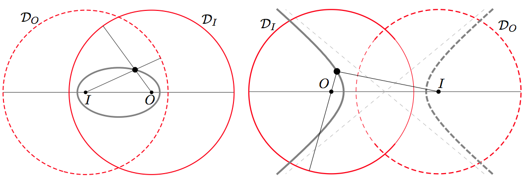
Figure 1: Director circles for ellipses and hyperbolas.

The equivalence of the ‘gardener’ characterisation and the one based in the focus-director circle pair is clear. For ellipses and hyperbolas the two director circles $\mathcal{D}_{O}$ and $\mathcal{D}_{I}$ have its centers at the ‘other’ focus $I$, $O$, and radius equal to the major axis $2a$. A central symmetry in the ellipse or hyperbola centre swaps the two focus and the two director circles. The non-generic type of conics, parabolas, have no centre and the radii of the two director circles, that must be equal, are infinite. In this case, (i) the focus $I$ goes to infinity, and with it the director circle $\mathcal{D}_{I}$ (with centre at $O$) goes also to infinity; and (ii) the director circle $\mathcal{D}_{O}$ has centre at infinity, and appears as a straight line, which is the parabola directrix $D$.

Another basic property of Euclidean circles should be mentioned. Let a circle $\mathcal{C}$ and a fixed point $P$ be given in the plane. Consider all straight lines in that plane through $P$.

• If $P$ is interior to $\mathcal{C}$ all these lines will intersect $\mathcal{C}$ in two (real) points.

• If the point $P$ is exterior to $\mathcal{C}$, then there will be two real tangent straight lines to $\mathcal{C}$ through $P$, and all straight lines within the wedge limited by the two tangents will intersect $\mathcal{C}$ in two real points.

In all these cases, if $d_{1}$ and $d_{2}$ denote the (oriented) distances from $P$ to the two intersection points along a particular straight line, then the product $d_{1}d_{2}$ turns out to be independent of the chosen straight line. This value is called the ‘power of the point $P$ relative to the circle $\mathcal{C}$. This power is negative if the point $P$ is inside $\mathcal{C}$ (then $d_{1},d_{2}$ have opposite orientations) and is positive if $P$ is outside $\mathcal{C}$. A proof is easily constructed and we leave it to the reader.

2.2 Some non-standard 2d vector calculus

In a 2D plane, there is a canonical way to associate to any vector ${\bf w}$ another vector denoted ${}^{*}{}{\bf w}$ (to be understood as a single symbol). This possibility is specific for a 2D plane and does not happen in the 3D space, where the ‘similar’ construction, the vector product, requires to start from two vectors. The vector ${}^{*}{}{\bf w}$ is defined to be the (unique) vector in this plane orthogonal to ${\bf w}$, with the same modulus as ${\bf w}$ and such that the pair $({\bf w},{}^{*}{}{\bf w})$ is positively oriented. The vector ${}^{*}{}{\bf w}$ is obtained from ${\bf w}$ by a rotation in the plane by an angle $+\pi/2$, and component-wise, ${}^{*}{}w_{j}=\epsilon_{ij}w^{i}$ (with sum in the repeated index $i$), i.e., if ${\bf w}=(w^{1},w^{2})$, then ${}^{*}{\bf w}=(-w^{2},w^{1})$. We now state two properties which are easy to check:

• ${}^{*}{}({}^{*}{}{\bf w})=-{\bf w}$.

• If ${\bf L}$ is a vector perpendicular to this plane, then the vector product ${\bf L}\times{\bf w}$ can be expressed in terms of the modulus $L$ of ${\bf L}$ and of ${}^{*}{}{\bf w}$, as ${\bf L}\times{\bf w}={L\,}^{*}{\bf w}$.

In the natural identification $(x,y)\equiv x+{\rm i}\,y$ of the Euclidean plane ${\mathbb{R}}^{2}$ with ${\mathbb{C}}$, the operator ${\bf w}\to{}^{*}{\bf w}$ corresponds to multiplication by the complex unit ${\rm i}$.

3 The geometric approach to the Kepler first law

3.1 Feynman approach for elliptic orbits

In 1964, Feynman delivered a lecture on ‘The motion of planets around the sun’ which was not included in the published ‘Lectures on Physics’. Feynman’s notes for this lecture were eventually found, and then published and commented by Goodstein and Goodstein in 1996 [16]. In his peculiar style, Feynman gave an elementary derivation of Kepler first law by focussing attention in the hodograph. Such derivation starts by unveiling (rediscovering) a curious property: the Kepler hodographs have an exact circular character, but this circle is not centred in the origin of velocity space (see e.g. [17, 18, 19, 20, 21, 22, 23]).

The publication of the ‘Lost Lecture’ has made this approach to the Kepler problem more widely known than before, although, as Counihan points out in [24], this geometric approach was probably more in line with the background of XIX century mathematical physicists than it is nowadays.

This procedure of studying the Kepler motion reduces to a minimum the resort to calculus or to differential equations. All the ‘hodograph first’ approaches to solve Kepler problem (Feynman’s included) require to establish first the circular nature of the Kepler hodograph. Some resort—more or less concealed— to solving a differential equation is required here. The standard way is to write the Newton laws for the motion ${\bf x}(t)$ in a central field of forces with an $1/r^{2}$ radial dependence and look for the differential equation satisfied for the velocity $\dot{\bf x}(t)$ (see e.g. Milnor [25], where one can find a careful discussion).

Newton had to solve this problem by a geometrical argument involving a kind of discretisation of the problem, considering positions at equispaced times $t,t+\Delta t,t+2\Delta t,\dots$, and, as it is well known, this leads to a complicated description.

But since Hamilton we know that this non-linear problem can be transformed to a linear one if we change the time $t$ by the angle $\phi$ as the independent variable and we then enforce the law of areas. The function $\dot{\bf x}(\phi)$ which gives the velocity in terms of the angle $\phi$ satisfies a linear equation whose solutions are immediately seen to be circles in the velocity space. Feynman solved this step by making a kind of discretisation similar to the one by Newton, but involving equispaced angular positions $\phi,\phi+\Delta\phi,\phi+2\Delta\phi,\dots$ on the orbit. This provides some kind of discrete analogous of the linear equation satisfied by $\dot{\bf x}(\phi)$, and leads in the limit $\Delta\phi\to 0$ to the circular character of the hodograph. Once this fact has been established, Kepler first law follows in a simple and purely algebraic way.

Of course, it remains to describe the relation among the hodograph and the orbit. We need a construction which applied to the hodograph would allow us to recover the orbit. In the Feynman lecture, even if rather informally presented, this is accomplished through a sequence of three transformations, whose essential part is to rotate the hodograph by $-\pi/2$ around the origin $O$. All the necessary details will be given in the following sections, after dealing with another recent construction, due to van Haandel and Heckman.

3.2 van Haandel–Heckman approach for elliptic orbits

Van Haandel and Heckman [9] introduced a modification in the Feynman approach which reverses the standard ‘hodograph approach’, and even avoids the need to draw on a differential equation, thus providing a good way to present the problem to beginners. They compare their derivation with the one devised by Feynman and put both into perspective against the original Newton derivation. This comparison makes sense because all three derivations are framed in the language of synthetical Euclidean geometry.

The geometric construction they propose has many elements in common with the previous ones (Maxwell, Feynman, …) but they look at the problem from a different perspective which leads much more directly to two essential insights in the problem: the conic nature of the orbits and the existence of an ‘exceptional’ Keplerian constant of motion ${\bf I}$. It is worth to emphasise that the derivation is purely algebraic, and at no stage a resort to a differential equation should be done (in contrast to Feynman approach).

The standard Laplace-Runge-Lenz (LRL) vector ${\bf A}$ is known to point from the force centre to the perihelion, along the orbit major axis, with modulus $k\,e$; otherwise ${\bf A}$ lacks any geometrical interpretation. On the contrary, the constant vector ${\bf I}$ which follows from this approach is a a rescaling of the standard LRL vector ${\bf A}$ by a factor $1/E$, ${\bf I}={\bf A}/{E}$ and admits a nice and direct geometrical interpretation: both for elliptic and hyperbolic orbits it goes from the force centre, which is one focus of the orbit, to the ‘second’ or ‘empty’ focus (it degenerates to an infinite modulus vector along the conic axis for parabolic orbits).

We start by recalling the elementary proof of Kepler first law as proposed by Van Haandel and Heckman in [9]. Consider Kepler orbits with $L\neq 0$ and $E<0$ (we already know they are Kepler ellipses, but assume at this point that we do not know this).

As a consequence of energy conservation, motion in configuration space (or in the plane of motion) is confined to the interior of a circle ${\mathcal{D}}$, centred at the origin and with radius $k/(-E)$. Outside this circle the kinetical energy would be negative, and thus this exterior region is forbidden for classical motion. This circle $\mathcal{D}$ plays an important role (but as we shall see later, this role is not exactly as the boundary of energetically allowed region, though this is the way van Haandel–Heckman presented the construction).

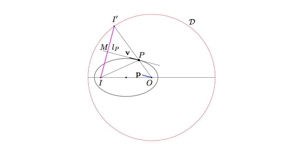
Figure 2: The van Haandel-Heckman construction: $E<0$ Kepler orbits are ellipses

Let be ${\bf r}$ the position vector of a point $P$ on a given orbit, $l_{P}$ denote the tangent line to the orbit at $P$, ${\bf v}$ the velocity of the particle at $P$ and ${\bf p}$ the linear momentum vector, which we will imagine as attached to the origin $O$, i.e., the vector ${\bf p}$ is the result of transporting the vector $m{\bf v}$ to the origin $O$ (recall we are assuming $m=1$).

The geometric construction will proceed in two steps.

1. First, extend the radius vector $OP\equiv{\bf r}$ of $P$ (with the potential centre $O$ as origin) until it meets the circle $\mathcal{D}$ at $I^{\prime}$. This can be seen as the result of scaling by a factor $({k}/{-E})({1}/{r})$, which sends the vector $OP\equiv{\bf r}$ to a new vector with a modulus equal to $({k}/{-E})({1}/{r})r=({k}/{-E})$, so this vector tip $I^{\prime}$ lies on the circle $\mathcal{D}$.

2. Now consider the image $I$ of $I^{\prime}$ under reflection with respect to the line $l_{P}$.

This construction could be done for any bounded $E<0$ motion in any bounding arbitrary central potential; as $P$ moves along the orbit, the point $I^{\prime}$ moves on $\mathcal{D}$ and one might expect the point $I$ to move as well. This is the case for motions in other central fields, but Kepler motion is exceptional in this respect, and we have the following result:

Theorem 1

When $P$ moves along a $E<0$ Kepler orbit and the point $I^{\prime}$ determined by the previous construction moves on the circle $\mathcal{D}$, then the point $I$ stays fixed.

In other words, $I$ turns out to be independent of the choice of the point $P$ on the orbit. As we shall see, this geometric ‘timeless’ construction, displayed in Figure 2, will reflect the existence of a constant of motion specific to the Kepler potential.

Before sketching the proof of the Theorem itself, notice that in the figure, the Kepler orbit has been already displayed as an ellipse. Actually, the elliptic nature of the orbits immediately follows as a consequence of the previous theorem:

Corollary 1

(Kepler first law for elliptic orbits). The Kepler orbit with total energy $E<0$ is an ellipse, with a focus at the origin $O$, the other focus at $I$, and major axis $2a$ equal to the radius $k/(-E)$ of the circle $\mathcal{D}$.

Proof: $OP$ and $PI^{\prime}$ are on the same line, hence $|OP|+|PI^{\prime}|=k/(-E)$. The reflection in the line $l_{P}$ is an Euclidean isometry, so $|PI|=|PI^{\prime}|$, and then $|OP|+|PI|=k/(-E)$, so the sum of distances from $P$ to the fixed points $O$ and $I$ do not change when $P$ moves on the orbit, and it is equal to the radius of the circle $\mathcal{D}$. This agrees with the ‘gardener’ geometric definition of an ellipse with foci $O$ and $I$.

We return to the proof of the theorem which boils down to two stages:

1. Express the vector ${\bf I}\equiv OI$ in terms of the instantaneous state variables of the particle at $P$ (i.e., position ${\bf r}$ and velocity ${\bf v}$ or momentum ${\bf p}$).

2. Compute its time derivative and use the Newton’s equations for the Kepler potential to check that ${\bf I}$ is indeed a constant of motion.

As ${\bf I}=OI=OI^{\prime}-II^{\prime}$, the first step can be carried out by evaluating the vectors $OI^{\prime}$ and $II^{\prime}$. $I^{\prime}$ lies on the circle $\mathcal{D}$ and then $OI^{\prime}=\frac{k}{-E}\frac{{\bf r}}{r}$, which immediately leads to

$$PI^{\prime}=OI^{\prime}-OP=\frac{k}{-E}\frac{{\bf r}}{r}-{\bf r}=\left(\frac{k}{-E}\frac{1}{r}-1\right){\bf r},$$ (2)

and using that by conservation of energy we have $E=\frac{p^{2}}{2}-\frac{k}{r}$, we get

$$PI^{\prime}=\frac{p^{2}}{-2E}{\bf r}.$$ (3)

Now, to compute $II^{\prime}$, we first note that ${\bf p}\times{\bf L}/pL$ is a unit vector perpendicular to both ${\bf p}$ and ${\bf L}$ (which are also mutually perpendicular), so it has the direction of $II^{\prime}$. The length $MI^{\prime}$ is the projection of the vector $PI^{\prime}$ over the line $II^{\prime}$, and it can be computed as the scalar product $\frac{{\bf p}\times{\bf L}}{pL}\cdot\frac{p^{2}}{-2E}{\bf r}$. By using the cyclic symmetry of triple product, we get ${\bf p}\times{\bf L}\cdot{\bf r}={\bf r}\times{\bf p}\cdot{\bf L}={\bf L}^{2}=L^{2}$, and hence we finally have for $II^{\prime}$ and I

$$II^{\prime}=\frac{{\bf p}\times{\bf L}}{-E}=\frac{L}{E}{}^{*}{\bf p},\qquad{\bf I}=\frac{k}{-E}\frac{{\bf r}}{r}-\frac{{\bf p}\times{\bf L}}{-E}.$$ (4)

In order to check that ${\bf I}$ is actually a constant of motion we can introduce

$${\bf A}:=E\,{\bf I}={\bf p}\times{\bf L}-k\frac{{\bf r}}{r},$$ (5)

and as $E$ itself is a constant of motion, the second step reduces to checking that ${\bf A}$ is also a constant of motion for the Kepler potential. Note that $\dot{\bf L}=0$ and that $\dot{\bf p}={\bf F}$, then,

$${\frac{d}{dt}{\bf A}}={\bf F}\times{\bf L}-k\frac{d}{dt}{\left(\frac{{\bf r}}{r}\right)}$$ (6)

with ${\bf F}({\bf r})=-(k/r^{2})(\frac{{\bf r}}{r})$ and a simple direct computation leads to ${\dot{\bf A}}={\bf 0}$. Of course, ${\bf A}$ is but the standard Laplace-Runge-Lenz vector, the specific Kepler constant of motion.

As stressed by vHH, one merit of this approach is that the specifically Keplerian constant of motion follows directly from the construction, so the only remaining task is to check it is a constant, which is the easy part; on the contrary, in the standard approaches, it is not so obvious to figure out the expression which turn out to be a constant of motion.

A direct consequence follows from formula (4): as ${\bf p}$ and ${\bf L}$ are perpendicular, we have for the modulus of the affine vector $II^{\prime}$ the relation $|II^{\prime}|=\frac{L}{-E}\,p$, (notice that $L$ and $-E$ are both positive). This relation, which will be essential for the relation among orbits and hodographs, can be stated as follows:

Proposition 1

For Kepler orbits with $E<0$, as $P$ moves along the orbit, the Euclidean length $|II^{\prime}|$ is proportional to the modulus of the momentum ${\bf p}$ the particle has when it is at $P$:

$$|II^{\prime}|=\frac{L}{-E}\,p$$ (7)

In terms of the geometry of the ellipse, the minor semiaxis length is $b=L/(2\sqrt{-E})$, so the coefficient $L/(-E)$ in (7) admits an alternative expression as ${L}/({-E})={2b^{2}}/{L}$.

Then we can sum up these results in two different but equivalent ways:

• In the direct construction, for any point $P$ on the Kepler orbit, produce the radius vector once it meets the circle ${\mathcal{D}}$ at $I^{\prime}$ and reflect with respect to the tangent line to the orbit at $P$; the reflected point $I$ does not depend on $P$.

• In the reverse construction, choose any point $I^{\prime}$ on the circle ${\mathcal{D}}$ and consider the bisector line of the segment $II^{\prime}$; this is the tangent to the orbit at some point $P$, and when $I^{\prime}$ moves along ${\mathcal{D}}$, the orbit is recovered as the envelope of the family of its tangent lines; it is an ellipse with major axis length $2a$, which can also be described as the set of points equidistant to the fixed point $O$ and the fixed circle ${\mathcal{D}}$.

We recall that the circle $\mathcal{D}$, was introduced by vHH as the boundary of the energetically allowed region for an orbit with energy $E<0$. But now we see from the previous discussion, that the essential property of this circle is precisely to be a director circle ${\mathcal{D}}_{I}$ of the ellipse [14] (the director circle companion to the focus $I$).

3.3 Hyperbolic orbits

The geometric approach described in the previous subsection was only concerned with elliptic orbits. The main point was the identification of the circle ${\mathcal{D}}$ as the director circle of the orbit. We now extend the approach to the case $E>0$.

Now mimic the previous construction for a hyperbolic Kepler orbit ($L\neq 0$ and $E>0$):

1. First, at a point $P$ on the orbit with tangent line $l_{P}$, scale the radius vector ${\bf r}$ of $P$ by a factor ${k}/{(-E)}\cdot{1}/{r}$, (notice that for $E>0$ this factor is negative). This brings the point $P$ to a new point $I^{\prime}$ which lies on some circle with center $O$ and radius $k/|E|$, still denoted ${\mathcal{D}}$ (now $OI^{\prime}$ has the opposite orientation to $OP$). In other words, extend the vector $OP$ starting from $O$ in the opposite sense to ${\bf r}$ until the rescaled vector ${k}/{(-E)}\cdot{{\bf r}}/{r}$ lies precisely on the circle $\mathcal{D}$ at a point $I^{\prime}$ (see Figure 3).

2. Now consider the image $I$ of $I^{\prime}$ under reflection with respect to the line $l_{P}$.

Now the main result follows:

As $P$ moves on the orbit, the point $I^{\prime}$ moves on the circle $\mathcal{D}$ and the point $I$ stays fixed; from this the hyperbolic nature of the orbit follows.

(To be precise, $I^{\prime}$ moves only on an arc of $\mathcal{D}$, displayed in continuous red; the remaining, not displayed, part of the full circle would correspond to the other hyperbola branch, which would be the orbit for the repulsive Kepler problem). The reflection of $I^{\prime}$ in the tangent line $l_{P}$ gives a point $I$, which is outside the circle $\mathcal{D}_{I}$. The result now is that the point $I$ stays at a fixed position when $P$ runs the whole Kepler orbit.

In other words, even in the cases where $E>0$, the orbit is also a conic (here a hyperbola branch) and the circle $\mathcal{D}$ is a director circle of the conic.

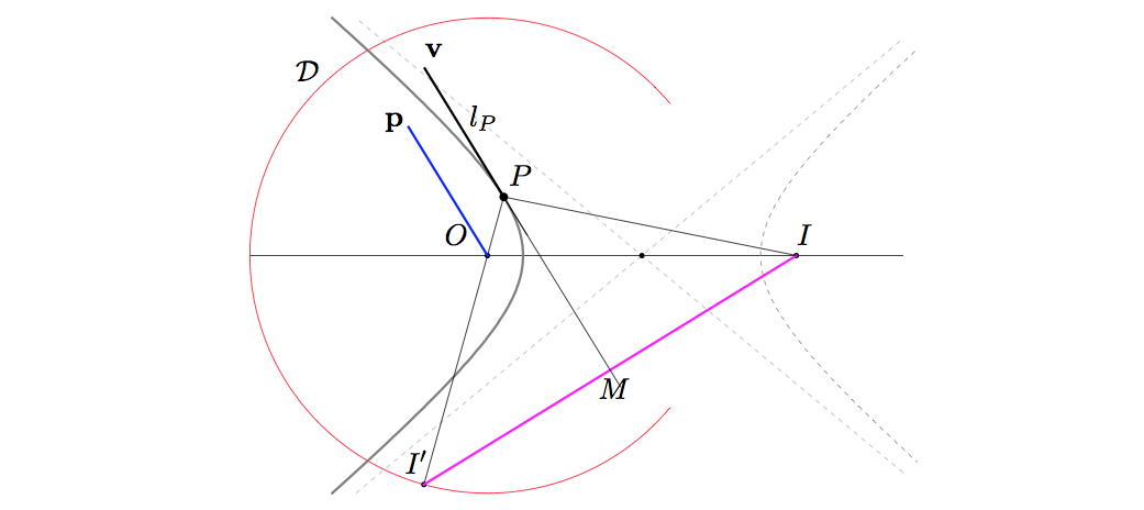
Figure 3: The extension of the van Haandel-Heckman construction to prove that $E>0$ Kepler orbits are hyperbolas.

3.4 Generic orbits

Now we restate the vHH construction in a way which applies at the same time to both elliptic and/or hyperbolic orbits.

Given a Kepler orbit with energy $E\neq 0$, for each point $P$ on the orbit, scale the radius vector of the point $P$ with the factor $({k}/{-E})\cdot({1}/{r})$, and call $I^{\prime}$ the point so obtained, which lies on the circle $\mathcal{D}$ with centre $O$ and radius ${k}/{|E|}$. Now consider the image $I$ of $I^{\prime}$ under reflection in the line $l_{P}$ which is the tangent to the orbit at $P$. What singles out the Kepler motion in either the negative or the positive energy regimes is the following result:

Theorem 2

When $P$ travels along a Kepler orbit with $E\neq 0$ under the Kepler central potential $V(r)=-k/r$, and the point $I^{\prime}$ moves while lying on the circle ${\mathcal{D}}$ (whose centre is $O$ and whose radius is $k/|E|$), then the point $I$ stays at a fixed position.

To check that ${\bf I}$ is indeed a constant of motion for any non-zero energy $E$ requires a computation which exactly mimic the one performed in the elliptic case. Now for both elliptic and hyperbolic orbits, the relation between the constant vector ${\bf I}$ which appears naturally in this approach and the standard Laplace-Runge-Lenz vector ${\bf A}$ is ${\bf I}={\bf A}/{E}$.

The reflection with respect to the line $l_{P}$ is an Euclidean isometry and therefore, $|PI|=|PI^{\prime}|$, while $PO$ and $PI^{\prime}$ are on the same line by construction, but in the present $E>0$ case there is a slight difference with the previous case: the segment $PO$ is fully contained in $PI^{\prime}$, instead of being two adjacent disjoint segments, so that along a positive energy orbit, $|OI^{\prime}|=|PI^{\prime}|-|PO|=|PI|-|PO|$ is a constant length, more precisely equal to the radius $2a=k/|E|$ of the circle $\mathcal{D}$; in this case the quantity which is constant along the Kepler orbit is not the sum but the difference of the distances from a generic point on the orbit $P$ to the two fixed points $O$ and $I$, and that condition is one of the classical geometric definitions of a hyperbola. We have got:

Corollary 2

(Kepler first law for elliptic and hyperbolic orbits) An $E\neq 0$ Kepler orbit is either an ellipse or a branch of a hyperbola, with a focus at the origin $O$ and major axis $2a=k/|E|$. The ‘other’ focus $I$ is inside the circle $\mathcal{D}$ of radius $2a$ for $E<0$ and outside $\mathcal{D}$ for $E>0$.

Proposition 2

As $P$ moves along an $E\neq 0$ Kepler orbit, the Euclidean length $|I^{\prime}I|$ is proportional to the modulus of the linear momentum ${\bf p}$ at $P$:

$$|II^{\prime}|=\frac{L}{|E|}\,p=\frac{2b^{2}}{L}\,p.$$ (8)

Here $b$ refers to minor axis length of the conic. The proof is identical to that of the case $E<0$ with very minor changes: for instance $OM$ and $IN$ lie on different sides to the tangent, so here with $\rho_{I}:=IM,\ \rho_{O}:=ON$ we have $\rho_{I}\rho_{O}=-b^{2}$ ($b$ is the hyperbola minor semiaxis length) independently of the choice of the tangent (or of the point $P$).

The Laplace-Runge-Lenz vector ${\bf A}$ is a vector at $O$ which points towards the periastron, with modulus $A=k\,e$ ($e$ being the eccentricity). This is so for all the signs of the energy (recall $0<e<1$ for negative energy or $e>1$ for positive energy). If now we translate this to the new constant ${\bf I}=\bf A/{E}$, we have to discuss the two different generic situations according as $E<0$ or $E>0$.

• In the $E<0$ case, as $E=-k/(2a)$, the vector ${\bf I}$ points towards the apoastron, and its modulus is $ke/(k/2a)=2ae=2f$, so this computation confirms the result stated earlier: the tip of ${\bf I}$ lies at the ellipse ‘empty’ focus which lie inside $\mathcal{D}$ as $e<1$.

• In the hyperbolic case, as $E=k/(2a)$, the vector ${\bf I}$ points towards the periastron, and its modulus is again given by $ke/(k/2a)=2ae=2f$, so as stated before the tip of ${\bf I}$ lies at the hyperbola ‘empty’ focus, which, as $e>1$, lies outside the circle $\mathcal{D}$.

Hence, in all cases, the constant vector ${\bf I}$ points from the origin to the empty focus (and of course, for the parabolic orbits, the modulus of ${\bf I}$ goes to infinity). The essential role the circle $\mathcal{D}$ plays in this construction is not to be the boundary of the energetically allowed region (which for orbits with $E>0$ would be the whole space) but instead to be a director circle ${\mathcal{D}}_{I}$ for the conic. We can sum up the results:

Theorem 3

(Circular character of the Kepler hodograph, [1]) The hodograph ${\mathcal{H}}$ of any Kepler motion is a circle in ‘momentum space’, centred at the point ${}^{*}{\!}{\bf A}/L$ and radius $k/L$.

We give a proof within the vHH line of argument. When $E\neq 0$, constancy of the vector

$${\bf I}=\frac{k}{-E}\frac{{\bf r}}{r}-\frac{L{}^{*}{\bf p}}{-E}=\frac{1}{E}{\bf A}$$

implies

$$-{}^{*}{\bf p}=\frac{\bf A}{L}+\frac{k}{L}\frac{{\bf r}}{r}\qquad\text{and}\qquad{\bf p}={}^{*}(-{}^{*}{\bf p})=\frac{{}^{*}\bf A}{L}+\frac{k}{L}\frac{{{}^{*}\bf r}}{r}.$$

When $P$ (i.e., ${\bf r}$) moves along the Kepler orbit, this is the equation of a circle in the ${\bf p}$ space, with centre and radius as stated.

The ‘offset’ in momentum space between the centre of ${\mathcal{H}}$ and the origin point ${\bf p}={\bf 0}$ is ${|{}^{*}\bf A|}/{L}=k\,e/L$ and for this reason the vector ${}^{*}{\!}{\bf A}$ is called the ‘eccentricity vector’, because the centre is offset from the origin by a fraction $e$ of the hodograph radius. The linear momentum space origin $O\equiv{\bf p}={\bf 0}$ is thus inside ${\mathcal{H}}$ for $E<0$ and outside ${\mathcal{H}}$ for $E>0$; in the latter case the actual hodograph is not the complete circle but only the arc of ${\mathcal{H}}$ lying in the region ${\bf p}^{2}>2E$: in a hyperbolic motion the modulus of the momentum is always larger than the modulus of the linear momentum when the particle is ‘at infinity’.

This important result follows from the geometric construction, and the proof underlines the close connection between constancy of ${\bf A}$ and circular character of the hodographs.

The standard proof, dating back to Hamilton (see e.g. [25]) derives this property from a differential equation obtained from Newton laws by changing the time parameter $t$ to the polar angle $\phi$. We have shown that even this step can be dispensed with, as in the vHH approach this circular character of hodographs follows from the fact that ${\bf I}$ is actually a constant of motion. Actually, this result requires to use the Newton’s equations of motion, so the result does not come from nothing; the point to be stressed is that we must use directly Newton’s equations, but we can completely bypass solving them in any form.

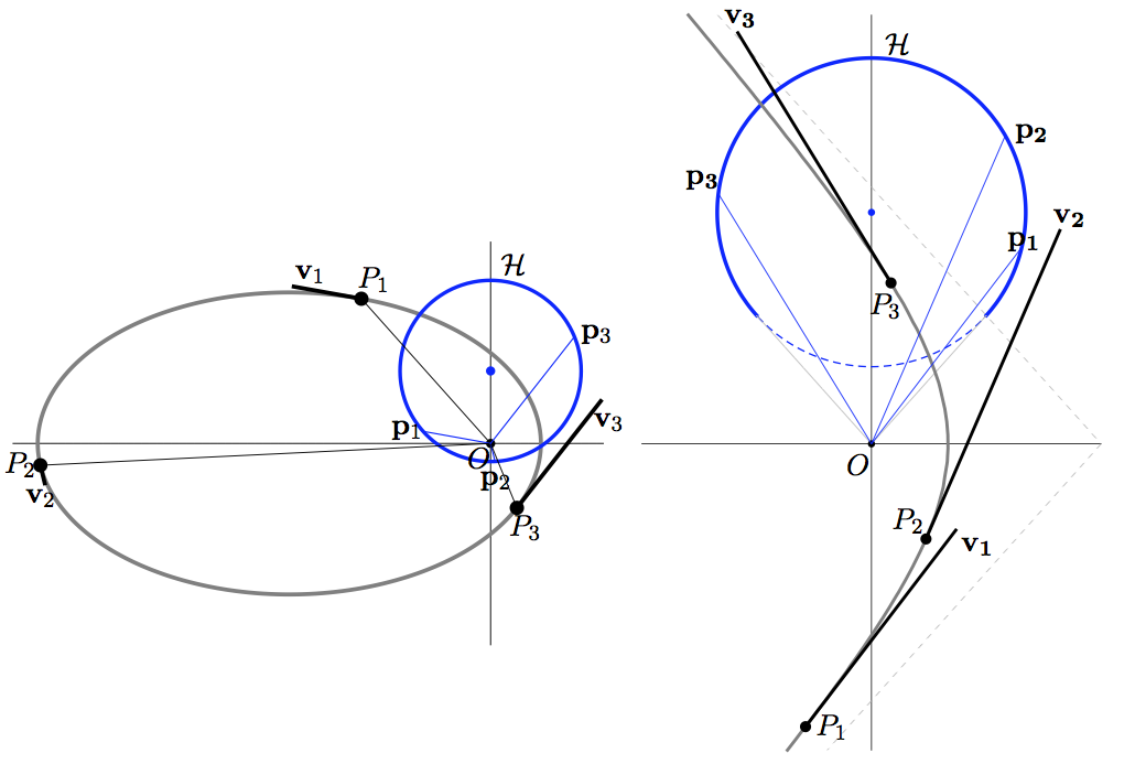
Figure 4: The hodograph for elliptic $E<0$ and hyperbolic $E>0$ Kepler orbits.

3.5 Parabolic orbits

The $E=0$ parabolic case may be reached as a limit $E\to 0$ from negative or from positive $E$ values. In both situations, $\mathcal{D}$ tends to a circle with centre at $O$ and infinite radius. Thus the original vHH construction degenerates for $E=0$ unless a suitable modification is done which allows to deal with this limit in a regular way. One can make a natural choice for this radius so that in the parabolic case we get also a working construction (this is described e.g., in the Derbes paper [2]; we will not discuss here this question any longer).

As the energy $E$ itself disappears from the hodograph equation (which depends only on ${\bf A}$ and $L$), the result whose proof has been given for $E\neq 0$ remains also valid for parabolic orbits. In the $E=0$ parabolic case the hodograph passes through the origin.

4 Streamlining the geometric construction

Now we propose a variant of the vHH construction which at the end will simplify it. This reformulation turns out to be equivalent to the previous one for the Euclidean Kepler problem. But this reformulation has some additional interest, because it allows a direct extension for the ‘curved’ Kepler problem in a configuration space of constant curvature, either a sphere or a hyperbolic plane [8, 10, 26].

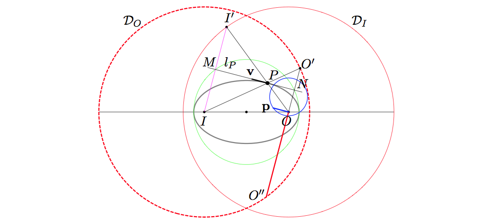
Figure 5: The ‘complete’ constructions for elliptic $E<0$, Kepler orbits.

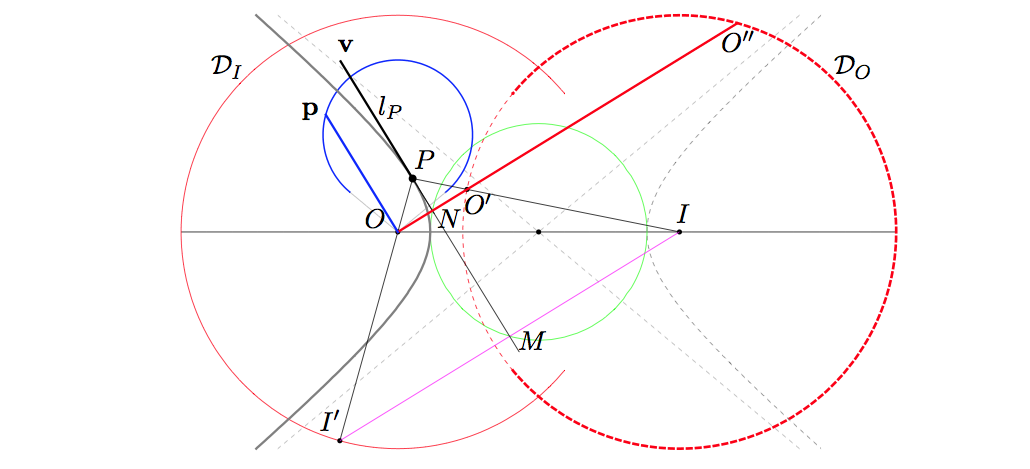
Figure 6: The ‘complete’ constructions for hyperbolic $E>0$ Kepler orbits.

The conics obtained as orbits have not just one pair of matching ‘director circle – focus point’ but actually two pairs. Further to the director circle $\mathcal{D}\equiv{\mathcal{D}}_{I}$ associated to the focus $I$ (which is the only director circle considered up to now), there is also another director circle ${\mathcal{D}}_{O}$, ‘matching’ to the focus $O$ and such that the conic is also the set of points equidistant from ${\mathcal{D}}_{O}$ and $O$. ${\mathcal{D}}_{O}$ can be obtained from ${\mathcal{D}}_{I}$ by a central reflection with respect to the conic centre, and thus ${\mathcal{D}}_{O}$ is a circle centred at $I$ and with radius $2a=k/|E|$. In the figures where both director circles are displayed, the circle ${\mathcal{D}}_{O}$ is dashed.

Once we know that the generic $E\neq 0$ Kepler orbits are ellipses or hyperbolas, the previously described construction can be extended by considering the central reflection with respect to the centre of the conic. This maps the director circle ${\mathcal{D}}_{O}$ onto ${\mathcal{D}}_{I}$. The image of $II^{\prime}$ under this central reflection is $OO^{\prime\prime}$, where $O^{\prime\prime}$ is the second intersection point of the line $OO^{\prime}$ with $\mathcal{D}_{O}$. As a consequence of this relation, we may state:

Theorem 4

When $P$ travels along a $E\neq 0$ Kepler orbit under the Kepler central potential $V(r)=-k/r$, then the point $O^{\prime\prime}$ lies on the director circle ${\mathcal{D}}_{O}$ (whose centre is $I$), and the Euclidean length $|OO^{\prime\prime}|$ is proportional to the modulus $p$ of the linear momentum ${\bf p}$:

$$|OO^{\prime\prime}|=\frac{2b^{2}}{L}p=\frac{L}{|E|}p$$ (9)

This result is displayed in Figures 5 and 6, where $II^{\prime}$ is shown in magenta and its image $OO^{\prime\prime}$ under the central reflection, in red. Seen as affine vectors, $II^{\prime}=-OO^{\prime\prime}$ and $IO^{\prime\prime}=-OI^{\prime}$. The orbit is in dark grey, the director circles in red and dashed red, and the hodograph and the momentum vector are in blue. In all cases $II^{\prime}$ and $OO^{\prime\prime}$ are related by a central reflection with respect to the conic centre and their equal lengths are proportional to the modulus of the linear momentum ${\bf p}$. $II^{\prime}$ is orthogonal to the tangent line $l_{P}$ while $OO^{\prime\prime}$ is perpendicular to the linear momentum vector ${\bf p}$.

4.1 Relation with the hodograph

The next interesting question is to describe the relation between the hodograph and the orbit. Starting from the circular character of the hodograph, we need a construction which applied to the hodograph (whose circular nature is appealing) would allow us to recover the orbit. We mentioned how Feynman did this in a rather descriptive and informal way. But now, using the setting provided by the vHH construction, we can describe precisely what Feynman did with full detail through a sequence of three transformations:

1. A rotation by $-\pi/2$ around the origin $O$,

2. A homothety around the origin with a scale factor $L/(-E)$ and finally

3. A translation by a vector ${\bf I}$.

This sequence of transformations can be shown to apply the hodograph ${\mathcal{H}}$ to the director circle $\mathcal{D}$ and the linear momentum vector ${\bf p}$ to the vector $II^{\prime}$.

We can see that the reformulation of the previous section, which related $E\neq 0$ Kepler motions along the orbit with those of an auxiliary point $O^{\prime\prime}$ on the director circle ${\mathcal{D}}_{O}$, allows us to describe this relationship in a simpler way. The important elements in this construction are the rotation by a quarter of a turn, as used by Feynman [16] (but note the opposite sign), and then a homothety; the ‘translation’ step appearing in the Feynman lecture is no longer required, and the two remaining (and now commuting) steps are enough to relate the hodograph to the director circle and then to the orbit.

Theorem 5

(Relation of Kepler hodograph with the configuration space orbit) The sequence of the two following transformations

1. Rotation by $+\pi/2$ around the origin $O$,

2. Homotethy around the origin with a scale factor $L/(-E)$,

applies the hodograph ${\mathcal{H}}$ to the director circle ${\mathcal{D}}_{O}$ and the linear momentum vector ${\bf p}$ on the vector $OO^{\prime\prime}$. The Kepler orbit corresponding to the hodograph ${\mathcal{H}}$ is the envelope of the perpendicular bisectors of the vectors $OO^{\prime}$ when $O^{\prime}$ moves along the director circle ${\mathcal{D}}_{O}$. Or, alternatively, the Kepler orbit is the locus of points in configuration space which are equidistant from the origin $O$ and from the director circle ${\mathcal{D}}_{O}$.

Before giving the proof, it is worth insisting that the vHH and the Feynman approaches allowed us to describe the configuration space orbit as the envelope of a family of lines, which were the bisectors of the segments $II^{\prime}$, as the point $I^{\prime}$ moves along the director circle $\mathcal{D}\equiv{\mathcal{D}}_{I}$. But the new reformulation, while keeping a similar property (the configuration space orbit is the envelope of the family of the bisectors of the segments $OO^{\prime}$, as the point $O^{\prime}$ moves along the director circle ${\mathcal{D}}_{O}$) allows us a more direct description of the configuration space orbit: it is the set of points in configuration space which are equidistant from the fixed point $O$ (the centre of forces) and from the fixed circle ${\mathcal{D}}_{O}$.

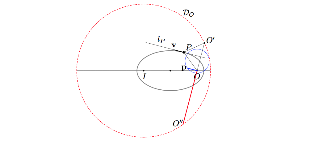
Figure 7: The ‘minimal’ constructions for elliptic $E<0$ Kepler orbits.

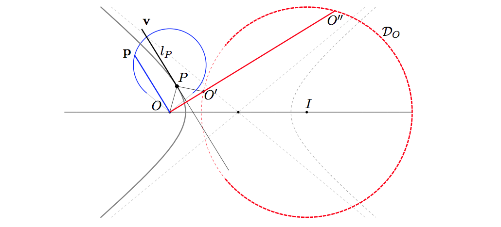
Figure 8: The ‘minimal’ constructions for hyperbolic $E>0$ Kepler orbits.

The proposition follows by direct computation: for any vector ${\bf w}$ in momentum plane, the two steps make the transformations:

$${\bf w}\longmapsto{}^{*}{\bf w}\longmapsto\frac{L}{-E}\,{}^{*}{\bf w}.$$ (10)

Under the composition of the two steps, a generic point on the hodograph ${\bf p}$ goes to

$${\bf p}\longmapsto{}^{*}{\bf p}\longmapsto\frac{L}{-E}\,{}^{*}{\bf p}=\frac{\bf A}{E}-\frac{k}{|E|}\frac{\bf r}{r}\equiv OO^{\prime}.$$ (11)

Notice that $OO^{\prime\prime}$ is automatically perpendicular to ${\bf p}$; the hodograph centre ${}^{*}{\!}{\bf A}/L$ goes to

$$\frac{1}{L}\,{}^{*}{\!\bf A}\longmapsto-\frac{1}{L}{\bf A}\longmapsto\frac{1}{E}{\bf A},$$ (12)

which means that under the two steps the hodograph becomes the director circle ${\mathcal{D}}_{O}$, with radius ${k}/{|E|}$ and centre at $I$. The origin of the linear momentum space, ${\bf p}={\bf 0}$, stays fixed.

This is depicted in Figures 7 and 8, where the director circle ${\mathcal{D}}_{I}$ and all their associate elements have been removed because they are not actually relevant for this streamlined construction. The orbit itself is in dark grey, the director circle $\mathcal{D}_{O}$ in dashed red, and the hodograph and the linear momentum vector are in blue. The relation between the director circle ${\mathcal{D}}_{O}$ and the hodograph, by a rotation of $\pi/2$ and a scaling with factor $L/(-E)$ is clearly displayed; the sign of this scaling factor depends on the sign of the energy.

This sequence of transformations can be shown to apply the hodograph ${\mathcal{H}}$ to the director circle $\mathcal{D}$ and the momentum ${\bf p}$ to the vector $II^{\prime}$. We now see that the reformulation of the previous section, which related $E\neq 0$ Kepler motions along the orbit with those of auxiliary points $O^{\prime\prime}$ on the director circle ${\mathcal{D}}_{O}$, allows us to describe this relationship in an even simpler way. The ‘translation’ step of Feynman lecture is no longer required, and the two remaining (and now commuting) steps are enough to relate the hodograph to the director circle and then to the orbit. The relevant elements in this construction are the rotation by a quarter of a turn, as used by Feynman [16], and then a homothety.

The translation iii) in the Feynman relation among hodograph and orbit only serves to map the director circle ${\mathcal{D}}_{O}$ onto ${\mathcal{D}}_{I}$, and thus it is unnecessary. The ‘correct’ relation among both director circles, swaping ${\mathcal{D}}_{O}$ for ${\mathcal{D}}_{I}$ and $OO^{\prime\prime}$ for $II^{\prime}$ is not actually a translation, but a central reflection with respect to the ellipse or hyperbola centre. As this can be suitably decomposed as a product of a central reflection with respect to $O$ and a translation with vector $OI$, this is the reason for the opposite signs at stage 1) of Theorem 5, as compared with the sign of the rotation angle $-\pi/2$ in the stage i) of the Feynman lecture.

5 A comment on the Kepler problem on curved spaces

The idea that the Kepler problem (and also the harmonic oscillator) can be correctly defined on constant curvature spaces appears in a book of Riemannian geometry of 1905 by Liebmann [27]; but it was Higgs [28] who studied this system with detail in 1979 (the study of Higgs was limited to a spherical geometry but his approach can be extended, introducing the appropriate changes, to the hyperbolic space). Since then several authors have studied the Kepler problem on curved spaces and have analysed the existence of dynamical symmetries leading to constants of motion that can be considered as the appropriate generalisations of the Euclidean Laplace-Runge-Lenz vector. In addition, it has also been proved, by introducing a modified version of the change $u=1/r$, the existence of a curved version of the well known Binet equation (see [10] and references therein).

At this point it seems natural to ask whether the Kepler problem on curved spaces (of a constant curvature) can be analysed by the use of an approach similar to the one presented in previous sections (that is, without integral calculus or differential equations).

At first sight, the answer seems to be negative. The hodograph (defined starting from the velocity vectors) seems to involve an implicit transport of the velocity vector at each point of the orbit to a common origin $O$. In a flat configuration space, parallel transport is uniquely defined, no matter of which path is followed, and this makes irrelevant the question about ‘where are these vectors applied’, either at each point on the orbit $P$ or in a common origin $O$. Thus, to try to extend a ‘velocity based hodograph approach’ to a constant curvature configuration space might seem pointless, because the result of this transport would depend on the path followed, and hence this ’velocity based hodograph’ itself seems to be not well defined. This is of course true.

But the point to be stressed is that the true hodograph should be based in the momenta ${\bf p}$ rather than in the velocity. Indeed the paralell transport is an inessential element in the construction which is only required if one starts with the velocity and not with the Noether momenta ${\bf P}$, as one should. In the construction presented in the previous paragraphs, the most important vector is ${\bf p}$, which is a vector at $O$ (see Figures 2, 3, 4) and coincides with the Noether moment. As the Euclidean parallel transport is path independent, this vector at $O$ coincides with the parallel transported of $v$ along any path joining $P$ to $O$. But in a space of a constant curvature, while the result of some unqualified parallel transport of the velocity vector to $O$ would be undefined, the components of Noether momenta ${\bf P}$ are still well defined, and they are, alike the components of the the other (conserved) Noether momentum ${\bf L}$, a vector at $O$. Nevertheless if in a constant curvature space everything is written in terms of the associated momenta (which are naturally vectors in an auxiliary space), it turns out that both Theorems 4 and 5 have a direct extension to this case.

Henceforth, the construction we have here described allows a quite direct extension to the case of constant curvature configuration space. This will be discussed elsewhere.

6 Final comments

The Kepler problem is studied in all books of Classical Mechanics and it is solved by making use of integral calculus and differential equations (e.g., Binet equation). Nevertheless the Newton approach presented in the Principia was mainly related with the classical language of Euclidean geometry. This property (that it can be solved by the use of a purely geometric approach) is a specific property of the Kepler problem that distinguish it from all the other problems with central forces. This simplicity is a consequence of the existence of an additional constant of motion which is specifically Keplerian: the Laplace-Runge-Lenz vector. In fact, the circular character of the Kepler hodograph, discovered and studied by Hamilton, is just a consequence of the existence of this additional integral of motion.

In the first part of this paper we have reviewed and compared two geometric approaches to the Kepler problem, which were originally devised for only dealing with elliptic orbits. They are due to Feynman and to van Haandel-Eckman. Both fall into the broad class of ‘hodograph approaches’ but the vHH one somehow reverses the usual logic in a way which avoids the recourse to any differential equation, so making this approach accessible to a wider audience. In particular, the vHH approach leads in a natural and purely algebraic way to the specifically Keplerian constant of motion, the Laplace-Runge-Lenz vector.

Then taking this as starting point, we identify the important geometric role of some circles (director circles) entering into these constructions. First, we show that both approaches can be suitably extended to cover, not only bounded elliptic orbits, but also open hyperbolic ones. And second, by making use of the properties of these director circles, the full analysis is streamlined, so that the final ’minimal’ description of the relationship of the hodograph with the true orbit in configuration space is neater than in the previous ones.

The conic nature of the orbit follows from this approach in a purely algebraic way, and this applies both to elliptic and hyperbolic orbits. In summary, this can be very suitable for beginning students, as the Newton laws are simply used directly, but no explicit solving of any differential equation is required.

References

- [1] W.R. Hamilton, The Hodograph, or a new method of expressing in symbolical language the Newtonian law of attraction, Proceedings Roy. Irish Academy III, 344–353 (1847). Reprinted in Mathematical Papers of Sir William Rowan Hamilton, Vol. II, pp. 287–292, edited by A.W. Conway and A.J. McConnell (Cambridge U.P., Cambridge, 1940).
- [2] D. Derbes, Reinventing the wheel: Hodographic solutions of the Kepler problems, Am. J. Phys. 69, 481–489 (2001).
- [3] A.F. Möbius, Die Elemente der Mechanik des Himmels : auf neuem Wege ohne Hülfe hoöherer Rechnungsarten, Sec. 22, p. 47 (Weidmann Verlag, Leipzig, 1843). Reprinted in A. F. Möbius, Gesammelte Werke Vol. IV, edited by W. Scheibner and F. Klein (S Hirzel Verlag, Leipzig, 1887).
- [4] J. C. Maxwell, Matter and Motion, Sec. 133, pp. 108–109 (Dover, New York, 1952).
- [5] M. Kowen an H. Mathur, On Feynman’s analysis of the geometry of Keplerian orbits, Am. J. Phys. 71, 397–401 (2003).
- [6] H. Goldstein, A note on the prehistory of the Runge-Lenz vector, Am. J. Phys. 43, 737–738 (1975).
- [7] H. Goldstein, More on the prehistory of the Laplace or Runge-Lenz vector, Am. J. Phys. 44, 1123–1124 (1976).
- [8] J.F. Cariñena, M.F. Rañada and M. Santander, Superintegrability on curved spaces, orbits and momentum hodographs: revisiting a classical result by Hamilton, J. Phys. A 40, 13645–13666 (2007).
- [9] M. van Haandel and G. Heckman, Teaching the Kepler laws for freshmen, Math. Intelligencer 31, 40–44 (2009).
- [10] J.F. Cariñena, M.F. Rañada and M. Santander, Central potentials on spaces of constant curvature: the Kepler problem, on the two-dimensional sphere and the hyperbolic plane , J. Math. Phys 46, 052702 (2005).
- [11] M.F. Rañada and M. Santander, A new look to Kepler first law: Euclidean approach with a view to the ’curved’ Kepler problem. In the book: Mathematical Physics and Field Theory, pp 331–342, Prensas Univ. Zaragoza (2009).
- [12] I. Newton, The Principia Mathematica. Translation by I.B. Cohen and A. Wihtman (University of California Press, Berkeley, 1999).
- [13] S. Chandrasekhar, Newton’s Principia for the common reader, 2nd ed. (Oxford Univ. Press, 1997).
- [14] D.M.Y. Sommerville, Analytical conics (Bell, London, 1924).
- [15] D. Pedoe, Geometry and the liberal arts (St. Martin’s Press, New York, 1976).
- [16] D.L. Goodstein and J.R. Goodstein, Feynman’s lost lecture: the motion of planets around the sun (Norton, New York, 1996).
- [17] H.A. Abelson, A. diSessa and L. Rudolph, Velocity space and the geometry of planetary orbits, Am. J. Phys. 43, 579–589 (1975).
- [18] J. Stickforth, Complementary Lagrange Formalism in Classical Mechanics, Am. J. Phys. 46, 71–73 (1978).
- [19] J. Stickforth, Kepler problem in momentum space, Am. J. Phys. 46, 74–75 (1978).
- [20] A. González–Villanueva, E. Guillaumín–España, R.P. Martínez–Romero, H.N. Núñez–Yépez and A.L. Salas–Brito, From circular paths to elliptic orbits: a geometric approach to Kepler’s motion, Eur. J. Phys. 19, 431–438 (1998).
- [21] E.I. Butikov, The velocity hodograph for an arbitrary Keplerian motion, Eur. J. Phys. 21, 1–10 (2000).
- [22] T.A. Apostolatos, Hodograph: A useful geometrical tool for solving some difficult problems in dynamics, Am. J. Phys. 71, 261–266 (2003).
- [23] J. Morehead, Visualizing the extra symmetry of the Kepler problem, Am. J. Phys. 73, 234–239 (2005).
- [24] M. Counihan, Presenting Newtonian gravitation, Eur. J. Phys 28, 1189–1197 (2007).
- [25] J. Milnor, On the geometry of the Kepler orbits, Amer. Math. Monthly 90, 353–365 (1983).
- [26] L. García Gutiérrez and M. Santander, Levi-Civita regularization and geodesic flows for the ’curved’ Kepler problem, arXiv:0707.3810v2 [math.phys] (2007).
- [27] H. Liebmann, Nichteuklidische Geometrie, 1st ed. (Göschen’sch Verlag, Leipzig, 1905); 3rd ed. (De Gruyter, Berlin, 1923). The 3rd ed. is a very revised version of the 1st edition.
- [28] P.W. Higgs, Dynamical symmetries in a spherical geometry I, J. Phys. A 12, 309–323 (1979).