Optimized Markov State Models for Metastable Systems

Abstract

A method is proposed to identify target states that optimize a metastability index amongst a set of trial states and use these target states as milestones (or core sets) to build Markov State Models (MSMs). If the optimized metastability index is small, this automatically guarantees the accuracy of the MSM, in the sense that the transitions between the target milestones is indeed approximately Markovian. The method is simple to implement and use, it does not require that the dynamics on the trial milestones be Markovian, and it also offers the possibility to partition the system’s state-space by assigning every trial milestone to the target milestones it is most likely to visit next and to identify transition state regions. Here the method is tested on the Gly-Ala-Gly peptide, where it shown to correctly identify the expected metastable states in the dihedral angle space of the molecule without a priori information about these states. It is also applied to analyze the folding landscape of the Beta3s mini-protein, where it is shown to identify the folded basin as a connecting hub between an helix-rich region, which is entropically stabilized, and a beta-rich region, which is energetically stabilized and acts as a kinetic trap.

I Introduction

Markov State Models (MSMs) have become an integral part of the toolbox used to analyze the output of molecular dynamics (MD) simulations of complex systems such as proteins and other large biomolecules Schutte et al. (1999); Swope et al. (2004); Chodera et al. (2007); Noe and Fischer (2008); Schütte et al. (2011); Schütte and Sarich (2013); Bowman et al. (2013). They were developed in response to the need to process ever longer MD timeseries data, made either of one long trajectory or very many shorter ones, generated e.g by special-purpose high-performance computers Shaw et al. (2010), high-performance GPUs Stone et al. (2007), or massively parallel simulations Voelz et al. (2010). The basic idea of MSMs is to represent the original dynamics as memoryless jumps between predefined states in the configuration space of the molecular system. Under this Markovian assumption, MD timeseries data can then be processed via inference techniques such as maximum likelihood estimation to calculate the rate matrix between these states. This matrix defines a Markov jump process (MJP), which in turns permits the calculation of interesting kinetic quantities of the system on time scales that may be larger than those reached in the MD simulations: indeed MSMs also permit to recombine short simulations run in parallel to extract long time information about the system.

A recurrent issue in the context of MSMs is how to pick the states on which to map the original dynamics – see Refs. McGibbon et al. (2014); Sultan et al. (2014); Martini et al. (2016) for some recent works in this direction. Indeed this mapping amounts to a drastic coarse-graining of the dynamics, and the jumps between poorly chosen coarse states will not be Markovian in general. This invalidates the basic assumption of MSMs and affect their reliability and accuracy. Fortunately, MD systems typically display metastability and this offers a way around this difficulty. In metastable systems there exists regions that play the role of hubs: after visiting one such hub, the system returns often to it before making a transition to another. This guarantees that transitions between these hubs is indeed approximately Markovian, and metastability has therefore been invoked as they key property to justify MSMs and assess their accuracy (see e.g. [Schütte and Sarich, 2013] and [Bowman et al., 2013] for modern perspectives on the topic that summarizes this viewpoint). What remains mostly open, however, is how to identify these hubs in practice.

In the present paper we aim at addressing this question in the context of milestoning-based MSMs Schütte et al. (2011) that combine the core set method originally introduced in Ref. [Buchete and Hummer, 2008] with the milestoning of the trajectories developed in Refs. [Faradjian and Elber, 2004; Vanden-Eijnden et al., 2008; Vanden-Eijnden and Venturoli, 2009]. Unlike standard MSMs that are based on a full partition of the configuration space of the system into blocks that are used as states Krivov and Karplus (2006); Chodera et al. (2007); Sarich et al. (2010); Beauchamp et al. (2011); Vitalis and Caflisch (2012); Fac̆kovec et al. (2015), milestoning-based MSMs uses non-adjacent core sets as states (the milestones), and assign the MD timeseries to the index of the last such milestone it visited. This maps the original dynamics onto a symbolic dynamics on these indices that is then used as input to build the MSM by maximum likelihood estimation of its transition matrix. In metastable systems, the proper milestones to use should be the hubs mentioned before. Here we propose to identify these hubs among a set of trial milestones via optimization of a metastability index that measures how good the hubs are. The method can be justified within the framework of the potential theoretic approach to metastability developed by Bovier and collaborators Bovier et al. (2002, 2004, 2005). It has the advantage that it can be used even in situations where the dynamics on the trial milestones is non-Markovian. In this sense, it alleviates a difficulty with the standard approach used to build MSMs via clustering of trial states Bowman et al. (2013): This clustering is typically done using spectral analysis of the rate matrix of the chain built on these trial states, which may lead to artifacts since the dynamics on these trial states is non-Markovian in general. The method we propose avoids this difficulty altogether. In addition it avoids the need to introduce a time-lag to process the data, which may be difficult to adjust. As we will see, our method also offers a way to partition the state space of the system by identifying regions made of configurations most likely to reach a given hub, and to identify the members of the transition state ensemble as those trial milestones that have a non-negligible probability to reach more than one target milestone next.

The remainder of this paper is organized as follows. In Sec. II we start by presenting the algorithmic aspects of the method we propose, including how to define the trial milestones (Sec. II.1) and the metastability index (Sec. II.2), how to identify the target milestones that optimize this metastability index (Sec. II.3), and how to build the MSM on these target milestones (Sec. II.4). We also introduce a variety of diagnostic tests that can be used a posteriori to analyze the output of the MSM and use the trial milestones to get additional information about the system’s dynamics (Sec. II.5). A theoretical justification of this algorithm is then given in Sec. III, first in the context of Markov jump processes, which is relevant e.g. if one assumes that the dynamics on the trial milestones is itself Markovian (Sec. III.1), then in the context of systems whose configurational space is continuous, like those encountered in MD simulations, where we cannot expect the dynamics on the trial milestones to be Markovian (Sec. III.2). We also test the method on a simple one-dimensional example with a multiscale energy landscape (Sec. III.3). In Sec. IV we then apply the method to analyze the dynamics of a Gly-Ala-Gly peptide, and in Sec. V we use it to analyze the folding pathways of the Beta3s mini-protein. Concluding remarks are given in Sec. VI. Some technical derivations are relegated to an Appendix.

II Algorithmic aspects

In this section, we outline the algorithm we propose to identify the milestones (or core sets) over which to build an MSM. In a nutshell, this is done by picking among a set of trial milestones a subset of target milestones which minimizes a metastability index – this index is defined so that small values are indicative of Markovianity. The target milestones are taken as states in the MSM, while the trial milestones are used to complement the predictions of this MSM and e.g. partition the system’s configurational space or identify transition state regions in it.

Figure 1: Milestoning procedure. (a): piece of a long trajectory ${\boldsymbol{x}}(t)$ crossing a set of three circular milestones, $S_{1}$, $S_{2}$, and $S_{3}$. (b): the trajectory shown in (a) is mapped onto the index of the last milestone it hit, thereby defining the piecewise constant function $i_{*}(t)$.

II.1 Trial versus target milestones

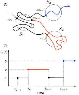
Denote by ${\boldsymbol{x}}(t)\in\mathbb{R}^{3n}$ a trajectory containing the instantaneous position of the $n$ atoms in a molecular system. We assume that we have generated one or several such trajectories and our goal is to build a MSM that captures their main features. To this end, we introduce a set of $N$ trial milestones, which we will denote by $S_{1}$, $S_{2}$, …, $S_{N}$ and label them by their index, i.e. $i$ identifies $S_{i}$. These milestones are disjoint sets in the system’s configuration space that can be defined e.g. by requiring that some of the dihedral angles of the molecules take values between specific bounds, etc. – how to actually choose the trial milestones $S_{i}$ will be illustrated below on specific examples. In the spirit of milestoning, we then map each trajectory ${\boldsymbol{x}}(t)$ onto the index of the last trial milestone $S_{i}$ it hit, see Fig. 1 for an illustration. This way we obtain a piecewise constant index function $i_{*}(t)$ whose value at time $t$ is the index of the last milestone hit by ${\boldsymbol{x}}(t)$. Note in this procedure we discount recrossings: we only update the index function when a new milestone is hit.

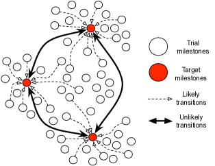
We stress that at this stage we do not assume that the dynamics of the index function $i_{*}(t)$ on the trial milestones is Markov – in general it will not be. What we would like to do next is extract from the set of $N$ trial milestones a subset of $M\leq N$ target milestones such that if we map the trajectory ${\boldsymbol{x}}(t)$ onto this subset of target milestones, the corresponding index function will be approximately Markovian – these target milestones are shown in red in the cartoon shown in Fig. 2. In the sequel, we will denote by $\mathcal{M}=\{i_{1},i_{2},\ldots,i_{M}\}\subset\{1,2,\ldots,N\}$ the set of indices identifying the target milestones, i.e. these are $\{S_{i_{1}},S_{i_{2}},\ldots,S_{i_{M}}\}$. We will also refer to trial milestones that are not target ones as non-target milestones.

II.2 Metastability index

How should the target milestones be chosen? Intuitively, they should be such that they are hubs among the trial milestones towards which the trajectory is attracted but between which it seldom makes transitions, as illustrated in Fig. 2. To make this idea concrete, let us first introduce the probability $\Gamma_{\!i,j}$ that, if the trajectory hits milestone $S_{i}$, then subsequently it will hit $S_{j}$ with $j\not=i$ before hitting $S_{i}$ again (discounting recrossings: recall that only hits of different milestones are counted – in other words, to hit $S_{i}$ again, the trajectory must have hit at least one other milestone in between). To estimate $\Gamma_{\!i,j}$, out of each of the piecewise constant index function $i_{*}(t)$, we first extract the sequence $\{i_{1},i_{2},i_{3},..\}$ of successive values that this function takes – for example, for the timeseries illustrated in Fig. 1 this sequence starts with $i_{1}=1$, $i_{2}=2$, $i_{3}=1$, $i_{4}=3$, etc. We then cut this sequence into the $N_{i}$ pieces which start from $i$ and contain all the indices visited after $i$ before $i$ appears again. For example, if the sequence is made of 3 indices, $i,j,k$, and reads

$$\{i,k,i,j,k,j,i,k,j\},$$ (1)

we cut it into three pieces ($N_{i}=3$)

$$\{i,k\};\quad\{i,j,k,j\};\quad\text{and}\quad\{i,k,j\}$$ (2)

Finally we count the number of pieces $N_{i,j}$ in which $j$ appears at least once (in the example above $N_{i,j}=2$ since $j$ appears in the last two pieces but not in the first), we add up these numbers coming from every piece of $i_{*}(t)$ at our disposal, and we set

$$\hat{\Gamma}_{\!i,j}=\frac{N_{i,j}}{N_{i}}$$ (3)

as estimator for $\Gamma_{i,j}$. Note that the quality of this estimator depends on the lengths of the pieces of timeseries ${\boldsymbol{x}}(t)$ that we have at our disposal, and how to assess the statistical accuracy of (3) is nontrivial. As usual, we cannot expect the estimator to be accurate if these pieces are too short to observe all the relevant events in the dynamics of the system: In the context of (3) this requires that these pieces be long enough that trajectories starting at a non-target milestone have time to reach a target one. Indeed, as we will see below, this condition is sufficient to guarantee that we will correctly identify target from non-target milestones among the trial ones.

We will now use the matrix with entries $\Gamma_{\!i,j}$ to quantify how good a set of target milestones will be to build an MSM. Specifically, given a candidate $\mathcal{M}=\{i_{1},i_{2},\ldots,i_{M}\}$ identifying the target milestones, we estimate the quality of these milestones via their metastability index defined as

$$\rho_{\mathcal{M}}=\frac{\max_{i\in\mathcal{M}}\max_{j\in\mathcal{M}\setminus\{i\}}\Gamma_{\!i,j}}{\min_{i\not\in\mathcal{M}}\max_{j\in\mathcal{M}}\Gamma_{\!i,j}}$$ (4)

The smaller $\rho_{\mathcal{M}}$, the better the set of target milestones identified by $\mathcal{M}=\{i_{1},i_{2},\ldots,i_{M}\}$. This claim will be justified in Sec. III by connecting $\rho_{\mathcal{M}}$ to a quantity originally introduced by Bovier, but let us briefly explain here why it is true. The numerator in (4),

$$\max_{i\in\mathcal{M}}\max_{j\in\mathcal{M}\setminus\{i\}}\Gamma_{\!i,j},$$ (5)

identifies the target milestone $S_{i}$ for which the probability is the highest that, after hitting $S_{i}$, the trajectory will hit some other target milestone $S_{j}$ before hitting $S_{i}$ again. In this sense, $S_{i}$ is the worst target milestone in the set since we would like that transitions between these target milestones be unlikely, and the smaller (5) the better. Correspondingly, the denominator in (4),

$$\min_{i\not\in\mathcal{M}}\max_{j\in\mathcal{M}}\Gamma_{\!i,j},$$ (6)

identifies the non-target milestone $S_{i}$ which is such that the trajectory has the lowest probability to hit a target milestone $S_{j}$ before hitting $S_{i}$ again. In this sense, $S_{i}$ is the worst non-target milestone since we would like that transitions from non-target to target milestones be likely, and the larger (6) the better. The metastability index $\rho_{\mathcal{M}}$ in (4) accounts for both the desiderata that (5) be small and (6) be large, and in this sense it measures the quality of the set of target milestones identified by $\mathcal{M}=\{i_{1},i_{2},\ldots,i_{M}\}$.

Figure 2: Schematic representation of a subset of target milestones (shown in red) immersed in a set of trial milestones. A good subset of target milestone is such that transitions from non-target to target milestones are likely, while transitions between target milestones are not. This can be quantified via the metastability index defined in (4).

II.3 Target milestones identification

Since good sets of target milestones are those whose metastability index $\rho_{\mathcal{M}}$ is small, we can systematically search for such good sets by minimizing $\rho_{\mathcal{M}}$. In principle, this can be done by considering increasing values $M=2$, $M=3$, etc. of the cardinal of $\mathcal{M}$, and for each compute $\rho_{\mathcal{M}}$ for every choice of $\mathcal{M}=\{i_{1},i_{2},\ldots,i_{M}\}$ so as to identify the one with minimum $\rho_{\mathcal{M}}$. Any choice $\mathcal{M}$ for which $\rho_{\mathcal{M}}$ is small leads to a good set of target milestones. Note however that $\rho_{\mathcal{M}}$ can be small for different values of $M$, and so several of them should be considered – this effect will be illustrated in the examples below. Of course, if the number $N$ of trial milestones is large, this direct search strategy will quickly become inefficient as $M$ increases since the number of sets $\mathcal{M}$ to consider for each $M$ is

$$\frac{N!}{M!(N-M)!}$$ (7)

To avoid this difficulty, we must adopt more efficient optimization strategies, for example using Monte Carlo schemes. We have used such schemes in the examples below. However, we found that the following searching strategy was typically the most efficient.

Given $\Gamma_{\!i,j}$, we can identify the index $j^{\dagger}(i)$ of the milestone that the trajectory is most likely to hit after hitting $i$ as the one that maximizes $\Gamma_{\!i,j}$ over all $j\not=i$, i.e.

$$\Gamma_{i,j^{\dagger}(i)}=\max_{k\not=i}\Gamma_{i,k}$$ (8)

The function $j^{\dagger}(i)$ can be used to define ‘trajectories’ in index space: given $i$, we update it to $j^{\dagger}(i)$, then to $j^{\dagger}(j^{\dagger}(i))$, etc. Correspondingly, given a set $\mathcal{M}=\{i_{1},i_{2},\ldots,i_{M}\}$ we can update this set by updating every entry in it, and only keeping the ones that remain different (for example we could have $j^{\dagger}(i_{1})=j^{\dagger}(i_{2})$ in which case only one of these entries is kept in the update of $\mathcal{M}$). Because this updating identifies set of indices of milestones that are likely to be hit, these sets should have small metastability index $\rho_{\mathcal{M}}$, and this is indeed what we observed in practice. Specifically, we took random sets of indices $\mathcal{M}=\{i_{1},i_{2},\ldots,i_{M}\}$ with random values of $M$ and updated them as described above while monitoring the metastability index $\rho_{\mathcal{M}}$ of these updated sets. We observed that this metastability index typically diminishes before starting to oscillates in a periodic fashion (this is because the update has no fixed point, $j^{\dagger}(i)\not=i$ by construction). When this happened we stopped the update, kept the updated set $\mathcal{M}=\{i_{1},i_{2},\ldots,i_{M}\}$ with smallest $\rho_{\mathcal{M}}$, and restarted the procedure with a different random set of indices $\mathcal{M}=\{i_{1},i_{2},\ldots,i_{M}\}$. After a few such iterations, we typically got a few different sets $\mathcal{M}=\{i_{1},i_{2},\ldots,i_{M}\}$ (with different $M$) with small $\rho_{\mathcal{M}}$.

II.4 MSM building on target milestones

Once we have identified a good set of target milestones specified by the index set $\mathcal{M}=\{i_{1},i_{2},\ldots,i_{M}\}$, we can build an MSM using these milestones as states. How to do so was explained in Refs. Vanden-Eijnden and Venturoli (2009); Schütte et al. (2011), so let us be brief here and refer the reader to the original papers for details. For the sake of clarity, in the sequel it will be convenient to distinguish between target and non-target milestones: we will do so by using greek letters $\alpha$, $\beta$, … to refer to the indices in the index set $\mathcal{M}$, and $B_{\alpha}$, $B_{\beta}$, … to refer to the target milestones $S_{i_{1}}$, $S_{i_{2}}$, …

Similarly to what was done before, we can map the trajectory ${\boldsymbol{x}}(t)$ onto the index of the last target milestone it hit. This defines a piecewise constant function $\alpha_{*}(t)$ taking values in $\mathcal{M}$. Because we are now using target milestones instead of trial ones, unlike $i_{*}(t)$, $\alpha_{*}(t)$ should be approximately Markov. This means that the evolution of this function can be completely specified by a rate matrix with entries $k_{\alpha,\beta}$: to leading order in $\delta t\ll 1$, $k_{\alpha,\beta}\delta t$ gives the probability that $\alpha_{*}(t)$ jumps from the value $\alpha$ to the value $\beta\not=\alpha$ in the interval $[t,t+\delta t)$ (i.e. that ${\boldsymbol{x}}(t)$ hits the target milestone $B_{\beta}$ in that time interval if the last target milestone it hit before time $t$ was $B_{\alpha}$). In particular, if $p_{\alpha}(t)$ denotes the probability distribution that $\alpha_{*}(t)$ takes the value $\alpha$ at time $t$, then $p_{\alpha}(t)$ satisfies the master equation

$$\frac{dp_{\alpha}(t)}{dt}=\sum_{\beta\not=\alpha}\left(p_{\beta}(t)k_{\beta,\alpha}-p_{\alpha}(t)k_{\alpha,\beta}\right)$$ (9)

Similarly, we can write down equations for the distribution of first passage time from target milestone $B_{\alpha}$ to target milestone $B_{\beta}$, its mean, etc. in terms of $k_{\alpha,\beta}$ – see e.g. Refs. Vanden-Eijnden and Venturoli (2009); Schütte et al. (2011).

The rate matrix entries $k_{\alpha,\beta}$ can be estimated from the timeseries ${\boldsymbol{x}}(t)$ by the method of maximum likelihood. If we denote by $T_{\alpha}$ the total time the last target milestone hit by ${\boldsymbol{x}}(t)$ is $B_{\alpha}$ and by $N_{\alpha,\beta}$ the number of times the target milestone $B_{\beta}$ was hit directly after $B_{\alpha}$ along this timeseries, the maximum likelihood estimator for $k_{\alpha,\beta}$ is

$$\hat{k}_{\alpha,\beta}=\frac{N_{\alpha,\beta}}{T_{\alpha}}$$ (10)

This estimator is unbiased in the sense that, if $\alpha_{*}(t)$ is indeed Markov with rate matrix entries $k_{\alpha,\beta}$ and the length of the timeseries tends to infinity, then $\hat{k}_{\alpha,\beta}\to k_{\alpha,\beta}$ in this limit. If the length of the timeseries is finite, the statistical errors on $\hat{k}_{\alpha,\beta}$ can be estimated by Bayesian sampling, see Ref. [Schütte et al., 2011] for detail. Another source of errors are those due to residual non-Markovian effects in $\alpha_{*}(t)$. The smaller $\rho_{\mathcal{M}}$, the smaller these non-Markovian effects are, as discussed in Sec. III. In practice they can also be estimated via Markovianity tests, as illustrated on examples in Secs. IV and V. Notice also that if ${\boldsymbol{x}}(t)$ satisfies detailed balance, then we should have that $N_{\alpha,\beta}/N_{\beta,\alpha}\to 1$ as the length of the timeseries goes to infinity. When this length is finite, however, $N_{\alpha,\beta}\not=N_{\beta,\alpha}$ in general, and to enforce detailed balance of the MSM, it is better to use the following symmetrized estimator for the rate matrix entries:

$$\hat{k}_{\alpha,\beta}=\frac{N_{\alpha,\beta}+N_{\beta,\alpha}}{2T_{\alpha}}$$ (11)

With this choice, the equilibrium distribution of the MSM, i.e. the distribution $\hat{\pi}_{\alpha}$ towards which the solution to (9) with $k_{\alpha,\beta}$ replaced by its estimator $\hat{k}_{\alpha,\beta}$ converges as $t\to\infty$, is

$$\hat{\pi}_{\alpha}=\frac{T_{\alpha}}{T}$$ (12)

where $T=\sum_{\alpha}T_{\alpha}$ is the total length of the timeseries used to estimate $\hat{k}_{\alpha,\beta}$. The distribution $\hat{\pi}_{\alpha}$ gives the proportion of time during which $B_{\alpha}$ was the last milestone hit by ${\boldsymbol{x}}(t)$ and as the length of the timeseries increases, $T\to\infty$, $\hat{\pi}_{\alpha}$ converges to the true equilibrium distribution of milestone $B_{\alpha}$ – explicit expressions for this distribution in the context of a system whose dynamics is governed by a Markov jump process or a Langevin equation will be given in Secs. III.1 and III.2, respectively. We can use $\hat{\pi}_{\alpha}$ to estimate the free energy of milestone $B_{\alpha}$

$$\mathit{\Delta}\hat{G}_{\alpha}=-\beta^{-1}\ln\hat{\pi}_{\alpha}$$ (13)

where $\beta$ denotes the reciprocal of the thermodynamic temperature of the system.

II.5 State-space partitioning, transition state ensemble identification, and other diagnostic tools

Even though the trial milestones merely serve as intermediary to construct the actual MSM, these milestones can still be used to analyze the MD data and partition the state space in ways that highlights important features of its dynamics.

First we can organize the trial milestones onto a network: if $N_{i,j}$ denotes the number of times milestone $S_{j}$ was hit directly after $S_{i}$, we put an edge between node $i$ and node $j$ with weight

$$d_{i,j}=\frac{N_{i,j}+N_{j,i}}{2T}$$ (14)

where $T$ is the total length of the timeseries for ${\boldsymbol{x}}(t)$. Note that, consistent with the detailed balance condition, we have symmetrized the weight $d_{i,j}$, i.e. the network is undirected, $d_{i,j}=d_{j,i}$.

Next we can compute the free energy of the trial milestones. If $T_{i}=\int_{0}^{T}\delta_{i_{*}(t),i}dt$ denotes the total time that the last milestone hit was $S_{i}$ (so that $\sum_{i}T_{i}=T$, the total length of the timeseries), we can define the probability distribution

$$\hat{p}_{i}=\frac{T_{i}}{T}$$ (15)

The distribution $\hat{p}_{i}$ gives the proportion of time during which $S_{i}$ was the last milestone hit by ${\boldsymbol{x}}(t)$ (see Secs. III.1 and III.2 for its expression in the limit as $T\to\infty$ when the system’s dynamics is governed by a Markov jump process or a Langevin equation, respectively), and we can estimate the free energy of the trial milestone $S_{i}$ via:

$$\mathit{\Delta}\hat{A}_{i}=-\beta^{-1}\ln\hat{p}_{i}$$ (16)

The free energy $\mathit{\Delta}\hat{A}_{i}$ defines a landscape on the network of trial milestones. One may expect that the nodes associated with the target milestones will be close to the local minima of $\mathit{\Delta}\hat{A}_{i}$; however, we stress that this need not be the case, since the dynamics on the full network (rather than the one restricted to the target milestones alone) can be quite complicated (in particular, not Markovian).

To partition the state space, it is better to introduce the committor functions of the trial milestone $S_{i}$ with respect to the target milestone $B_{\alpha}$, $q_{\alpha}(i)$. By definition, $q_{\alpha}(i)$ gives probability that, after hitting $S_{i}$, the trajectory will hit the target milestone $B_{\alpha}$ before hitting any other target milestones, and it can be estimated from the timeseries as

$$\hat{q}_{\alpha}(i)=\frac{N_{i,\alpha}}{N_{i}}$$ (17)

where $N_{i}=\sum_{\alpha}N_{i,\alpha}$ (so that $\sum_{\alpha}\hat{q}_{\alpha}(i)=1$). The committor functions can be used to do a (soft) partitioning of the network into basins of nodes that are more likely to be attracted next to one target milestone rather than any other: for example, those nodes $i$ such that $q_{\alpha}(i)$ is close to 1 are associated with milestones $S_{i}$ out of which the trajectory is very likely to hit $B_{\alpha}$ next. A hard partitioning can also be performed by assigning $i$ to $\alpha(i)=\operatorname{argmax}_{\alpha\in\mathcal{M}}q_{\alpha}(i)$.

The committor probability $q_{\alpha}(i)$ whose estimator is given in (17) can also be used to identify the transition state ensemble (TSE), i.e. the trial milestones that lie in between the states in the target set $\mathcal{M}$. If the target set contains only two states, $\mathcal{M}=\{\alpha,\beta\}$, it follows that all trial milestones $i$ satisfy $q_{\alpha}(i)=1-q_{\beta}(i)$ and the TSE is such that $q_{\alpha}(i)\approx\frac{1}{2}$. For target sets with more than 2 states the $\frac{1}{2}$ criterium may become less effective as the TSE as it can in general connect multiple states. To get around this difficulty, we can introduce a TSE index based on the entropy of the committor probability $q_{\alpha}(i)$. Recalling that $\sum_{\alpha\in\mathcal{M}}q_{\alpha}(i)=1$ for any milestone $S_{i}$ (i.e. $q_{\alpha}(i)$ is a probability distribution in $\alpha$), we propose to use the normalized entropy (sometimes also referred to as efficiency) of $q_{\alpha}(i)$ as TSE index:

$$\sigma(i)=\begin{cases}-\sum_{\alpha\in\mathcal{M}}q_{\alpha}(i)\ln q_{\alpha}(i)/\ln n(i)&n(i)>1\\ 0&n(i)=1\end{cases}$$ (18)

were the sum is carried out over the non-zero entries of $q_{\alpha}(i)$ and $n(i)$ is the number of such entries (more generally, we could restrict the sum to the entries of $q_{\alpha}(i)$ that are above some small threshold $\delta$). The TSE index $\sigma(i)$ is 1 if the non zero values of $q_{\alpha}(i)$ are all identical, and it is 0 if only one value of $q_{\alpha}(i)$ is different than zero. Therefore, the closer $\sigma(i)$ is to 1, the higher the chance that state $i$ be a member of the transition state ensemble. Once the states in the TSE have been identified, we can go back to their committor values to determine between which target states they lay.

To characterize the physical origin of the metastability of the target milestones, it is also useful to decompose their free energy into an energetic component and an entropic one. This can be done as follows. Given the system’s potential energy $U({\boldsymbol{x}})$, a mean energy can be assigned to each of the target milestones via

$$\mathit{\Delta}\hat{E}_{\alpha}=\frac{1}{T_{\alpha}}\int_{0}^{T}U({\boldsymbol{x}}(t))\delta_{\alpha_{*}(t),\alpha}dt-\bar{E}$$ (19)

where $T_{\alpha}$ the total time the last target milestone hit by ${\boldsymbol{x}}(t)$ is $B_{\alpha}$ and

$$\bar{E}=\frac{1}{T}\int_{0}^{T}U({\boldsymbol{x}}(t))dt$$ (20)

so that $\sum_{\alpha}\mathit{\Delta}\hat{E}_{\alpha}\hat{\pi}_{\alpha}=0$. We can then estimate the entropy $\mathit{\Delta}\hat{S}_{\alpha}$ of the target milestone via

$$(k_{B}\beta)^{-1}\mathit{\Delta}\hat{S}_{\alpha}=\mathit{\Delta}\hat{E}_{\alpha}-\mathit{\Delta}\hat{G}_{\alpha}$$ (21)

where $\mathit{\Delta}\hat{G}_{\alpha}$ is the free energy estimated in (13) and $k_{B}$ is Boltzmann constant. Target milestones with comparable $\mathit{\Delta}G_{\alpha}$ have similar statistical weights, and the lower $\mathit{\Delta}G_{\alpha}$ the more thermodynamically stable they are (meaning the timeseries ${\boldsymbol{x}}(t)$ tends to return to them more often, comparatively): by comparing their values of $\mathit{\Delta}\hat{E}_{\alpha}$ and $\mathit{\Delta}\hat{S}_{\alpha}$ we can then determine whether their stability is of energetic or entropic origin, respectively.

The usefulness of the diagnostic tools introduced above will be illustrated in the examples treated in Secs. IV and V.

III Theoretical justification

Let us now justify the use of the metastability index defined in (4) to identify target milestones over which the dynamics can be mapped in an approximately Markovian way.

III.1 The case of Markov chains

We begin by discussing the simpler case when the dynamics of $i_{*}(t)$ on the trial milestones is itself Markovian – as we mentioned in Sec. II, we do not make this assumption in general, but it is a convenient starting point for our theoretical explanation. The general situation when $i_{*}(t)$ is not Markovian will be discussed in Sec. III.2.

If $i_{*}(t)$ is Markov, its dynamics is specified by a rate matrix $L$ whose entries we will denote by $L_{i,j}$ to distinguish them from the rate matrix entries $k_{\alpha,\beta}$ on the target milestones. Assuming detailed balance, $L_{i,j}$ satisfies

$$p_{i}L_{i,j}=p_{j}L_{j,i},\qquad i,j=1,\ldots,N$$ (22)

where $N$ is the number of trial milestones and $p_{i}$ is their equilibrium probability density – the estimator for $p_{i}$ was given in (15). Together with the assumption of ergodicity (i.e. that time averages along $i_{*}(t)$ converge towards ensemble averages over $p_{i}$), (22) implies that all the $N$ eigenvalues of $L_{i,j}$ are real, with one being 0 and all the other negative. We will denote these eigenvalues by $\lambda_{i}$, and order them so that $0=\lambda_{0}\leq|\lambda_{1}|\leq\cdots\leq|\lambda_{N-1}|$.

The eigenvalues of $L$ permit to give a precise definition of what it means for the chain to display metastability. In turns this indicates how to coarse-grain this chain, which in our context means how to chose good target milestones. Specifically, a chain will be metastable if its eigenvalues can be separated into two well separated groups, i.e. if there exists an $M<N$ such that

$$\lambda_{M-1}/\lambda_{M}\ll 1$$ (23)

If such a separation exists, it means that the $M$ eigenvalues with index smaller than $M$ describe relaxation processes in the chain that occur on timescales that are much slower than those described by the $N-M$ eigenvalues with index larger or equal to $M$. In turn, this implies that these slow processes can be approximately described by a smaller chain with only $M$ states. The practical questions then become: (i) how to assess whether (23) is satisfied for some $M$ without having to compute the full spectrum of $L$ (since this computation is hard in general), and (ii) how to reduce the dynamics to a chain with only $M$ states?

In Ref. [Bovier et al., 2002], Bovier and collaborators addressed these two questions, and the answers they provided are the basis for the algorithm we presented in Sec. II. First they proved that (23) holds if and only if an indicator closely related to the metastability index $\rho_{\mathcal{M}}$ in (4) is small for some $\mathcal{M}=\{\alpha_{1},\alpha_{2},\ldots,\alpha_{M}\}$. If that is the case, the ratio in (23) is in fact proportional to $\rho_{\mathcal{M}}^{2}$. Second, they showed how to reduce the chain onto a smaller chain involving only the nodes identified by $\mathcal{M}$ (i.e. in our context, involving only the target milestones) in such a way that the $M$ eigenvalues of this reduced chain be close to the $M$ first eigenvalues of the original chain (where closeness can again be measured in terms of $\rho_{\mathcal{M}}$).

It should be stressed that (23) can be satisfied with more than one value of $M$. This simply means that there can be more than one low-lying group of eigenvalues. In turns this implies that there can be more than one choice of good target milestones.

For completeness, let us end this section by giving explicit expressions for some of the quantities that were defined in Sec. II in the context of a system whose dynamics is governed by an MJP with generator $L$. First, the probability $\Gamma_{\!i,j}$ whose estimator was given in (3) can be expressed as:

$$\Gamma_{\!i,j}=\sum_{k=1}^{N}P_{i,k}q_{i,j}(k)$$ (24)

Here $P_{i,j}$ (not to be confused with the entries of the transfer operator $T(\tau)=e^{L\tau}$, $\tau>0$) are the entries of the transition matrix defined as

$$P_{i,j}=\frac{L_{i,j}}{\sum_{j\neq i}L_{i,j}}\quad(i\not=j),$$ (25)

which gives the probability that the state first visited by the chain after $i$ is $j\not=i$; and $q_{i,j}(k)$ is the committor probability solution of

$$\begin{cases}\sum_{l=1}^{N}L_{k,l}q_{i,j}(l)=0,\qquad&k\notin\{i,j\}\\ q_{i,j}(k)=0,&k=i\\ q_{i,j}(k)=1,&k=j\end{cases}$$ (26)

The probabilities $\Gamma_{\!i,j}$ can also be conveniently calculated in terms of mean recurrence times (MRT) and mean first passage times (MFPT) via the formula

$$\Gamma_{\!i,j}=\frac{\tau_{i}}{\tau_{i,j}+\tau_{j,i}}$$ (27)

where $\tau_{i}$ is the MRT of the state $i$ and $\tau_{i,j}$ is the MFPT to go from state $i$ to state $j$. A proof of relation (27) can be found in the Appendix of this paper. In addition, the committor probability $q_{\alpha}(i)$ whose estimator was given in (17) solves an equation similar to (26), with different boundary conditions:

$$\begin{cases}\sum_{j=1}^{N}L_{i,j}q_{\alpha}(j)=0,\qquad&i\notin\mathcal{M}\\ q_{\alpha}(i)=0,&i\in\mathcal{M}\setminus\{\alpha\}\\ q_{\alpha}(i)=1,&i=\alpha\end{cases}$$ (28)

We can relate the distributions $\pi_{\alpha}$ and $p_{i}$, whose estimator were given in (12) and (15) respectively, as

$$\pi_{\alpha}=\sum_{i=1}^{N}p_{i}q_{\alpha}(i)$$ (29)

which also means that the corresponding free energies whose estimators were given in (13) and (16) respectively, are related as

$$e^{-\beta\mathit{\Delta}G_{\alpha}}=\sum_{i=1}^{N}e^{-\beta\mathit{\Delta}A_{i}}q_{\alpha}(i)$$ (30)

Finally, the rate matrix entries on the target milestone, $k_{\alpha,\beta}$, whose estimator was given in (11) can be expressed as

$$k_{\alpha,\beta}=\frac{1}{\pi_{\alpha}}\sum_{i=1}^{N}p_{i}q_{\alpha}(i)L_{i,\beta}\qquad(\alpha\not=\beta)$$ (31)

These formulas can be justified within the framework of transition path theory (TPT) E and Vanden-Eijnden (2006); Metzner et al. (2009); E and Vanden-Eijnden (2010) and are useful for analysis. However we stress that we do not need to solve any of the equations above to apply the procedure outlined in Sec. II. Indeed, this procedure can be used with the estimators given in that section, which only require the timeseries ${\boldsymbol{x}}(t)$ as input.

III.2 Generalization to continuous state-spaces

In Refs. [Bovier et al., 2004,Bovier et al., 2005], the results of Ref. [Bovier et al., 2002] were generalized to situations were the Markovian dynamics takes place on a continuous state-space, like ${\boldsymbol{x}}(t)$ does (or more generally the pair $({\boldsymbol{x}}(t),{\boldsymbol{p}}(t))$ if the momentum ${\boldsymbol{p}}(t)$ needs to be added to make the description Markovian, as in (32) below). The main technical difficulty in that case is that the metastability index $\rho_{\mathcal{M}}$ defined in (4) measures the probability to go to a state after leaving another one, rather than returning to that state. The problem is that, in the continuous state-space setting, these states cannot be identified with points in the state space, since the probability to hit a point is zero as soon as the space dimension is higher than 1.

To get around this difficulty, it was shown in Refs. [Bovier et al., 2004,Bovier et al., 2005] that one can redefine states by fattening any specific point into a little domain that contains it, so that a metastability index $\rho_{\mathcal{M}}$ can again be defined as in (4) and allows to identify low-lying groups of eigenvalues when they exist. This fattening procedure is similar to that of defining trial milestones: they are indeed regions containing specific points in the original state-space of the system, which provides a theoretical justification to the algorithm proposed in Sec. III. It is important to note, however, that Refs. [Bovier et al., 2004,Bovier et al., 2005] only gave prescriptions on how to perform this fattening (i.e. how to define trial milestones) in very specific (and simple) cases, like that of an system governed by overdamped dynamics in the limit of very small temperature. We are obviously interested in more complicated situations here, in which case it is no a priori obvious how to define the trial milestones. A few procedures to do so will be discussed in Secs. IV and V: these procedures are by no means the only ones one could envision, but they proved sufficient in these examples and should be transportable to other ones. Note that this also means that one should verify a posteriori that the dynamics on the target milestones identified by the procedure is indeed approximately Markovian. As usual, this can be done by checking that the first passage time between target milestones adjacent on the network of the MSM are exponentially distributed. In the examples we treated below, this turned out to be the case, indicating that the MSMs we constructed were indeed accurate.

Assuming that we have picked trial milestones and identified target ones, for completeness let us give explicit formulas for some of the quantities introduced in Sec. II in the context of a system whose dynamics is governed by the Langevin equation

$$\begin{cases}\dot{\boldsymbol{x}}=m^{-1}{\boldsymbol{p}}\\ \dot{\boldsymbol{p}}=-\nabla U({\boldsymbol{x}})-\gamma{\boldsymbol{p}}+\sqrt{2\beta^{-1}}\,m^{1/2}\gamma^{1/2}\,{\boldsymbol{\eta}}(t),\end{cases}$$ (32)

where $U({\boldsymbol{x}})$ is the potential energy of the system, $m$ the mass matrix, $\gamma$ the friction tensor, and ${\boldsymbol{\eta}}(t)$ is a white-noise satisfying $\langle{\boldsymbol{\eta}}(t)\rangle=0$, $\langle{\boldsymbol{\eta}}(t){\boldsymbol{\eta}}^{T}(s)\rangle=\text{Id}\,\delta(t-s)$ – other choices of thermostats are possible, and the formula below can be adapted to those straightforwardly. System (32) is ergodic with respect to Boltzmann-Gibbs probability density function

$$\rho({\boldsymbol{x}},{\boldsymbol{p}})=Z^{-1}e^{-\beta H({\boldsymbol{x}},{\boldsymbol{p}})}$$ (33)

where $H({\boldsymbol{x}},{\boldsymbol{p}})=\frac{1}{2}{\boldsymbol{p}}^{T}m^{-1}{\boldsymbol{p}}+U({\boldsymbol{x}})$ is the Hamiltonian and $Z=\int_{\Omega\times\mathbb{R}^{3n}}e^{-\beta H({\boldsymbol{x}},{\boldsymbol{p}})}d{\boldsymbol{x}}d{\boldsymbol{p}}$. The expression for the probability $\Gamma_{\!i,j}$ whose estimator was given in (3) is quite complicated if, unlike what we did in Sec. III.1, we do not assume that the dynamics on the trial milestones is Markovian. We can, however, give explicit expression for the rate matrix entries $k_{\alpha,\beta}$, the distribution $\pi_{\alpha}$, and the free energy $G_{\alpha}$ whose estimators were given in (11), (12), and (13), respectively. These expressions were derived in Ref. Schütte et al. (2011) and they involve the committor function  $Q_{\alpha}\equiv Q_{\alpha}({\boldsymbol{x}},{\boldsymbol{p}})$ solution of

$$0 =m^{-1}{\boldsymbol{p}}\cdot\nabla_{\!{\boldsymbol{x}}}Q_{\alpha}-\nabla U({\boldsymbol{x}})\cdot\nabla_{\!{\boldsymbol{p}}}Q_{\alpha}$$ (34)

$$\quad-\gamma{\boldsymbol{p}}\cdot\nabla_{\!{\boldsymbol{p}}}Q_{\alpha}+\beta^{-1}m\gamma:\nabla_{\!{\boldsymbol{p}}}\nabla_{\!{\boldsymbol{p}}}Q_{\alpha}$$

with the boundary condition $Q_{\alpha}({\boldsymbol{x}},{\boldsymbol{p}})=1$ if ${\boldsymbol{x}}\in\partial S_{\alpha}$ and $\hat{\boldsymbol{n}}_{\alpha}({\boldsymbol{x}})\cdot{\boldsymbol{p}}>0$ and $Q_{\alpha}({\boldsymbol{x}},{\boldsymbol{p}})=0$ if ${\boldsymbol{x}}\in\cup_{\beta\in\mathcal{M}\setminus\alpha}\partial S_{\beta}$ and $\hat{\boldsymbol{n}}_{\beta}({\boldsymbol{x}})\cdot{\boldsymbol{p}}>0$, where $\hat{\boldsymbol{n}}_{\alpha}({\boldsymbol{x}})$ denotes the unit normal vector pointing outward $\partial S_{\alpha}$ at point ${\boldsymbol{x}}\in\partial S_{\alpha}$ and similarly for $\hat{\boldsymbol{n}}_{\beta}({\boldsymbol{x}})$. The committor function $Q_{\alpha}({\boldsymbol{x}},{\boldsymbol{p}})$ gives the probability that the trajectory initiated at $({\boldsymbol{x}},{\boldsymbol{p}})$ reaches $S_{\alpha}$ before any $S_{\beta}$ with $\beta\not=\alpha$; using the invariance of the dynamics under $t\to-t$ and ${\boldsymbol{p}}\to-{\boldsymbol{p}}$, $Q_{\alpha}({\boldsymbol{x}},-{\boldsymbol{p}})$ also gives the probability that the trajectory arriving at $({\boldsymbol{x}},{\boldsymbol{p}})$ was last in $S_{\alpha}$ rather than in any $S_{\beta}$ with $\beta\not=\alpha$. We then have

$$\pi_{\alpha}=\int_{\Omega\times\mathbb{R}^{3n}}\rho({\boldsymbol{x}},{\boldsymbol{p}})Q_{\alpha}({\boldsymbol{x}},-{\boldsymbol{p}})d{\boldsymbol{x}}d{\boldsymbol{p}}$$ (35)

so that $\mathit{\Delta}G_{\alpha}=\beta^{-1}\ln\pi_{\alpha}$. Also

$$k_{\alpha,\beta} =\pi_{\alpha}^{-1}\int_{\partial S_{\beta}\times\mathbb{R}^{3n}}\rho({\boldsymbol{x}},{\boldsymbol{p}})Q_{\alpha}({\boldsymbol{x}},-{\boldsymbol{p}})Q_{\beta}({\boldsymbol{x}},{\boldsymbol{p}})$$ (36)

$$\qquad\qquad\times|{\boldsymbol{n}}_{\beta}({\boldsymbol{x}})\cdot m^{-1}{\boldsymbol{p}}|\,d\sigma_{\beta}({\boldsymbol{x}})d{\boldsymbol{p}}$$

where $d\sigma_{\beta}({\boldsymbol{x}})$ denotes the surface element on $\partial S_{\beta}$. These formulas can again be derived from TPT E and Vanden-Eijnden (2006, 2010). Similar expressions can be given for $p_{i}$ and $\mathit{\Delta}A_{i}$, whose estimators were given in (15) and (16) by modifying the boundary conditions in (34).

Figure 3: (a) The one-dimensional multiple well energy landscape example. The red dots identify and label the milestones contained in the sets of target milestones. Their corresponding index sets are $\mathcal{M}^{(2)}=\{1,2\}$, $\mathcal{M}^{(3)}=\{1,2,3\}$, $\mathcal{M}^{(9)}=\{1,2,...,9\}$ and $\mathcal{M}^{(27)}=\{1,2,...,27\}$. (b) Overdamped Langevin trajectories solution of (37) at three temperatures $k_{B}T=0.5$, 0.75 and 1.0 (black curves). The index function $\alpha_{*}(t)$ associated with the target sets $\mathcal{M}^{(9)}$, $\mathcal{M}^{(2)}$ and $\mathcal{M}^{(3)}$ are superimposed on the trajectories $x(t)$ (red curves).

III.3 Illustrative example

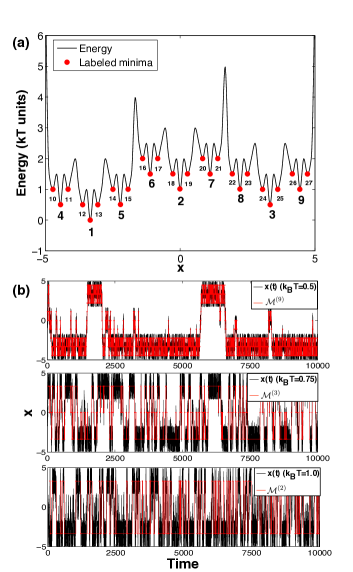
It is useful to illustrate the results of this section on a simple example. Specifically, we consider the motion of a particle by overdamped Langevin dynamics on the one-dimensional potential energy depicted in Fig. 3(a). The governing equation is

$$\gamma\dot{x}(t)=-U^{\prime}(x)+\sqrt{2\beta^{-1}\gamma}\,\eta(t)$$ (37)

where $U^{\prime}(x)$ denotes the derivative of potential energy $U(x)$, $\gamma$ is the friction coefficient (which we will set to $\gamma=1$) and $\eta(t)$ a white-noise such that $\langle\eta(t)\rangle=0$ and $\langle\eta(t)\eta(t^{\prime})\rangle=\delta(t-t^{\prime})$. Typical trajectories solution of (37) at three different temperatures are shown in Fig. 3(b).

As can been seen in Fig. 3(a), the potential has a hierarchical structure with a total of 27 local minima separated by barriers of various heights. Correspondingly, the generator of the process governed by (37), namely the operator

$$\mathcal{L}=-U^{\prime}(x)\partial_{x}+\beta^{-1}\,\partial^{2}_{x}$$ (38)

has a spectrum with several groups of low-lying eigenvalues. This spectrum was obtained by spatial-discretization of (38) on a grid of 200 points, and the ratio of successive eigenvalues are shown in Fig. 4(a) at several different temperatures. Small ratios identify low-lying groups of eigenvalues, and several of them can be seen: $\lambda_{1}/\lambda_{2}$, $\lambda_{2}/\lambda_{3}$, $\lambda_{8}/\lambda_{9}$, and finally $\lambda_{26}/\lambda_{27}$ are all small at temperatures ranging from $\beta^{-1}=0.5$ to $\beta^{-1}=1.0$. The eigenvalues involved in these groups describe processes arising on slow time scales that can be organized as follows: $\lambda_{1}$ is associated with longest timescale of hopping over the largest barrier separating the left basin left centered around milestone 1 and right one centered around milestone 2 in Fig. 3(a); $\lambda_{2}$ is associated with the next longest time hopping over the barrier separating the basin at the extreme left centered around milestone 1 and the one in the center centered around milestone 3; $\lambda_{3}$, …, $\lambda_{8}$ are associated with hoping over the barriers separating milestones $1$, $4$, $5$, milestones $3$, $6$, $7$ and milestones $2$, $8$, $9$; and finally $\lambda_{9}$, …, $\lambda_{27}$ are associated with hoping over the barriers separating milestones $4$, $10$, $11$, milestones $1$, $12$, $13$, etc. From the results in Secs. III.1 and III.2, the existence of the low lying groups also suggests that the continuous-time dynamics can be approximated by Markov chains (i.e MSMs) containing, respectively, 2, 3, 9 and 27 states.

Figure 4: (a) First 30 ratios of consecutive eigenvalues of the generator (38) in a range of temperatures from 0.5 to 1.0. The small ratios are $\lambda_{1}/\lambda_{2}$, $\lambda_{2}/\lambda_{3}$, $\lambda_{8}/\lambda_{9}$ and $\lambda_{26}/\lambda_{27}$. (b) The values of the metastability index $\rho_{\mathcal{M}}$ minimized over index sets $\mathcal{M}$ of increasing cardinal $M$: $\rho_{\mathcal{M}}$ clearly correlates well with the eigenvalue ratios shown in panel (a), and the associated index sets $\mathcal{M}$ permit to identify the target milestones shown in Fig. 3 that capture the slow processes in the system.

Figure 5: The eigenvalues of the MSMs made of the states in $\mathcal{M}^{(2)}$ (circles), $\mathcal{M}^{(3)}$ (diamonds), $\mathcal{M}^{(9)}$ (squares), and $\mathcal{M}^{(27)}$ (stars) are plotted against the eigenvalues of the generator of the original process with the same indices. As can be seen, the MSMs capture the low-lying part of the spectrum accurately, with deviations observed only for the largest eigenvalues in the low-lying group, where metastability becomes weaker.

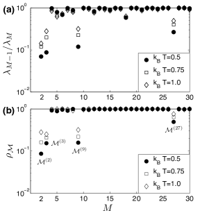
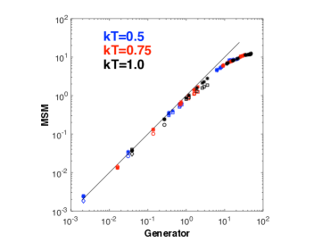
To confirm this prediction, we used the algorithm presented in Sec. II to construct these MSMs. Specifically, we used the 200 discretization points uniformly spaced between $x=-5$ and $x=5$ as trial milestones and computed the matrix entries $\Gamma_{\!i,j}$ defined in (3) from a trajectory obtained by integrating (37). We then minimized the metastability index $\rho_{\mathcal{M}}$ over index sets $\mathcal{M}$ containing from $M=2$ up to $M=30$ indices. The minimum values of $\rho_{\mathcal{M}}$ for each value of $M$ are shown in Fig. 4(b) and, consistent with Bovier’s result, they correlate well with the values of the eigenvalue ratios $\lambda_{M-1}/\lambda_{M}$ shown in Fig. 4(a), thereby confirming that we can use the metastability index $\rho_{\mathcal{M}}$ to identify low-lying groups of eigenvalues. In particular, $\rho_{\mathcal{M}}$ could be made small when $M=2$, 3, 9 and 27, and the corresponding index sets were $\mathcal{M}^{(2)}=\{1,2\}$, $\mathcal{M}^{(3)}=\{1,2,3\}$, $\mathcal{M}^{(9)}=\{1,...,9\}$, and $\mathcal{M}^{(27)}=\{1,...,27\}$. The associated target milestones are shown in Fig. 3(a). They clearly identify the lowest point of the wells on the hierarchical potential landscape $U(x)$. The trajectory projected onto these target milestones when $\mathcal{M}^{(2)}=\{1,2\}$, $\mathcal{M}^{(3)}=\{1,2,3\}$, and $\mathcal{M}^{(9)}=\{1,...,9\}$ are shown in red in Fig. 3(b): these red pieces can be used to calculate the rate matrices $k_{\alpha,\beta}$ of the different MSMs on $\mathcal{M}^{(2)}$, $\mathcal{M}^{(3)}$, $\mathcal{M}^{(9)}$, and $\mathcal{M}^{(27)}$ via maximum likelihood maximization, as explained in Sec. II.4. We can then calculate the spectrum of these rate matrices and compared them to the spectrum of the generator (38) of the original process. The result of these calculation is shown in Fig. 5 which shows that the eigenvalues of these different MSMs do indeed match the low-lying ones of the generator of the original process.

Note that the calculations above to identify target milestones were conducted at different temperatures, and showed that the target milestones were robust for temperature ranging from $\beta^{-1}=0.5$ to $\beta^{-1}=1.0$, even though their corresponding metastability index $\rho_{\mathcal{M}}$ slowly grew with temperature. This is consistent with the fact that the ratios $\lambda_{M-1}/\lambda_{M}$ also grow with temperature, as the system becomes slowly less metastable as it is heated up, with the groups associated with the lowest barriers disappearing first.

Note also that in these calculations, few transitions events between the target milestones were observed (much less in particular that what is required to calculate the rate matrix entries $k_{\alpha,\beta}$ accurately), and yet the procedure was able to identify these milestones correctly.

Figure 6: (a) Trial milestones used to analyze the trajectory from the MD simulation of the GAG peptide at $T=330$ K. These trial milestones are disks centered around grid points in the $(\phi,\psi)$-space, and they are colored according to their free energy $\mathit{\Delta}A_{i}$, whose estimator is given in (16). The states composing the target milesones $\alpha_{R}$, $\alpha_{L}$, $P_{\text{II}}$ and $\alpha_{D}$ are represented as white filled circles. (b) A portion of a $1.3$ $\mu$s MD simulation at $T=330$ K projected onto $\phi$ and $\psi$ (black curve). In red we show the index function $\alpha_{*}(t)$ of the states in the target set $\mathcal{M}^{(4)}=\{\alpha_{R},\alpha_{L},P_{\text{II}},\alpha_{D}\}$.

Figure 7: GAG peptide: Minimum values of the metastability index $\rho_{\mathcal{M}}$ as a function of $M$, along with the index sets $\mathcal{M}$ associated with $\rho_{\mathcal{M}}$ smaller than 1. A Monte Carlo scheme was utilized to perform the minimization.

Figure 8: GAG peptide: Analysis based on the MSM with states in $\mathcal{M}^{(4)}$. (a) Committor probabilities $q_{\alpha_{R}}(i)$. (b) The transition state index $\sigma(i)$, the red regions represents the milestones likely to be part of a TSE; unfilled circles are trial milestones that were visited only once (and hence for which $q_{\alpha}(i)=1$ for some $\alpha$). (c) Hard partitioning of the trial milestones using $\alpha(i)=\operatorname{argmax}_{\alpha\in\mathcal{M}}q_{\alpha}(i)$. (d) Network of the MSM : The numbers of transitions observed between pairs are shown on the edges, and the equilibrium probability of the target milestones are shown next to the nodes.

IV Gly-Ala-Gly peptide

In this section, we use the method outlined in Sec. II to analyze a MD trajectory of a solvated Glycine-Alanine-Glycine peptide (GAG). The GAG peptide was modeled using the CHARMM 27 force field and simulated in a box of 475 TIP3P water molecules using the program NAMD version 2.8 Phillips et al. (2005). After minimization the system was equilibrated for 10ns with the peptide held constrained. The equilibration was followed by a 1.3 $\mu$s production run with Langevin dynamics at 330 K, using a friction constant of 5 ps. The bonds between hydrogens and heavy atoms were kept rigid to allow integration at 2 fs. Frames were saved every 0.5 ps and a total of $2.6\cdot 10^{6}$ trajectory snapshots were collected.

To construct the set of trial milestones, we projected the MD trajectory onto the pair of dihedral angles $(\phi,\psi)$ that corresponds to the central residue alanine. We discretized the $(\phi,\psi)$-space into a square grid of size $8$ deg and used circles of radius $4$ deg around these discretization points as trial milestones – we also used a finer grained definition of the trial milestones, a grid of points at 5 deg but this did not significantly change the results. Only those milestones that we were hit by the trajectory were kept: these consist of the $N=1303$ milestones shown as circles in Fig. 6(a), and colored according to their free energy $\mathit{\Delta}A_{i}$ whose estimator is given in (16). This free energy defines a landscape that is divided in four macro-regions, often labeled as C5, $P_{\text{II}}$, $\alpha_{R}$, $\alpha_{L}$ and $\alpha_{D}$. Interestingly, the overall topography of this landscape is consistent with that obtained in a reference study on a solvated alanine dipeptide Smith (1999) where the $\alpha_{R}$ conformation is the most populated (see the Ramachandran map in Ref. [Iwaoka et al., 2002] for the conformation names and Refs. [Iwaoka et al., 2002; Ding et al., 2003; Weise and Weisshaar, 2003] for comparison with NMR studies on the alanine conformational preferences). Since the target milestones that emerged from our analysis were located in the regions around C5, $P_{\text{II}}$, $\alpha_{R}$, $\alpha_{L}$ and $\alpha_{D}$ (these target milestones are shown as filled white circles in Fig. 6(a)), we used this nomenclature to designate them. Fig. 6(b) shows a portion of the trajectory projected on the angles $\phi$ and $\psi$.

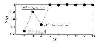
From the MD trajectory the matrix of probabilities $\Gamma_{\!i,j}$ was estimated from (3), and the metastability index $\rho_{\mathcal{M}}$ was minimized over index sets $\mathcal{M}$ of different cardinals $M$. The results are shown in Fig. 7. Two sets of target milestones were found to be clearly metastable: $\mathcal{M}^{(2)}=\{\alpha_{R},\alpha_{L}\}$ with metastability index $\rho_{\mathcal{M}}=0.29$, and $\mathcal{M}^{(4)}=\{\alpha_{R},\alpha_{L},P_{\text{II}},\alpha_{D}\}$ with metastability index $\rho_{\mathcal{M}}=0.45$. A third set of target milestones, $\mathcal{M}^{(3)}=\{\alpha_{R},\alpha_{L},P_{\text{II}}\}$ was also metastable, but with a higher metastability index $\rho_{\mathcal{M}}=0.8$. Interestingly, the index set minimizing $\rho_{\mathcal{M}}$ when $M=5$ was $\mathcal{M}^{(5)}=\{\alpha_{R},\alpha_{L},P_{\text{II}},\alpha_{D},C5\}$, but its metastability index $\rho_{\mathcal{M}}$ was close to 1, i.e. it was not deemed suitable by our analysis to be used to construct an MSM.

Figure 9: Beta3s mini-protein: (a) Trajectory of the dihedral angles $(\phi,\psi)$ of a single amino acid crossing the three circular milestones $0$, $1$, and $2$. The part of the trajectory in red contributes to the statistics of the events $0\to 1$ while the white double stroked portion contributes to the event $1\to 2$. (b) Combinations of the dihedral milestones of two residues into chain milestones (strings). (c) Ranked frequencies of the dihedral milestones prior (black) and after (red) the filtering that yielded a trial set of $N=2120$ milestones with a filter cutoff of 30. The unfiltered ranked frequencies follow the Zipf’s law $1/r^{a}$ with exponent $a\approx 0.76$.

To confirm that the target milestones in $\mathcal{M}^{(2)}$, $\mathcal{M}^{(3)}$ and $\mathcal{M}^{(4)}$ were good core sets to build an MSM (whereas others, including $\mathcal{M}^{(5)}$, were not), we estimated the transition rate matrix entries $k_{\alpha,\beta}$ of the corresponding MSMs using the procedure described in Sec. II.4. We then estimated the empirical first passage time (FPT) distributions from the MD trajectory for the transitions between the states in these MSMs. These were found to be approximately exponential, with decay rates consistent with those deduced from the matrix with entries $k_{\alpha,\beta}$ (data shown in Fig. S1 of the supplementary materials Sup ). This indicates that the dynamics projected on these states is approximately Markovian, and confirms that a low metastability index is indeed a sign of Markovianity. Conversely, the FPT distributions between milestones $C5$ and $P_{\text{II}}$ were non-exponential, which is indicative of the non-Markovian character of these transitions (see Fig. S1(a) in supplementary materials Sup ). Interestingly, this result is consistent with the experimental findings about the non-cooperativity of the alanine $P_{\text{II}}$ conformation in GGAGG peptides due to highly local hydration effects Chen et al. (2004). It is also noteworthy that the transitions between the target milestones occur on different time scales: $\tau(P_{\text{II}}\to\alpha_{R})=0.48$ ns, $\tau(\alpha_{R}\to P_{\text{II}})=0.73$ ns, $\tau(P_{\text{II}}\to\alpha_{L})=9.5$ ns, $\tau(\alpha_{R}\to\alpha_{L})=9.1$ ns, $\tau(\alpha_{L}\to\alpha_{D})=8.5$ ns, $\tau(\alpha_{D}\to\alpha_{L})=2.7$ ns. This explains why different sets of target milestones can be identified, similar to what we observed in the illustrative example of Sec. III.3. Note that the transition time scales between $P_{\text{II}}$ and $\alpha_{R}$ are consistent with the $\approx 1$ ns^-1 interconversion rates reported in earlier studies on a solvated alanine dipeptide Smith (1999); Bolhuis et al. (2000); de Oliveira et al. (2007). Note also that the target milestone $\alpha_{L}$ plays the role of a hub for the transitions involving the left quadrant of the Ramachandran plot with the basin centered in $\alpha_{D}$. That is due to the fact that direct transitions from the helical region $\alpha_{R}$ to the bottom right quadrant are very rare events in a solvated alanine.

Finally, the MSM with the target milestones in $\mathcal{M}^{(4)}$ was used to cluster the state space of the system. These results are shown in Fig. 8. The committor probabilities $q_{\alpha_{R}}(i)$ shown in Fig. 8(a) permit one to assign each of the trial milestones to the target milestones it is most likely to reach next, thereby partitioning the dihedral space into basins (see Fig. 8(c)). In Fig. 8(b) the trial milestones are colored according to the TSE index $\sigma(i)$ defined in (18). The red regions represent the trial milestones $S_{i}$ which are likely to part of a transition state ensemble. Also shown in Fig. 8(d) is the network of the MSM.

V Beta3s mini protein

As a last example we applied our method to analyze a 20 $\mu$s long MD trajectory of the Beta3s peptide in implicit solvent at 330K, where multiple folding/unfolding events were observed. The Beta3s is a 20 residue peptide which is known to assume a triple stranded $\beta$-sheet fold De Alba et al. (1999); Ferrara and Caflisch (2000); Rao and Caflisch (2004); Krivov et al. (2008). The simulation details of the MD data we analyzed here can be found in Ref. Muff and Caflisch (2008). The 20 $\mathrm{\mu s}$ long trajectory is composed of $10^{6}$ microstates saved at a lag-time $\tau=20$ ps. In the context of the GAG peptide (Sec. IV), the torsional angles of the central alanine residue were shown to be sufficiently good descriptors of the conformational space and were used to define the trial milestones. This procedure, however, is not applicable to a 20 residues mini protein such as Beta3s, whose configurational space is much more complex than that of a tri-peptide. For the initial definition of the trial set of milestones several alternatives are in principle viable. Here we used the main dihedral angles along the chain as starting point.

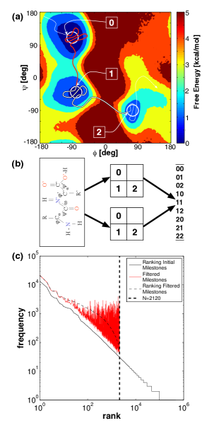
Specifically, the trial milestones were defined at the level of the individual amino acids. For a protein of $R$ residues there are $R-2$ pairs of main dihedral angles $(\phi_{r},\psi_{r})$ along the chain, where $r=2,...,(R-2)$ denotes the residue index. For each of the $R-2$ Ramachandran plots that are associated to a residue, three trial milestones were defined as circles of radius 30 deg, and denoted as milestone $0$, $1$, and $2$. The centers of these circles are located at the minima of the free energy landscape obtained from the empirical $(\phi_{r},\psi_{r})$ probability density of all the residues combined (see the free energy contour plot in Fig. 9(a)) that is estimated from the MD trajectory. The locations of the milestone centers are $(-90,110)$ for state $0$ (beta-sheet region), $(-80,-40)$ for the state $1$ (helix region), and $(75,-90)$ for state $2$ (turn/loop region). In this way, the value of each pair of residue $(\phi_{r},\psi_{r})$ along the MD trajectory is first mapped on a three-letter alphabet, and these letters are then combined into a word, resulting in the representation

$$S_{i}=s^{(2)}s^{(3)}\cdots s^{(R-2)}$$ (39)

where $s^{(r)}\in(0,1,2)$ and $r$ the residue index. For example, the folded state is represented as “$000021000000210000$”. Fig. 9(b) gives a pictorial representation of the construction of symbolic milestones. Since Beta3s is a 20 residues mini-protein, the upper limit of accessible trial milestones constructed this way is therefore $3^{18}\approx 4\cdot 10^{8}$.

Figure 10: Metastability index for the Beta3s peptide at 330K calculated using four different sets of trial milestones obtained with different filtering cutoff. In each case, the procedure identify the same target milestones with metastability index lower than 1..

Figure 11: Network of the MSM for Beta3s based on $\mathcal{M}^{(8)}$. The nodes on the left side of the network have a high entropy while those on the right side have low energy. The node involving the triple stranded folded state lies at the center of a large basin in which energy and entropy compensate each other. The thickness of the edges between pairs of target milestones on the network is proportional to the total number of transitions observed between these milestones: these numbers are also reported in figure. Each node of the network is represented along with the ensemble of structures associated to the most populated trial milestone it contains.

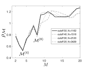
In practice, not all these trial milestones were visited even once along the trajectory, and some were visited much more often than others. To avoid using trial milestones visited too few times, we filtered out the milestones that were visited less than a threshold value of times. The first step of dihedral milestoning gave a total number of $N_{0}=469677$ dihedral strings, 373456 of which were visited only once, which is about $\sim$37% of the whole set. Interestingly, the ranked distribution of the visting frequencies follows a Zipf’s law decay, namely a power law $\sim 1/r^{a}$ with $r$ the rank and $a=0.76$ the exponent (see Figure 9(c)). Different frequency thresholds were used to filter out trial milestones. Cutoffs corresponding to 20, 30, 40, and 50 reduced the number of trial milestones to 3439, 2120, 1516, and 1162, respectively. All these four sets of trial milestones were used to process the MD trajectory and estimate the probabilities $\Gamma_{\!i,j}$. The metastability index $\rho_{\mathcal{M}}$ was calculated for target sets $\mathcal{M}$ with cardinality in the range $M=2,...,20$. Fig. 10 shows the result of this calculation. Irrespective of the cutoffs used to define the set of trial milestones, the resulting target sets were robust in the range $M=2,...,8$ where at the low values of $\rho_{\mathcal{M}}\lesssim 1$.

To better understand the conformational dynamics of the Beta3s peptide, we used the tools introduced in Sec. II.5. The committor probability $q_{\alpha}(i)$ (obtained from (17)) permits one to perform a soft partitioning of the trial milestones. Each target set milestone $B_{\alpha}$ is the center of a partition with statistical weight $\pi_{\alpha}$ that is obtained from (12), and from which the free energy $\mathit{\Delta}G_{\alpha}$ is determined from (13). This free energy can then be decomposed into energetic and entropic contributions according to (19) and (21). Here the effective energy of the system is identified as the sum of two contributions: $\bar{E}=E_{\rm charmm}+E_{\rm sasa}$ where $E_{\rm charmm}$ is the total potential energy in the CHARMM force field and $E_{\rm sasa}$ is the solvent accessible term due to the implicit solvation model. Using (20) we obtained $\bar{E}=-37.9\pm 11.1$ kcal/mol as mean effective energy of the entire set of conformation sampled.

Markov State Model
id	Symbolic Milestone	$\pi_{\alpha}$	$N_{\alpha}$	$\mathit{\Delta}G_{\alpha}$	$\mathit{\Delta}E_{\alpha}$	$-T\mathit{\Delta}S_{\alpha}$
		[%]		[kcal/mol]	[kcal/mol]	[kcal/mol]
1	000021000000210000	76	48	0.2	-0.6	0.8
106	111111111111100000	8.2	42	1.6	4.9	-3.3
164	001211001000210010	3.1	9	2.3	-5.5	7.8
241	111111111111111111	3.1	37	2.3	4.7	-2.5
264	010001111111111111	4.5	33	2.0	5.1	-3.0
319	001111000011111000	2.3	19	2.5	-3.6	6.0
473	001111000000200000	1.4	23	2.8	-2.2	4.9
843	001111000111210010	1.4	5	2.8	-2.8	5.7

Table 1: Beta3s mini-protein: Target milestones members of the set $\mathcal{M}^{(8)}$, along with their thermodynamical parameters.

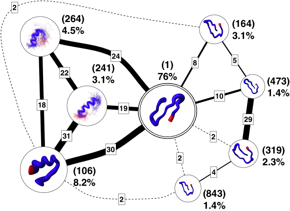
We focused our analysis on the target set $\mathcal{M}^{(8)}$ that resulted the largest metastable target set with $\rho_{\mathcal{M}}<1$. The committor probability $q_{\alpha}(i)$ is calculated from the time series of trial milestones, with $\alpha\in\mathcal{M}^{(8)}$. Table 1 lists the statistical weights of the most populated states in the MSM build on $\mathcal{M}^{(8)}$. The mean effective energies $\mathit{\Delta}E_{\alpha}$ are also reported in Table 1, along with the entropy contributions $-T\mathit{\Delta}S_{\alpha}$ to the free energy $\mathit{\Delta}G_{\alpha}$. The basin centered around the target milestone associated with the folded state (id 1 in table 1) has a statistical weight $\pi_{1}$ of about 76%, meaning that Beta3s spends about the 3/4 of the simulation time in this basin. As expected for a folded state, it has an energetic advantage ($\mathit{\Delta}E_{1}=-0.6$ kcal/mol) which compensates its entropic disadvantage ($-T\mathit{\Delta}S_{1}$=0.8 kcal/mol). The other basins identified in the target set $\mathcal{M}^{(8)}$ include helical and beta-curl type configurations. Interestingly, the helical basins (id 106, 241, and 264 in Table 1) are entropically favored ($\Delta S_{\alpha}<0$ and $\Delta E_{\alpha}>0$) while the beta-curl states are energetically favored basins (id 164, 319, 473, and 843 in Table 1) with $\Delta S_{\alpha}<0$ and $\Delta E_{\alpha}<0$. The statistical error on the mean effective energies $\Delta E_{\alpha}$ is estimated as $std(\Delta E_{\alpha})/\sqrt{N_{\alpha}}$ where $std(\Delta E_{\alpha})$ is a standard deviation and $N_{\alpha}$ is the number of times the system enters a target milestone $B_{\alpha}$. The values of $N_{\alpha}$ are reported in Table 1. The statistical errors on $\Delta E_{\alpha}$ are reported in Fig. S4 of the supplementary materials Sup along with the empirical probability density functions of the effective energy for each of the target milestones $B_{\alpha}$. While these errors are large, the information contained in $\mathit{\Delta}E_{\alpha}$ remains statistically significant.

Fig. 11 shows the network of the MSM built on the target set $\mathcal{M}^{(8)}$. Notably, the folded state lies in between the helical region, which is entropically favored, and the beta-curl region, which is energetically favored. Except very rare direct connections between the helical and beta-curl regions, most of the transitions between the helix and beta-curl basins occur via the folded state. Thus, as was remarked elsewhere Bowman and Pande (2010), the folded state is not only the region of the configurational space where energy and entropy compensate each other, but it also plays the role of a dynamical hub in the network. This observation is confirmed by the high number of times the target milestone associated to the folded state is revisited ($N_{1}=48$ is the highest values observed, see $N_{\alpha}$ column in Table 1).

The high entropy character of the helical states is also reflected by the high connectivity within the helical region (left side of the network shown in Fig. 11) and the comparable values of $N_{\alpha}$ with that of the folded state ($N_{106}=42$, $N_{241}=37$, and $N_{264}=33$ in Table 1). On the contrary, the beta-curl states (right side of the network shown in Fig. 11) are less connected ($N_{164}=9$, $N_{319}=19$, $N_{473}=23$, and $N_{843}=5$). This is consistent with the observation reported in Muff and Caflisch (2008) that these beta-curl states act as kinetic traps.

The probability distributions of FPT from the folded state to the other member of the target set and back are fairly well described by an exponential decay (see Fig. S2 and S3 in the supplementary materials Sup ). This indicates that the reduced dynamics of the Beta3s to a MSM built on the target set $\mathcal{M}^{(8)}$ is approximatively Markovian. Interestingly, the emerging picture from the network representation in Fig. 11 is qualitatively consistent with the simplified kinetic network representation proposed in Ref. Krivov et al. (2008).

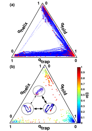
The committor probability $q_{\alpha}(i)$ calculated for the target set $\mathcal{M}^{(8)}$ allows one to project the configurational space onto a simplex. Three aggregated committor probabilities are defined as $q_{{\rm fold}}=q_{1}$ for the folded state, $q_{{\rm helix}}=q_{106}+q_{241}+q_{264}$ for the helix state, and $q_{{\rm trap}}=q_{164}+q_{319}+q_{473}+q_{843}$ for the beta-curl state (see Table 1 for the state indexes). By definition of committor probability one has $q_{\rm fold}+q_{\rm helix}+q_{\rm trap}=1$. Fig. 12 shows the simplex representation of the aggregated committor probabilities in a triangular plot. Fig. 12(a) shows the time series of the committor probabilities $q_{\rm fold}(i_{*}(t)),q_{\rm helix}(i_{*}(t)),q_{\rm trap}(i_{*}(t))$ projected onto a triangular plot. Interestingly, the conformers are clustered around the three vertexes of the triangular plot. The blue lines represent direct transitions between conformer and only 4 direct transitions link the helix channel to the trap channel. Fig. 12(b) shows a triangular scatter plot of the committor probabilities with the points colored according to their TSE index $\sigma(i)$ defined in (18). Red points correspond to milestones belonging to transition state ensembles. For instance, the channel connecting the helix to the fold basin is composed by milestones $S_{i}$ such that $q_{\rm fold}\approx q_{\rm helix}\approx 0.5$. Similarly, along the channel Trap$\leftrightarrow$Fold one has milestones $S_{i}$ with $q_{\rm fold}\approx q_{\rm trap}\approx 0.5$. The simplex representation in Fig. 12 corroborates the observation that the folded state acts as a kinetic hub Muff and Caflisch (2008), and it also suggests that Beta3s oscillates between two extreme conformational regions: a low energy one versus a high entropy one.

Figure 12: Beta3s peptide: (a) Simplex representation of the aggregated committors such that $q_{{\rm fold}}=q_{1}$, $q_{{\rm helix}}=q_{106}+q_{241}+q_{264}$ and $q_{{\rm trap}}=q_{164}+q_{319}+q_{473}+q_{843}$ (these indices are the same as those used in Fig. 11). The continuous blue line represent the time series $q_{{\rm fold}}(i_{*}(t))$, $q_{{\rm helix}}(i_{*}(t))$ and $q_{{\rm trap}}(i_{*}(t))$ Only 4 transition events connect directly the helix and beta regions. (b) Same representation with nodes colored according 1 to the TS index $\sigma(i)$ defined in (18).

VI Conclusions

Despite their growing popularity to analyze and interpret molecular dynamics (MD) simulations, Markov State Models (MSMs) remain somewhat tricky to use and justify. How to pick the states over which to build the MSM and how to assess its accuracy are nontrivial issues that are related to the degree to which the dynamical coarse-graining over these states preserves the Markovianity of the original system. Typically, states in MSMs are picked in a somewhat ad hoc fashion, and their quality is assessed a posteriori via Markovianity tests. In this paper, we propose a strategy that may help systematize the operation of MSM building. It is based on the observation that, in metastable systems, the states in an MSM should be hubs to which the trajectory has a high probability to return often, and between which it seldom transitions. These intuitive properties can be captured via a metastability index that measures how good a set of target milestones chosen among trial ones is: the smaller its metastability index, the better the target milestones it contains are as hubs. This metastability index is not a new concept: it was introduced in a closely related form in potential theoretic approaches to metastability. Our main goal in this paper was to show that this index can also be turned into a practical computational tool for the identification of good target milestones upon which to build accurate MSMs. As we shown here the procedure is simple to use, it does not require to make Markovian assumptions at the intermediate stages of the construction (in particular, the jumps between the trial milestones could be correlated and non-Markovian), and it has the added advantage that it allows one to cluster the system’s state space a posteriori and identify the transition state ensembles (TSEs) between the target milestones. Here, these features were illustrated on a collections of examples of increasing complexity. In particular, our last test case involving the Beta3s mini-protein, showed that the method can reveal interesting properties of the folding landscape of proteins, including the presence of kinetic traps and misfolded states on the way to the native state, and how these features affects the folding and unfolding pathways of the protein. We certainly hope that the technique will be similarly useful to analyze the dynamics of other proteins and macromolecules.

Appendix A Derivation of (27)

In this section a proof of (27) is given in case of a Markov process with generator $L_{i,j}$ and transition probability $P_{i,j}=L_{i,j}/\sum_{k\not=i}L_{i,k}$, $i\not=j$, $P_{i,i}=0$. To begin, recall that the MFPT $\tau_{i,j}$ from state $i$ to state $j$ is the solution to

$$\sum_{k=1}^{N}L_{i,k}\tau_{k,j}=-1,\quad\text{for}\ \ i\not=j,\quad\text{and}\quad\tau_{j,j}=0$$ (40)

while the MRT is given by

$$\tau_{i}=(\sum_{j\neq i}L_{i,j})^{-1}+\sum_{k=1}^{N}P_{i,k}\tau_{k,i}$$ (41)

where the first term at the right hand-side accounts for the mean time to exit $i$ to some state $j\not=i$, and the second for the mean time to come back from any such state $j\not=i$ to $i$. We are interested to find an expression for the probabilities $\Gamma_{\!i,j}$ as a function of the MFPT and MRT. Since $\Gamma_{\!i,j}=\sum_{k}P_{i,k}q_{i,j}(k)$, we can equivalently express the committor function $q_{i,j}(k)$ in terms of MFPT and the MRT. We claim that

$$q_{i,j}(k)=\frac{\tau_{k,i}-\tau_{k,j}+\tau_{i,j}}{\tau_{i,j}+\tau_{j,i}}$$ (42)

Let us check that this relation holds by verifying that the function $q_{i,j}(k)$ defined this way satisfies $q_{i,j}(i)=0$, $q_{i,j}(j)=1$ and $\sum_{l\in S}L_{k,l}q_{i,j}(l)=0$ for $k\notin\{i,j\}$. The two boundary conditions are trivially verified and the third condition is

$$\sum_{l=1}^{N}L_{k,l}q_{i,j}(l)$$ (43)

$$\quad=\frac{1}{\tau_{i,j}+\tau_{j,i}}\sum_{k,l=1}^{N}L_{k,l}(\tau_{l,i}-\tau_{l,j}+\tau_{i,j})$$

$$\quad=0$$

where we have used (40). We can now calculate $\Gamma_{\!i,j}$ using (42) and (25)

$$\Gamma_{\!i,j} =\sum_{k=1}^{N}P_{i,k}q_{i,j}(k)$$ (44)

$$=\frac{(\sum_{k\neq i}L_{i,k})^{-1}}{\tau_{i,j}+\tau_{j,i}}\sum_{k=1}^{N}L_{i,k}(\tau_{k,i}-\tau_{k,j}+\tau_{i,j})$$

$$=\frac{(\sum_{k\neq i}L_{i,k})^{-1}}{\tau_{i,j}+\tau_{j,i}}\left(\sum_{k=1}^{N}L_{i,k}\tau_{k,i}+1\right)$$

$$=\frac{\tau_{i}}{\tau_{i,j}+\tau_{j,i}}$$

where we used (40) and (41). Thus, for any pair of states $(i,j)$, the probability $\Gamma_{\!i,j}$ can be computed from the MFPTs and MRTs only.

References

- Schutte et al. (1999) C. Schutte, A. Fischer, W. Huisinga, and P. Deuflhard, J. Comput. Phys. 151, 146 (1999).
- Swope et al. (2004) W. C. Swope, J. W. Pitera, and F. Suits, J. Phys. Chem. B 108, 6571 (2004).
- Chodera et al. (2007) J. D. Chodera, N. Singhal, V. S. Pande, K. A. Dill, and W. C. Swope, J. Chem. Phys. 126, 155101 (2007).
- Noe and Fischer (2008) F. Noe and S. Fischer, Current Opinion in Structural Biology 18, 154 (2008).
- Schütte et al. (2011) C. Schütte, F. Noe, J. Lu, M. Sarich, and E. Vanden-Eijnden, J. Chem. Phys. 134, 204105 (2011).
- Schütte and Sarich (2013) C. Schütte and M. Sarich, Metastability and Markov state models in molecular dynamics: modeling, analysis, algorithmic approaches, Vol. 24 (American Mathematical Soc., 2013).
- Bowman et al. (2013) G. R. Bowman, V. S. Pande, and F. Noé, An introduction to markov state models and their application to long timescale molecular simulation, Vol. 797 (Springer Science & Business Media, 2013).
- Shaw et al. (2010) D. Shaw, P. Maragakis, K. Lindorff-Larsen, S. Piana, R. Dror, M. Eastwood, J. Bank, J. Jumper, J. Salmon, Y. Shan, et al., Science 330, 341 (2010).
- Stone et al. (2007) J. E. Stone, J. C. Phillips, P. L. Freddolino, D. J. Hardy, L. G. Trabuco, and K. Schulten, J. Comput. Chem. 28, 2618 (2007).
- Voelz et al. (2010) V. A. Voelz, G. R. Bowman, K. Beauchamp, and V. S. Pande, J. Am. Chem. Soc. 132, 1526 (2010).
- McGibbon et al. (2014) R. T. McGibbon, C. R. Schwantes, and V. S. Pande, J. Phys. Chem. B 118, 6475 (2014).
- Sultan et al. (2014) M. M. Sultan, G. Kiss, D. Shukla, and V. S. Pande, J. Chem. Theory Comput. 10, 5217 (2014).
- Martini et al. (2016) L. Martini, A. Kells, G. Hummer, N.-V. Buchete, and E. Rosta, ArXiv e-prints (2016), arXiv:1605.04328 [physics.chem-ph] .
- Buchete and Hummer (2008) N. Buchete and G. Hummer, J. Phys. Chem. B 112, 6057 (2008).
- Faradjian and Elber (2004) A. K. Faradjian and R. Elber, J. Chem. Phys. 120, 10880 (2004).
- Vanden-Eijnden et al. (2008) E. Vanden-Eijnden, M. Venturoli, G. Ciccotti, and R. Elber, J. Chem. Phys. 129, 174102 (2008).
- Vanden-Eijnden and Venturoli (2009) E. Vanden-Eijnden and M. Venturoli, J. Chem. Phys. 130, 194101 (2009).
- Krivov and Karplus (2006) S. V. Krivov and M. Karplus, J. Phys. Chem. B 110, 12689 (2006).
- Sarich et al. (2010) M. Sarich, F. Noé, and C. Schütte, Multiscale Model. Sim. 8, 1154 (2010).
- Beauchamp et al. (2011) K. A. Beauchamp, G. R. Bowman, T. J. Lane, L. Maibaum, I. S. Haque, and V. S. Pande, J. Chem. Theory Comput. 7, 3412 (2011).
- Vitalis and Caflisch (2012) A. Vitalis and A. Caflisch, J. Chem. Theory Comput. 8, 1108 (2012).
- Fac̆kovec et al. (2015) B. Fac̆kovec, E. Vanden-Eijnden, and D. J. Wales, J. Chem. Phys. 143, 044119 (2015).
- Bovier et al. (2002) A. Bovier, M. Eckhoff, V. Gayrard, and M. Klein, Communications in mathematical physics 228, 219 (2002).
- Bovier et al. (2004) A. Bovier, M. Eckhoff, V. Gayrard, and M. Klein, J. Eur. Math. Soc. 6, 399 (2004).
- Bovier et al. (2005) A. Bovier, V. Gayrard, and M. Klein, J. Eur. Math. Soc. 7, 69 (2005).
- E and Vanden-Eijnden (2006) W. E and E. Vanden-Eijnden, J. Stat. Phys. 123, 503 (2006).
- Metzner et al. (2009) P. Metzner, C. Schuette, and E. Vanden-Eijnden, Multiscale Model. Sim. 7, 1192 (2009).
- E and Vanden-Eijnden (2010) W. E and E. Vanden-Eijnden, Annu. Rev. Phys. Chem. 61, 391 (2010).
- Phillips et al. (2005) J. Phillips, R. Braun, W. Wang, J. Gumbart, E. Tajkhorshid, E. Villa, C. Chipot, R. Skeel, L. Kale, and K. Schulten, J. Comput. Chem. 26, 1781 (2005).
- Smith (1999) P. E. Smith, J. Chem. Phys. 111, 5568 (1999).
- Iwaoka et al. (2002) M. Iwaoka, M. Okada, and S. Tomoda, J. Mol. Struct. 586, 111 (2002).
- Ding et al. (2003) L. Ding, K. Chen, P. Santini, Z. Shi, and N. Kallenbach, J. Am. Chem. Soc. 125, 8092 (2003).
- Weise and Weisshaar (2003) C. Weise and J. Weisshaar, J. Phys. Chem. B 107, 3265 (2003).
- (34) “See supplemental material at [url will be inserted by aip] that include the first passage times distributions for the gag peptide and beta3s mini-protein, and the statistical errors on the effective energies of the beta3s mini protein.” .
- Chen et al. (2004) K. Chen, Z. Liu, and N. Kallenbach, Proc Natl Acad Sci U S A 101, 15352 (2004).
- Bolhuis et al. (2000) P. G. Bolhuis, C. Dellago, and D. Chandler, Proc. Natl. Acad. Sci. USA 97, 5877 (2000).
- de Oliveira et al. (2007) C. A. F. de Oliveira, D. Hamelberg, and J. A. McCammon, J. Chem. Phys. 127, 175105 (2007).
- De Alba et al. (1999) E. De Alba, J. Santoro, M. Rico, and M. A. Jiménez, Prot. Sci. 8, 854 (1999).
- Ferrara and Caflisch (2000) P. Ferrara and A. Caflisch, Proc. Natl. Acad. Sci. USA 97, 10780 (2000).
- Rao and Caflisch (2004) F. Rao and A. Caflisch, J. Mol. Biol. 342, 299 (2004).
- Krivov et al. (2008) S. V. Krivov, S. Muff, A. Caflisch, and M. Karplus, J. Phys. Chem. B 112, 8701 (2008).
- Muff and Caflisch (2008) S. Muff and A. Caflisch, Proteins 70, 1185 (2008).
- Bowman and Pande (2010) G. R. Bowman and V. S. Pande, Proc. Natl. Acad. Sci. USA 107, 10890 (2010).