Cosmology with photometric weak lensing surveys: constraints with redshift tomography of convergence peaks and moments

Abstract

Weak gravitational lensing is becoming a mature technique for constraining cosmological parameters, and future surveys will be able to constrain the dark energy equation of state $w$. When analyzing galaxy surveys, redshift information has proven to be a valuable addition to angular shear correlations. We forecast parameter constraints on the triplet $(\Omega_{m},w,\sigma_{8})$ for an LSST-like photometric galaxy survey, using tomography of the shear-shear power spectrum, convergence peak counts and higher convergence moments. We find that redshift tomography with the power spectrum reduces the area of the $1\sigma$ confidence interval in $(\Omega_{m},w)$ space by a factor of 8 with respect to the case of the single highest redshift bin. We also find that adding non-Gaussian information from the peak counts and higher-order moments of the convergence field and its spatial derivatives further reduces the constrained area in $(\Omega_{m},w)$ by a factor of 3 and 4, respectively. When we add cosmic microwave background parameter priors from Planck to our analysis, tomography improves power spectrum constraints by a factor of 3. Adding moments yields an improvement by an additional factor of 2, and adding both moments and peaks improves by almost a factor of 3, over power spectrum tomography alone. We evaluate the effect of uncorrected systematic photometric redshift errors on the parameter constraints. We find that different statistics lead to different bias directions in parameter space, suggesting the possibility of eliminating this bias via self-calibration.

I Introduction

Weak gravitational lensing is a promising technique to probe the large scale structure of the universe in which the tracers are intrinsically unbiased (Schneider, 2005). This technique has the potential of significantly improving the constraints on the dark energy equation of state parameter $w$ because it is most sensitive to the matter density fluctuations at the non–linear stage. Cosmology inferences from weak lensing observations have been produced for past (CFHTLenS (Heymans et al., 2012), COSMOS (Koekemoer et al., 2007)) and current (DES (Gruen et al., 2016)) surveys, and are being planned for future experiments as well (e.g. LSST (LSST Dark Energy Science Collaboration, 2012), WFIRST (Spergel et al., 2015), Euclid (Amiaux et al., 2012)). Because of the non-linear nature of the density fluctuations probed by weak lensing, cosmological information might leak from quadratic statistics (such as two-point functions and power spectra) into more complicated non-Gaussian statistics, for which forward modeling requires numerical simulations of cosmic shear fields.

Several different examples of these non-Gaussian statistics, and their cosmological information content, have been studied in the past as well (see (Kratochvil et al., 2012; Yang et al., 2011; Marian et al., 2009; Takada and Jain, 2002, 2003, 2004; Bergé et al., 2010; Dietrich and Hartlap, 2010) for a non-comprehensive list). The constraining power of weak lensing power spectra with the addition of redshift tomography information have been extensively investigated in the literature (see e.g. (Song and Knox, 2004; Fang and Haiman, 2007; Huterer, D. and Takada, M. and Bernstein, G. and Jain, B., 2006)). In this work we concentrate on the constraining power of a subset of non-Gaussian statistics, combined with redshift tomography in an LSST-like survey. (Martinet et al., 2015) investigated the cosmological constraining power of shear peaks tomography. Previous work on redshift tomography with weak lensing Minkowski functionals is also present in the literature (Kratochvil et al., 2012).

Tomography relies on assigning accurate redshifts to galaxies. We therefore also investigate the effects of uncorrected photometric redshift systematics on parameter constraints when using redshift tomography. This work is organized as follows: in § II we outline the shear simulations we use in this work, followed by descriptions of the convergence reconstruction procedure, forward modeling of galaxy shape and photometric redshift systematics, and the parameter-inference techniques we used to forecast constraints on cosmology. In § III we present our main results, which we discuss in § IV. In § V we present our conclusions as well as prospects for future work.

II Methods

II.1 Cosmic shear simulations

We review the procedure used for generating simulated shear catalogs. We consider a fiducial flat $\Lambda$CDM universe with parameters $(h,\Omega_{m},\Omega_{\Lambda},\Omega_{b},w,\sigma_{8},n_{s})=(0.72,0.26,0.74,0.046,-1,0.8,0.96)$ (Hinshaw et al., 2013; Planck Collaboration et al., 2015). We examine different variations of the $\mathbf{p}=(\Omega_{m},w,\sigma_{8})$ triplet and run one $N$–body simulation for each choice of $\mathbf{p}$, using the public code Gadget2 (Springel, 2005). The simulations have a comoving box size of $L_{b}=260\,{\rm Mpc}/h$ and contain $512^{3}$ dark matter particles, which correspond to a mass resolution of $M_{p}\approx 10^{10}M_{\rm sun}$ per particle.

The largest mode observed in our $N$–body simulations corresponds to a wavenumber of $k_{b}\approx 1/L_{b}\approx 0.004h{\rm Mpc}^{-1}$. For the sake of recovering cosmological information from WL, this limitation does not create a concern, as several authors (see (Fang and Haiman, 2007) for example) have shown that modes above $L_{b}$ contribute very little to parameter constraints. Moreover, the purpose of this work is to estimate the parameter constraints achievable in a weak lensing analysis incorporating tomography, not to produce simulations accurate enough for analyzing the data set that will be available from LSST and other surveys a decade hence. To analyze the datasets that these surveys will produce, mode couplings between large and small scales, which can cause effects such as super sample covariance (Sato et al., 2009; Takada and Hu, 2013; Mohammed et al., 2016), will need to be included. Baryonic effects will need to be included as well. Larger and more accurate $N$–body simulation techniques are currently under development in the community for this purpose (Heitmann et al., 2015; Habib et al., 2016).

The three dimensional outputs of the $N$–body simulations are sliced in sequences of two dimensional lenses $120\,{\rm Mpc}$ thick, which are lined up perpendicular to the line of sight between the observer on Earth and a source at redshift $z_{s}$. We make use of the multi–lens–plane algorithm (Jain et al., 2000; Hilbert et al., 2009) to trace the deflections of light rays originating at $z=0$ through the system of lenses out to redshift $z$. To accomplish this task, we make use of the LensTools (Petri, 2016a, b) implementation of the multi–lens–plane algorithm. An observed galaxy position $\boldsymbol{\theta}$ on the sky today corresponds to a real galaxy angular position $\boldsymbol{\beta}(\boldsymbol{\theta},z_{s})$, which can be calculated using the LensTools pipeline by solving the ordinary differential lens equations up to redshift $z_{s}$. The Jacobian of $\boldsymbol{\beta}(\boldsymbol{\theta},z_{s})$ is a $2\times 2$ matrix that contains information about the cosmic shear field at $\boldsymbol{\theta}$ integrated along the line of sight.

$$\frac{\partial\beta_{i}(\boldsymbol{\theta},z_{s})}{\partial\theta_{j}}=\begin{pmatrix}1-\kappa(\boldsymbol{\theta})-\gamma^{1}(\boldsymbol{\theta})&-\gamma^{2}(\boldsymbol{\theta})\\ -\gamma^{2}(\boldsymbol{\theta})&1-\kappa(\boldsymbol{\theta})+\gamma^{1}(\boldsymbol{\theta})\\ \end{pmatrix}$$ (1)

The quantities that appear in equation (1) are the convergence $\kappa$, which is the source magnification due to lensing, and the cosmic shear $\boldsymbol{\gamma}$, which is a measurement of the source ellipticity due to lensing from large scale structure, assuming the non-lensed shape is a circle.

We simulate $N_{g}=10^{6}$ random galaxy positions $\{\boldsymbol{\theta}_{g}\}$ distributed uniformly in a field of view of size $\theta_{\rm FOV}^{2}=(3.5{\rm deg})^{2}$, which correspond to a galaxy surface density of $n_{g}=22\,\rm{arcmin}^{-2}$. The galaxies have a distribution in redshift which mimics the one expected in the LSST survey,

$$n(z)=n_{0}\left(\frac{z}{z_{0}}\right)^{2}\exp\left(-\frac{z}{z_{0}}\right),$$ (2)

with $z_{0}=0.3$ and $n_{0}$ a normalization constant fixed so that $n(z)$ integrates to the total number of galaxies $N_{g}$. The galaxies have a maximum redshift $z_{\rm max}=3$. For each galaxy, we compute the cosmic shear at $\boldsymbol{\theta}_{g}$ using equation (1), producing a shear catalog $\{\boldsymbol{\gamma}_{g}\}$. Different random realizations of a shear catalog $\{\boldsymbol{\gamma}_{g}\}_{r}$ can be obtained rotating and periodically shifting the large scale structure in the $N$–body snapshots according to the procedure explained in (Petri et al., 2016). We produce $N_{r}=16000$ pseudo–independent realizations of the shear catalog $\{\boldsymbol{\gamma}_{g}\}$. These shear realizations all together cover 10 times the total survey area of LSST. We repeat the above procedure for $P=100$ different combinations of the parameter triplet $\mathbf{p}$, sampled according to a Latin hypercube scheme. The sampling procedure is the same as described in (Petri et al., 2015; Liu et al., 2015). The parameter space sampling we adopted for our simulations is shown in Figure 1.

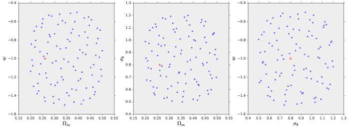
Figure 1: Parameter space sampling chosen for our simulations. We show the sampling in the $(\Omega_{m},w)$ (left), $(\Omega_{m},\sigma_{8})$ (center) and $(\sigma_{8},w)$ (right) projections of the parameter space. The fiducial cosmology has been marked in red.

For each of the parameter choices in Figure 1, the $N$–body initial conditions are generated using the same random seed. In addition to these simulations, we produce simulated shear catalogs for a fiducial $\Lambda$CDM universe with $\mathbf{p}_{0}=(0.26,-1,0.8)$. In this case the randomization procedure is based on 5 independent $N$–body simulations, and the same number $N_{r}=16000$ of pseudo–independent catalog realizations is produced. This additional simulation set serves two purposes: it provides an independent dataset from which to measure covariance matrices, and it provides a way to construct simulated observations that are independent of the simulations on which the cosmological forward model is trained. For the fiducial dataset we chose to base the shear randomization procedure on 5 independent $N$–body simulations to ensure the independence of the $N_{r}$ realizations for the purpose of estimating covariance matrices. Ref. (Petri et al., 2016) recently showed that, even with only one $N$–body simulation a few $10^{4}$ independent realizations can be produced.

II.2 Forward modeling of systematics

We next give an overview of the shear systematics included in this work.

The measured galaxy ellipticity $\boldsymbol{\epsilon}$ is an estimate of the cosmic shear $\boldsymbol{\gamma}$ due to large scale structure if the non–lensed galaxy shape is a circle. Because the galaxies have intrinsic noncircular shapes, the measured galaxy ellipticity $\boldsymbol{\epsilon}_{\rm m}$ is the sum of a cosmic shear term and the intrinsic ellipticity (galaxy shape noise) (Schneider, 2005)

$$\boldsymbol{\epsilon}_{\rm m}=\boldsymbol{\gamma}+\boldsymbol{\epsilon}_{\rm n}$$ (3)

where $\boldsymbol{\epsilon}_{\rm n}$ is a random Gaussian variable with zero mean and redshift dependent variance $\sigma_{n}(z_{s})=0.15+0.035z_{s}$. This is equivalent to saying that the cosmic shear inferred from ellipticity observations $\boldsymbol{\gamma}_{\rm m}$ can be written as the sum of the true cosmic shear plus a noise term $\boldsymbol{\gamma}_{\rm n}$ with the same statistical properties as $\boldsymbol{\epsilon}_{\rm n}$. We add independent random realizations of the shape noise $\boldsymbol{\gamma}_{\rm n}$ to each of the $N_{r}$ shear catalogs. Each shape noise realization is generated with a different random seed. The same random seeds are used to generate shape noise catalogs across simulations with different cosmological parameters $\{\mathbf{p}_{i}\}$.

In addition to shape noise contributions to the observed galaxy ellipticity, we consider photometric redshift errors as an additional contamination in the simulated catalogs. In photometric surveys such as LSST, the source redshift $z_{s}$ is estimated measuring the source luminosity in a small finite set of optical frequency bands. Using this compressed luminosity information rather than the full spectrum introduces biases in redshift estimation. Forward modeling of the cosmic shear using the procedure described in § II.1, as well as the shape noise contributions, assume a correct redshift distributions $n(z)$. An incorrect binning of observed galaxy redshifts according to the measured photometric distribution $n_{p}(z_{p})$ can propagate the redshift measurement errors all the way to cosmological parameter constraints if the latter take advantage of redshift tomography. One of the goals of this work is to evaluate the size of this effect, assuming photometric redshift errors (photo-$z$) are left uncorrected.

The study of photometric redshift errors is an active subject of research, and includes investigation of techniques such as spectroscopic calibration, catastrophic errors and cross-correlation techniques that we do not explore in this work (see for example (Zhan, 2006; LSST Science Collaboration et al., 2009) for a more thorough discussion). We model the effect of photo-$z$ errors as a constant bias term $b_{\rm ph}(z_{s})$ plus a random Gaussian component with variance $\sigma_{\rm ph}(z_{s})$,

$$z_{p}(z_{s})=z_{s}+b_{\rm ph}(z_{s})+\sigma_{\rm ph}(z_{s})\mathcal{N}(0,1),$$ (4)

where $\mathcal{N}(0,1)$ is the standard normal distribution. We bin the $N_{g}$ galaxies in our simulated catalogs into 5 redshift bins $\bar{z}_{b}$, $b=1...5$. Several models have been proposed in the literature for the photometric bias $b_{\rm ph}(z_{s})$ (see for example (Huterer, D. and Takada, M. and Bernstein, G. and Jain, B., 2006)) and variance $\sigma_{\rm ph}(z_{s})$ (see for example (LSST Science Collaboration et al., 2009)). We chose the photo-$z$ bias and variance functions in equation (4) to be the science requirements contained in the LSST Science Book (LSST Science Collaboration et al., 2009), namely $b(z_{s})=0.003(1+z_{s})$ and $\sigma(z_{s})=0.02(1+z_{s})$.

Figure 2: Galaxy distribution assumed throughout this work (see equation (2)), along with the choice of the redshift bins $\bar{z}_{b}$. Our galaxy sample consists of $N_{g}=10^{6}$ galaxies. The figure shows the number of galaxies $N_{g}(z)$ at each redshift $z$.

We generate simulated observations by applying an independent random realization of the photo-$z$ correction (4) to each catalog realization in the fiducial cosmology $\mathbf{p}_{0}$ and by re–binning the galaxies according to their photometric redshifts $z_{p}$. In the remainder of the paper we use the following notation: we indicate a shear realization $r$ in cosmology $\mathbf{p}$ with shape noise added as $\hat{\boldsymbol{\gamma}}_{r}(\boldsymbol{\theta}_{g},z_{g};\mathbf{p})$, and we indicate a simulated observation in the fiducial cosmology as $\hat{\boldsymbol{\gamma}}_{\rm obs}(\boldsymbol{\theta}_{g},z_{g})$.

II.3 Convergence reconstruction

In this section we describe the procedure we use to construct convergence maps $\kappa$ from the simulated shear catalogs $\boldsymbol{\gamma}$. We consider a two dimensional square pixel grid of area $\theta_{\rm FOV}^{2}$ and with 512 pixel per side. This correspond to a linear pixel resolution of $0.5\rm{arcmin}$. We assign a shear value $\boldsymbol{\gamma}(\boldsymbol{\theta}_{p},\bar{z}_{b})$ to each pixel $\boldsymbol{\theta}_{p}$ according to the following procedure

$$\boldsymbol{\gamma}(\boldsymbol{\theta}_{p},\bar{z}_{b})=\frac{\sum_{g=1}^{N_{g}}\boldsymbol{\gamma}(\boldsymbol{\theta}_{g},z_{g})W(\boldsymbol{\theta}_{g},\boldsymbol{\theta}_{p};z_{g},\bar{z}_{b})}{\sum_{g=1}^{N_{g}}W(\boldsymbol{\theta}_{g},\boldsymbol{\theta}_{p};z_{g},\bar{z}_{b})}$$ (5)

We chose a top–hat window function

$$W(\boldsymbol{\theta}_{g},\boldsymbol{\theta}_{p};z_{g},\bar{z}_{b})=\begin{cases}1\,\,\,\,{\rm if}\,\,\,\,\boldsymbol{\theta}_{g}\in\boldsymbol{\theta}_{p},z_{g}\in\bar{z}_{b}\\ 0\,\,\,\,{\rm otherwise}\end{cases}$$ (6)

The convergence $\kappa(\boldsymbol{\theta}_{p})$ can be reconstructed from the $E$–mode of the shear field, which is evaluated from the Fourier transform of the pixelized shear $\boldsymbol{\gamma}(\boldsymbol{\theta}_{p},\bar{z}_{b})$

$$\tilde{\kappa}(\boldsymbol{\ell},\bar{z}_{b})=\left(\frac{\tilde{\gamma}^{1}(\boldsymbol{\ell},\bar{z}_{b})(\ell_{x}^{2}-\ell_{y}^{2})+2\ell_{x}\ell_{y}\tilde{\gamma}^{2}(\boldsymbol{\ell},\bar{z}_{b})}{\ell_{x}^{2}+\ell_{y}^{2}}\right)e^{-\frac{\ell^{2}\theta_{G}^{2}}{2}}$$ (7)

We chose the Gaussian filter smoothing scale $\theta_{G}=0.5\,{\rm arcmin}$ to correspond to the linear pixel resolution. Inverting the Fourier transform yields the pixelized map $\kappa(\boldsymbol{\theta}_{p},\bar{z}_{b})$. We apply this procedure to both the shear realizations $\hat{\boldsymbol{\gamma}}_{r}(\boldsymbol{\theta}_{g},z_{g};\mathbf{p})$ and the simulated observations $\hat{\boldsymbol{\gamma}}_{\rm obs}(\boldsymbol{\theta}_{g},z_{g})$, yielding convergence realizations $\hat{\kappa}_{r}(\boldsymbol{\theta}_{p},\bar{z}_{b};\mathbf{p})$ and simulated convergence observations $\hat{\kappa}_{\rm obs}(\boldsymbol{\theta}_{p},\bar{z}_{b})$.

We measure a variety of summary statistics from the pixelized convergence maps, which will then be used to forecast parameter constraints and biases. We consider three kinds of summary statistics, namely the tomographic power spectrum $P^{\kappa\kappa}(\ell,\bar{z}_{b},\bar{z}_{b^{\prime}})$, the tomographic peak counts $n_{\rm pk}(\nu,\bar{z}_{b})$ and a set of moments $\boldsymbol{\mu}(\bar{z}_{b})$. The tomographic power spectrum is defined as

$$\langle\tilde{\kappa}(\boldsymbol{\ell},\bar{z}_{b})\tilde{\kappa}(\boldsymbol{\ell}^{\prime},\bar{z}_{b^{\prime}})\rangle=(2\pi)^{2}\delta_{D}(\boldsymbol{\ell}+\boldsymbol{\ell}^{\prime})P^{\kappa\kappa}(\ell,\bar{z}_{b},\bar{z}_{b^{\prime}})$$ (8)

Because the $\kappa$ field is statistically isotropic, the expectation value $\langle\rangle$, for each realization $r$, is taken over all modes $\boldsymbol{\ell}$ with the same magnitude $\ell=|\boldsymbol{\ell}|$. Given the fact that our simulation box is small, and we are ignoring non–linear couplings between large and small scale modes, we are likely underestimating the $\kappa$ power spectrum when performing ensemble averages based on a single $N$–body box. (Casarini et al., 2015) estimated the effect of a varying box size on the 3D matter power spectrum, for boxes up to 512Mpc$/h$ in size and found the variations to be small compared to their sample variance, on spatial wavenumbers up to $k\sim 0.3h{\rm Mpc}^{-1}$.

The peak count statistic $n_{\rm pk}(\nu,\bar{z}_{b})$ is defined as the number of the local maxima of a certain height $\kappa_{\rm max}=\nu\sigma_{0}$, where $\sigma_{0}$ is the standard deviation over all pixels. The set of nine moments $\boldsymbol{\mu}(\bar{z}_{b})$ is defined as follows (see (Matsubara, 2010; Munshi et al., 2012; Petri et al., 2013)):

$$\begin{matrix}\boldsymbol{\mu}=(\boldsymbol{\mu}_{2},\boldsymbol{\mu}_{3},\boldsymbol{\mu}_{4})\\ \\ \boldsymbol{\mu}_{2}=(\langle\kappa^{2}\rangle,\langle|\nabla\kappa|^{2}\rangle)\\ \\ \boldsymbol{\mu}_{3}=(\langle\kappa^{3}\rangle,\langle\kappa|\nabla\kappa|^{2}\rangle,\langle\kappa^{2}\nabla^{2}\kappa\rangle)\\ \\ \boldsymbol{\mu}_{4}=(\langle\kappa^{4}\rangle_{c},\langle\kappa^{2}|\nabla\kappa|^{2}\rangle_{c},\langle\kappa^{3}\nabla^{2}\kappa\rangle_{c},\langle|\nabla\kappa|^{4}\rangle_{c}).\end{matrix}$$ (9)

In equation (9) the gradients $\nabla$ are evaluated using finite differences between $\kappa$ values at neighboring pixels and the expectation values $\langle\rangle$ for each realization $r$ are taken over the $512^{2}$ pixels in the map. The subscript $c$ indicates that we consider only the connected parts of the quartic $\kappa$ moments. In the definition of the peak counts and convergence moments we omitted the redshift index $\bar{z}_{b}$ for notational simplicity. In the next section, we describe the statistical methods we use to infer cosmological parameter estimates $\mathbf{\hat{p}}$ from simulated observations $\hat{\kappa}_{\rm obs}(\boldsymbol{\theta}_{p},\bar{z}_{b})$ using the summary statistics $P^{\kappa\kappa}(\ell,\bar{z}_{b},\bar{z}_{b^{\prime}})$, $n_{\rm pk}(\nu,\bar{z}_{b})$ and $\boldsymbol{\mu}(\bar{z}_{b})$. Concerns might arise on the accuracy with which our simulations measure the summary statistics mentioned above, given the small box size and the fact that we recycle a single $N$–body box for building our simulated sample. (Petri et al., 2016) studied the dependence of the power spectrum and peak counts sample means as a function of the number of independent $N$–body boxes and found that the variations are less than 10% in most cases, except for the small scale power spectrum and the highest $\kappa$ peaks, for which the variations are less than 20%.

II.4 Parameter inference

We adopt a Bayesian framework to forecast parameter constraints. We indicate as $\mathbf{d}$ a summary statistic vector (which can be any of $P^{\kappa\kappa},n_{\rm pk},\boldsymbol{\mu}$ or a combination of these). We label $\mathbf{d}(\mathbf{p})$ the sample mean of $\mathbf{d}$ over the $N_{r}=16000$ simulated realizations in cosmology $\mathbf{p}$ and we label $\mathbf{\hat{d}}_{r}$ the summary statistic measured in realization $r$ of the fiducial cosmology $\mathbf{p}_{0}$. Both $\mathbf{d}(\mathbf{p}),\mathbf{\hat{d}}_{r}$ are measured taking galaxy shape noise into account. We further label $\mathbf{\hat{d}}_{\rm obs}$ the summary statistic measured in a simulated observation in which $\kappa$ has been measured taking photo-$z$ errors into account. $\mathbf{\hat{d}}_{\rm obs}$ is measured averaging a random sample of $N_{\rm FOV}=1600$ realizations of the fiducial cosmology with photo-$z$ errors added. This number has been chosen to mimic the survey area of LSST $\Omega_{\rm LSST}=N_{\rm FOV}\theta_{\rm FOV}^{2}$. Assuming no prior knowledge of the parameters $\mathbf{p}$, we can write the parameter likelihood $\mathcal{L}$ given the observation $\mathbf{\hat{d}}_{\rm obs}$ using Bayes’ theorem

$$-2\log\mathcal{L}(\mathbf{p}|\mathbf{\hat{d}}_{\rm obs})=(\mathbf{\hat{d}}_{\rm obs}-\mathbf{d}(\mathbf{p}))^{T}\mathbf{C}^{-1}(\mathbf{\hat{d}}_{\rm obs}-\mathbf{d}(\mathbf{p}))$$ (10)

The parameter likelihood (10) can be evaluated at every point $\mathbf{p}$ in parameter space by interpolating $\mathbf{d}(\mathbf{p})$ between simulation points $\{\mathbf{p}_{i}\}$ using a Radial Basis Function (RBF) interpolation (see (Petri et al., 2015; Petri, 2016b)). $\mathbf{C}$ is the $\mathbf{d}$ covariance matrix and is assumed to be $\mathbf{p}$–independent. In practice we replace $\mathbf{C}$ with its estimated value $\mathbf{\hat{C}}$ from $N_{r}=16000$ realizations of the summary statistics $\mathbf{\hat{d}}_{r}$ in the fiducial cosmology $\mathbf{p}_{0}$ without photo-$z$ errors

$$\mathbf{\hat{d}}_{\rm mean}=\frac{1}{N_{r}}\sum_{r=1}^{N_{r}}\mathbf{\hat{d}}_{r},$$ (11)

$$\mathbf{\hat{C}}=\frac{1}{N_{r}-1}\sum_{r=1}^{N_{r}}(\mathbf{\hat{d}}_{r}-\mathbf{\hat{d}}_{\rm mean})(\mathbf{\hat{d}}_{r}-\mathbf{\hat{d}}_{\rm mean})^{T}.$$ (12)

Cosmological parameter values $\mathbf{\hat{p}}$ can be inferred from equation (10) by looking at the location at which the likelihood $\mathcal{L}(\mathbf{p}|\mathbf{\hat{d}}_{\rm obs})$ is maximum. Parameter errors $\Delta\mathbf{\hat{p}}$ can be inferred from the likelihood confidence contours. Estimates of $\mathbf{\hat{p}},\Delta\mathbf{\hat{p}}$ can be obtained by approximating the model statistic $\mathbf{d}(\mathbf{p})$ dependency on parameters as linear in $\mathbf{p}$, provided $\mathbf{p}$ is not too far from the fiducial model $\mathbf{p}_{0}$

$$\mathbf{d}(\mathbf{p})=\mathbf{d}(\mathbf{p}_{0})+\mathbf{M}(\mathbf{p}-\mathbf{p}_{0})+O(|\mathbf{p}-\mathbf{p}_{0}|^{2})$$ (13)

where we defined $(\mathbf{M})_{i\alpha}=(\partial d_{i}(\mathbf{p})/\partial p_{\alpha})_{\mathbf{p}_{0}}$ as the first derivative of the statistic $d_{i}(\mathbf{p})$ with respect to cosmology. We evaluate $\mathbf{M}$ with finite differences on the smooth RBF interpolation of the summary statistic $\mathbf{d}(\mathbf{p})$. This linear approximation allows for a fast estimate of $\mathbf{\hat{p}}$ in terms of $\mathbf{\hat{d}}_{\rm obs}$

$$\mathbf{\hat{p}}=\mathbf{p}_{0}+(\mathbf{M}^{T}\mathbf{\hat{\Psi}}\mathbf{M})^{-1}\mathbf{M}^{T}\mathbf{\hat{\Psi}}(\mathbf{\hat{d}}_{\rm obs}-\mathbf{d}(\mathbf{p}_{0}))$$ (14)

Here $\mathbf{\hat{\Psi}}\equiv\mathbf{\hat{C}}^{-1}$ denotes the summary statistic’s precision matrix. With the linear approximation (13) the parameter likelihood (10) is a multivariate Gaussian in $\mathbf{p}$ and its width $\mathbf{\hat{\Sigma}}$ can be estimated as

$$(\mathbf{\hat{\Sigma}})_{\alpha\beta}=-\left(\frac{\partial^{2}\log\mathcal{L}(\mathbf{p})}{\partial p_{\alpha}\partial p_{\beta}}\right)^{-1}_{\mathbf{p}_{0}}=((\mathbf{M}^{T}\mathbf{\hat{\Psi}}\mathbf{M})^{-1})_{\alpha\beta}$$ (15)

The square of the $1\sigma$ parameter errors $\Delta\mathbf{\hat{p}}^{2}$ are the diagonal entries of $\mathbf{\hat{\Sigma}}$. The parameter covariance estimator (15) is the same as one gets adopting a Fisher Matrix formalism for parameter forecasts (see (Ivezić et al., 2014)).

When the dimension $N_{b}$ of the summary statistics space is large, numerical issues can arise in the estimation of the parameter error bars if the covariance matrix $\mathbf{\hat{C}}$ is measured from simulations. When $N_{r}$ independent realizations are used to estimate $\mathbf{\hat{C}}$, its inverse $\mathbf{\hat{\Psi}}$ is biased by a constant factor (see (Hartlap et al., 2007; Taylor et al., 2013; Taylor and Joachimi, 2014)) which can be taken into account. When the bias correction is applied, we can calculate the expectation value of the covariance estimator (15) (see again(Taylor and Joachimi, 2014))

$$\langle\mathbf{\hat{\Sigma}}\rangle=\left(\frac{N_{r}-N_{b}+N_{p}-1}{N_{r}-N_{b}-2}\right)\mathbf{\Sigma}$$ (16)

where $\mathbf{\Sigma}$ is the asymptotic covariance one obtains with an infinite number of realizations and $N_{p}=3$ is the number of parameters we are estimating. The scatter of the parameter estimates (14) on the other hand scales as (Taylor and Joachimi, 2014)

$$\langle{\rm Cov}(\mathbf{\hat{p}})\rangle=\left(\frac{N_{r}-2}{N_{r}-N_{b}+N_{p}-2}\right)\mathbf{\Sigma}$$ (17)

Although equations (16) and (17) agree in the limit $N_{r}\rightarrow\infty$, they can be different when a finite number of realizations is used. The degradation factor in the parameter covariance estimate in (16) is of order $1+(1+N_{p})/N_{r}$, while the scatter of the estimates $\mathbf{\hat{p}}$ is of order $1+(N_{b}-N_{p})/N_{r}$. These numbers can be very different if $N_{b}$ is large. This means that the parameter error bar estimate (16) is too conservative if $N_{b}/N_{r}$ is of order unity. This could be the case with the inclusion of tomography information. If we bin the single redshift summary statistic with $N_{\rm st}$ intervals, and consider $N_{z}$ redshift bins, this can lead to a summary statistic vector of size $N_{b}=O(N_{\rm st}N_{z}^{2})$ for the power spectrum and $N_{b}=O(N_{\rm st}N_{z})$ for the remaining statistics. This can become quickly comparable with $N_{r}=16000$ once more redshift bins or a finer binning of the summary statistic are considered. In order to avoid these error degradation issues, we apply dimensionality reduction techniques to the summary statistics we are considering. Even if these techniques might not play a vital role in this work, as the maximum $N_{b}/N_{r}$ ratio we use is of order 1%, they will definitely be relevant in future experiments when using finely binned summary statistics or when combining different cosmological probes. We explain the dimensionality reduction techniques we adopted in the next paragraph.

II.5 Dimensionality reduction

We apply a Principal Component Analysis (see (Ivezić et al., 2014) for example) to reduce the dimensionality of our summary statistics while preserving the cosmological information content. The model statistic $\mathbf{d}(\mathbf{p})$ can be regarded as a $P\times N_{b}$ matrix $d_{pi}$. Consider the whitened model matrix

$$\Delta_{pi}=P\frac{d_{pi}}{\sum_{q=1}^{P}d_{qi}}-1.$$ (18)

We perform a Singular Value Decomposition (SVD) of $\Delta$

$$\mathbf{\Delta}=\mathbf{L}\mathbf{\Lambda}\mathbf{R}$$ (19)

where $L$ is $P\times Q$, $\mathbf{\Lambda}={\rm diag}(\Lambda_{1},...,\Lambda_{Q})$ and $\mathbf{R}$ is $Q\times N_{b}$ and $Q={\min}(P,N_{b})$. $R_{ni}$ is the $i$-th component of the $n$-th basis vector in statistics space. The singular value $\Lambda_{n}$ is the variance of the whitened summary statistic along the $n$-th basis vector. We assume that only summary statistic projections on the first $N_{c}$ basis vectors contain relevant cosmological information, where $N_{c}<N_{b}$ is a number that has to be determined from the simulations. Let $\mathbf{R}(N_{c})$ be a matrix made of the first $N_{c}$ rows of $\mathbf{R}$ (we assume that the singular values $\Lambda_{i}$ are sorted from highest to lowest). We define the PCA projection of a summary statistic $\mathbf{\hat{d}}$ on $N_{c}$ principal components as

$$\hat{d}_{n}(N_{c})=\sum_{i=1}^{N_{b}}(\mathbf{R}(N_{c}))_{ni}\left(P\frac{\hat{d}_{i}}{\sum_{p=1}^{P}d_{pi}}-1\right)$$ (20)

Through the above procedure, we hope to capture the cosmological information contained in $\mathbf{\hat{d}}$ by projecting it on the $N_{c}<N_{b}$ principal components that vary the most with cosmology parameters.

II.6 Priors from CMB experiments

In this paragraph we describe how we included prior knowledge of cosmological parameters from previous Cosmic Microwave Background (CMB) observations, such as Planck (Planck Collaboration et al., 2015). CMB experiments provide tight constraints on $(\Omega_{m},\sigma_{8})$, but they are not sensitive to dark energy parameters such as $w$. Nevertheless, prior knowledge of $\Omega_{m}$ and $\sigma_{8}$ could in principle help in breaking degeneracies between these parameters and $w$ in weak lensing observations. The CMB parameter prior probability function can be written as

$$-2\log\mathcal{L}_{\rm CMB}(\mathbf{p})=(\mathbf{p}-\mathbf{p}_{0})^{T}\mathbf{F}_{\rm CMB}(\mathbf{p}-\mathbf{p}_{0})$$ (21)

where we assumed that the best fit parameters are the same $\mathbf{p}_{0}$ that appear in equation (13). Parameter constraints from the Planck CMB experiment are made available to the public via the parameter Markov Chains (MCMC) published on the Planck Legacy Archive . We can use these MCMC data to estimate the parameter covariance matrix $\mathbf{\Sigma}_{\rm CMB}$ on the parameter multiplet $(\Omega_{m},\Omega_{b}h^{2},\theta_{\rm MC},\tau,w,n_{s},\sigma_{8})$, marginalized over the Planck nuisance parameters. We then compute the parameter prior Fisher matrix $\mathbf{F}_{\rm CMB}=\mathbf{\Sigma}_{\rm CMB}^{-1}$. Fixing the values of all parameters but $(\Omega_{m},w,\sigma_{8})$ and applying the prior to the weak lensing parameter likelihood (10) is equivalent to taking the $(\Omega_{m},w,\sigma_{8})$ slice of $\mathbf{F}_{\rm CMB}$, which we call $\mathbf{F}_{\rm CMB}^{(\Omega_{m},w,\sigma_{8})}$, and computing the parameters constraints subject to the CMB prior as

$$\mathbf{\hat{\Sigma}}_{\rm lens+CMB}=\left(\mathbf{M}^{T}\mathbf{\hat{\Psi}}\mathbf{M}+\mathbf{F}_{\rm CMB}^{(\Omega_{m},w,\sigma_{8})}\right)^{-1}$$ (22)

In the next section we describe the main results of this work.

III Results

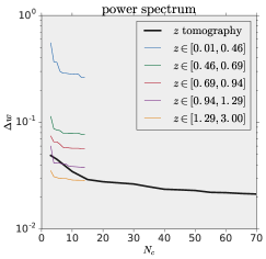
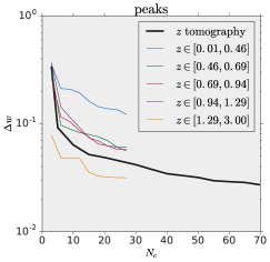
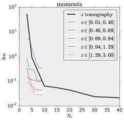
Figure 3: $1\sigma$ errors on $w$, marginalized over $(\Omega_{m},\sigma_{8})$, as a function of the number of the principal components $N_{c}$, using the power spectrum (top left), peak counts (top right) and moments (bottom). The thin colored lines refer to single redshift summary statistics, while the thick black line shows the case in which the joint redshift information is included.

In this section we present the main results of this work. Figure 3 shows the robustness of the dimensionality reduction technique we adopted for the three summary statistics considered, namely the convergence power spectrum $P^{\kappa\kappa}(\ell,\bar{z}_{b},\bar{z}_{b^{\prime}})$, peak counts $n_{\rm pk}(\nu,\bar{z}_{b})$ and moments $\boldsymbol{\mu}(\bar{z}_{b})$. To measure the power spectrum we chose 15 uniformly spaced multipole bands between $(\ell_{\rm min},\ell_{\rm max})=(200,2000)$. There are only 15 independent $(\bar{z}_{b},\bar{z}_{b^{\prime}})$ combinations (5 diagonal + 10 off-diagonal), which leads to a total of $N_{b}=15({\rm multipoles})\times 15({\rm redshift})=225$ power spectrum measurement bands, including cross redshift information. We bin the convergence peak counts in 30 uniformly spaced $\nu$ bins between $(\nu_{\rm min},\nu_{\rm max})=(-2,7)$, for a total of $N_{b}=30(\rm peak\,\,heights)\times 5({\rm redshift})=150$ measurement bands. The total size of the moments summary statistic vector is $N_{b}=9(\rm moments)\times 5(\rm redshift)=45$.

The forecast error bars on $w$ are calculated according to equation (15), where the covariance matrix $\mathbf{\hat{C}}$ and its inverse $\mathbf{\hat{\Psi}}$ have been estimated from $N_{r}=16000$ realizations of each summary statistic in the fiducial cosmology.

Figure 4 shows a comparison between the $w$ constraints obtained using single redshift bins, with and without PCA dimensionality reduction, and compares these single redshift constraints with the ones obtained using redshift tomography. When we calculate parameter inferences using the convergence power spectrum $P^{\kappa\kappa}$, we can cross check the results obtained with our simulations with the ones obtained with the analytical code NICAEA (Kilbinger et al., 2009). This code allows to predict the convergence power spectrum as a function of cosmological parameters $\mathbf{p}$, for an arbitrary galaxy redshift distribution $n(z)$. Parameter inferences can be obtained from the NICAEA predictions for $P^{\kappa\kappa}(\ell,z_{i},z_{j})$ (where $\{z_{i}\}$ are the centers of the redshift bins) using equation (15). To proceed in the calculations we approximate the $P^{\kappa\kappa}$ covariance matrix with the one one would obtain in the limit in which the $\kappa(\boldsymbol{\theta})$ field is Gaussian

$$\left\langle\delta\hat{P}_{\ell}(z_{1},z_{2})\delta\hat{P}_{\ell}(z_{3},z_{4})\right\rangle=\frac{P_{\ell}(z_{1},z_{3})P_{\ell}(z_{2},z_{4})+P_{\ell}(z_{1},z_{4})P_{\ell}(z_{2},z_{3})}{f_{\rm sky}\delta\ell_{\rm bin}(2\ell+1)}$$ (23)

where $P_{\ell}(z_{1},z_{2})$ is a shorthand for $P^{\kappa\kappa}(\ell,z_{1},z_{2})$, $\delta\hat{P}_{\ell}(z_{1},z_{2})=\hat{P}_{\ell}(z_{1},z_{2})-P_{\ell}(z_{1},z_{2})$ is the scatter in the $\hat{P}$ estimator, $\delta\ell_{\rm bin}$ is the width of the linearly spaced multipole bands and $f_{\rm sky}=\theta^{2}_{\rm FOV}/4\pi$ is the sky coverage fraction of one field of view. In this approximation the cross variance terms between different multipoles are assumed to be zero.

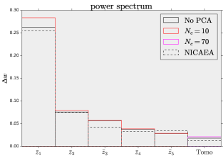
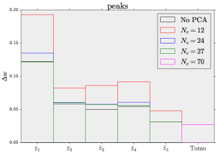
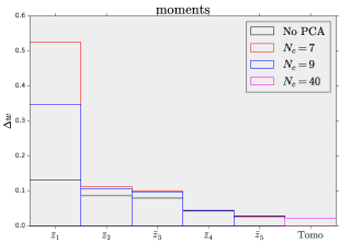
Figure 4: Comparison between single-redshift $w$ constraints (marginalized over $\Omega_{m}$ and $\sigma_{8}$) obtained without PCA (black bars) and with PCA (colored bars) as a function of the redshift bin $\bar{z}_{b}$. We show constraints obtained from the power spectrum (top left), peak counts (top right) and moments (bottom). Note the different scales on the vertical axis in the three different panels. The black dashed lines in the top left panel refer to parameter constraints on $w$ obtained with the public code NICAEA (Kilbinger et al., 2009), assuming a Gaussian covariance model for the power spectrum, as specified by equation (23).

Figure 5 shows the $1\sigma$ confidence contours on the $(\Omega_{m},w)$ doublet calculated from equation (15) after the PCA dimensionality reduction performed according to equation (20), for a variety of choices of statistic and $N_{c}$. We also show the improvements on the confidence contours when combining different summary statistics after the corresponding dimensionality reductions have been performed. The constraints in the $(\Omega_{m},w,\sigma_{8})$ parameter space for a variety of summary statistics are summarized in Tables 1 (weak lensing only) and 2 (with priors from Planck added).

Figure 6 shows the effect of ignoring photo-$z$ errors on parameter constraints. To evaluate this effect we construct different simulated observations, with and without photo-$z$ errors, and compare the results of the parameter fit according to equation (14). Using our simulation suite, we construct 20 simulated observations: the summary statistic in each observation is calculated by taking the mean of a random sample of $N_{\rm FOV}=1600$ realizations of the summary statistic in the fiducial cosmology (randomly chosen among the ensemble of $N_{r}=16000$ that are available in the ensemble). The estimated covariance matrix $\mathbf{\hat{C}}$ is scaled by a factor $N_{\rm FOV}$ to take into account the construction process of the simulated observations. This procedure allows us to forecast the results an LSST-like survey would obtain. We stress that, because of the small size of our simulation box the covariance estimate that we obtain is likely not accurate enough to produce constraints from LSST data. Full treatment of observables covariance matrices, along with larger $N$–body simulations and SSC effects will be investigated in future work.

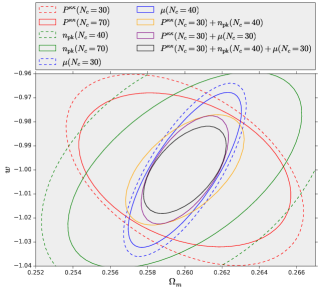
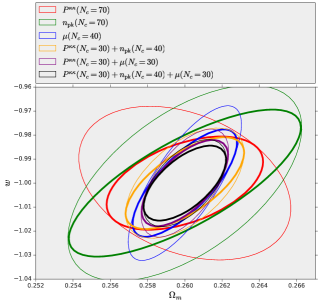
Figure 5: $1\sigma$ tomographic constraints on the $(\Omega_{m},w)$ parameter space, marginalized over $\sigma_{8}$, obtained using equation (15). The covariance matrix $\mathbf{\hat{C}}$ and its inverse $\mathbf{\hat{\Psi}}$ have been computed from $16000$ summary statistics realizations, and have been scaled by a factor $N_{\rm FOV}=1600$ to mimic the constraining power of an LSST-sized survey. The thick line ellipses in the right panel refer to $(\Omega_{m},w)$ obtained from the weak lensing statistics considered in this work, but subject to Planck priors as described in equation (22). The thin solid lines in the left and right panels are the same.

Statistic	$\Delta\Omega_{m}$	$\Delta w$	$\Delta\sigma_{8}$	$10^{6}{\rm Area}(\Omega_{m},w)$	$10^{9}{\rm Volume}$ $(\Omega_{m},w,\sigma_{8})$
Power spectrum ($\bar{z}_{5}$)	0.0222	0.0286	0.0298	632	654
Power spectrum (tomo)	0.0038	0.0213	0.0060	76	74
Peaks ($\bar{z}_{5}$)	0.0049	0.0316	0.0050	98	99
Peaks (tomo)	0.0042	0.0271	0.0043	93	122
Moments ($\bar{z}_{5}$)	0.0027	0.0276	0.0026	48	39
Moments (tomo)	0.0020	0.0214	0.0020	28	21
Power spectrum + peaks ($\bar{z}_{5}$)	0.0040	0.0209	0.0044	58	53
Power spectrum + peaks (tomo)	0.0021	0.0153	0.0026	27	26
Power spectrum + moments ($\bar{z}_{5}$)	0.0023	0.0190	0.0025	32	26
Power spectrum + moments (tomo)	0.0016	0.0150	0.0019	18	14
Power spectrum + peaks + moments ($\bar{z}_{5}$)	0.0020	0.0127	0.0024	21	17
Power spectrum + peaks + moments (tomo)	0.0015	0.0121	0.0018	14	11

Table 1: Constraints on the $(\Omega_{m},w,\sigma_{8})$ parameter triplet using different summary statistics and redshift information. Each column $(\Delta\Omega_{m},\Delta w,\Delta\sigma_{8})$ contains the 1$\sigma$ constraints on a particular parameter, marginalized over the other two. The last two columns contain respectively the area of the $(\Omega_{m},w)$ 68% confidence level ellipse (marginalized over $\sigma_{8}$) and the volume of the 68% confidence level ellipsoid in $(\Omega_{m},w,\sigma_{8})$ space, both calculated as the square root of the determinant of the relevant $\mathbf{\hat{\Sigma}}$ minors.

Statistic	$\Delta\Omega_{m}$	$\Delta w$	$\Delta\sigma_{8}$	$10^{6}{\rm Area}(\Omega_{m},w)$	$10^{9}{\rm Volume}$ $(\Omega_{m},w,\sigma_{8})$
Power spectrum ($\bar{z}_{5}$)	0.0076	0.0274	0.0084	94	96
Power spectrum (tomo)	0.0028	0.0129	0.0035	32	31
Peaks ($\bar{z}_{5}$)	0.0048	0.0237	0.0050	57	57
Peaks (tomo)	0.0041	0.0204	0.0042	55	70
Moments ($\bar{z}_{5}$)	0.0024	0.0172	0.0025	27	21
Moments (tomo)	0.0019	0.0149	0.0020	18	14
Power spectrum + peaks ($\bar{z}_{5}$)	0.0040	0.0184	0.0043	40	36
Power spectrum + peaks (tomo)	0.0021	0.0127	0.0025	20	19
Power spectrum + moments ($\bar{z}_{5}$)	0.0022	0.0145	0.0025	22	17
Power spectrum + moments (tomo)	0.0015	0.0120	0.0018	14	11
Power spectrum + peaks + moments ($\bar{z}_{5}$)	0.0019	0.0110	0.0023	16	13
Power spectrum + peaks + moments (tomo)	0.0015	0.0104	0.0018	12	9

Table 2: Constraints on the $(\Omega_{m},w,\sigma_{8})$ parameter triplet using different summary statistics and redshift information, including Fisher priors from Planck according to equation (22). Each column $(\Delta\Omega_{m},\Delta w,\Delta\sigma_{8})$ contains the 1$\sigma$ constraints on a particular parameter, marginalized over the other two. The last two columns contain respectively the area of the $(\Omega_{m},w)$ 68% confidence level ellipse (marginalized over $\sigma_{8}$) and the volume of the 68% confidence level ellipsoid in $(\Omega_{m},w,\sigma_{8})$ space, both calculated as the square root of the determinant of the relevant $\mathbf{\hat{\Sigma}}$ minors.

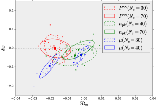
Figure 6: Distribution of parameter estimates in the $(\Omega_{m},w)$ parameter space using the power spectrum (red), peak counts (green) and moments (blue) to fit 20 LSST-like simulated observations. The parameter deviations $(\delta\Omega_{m},\delta w)$ are obtained comparing parameter estimates from equation (14) with and without photo-$z$ errors. The colored squares and the ellipses correspond to respectively to the mean and $1\sigma$ level of the $(\delta\Omega_{m},\delta w)$ distribution, assuming the latter is Gaussian.

IV Discussion

In this section we discuss our findings. Figure 3 shows that our dimensionality reduction technique is robust. In particular, for all the summary statistics we consider, a plateau in the $w$ error is reached for a sufficient high number of principal components $N_{c}$. We also see that for single redshift statistics, this plateau is reached for $\sim 5$ components for the power spectrum and the moments, and $\sim 10$ components for the peak counts. Moreover, Figure 4 shows that, at least for the four highest redshift bins $\{\bar{z}_{b}:b\geq 2\}$, most of the cosmological information contained in the full (pre-PCA) summary statistic vector can be captured with a limited number of principal components $N_{c}<N_{b}$. The minimum number of components necessary to capture most of the available information increases when including redshift tomography, and can reach $\sim 30$ for the power spectrum and moments and $\sim 40$ for the peak counts.

Figure 4 also clearly shows that, when considering a single redshift bin and a single summary statistic, most of the information on $w$ is contained in the highest redshift galaxies. PCA does not seem to capture all the information in the lowest redshift bin, even when enough components are included to reach the plateau in Figure 3. This can be attributed to the fact that PCA is not scale-invariant (Ivezić et al., 2014), because there is freedom in choosing the whitening scale in equation (18). Our choice of the whitening scale seems to affect significantly the first redshift bin, with the effect being mitigated for the highest redshift bins. The top left panel of Figure 4 also shows reasonable agreement between the results we obtain with our simulations and the ones we calculate with the analytical code NICAEA.

There are two possibilities for improving the constraints: the use of redshift tomography and the combination of different statistics. Table 1 shows that the area and volume of the $(\Omega_{m},w)$ ellipse and $(\Omega_{m},w,\sigma_{8})$ ellipsoid shrink by a factor of 8 when redshift tomography is added to the power spectrum, while the improvement is more modest for the remaining statistics (negligible for the peaks, and a factor of 2 for the moments). Combining the power spectrum and the peak counts in the highest redshift bin leads to a factor of 10 improvement in the $(\Omega_{m},w)$ and $(\Omega_{m},w,\sigma_{8})$ 68% confidence intervals, with tomography further shrinking the contours by an additional factor of 2. Combining the power spectrum and the moments in the highest redshift bin provides 20 times tighter constraints on $(\Omega_{m},w)$ and $(\Omega_{m},w,\sigma_{8})$, with tomography yielding an additional factor of 2 improvement. Table 1 also shows that power spectrum tomography can help breaking the degeneracy between $\Omega_{m}$ and $\sigma_{8}$. The same is not true for peaks and moments tomography, although combining these statistics with the power spectrum yields a factor of respectively 2 and 3 better constraints on $\Omega_{m}$ and $\sigma_{8}$.

Table 2 shows that parameter priors from Planck yield a factor of 6 improvement on the $(\Omega_{m},w)$ and $(\Omega_{m},w,\sigma_{8})$ 68% confidence intervals, even when a single redshift bin is considered. When the Planck priors in equation (22) are included, the improvements in constraints when adding redshift tomography or combining different statistics are more moderate. Tomography improves power spectrum constraints by a factor of 3. Adding moments improves by an additional factor of 2, and adding both moments and peaks improves by almost a factor of 3 over power spectrum tomography alone.

Figure 5 shows that peaks and moments contain cosmological information that is not contained in the power spectrum, because a similar improvement cannot be obtained by simply increasing the number of PCA components in the power spectrum dimensionality reduction procedure. This is consistent with previous work (see for example (Petri et al., 2015))

Figure 6 quantifies the effect of uncorrected photo-$z$ errors on the $(\Omega_{m},w)$ constraints. Because the stochastic nature of the observations, parameter values $\mathbf{\hat{p}}$ estimated from equation (14) are affected by statistical fluctuations. In Figure 6 we show 20 random draws from the probability distribution of $\delta\mathbf{\hat{p}}=\mathbf{\hat{p}}_{\rm photo-z}-\mathbf{\hat{p}}_{\rm no-photo-z}$. We can conclude that the $\mathbf{\hat{p}}$ estimator is biased if $\langle\delta\mathbf{\hat{p}}\rangle\neq 0$. Figure 6 clearly show that photo-$z$ errors cause parameter biases at more than $1\sigma$ significance level when using the power spectrum and the moments, while no bias is observed for the peak count statistic within its 68% confidence region. Peak histogram shapes are more robust to this kind of systematic effect since the peak locations are determined by the information coming from neighboring galaxies, while the photo-z errors have no spatial correlation. Photo-z errors are more likely to alter point estimates of the $\kappa$ distribution and larger scale correlations which affect the power spectrum.

We also observe that photo-$z$ errors bias the constraints in slightly different directions, leaving open the possibility of identifying and correcting this bias through self-calibration techniques.

V Conclusions

In this work we have studied cosmological parameter constraint forecasts for an LSST-like galaxy survey using the convergence power spectrum and a range of non-Gaussian statistics. We make use of redshift tomography to improve the constraints relative to their single-redshift counterparts. We also investigate the effects of uncorrected photo-$z$ systematic effects on the inferred cosmology. Our main findings can be summarized as follows:

• Principal Component analysis is a robust technique to keep the dimensionality of the parameter space under control and to avoid the numerical pitfalls explained in (Taylor et al., 2013; Dodelson and Schneider, 2013; Taylor and Joachimi, 2014) and more recently in (Petri et al., 2016). In particular, we find that only a few components (5-10) are necessary to characterize the cosmological information content in single redshift statistics, while more components (30-40) are necessary when tomography is included. Nevertheless we find that the number of required components $N_{c}$ is significantly smaller than the full summary statistic space dimensionality before performing PCA.

• When considering a single redshift bin, most of the cosmological information on $w$ is contained in high redshift galaxies. Constraints can be improved with redshift tomography or combining different non-Gaussian statistics with the power spectrum. The improvement originating from the combination of different statistics is attributed to the complementary information that non-Gaussian statistics carry, as a similar improvement cannot be obtained from a single statistic.

• Redshift tomography on the power spectrum shrinks the $(\Omega_{m},w)$ 68% confidence ellipse by a factor of 8; combining the peak counts with the power spectrum in the highest redshift bin leads to a factor of 10 better constraints, while adding the moments instead reduces the size of the $(\Omega_{m},w)$ ellipse by a factor of 20. When redshift tomography is added on top of these statistics combinations, an additional factor of 2 improvement is observed. Constraint improvements adding redshift tomography and combinations of different statistics are less dramatic when priors from CMB experiments are included in the analysis.

• Uncorrected photo-$z$ systematics can bias parameter constraints obtained from the power spectrum and the moments, but in slightly different parameter directions, leaving open possibilities of somewhat eliminating this bias via self-calibration.

This work explores the advantage of deep galaxy surveys such as LSST, which have access to shape and redshift information of high $z$ galaxies and provide valuable cosmological information on the dark energy equation of state. We also stress the fact that redshift tomography can in some cases provide more stringent constraints on parameters but, for this technique to be viable, accurate knowledge of galaxy redshifts is necessary. Future work needs to address the requirements for photometric measurements accuracy when using non-Gaussian statistics, as well as the self calibration techniques that can be used when different summary statistics are available in addition to the power spectrum.

References

- Schneider (2005) P. Schneider, ArXiv Astrophysics e-prints (2005), astro-ph/0509252 .
- Heymans et al. (2012) C. Heymans, L. Van Waerbeke, L. Miller, T. Erben, H. Hildebrandt, H. Hoekstra, T. D. Kitching, Y. Mellier, P. Simon, C. Bonnett, J. Coupon, L. Fu, J. Harnois Déraps, M. J. Hudson, M. Kilbinger, K. Kuijken, B. Rowe, T. Schrabback, E. Semboloni, E. van Uitert, S. Vafaei, and M. Velander, MNRAS 427, 146 (2012), arXiv:1210.0032 [astro-ph.CO] .
- Koekemoer et al. (2007) A. M. Koekemoer, H. Aussel, D. Calzetti, P. Capak, M. Giavalisco, J.-P. Kneib, A. Leauthaud, O. Le Fèvre, H. J. McCracken, R. Massey, B. Mobasher, J. Rhodes, N. Scoville, and P. L. Shopbell, ApJS 172, 196 (2007), astro-ph/0703095 .
- Gruen et al. (2016) D. Gruen, O. Friedrich, A. Amara, D. Bacon, C. Bonnett, W. Hartley, B. Jain, M. Jarvis, T. Kacprzak, E. Krause, A. Mana, E. Rozo, E. S. Rykoff, S. Seitz, E. Sheldon, M. A. Troxel, V. Vikram, T. M. C. Abbott, F. B. Abdalla, S. Allam, R. Armstrong, M. Banerji, A. H. Bauer, M. R. Becker, A. Benoit-Lévy, G. M. Bernstein, R. A. Bernstein, E. Bertin, S. L. Bridle, D. Brooks, E. Buckley-Geer, D. L. Burke, D. Capozzi, A. Carnero Rosell, M. Carrasco Kind, J. Carretero, M. Crocce, C. E. Cunha, C. B. D’Andrea, L. N. da Costa, D. L. DePoy, S. Desai, H. T. Diehl, J. P. Dietrich, P. Doel, T. F. Eifler, A. F. Neto, E. Fernandez, B. Flaugher, P. Fosalba, J. Frieman, D. W. Gerdes, R. A. Gruendl, G. Gutierrez, K. Honscheid, D. J. James, K. Kuehn, N. Kuropatkin, O. Lahav, T. S. Li, M. Lima, M. A. G. Maia, M. March, P. Martini, P. Melchior, C. J. Miller, R. Miquel, J. J. Mohr, B. Nord, R. Ogando, A. A. Plazas, K. Reil, A. K. Romer, A. Roodman, M. Sako, E. Sanchez, V. Scarpine, M. Schubnell, I. Sevilla-Noarbe, R. C. Smith, M. Soares-Santos, F. Sobreira, E. Suchyta, M. E. C. Swanson, G. Tarle, J. Thaler, D. Thomas, A. R. Walker, R. H. Wechsler, J. Weller, Y. Zhang, and J. Zuntz, MNRAS 455, 3367 (2016), arXiv:1507.05090 .
- LSST Dark Energy Science Collaboration (2012) LSST Dark Energy Science Collaboration, ArXiv e-prints (2012), arXiv:1211.0310 [astro-ph.CO] .
- Spergel et al. (2015) D. Spergel, N. Gehrels, C. Baltay, D. Bennett, J. Breckinridge, M. Donahue, A. Dressler, B. S. Gaudi, T. Greene, O. Guyon, C. Hirata, J. Kalirai, N. J. Kasdin, B. Macintosh, W. Moos, S. Perlmutter, M. Postman, B. Rauscher, J. Rhodes, Y. Wang, D. Weinberg, D. Benford, M. Hudson, W.-S. Jeong, Y. Mellier, W. Traub, T. Yamada, P. Capak, J. Colbert, D. Masters, M. Penny, D. Savransky, D. Stern, N. Zimmerman, R. Barry, L. Bartusek, K. Carpenter, E. Cheng, D. Content, F. Dekens, R. Demers, K. Grady, C. Jackson, G. Kuan, J. Kruk, M. Melton, B. Nemati, B. Parvin, I. Poberezhskiy, C. Peddie, J. Ruffa, J. K. Wallace, A. Whipple, E. Wollack, and F. Zhao, ArXiv e-prints (2015), arXiv:1503.03757 [astro-ph.IM] .
- Amiaux et al. (2012) J. Amiaux, R. Scaramella, Y. Mellier, B. Altieri, C. Burigana, A. Da Silva, P. Gomez, J. Hoar, R. Laureijs, E. Maiorano, D. Magalhães Oliveira, F. Renk, G. Saavedra Criado, I. Tereno, J. L. Auguères, J. Brinchmann, M. Cropper, L. Duvet, A. Ealet, P. Franzetti, B. Garilli, P. Gondoin, L. Guzzo, H. Hoekstra, R. Holmes, K. Jahnke, T. Kitching, M. Meneghetti, W. Percival, and S. Warren, in Society of Photo-Optical Instrumentation Engineers (SPIE) Conference Series, Society of Photo-Optical Instrumentation Engineers (SPIE) Conference Series, Vol. 8442 (2012) p. 84420Z, arXiv:1209.2228 [astro-ph.IM] .
- Kratochvil et al. (2012) J. M. Kratochvil, E. A. Lim, S. Wang, Z. Haiman, M. May, and K. Huffenberger, Phys. Rev. D 85, 103513 (2012), arXiv:1109.6334 [astro-ph.CO] .
- Yang et al. (2011) X. Yang, J. M. Kratochvil, S. Wang, E. A. Lim, Z. Haiman, and M. May, Phys. Rev. D 84, 043529 (2011), arXiv:1109.6333 .
- Marian et al. (2009) L. Marian, R. E. Smith, and G. M. Bernstein, ApJ 698, L33 (2009), arXiv:0811.1991 .
- Takada and Jain (2002) M. Takada and B. Jain, MNRAS 337, 875 (2002), astro-ph/0205055 .
- Takada and Jain (2003) M. Takada and B. Jain, MNRAS 344, 857 (2003), astro-ph/0304034 .
- Takada and Jain (2004) M. Takada and B. Jain, MNRAS 348, 897 (2004), astro-ph/0310125 .
- Bergé et al. (2010) J. Bergé, A. Amara, and A. Réfrégier, ApJ 712, 992 (2010), arXiv:0909.0529 .
- Dietrich and Hartlap (2010) J. P. Dietrich and J. Hartlap, MNRAS 402, 1049 (2010), arXiv:0906.3512 .
- Song and Knox (2004) Y.-S. Song and L. Knox, Phys. Rev. D 70, 063510 (2004), arXiv:astro-ph/0312175 .
- Fang and Haiman (2007) W. Fang and Z. Haiman, Phys. Rev. D 75, 043010 (2007), astro-ph/0612187 .
- Huterer, D. and Takada, M. and Bernstein, G. and Jain, B. (2006) Huterer, D. and Takada, M. and Bernstein, G. and Jain, B., MNRAS 366, 101 (2006), astro-ph/0506030 .
- Martinet et al. (2015) N. Martinet, J. G. Bartlett, A. Kiessling, and B. Sartoris, A&A 581, A101 (2015), arXiv:1506.02192 .
- Hinshaw et al. (2013) G. Hinshaw, D. Larson, E. Komatsu, D. N. Spergel, C. L. Bennett, J. Dunkley, M. R. Nolta, M. Halpern, R. S. Hill, N. Odegard, L. Page, K. M. Smith, J. L. Weiland, B. Gold, N. Jarosik, A. Kogut, M. Limon, S. S. Meyer, G. S. Tucker, E. Wollack, and E. L. Wright, ApJS 208, 19 (2013), arXiv:1212.5226 .
- Planck Collaboration et al. (2015) Planck Collaboration, P. A. R. Ade, N. Aghanim, M. Arnaud, M. Ashdown, J. Aumont, C. Baccigalupi, A. J. Banday, R. B. Barreiro, J. G. Bartlett, and et al., ArXiv e-prints (2015), arXiv:1502.01589 .
- Springel (2005) V. Springel, MNRAS 364, 1105 (2005), astro-ph/0505010 .
- Sato et al. (2009) M. Sato, T. Hamana, R. Takahashi, M. Takada, N. Yoshida, T. Matsubara, and N. Sugiyama, ApJ 701, 945 (2009), arXiv:0906.2237 [astro-ph.CO] .
- Takada and Hu (2013) M. Takada and W. Hu, Phys. Rev. D 87, 123504 (2013), arXiv:1302.6994 [astro-ph.CO] .
- Mohammed et al. (2016) I. Mohammed, U. Seljak, and Z. Vlah, ArXiv e-prints (2016), arXiv:1607.00043 .
- Heitmann et al. (2015) K. Heitmann, N. Frontiere, C. Sewell, S. Habib, A. Pope, H. Finkel, S. Rizzi, J. Insley, and S. Bhattacharya, ApJS 219, 34 (2015), arXiv:1411.3396 .
- Habib et al. (2016) S. Habib, A. Pope, H. Finkel, N. Frontiere, K. Heitmann, D. Daniel, P. Fasel, V. Morozov, G. Zagaris, T. Peterka, V. Vishwanath, Z. Lukić, S. Sehrish, and W.-k. Liao, 42, 49 (2016), arXiv:1410.2805 [astro-ph.IM] .
- Jain et al. (2000) B. Jain, U. Seljak, and S. White, ApJ 530, 547 (2000), astro-ph/9901191 .
- Hilbert et al. (2009) S. Hilbert, J. Hartlap, S. D. M. White, and P. Schneider, A&A 499, 31 (2009), arXiv:0809.5035 .
- Petri (2016a) A. Petri, “LensTools: Weak Lensing computing tools,” Astrophysics Source Code Library (2016a), ascl:1602.009 .
- Petri (2016b) A. Petri, Astronomy and Computing 17, 73 (2016b), arXiv:1606.01903 .
- Petri et al. (2016) A. Petri, Z. Haiman, and M. May, Phys. Rev. D 93, 063524 (2016).
- Petri et al. (2015) A. Petri, J. Liu, Z. Haiman, M. May, L. Hui, and J. M. Kratochvil, Phys. Rev. D 91, 103511 (2015), arXiv:1503.06214 .
- Liu et al. (2015) J. Liu, A. Petri, Z. Haiman, L. Hui, J. M. Kratochvil, and M. May, Phys. Rev. D 91, 063507 (2015), arXiv:1412.0757 .
- Zhan (2006) H. Zhan, JCAP 8, 008 (2006), astro-ph/0605696 .
- LSST Science Collaboration et al. (2009) LSST Science Collaboration, P. A. Abell, J. Allison, S. F. Anderson, J. R. Andrew, J. R. P. Angel, L. Armus, D. Arnett, S. J. Asztalos, T. S. Axelrod, and et al., ArXiv e-prints (2009), arXiv:0912.0201 [astro-ph.IM] .
- Casarini et al. (2015) L. Casarini, O. F. Piattella, S. A. Bonometto, and M. Mezzetti, ApJ 812, 16 (2015), arXiv:1406.5374 .
- Matsubara (2010) T. Matsubara, Phys. Rev. D 81, 083505 (2010), arXiv:1001.2321 [astro-ph.CO] .
- Munshi et al. (2012) D. Munshi, L. van Waerbeke, J. Smidt, and P. Coles, MNRAS 419, 536 (2012), arXiv:1103.1876 [astro-ph.CO] .
- Petri et al. (2013) A. Petri, Z. Haiman, L. Hui, M. May, and J. M. Kratochvil, Phys. Rev. D 88, 123002 (2013), arXiv:1309.4460 .
- Ivezić et al. (2014) Ž. Ivezić, A. Connolly, J. Vanderplas, and A. Gray, Statistics, Data Mining and Machine Learning in Astronomy (Princeton University Press, 2014).
- Hartlap et al. (2007) J. Hartlap, P. Simon, and P. Schneider, A&A 464, 399 (2007), arXiv:astro-ph/0608064 .
- Taylor et al. (2013) A. Taylor, B. Joachimi, and T. Kitching, MNRAS 432, 1928 (2013), arXiv:1212.4359 .
- Taylor and Joachimi (2014) A. Taylor and B. Joachimi, MNRAS 442, 2728 (2014), arXiv:1402.6983 .
- Note (1) The archive we used is located http://pla.esac.esa.int/pla/; we used the MCMC chains contained in the base_w/plikHM_TT_lowTEB directory, labeled as base_w_plikHM_TT_lowTEB_[1-4].txt.
- Kilbinger et al. (2009) M. Kilbinger, K. Benabed, J. Guy, P. Astier, I. Tereno, L. Fu, D. Wraith, J. Coupon, Y. Mellier, C. Balland, F. R. Bouchet, T. Hamana, D. Hardin, H. J. McCracken, R. Pain, N. Regnault, M. Schultheis, and H. Yahagi, A&A 497, 677 (2009), arXiv:0810.5129 .
- Dodelson and Schneider (2013) S. Dodelson and M. D. Schneider, Phys. Rev. D 88, 063537 (2013), arXiv:1304.2593 [astro-ph.CO] .