The Resistance Perturbation Distance:
A Metric for the Analysis of Dynamic Networks

Abstract

To quantify the fundamental evolution of time-varying networks, and detect abnormal behavior, one needs a notion of temporal difference that captures significant organizational changes between two successive instants. In this work, we propose a family of distances that can be tuned to quantify structural changes occurring on a graph at different scales: from the local scale formed by the neighbors of each vertex, to the largest scale that quantifies the connections between clusters, or communities. Our approach results in the definition of a true distance, and not merely a notion of similarity. We propose fast (linear in the number of edges) randomized algorithms that can quickly compute an approximation to the graph metric. The third contribution involves a fast algorithm to increase the robustness of a network by optimally decreasing the Kirchhoff index. Finally, we conduct several experiments on synthetic graphs and real networks, and we demonstrate that we can detect configurational changes that are directly related to the hidden variables governing the evolution of dynamic networks.

1 Introduction

Many complex systems are well represented as graphs or networks, with the agents represented as vertices and edges symbolizing relationships or similarities between them. In many instances, the relationships between vertices evolve as a function of time: edges may appear and disappear, the weights along the edges may change. The study of such dynamic graphs often involves the identification of patterns that couple changes in the network topology with the latent dynamical processes that drive the evolution of the connectivity of the network [2, 24, 30, 31, 42].

To quantify the temporal and structural evolution of time-varying networks, and detect abnormal behavior, one needs a notion of temporal difference that captures significant configurational changes between two successive instants. The design of similarity measures for the pairwise comparison of graphs [45] is therefore of fundamental importance.

Because we are interested in detecting changes between two successive instants, we focus on the problem of measuring the distance between two graphs on the same vertex set, with known vertex correspondence (see Fig. 1). We note that determining whether two graphs are isomorphic under a permutation of the vertex labels is a combinatorially hard problem (e.g., [35], and references therein, but see the recent results [3]). Several notion of similarities (e.g., [8, 36, 29], and references therein) have been proposed. Unlike a true metric, a similarity merely provides a notion of resemblance. Most approaches rely on the construction of a feature vector that provides a signature of the graph characteristics; the respective feature vectors of the two graphs are then compared using some norm, or distance. A similarity function is typically not injective (two graphs can be perfectly similar without being the same), and rarely satisfies the triangular inequality.

Instead of comparing two feature vectors, several researchers (e.g., [1, 9, 11, 4, 19, 43, 52] and references therein) have proposed to use a kernel function. This approach offers the same advantage as the computation of a similarity:

Figure 1: Dynamic graph $G^{(t)}$ at time $t$ (left) and $t+1$ (right)

the isomorphism problem need not be solved. Unfortunately, the kernels do not define proper metrics, and we are left with a weaker notion of similarity.

Several distances between two graphs with the same size have been proposed (e.g., [7, 11], and references therein). As detailed in section 3.2, we argue that existing distances either fail to capture a notion of structural similarity, or lead to algorithms that have a high computational complexity.

1.1 Contribution and Organization of the Paper

The contributions of this work are threefold. First, we propose a family of distances that can be tuned to quantify configurational changes that occur on a graph at different scales: from the local scale formed by the local neighbors of each vertex, to the largest scale that quantifies the connections between clusters, or communities. Our approach results in the definition of a true distance, and not merely a notion of similarity. The second contribution encompasses fast computational algorithms to evaluate the metrics developed in the first part. We developed fast (linear in the number of edges) randomized algorithms that can quickly compute an approximation to the graph metric. The third contribution involves fast algorithms to increase the robustness of a network by optimally decreasing the Kirchhoff index. Finally, we conduct several experiments on synthetic and real dynamic networks, and we demonstrate that the resistance perturbation distance can detect the significant changes in the hidden latent variables that control the network dynamics.

The remainder of this paper is organized as follows. In the next section we introduce the main mathematical concepts and corresponding nomenclature. In section 3 we formally define the problem and review the existing literature. In section 4 we propose a novel framework for constructing graph distances; we focus the rest of the paper on the resistance perturbation distance, which is defined in section 5. In section 6, we study simple perturbations of several prototypical graphs for which the resistance perturbation distance can be computed analytically. Fast randomized algorithms are described in section 7. The optimization of the robustness of a network, based on optimally decreasing the Kirchhoff index, is described in section 8. In section 9, we use the resistance perturbation metric to detect significant changes in synthetic and real dynamic networks. We conclude in Section 10 with a discussion on future work. Some technical details and proofs are left aside in the Appendix. A list of the main notations used in the paper is provided in section 11.

2 Preliminaries and Notation

We introduce in this section the main concepts and associated nomenclature.

We denote by $\bm{e}_{i}$ the $i^{\text{th}}$ vector of the canonical basis in $\mathbb{R}^{n}$. The space of matrices of size $n\times m$ with entries in $\mathbb{R}$ is denoted by $\bm{M}_{n\times m}$; to alleviate notations we write $\bm{M}_{n}$ to denote $\bm{M}_{n\times n}$.

We denote by $G=(V,E,w)$ an undirected weighted graph with a vertex set $V=\{1,\ldots,n\}$, an edge set $E$, and a symmetric weight function $w$ that quantifies the similarity between any two vertices $i$ and $j$. In this work, we use the terms graph and network exchangeably.

The weighted adjacency matrix, $\bm{A}\in\bm{M}_{n}$, is given by

$$A_{ij}=A_{ji}=\begin{cases}w_{e}&\text{if the edge}\;e=[i,j]\in E,\\ 0&\text{otherwise.}\end{cases}$$ (1)

For simplicity, we will always assume $G$ is connected and does not contain any self-loops. We further define the combinatorial Laplacian matrix,

$$\bm{L}=\bm{D}-\bm{A},$$ (2)

where the degree matrix $\bm{D}$ is the diagonal matrix of vertex degrees,

$$D_{ii}=\sum_{j=1}^{n}A_{ij}.$$

The matrix $\bm{L}$ is symmetric and positive semi-definite. We denote by $\bm{\phi}_{k}$ the $k^{\text{th}}$ eigenvector of $\bm{L}$ corresponding to $\lambda_{k}$, with $0=\lambda_{1}<\lambda_{2}\leq\ldots\leq\lambda_{n}$. We can write $\bm{L}$ in terms of its spectral decomposition,

$$\bm{L}=\sum_{k=2}^{n}\lambda_{k}\bm{\phi}_{k}\bm{\phi}_{k}^{T}.$$ (3)

$\bm{L}^{\dagger}$ denotes the Moore-Penrose pseudoinverse of $\bm{L}$. Because $\bm{L}$ is symmetric, $\bm{L}^{\dagger}$ is also symmetric. The pseudoinverse is easily formulated from the spectral decomposition of $\bm{L}$,

$$\bm{L}^{\dagger}=\sum_{k=2}^{n}\frac{1}{\lambda_{k}}\bm{\phi}_{k}\bm{\phi}_{k}^{T}.$$ (4)

We can also express $\bm{L}^{\dagger}$ in terms of the inverse of $\bm{L}+\frac{1}{n}\bm{J}$, which is full-rank,

$$\bm{L}^{\dagger}=\left(\bm{L}+\frac{1}{n}\bm{J}\right)^{-1}-\frac{1}{n}\bm{J},$$ (5)

where

$$\bm{J}=\bm{1}\bm{1}^{T},\;\text{with}\quad\bm{1}^{T}=\begin{bmatrix}1&1&\cdots&\end{bmatrix}.$$ (6)

For the purpose of defining a concept of gradient on the graph, we assign an (arbitrary) orientation to each edge $e$. With this orientation, we define a notion of gradient, captured by the signed edge incidence matrix, $\bm{B}\in\bm{M}_{m\times n}$,

$$B_{ei}=\begin{cases}1&\text{if vertex $i$ is at the head of $e$,}\\ -1&\text{if vertex $i$ is at the tail of $e$,}\\ 0&\text{otherwise.}\end{cases}$$ (7)

We define the diagonal edge weight matrix $\bm{{d\mspace{-1.0mu}A}}\in\bm{M}_{m\times n}$ with diagonal entries $\bm{{d\mspace{-1.0mu}A}}_{ee}=w_{e}$. The (gradient) edge incidence matrix can be used to express the combinatorial Laplacian matrix as

$$\bm{L}=\bm{B}^{T}\bm{{d\mspace{-1.0mu}A}}\bm{B}.$$ (8)

In this paper we are concerned with two undirected weighted graphs $G^{(1)}$ and $G^{(2)}$ with a common vertex set $V=\{1,\ldots,n\}$, two edge sets $E^{(1)}$ and $E^{(2)}$, and two symmetric weight functions $w^{(1)}$ and $w^{(2)}$. We denote by $\bm{A}^{(1)}$ and $\bm{A}^{(2)}$ the corresponding weighted adjacency matrices.

3 Statement of the Problem and Related Work

Inspired by the work of Koutra et al. [29], we propose to characterize distances between graphs using a set of axioms and principles. After defining these axioms and principles, we use these to review the existing literature on graph distance and similarity.

3.1 Metrics Between Graphs: an Axiomatic Definition

Axiom 1 (Definition of a Distance)

A distance on a space of graphs should meet all the conditions of a distance: non-negativity, identity, symmetry, and subadditivity.

The set of axioms in Koutra et al. [29] are somewhat similar to our single axiom, given the translation of a distance into a similarity measure. Our axiom is stronger in that it also implies the triangle inequality, in addition to symmetry and identity (the first two axioms in [29]).

We note that Axiom 3 from Koutra et al. [29] is the Zero property:
$\text{sim}(G^{(1)},G^{(2)})\rightarrow 0$ as $n\rightarrow\infty$, if $G^{(1)}$ is the complete graph and $G^{(2)}$ is the empty graph. As explained in Remark 3, the zero property holds in our case: if $G^{(2)}$ is obtained by disconnecting $G^{(1)}$, then our distance goes to infinity; in other words the similarity goes to zero.

In addition to the above axiom, we argue that a useful distance should obey the following the four principles proposed by Koutra et al. [29].

Principle 1 (Edge Importance)

Changes that create disconnected components should be penalized more than changes that maintain the connectivity properties of the graphs.

Principle 2 (Weight Awareness)

In weighted graphs, the larger the weight of the removed edge is, the greater the impact on the distance should be.

Principle 3 (Edge-“Submodularity”)

A specific change is more important in a graph with few edges than in a much denser, but equally sized graph.

Principle 4 (Focus Awareness)

Random changes in graphs are less important than targeted changes of the same extent.

The first three principles are intuitive and self-explanatory. The principle of focus awareness requires some interpretation. Koutra et al. [29] test for focus awareness by either removing all edges connected to a vertex (a targeted change) or randomly removing the same number of edges from the whole graph (a random change of the same extent). In most applications, the targeted removal of all edges connecting a single vertex would be viewed as a more significant change to the network topology compared with most realizations of random edge removal. An ideal distance should account for the relative importance of these types of changes.

We propose an alternative interpretation of the “focus awareness” principle. We first observe that edges can be partitioned in terms of their “functionality” in the network. In this work, the notion of functionality is measured in terms of connectivity, and is quantified with the concept of effective resistance. Now, if we consider the distribution of effective resistances across all edges in $E$, some edges will contribute to rare events because they have very large effective resistance. We argue that such edges are unlikely to be removed by a random selection of edges in the network. In other words, a targeted change would correspond to a perturbation of these rare edges with very high effective resistance. Our definition of focus awareness recovers the intuitive notion introduced by Koutra et al. [29]. This point is further discussed in section 10.

Adherence to the axioms and principles does not imply that a distance will be useful in practice. A distance must also be computable. Modern applications require algorithms to compute or approximate the distance in nearly linear time in the number of edges.

3.2 Existing Notions of Similarities Between Graphs

Unlike a true metric that satisfies the three axioms of a metric, similarities are merely providing a notion of resemblance. This approach relies on the construction of a feature vector that provides a signature of the graph characteristics; the respective feature vectors of the two graphs are then compared using some norm, or distance (e.g., [8, 29, 36], and references therein). The similarity function is typically not injective (two graphs can be perfectly similar without being the same), and rarely satisfies the triangular inequality. The authors in [29] offer a list of properties that a “good” similarity should obey. They define the DeltaCon₀ similarity as follows,

$$\text{sim}_{\text{DC}_{0}}\left(G^{(1)},G^{(2)}\right)=\frac{1}{1+{d_{\text{rootED}}\left({G^{(1)}},{G^{(2)}}\right)}},$$ (9)

where the root Euclidean distance is defined as

$${d_{\text{rootED}}\left({G^{(1)}},{G^{(2)}}\right)}=\left\{\sum_{i,j=1}^{n}\left(\sqrt{{\bm{S}}^{(1)}_{ij}}-\sqrt{{\bm{S}}^{(2)}_{ij}}\right)^{2}\right\}^{1/2}\mspace{-24.0mu},$$ (10)

and where ${\bm{S}}^{(i)}$ is the fast belief propagation matrix defined by

$${\bm{S}}^{(i)}=\left[\bm{I}+\varepsilon^{2}\bm{D}^{(i)}-\varepsilon{\bm{A}}^{(i)}\right]^{-1}\mspace{-24.0mu},$$ (11)

and $\varepsilon=1/(1+\max_{i}D_{ii})$. To gain some intuition about the role of the fast belief propagation matrix $\bm{S}$ , we assume $\varepsilon\ll 1$, and drop the term $\varepsilon^{2}\bm{D}$ in $\bm{S}$ to arrive at

$$\bm{S}\approx\left(\bm{I}-\varepsilon\bm{A}\right)^{-1}=\bm{I}+\varepsilon\bm{A}+\varepsilon^{2}{\bm{A}}^{2}+\varepsilon^{3}{\bm{A}}^{3}+\ldots.$$ (12)

In the unweighted case, $A^{k}_{ij}$ is the count of paths of length $k$ between vertices $i$ and $j$. In the weighted case, $A^{k}_{ij}$ is the sum, over all paths of length $k$ between vertices $i$ and $j$, of the product of the weights along the corresponding paths. We conclude that $\bm{S}$ encapsulates information about the connectivity between vertices at all scales (with longer paths having a reduced impact).

We provide in A a detailed analysis of the DeltaCon₀ distance that uncovers unexpected behavior. Our analysis is based on a single-edge

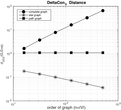
Figure 2: Experimental scaling of the DeltaCon₀ similarity (left) and the resistance perturbation distance (right) for single edge perturbation of simple graphs.

perturbation of several simple graphs, where the DeltaCon₀ distance between the original and perturbed graphs can be computed analytically.

In the case of the complete graph, $K_{n}$, the root Euclidean distance created by the perturbation grows with $n=|V|$,

$${d_{\text{rootED}}\left({K_{n}},{K_{n}+{\Delta w_{kl}})}\right)}=\left|\frac{1}{\sqrt{2}}-\frac{1}{\sqrt{2+{\Delta w_{kl}}}}\right\rvert n+{\cal O}\left(1\right).$$ (13)

However, in the case of the much sparser star graph, $S_{n}$, the root Euclidean distance decays with $n=|V|$,

$${d_{\text{rootED}}\left({S_{n}},{S_{n}+{\Delta w_{kl}}}\right)}=\frac{\sqrt{2{\Delta w_{kl}}}}{\sqrt{n}}-\frac{\sqrt{2}}{n}+{\cal O}\left(1/n^{3/2}\right).$$ (14)

These leading-order analyses are confirmed experimentally in Fig. 2, where we compare the DeltaCon₀ similarity with the resistance perturbation presented in this paper.

We can interpret these results in terms of the graph density. The density of the complete graph $K_{n}$, as measured by the average degree ${\overline{d_{n}}}$, is $n-1$, whereas the densities of the star $S_{n}$ and path $P_{n}$ graphs are $2(1-1/n)$ and $1$ respectively,

$${\overline{d_{n}}}(P_{n})=1<{\overline{d_{n}}}(S_{n})=2\left(1-1/n\right)<{\overline{d_{n}}}(K_{n})=n-1,\quad n\geq 3.$$ (15)

The DeltaCon distances for a single edge perturbation are ordered as follows,

$$\begin{split}{d_{\text{rootED}}\left({S_{n}},{S_{n}+{\Delta w_{kl}}}\right)}={\Theta}\left(\displaystyle\frac{1}{\sqrt{n}}\right)&<{d_{\text{rootED}}\left({P_{n}},{P_{n}+{\Delta w_{kl}}}\right)}={\Theta}\left(1\right)\\ &<{d_{\text{rootED}}\left({K_{n}},{K_{n}+{\Delta w_{kl}}}\right)}={\Theta}\left(n\right),\end{split}$$ (16)

while the RP distances for the respective graphs are ordered as follows,

$$\begin{split}\operatorname{d_{\operatorname{rp}1}}\left(K_{n},K_{n}+{\Delta w_{kl}}\right)={\Theta}\left(\displaystyle\frac{1}{n}\right)&<\operatorname{d_{\operatorname{rp}1}}\left(S_{n},S_{n}+{\Delta w_{kl}}\right)={\Theta}\left(n\right)\\ &<\operatorname{d_{\operatorname{rp}1}}\left(P_{n},P_{n}+{\Delta w_{kl}}\right)={\Theta}\left(n^{3}\right).\end{split}$$ (17)

We conclude that, on these three graphs, the RP distance for a single edge perturbation decreases as a function of the graph density, which is consistent with Principle 3 from Koutra et al. [29], which asserts that “A specific change is more important in a graph with few edges than in a much denser, but equally sized graph.”

The ordering of the DeltaCon distances is not exactly the reverse of the ordering of the RP-distances. Nevertheless, when comparing the complete graph to either the star, or the path graphs, we conclude that the DeltaCon distance for a single edge perturbation increases as a function of the graph density, which is inconsistent with Principle 3.

Indeed, a principled distance should ascribe greater significance to changing an edge weight in the star graph (a sparser graph in which each edge is more important) relative to the complete graph (a dense graph in which no single edge is crucial to the overall connectivity).

When comparing the star to the path, we note that DeltaCon respects Principle 3. Because both the star and the path graphs have a constant density, we find this comparison to be less of a concern. We complement our theoretical analysis of DeltaCon₀ with an experimental evaluation conducted in Section 9.

In the context of the analysis of dynamic graphs, the authors in [50] describe an algorithm to localize edges that most significantly contribute to dynamical structural changes. To tackle this question, the authors define the following distance to quantify structural changes as the graph $G^{(n)}$ evolves to $G^{(n+1)}$,

$$d_{\text{CAD}}(G^{(n)},G^{(n+1)})=\mspace{-32.0mu}\sum_{(u,v)\in F\subseteq E^{(n)}}\mspace{-32.0mu}\left|A^{(n+1)}(u,v)-A^{(n)}(u,v)\right|\left|\kappa^{(n+1)}(u,v)-\kappa^{(n)}(u,v)\right|,$$ (18)

where $F$ is a subset of the edge set $E^{(n)}$ of the graph $G^{(n)}$, and $\kappa^{(n)}_{u,v}$ is the commute time between vertices $u$ and $v$ in the graph $G^{(n)}$ (see Definition 26).

The authors in [50] propose to minimize this distance to identify the maximal “core” subset of edges $F$ that contribute to the least structural changes between time $n$ and $n+1$. The complement of the core set $F$ consists of edges that trigger large structural changes.

While the goal of our work is quite different from that of [50], our notion of effective resistance, defined in (28), is indeed similar to the distance (18). As explained in section 5.1, the commute time is – up to a renormalization by the volume of the graph $m=|E^{(n)}|$ – the same as the effective resistance.

Because of the presence of the term $\left|A^{(n+1)}(u,v)-A^{(n)}(u,v)\right|$, the distance $d_{\text{CAD}}$ does not satisfy the triangle inequality. We suspect that $d_{\text{CAD}}$ is not injective. An increase (decrease) in the commute time $\kappa_{uv}$ throughout the graph could in principle be cancelled by a corresponding increase (decrease) in the volume $m$, to keep the effective resistance the same (see (27)). This argument is not in contradiction with the Rayleigh’s Monotonicity Principle that only applies to effective resistance, and not the commute time.

Because of the similarity between the distance $d_{\text{CAD}}$ and the resistance perturbation distance, we evaluated $d_{\text{CAD}}$ in all experiments conducted in section 9.

Another similarity that captures the geometry of the graph at all scale is provided by the spectral similarity which quantifies the distance between the respective spectra $\{\lambda^{(1)}_{i}\}_{i=1}^{n}$ and $\{\lambda^{(2)}_{i}\}_{i=1}^{n}$ of $G^{(1)}$ and $G^{(2)}$ The spectra can be computed from the adjacency, Laplacian, or normalized Laplacian matrices [10, 38, 55]. The spectral similarity is defined by

$$d_{\lambda}\left(G^{(1)},G^{(2)}\right)=\sqrt{\displaystyle\sum_{i=1}^{n}\left(\lambda^{(1)}_{i}-\lambda^{(2)}_{i}\right)^{2}}.$$

The existence of iso-spectral graphs prevents $d_{\lambda}$ to be a distance, since
$d_{\lambda}\left(G^{(1)},G^{(2)}\right)=0$ does not necessarily imply that $G^{(1)}=G^{(2)}$. In addition, the spectral methods are costly since they require computation of the full graph spectrum.

Signature similarity is another method considered in Koutra et al. [29]. The signature similarity compares two graphs by first computing a large number of features from the two graphs. These features are then projected onto a random lower-dimensional feature space within which the similarity between the two graphs is computed. This method was found to be the best performing method in Papadimitriou et al. [36]. Unfortunately, Koutra et al. [29] proved that the signature similarity, along with the graph edit distance, and all variants of the $\lambda$-distance fail to conform to Principles 1 and 3.

Other notions of similarity, which do not necessarily define a proper distance, can be defined. For example, Spielman and Teng [49] (see also [6]) introduced another notion of spectral similarity. Two graphs $G^{(1)}$ and $G^{(2)}$, with Laplacians $\bm{L}^{(1)}$ and $\bm{L}^{(2)}$, on the same vertex set $V$ are said to be $\sigma$-spectrally similar if [49],

$$\frac{1}{\sigma}\;\bm{x}^{T}\bm{L}^{(2)}\mspace{-2.0mu}\bm{x}\leq\bm{x}^{T}\bm{L}^{(1)}\mspace{-2.0mu}\bm{x}\leq\sigma\;\bm{x}^{T}\bm{L}^{(2)}\mspace{-2.0mu}\bm{x},\quad\forall\bm{x}\in\mathbb{R}^{n}.$$ (19)

3.3 Graph Kernels

Instead of comparing the feature vectors, which represent the graphs $G^{(1)}$ and $G^{(2)}$ respectively, several researchers (e.g., [1, 9, 11, 4, 19, 43, 52] and references therein) have proposed to use a kernel function. This approach offers the same advantage as the computation of a similarity: the isomorphism problem need not be solved. Unfortunately, the kernels do not define proper metrics, and we are left with weaker notions of resemblance.

3.4 Existing True Metrics on the Space of Connected Graphs of a Fixed Size.

Finally, we review the distances between two graphs with the same size $n$ that lead to true metrics [7, 11].

The edit distance between $G^{(1)}$ and $G^{(2)}$ is defined by

$$d_{1}(G^{(1)},G^{(2)})=\left\lVert{\bm{A}}^{(1)}-{\bm{A}}^{(2)}\right\rVert_{1}=\sum_{i,j}\left\lvert A^{(1)}_{ij}-A^{(2)}_{ij}\right\rvert.$$

The edit distance does not reflect structural differences: all edges are treated equally. A more useful notion of distance is provided by the cut distance defined by

$$d_{C}(G^{(1)},G^{(2)})=\underset{S,T\subseteq V}{\text{max}}\left\lvert E_{G^{(1)}}(S,T)-E_{G^{(2)}}(S,T)\right\rvert,$$

where $E_{G}(S,T)$ denotes the sum of the weights along the edges connecting the vertices in $S\subseteq V$ to the vertices in $T\subseteq V$. The computation of the cut norm requires optimizing over ${\cal O}(2^{2n})$ pairs of subsets of $V$, and is therefore prohibitively expensive even for moderately sized graphs.

The difference in path lengths [13] is based on the pairwise difference between the shortest distances in the two graphs,

$$\min_{\bm{\Pi}}\sum_{u,v\in V}|d_{G^{(1)}}(u,v)-d_{G^{(2)}}(\bm{\Pi}(u),\bm{\Pi}(v))|$$

where the minimum is computed over any permutation $\bm{\Pi}$ of the vertices, and $d_{G^{(i)}}(u,v)$ is the shortest distance from $u$ to $v$ in the graph $G^{(i)}$. Although this method defines a metric between unweighted graphs, it only defines a pseudo-metric on the space of weighted graphs (it is not injective).

Finally, a set-theoretical notion of distance can be derived from computing the size (number of vertices) of the largest edge-, or vertex-induced subgraph that is common to $G^{(1)}$ and $G^{(2)}$. It can be shown that this concept yields a metric on graphs with the same size [7]. Unfortunately, the detection of a maximum common subgraph is an NP-complete problem.

We conclude this section with the observation that many existing distances fail to conform to the set of axioms and principles presented in the previous section, which were inspired by the work of [29]. Furthermore, many true distances suffer from a prohibitive computational cost (e.g., the cut distance). The limitations of existing distances and similarity measures demonstrate the need for novel distances between graphs. In the next section, we introduce a very general framework for constructing distances between two graphs. This novel approach allows the user to customize the distance to specific needs. We study one specific instance of this framework, and introduce the resistance perturbation distance, as a metric that obeys all the axioms and principles. In addition, we develop fast algorithms to compute this metric.

4 A Unified Framework for Graph Distances

We first make the following simple observation: if we consider a distance $d$ on $\bm{M}_{n}$, then we can induce a family of distances between any two graphs $G^{(1)}$ and $G^{(2)}$ on the same set of vertices by measuring the distance, $d(\bm{A}^{(1)},\bm{A}^{(2)})$ between the corresponding adjacency matrices $\bm{A}^{(1)}$ and $\bm{A}^{(2)}$ . More generally, one can compute the distance between any matrix-to-matrix function $\varphi$ of $\bm{A}^{(1)}$ and $\bm{A}^{(2)}$, as explained in the following definition.

Definition 1 (General graph distance)

Given a matrix-to-matrix function, (or more simply a matrix function), $\varphi$,

$$\varphi:\bm{M}_{n}\rightarrow\bm{M}_{n},$$

and a distance $d$ on $\bm{M}_{n}$, we define the pseudo-distance $d_{\varphi}$ between two graphs $G^{(1)}$ and $G^{(2)}$ as follows,

$$d_{\varphi}(G^{(1)},G^{(2)})=d(\varphi({\bm{A}}^{(1)}),\varphi({\bm{A}}^{(2)})),$$ (20)

where $\bm{A}^{(1)}$ and $\bm{A}^{(2)}$ are the adjacency matrices representing $G^{(1)}$ and $G^{(2)}$, respectively. If $\varphi$ is injective, then $d_{\varphi}$ defines a distance.

Definition 1 is significant because it provides a natural mechanism to construct new distances by decoupling two aspects of the distance $d_{\varphi}$. First, the matrix function $\varphi$ extracts from each graph a property of interest. The function $\varphi$ extracts configurational or geometric properties about each graph. The distance $d$ can then be used to emphasize large or small variations in the matrix function $\varphi$. In addition, the choice of $d$ can also be guided by the existence of fast algorithms to compute $d_{\varphi}$ (as is the case in our work).

We note that the structure introduced in Definition 1 is quite general since many existing (pseudo-) distances can be recast using this formalism. For example, if $\varphi$ is the identity map, and $d$ is the entrywise 1-norm of the difference, then $d_{\varphi}$ is the edit distance. Alternatively, if $d$ is the cut norm of the difference between the adjacency matrices [20], we arrive at the cut distance. If $\varphi$ returns the diagonal matrix of sorted eigenvalues of either the adjacency, Laplacian, or normalized Laplacian matrices, and $d$ is chosen as the Frobenius norm of the difference, then $d_{\varphi}$ is the spectral pseudo-distance. If $\varphi(\bm{A})=[\bm{I}+\varepsilon^{2}\bm{D}-\varepsilon\bm{A}]^{-1}$ is the fast belief propagation matrix, and $d$ is the root Euclidean distance (10), then $d_{\varphi}$ is the DeltaCon₀ similarity. Finally, if $\varphi$ computes the matrix of pairwise shortest distance between two nodes, and $d$ is the $l_{1}$ norm, then $d_{\varphi}$ is the difference in path lengths.

In this paper, we propose to use the matrix function $\varphi$ that maps the adjacency matrix $\bm{A}$ to the corresponding matrix, $\bm{R}$, of pairwise effective resistances. We study various norms for the distance $d$. As we will see, the matrix function $\varphi$ is injective, and therefore $d_{\varphi}$ is a proper distance. As illustrated in several examples, the choice of $\varphi$ yields a distance that adheres to the axioms and principles defined in section 3.1. Because the effective resistance can be understood in terms of the commute time, our new distance shares some similarity with the difference in path lengths [13], albeit with a richer choice of distances $d$. The effective resistance can also be expressed using the eigenvalues and corresponding eigenvectors of the graph Laplacian, and thus this new distance can resolve changes in the graphs occurring at multiple spectral scale in a manner similar to the spectral distance.

5 The Resistance Perturbation Distance

For the sake of completeness, we review the concept of effective resistance. Our discussion focuses on those aspects that are relevant for the definition of the new distance. Excellent references on the topic include, for instance, [26, 15, 22, 18]. The reader familiar with these concepts can jump to section 5.2.

5.1 The Effective Resistance

There are many different ways to present the concept of effective resistance. We use the electrical analogy, which is very standard (e.g., [15]). Given a graph $G=(V,E)$, we transform $G$ into a resistor network by replacing each edge $e$ by a resistor with conductance $w_{e}$ (i.e., with resistance $1/w_{e}$).

Definition 2 (Effective resistance [26])

The effective resistance between two vertices $u$ and $v$ in $V$ is defined as the voltage applied between $u$ and $v$ that is required to maintain a unit current through the terminals formed by $u$ and $v$.

A simple derivation (see e.g., [5], chapter 9) yields the following expression of the effective resistance,

$$R_{ij}=L^{\dagger}_{ii}+L^{\dagger}_{jj}-2L^{\dagger}_{ij},$$ (21)

or equivalently in matrix form

$$\bm{R}=\operatorname{diag}(\bm{L}^{\dagger})\bm{1}^{T}+\bm{1}\operatorname{diag}(\bm{L}^{\dagger})^{T}-2\bm{L}^{\dagger},$$ (22)

where $\operatorname{diag}(\bm{L}^{\dagger})$ is the column vector formed by the diagonal entries of $\bm{L}^{\dagger}$,

$$\operatorname{diag}(\bm{L}^{\dagger})=\begin{bmatrix}L^{\dagger}_{11}\\ \vdots\\ L^{\dagger}_{nn}\end{bmatrix}$$ (23)

In this paper, we will often compute the Kirchhoff index to quantify the robustness of a network (e.g., [53]).

Definition 3 (Kirchhoff Index [18])

The total resistance, or Kirchhoff index, $\operatorname{{KI}}(G)$ of a graph $G$ is defined as the sum of the effective resistances between all pairs of vertices in a graph,

$$\operatorname{{KI}}(G)=\sum_{i,j\in V}R_{ij}.$$ (24)

The relevance of the effective resistance in graph theory stems from the fact that it provides a distance on a graph [26] that quantifies the connectivity between any two vertices, not simply the length of the shortest path. In problems related to diffusion on a graph, or propagation of infections or gossips [16, 25, 37], the redundancy of paths affects the dynamics of the corresponding processes. Formally, the effective resistance provides the correct notion of distance for a random walk on a graph, also known as the commute time.

Definition 4 (Commute Time [12])

Consider a random walk $\{X_{t}\}_{t=1}^{\infty}$ on the set of vertices $V$, with the probability transition matrix $P_{ij}=P[X_{t+1}=j|X_{t}=i]=A_{ij}/D_{ii}$, then the commute time between vertices $i$ and $j$, $\kappa_{ij}$, is defined as the expected time for the random walk to travel from $i$ to $j$, and back to $i$,

$$\kappa_{ij}=\operatorname{\mathbb{E}}[T_{ij}]+\operatorname{\mathbb{E}}[T_{ji}],$$ (25)

where $\operatorname{\mathbb{E}}[T_{ij}]$ is the expected number of steps needed for the random walk, initialized at $i$, to reach $j$,

$$\operatorname{\mathbb{E}}[T_{ij}]=\operatorname{\mathbb{E}}[\operatorname{argmin}_{t\geq 1}\{X_{t}=j|X_{0}=i\}].$$ (26)

Chandra et al. [12] showed that the commute time and the effective resistance are equivalent up to a rescaling by the volume of the graph, $m=|E|$,

$$\kappa_{ij}=2mR_{ij},\quad\forall i,j\in V.$$ (27)

5.2 The Resistance Perturbation Distance

We are now in a position to introduce the resistance perturbation distance between two graphs with known node correspondence. This distance, which is a particular instance of the general construction proposed in Definition 1, obeys all the axioms and principles laid out in section 3.1. In addition, we propose fast algorithms to compute the distance.

Definition 5 (Resistance Perturbation Distance)

Let $G^{(1)}=(V,E^{(1)},w^{(1)})$ and $G^{(2)}=(V,E^{(2)},w^{(2)})$ be two connected, weighted, undirected graphs on the same vertex set, with respective effective resistance matrices, $\bm{R}^{(1)}$ and $\bm{R}^{(2)}$, respectively. The RP-p distance, $\operatorname{d_{\operatorname{rp}(p)}}$, between $G^{(1)}$ and $G^{(2)}$ is defined as the element-wise p-norm of the difference between their effective resistance matrices. For $1\leq p<\infty$,

$$\operatorname{d_{\operatorname{rp}(p)}}(G^{(1)},G^{(2)})=\left\lVert\bm{R}^{(1)}-\bm{R}^{(2)}\right\rVert_{p}=\left[\sum_{i,j\in V}\left\lvert R^{(1)}_{ij}-R^{(2)}_{ij}\right\rvert^{p}\right]^{1/p}\mspace{-24.0mu},$$ (28)

and for $p=\infty$,

$$d_{rp(\infty)}\left(G^{(1)},G^{(2)}\right)=\left\lVert\bm{R}^{(1)}-\bm{R}^{(2)}\right\rVert_{\infty}=\max_{i,j\in V}\left\lvert R^{(1)}_{ij}-R^{(2)}_{ij}\right\rvert.$$ (29)

Theorem 1 (Resistance perturbation distance)

For $1\leq p\leq\infty$, the RP-p distance defines a distance on the space of connected, weighted, undirected graphs with the same vertex set.

Proof of Theorem 1

According to (22), the Laplacian $\bm{L}$ uniquely identifies its effective resistance matrix $\bm{R}$. Additionally, for $1\leq p\leq\infty$, the element-wise p-norm $\|\cdot\|_{p}$ is a norm on $\bm{M}_{n}$. As a result, non-negativity, symmetry, and the triangle inequality are satisfied. Additionally, we observe that if $G^{(1)}=G^{(2)}$, then $\operatorname{d_{\operatorname{rp}(p)}}(G^{(1)},G^{(2)})=0$, since $\bm{R}^{(1)}=\bm{R}^{(2)}$. It remains to show that if $\operatorname{d_{\operatorname{rp}(p)}}(G^{(1)},G^{(2)})=0$, or equivalently $\bm{R}^{(1)}=\bm{R}^{(2)}$, then $G^{(1)}=G^{(2)}$. The following lemma completes the proof of the theorem, by showing that a resistance matrix uniquely identifies a weighted graph. $\square$

Lemma 1 (Injective property)

If $G^{(1)}$ and $G^{(2)}$ are two graphs with the same effective resistance matrix, $\bm{R}^{(1)}=\bm{R}^{(2)}$, then $G^{(1)}=G^{(2)}$.

Proof of Lemma 1

We proceed as follows: since $G^{(1)}$ and $G^{(2)}$ do not contain self-loops, the equality of their respective Laplacian matrices implies the equality of their adjacency matrices. We will therefore prove that if $\bm{R}^{(1)}=\bm{R}^{(2)}$ then $\bm{L}^{(1)}=\bm{L}^{(2)}$. In fact, we show that in general $\bm{L}$ is uniquely determined from $\bm{R}$. The first observation is that since $\bm{L}^{\dagger}\bm{1}=\bm{0}$ we have

$$\sum_{j=1}^{n}L^{\dagger}_{ij}=0.$$ (30)

We also have $\bm{1}^{T}\bm{L}^{\dagger}=\bm{0}^{T}$, since $\bm{L}^{\dagger}$ is symmetric. Thus

$$\sum_{i=1}^{n}L^{\dagger}_{ij}=0.$$ (31)

Starting from the expression of $R_{ij}$ given by (21), one should be able to express $L^{\dagger}_{ij}$ in terms of $R_{ij}$ by using the cancellations above. In fact, a simple calculation shows that

$$L^{\dagger}_{ij}=-\frac{1}{2}\left[R_{ij}-\frac{1}{n}([RJ]_{ij}+[JR]_{ij})+\frac{1}{n^{2}}[JRJ]_{ij}\right],$$ (32)

where $\bm{J}=\bm{1}\bm{1}^{T}$. We conclude the proof by injecting in (32) the expression of $\bm{L}^{\dagger}$ given by (5) to recover $\bm{L}$ as a function of $\bm{R}$,

$$\bm{L}=\left(-\frac{1}{2}\left[\bm{R}-\frac{1}{n}(\bm{R}\bm{J}+\bm{J}\bm{R})+\frac{1}{n^{2}}\bm{J}\bm{R}\bm{J}\right]+\frac{1}{n}\bm{J}\right)^{-1}-\frac{1}{n}\bm{J}.$$ (33)

$\square$

We note that the resistance perturbation distance is related to changes in the Kirchhoff index, as described in the following result.

Corollary 1 (Monotonicity)

If $G^{(2)}$ is obtained from $G^{(1)}$ by monotone changes in edge weights, $w^{(2)}_{ij}\geq(\leq)w^{(1)}_{ij}$ for all $i,j$, then

$$\operatorname{d_{\operatorname{rp}1}}(G^{(1)},G^{(2)})=\left\lvert\operatorname{{KI}}(G^{(1)})-\operatorname{{KI}}(G^{(2)})\right\rvert.$$ (34)

Proof of Corollary 1

If $G^{(2)}$ is obtained from $G^{(1)}$ by monotone changes in edge weights, $w^{(2)}_{ij}\geq(\leq)w^{(1)}_{ij}$ for all $i,j$, then $R^{(1)}_{ij}\leq(\geq)R^{(2)}_{ij}$ for all $i,j\in V$, due to Rayleigh’s Monotonicity Principle. Thus,

$$\begin{split}\operatorname{d_{\operatorname{rp}1}}(G^{(1)},G^{(2)})&=\sum_{i,j\in V}\left\lvert R^{(1)}_{ij}-R^{(2)}_{ij}\right\rvert=\left\lvert\sum_{i,j\in V}\left(R^{(1)}_{ij}-R^{(2)}_{ij}\right)\right\rvert\\ &=\left\lvert\sum_{i,j\in V}R^{(1)}_{ij}-\sum_{i,j\in V}R^{(2)}_{ij}\right\rvert=\left\lvert\operatorname{{KI}}(G^{(1)})-\operatorname{{KI}}(G^{(2)})\right\rvert.\end{split}$$

$\square$

In the remainder of the paper we will restrict our attention to the RP-1 and RP-2 distances. We dedicate our attention to these two instances of the RP-p distance for the following reasons: in some contexts, the RP-1 distance is directly analogous to the Kirchhoff index, and the RP-2 distance can be computed with a fast randomized algorithm.

Remark 1

The resistance metric is not properly defined when the vertices are not within the same connected component. To remedy this, we use a standard approach, and use the conductance instead of the resistance. Let $u$ and $v$ be two vertices. If $u$ and $v$ are connected, with effective resistance $R_{uv}$, then $C_{u\,v}=R_{uv}^{-1}$ is the connectivity between these vertices. If $u$ and $v$ belong to different connected components, then we set $C_{u\,v}=0$.

We proceed to define the following similarity measure

$${\widehat{R}_{uv}}=\frac{1}{1+C_{u\,v}}=\frac{R_{u\,v}}{1+R_{u\,v}},$$ (35)

which we refer to as the renormalized effective resistance. The renormalized resistance perturbation distance is defined as follows.

Definition 6

Let $G^{(1)}=(V^{(1)},E^{(1)})$ and $G^{(2)}=(V^{(2)},E^{(2)})$ be two graphs (with possibly different vertex sets). We consider $V=V^{(1)}\cup V^{(2)}$, and relabel the union of vertices using $[n]$, where $n=|V|$. Let $\widehat{R}^{(1)}$ and $\widehat{R}^{(2)}$ denote the renormalized effective resistances in $\widetilde{G^{(1)}}=(V,E^{(1)})$ and $\widetilde{G^{(2)}}=(V,E^{(2)})$ respectively.

We define the renormalized resistance distance to be

$$\operatorname{\widehat{d}_{\operatorname{rp}(p)}}(G^{(1)},G^{(2)})=\left[\sum_{u,v=1,\ldots,n}\left\lvert{\widehat{R}_{uv}}^{(1)}-{\widehat{R}_{uv}}^{(2)}\right\rvert^{p}\right]^{1/p}.$$ (36)

The following lemma confirms that the distance defined by (36) remains a metric when we compare graphs with the same vertex set.

Lemma 2 ([54])

Let $V$ be a vertex set. The distance $\operatorname{\widehat{d}_{\operatorname{rp}(p)}}$ defined by (36) is a metric on the space of unweighted undirected graphs defined on the same vertex set $V$.

The metric given in Definition 36 can be used to compare two graphs of different sizes, by adding isolated vertices to both graphs until they have the same vertex set (this is why we must form the union $V=V^{(1)}\cup V^{(2)}$ and compare the graphs over this vertex set). This method will give reasonable results when the overlap between $V^{(1)}$ and $V^{(2)}$ is large.

When the graphs $G^{(1)}$ and $G^{(2)}$ have different sizes, the distance $\operatorname{\widehat{d}_{\operatorname{rp}(p)}}$ still satisfies the triangle inequality, and is symmetric. However, $\operatorname{\widehat{d}_{\operatorname{rp}(p)}}$ is no longer injective: it is a pseudo-metric. Indeed, as explained in the following lemmas, if $\operatorname{\widehat{d}_{\operatorname{rp}(p)}}(G^{(1)},G^{(2)})=0$, then the connected components of $G^{(1)}$ and $G^{(2)}$ are the same, but the respective vertex sets may differ by an arbitrary number of isolated vertices.

Lemma 3 ([54])

Let $G=(E,V)$ be an unweighted undirected graph, and let $V^{(i)}$ be a set of isolated vertices, to wit $V^{(i)}\cap V=\emptyset$ and $\forall e\in E,\text{endpoints}\,(e)\notin V^{(i)}$. Define $G^{\prime}=(V\cup V^{(i)},E)$, then we have $\operatorname{\widehat{d}_{\operatorname{rp}(p)}}(G,G^{\prime})=0$.

The following lemma shows that the converse is also true.

Lemma 4 ([54])

Let $G^{(1)}=(V,E^{(1)})$ and $G^{(2)}=(V,E^{(2)})$ be two unweighted, undirected graphs, where $|V^{(1)}|>|V^{(2)}$.

If $\operatorname{\widehat{d}_{\operatorname{rp}(p)}}(G^{(1)},G^{(2)})=0$, then $E^{(1)}=E^{(2)}$. Furthermore, there exists a set $V^{(i)}$ of isolated vertices, such that $V^{(1)}=V^{(2)}\cup V^{(i)}$.

In summary, one can easily extend the $\operatorname{d_{\operatorname{rp}(p)}}$ distance to unconnected graphs using the $\operatorname{\widehat{d}_{\operatorname{rp}(p)}}$ distance. To simplify the exposition, we focus on the distance $\operatorname{d_{\operatorname{rp}(p)}}$ in the remainder of the paper, and we only consider graphs that are connected with high probability.

5.3 RP-1 Distance After a Single Edge Perturbation

We consider the case where a single edge is modified. This case is useful because it provides a baseline scenario to compare various graph perturbations in the context of dynamic graphs. Our analysis is based on the following two ideas. First, one can compute analytically changes in the effective resistance that result from the modification of a single edge. Indeed, we can apply the Sherman–Morrison–Woodburry theorem [23] to compute the low-rank perturbation of the pseudo-inverse $\bm{L}^{\dagger}$. The second idea is to express $\bm{L}^{\dagger}$ in terms of its spectral decomposition (4). We use this result to derive a closed-form expression of the RP-1 distance between a graph and a rank-one perturbation of that graph.

Theorem 2 (RP-1 edge modification)

If $G+{\Delta w_{i_{0}j_{0}}}$ is the graph obtained from $G$ by a perturbation ${\Delta w_{i_{0}j_{0}}}$ to the edge $[i_{0},j_{0}]$, then

$$\begin{split}\operatorname{d_{\operatorname{rp}1}}(G,G+{\Delta w_{i_{0}j_{0}}})&=\frac{2n\left\lvert{\Delta w_{i_{0}j_{0}}}\right\rvert}{1+{\Delta w_{i_{0}j_{0}}}R_{i_{0}j_{0}}}\;\sum_{k=2}^{n}\frac{1}{\lambda_{k}^{2}}\left[\bm{\phi}_{k}(i_{0})-\bm{\phi}_{k}(j_{0})\right]^{2}\\ &=2n\left\lvert{\Delta w_{i_{0}j_{0}}}\right\rvert\frac{\displaystyle\sum_{k=2}^{n}\frac{1}{\lambda_{k}^{2}}\left[\bm{\phi}_{k}(i_{0})-\bm{\phi}_{k}(j_{0})\right]^{2}}{1+{\Delta w_{i_{0}j_{0}}}\displaystyle\sum_{k=2}^{n}\frac{1}{\lambda_{k}}\left[\bm{\phi}_{k}(i_{0})-\bm{\phi}_{k}(j_{0})\right]^{2}}\end{split}$$ (37)

Proof of Theorem 2

The proof is given in B.1.

Remark 2

It is important to understand the behavior of the term

$$\frac{{\Delta w_{i_{0}j_{0}}}}{1+{\Delta w_{i_{0}j_{0}}}R_{i_{0}j_{0}}},$$ (38)

that controls the size of $\operatorname{d_{\operatorname{rp}1}}(G,G+{\Delta w_{i_{0}j_{0}}})$. A quick computation shows that the derivative of the ratio (38) with respect to ${\Delta w_{i_{0}j_{0}}}$ is equal to $1/(1+{\Delta w_{i_{0}j_{0}}}R_{i_{0}j_{0}})^{2}$, and thus (38) is an increasing function of ${\Delta w_{i_{0}j_{0}}}$. We also note that the smallest value that ${\Delta w_{i_{0}j_{0}}}$ can take without disconnecting the edge $[i_{0},j_{0}]$ is $-w_{i_{0}j_{0}}$. Because we always have $R_{i_{0}j_{0}}\leq 1/w_{i_{0}j_{0}}$, we confirm that the denominator of (38) is always non negative, $1+{\Delta w_{i_{0}j_{0}}}R_{i_{0}j_{0}}\geq 0$.

In general, $R_{i_{0}j_{0}}<1/w_{i_{0}j_{0}}$, to wit $i_{0}$ and $j_{0}$ are connected by at least another path other than the direct edge $[i_{0},j_{0}]$. In this case, we can disconnect the edge $[i_{0},j_{0}]$ with the perturbation ${\Delta w_{i_{0}j_{0}}}=-w_{i_{0}j_{0}}$, and the ratio (38) becomes

$$-\frac{w_{i_{0}j_{0}}}{1-w_{i_{0}j_{0}}R_{i_{0}j_{0}}}.$$ (39)

This is the smallest value of (38), which really corresponds to an increase in the effective resistance of $G+{\Delta w_{i_{0}j_{0}}}$ (because of the absolute value around ${\Delta w_{i_{0}j_{0}}}$ in (37)).

We conclude that $\operatorname{d_{\operatorname{rp}1}}(G,G+{\Delta w_{i_{0}j_{0}}})$ in (37) decreases for increasing ${\Delta w_{i_{0}j_{0}}}$ in the interval $[-w_{i_{0}j_{0}},0]$, reaches a minimum at ${\Delta w_{i_{0}j_{0}}}=0$, and increases for ${\Delta w_{i_{0}j_{0}}}$ in the interval $[0,\infty)$. As ${\Delta w_{i_{0}j_{0}}}\rightarrow\infty$, the resistance perturbation distance no longer depends on ${\Delta w_{i_{0}j_{0}}}$.

Remark 3

We further note that the case $1+{\Delta w_{i_{0}j_{0}}}R_{i_{0}j_{0}}=0$ corresponds to a targeted change ${\Delta w_{i_{0}j_{0}}}=-w_{i_{0}j_{0}}$ along an edge $[i_{0},j_{0}]$ where $1/R_{i_{0}j_{0}}=w_{i_{0}j_{0}}$. Such a change will disconnect the graph, since the condition $R_{i_{0}j_{0}}=1/w_{i_{0}j_{0}}$ indicates that the edge $[i_{0},j_{0}]$ is the only path between $i_{0}$ and $j_{0}$, and setting its weight to zero cuts the graphs into two parts. In this case, $\operatorname{d_{\operatorname{rp}1}}(G,G+{\Delta w_{i_{0}j_{0}}})=\infty$.

Remark 4

The size of the sum $\sum_{k=2}^{n}\left[\bm{\phi}_{k}(i_{0})-\bm{\phi}_{k}(j_{0})\right]^{2}/\lambda_{k}^{2}$ in (37) can be analyzed as follows. For large $k$, eigenvectors $\bm{\phi}_{k}$ “oscillate” very quickly on the graph, making it difficult to estimate the contribution of $\left[\bm{\phi}_{k}(i_{0})-\bm{\phi}_{k}(j_{0})\right]^{2}$. This issue is mitigated by the fact that the weights $1/\lambda_{k}^{2}$ are relatively small, since the eigenvalues $\lambda_{k}$ are large.

For small $k$, the eigenvalues $\lambda_{k}$ are small, and the corresponding eigenvectors $\bm{\phi}_{k}$ “oscillate” very slowly on the graph, i.e. $\bm{\phi}_{k}(i_{0})-\bm{\phi}_{k}(j_{0})\approx 0$ unless $i_{0}$ and $j_{0}$ belong to different nodal regions. In this latter case, the effect of the edge perturbation ${\Delta w_{i_{0}j_{0}}}$ will be maximal. An example of this phenomenon corresponds to a network formed by densely connected communities, which are weakly connected to one another. For the same ${\Delta w_{i_{0}j_{0}}}$, $\operatorname{d_{\operatorname{rp}1}}(G,G+{\Delta w_{i_{0}j_{0}}})$ will be maximal if $i_{0}$ and $j_{0}$ are in different communities.

6 The RP-1 Metric Created by Small Perturbations of Simple Graphs

To understand the manner in which the RP distance quantifies changes in graph connectivity, we study this distance on several graphs that epitomize limiting cases of general graph topology. Specifically, we compute analytically (either by spectral decomposition of the graph Laplacian, or by simplification of the corresponding resistor networks) the distance between a graph and a slightly perturbed version of it.

Our goal is to demonstrate that the RP distance can detect edge perturbations that have a profound effect on the functionality of the network, while remaining unaffected by edge changes that have harmless consequences for the graph.

To simplify the analysis we perturb a single edge, and we denote by $G+{\Delta w_{i_{0}j_{0}}}$ the graph formed by altering the edge weight between vertices $i_{0}$ and $j_{0}$ according to $w_{i_{0}j_{0}}\rightarrow w_{i_{0}j_{0}}+{\Delta w_{i_{0}j_{0}}}$. In this section we will not discuss the edit distance, but simply note that the edit distance is trivially constant for all the following examples: $d_{1}(G,G+{\Delta w_{i_{0}j_{0}}})=\left\lvert{\Delta w_{i_{0}j_{0}}}\right\rvert$.

Because the RP-1 distance $\operatorname{d_{\operatorname{rp}1}}(G,G+{\Delta w_{i_{0}j_{0}}})$ can either decrease or increase with $n$, as $n$ goes to infinity, we also compute a normalized RP-1 distance by dividing by the $l_{1}$ norm of the matrix $\bm{R}$ (Kirchhoff index). As is shown in this section, this normalized distance is able to quantify the importance of the perturbation on the geometry of the graph.

6.1 Complete graph

We consider a complete graph, $K_{n}$, with $n$ vertices.

Theorem 3

If we perturb the weight of the edge $[i_{0},j_{0}]$ by ${\Delta w_{i_{0}j_{0}}}$, then the RP-1 distance between the original and the perturbed graph is

$$\operatorname{d_{\operatorname{rp}1}}(K_{n},K_{n}+{\Delta w_{i_{0}j_{0}}})=\frac{4|{\Delta w_{i_{0}j_{0}}}|}{n+2{\Delta w_{i_{0}j_{0}}}}.$$ (40)

Proof of Theorem 3

See B.2.

The Kirchhoff index for the complete graph is

$$\operatorname{{KI}}(K_{n})=2(n-1),$$ (41)

and therefore the normalized $\operatorname{d_{\operatorname{rp}1}}$ distance created by modifying the edge $w_{i_{0}j_{0}}$ is given by

$$\frac{\operatorname{d_{\operatorname{rp}1}}(K_{n},K_{n}+{\Delta w_{i_{0}j_{0}}})}{\operatorname{{KI}}(K_{n})}={\cal O}\left(\frac{1}{n^{2}}\right).$$ (42)

The scaling of $\operatorname{d_{\operatorname{rp}1}}(K_{n},K_{n}+{\Delta w_{i_{0}j_{0}}})/\operatorname{{KI}}(K_{n})$ suggests that individual edges in the complete graph rapidly lose significance with increasing $n$. This matches our intuition about the complete graph, which is the most robust to the removal of edges, due to the maximal redundancy in paths between all pairs of vertices.

Remark 5

It is interesting to compare the complete graph to a dense Erdős-Rényi graph, $G(n,p)$, when $p>\log(n)/n$. As shown in [44, 34],

$$n(1+o(1))\leq\operatorname{\mathbb{E}}[\kappa_{i,j}]\leq n(2+o(1)).$$ (43)

Since the expected number of edges, $\operatorname{\mathbb{E}}[m]\sim pn^{2}/2$, we obtain the following estimate of the effective resistance,

$$\operatorname{\mathbb{E}}[R_{ij}]\sim\frac{2}{np}.$$ (44)

We can compute the RP-1 distance between one random graph $G$ in $G(n,p)$, and a perturbed version of $G$, obtained by randomly adding or removing one edge,

$$\operatorname{\mathbb{E}}\left[\operatorname{d_{\operatorname{rp}1}}(G,G+\Delta 1_{i_{0}j_{0}})\right]\sim\frac{2}{np}.$$ (45)

We conclude that this RP-1 distance has the same behavior as that of the complete graph, given by (40).

6.2 Star graph

We consider the star graph $S_{n}$, which is a tree where every leaf node $2,\ldots,n$ is connected to the root node (hub) $1$.

Theorem 4

If we perturb the edge $[1,i_{0}]$, which connects the hub $1$ to the leaf $i_{0}\neq 1$, by ${\Delta w_{i_{0}j_{0}}}$, then the RP-1 distance between the original and the perturbed graph is

$$\operatorname{d_{\operatorname{rp}1}}(S_{n},S_{n}+{\Delta w_{1i_{0}}})=\frac{2(n-1)|{\Delta w_{1i_{0}}}|}{1+{\Delta w_{1i_{0}}}}.$$ (46)

If we add an edge with weight ${\Delta w_{i_{0}j_{0}}}\geq 0$ between two leaves $i_{0}$ and $j_{0}$, $i_{0},j_{0}\neq 1$, then the RP-1 distance between the original and the perturbed graph is

$$\operatorname{d_{\operatorname{rp}1}}(S_{n},S_{n}+{\Delta w_{i_{0}j_{0}}})=\frac{4n{\Delta w_{i_{0}j_{0}}}}{1+2{\Delta w_{i_{0}j_{0}}}}.$$ (47)

Proof of Theorem 4

See B.3.

The Kirchhoff index for the star graph is

$$\operatorname{{KI}}(S_{n})=2(n-1)^{2},$$ (48)

and therefore the normalized $\operatorname{d_{\operatorname{rp}1}}$ distance created by modifying the edge $w_{i_{0}j_{0}}$ is given by

$$\frac{\operatorname{d_{\operatorname{rp}1}}(S_{n},S_{n}+{\Delta w_{i_{0}j_{0}}})}{\operatorname{{KI}}(S_{n})}={\cal O}\left(\frac{1}{n}\right).$$ (49)

For the star graph, $\operatorname{d_{\operatorname{rp}1}}(S_{n},S_{n}+{\Delta w_{i_{0}j_{0}}})/\operatorname{{KI}}(S_{n})$ decays more slowly with $n$ than with the complete graph. This matches our intuition, since the star graph is a tree (i.e. it has no redundant paths).

6.3 Path graph

We consider the path graph, $P_{n}$, on $n$ vertices.

Theorem 5

If we add an edge with weight ${\Delta w_{i_{0}j_{0}}}\geq 0$ between the vertices $i_{0}$ and $j_{0}>i_{0}$, then the RP-1 distance between the original and the perturbed graph is

$$\begin{split}\operatorname{d_{\operatorname{rp}1}}(P_{n},P_{n}+{\Delta w_{i_{0}j_{0}}})&=\\ |{\Delta w_{i_{0}j_{0}}}|(j_{0}-i_{0})&\frac{2n\left[1+(j_{0}-i_{0})(2j_{0}+4i_{0}-3)\right]-3(j_{0}-i_{0})(i_{0}+j_{0}-1)^{2}}{6\left({\Delta w_{i_{0}j_{0}}}(j_{0}-i_{0})+1\right)}.\end{split}$$ (50)

Proof of Theorem 5

See B.4.

The Kirchhoff index for the path graph is

$$\operatorname{{KI}}(P_{n})=\frac{1}{3}(n-1)n(n+1).$$ (51)

If we assume that $i_{0}={\cal O}(1)$ and ${\cal O}(1)\leq j_{0}\leq{\cal O}(n)$, then the normalized $\operatorname{d_{\operatorname{rp}1}}$ distance created by modifying the edge weight $w_{i_{0}j_{0}}$ is given by

$$\frac{\operatorname{d_{\operatorname{rp}1}}(P_{n},P_{n}+{\Delta w_{i_{0}j_{0}}})}{\operatorname{{KI}}(P_{n})}={\cal O}\left(\left[\frac{j_{0}}{n}\right]^{2}\right).$$ (52)

If $j_{0}={\cal O}(1)$, then $i_{0}$ and $j_{0}$ remain close, and the new edge has little impact on the graph. However, if $j_{0}={\cal O}(n)$, then the new edge acts as a short circuit that joins the beginning and the end of the path. In this case, $\operatorname{d_{\operatorname{rp}1}}(P_{n},P_{n}+{\Delta w_{i_{0}j_{0}}})$ grows at the same rate as $\operatorname{{KI}}(P_{n})$. In other words, the addition of the edge has a profound effect that remains constant, as the graph grows.

We note that this behavior is very different from that of the star graph, even though both graphs are trees. Indeed, in the star graph, all the nodes are well connected: a distance of 1 between a leaf and the hub, and a distance of 2 between two leaves. On the contrary, in the path graph the head and the tail of the graph are at a distance $n$, and the addition of a short circuit has a significant effect. Clearly, the RP-1 distance provides a very useful tool for the analysis of perturbations of both graph models.

It is interesting to note, that although the distance in (50) is correlated with $|i_{0}-j_{0}|$, the values of $i_{0}$ and $j_{0}$ also play a role. In particular, the maximum of $\operatorname{d_{\operatorname{rp}1}}$ does not occur when we add an edge between the endpoints of the path. If the shortcut were at the extreme, it would create a cycle of perimeter $n$. However, if the shortcut connects nodes $n/8$ and $7n/8$, then the path becomes a cycle of perimeter $3n/4$, with two small tails of length $n/8$. On average, the diffusion will move faster across this geometry than around the larger cycle.

6.4 Cycle graph

Finally, we consider the cycle on $n$ vertices, $C_{n}$.

Theorem 6

If we add an edge with weight ${\Delta w_{i_{0}j_{0}}}\geq 0$ between the vertices $i_{0}$ and $j_{0}<i_{0}$, then the RP-1 distance between the original and the perturbed graph is

$$\begin{split}\operatorname{d_{\operatorname{rp}1}}(C_{n},C_{n}+{\Delta w_{i_{0}j_{0}}})&=\\ \frac{1}{6}{\Delta w_{i_{0}j_{0}}}\left[i_{0}\ominus j_{0}\right]n&\;\frac{\left[i_{0}\ominus j_{0}\right]^{3}-2n\left[(i_{0}\ominus j_{0})^{2}-1\right]+\left[i_{0}\ominus j_{0}\right](n^{2}-2)}{n^{2}+n{\Delta w_{i_{0}j_{0}}}\left[i_{0}\ominus j_{0}\right]\left[n-(i_{0}\ominus j_{0})\right]},\end{split}$$ (53)

with $i_{0}\ominus j_{0}=i_{0}-j_{0}\pmod{n}$.

Proof of Theorem 6

See B.5.

The Kirchhoff index for the cycle graph is

$$\operatorname{{KI}}(C_{n})=\frac{1}{6}(n-1)n(n+1).$$ (54)

If we assume that $O(1)\leq i_{0}\ominus j_{0}\leq O(n)$, we observe the following scaling,

$$\frac{\operatorname{d_{\operatorname{rp}1}}(C_{n},C_{n}+{\Delta w_{i_{0}j_{0}}})}{\operatorname{{KI}}(C_{n})}={\cal O}\left(\frac{i_{0}\ominus j_{0}}{n}\right).$$ (55)

The interpretation of the scaling for the cycle graph is very similar to that of the path graph. One can show that the largest change in the RP-1 distance in (53) is achieved with $i_{0}-j_{0}=n/2$. This edge creates a short circuit in the middle of the cycle, and leads to a “small world” model.

7 Fast Computation of the RP-2 Distance

Our discussion so far has focused on the relevance of the RP-p distance to detect structural changes between graphs. We now consider the second fundamental question: can this new distance be computed efficiently?

A naive evaluation of $\operatorname{d_{\operatorname{rp}(p)}}(G^{(1)},G^{(2)})$ suggests that one first needs to compute the pseudo-inverse of $\bm{L}$, in order evaluate the distance as follows

$$\begin{split}\operatorname{d_{\operatorname{rp}(p)}}(G^{(1)},G^{(2)})&=\\ \left\lVert\operatorname{diag}(\bm{L}^{(1)\dagger}-\bm{L}^{(2)\dagger})\right.&\left.\bm{1}^{T}+\bm{1}\operatorname{diag}(\bm{L}^{(1)\dagger}-\bm{L}^{(2)\dagger})^{T}-2(\bm{L}^{(1)\dagger}-\bm{L}^{(2)\dagger})\right\rVert_{p}.\end{split}$$ (56)

Equivalently, one could compute the eigenvectors and eigenvalues of $\bm{L}^{(1)}$ and $\bm{L}^{(2)}$, and estimate

$$\begin{split}\operatorname{d_{\operatorname{rp}(p)}}(G,\widetilde{G})&=\\ \left\{\sum_{i=1}^{n}\sum_{j=1}^{n}\left\lvert\sum_{k=2}^{n}\frac{1}{\lambda^{(1)}_{k}}\right.\right.&\left.\left.\mspace{-12.0mu}[\phi^{(1)}_{k}(i)-\phi^{(1)}_{k}(j)]^{2}-\sum_{k=2}^{n}\frac{1}{\lambda^{(2)}_{k}}[\phi^{(2)}_{k}(i)-\phi^{(2)}_{k}(j)]^{2}\right\lvert^{p}\right\}^{1/p}\mspace{-24.0mu}.\end{split}$$ (57)

This direct computation involves a full spectral decomposition of two Laplacian matrices of potentially very large size, followed by the computation of the element-wise $p$-norm of the difference of two (dense) resistance matrices, at a total cost of at least ${\cal O}(n^{2})$. Clearly, a direct computation is prohibitively expensive for large networks, which motivates the development of a scalable randomized approximation algorithm.

We consider two general scenarios. The first one is the general problem of computing the resistance perturbation distance between two graphs, which we address in this section. In section 8, we explore the restricted problem of computing the resistance perturbation distance between a graph and a slightly perturbed version of that graph (for example, a second graph obtained by adding one or several edges, or perturbing the weight of an edge). The second problem has applications in a variety of settings including anomaly detection in streaming graphs, and edge addition or protection for purposes of improving or maintaining network robustness.

7.1 Fast Approximation of Pairwise Resistances

A key ingredient of our linear-time algorithm for approximation of the RP-2 distance is the linear-time algorithm of Spielman and Srivastava [48, 51] for approximating pairwise effective resistances. The algorithm relies on a bi-Lipschitz embedding of the vertices in $\mathbb{R}^{{\cal O}(\log n)}$ that preserves the pairwise effective resistances. Specifically, given $\varepsilon>0$, there exists an $\widetilde{{\cal O}}(m\log\overline{w}/\varepsilon^{2})$ time algorithm [48], where $\overline{w}=w_{\text{max}}/w_{\text{min}}$, that computes a $(24\log n/\varepsilon^{2})\times n$ matrix $\widetilde{\bm{Z}}$ such that with probability at least $1-1/n$,

$$(1-\varepsilon)R_{ij}\leq\left\lVert\widetilde{\bm{Z}}(\bm{e}_{i}-\bm{e}_{j})\right\rVert_{2}^{2}\leq(1+\varepsilon)R_{ij},\quad\forall i,j\in V,$$ (58)

where we recall that $\bm{e}_{i}$ is the $i^{\text{th}}$ vector of the canonical basis in $\mathbb{R}^{n}$; $w_{\text{min}}$ and $w_{\text{max}}$ are the minimum and maximum edge weights, respectively. The algorithm [48] combines some crucial ideas, which we recall succinctly in the following. The reader can consult [48, 51] for further details about the algorithm.

The first observation is that the vertices can be embedded in an $m$-dimensional space where the pairwise squared Euclidean distance is equal to the effective resistance between the corresponding vertices in the graph,

$$\begin{split}R_{ij}&=(\bm{e}_{i}-\bm{e}_{j})^{T}\bm{L}^{\dagger}(\bm{e}_{i}-\bm{e}_{j})=(\bm{e}_{i}-\bm{e}_{j})^{T}\bm{L}^{\dagger}\bm{L}\bm{L}^{\dagger}(\bm{e}_{i}-\bm{e}_{j})\\ &=\left((\bm{e}_{i}-\bm{e}_{j})^{T}\bm{L}^{\dagger}\bm{B}^{T}\bm{{d\mspace{-1.0mu}A}}^{1/2}\right)\left(\bm{{d\mspace{-1.0mu}A}}^{1/2}\bm{B}\bm{L}^{\dagger}(\bm{e}_{i}-\bm{e}_{j})\right)\\ &=\left\lVert\bm{{d\mspace{-1.0mu}A}}^{1/2}\bm{B}\bm{L}^{\dagger}(\bm{e}_{i}-\bm{e}_{j})\right\rVert_{2}^{2}.\end{split}$$ (59)

The second idea is to replace $\bm{{d\mspace{-1.0mu}A}}^{1/2}\bm{B}$ with a randomized version $\bm{Y}\mspace{-4.0mu}=\bm{Q}\bm{{d\mspace{-1.0mu}A}}^{1/2}\bm{B}$ of size $s\times n$, where $s=24\log n/\varepsilon^{2}$. The matrix $\bm{Q}\in\mathbb{R}^{s\times m}$ is populated with random entries $\pm 1/\sqrt{s}$. The matrix $\widetilde{\bm{Z}}$ in (58) is then defined as $\widetilde{\bm{Z}}^{T}=\bm{L}^{\dagger}\bm{Y}^{T}$. Instead of computing directly the pseudo-inverse $\bm{L}^{\dagger}$, one approximates the $i^{th}$ column of $\widetilde{\bm{Z}}^{T}$ by solving the linear system $\bm{L}\widetilde{\bm{z}}_{i}=\bm{y}_{i}$, for $i=1,\ldots,s$, where $\bm{y}_{i}$ is the $i^{th}$ column of $\bm{Y}^{T}$. In summary, the matrix $\widetilde{\bm{Z}}$ in (58) is constructed using the algorithm [48, 51] described in Algorithm 1. The algorithm runs in expected time $\widetilde{{\cal O}}(m\log(1/\delta))$, where $m$ is the number of edges in $G$. The algorithm returns the matrix $\widetilde{\bm{Z}}=\begin{bmatrix}\widetilde{z}_{1}&\cdots&\widetilde{z}_{s}\end{bmatrix}^{T}\in\mathbb{R}^{s\times n}$, which meets the bi-Lipschitz condition of (58).

Algorithm 1 Compute the matrix $\widetilde{\bm{Z}}$ in (58) [48, 51]

1:  Generate a realization $\bm{Q}\in\bm{M}_{s\times m}$, with random entries $\pm 1/\sqrt{s}$, and $s=24\log n/\varepsilon^{2}$.

2:  $\bm{Y}\leftarrow\bm{Q}\bm{{d\mspace{-1.0mu}A}}^{1/2}\bm{B}$ // $\delta$ controls the relative error, $\left\lVert x-\bm{L}^{\dagger}y\right\rVert_{L}\leq\delta\left\lVert\bm{L}^{\dagger}y\right\rVert_{L}$, where $\|y\|_{L}=\sqrt{y^{T}\bm{L}y}$

3:  $\displaystyle\delta\leftarrow\frac{\varepsilon}{3}\sqrt{\frac{2}{n^{3}}\left(\frac{1-\varepsilon}{1+\varepsilon}\right)\frac{w_{\text{min}}}{w_{\text{max}}}}$.// Use Laplacian solver STSolve of Spielman and Teng [46, 47]

4:  Compute: $\widetilde{\bm{z}}_{i}\leftarrow\text{\sf STSolve}(\bm{L},\bm{y}_{i},\delta),\quad\forall i=1,\ldots,s.$

7.2 Fast Computation of the $\operatorname{d_{\operatorname{rp}2}}$ distance

Based on $\widetilde{\bm{Z}}$, we can approximate the effective resistance matrix as follows,

$$\bm{R}\approx\widetilde{\bm{R}}=\operatorname{diag}(\widetilde{\bm{Z}}^{T}\widetilde{\bm{Z}})\bm{1}^{T}+\bm{1}\operatorname{diag}(\widetilde{\bm{Z}}^{T}\widetilde{\bm{Z}})^{T}-2\widetilde{\bm{Z}}^{T}\widetilde{\bm{Z}}.$$ (60)

If we approximate the RP-2 distance using (58), then we obtain the following error bound.

Theorem 7

If $\widetilde{\bm{Z}}^{(1)}$ and $\widetilde{\bm{Z}}^{(2)}$ are matrices satisfying (58) for the graphs $G^{(1)}$ and $G^{(2)}$ respectively, then we have the following inequalities

$$\begin{split}\left\lVert\bm{R}^{(1)}-\bm{R}^{(2)}\right\rVert_{F}-\varepsilon\left\lVert\bm{R}^{(1)}+\bm{R}^{(2)}\right\rVert_{F}&\leq\left\lVert\widetilde{\bm{R}}^{(1)}-\widetilde{\bm{R}}^{(2)}\right\rVert_{F}\\ \leq\left\lVert\bm{R}^{(1)}-\bm{R}^{(2)}\right\rVert_{F}&+\varepsilon\left\lVert\bm{R}^{(1)}+\bm{R}^{(2)}\right\rVert_{F},\end{split}$$ (61)

where $\widetilde{\bm{R}}^{(1)}$ and $\widetilde{\bm{R}}^{(2)}$ are defined in (60).

Proof of Theorem 7

Several applications of the triangle inequality prove the result; see B.6.

7.3 Fast Frobenius norm

Using the results of section 7.1 we can approximate the RP-2 distance as follows,

$$\begin{split}\operatorname{d_{\operatorname{rp}2}}(G^{(1)},G^{(2)})\approx\left\lVert\widetilde{\bm{R}}^{(1)}-\widetilde{\bm{R}}^{(2)}\right\rVert_{F}=\left\lVert\operatorname{diag}\left([\widetilde{\bm{Z}}^{(1)}]^{T}\widetilde{\bm{Z}}^{(1)}-[\widetilde{\bm{Z}}^{(2)}]^{T}\widetilde{\bm{Z}}^{(2)}\right)\bm{1}^{T}\right.\\ \left.+\bm{1}\operatorname{diag}\left([\widetilde{\bm{Z}}^{(1)}]^{T}\widetilde{\bm{Z}}^{(1)}-[\widetilde{\bm{Z}}^{(2)}]^{T}\widetilde{\bm{Z}}^{(2)}\right)^{T}-2\left(\widetilde{\bm{Z}}^{(1)T}\widetilde{\bm{Z}}^{(1)}-[\widetilde{\bm{Z}}^{(2)}]^{T}\widetilde{\bm{Z}}^{(2)}\right)\right\rVert_{F}.\end{split}$$ (62)

Direct computation of the Frobenius norm is quadratic in the number of vertices, $n$. However, the structure of our problem permits us to compute (62) in near linear time in $n$.

Theorem 8 (Fast Frobenius)

$\left\lVert\widetilde{\bm{R}}^{(1)}-\widetilde{\bm{R}}^{(2)}\right\rVert_{F}$ can be computed in $\widetilde{{\cal O}}(n)={\cal O}(n\log^{2}n)$ time.

Proof of Theorem 8

Let

$$\bm{d}=\operatorname{diag}\left([\widetilde{\bm{Z}}^{(1)}]^{T}\mspace{-4.0mu}\widetilde{\bm{Z}}^{(1)}-[\widetilde{\bm{Z}}^{(2)}]^{T}\mspace{-4.0mu}\widetilde{\bm{Z}}^{(2)}\right)\in\mathbb{R}^{n}.$$ (63)

Using the invariance of the trace under cyclic permutations, we show in B.7 that

$$\begin{split}\left\lVert\widetilde{\bm{R}}^{(1)}-\widetilde{\bm{R}}^{(2)}\right\rVert^{2}_{F}=2&\left\lgroup\left[\bm{1}^{T}\mspace{-4.0mu}\bm{d}\right]^{2}+n\left\lVert\bm{d}\right\rVert_{2}^{2}+4\left(\bm{1}^{T}[\widetilde{\bm{Z}}^{(2)}]^{T}\widetilde{\bm{Z}}^{(2)}\bm{d}-\bm{1}^{T}[\widetilde{\bm{Z}}^{(1)}]^{T}\widetilde{\bm{Z}}^{(1)}\bm{d}\right)\right.\\ +2&\left.\left(\left\lVert\widetilde{\bm{Z}}^{(1)}[\widetilde{\bm{Z}}^{(1)}]^{T}\right\rVert^{2}_{F}+\left\lVert\widetilde{\bm{Z}}^{(2)}[\widetilde{\bm{Z}}^{(2)}]^{T}\right\rVert_{F}^{2}-2\left\lVert\widetilde{\bm{Z}}^{(2)}[\widetilde{\bm{Z}}^{(1)}]^{T}\right\rVert_{F}^{2}\right)\right\rgroup,\end{split}$$ (64)

which can be computed in $\widetilde{{\cal O}}(n)={\cal O}(n\log^{2}n)$ time. $\square$

7.4 A Nearly Linear-time Algorithm for the RP-2 Distance

Combining the results of sections 7.1 and 7.3, we now build an algorithm to approximate the RP-2 distance between two graphs in nearly linear time. In the following theorem, let $G^{(1)}=(V,E^{(1)},w^{(1)})$ and $G^{(2)}=(V,E^{(2)},w^{(2)})$ be two graphs with the same vertex set, and let $m^{(1)}=|E^{(1)}|$, $m^{(2)}=|E^{(2)}|$, $\overline{w}^{(1)}=w^{(1)}_{max}/w^{(1)}_{min}$, and $\overline{w}^{(2)}=w^{(2)}_{max}/w^{(2)}_{min}$. Further, let $m\log\overline{w}=\text{max}(m^{(1)}\log\overline{w}^{(1)}$, $m^{(2)}\log\overline{w}^{(2)})$.

Theorem 9 (Fast RP-2 algorithm)

There is an $\displaystyle\widetilde{{\cal O}}\left(n+\frac{m\log\overline{w}}{\varepsilon^{2}}\right)$ algorithm that computes $\widetilde{d}_{rp2}(G^{(1)},G^{(2)})$, an approximation of the RP-2 distance, such that with probability at least $1-2/n$,

$$\begin{split}\operatorname{d_{\operatorname{rp}2}}(G^{(1)},G^{(2)})-\varepsilon\left\lVert\bm{R}^{(1)}+\bm{R}^{(2)}\right\rVert_{F}\leq&\widetilde{d}_{rp2}(G^{(1)},G^{(2)})\\ \leq&\operatorname{d_{\operatorname{rp}2}}(G^{(1)},G^{(2)})+\varepsilon\left\lVert\bm{R}^{(1)}+\bm{R}^{(2)}\right\rVert_{F}.\end{split}$$ (65)

Proof of Theorem 9

Direct consequence of (58) and theorems 7, and 8. $\square$

The algorithm for the fast computation of the $\operatorname{d_{\operatorname{rp}2}}$ distance is described in Algorithm 2. A MATLAB implementation of Spielman and Srivastava’s algorithm written by Richard Garcia-Lebron was used [21] to compute Algorithm 1. The code utilizes an implementation of the combinatorial multigrid solver [28] written by Ioannis Koutis, and Gary Miller.

Algorithm 2 Compute $\widetilde{d}_{rp2}(G^{(1)},G^{(2)})$

1:  Input: $E^{(1)}$, $w^{(1)}$, $E^{(2)}$, $w^{(2)}$, tolerance $\varepsilon>0$.

2:  Compute $\widetilde{\bm{Z}}^{(1)},\widetilde{\bm{Z}}^{(2)}\in\bm{M}_{s\times n}$ using Algorithm 1.

3:  $\bm{d}\leftarrow\operatorname{diag}([\widetilde{\bm{Z}}^{(1)}]^{T}\widetilde{\bm{Z}}^{(1)}-[\widetilde{\bm{Z}}^{(2)}]^{T}\widetilde{\bm{Z}}^{(2)})$.

4:  $\widetilde{d}_{rp2}\leftarrow\sqrt{2}\left\lgroup\left[\bm{1}^{T}\mspace{-4.0mu}\bm{d}\right]^{2}+n\left\lVert\bm{d}\right\rVert_{2}^{2}+4\left(\bm{1}^{T}[\widetilde{\bm{Z}}^{(2)}]^{T}\widetilde{\bm{Z}}^{(2)}\bm{d}-\bm{1}^{T}[\widetilde{\bm{Z}}^{(1)}]^{T}\widetilde{\bm{Z}}^{(1)}\bm{d}\right)\right.$             $\left.+2\left(\left\lVert\widetilde{\bm{Z}}^{(1)}[\widetilde{\bm{Z}}^{(1)}]^{T}\right\rVert^{2}_{F}+\left\lVert\widetilde{\bm{Z}}^{(2)}[\widetilde{\bm{Z}}^{(2)}]^{T}\right\rVert_{F}^{2}-2\left\lVert\widetilde{\bm{Z}}^{(2)}[\widetilde{\bm{Z}}^{(1)}]^{T}\right\rVert_{F}^{2}\right)\right\rgroup^{1/2}\mspace{-24.0mu}.$

5:  return  $\widetilde{d}_{rp2}$.

The scalability of the algorithm was verified experimentally on a set of sparse random graphs with $m={\cal O}(n)$ edges. The graphs generated for this experiment were latent space random path graphs with a power law kernel edge probability; the probability of connecting nodes $i$ and $j$ is given by $P(i\sim j)=100/|i-j|$.

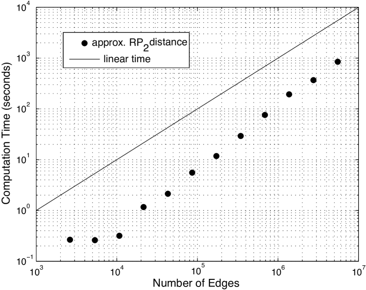
Figure 3: Computation time for $\widetilde{d}_{rp2}$ as a function of the number of edges $m={\cal O}(n)$.

This generates sparse random graphs with edge counts approximately proportional to the vertex counts.

In Fig. 3 we see that the computation time scales nearly linearly in the number of edges.

8 Fast Optimal Design of Networks Using the RP-1 Distance

Improving network robustness via targeted edge addition is a problem with considerable applications. The Kirchhoff index is often used as a measure of network robustness (see e.g., Wang et al. [53] and references therein). A lower Kirchhoff index is indicative of a more robust network, since lower effective resistances between pairs of vertices is indicative of short and/or redundant paths between vertices. The greedy approach, which consists in connecting the pair of vertices with the highest effective resistance, is known to be suboptimal (e.g., Ellens et al. [18]). Wang et al. [53] demonstrate however, that choosing the maximum effective resistance is often close to optimal, and can be accomplished in $O(n^{3})$ time rather than $O(n^{5})$ as required for an exhaustive search.

We make the following significant contribution to this question: we propose an algorithm with complexity ${\cal O}(n)$ to approximate the optimal edge addition. Specifically, this novel algorithm combines a low-rank approximation of the exact $\operatorname{d_{\operatorname{rp}1}}$ distance given by theorem 67 with a fast heuristic. We describe these two components in the next sections.

8.1 Low-rank Approximation of the RP-1 Distance

Theorem 37 provides an exact formula for computing the perturbation of the Kirchhoff index due to changes (addition, or removal) in a single edge. The optimal edge addition can thus be computed with a complexity $O(n^{3})$ time. Indeed, $O(n^{3})$ operations are needed to compute the spectral decomposition of $\bm{L}$; another $O(n)\times O(n^{2})$ operations are then required to exhaustively compute the exact $\operatorname{d_{\operatorname{rp}1}}(G,G+{\Delta w_{i_{0}j_{0}}})$ distance (in $O(n)$ operations using (37)), for every pair of vertices $i_{0}$ and $j_{0}$.

The $O(n^{3})$ complexity is a significant improvement over the $O(n^{5})$ algorithm described in Wang et al. [53]. However, $O(n^{3})$ is still prohibitively expensive for large networks, which motivates us to consider a low-rank approximation strategy to reduce the cost of solving the optimal edge modification problem.

Many graphs exhibit a concentration of the bulk of the eigenvalues of the graph Laplacian [14]. In this case, the bulk is well separated from the smallest eigenvalues, and because it is well confined, it can be replaced by a single “representative” eigenvalue. This idea leads to the following approximations, which prove to be very accurate in practice, for the summations in (37).

Theorem 10 (Low-rank approximation)

The sums in the numerator and denominator in (37) can be approximated using the following lower and upper bounds,

$$\begin{split}\frac{2}{\lambda^{2}_{n}}+\sum_{k=2}^{p}\left\{\mspace{-4.0mu}\frac{1}{\lambda^{2}_{k}}-\frac{1}{\lambda^{2}_{n}\mspace{-4.0mu}}\right\}&\mspace{-4.0mu}\left[\bm{\phi}_{k}(i)-\bm{\phi}_{k}(j)\right]^{2}\leq\sum_{k=2}^{n}\frac{1}{\lambda^{2}_{k}}\mspace{-4.0mu}\left[\bm{\phi}_{k}(i)-\bm{\phi}_{k}(j)\right]^{2}\\ &\leq\frac{2}{\lambda^{2}_{p}}+\sum_{k=2}^{p}\mspace{-4.0mu}\left\{\mspace{-4.0mu}\frac{1}{\lambda^{2}_{k}}-\frac{1}{\lambda^{2}_{p}}\right\}\mspace{-4.0mu}\left[\bm{\phi}_{k}(i)-\bm{\phi}_{k}(j)\right]^{2}\mspace{-4.0mu},\end{split}$$ (66)

and

$$\begin{split}\frac{2}{\lambda_{n}}+\sum_{k=2}^{p}\left\{\mspace{-4.0mu}\frac{1}{\lambda_{k}}-\frac{1}{\lambda_{n}}\mspace{-4.0mu}\right\}&\mspace{-4.0mu}\left[\bm{\phi}_{k}(i)-\bm{\phi}_{k}(j)\right]^{2}\leq\sum_{k=2}^{n}\frac{1}{\lambda_{k}}\mspace{-4.0mu}\left[\bm{\phi}_{k}(i)-\bm{\phi}_{k}(j)\right]^{2}\\ &\leq\frac{2}{\lambda_{p}}+\sum_{k=2}^{p}\mspace{-4.0mu}\left\{\mspace{-4.0mu}\frac{1}{\lambda_{k}}-\frac{1}{\lambda_{p}\mspace{-4.0mu}}\right\}\mspace{-4.0mu}\left[\bm{\phi}_{k}(i)-\bm{\phi}_{k}(j)\right]^{2}\mspace{-4.0mu}.\end{split}$$ (67)

Proof of Theorem 10

The proof relies on the orthonormality of the eigenvectors to bound the contribution of the bulk of the spectrum ($\lambda_{p},\ldots,\lambda_{n}$) from above and below. See details in B.8.

Using the above result, we can approximate (37) using a partial set of eigenpairs. Corollary 181 in B.9 provides the corresponding bounds. In the next section we evaluate numerically the quality of the low-rank approximations provided by theorem 67. Our experiments indicate that close-to-optimal results (as measured by the reduction in the Kirchhoff index) can be achieved with $p\ll n$ eigenpairs.

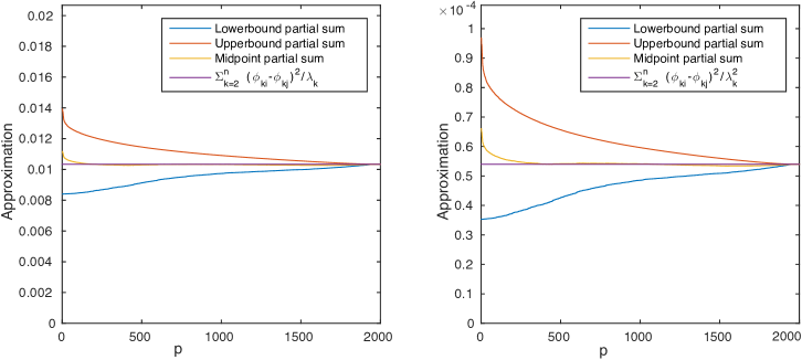
Two communities planted partition model

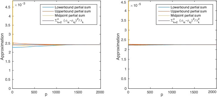
Small world (Watts and Strogatz) model

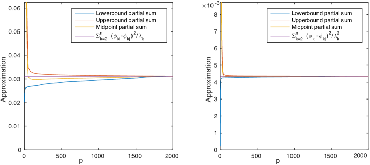
       $\sum_{k=2}^{n}\mspace{-4.0mu}\left[\bm{\phi}_{k}(i)-\bm{\phi}_{k}(j)\right]^{2}/\lambda_{k}$ $\sum_{k=2}^{n}\mspace{-4.0mu}\left[\bm{\phi}_{k}(i)-\bm{\phi}_{k}(j)\right]^{2}/\lambda_{k}^{2}$

Figure 4: The lower, upper, and average bounds given by theorem 67, as well as the exact sum for $\sum_{k=2}^{n}\mspace{-4.0mu}\left[\bm{\phi}_{k}(i)-\bm{\phi}_{k}(j)\right]^{2}/\lambda_{k}$ (left) and $\sum_{k=2}^{n}\mspace{-4.0mu}\left[\bm{\phi}_{k}(i)-\bm{\phi}_{k}(j)\right]^{2}/\lambda_{k}^{2}$ (right). All the quantities are displayed as a function of $p$, the number of eigenpairs used in the partial sums, (67) and (66). All graphs have $n=2,000$ vertices. See main text for details.

We generated several graphs from ensembles of random graphs, and computed the upper and lower bounds for both sums (66), and (67). To further improve the approximation, we noticed that the average of the lower and upper bounds in (66) and (67) produced a very accurate estimates of the corresponding sum. Indeed, the idea is that the bulk is approximated by the average of the largest and (one of) the smallest eigenvalue in the bulk. Fig. 4 displays the various approximations. The left column shows the approximation of $\sum_{k=2}^{n}\mspace{-4.0mu}\left[\bm{\phi}_{k}(i)-\bm{\phi}_{k}(j)\right]^{2}/\lambda_{k}$, while the left column displays the approximation of $\sum_{k=2}^{n}\mspace{-4.0mu}\left[\bm{\phi}_{k}(i)-\bm{\phi}_{k}(j)\right]^{2}/\lambda_{k}^{2}$.

Each row corresponds to a different graph. All graphs have $2,000$ vertices. The top row is a realization of an Erdős-Rényi random graph with edge probability equal to $0.1$. The middle row corresponds to a block stochastic model composed of two communities of equal sizes (also know as a planted partition model), where the within-community edge probability is $p_{\text{in}}=0.9$, and the between-community edge probability is $p_{\text{out}}=0.005$. Finally, the bottom row corresponds to a small world (Watts and Strogatz) model constructed by randomly re-wiring a regular ring lattice of constant degree 80, where each edge is rewired with a probability $\beta=0.01$. We conclude that for all three graphs, the average of the lower and upper bounds in (66) and (67) provided an accurate estimate of the numerator and the denominator of $\operatorname{d_{\operatorname{rp}1}}(G,G+{\Delta w_{i_{0}j_{0}}})$.

8.2 Fast greedy Optimization of the Kirchhoff Index

To avoid the exhaustive search of the optimal edge over all pairs of vertices, we designed the following fast greedy search method. The algorithm iteratively constructs a sequence of edges that converges toward a local optimum of (37). The initial edge is constructed by choosing randomly a vertex $i_{0}$. The algorithm then visits the other $n-1$ vertices, and select that vertex $j_{0}$ that maximizes the decrease in the Kirchhoff index, as measured by (37). The vertex $j_{0}$ is then kept fixed, and the algorithm visits the remaining $n-2$ vertices to replace $i_{0}$ by $i_{1}$ in order to further decrease (37) using the edge $[i_{1},j_{0}]$. The process is repeated until (37) can no longer be improved. This algorithm runs in ${\cal O}\left(n\right)$ time, a significant improvement over the $O(n^{2})$ exhaustive search.

8.3 Experimental Validation of the Optimization of the Kirchhoff Index

To validate the fast optimization of the Kirchhoff index, we designed a second set of experiments, using graphs generated from archetypal ensembles of random graphs. In this set of experiments, all graphs have 500 vertices. For all experiments we approximated the $\operatorname{d_{\operatorname{rp}1}}$ distance using the average of the lower and upper bounds (66) and (67) for the numerator and denominator of (37), respectively. This led to an estimate of the decrease of the Kirchhoff index, $\Delta\operatorname{{KI}}$, that was computed using $p$ eigenvectors. As $p$ increases and approaches $n$, we recover the exact expression given by (37). The gold standard, $\Delta\operatorname{{KI}}_{\text{optimal}}=\operatorname{d_{\operatorname{rp}1}}(G,G+{\Delta w_{\text{optimal}}})$, is the optimal decrease of the Kirchhoff index that would result from the optimal edge addition if we were to use an exhaustive search. Each plot in Fig. 5 displays the relative error, $\Delta\operatorname{{KI}}/\Delta\operatorname{{KI}}_{\text{optimal}}$ as a function of $p$. For each random graph model, the experiment was repeated 50 times.

The mean and the range (minimum to maximum, shown as an error-bar) of the relative reduction in the Kirchhoff index is plotted in Fig. 5. We note that this error compounds two approximations: the low-rank approximation in (67), and the greedy algorithm described in section 8.2.

We now describe the five graph models.

Unit Circle Latent Space Model. We sampled 500 points using a uniform distribution on the unit circle in $\mathbb{R}^{2}$,

$$\bm{x}_{i}=\begin{bmatrix}\cos(\theta_{i})\\ \sin(\theta_{i})\end{bmatrix},\quad\text{where}\;\theta_{i}\sim\text{U}[0,2\pi],\quad i=1,\ldots,500.$$

An unweighted graph $G=(V,E)$ was then generated by randomly connecting each pair of vertices $\{i,j\}$ with an edge $[i,j]$ according to a probability prescribed by a Gaussian kernel in the latent space,

$$P([i,j]\in E)=\frac{10}{\sqrt{\pi}}\exp\left(-100\|\bm{x}_{i}-\bm{x}_{j}\|^{2}\right),\quad\text{for}\;i\neq j.$$ (68)

Erdős-Rényi random graph. We constructed a random graph with edge probability equal to 0.05.

Two communities stochastic block model. We generated a stochastic block model formed by two communities of equal sizes, where the within-community edge probability was $p_{\text{in}}=0.1$, and the between-community edge probability was $p_{\text{out}}=0.01$.

Barabási-Albert preferential attachment model. The graph was constructed by sequentially adding two edges from each new vertex, attaching to other vertices with probability proportional to their current degrees.

Watts and Strogatz model. The small world model was designed by randomly re-wiring a regular ring lattice of constant degree 40 and a rewiring probability $\beta=0.1$.

We first notice in Fig. 5 that, for all graphs, the greedy search performed as well, or nearly as well, as the exhaustive search. With regard to the quality of the low-rank approximation, using only the Fiedler vector ($\bm{\phi}_{2}$), we were able to capture 95% of the optimal increase in the Kirchhoff index. The Erdős Rényi graph only required $\bm{\phi}_{2}$ to estimate the optimal $\Delta\operatorname{{KI}}_{\text{optimal}}$. As expected, the two-communities stochastic block model required two eigenvectors $\bm{\phi}_{2}$ and $\bm{\phi}_{3}$ to achieve near-optimal approximation. The latent space model required more eigenvectors to completely recover the optimal $\Delta\operatorname{{KI}}_{\text{optimal}}$. Nevertheless, a very good estimate was obtained with $\bm{\phi}_{2}$ only, which was able to capture the topological structure of the latent space formed by the ring. The stochastic nature of the graph construction necessitated more eigenvectors to fully

Erdős-Rényi random graph

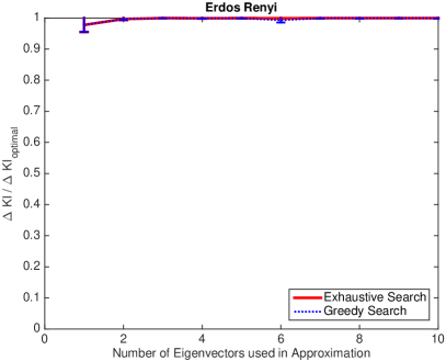
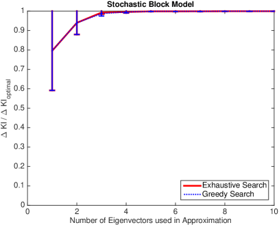
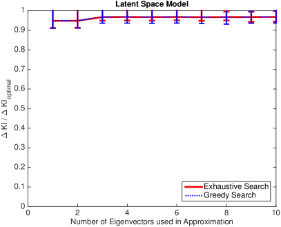
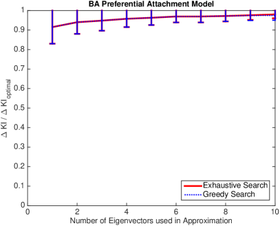
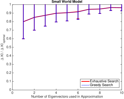
Figure 5: Relative reduction in the Kirchhoff index $\Delta\operatorname{{KI}}/\Delta\operatorname{{KI}}_{\text{optimal}}$ as a function of $p$, the number of eigenvectors used to approximate (37). We compare the exhaustive (solid red line) with the fast greedy search (dotted purple line). From left to right and top to bottom: Erdős-Rényi, stochastic block model, latent space model, Barabási-Albert preferential attachment, and Watts and Strogatz model. The mean relative reduction, as well as the range (minimum to maximum values, over 50 random realizations) are shown.

estimate the increase in the Kirchhoff index. A similar phenomenon happened with the Barabási-Albert preferential attachment model and the Watts and Strogatz model. In the latter case, $\bm{\phi}_{2}$ was only able to recover the ring lattice, which corresponds to the regular part of the graph. Additional eigenvectors were needed to capture the “disorder” created by the random rewiring. As mentioned earlier, the error is a function of the low-rank approximation in (67) and the greedy algorithm described in section 8.2, and therefore is not necessarily monotonically decreasing with $p$.

9 Analysis of Dynamic Networks with the RP-p Distances

We demonstrate in this section how the RP-1 and RP-2 distances can be used to detect anomalies caused by significant structural changes in dynamic networks. Our analysis is based on a series of experiments on synthetic and real networks. The results of the experiments clearly show that the resistance perturbation metric can detect the configurational changes in dynamic graphs that are triggered by appreciable modifications of the hidden variables controlling the graph dynamics.

The distances $\operatorname{d_{\operatorname{rp}1}}$ $\operatorname{d_{\operatorname{rp}2}}$, DeltaCon using $d_{\text{rootED}}$ (see (9) and (10)), and $d_{\text{CAD}}$ (see (18)) were computed for all the experiments. We used all the edges to compute $d_{\text{CAD}}$, to wit $F=E$ in (18).

9.1 Random Graphs Models

The first set of experiments rely on realizations of graphs sampled from ensembles of random graphs. The experiments were conducted on three different families of random graph models: a random graph with a latent space, a two-communities block stochastic model, and a Watts and Strogatz model. All models depend on a single scalar that characterizes the structure of the graph. We first detail the experimental procedure, and then describe each graph model.

Experimental procedure. All experiments were conducted in the following manner: a baseline graph $G^{(1)}$ was randomly selected using the baseline value for the parameter of the corresponding model. We then generated 50 random realizations of a second graph $G^{(2)}$, using the same value of the parameter.

The parameter that controls the graph was then increased, in 10 increments. For each increment, 50 random realizations of a second graph $G^{(2)}$ were constructed, and all the graph distances were computed. By modifying the parameter that has an important impact on the structure of the graphs, we evaluated quantitatively the relationship between the resistance perturbation distance and (potentially unobserved) changes in the latent parameter that controls the organization of the graph.

Our experiments show that the resistance perturbation distance is highly correlated with the evolution of the parameter that governs the structure of the graphs. In contrast, the DeltaCon distance is very sensitive to the normal fluctuations between the 50 random different realizations of the same exact graph structure. The DeltaCon distance also exhibits the largest variability between the different random realizations. The $d_{\text{CAD}}$ distance, which is biased by changes in the adjacency matrix can become too sensitive to changes in the graph topology (e.g., in the case of the stochastic block model).

Unit Circle Latent Space. A first graph $G^{(1)}$ was constructed by first sampling 2,000 points using a uniform distribution on the unit circle in $\mathbb{R}^{2}$,

$$\bm{x}^{(1)}_{i}=\begin{bmatrix}\cos(\theta^{(1)}_{i})\\ \sin(\theta^{(1)}_{i})\end{bmatrix}\mspace{-4.0mu},\;\text{with}\quad\theta^{(1)}_{i}\sim\text{U}[0,2\pi],\quad i=1,\ldots,2,000.$$

An unweighted graph $G^{(1)}=(V,E^{(1})$ was then generated by randomly connecting each pair of vertices $\{i,j\}$ with an edge $[i,j]$ according to a probability prescribed by a Gaussian kernel in the latent space,

$$P([i,j]\in E^{(1)})=\frac{20}{\sqrt{\pi}}\exp\left(-400\|\bm{x}_{i}-\bm{x}_{j}\|^{2}\right),\quad\text{for}\;i\neq j.$$ (69)

                     unit circle latent space model                                  two communities stochastic block model

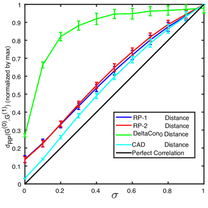
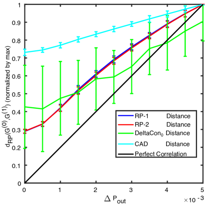
    small world (Watts and Strogatz) model

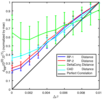
Figure 6: The graph distances $\operatorname{d_{\operatorname{rp}1}}(G^{(1)},G^{(2)})$, $\operatorname{d_{\operatorname{rp}2}}(G^{(1)},G^{(2)})$, DeltaCon (${d_{\text{rootED}}\left({G^{(1)}},{G^{(2)}}\right)}$), and $d_{\text{CAD}}(G^{(1)},G^{(2)})$, as a function of the latent parameter that controls the structural difference between $G^{(1)}$ and $G^{(2)}$. Error bars represent the standard deviation computed over 50 random realizations. Top: unit circle latent space model (left), and the two communities stochastic block model (right). Bottom: the small world (Watts and Strogatz) model. See text for details.

A second random graph $G^{(2)}=(V,E^{(2)})$ was generated according to the same principle, but with a second set of latent locations, $\{\bm{x}^{(2)}_{i}\}$ that was obtained by a perturbation of the initial set $\{\bm{x}^{(1)}_{i}\}$,

$$\bm{x}^{(2)}_{i}=\begin{bmatrix}\cos(\theta^{(2)}_{i})\\ \sin(\theta^{(2)}_{i})\end{bmatrix}\mspace{-4.0mu},\;\text{with}\quad\theta^{(2)}_{i}=\theta^{(1)}_{i}+\gamma_{i},\;\gamma_{i}\sim{\cal N}(0,\sigma^{2}),\;i=1,\ldots,2,000.$$

The random edges $E^{(2)}$ were connected using the same probability distribution given by (69). The magnitude of the random Gaussian shifts between the angles of the set $\{\bm{x}^{(1)}_{i}\}$ and those of the set $\{\bm{x}^{(2)}_{i}\}$ is controlled by the standard deviation $\sigma$. For increasing values of $\sigma\in[0,1]$ we constructed 50 random realizations of $G^{(2)}$, and we computed $\operatorname{d_{\operatorname{rp}1}}(G^{(1)},G^{(2)})$ and $\operatorname{d_{\operatorname{rp}2}}(G^{(1)},G^{(2)})$.

Figure 6 top-left displays all the graph distances as a function of $\sigma$. We first observe that $\operatorname{d_{\operatorname{rp}1}}(G^{(1)},G^{(2)})$ and $\operatorname{d_{\operatorname{rp}2}}(G^{(1)},G^{(2)})$ are very similar. This is crucial, since we designed a fast algorithm to approximate $\operatorname{d_{\operatorname{rp}2}}$. We also note that both RP distances are highly correlated with the magnitude of the perturbation, $\sigma$.

The increasing difference between $G^{(1)}\mspace{-4.0mu}$ and $G^{(2)}\mspace{-4.0mu}$, created by the increase in $\sigma$, intensifies the “disorganization” of $G^{(2)}$; the latent model is less and less regularly organized along the unit circle. The DeltaCon distance is able to detect this progression toward disorder, but quickly reaches its maximum value for unremarkable values of $\sigma$, making it useless for detecting anomalies. In contrast the $d_{\text{CAD}}$ distance performed extremely well.

Two Communities Stochastic Block Model. The $n=2,000$ nodes are divided into two communities of size $n/2$. Every pair of nodes $\{i,j\}$ forms an edge $[i,j]$ with probability $p_{\text{in}}$ if they belong to the same community, and with probability $p_{\text{out}}$ if they belong to different communities. We fixed $p_{\text{in}}=0.9$ for both graphs. We used $p^{(1)}_{\text{out}}=0.005$ for $G^{(1)}$, and we varied $p^{(2)}_{\text{out}}\in[0.005,0.01]$ for $G^{(2)}$. Figure 6 top-right displays the four graph distances as a function of $\Delta p_{\text{out}}=p^{(2)}_{\text{out}}-p^{(1)}_{\text{out}}$.

In comparison with the latent space model, we note that the changes in the adjacency matrix created by the intrinsic randomness of the model confuses the $d_{\text{CAD}}$ distance very quickly. Indeed, the $d_{\text{CAD}}$ distance immediately reaches 0.73 in the baseline condition when $G^{(1)}$ and $G^{(2)}$ have the same structure, to wit when they are both realizations of the same random model (same $p_{\text{in}}$ and same $p_{\text{out}}$). DeltaCon is equally confused: the standard deviation is very large, making it difficult to assess the confidence one should attach to a single measurement of the distance.

Conversely, $\operatorname{d_{\operatorname{rp}1}}(G^{(1)},G^{(2)})$ are highly correlated with the increase in $p_{\text{out}}$, making the distances suitable to detect changes in community networks. Furthermore, the standard deviations for both RP-distances remain very small.

Small World Model. We generated random realizations of a small world (Watts and Strogatz) model constructed by randomly re-wiring a regular ring lattice of constant degree 40 using a random rewiring with probability $\beta_{2}$ that varied from $\beta_{2}=\beta_{1}=0.01$ for $G^{(1)}$, to $\beta_{2}=0.02$. We generated 50 random realizations for each value of $\beta_{2}$. Figure 6-bottom displays the four graph distances as a function of $\Delta\beta=\beta_{2}-\beta_{1}$.

In this model, the initial ring lattice moves toward a state of disorder when $\beta_{2}$ increases. In a manner comparable to the latent space model, the increase in disorganization is detected by the DeltaCon distance, which is correlated with $\Delta\beta$ over the entire range. Both RP-distances as well as the $d_{\text{CAD}}$ distance are more tightly correlated with the increase of $\Delta\beta$, and are therefore more suitable to infer the dynamic underlying changes in the graph.

9.2 Real Dynamic Network

The second set of experiments involved two real-world dynamic networks, where we can qualitatively compare the resistance perturbation distance to known events that would likely influence the behavior of actors in the dynamic networks. These results suggest that the resistance perturbation metric can identify changes in real dynamic graphs, and could be used to infer changes in the hidden variables that govern the evolution of such dynamic graphs. Enron email network. The Enron email corpus [27] is composed of the email messages between approximately 150 high-level executives (the Enron “core”); these were included in the analysis because these individuals were most closely involved in the scandal. Emails were aggregated on a weekly basis to generate a dynamic series of communication graphs, and compared to a timeline of events. Undirected edges were assigned between pairs of vertices, with a weight equal to the number of emails exchanged between the two people during a given week. In order to focus on personal communications, emails with greater than three recipients were excluded from the analysis. The size of the remaining dynamic graph is: number of vertices = 151; count of emails = 31534; count of weighted

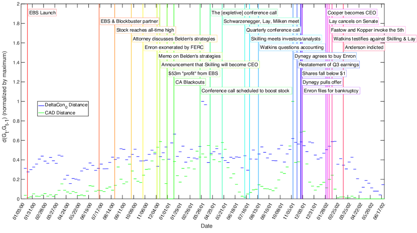
Figure 7: $\operatorname{d_{\operatorname{rp}1}}$ and $\operatorname{d_{\operatorname{rp}2}}$ (top) and DeltaCon ($d_{\text{rootED}}$) and $d_{\text{CAD}}$ (bottom) between consecutive weekly email graphs from the Enron corpus. Notable events in the timeline of the company’s collapse are also plotted for reference [39].

edges after weekly aggregation = 7794. The time period analyzed spans the period leading up to the Enron scandal and subsequent collapse of the company.

The resistance perturbation metrics, $d_{rp1}$ and $d_{rp2}$, between consecutive weekly email graphs are plotted in Fig. 7-top; $d_{rp1}$ and $d_{rp2}$ have very similar dynamics. Furthermore, we note that large changes detected by $d_{rp2}$ during the summer and fall of 2001 are predictive of the events that lead to the ultimate collapse of the company.

An independent analysis of the same dataset [40, 41] confirms that changes in the mean degree, which are highly correlated to changes in the volume, is a very poor predictor of the changes detected by the RP-distance.

DeltaCon exhibits a lot of volatility, changing at times when there are no significant events in the company, while remaining constant around the time associated with notable events. Changes in the $d_{\text{CAD}}$ distance appear to be tightly coupled with the events described by the vertical bars.

MIT reality mining dataset. The MIT reality mining dataset [17] provides collocation information between a group of students and faculty at MIT during the course of an academic year. A dynamic undirected graph was built from weekly-aggregated Bluetooth proximity data. The weights of the edges in this dynamic graph are proportional to the amount of time each pair of cellphones registered one-another’s presence in close physical proximity.

The $d_{rp1}$ and $d_{rp2}$ metrics between consecutive weekly proximity graphs are plotted in Fig. 8-top. We again note that $d_{rp1}$ and $d_{rp2}$ appear to be within a constant factor of one another. Both metrics can predict events during the course of the academic year. A substantial change between the first and second week of classes at the beginning of the fall semester is likely representative of students sorting out their class schedules and friend groups. The week after finals (the beginning of winter break) and the beginning of the independent activities period are reflected by significant changes in the network, as measured by the $d_{rp1}$ and $d_{rp2}$ metrics. The network also changes at the beginning and end of spring break, as students depart from and return to their campus routine. For comparison, we present a similar analysis using the DeltaCon and $d_{\text{CAD}}$ distances in Fig. 8-bottom. Both distances appear to detect changes during the academic calendar (e.g., sponsor week, finals week, etc.) DeltaCon appears to be more stable then $d_{\text{CAD}}$.

Because of the nature of the data, the RP distances can be used to confirm behavioral changes associated with the geolocation of the different actors (nodes) of the network. Unlike the Enron dataset, the RP distance has no predictive value in this case, but can be used to grade the significance of the changes in behavior: finals are more important than spring break, which is more important than exam week. Finals week appears to be more important than the beginning of the semester.

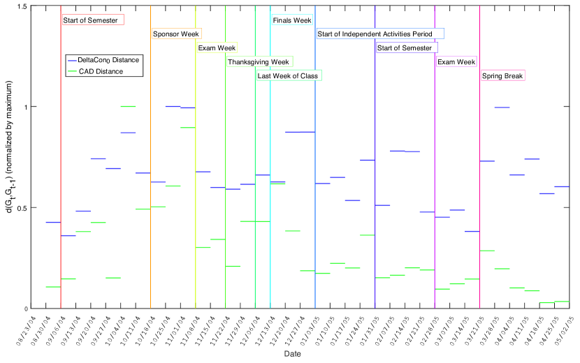
Figure 8: $\operatorname{d_{\operatorname{rp}1}}$ and $\operatorname{d_{\operatorname{rp}2}}$ (top) and DeltaCon ($d_{\text{rootED}}$) and $d_{\text{CAD}}$ (bottom) between consecutive weekly Bluetooth proximity graphs from the MIT Reality Mining dataset. Important events in the academic calendar are also plotted [39].

10 Discussion

We revisit the goal of the paper and confirm that the resistance perturbation distance RP-p satisfies the axiom and principles laid out in section 3.1.

10.1 Adherence to Axioms and Principles

Axiom 1. We have indeed proved in theorem 1 that all the RP-p distances were proper distances, and therefore this family of distances satisfies Axiom 1.

Principle 1: Edge Importance. Remark 3 in section 5.3 proves that
$\operatorname{d_{\operatorname{rp}1}}(G,G+{\Delta w_{i_{0}j_{0}}})\rightarrow\infty$ if and only if removing the edge $[i_{0},j_{0}]$ disconnects the graph, thereby proving Principle 1.

Principle 2: Weight Awareness As explained in Remark 3 in section 5.3, as $w_{i_{0}j_{0}}\rightarrow\infty$, then $A^{-1}_{i_{0}j_{0}}\approx R_{i_{0}j_{0}}$, and $1-w_{i_{0}j_{0}}R_{i_{0}j_{0}}\approx 0$, leading the distance $\operatorname{d_{\operatorname{rp}1}}(G,G+{\Delta w_{i_{0}j_{0}}})$ to go to infinity when the edge is removed, to wit when ${\Delta w_{i_{0}j_{0}}}=-w_{i_{0}j_{0}}$. The second principle of “weight awareness” is therefore clearly satisfied: as the weight of the removed edge grows, the distance grows to infinity.

Principle 3: Edge-“Submodularity”. While we do not have a formal proof of this principle, we can use the comparison of the complete graph (theorem 3) with the star graph (theorem 4) to illustrate the scaling of the distance $\operatorname{d_{\operatorname{rp}1}}$. The complete graph has $O(n^{2})$ edges, and $\operatorname{d_{\operatorname{rp}1}}(K_{n},K_{n}+{\Delta w_{i_{0}j_{0}}})=O(1/n)$. The star graph has $O(n)$ edges, and $\operatorname{d_{\operatorname{rp}1}}(S_{n},S_{n}+{\Delta w_{i_{0}j_{0}}})=O(n)$. In this example, changes made to a sparse graph are more important than equally sized changes made to a denser graph with the same number of vertices.

Instead of comparing a single-edge perturbation of graphs that have different topologies, and thus different densities, we can evaluate the perturbation of graphs that have the same topology, but different densities.

We illustrate this concept with a stochastic block model composed of size $n=1,000$. The nodes are divided into two communities of size $n/2$. Every pair of nodes $\{i,j\}$ forms an edge $[i,j]$ with probability $p$ if they belong to the same community, and with probability $q$ if they belong to different communities. We fixed $p=\log^{2}(n)/n$, and we increase $q$ from $\log(n)/n^{2}$ to $7p/n$.

For each value of $q$ we generate 200 realizations of the model. For each realization $G$, we perturb a single edge, $e$. The edge is chosen at random within one of the two communities (within community perturbations), or chosen to be one of the cross-community edges (cross community perturbation). We then compute the distances between $G$ and $G\backslash\{e\}$ – $G$ with the edge $e$ removed.

Figure 9 displays the distances ${d_{\operatorname{DC}_{0}}\left({G},{G\backslash\{e\}}\right)}$ and $\operatorname{d_{\operatorname{rp}1}}\left(G,G\backslash\{e\}\right)$ as a function of the probability $q$ of connecting the two balanced communities. Each of the distance time-series is normalized by its maximum value, and the error-bars display the standard deviations computed over 200 realizations. The blue line corresponds to the theoretical analysis of $\operatorname{d_{\operatorname{rp}1}}\left(G,G\backslash\{e\}\right)$ performed in [54], which corresponds to a power-law decay (note the logarithmic scale).

We note that $d_{\operatorname{DC}_{0}}$ is sensitive to the type of edges that is being removed: the distance is larger for cross-community edges (see Fig. 9 magenta). However, $d_{\operatorname{DC}_{0}}$ is independent of the increasing density of the graph.

Similar to $d_{\operatorname{DC}_{0}}$, $\operatorname{d_{\operatorname{rp}1}}$ can easily detect whether the deleted edge $e$ was removed from within a community, or was a cross-community edge. In contrast to $d_{\operatorname{DC}_{0}}$, the distance $\operatorname{d_{\operatorname{rp}1}}$ is very sensitive to the density of edges in the graph. In agreement to principle 3, $\operatorname{d_{\operatorname{rp}1}}$ decreases as a function of the graph density.

Principle 4: Focus Awareness. The fourth principle, “focus awareness”, states that random changes in graphs are less important than targeted changes of the same extent. While the notion of targeted versus random changes would need to be defined more precisely, we argue that remark 4 in section 5.3 addresses this principle. Indeed, in the example of a network formed by densely connected communities, which are weakly connected to one another, $\operatorname{d_{\operatorname{rp}1}}(G,G+{\Delta w_{i_{0}j_{0}}})$ will be maximal if $i_{0}$ and $j_{0}$ are in different communities, for the same ${\Delta w_{i_{0}j_{0}}}$. Because there are much fewer edges bridging the communities, modifying the edge $[i_{0},j_{0}]$,

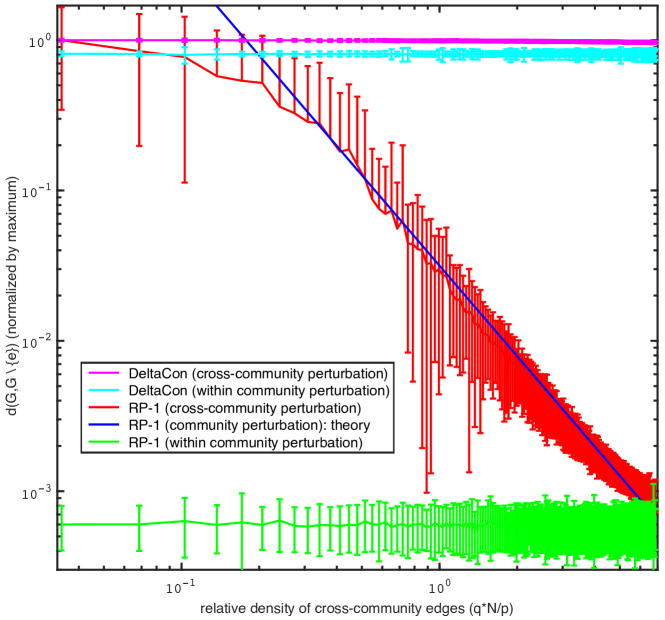
Figure 9: The distances ${d_{\operatorname{DC}_{0}}\left({G},{G\backslash\{e\}}\right)}$ and $\operatorname{d_{\operatorname{rp}1}}\left(G,G\backslash\{e\}\right)$ as a function of the probability $q$ of connecting two balanced communities of size $n/2=500$. Each time-series is normalized by its maximum value, and the error-bars display the standard deviation computed over 200 realizations. For each distance, the perturbed edge $e$ can either belong to one of the two communities (within community perturbation), or be one of the cross-community edges (cross community perturbation).

where $i_{0}$ and $j_{0}$ are in different communities, is indeed a targeted change.

We conclude that the resistance perturbation distance satisfies the axiom and principles (see section 3.1) that a graph distance should obey. These principles were inspired by the pioneering work of Koutra et al. [29], where the authors compared the DeltaCon algorithm to vertex edge overlap [36], the graph edit distance [10], the signature similarity [36], and three variations of the $\lambda$-similarity [10, 38, 55]. The authors in [29] show that DeltaCon is the only algorithm that adheres to their set of axioms and principles. In fact, our asymptotic analyses of the DeltaCon₀ similarity for the complete and star graphs (A) demonstrates that this distance fails to meet Principle 3.

10.2 Future Work

The introduction of the resistance perturbation distance prompts several important research questions. A current limitation of the RP distance is its inability to measure distances between disconnected graphs in a meaningful way, which stems from the fact that the effective resistance between vertices in disconnected components of a graph is infinite. Thus, it may prove valuable to consider extensions of the resistance perturbation distance that accommodate disconnected graphs. One option may be to define a distance based on some comparison of the conductance matrices.

A volume-normalized version of the distance may also be of interest. In some applications, the user might be more interested in the overall structure of the graph, and less interested in the magnitude of the weights along the edges. For example, if all edge weights are doubled between one graph and another, this could be viewed as insignificant in some circumstances. The precise implications of such a normalization are a worthy direction for future research.

Many applications of the RP distance should be explored.

In the context of dynamic graphs (see section 9), the $\operatorname{d_{\operatorname{rp}(p)}}$ metric can be used to study the dynamic evolution of a graph sequence $\{G^{(n)}\}$, where $n$ denotes the time index of the corresponding element $G^{(n)}$ in the graph process. There has been some recent interest in the detection of anomalies in dynamic graphs [2, 31, 42]. Formally, one can construct a statistic $Z_{n}$, based on the distance $D_{n}=\operatorname{d_{\operatorname{rp}(p)}}(G^{(n)}_{n},G_{n+1})$ between $G^{(n)}$ and $G^{(n+1)}$, in order to test the hypothesis $H_{0}$ that the graphs $G^{(n)}$ and $G^{(n+1)}$ are structurally the same against the alternate hypothesis that $G^{(n)}$ and $G^{(n+1)}$ are structurally different. In this context, we accept $H_{0}$ if $Z_{n}<z_{\varepsilon}$ and accept $H_{1}$ otherwise. The threshold $z_{\varepsilon}$ for the rejection region satisfies

$$\operatorname{Prob}_{H_{0}}\left(Z_{n}\geq z_{\varepsilon}\right)\leq\varepsilon\quad\text{as}\quad n\rightarrow\infty,$$ (70)

and

$$\operatorname{Prob}_{H_{1}}\left(Z_{n}\geq z_{\varepsilon}\right)\rightarrow 1\quad\text{as}\quad n\rightarrow\infty.$$ (71)

The test has therefore asymptotic level $\varepsilon$ and asymptotic power 1. Our recent work [54] develops the construction of the statistic $Z_{n}$ in the context of a dynamic community network.

Our results in section 9 on random graph models, clearly show that one can quantify the normal random fluctuations of the metric $d_{rp(p)}$ using ensemble of random graphs, which defines a notion of normal baseline “background” noise to be expected when a graph does not experience significant configurational changes. Furthermore, both $\operatorname{d_{\operatorname{rp}1}}$ and $\operatorname{d_{\operatorname{rp}2}}$ can detect significant structural changes, such as changes in topology, connectivity, or “disorder”. Formally, one can numerically estimate a $1-\varepsilon$ point wise confidence interval for the test statistic with a bootstrapping technique; the details of such a construction extend beyond the scope of the present report and are the subject of ongoing investigation [54].

While the metric $d_{rp(p)}$ can provide insightful information about changes at many different scales in the graph structure, it does not provide any localization about the anomalies. One could study the problem of attribution of the anomaly. A multiscale approach, where the metric $d_{rp(p)}$ is computed between corresponding subgraphs of $G^{(2)}$ and $G^{(2)}$, could provide insight into the localization of the metric changes. Alternatively, one could try to localize the anomalous edges using the approach proposed in [50], and described in section 3.2.

Spielman and Srivastava [48] introduced a method for generating sparse spectrally similar graphs by sampling edges of the original graph according to the effective resistance between endpoints of the edges. This strategy suggests a meaningful connection between effective resistances and spectral similarity. Indeed, Batson et al. [6] observed that spectrally similar graphs exhibit similar effective resistances between all pairs of vertices. Improving our understanding of potential connections between the spectral similarity and resistance perturbation distance is an avenue of significant interest for future work.

In this work, we have presented and implemented a fast algorithm to compute $d_{rp2}$. This effort leads to several questions. First, we observed that the computation time for the fast $d_{rp2}$ approximation algorithm is dominated by the $\widetilde{{\cal O}}(\log n)$ Laplacian linear solver (each of size $n$). Our current implementation utilizes the combinatorial multigrid solver of Koutis et al. [28]. Although we observe linear scaling of the algorithm on several scalable example problems, the constant hidden in the $\widetilde{{\cal O}}$ is unfortunately significant.

One could explore competing algorithms for the Laplacian solver. Lean Algebraic Multigrid (LAMG) [32, 33] is a competing method for solving graph Laplacian linear systems in linear time that may reduce the cost of approximating the $d_{rp2}$ metric. Given the diversity of structural features in graphs, an adaptive approach may be necessary to handle different types of graphs efficiently.

Modern high-performance computing architectures demand the development of highly parallelizable algorithms. The structure of the $d_{rp2}$ approximation algorithm lends itself to natural parallelism. The most direct opportunity for parallelism involves splitting the ${\cal O}(\log n)$ independent calls to the Laplacian solver onto independent processors/cores. Additionally, depending on the choice of the Laplacian solver algorithm, each call to the solver could potentially be parallelized. A detailed investigation of such algorithmic improvements is an important avenue for future work.

References

11 Notation

Symbol	Definition	(equation)
$G$	graph with vertex set $V$, edge set $E$, and edge weights $\bm{w}$	(1)
$[i,j]$	edge between nodes $i$ and $j$	(1)
$\bm{A}$	$n\times n$ adjacency matrix
	$A_{ij}=w_{ij}$ if $i$ and $j$ are connected, $0$ otherwise	(1)
$\bm{D}$	$n\times n$ diagonal matrix of vertex degrees, $D_{ii}=\sum_{j=1}^{n}A_{ij}$	(2)
$\bm{L}$	$n\times n$ combinatorial Laplacian matrix	(2)
$\bm{\phi}_{k},\lambda_{k}$	eigenvector and eigenvalue of $\bm{L}$, with $0=\lambda_{1}\leq\ldots\leq\lambda_{n}$	(3)
$\bm{L}^{\dagger}$	pseudoinverse of $\bm{L}$	(4)
$\bm{B}$	$m\times n$ edge incidence matrix	(7)
$\bm{{d\mspace{-1.0mu}A}}$	$m\times m$ diagonal edge weight matrix	(7)
$d_{\text{rootED}}$	root Euclidean distance	(10)
${\bm{S}}^{(i)}$	$n\times n$ fast belief propagation matrix	(11)
$\bm{e}_{i}$	$i$-th canonical basis vector $\bm{e}_{i}\in\mathbb{R}^{n}$
$\bm{R}$	$n\times n$ matrix of effective resistances	(22)
$\operatorname{{KI}}(G)$	Kirchhoff index of $G$	(24)
$\kappa_{ij}$	commute time between vertices $i$ and $j$	(25)
$\left\lVert\cdot\right\rVert_{p}$	element-wise p-norm	(28)
$d_{\operatorname{rp}(p)}$	resistance perturbation distance	(28)
$\widetilde{\bm{Z}}$	${\cal O}(\log n)\times n$ embedding matrix	(58)
$\bm{Q}$	${\cal O}(\log n)\times m$ random projection matrix	Algorithm 1
$p$	number of eigenvectors used
	in the low-rank approximation of $\operatorname{d_{\operatorname{rp}1}}$	(67)

Appendix A DeltaCon₀ Analysis

A.1 Introduction

In this section we compute analytically the DeltaCon₀ similarity for small perturbations of the complete and the star graphs. We restrict our attention to simple perturbations, where $G^{(2)}$ is generated from $G$ by a change in edge weight of size ${\Delta w_{i_{0}j_{0}}}$ between vertices $i_{0}$ and $j_{0}$.

Our main tool is the Sherman–Morrison–Woodburry theorem [23] that provides a closed form expression for the inverse of a low-rank perturbation of a non-singular matrix. For completeness, we recall the Sherman–Morrison–Woodburry formula.

If $\bm{X}$ is an $n\times n$ non singular matrix, and $\bm{U}$ and $\bm{V}$ are two $n\times k$ matrices, then $\bm{T}=\bm{I}+\bm{V}^{T}\bm{X}^{-1}\bm{U}$ is non singular if and only if

$$\bm{Y}=\bm{X}+\bm{U}\bm{V}^{T}$$ (72)

is non singular. Furthermore, when $\bm{Y}^{-1}$ exists, we have

$$\left[\bm{X}+\bm{U}\bm{V}^{T}\right]^{-1}=\bm{X}^{-1}-\bm{X}^{-1}\bm{U}\left[\bm{I}+\bm{V}^{T}\bm{X}^{-1}\bm{U}\right]^{-1}\bm{V}^{T}\bm{X}^{-1}.$$ (73)

In the following, we use this theorem with $k=1$ or $k=2$. When $k=1$, we have the Sherman–Morrison formula,

$$\left[\bm{X}+\bm{u}\bm{v}^{T}\right]^{-1}=\bm{X}^{-1}-\frac{1}{1+\bm{v}^{T}\bm{X}^{-1}\bm{u}}\bm{X}^{-1}\bm{u}\bm{v}^{T}\bm{X}^{-1}.$$ (74)

For the purpose of writing concise equations, we extend the big $\cal O$ notation for matrices. If $\widetilde{\bm{A}}(n)$ and $\bm{A}(n)$ are two sequences of matrices that depend on $n$, then the notation

$$\widetilde{\bm{A}}(n)=\bm{A}(n)+{\cal O}\left(1/n^{q}\right),$$ (75)

means that

$$\forall i,j,\quad\widetilde{a}_{ij}(n)=a_{ij}(n)+{\cal O}\left(1/n^{q}\right).$$ (76)

In other words, there exists a sequence of matrices $\bm{B}(n)=\left[b_{ij}^{(n)}\right]$ such that,

$$\exists\;c_{2}>c_{1}\geq 0,\quad\widetilde{\bm{A}}(n)=\bm{A}(n)+\bm{B}(n),\quad\text{and}\quad\forall n,\quad c_{1}\leq n^{q}b_{ij}(n)\leq c_{2}.$$ (77)

A.2 Complete Graph

In the case of the complete graph $G$ on $n$ vertices we have,

$$\bm{A}=\bm{J}-\bm{I},\quad\bm{D}=(n-1)\bm{I},\quad\text{and}\quad\varepsilon=\frac{1}{n}.$$ (78)

Then, the fast belief propagation matrix (11) is given by

$$\bm{S}=\left[\bm{I}+\frac{n-1}{n^{2}}\bm{I}-\frac{1}{n}\bm{J}+\frac{1}{n}\bm{I}\right]^{-1}=\left[\frac{n^{2}+2n-1}{n^{2}}\bm{I}-\frac{1}{n}\bm{1}\bm{1}^{T}\right]^{-1}$$ (79)

The Sherman–Morrison–Woodbury formula (73) yields

$$\bm{S}=\frac{n^{2}}{n^{2}+2n-1}\left\{\bm{I}-\frac{n}{2n-1}\bm{J}\right\}.$$ (80)

We now consider the perturbed graph $G^{(2)}$. Without loss of generality, we can assume that the edge $[1,2]$ was modified, and thus $G^{(2)}$ is obtained by the change $w_{12}\rightarrow w_{12}+{\Delta w_{12}}$. The perturbed adjacency matrix $\bm{A}^{(2)}$ is given by

$$\bm{A}^{(2)}\mspace{-6.0mu}=\begin{bmatrix}1&\mspace{-12.0mu}1+{\Delta w_{12}}&1&\cdots\\ 1+{\Delta w_{12}}&1&1&\cdots\\ 1&&\mspace{-12.0mu}\ddots&\\ \vdots\end{bmatrix},$$ (81)

and degree matrix $\bm{D}^{(2)}$ is given by

$$\bm{D}^{(2)}\mspace{-6.0mu}=\begin{bmatrix}n-1+{\Delta w_{12}}&&&&0\\ &\mspace{-50.0mu}n-1+{\Delta w_{12}}&&&\\ &&\mspace{-70.0mu}n-1&&\\ &&&\mspace{-50.0mu}\ddots&\\ 0&&&&\mspace{-20.0mu}n-1\end{bmatrix}.$$ (82)

The inverse of the fast belief propagation matrix of $G^{(2)}$ is given by

$$\left[\bm{S}^{(2)}\right]^{-1}=\bm{I}+\varepsilon_{2}^{2}\bm{D}^{(2)}-\varepsilon_{2}\bm{A}^{(2)},\quad\text{with}\quad\varepsilon_{2}=\frac{1}{n+{\Delta w_{12}}},$$ (83)

which simplifies to

$$\begin{split}\left[\bm{S}^{(2)}\right]^{-1}\mspace{-20.0mu}&=\frac{n^{2}+2n-(3{\Delta w_{12}}+1)}{n^{2}}\bm{I}-\frac{1}{n}\left(1-\frac{{\Delta w_{12}}}{n}+\frac{{\Delta w_{12}}^{2}}{n^{2}}\right)\bm{J}\\ -&\frac{{\Delta w_{12}}}{n}\left(1-\frac{{\Delta w_{12}}}{n}\right)\left(\bm{e}_{1}\bm{e}_{2}^{T}+\bm{e}_{2}\bm{e}_{1}^{T}\right)+\frac{{\Delta w_{12}}}{n^{2}}\left(\bm{e}_{1}\bm{e}_{1}^{T}+\bm{e}_{2}\bm{e}_{2}^{T}\right)+{\cal O}\left(1/n^{3}\right).\end{split}$$ (84)

We break $\left[\bm{S}^{(2)}\right]^{-1}$ into two parts. First, we apply the Sherman-Morrison formula (74) to get the inverse of a rank-one perturbation of a diagonal matrix,

$$\begin{split}&\left[\frac{n^{2}+2n-(3{\Delta w_{12}}+1)}{n^{2}}\bm{I}-\frac{1}{n}\left(1-\frac{{\Delta w_{12}}}{n}+\frac{{\Delta w_{12}}}{n^{2}}\right)\bm{1}\bm{1}^{T}\right]^{-1}\\ &=\frac{n^{2}}{n^{2}+2n-(3{\Delta w_{12}}+1)}\bm{I}+\frac{1}{2+{\Delta w_{12}}}\left(1-\frac{3+{\Delta w_{12}}}{n(2+{\Delta w_{12}})}\right)\bm{J}+{\cal O}\left(1/n^{2}\right).\end{split}$$ (85)

Then we add the rank-two perturbation, $-\frac{{\Delta w_{12}}}{n}\left(1-\frac{{\Delta w_{12}}}{n}\right)\left(\bm{e}_{1}\bm{e}_{2}^{T}+\bm{e}_{2}\bm{e}_{1}^{T}\right)$, and apply the Sherman–Morrison–Woodbury formula (73) to arrive at

$$\begin{split}\bm{S}^{(2)}&=\frac{n^{2}}{n^{2}+2n-(3{\Delta w_{12}}+1)}\left(\bm{I}+\frac{1}{2+{\Delta w_{12}}}\left(1+\frac{1+{\Delta w_{12}}}{n(2+{\Delta w_{12}})}\right)\bm{J}\right)\\ &+\frac{{\Delta w_{12}}}{n(2+{\Delta w_{12}})^{2}}\left\lgroup 2\bm{J}+(2+{\Delta w_{12}})\left(\bm{1}(\bm{e}_{1}+\bm{e}_{2})^{T}+(\bm{e}_{1}+\bm{e}_{2})\bm{1}^{T}\right)\right.\\ &\mspace{150.0mu}\left.+(2+{\Delta w_{12}})^{2}\left(\bm{e}_{1}\bm{e}_{2}^{T}+\bm{e}_{2}\bm{e}_{1}^{T}\right)\right\rgroup+{\cal O}\left(1/n^{2}\right).\end{split}$$ (86)

Which simplifies to

$$\begin{split}\bm{S}^{(2)}\mspace{-4.0mu}&=\frac{n^{2}}{n^{2}+2n-(3{\Delta w_{12}}+1)}\bm{I}+\frac{1}{2+{\Delta w_{12}}}\mspace{-4.0mu}\left[1+\frac{{\Delta w_{12}}-3}{n(2+{\Delta w_{12}})}\right]\mspace{-4.0mu}\bm{J}\\ &+\frac{{\Delta w_{12}}}{n}\mspace{-4.0mu}\left[\bm{e}_{1}\bm{e}_{2}^{T}+\bm{e}_{2}\bm{e}_{1}^{T}\right]+\frac{{\Delta w_{12}}}{n(2+{\Delta w_{12}})}\mspace{-4.0mu}\left(\bm{1}[\bm{e}_{1}+\bm{e}_{2}]^{T}+[\bm{e}_{1}+\bm{e}_{2}]\bm{1}^{T}\right)\mspace{-4.0mu}\\ &+{\cal O}\left(1/n^{2}\right).\end{split}$$ (87)

From (80) we derive the following first order approximation of $\bm{S}$

$$\bm{S}=\left(1-\frac{2}{n}\right)\bm{I}+\left(1-\frac{3}{2n}\right)\frac{1}{2}\bm{J}+{\cal O}\left(1/n^{2}\right)$$ (88)

We now proceed to compute the DeltaCon₀ similarity between $G$ and $G^{(2)}$. We need to estimate the size of the terms $\sqrt{S_{ij}}-\sqrt{S^{(2)}_{ij}}$. Because we expect a linear growth of the distance, we only need an approximation up to order 1.

We start with the off-diagonal entries. If $i\neq j$, we have

$$S_{ij}=\frac{1}{2}+{\cal O}\left(1/n\right),\quad\text{and}\quad S^{(2)}_{ij}=\frac{1}{2+{\Delta w_{12}}}+{\cal O}\left(1/n\right),$$ (89)

from which we get

$$\sqrt{S_{ij}}-\sqrt{S^{(2)}_{ij}}=\frac{1}{\sqrt{2}}-\frac{1}{\sqrt{2+{\Delta w_{12}}}}+{\cal O}\left(1/n\right).$$ (90)

And therefore,

$$\left(\sqrt{S_{ij}}-\sqrt{S^{(2)}_{ij}}\right)^{2}=\left(\frac{1}{\sqrt{2}}-\frac{1}{\sqrt{2+{\Delta w_{12}}}}\right)^{2}+{\cal O}\left(1/n\right).$$ (91)

Thus

$$\sum_{i,j=1;i\neq j}^{n}\left(\sqrt{S_{ij}}-\sqrt{S^{(2)}_{ij}}\right)^{2}=n(n-1)\left(\frac{1}{\sqrt{2}}-\frac{1}{\sqrt{2+{\Delta w_{12}}}}\right)^{2}+{\cal O}\left(n\right)$$ (92)

From which we conclude that

$$\sum_{i,j=1;i\neq j}^{n}\left(\sqrt{S_{ij}}-\sqrt{S^{(2)}_{ij}}\right)^{2}=\left(\frac{1}{\sqrt{2}}-\frac{1}{\sqrt{2+{\Delta w_{12}}}}\right)^{2}n^{2}+{\cal O}\left(n\right).$$ (93)

A similar calculation shows that the terms on the diagonal only contribute to a linear term,

$$\sum_{i=1}^{n}\left(\sqrt{S_{ii}}-\sqrt{S^{(2)}_{ii}}\right)^{2}={\cal O}\left(n\right),$$ (94)

since there are only $n$ such terms and they have the same order as the off-diagonal terms. Combining all the terms, and keeping only the highest order, we conclude that

$${d_{\text{rootED}}\left({G},{G^{(2)}}\right)}=\left|\frac{1}{\sqrt{2}}-\frac{1}{\sqrt{2+{\Delta w_{12}}}}\right\rvert n+{\cal O}\left(1\right).$$ (95)

Figure 2-left confirms experimentally the linear growth of ${d_{\text{rootED}}\left({G},{G^{(2)}}\right)}$, which implies the decay of the DeltaCon₀ similarity, and contradicts Principle 3 from Koutra et al. [29], which asserts that “A specific change is more important in a graph with few edges than in a much denser, but equally sized graph.” Indeed, one would expect that the similarity between $G$ and $G+{\Delta w_{12}}$ should increase with $n$, since the relative importance of the edge perturbation ${\Delta w_{12}}$ becomes negligible for large $n$.

A.3 Star Graph

We proceed with the analysis of ${d_{\text{rootED}}\left({G},{G^{(2)}}\right)}$ in the case of the star graph. The indices of the leaf nodes are $2,\ldots,n$, and the index of the hub is $1$. We follow the same sequence of steps as in the complete graph. First, we compute the exact expression of the fast belief propagation matrix (11), $\bm{S}$, using the Sherman–Morrison–Woodbury formula (73). We then perturb a single edge, and we compute the fast belief propagation matrix of the perturbed graph, $\bm{S}^{(2)}$, using again the Sherman–Morrison–Woodbury formula. Our analysis will be performed with precision $1/n^{2}$, since we expect that ${d_{\text{rootED}}\left({G},{G^{(2)}}\right)}$ decays as a function of $n$.

For the star graph we have,

$$\bm{A}=\bm{e}_{1}\bm{b}^{T}+\bm{b}\bm{e}_{1}^{T}=\begin{bmatrix}0&1&\cdots&1\\ 1&0&\cdots&0\\ \vdots&\vdots&\ddots&\vdots\\ 1&0&\cdots&0\end{bmatrix},\quad\bm{D}=\bm{I}+(n-2)\bm{e}_{1}\bm{e}_{1}^{T},\quad\text{and}\quad\varepsilon=\frac{1}{n},$$ (96)

where

$$\bm{b}=\bm{1}-\bm{e}_{1}=\begin{bmatrix}0&1&\cdots 1\end{bmatrix}^{T}.$$ (97)

Then, the fast belief propagation matrix (11) is given by

$$\begin{split}\bm{S}&=\left[\bm{I}+\frac{1}{n^{2}}\left(\bm{I}+(n-2)\bm{e}_{1}\bm{e}_{1}^{T}\right)-\frac{1}{n}\left(\bm{e}_{1}\bm{b}^{T}+\bm{b}\bm{e}_{1}^{T}\right)\right]^{-1}\\ &=\left[\frac{n^{2}+1}{n^{2}}\bm{I}+\frac{n-2}{n^{2}}\bm{e}_{1}\bm{e}_{1}^{T}-\frac{1}{n}\left(\bm{e}_{1}\bm{b}^{T}+\bm{b}\bm{e}_{1}^{T}\right)\right]^{-1}\end{split}$$ (98)

Now,

$$\bm{\Sigma}=\frac{n^{2}+1}{n^{2}}\bm{I}+\frac{n-2}{n^{2}}\bm{e}_{1}\bm{e}_{1}^{T}$$ (99)

is diagonal matrix, and its inverse is the following diagonal matrix

$$\begin{split}\bm{\Sigma}^{-1}&=\frac{n^{2}}{n^{2}+1}\bm{I}-\frac{n^{2}(n-2)}{(n^{2}+1)(n^{2}+n-1)}\bm{e}_{1}\bm{e}_{1}^{T}\\ &=\begin{bmatrix}\frac{n^{2}}{n^{2}+n-1}&0&\cdots&0\\ 0&\frac{n^{2}}{n^{2}+1}&&\vdots\\ \vdots&&\ddots&0\\ 0&\cdots&0&\frac{n^{2}}{n^{2}+1}\end{bmatrix}.\end{split}$$ (100)

We then get $\bm{S}$ using a rank-two perturbation of $\bm{\Sigma}^{-1}$, and we use the Sherman–Morrison–Woodbury formula to compute the corresponding inverse. We have

$$\begin{split}\bm{S}&=\left[\bm{\Sigma}-\frac{1}{n}\left(\bm{e}_{1}\bm{b}^{T}+\bm{b}\bm{e}_{1}^{T}\right)\right]^{-1}=\left[\bm{\Sigma}-\bm{U}\bm{V}^{T}\right]^{-1}\\ &=\bm{\Sigma}^{-1}+\bm{\Sigma}^{-1}\bm{U}\left[\bm{I}-\bm{V}^{T}\bm{\Sigma}^{-1}\bm{U}\right]^{-1}\bm{V}^{T}\bm{\Sigma}^{-1}.\end{split}$$ (101)

where

$$\bm{U}=\frac{1}{n}\begin{bmatrix}\bm{e}_{1}&\bm{b}\end{bmatrix}=\frac{1}{n}\begin{bmatrix}1&0\\ 0&1\\ \vdots&\vdots\\ 0&1\end{bmatrix},\quad\text{and}\quad\bm{V}=\begin{bmatrix}\bm{b}&\bm{e}_{1}\end{bmatrix}=\begin{bmatrix}0&1\\ 1&0\\ \vdots&\vdots\\ 1&0\end{bmatrix}.$$ (102)

We have

$$\left[\bm{I}-\bm{V}^{T}\bm{\Sigma}^{-1}\bm{U}\right]^{-1}=\frac{(n^{2}+1)(n^{2}+n-1)}{n^{4}+n^{2}+n-1}\begin{bmatrix}1&\frac{n(n-1)}{n^{2}+1}\\ \frac{n}{n^{2}+n-1}&1\end{bmatrix},$$ (103)

and

$$\bm{\Sigma}^{-1}\bm{U}=\begin{bmatrix}\frac{n^{2}}{n^{2}+n-1}&0\\ 0&\frac{n^{2}}{n^{2}+1}\\ \vdots&\vdots\\ 0&\frac{n^{2}}{n^{2}+1}\end{bmatrix}\quad\text{and}\quad\bm{V}^{T}\bm{\Sigma}^{-1}=\begin{bmatrix}0&\frac{n^{2}}{n^{2}+1}&\cdots&\frac{n^{2}}{n^{2}+1}\\ \frac{n^{2}}{n^{2}+n-1}&0&\cdots&0\end{bmatrix}$$ (104)

Combining all the terms, and after some elementary calculations, we obtain

$$\begin{split}\bm{S}=\bm{\Sigma}^{-1}&+\frac{n^{3}}{n^{4}+n^{2}+n-1}\left(\bm{e}_{1}\bm{b}^{T}+\bm{b}\bm{e}_{1}^{T}\right)\\ &+\frac{n^{4}}{n^{6}+2n^{4}+n^{3}+n-1}\bm{b}\bm{b}^{T}\\ &+\frac{n^{5}-n^{4}}{n^{6}+n^{5}+2n^{3}}\bm{e}_{1}\bm{e}_{1}^{T}.\end{split}$$ (105)

Therefore, we have the following approximation of order $1/n^{2}$ of $\bm{S}$,

$$\bm{S}=\frac{n^{2}-1}{n^{2}}\bm{I}+\frac{1}{n}\left(\bm{e}_{1}\bm{b}^{T}+\bm{b}\bm{e}_{1}^{T}\right)+\frac{1}{n^{2}}\bm{b}\bm{b}^{T}+\frac{1}{n^{2}}\bm{e}_{1}\bm{e}_{1}^{T}+{\cal O}\left(1/n^{3}\right),$$ (106)

or

$$\bm{S}=\begin{bmatrix}1&\frac{1}{n}&\frac{1}{n}&\cdots&\frac{1}{n}\\ \frac{1}{n}&1&\frac{1}{n^{2}}&\cdots&\frac{1}{n^{2}}\\ \frac{1}{n}&\frac{1}{n^{2}}&1&&\frac{1}{n^{2}}\\ \vdots&\vdots&&\ddots&\vdots\\ \frac{1}{n}&\frac{1}{n^{2}}&\cdots&\frac{1}{n^{2}}&1\\ \end{bmatrix}+{\cal O}\left(1/n^{3}\right).$$ (107)

We now consider the perturbed graph $G^{(2)}$ created by adding an edge between two leaves. The perturbation created by modifying the weight of an edge connecting the hub (1) to a leave yields the exact same asymptotic for ${d_{\text{rootED}}\left({G},{G^{(2)}}\right)}$, and for the sake of conciseness is not displayed here.

Without loss of generality, we can assume that the edge $[2,3]$ was modified, and thus $G^{(2)}$ is obtained by the change $w_{23}\rightarrow w_{23}+{\Delta w_{23}}$. The perturbed adjacency matrix $\bm{A}^{(2)}$ and degree matrix $\bm{D}^{(2)}$ are given by

$$\bm{A}^{(2)}\mspace{-6.0mu}=\bm{A}+{\Delta w_{23}}\left(\bm{e}_{2}\bm{e}_{3}^{T}+\bm{e}_{3}\bm{e}_{2}^{T}\right),\bm{D}^{(2)}\mspace{-6.0mu}=\bm{D}+{\Delta w_{23}}\left(\bm{e}_{2}\bm{e}_{2}^{T}+\bm{e}_{3}\bm{e}_{3}^{T}\right).$$ (108)

The inverse of the fast belief propagation matrix of $G^{(2)}$ is given by

$$\left[\bm{S}^{(2)}\right]^{-1}=\bm{I}+\varepsilon_{2}^{2}\bm{D}^{(2)}-\varepsilon_{2}\bm{A}^{(2)},\quad\text{with}\quad\varepsilon_{2}=\frac{1}{n}.$$ (109)

$\left[\bm{S}^{(2)}\right]^{-1}$ can be expressed as a low-rank perturbation of $\bm{S}^{-1}$,

$$\left[\bm{S}^{(2)}\right]^{-1}\mspace{-18.0mu}=\bm{S}^{-1}-\frac{{\Delta w_{23}}}{n}\left(\bm{e}_{2}\bm{e}_{3}^{T}+\bm{e}_{3}\bm{e}_{2}^{T}\right)+\frac{{\Delta w_{23}}}{n^{2}}\left(\bm{e}_{2}\bm{e}_{2}^{T}+\bm{e}_{3}\bm{e}_{3}^{T}\right).$$ (110)

We break $\bm{S}^{(2)}$ into two parts,

$$\bm{S}^{(2)}=\bm{S}+\Delta\bm{S}_{i}+\Delta\bm{S}_{ii},$$ (111)

with

$$\Delta\bm{S}_{i}=\left[\bm{S}^{-1}-\frac{{\Delta w_{23}}}{n}\left(\bm{e}_{2}\bm{e}_{3}^{T}+\bm{e}_{3}\bm{e}_{2}^{T}\right)\right]^{-1}-\bm{S},$$ (112)

and

$$\Delta\bm{S}_{ii}=\bm{S}^{(2)}-\left[\bm{S}^{-1}-\frac{{\Delta w_{23}}}{n}\left(\bm{e}_{2}\bm{e}_{3}^{T}+\bm{e}_{3}\bm{e}_{2}^{T}\right)\right]^{-1}.$$ (113)

Since $\bm{S}+\Delta\bm{S}_{i}=\left[\bm{S}^{-1}-\frac{{\Delta w_{23}}}{n}\left(\bm{e}_{2}\bm{e}_{3}^{T}+\bm{e}_{3}\bm{e}_{2}^{T}\right)\right]^{-1}$, we apply the Sherman–Morrison–Woodbury formula to calculate $\Delta\bm{S}_{i}$. The calculation is very similar to the computation of $\bm{S}$. For the sake of brevity, we only give the important steps.

Using the same $\bm{U}$ and $\bm{V}$ as defined in (102), we have

$$\begin{split}\left[\bm{S}^{-1}-\frac{{\Delta w_{23}}}{n}\left(\bm{e}_{2}\bm{e}_{3}^{T}+\bm{e}_{3}\bm{e}_{2}^{T}\right)\right]^{-1}\mspace{-16.0mu}&=\left[\bm{S}^{-1}-{\Delta w_{23}}\bm{U}\bm{V}^{T}\right]^{-1}\\ =\bm{S}+{\Delta w_{23}}\bm{S}\bm{U}&\left[\bm{I}-{\Delta w_{23}}\bm{V}^{T}\bm{S}\bm{U}\right]^{-1}\bm{V}^{T}\bm{S}.\end{split}$$ (114)

Injecting the expression for $\bm{S}$ given by (106), and after some elementary calculations, we get

$$\begin{split}\Delta\bm{S}_{i}&={\Delta w_{23}}\bm{S}\bm{U}\left[\bm{I}-{\Delta w_{23}}\bm{V}^{T}\bm{S}\bm{U}\right]^{-1}\mspace{-4.0mu}\bm{V}^{T}\bm{S}\\ &=\frac{{\Delta w_{23}}}{n}\begin{bmatrix}0&1/n&1/n&0&\cdots\\ 1/n&{\Delta w_{23}}/n&1&0&\cdots\\ 1/n&1&{\Delta w_{23}}/n&0&\cdots\\ 0&0&0&&\\ \vdots&\vdots&\vdots&&\\ \end{bmatrix}+{\cal O}\left(1/n^{3}\right).\end{split}$$ (115)

We now carry on with the estimation of $\Delta\bm{S}_{ii}$. We have

$$\begin{split}\bm{S}^{(2)}&=\left[\bm{S}^{-1}-\frac{{\Delta w_{23}}}{n}\left(\bm{e}_{2}\bm{e}_{3}^{T}+\bm{e}_{3}\bm{e}_{2}^{T}\right)+\frac{{\Delta w_{23}}}{n^{2}}\left(\bm{e}_{2}\bm{e}_{2}^{T}+\bm{e}_{3}\bm{e}_{3}^{T}\right).\right]^{-1}\\ &=\left[\bm{S}^{-1}-\frac{{\Delta w_{23}}}{n}\left(\bm{e}_{2}\bm{e}_{3}^{T}+\bm{e}_{3}\bm{e}_{2}^{T}\right)+\frac{{\Delta w_{23}}}{n^{2}}\bm{U}_{23}\bm{U}_{23}^{T}\right]^{-1},\end{split}$$ (116)

where

$$\bm{U}_{23}=\begin{bmatrix}\bm{e}_{2}&\bm{e}_{3}\end{bmatrix}.$$ (117)

We recall that

$$\bm{S}^{-1}-\frac{{\Delta w_{23}}}{n}\left(\bm{e}_{2}\bm{e}_{3}^{T}+\bm{e}_{3}\bm{e}_{2}^{T}\right)=\left[\bm{S}+\Delta\bm{S}_{i}\right]^{-1},$$ (118)

and thus $\left[\bm{S}^{(2)}\right]^{-1}$ is a rank-two perturbation of $\left[\bm{S}+\Delta\bm{S}_{i}\right]^{-1}$. The Sherman–Morrison–Woodbury formula yields

$$\bm{S}^{(2)}=\bm{S}+\Delta\bm{S}_{i}-\frac{{\Delta w_{23}}}{n^{2}}\mspace{-6.0mu}\left[\bm{S}+\Delta\bm{S}_{i}\right]\mspace{-4.0mu}\bm{U}_{23}\mspace{-4.0mu}\left[\bm{I}+\frac{{\Delta w_{23}}}{n^{2}}\bm{U}_{23}^{T}\left[\bm{S}+\Delta\bm{S}_{i}\right]\right]^{-1}\mspace{-18.0mu}\bm{U}_{23}^{T}\mspace{-4.0mu}\left[\bm{S}+\Delta\bm{S}_{i}\right].$$ (119)

Therefore,

$$\Delta\bm{S}_{ii}=-\frac{{\Delta w_{23}}}{n^{2}}\mspace{-6.0mu}\left[\bm{S}+\Delta\bm{S}_{i}\right]\mspace{-4.0mu}\bm{U}_{23}\mspace{-4.0mu}\left[\bm{I}+\frac{{\Delta w_{23}}}{n^{2}}\bm{U}_{23}^{T}\left[\bm{S}+\Delta\bm{S}_{i}\right]\bm{U}_{23}\right]^{-1}\mspace{-18.0mu}\bm{U}_{23}^{T}\mspace{-4.0mu}\left[\bm{S}+\Delta\bm{S}_{i}\right].$$ (120)

We only want to recover the terms of order $1/n^{2}$. We can thus neglect $\Delta\bm{S}_{i}$ in (120), since its contribution only creates terms of size ${\cal O}\left(1/n^{3}\right)$. As a result,

$$\Delta\bm{S}_{ii}=-\frac{{\Delta w_{23}}}{n^{2}}\bm{S}\bm{U}_{23}\left[\bm{I}+\frac{{\Delta w_{23}}}{n^{2}}\bm{U}_{23}^{T}\bm{S}\bm{U}_{23}\right]^{-1}\mspace{-12.0mu}\bm{U}_{23}^{T}\bm{S}+{\cal O}\left(1/n^{3}\right).$$ (121)

A simple calculation yields,

$$\Delta\bm{S}_{ii}=-\frac{{\Delta w_{23}}}{n^{2}}\left(\bm{e}_{2}\bm{e}_{2}^{T}+\bm{e}_{3}\bm{e}3^{T}\right)=-\frac{{\Delta w_{23}}}{n^{2}}\begin{bmatrix}0&0&0&0&\cdots\\ 0&1&0&0&\cdots\\ 0&0&1&0&\cdots\\ 0&0&0&&\\ \vdots&\vdots&\vdots&&\\ \end{bmatrix}+{\cal O}\left(1/n^{3}\right).$$ (122)

Finally, we advance to the computation of the DeltaCon₀ similarity between $G$ and $G^{(2)}$. We need to estimate the size of the terms $\sqrt{S_{ij}}-\sqrt{S^{(2)}_{ij}}$.

We start with the two non-zero entries on the diagonal of $\Delta S_{ii}$. If $i=2,3$,

$$S_{ii}=1+{\cal O}\left(1/n^{3}\right),\quad\text{and}\quad S^{(2)}_{ii}=1+\frac{{\Delta w_{23}}({\Delta w_{23}}-1)}{2n^{2}}+{\cal O}\left(1/n^{3}\right),$$ (123)

from which we get

$$\left(\sqrt{S_{ii}}-\sqrt{S^{(2)}_{ii}}\right)^{2}=\frac{{\Delta w_{23}}^{2}({\Delta w_{23}}-1)^{2}}{4n^{4}}+{\cal O}\left(1/n^{5}\right)$$ (124)

And therefore,

$$\sum_{i=2,3}\left(\sqrt{S_{ii}}-\sqrt{S^{(2)}_{ii}}\right)^{2}=\frac{{\Delta w_{23}}^{2}({\Delta w_{23}}-1)^{2}}{2n^{4}}+{\cal O}\left(1/n^{5}\right)$$ (125)

A similar calculation shows that the four terms on the first row and first column contribute to

$$\sum_{(i,j)\in\{(1,2),(1,3),(2,1),(3,1)\}}\left(\sqrt{S_{ii}}-\sqrt{S^{(2)}_{ii}}\right)^{2}=\frac{{\Delta w_{23}}^{2}}{n^{3}}+{\cal O}\left(1/n^{4}\right).$$ (126)

Finally, we consider the off-diagonal terms for $(i,j)\in\{(2,3),(3,2)\}$,

$$\sum_{(i,j)\in\{(2,3),(3,2)\}}\left(\sqrt{S_{ii}}-\sqrt{S^{(2)}_{ii}}\right)^{2}=\frac{2{\Delta w_{23}}}{n}\left(1-\frac{2}{\sqrt{{\Delta w_{23}}n}}+{\cal O}\left(1/n\right)\right).$$ (127)

Combining all the terms, and keeping only the highest order, we get

$$\sum_{i,j=1}^{n}\left(\sqrt{S_{ii}}-\sqrt{S^{(2)}_{ii}}\right)^{2}=\frac{2{\Delta w_{23}}}{n}\left(1-\frac{2}{\sqrt{{\Delta w_{23}}n}}+{\cal O}\left(1/n\right)\right),$$ (128)

and thus

$${d_{\text{rootED}}\left({G},{G^{(2)}}\right)}=\frac{\sqrt{2{\Delta w_{23}}}}{\sqrt{n}}-\frac{\sqrt{2}}{n}+{\cal O}\left(1/n^{3/2}\right).$$ (129)

Figure 2-left confirms experimentally the decay of ${d_{\text{rootED}}\left({G},{G^{(2)}}\right)}$, which implies the growth of the DeltaCon₀ similarity.

Appendix B Proofs

B.1 Proof of Theorem 37

Let $\bm{L}(w+{\Delta w_{i_{0}j_{0}}})$ and $\bm{L}^{\dagger}(w+{\Delta w_{i_{0}j_{0}}})$ denote the Laplacian and pseudo-inverse of the Laplacian of the graph after modifying the edge $[i_{0}~{}j_{0}]$, from $w_{i_{0}j_{0}}$ to $w_{i_{0}j_{0}}+{\Delta w_{i_{0}j_{0}}}$, respectively. We first observe that we can apply the Sherman–Morrison theorem to the perturbed pseudo-inverse $\bm{L}^{\dagger}(w+{\Delta w_{i_{0}j_{0}}})$. Indeed, using (5), we have

$$\bm{L}^{\dagger}(w+{\Delta w_{i_{0}j_{0}}})=\left(\bm{L}(w+{\Delta w_{i_{0}j_{0}}})+\frac{1}{n}\bm{J}\right)^{-1}-\frac{1}{n}\bm{J}.$$ (130)

But $\bm{L}(w+{\Delta w_{i_{0}j_{0}}})$ is a simple rank-one modification of $\bm{L}(w)$,

$$\bm{L}(w+{\Delta w_{i_{0}j_{0}}})=\bm{L}(w)-{\Delta w_{i_{0}j_{0}}}\bm{\nabla}_{i_{0}j_{0}}\bm{\nabla}^{T}_{i_{0}j_{0}},$$ (131)

where $\bm{\nabla}_{i_{0}j_{0}}$ is $n$-dimensional column vector, with entries given by

$$\nabla_{i_{0}j_{0}}(i)=\begin{cases}1&\text{if}\quad i=i_{0},\\ -1&\text{if}\quad i=j_{0},\\ 0&\text{otherwise.}\end{cases}$$ (132)

From Sherman–Morrison, we have

$$\begin{split}\left(\bm{L}(w+{\Delta w_{i_{0}j_{0}}})+\frac{1}{n}\bm{J}\right)^{-1}&=\left(\bm{L}(w)+\frac{1}{n}\bm{J}\right)^{-1}\\ +{\Delta w_{i_{0}j_{0}}}&\frac{\left(\bm{L}(w)+\frac{1}{n}\bm{J}\right)^{-1}\bm{\nabla}_{i_{0}j_{0}}\bm{\nabla}_{i_{0}j_{0}}^{T}\left(\bm{L}(w)+\frac{1}{n}\bm{J}\right)^{-1}}{1+{\Delta w_{i_{0}j_{0}}}\bm{\nabla}_{i_{0}j_{0}}^{T}\left(\bm{L}(w)+\frac{1}{n}\bm{J}\right)^{-1}\bm{\nabla}_{i_{0}j_{0}}}.\end{split}$$ (133)

Now, $\bm{J}\bm{\nabla}_{i_{0}j_{0}}=\bm{0}$, and therefore

$$\begin{split}\left(\bm{L}(w)+\frac{1}{n}\bm{J}\right)^{-1}\mspace{-24.0mu}\bm{\nabla}_{i_{0}j_{0}}\mspace{-4.0mu}\bm{\nabla}_{i_{0}j_{0}}^{T}\mspace{-4.0mu}\left(\bm{L}(w)+\frac{1}{n}\bm{J}\right)^{-1}&=\bm{L}^{\dagger}\bm{\nabla}_{i_{0}j_{0}}\mspace{-4.0mu}\bm{\nabla}_{i_{0}j_{0}}^{T}\bm{L}^{\dagger}\\ &=\bm{L}^{\dagger}\bm{\nabla}_{i_{0}j_{0}}\left[\bm{L}^{\dagger}\bm{\nabla}_{i_{0}j_{0}}\right]^{T}\mspace{-4.0mu},\end{split}$$ (134)

since $\bm{L}^{\dagger}$ is symmetric. The entry $i,j$ of the matrix $\bm{L}^{\dagger}\bm{\nabla}_{i_{0}j_{0}}\left[\bm{L}^{\dagger}\bm{\nabla}_{i_{0}j_{0}}\right]^{T}$ can be found to be

$$\bm{L}^{\dagger}\bm{\nabla}_{i_{0}j_{0}}\left[\bm{L}^{\dagger}\bm{\nabla}_{i_{0}j_{0}}\right]^{T}_{ij}=\left[L^{\dagger}_{ii_{0}}-L^{\dagger}_{ji_{0}}+L^{\dagger}_{jj_{0}}-L^{\dagger}_{ij_{0}}\right]^{2}.$$ (135)

Using (21), we have

$$L^{\dagger}_{ii_{0}}-L^{\dagger}_{ji_{0}}+L^{\dagger}_{jj_{0}}-L^{\dagger}_{ij_{0}}=-\frac{1}{2}\left[R_{ii_{0}}+R_{jj_{0}}-R_{ij_{0}}-R_{ji_{0}}\right].$$ (136)

We also have

$$\bm{\nabla}_{i_{0}j_{0}}^{T}\left(\bm{L}(w)+\frac{1}{n}\bm{J}\right)^{-1}\mspace{-20.0mu}\bm{\nabla}_{i_{0}j_{0}}=\bm{\nabla}_{i_{0}j_{0}}^{T}\bm{L}^{\dagger}\bm{\nabla}_{i_{0}j_{0}}=R_{i_{0}j_{0}}.$$ (137)

We conclude that the change in effective resistance between vertices $i$ and $j$, $\Delta R_{ij}$, resulting from a change in edge weight ${\Delta w_{i_{0}j_{0}}}$ between vertices $i_{0}$ and $j_{0}$ is given by

$$\Delta R_{ij}=-\frac{{\Delta w_{i_{0}j_{0}}}\left(R_{ii_{0}}+R_{jj_{0}}-R_{ij_{0}}-R_{ji_{0}}\right)^{2}}{4(1+{\Delta w_{i_{0}j_{0}}}R_{i_{0}j_{0}})}.$$ (138)

We now proceed to compute $\operatorname{d_{\operatorname{rp}1}}(G,G+{\Delta w_{i_{0}j_{0}}})$ by summing the entries in the numerator of (138). In fact, we come back to (136) and compute

$$\sum_{i,j=1}^{n}\left[L^{\dagger}_{ii_{0}}-L^{\dagger}_{ji_{0}}+L^{\dagger}_{jj_{0}}-L^{\dagger}_{ij_{0}}\right]^{2}.$$ (139)

We use the spectral decomposition of $L^{\dagger}$ given by (4) to express

$$L^{\dagger}_{ii_{0}}-L^{\dagger}_{ji_{0}}+L^{\dagger}_{jj_{0}}-L^{\dagger}_{ij_{0}}=\sum_{k=2}^{n}\frac{1}{\lambda_{k}}\left[\bm{\phi}_{k}(i)-\bm{\phi}_{k}(j)\right]\left[\bm{\phi}_{k}(i_{0})-\bm{\phi}_{k}(j_{0})\right],$$ (140)

so that

$$\begin{split}\sum_{i,j=1}^{n}[L^{\dagger}_{ii_{0}}-L^{\dagger}_{ji_{0}}&+L^{\dagger}_{jj_{0}}-L^{\dagger}_{ij_{0}}]^{2}=\\ &\sum_{i=1}^{n}\sum_{j=1}^{n}\left\{\sum_{k=2}^{n}\frac{1}{\lambda_{k}}\left[\bm{\phi}_{k}(i)-\bm{\phi}_{k}(j)\right]\left[\bm{\phi}_{k}(i_{0})-\bm{\phi}_{k}(j_{0})\right]\right\}^{2}.\end{split}$$ (141)

The above equation can be written as

$$\begin{split}\sum_{k=2}^{n}\sum_{l=2}^{n}\frac{1}{\lambda_{k}}\frac{1}{\lambda_{l}}\left[\bm{\phi}_{k}(i_{0})-\bm{\phi}_{k}(j_{0})\right]&\left[\bm{\phi}_{l}(i_{0})-\bm{\phi}_{l}(j_{0})\right]\\ &\left\{\sum_{i=1}^{n}\sum_{j=1}^{n}\left[\bm{\phi}_{k}(i)-\bm{\phi}_{k}(j)\right]\left[\bm{\phi}_{l}(i)-\bm{\phi}_{l}(j)\right]\right\}.\end{split}$$ (142)

Now,

$$\begin{split}\sum_{i=1}^{n}\sum_{j=1}^{n}\left[\bm{\phi}_{k}(i)-\bm{\phi}_{k}(j)\right]\left[\bm{\phi}_{l}(i)-\bm{\phi}_{l}(j)\right]&=\sum_{i=1}^{n}\sum_{j=1}^{n}\bm{\phi}_{k}(i)\bm{\phi}_{l}(i)+\sum_{j=1}^{n}\sum_{j=1}^{n}\bm{\phi}_{k}(j)\bm{\phi}_{l}(j)\\ &-\sum_{i=1}^{n}\sum_{j=1}^{n}\bm{\phi}_{k}(i)\bm{\phi}_{l}(j)-\sum_{i=1}^{n}\sum_{j=1}^{n}\bm{\phi}_{k}(j)\bm{\phi}_{l}(i)\\ &=2n\delta_{kl},\end{split}$$ (143)

where we have used $\langle\bm{\phi}_{k},1\rangle=0,k=2,\ldots,n$, and $\langle\bm{\phi}_{k},\bm{\phi}_{l}\rangle=\delta_{kl},k,l=1,\ldots,n$. We conclude that

$$\sum_{i,j=1}^{n}[L^{\dagger}_{ii_{0}}-L^{\dagger}_{ji_{0}}+L^{\dagger}_{jj_{0}}-L^{\dagger}_{ij_{0}}]^{2}=2n\sum_{k=2}^{n}\frac{1}{\lambda^{2}_{k}}\left[\bm{\phi}_{k}(i_{0})-\bm{\phi}_{k}(j_{0})\right]^{2}.$$ (144)

Finally, applying (140) with $i=i_{0}$ and $j=j_{0}$, we get

$$R_{i_{0}j_{0}}=\sum_{k=2}^{n}\frac{1}{\lambda_{k}}\left[\bm{\phi}_{k}(i_{0})-\bm{\phi}_{k}(j_{0})\right]^{2},$$ (145)

which provides the denominator of (138). Substituting (144) into (138) completes the proof of theorem 37.

B.2 Proof of Theorem 3

The spectrum of the Laplacian of the complete graph is given by

$$\lambda_{i}=\begin{cases}0&\text{if \; $i=1$}\\ n&\text{otherwise}.\end{cases}$$ (146)

The first eigenvector is $\bm{\phi}_{1}=\bm{1}$. The remaining eigenvectors, $\bm{\phi}_{2},\ldots,\bm{\phi}_{n}$, form an orthonormal basis for $\text{span}(\bm{1})^{\perp}$. Without loss of generality we assume $i_{0}=1$ and $j_{0}=2$, and let $\bm{\phi}_{2}=\begin{bmatrix}\frac{1}{\sqrt{2}}&-\frac{1}{\sqrt{2}}&0&\cdots&0\end{bmatrix}^{T}$. We construct the remaining eigenvectors, $\bm{\phi}_{3},\ldots,\bm{\phi}_{n}$, by Gram-Schmidt on $\bm{e}_{3},\ldots,\bm{e}_{n}$. By observing that $\bm{e}_{i}^{T}\bm{\phi}_{2}=0$ for $i=3,\ldots,n$, we note that $\bm{\phi}_{i}(i_{0})-\bm{\phi}_{i}(j_{0})=0$ for $i=3,\ldots,n$. Thus, using the result of theorem 37,

$$\begin{split}\operatorname{d_{\operatorname{rp}1}}(K_{n},K_{n}+{\Delta w_{i_{0}j_{0}}})&=\frac{2n\left\lvert{\Delta w_{i_{0}j_{0}}}\right\rvert\sum_{k=2}^{n}{(\phi_{k}(i_{0})-\phi_{k}(j_{0}))^{2}}/{\lambda_{k}^{2}}}{1+{\Delta w_{i_{0}j_{0}}}\sum_{k=2}^{n}{(\phi_{k}(i_{0})-\phi_{k}(j_{0}))^{2}}/{\lambda_{k}}}\\ &=\frac{2n\left\lvert{\Delta w_{i_{0}j_{0}}}\right\rvert{(\phi_{2r}-\phi_{2t})^{2}}/{\lambda_{2}^{2}}}{1+{\Delta w_{i_{0}j_{0}}}{(\phi_{2r}-\phi_{2t})^{2}}/{\lambda_{2}}}\\ &=\frac{2n\left\lvert{\Delta w_{i_{0}j_{0}}}\right\rvert\left({2}/{n^{2}}\right)}{1+{\Delta w_{i_{0}j_{0}}}\left({2}/{n}\right)}=\frac{4\left\lvert{\Delta w_{i_{0}j_{0}}}\right\rvert}{n+2{\Delta w_{i_{0}j_{0}}}},\end{split}$$ (147)

which proves the result. $\square$

B.3 Proof of Theorem 4

The simplicity of the star graph allows us to employ simple resistance network reduction techniques to compute the change in effective resistances between each pair of vertices. For the first case (leaf to hub) we assume without loss of generality that $i_{0}=2$. In this case, we maintain a tree structure, and as a result $\Delta R_{ij}=0$ whenever $i\neq 2$ and $j\neq 2$. In addition, every direct path between vertex $i_{0}=2$ and another leaf passes through the hub (vertex 1) which provides additional simplification:

$$\begin{split}\operatorname{d_{\operatorname{rp}1}}(S_{n},S_{n}+{\Delta w_{1i_{0}}})&=\sum_{i,j=1}^{n}\left\lvert\Delta R_{ij}\right\rvert=2(n-1)\left\lvert\Delta R_{12}\right\rvert\\ &=2(n-1)\left\lvert 1-\frac{1}{1+{\Delta w_{12}}}\right\rvert=\frac{2(n-1)\left\lvert{\Delta w_{1i_{0}}}\right\rvert}{1+{\Delta w_{1i_{0}}}}.\end{split}$$ (148)

In the second case (connecting two leaves), we assume without loss of generality that $i_{0}=2$ and $j_{0}=3$, and we note that ${\Delta w_{i_{0}j_{0}}}\geq 0$. We have

$$\begin{split}\operatorname{d_{\operatorname{rp}1}}(S_{n},S_{n}+{\Delta w_{i_{0}j_{0}}})&=\sum_{i,j=1}^{n}\left\lvert\Delta R_{ij}\right\rvert=2\sum_{j\neq 3}\left\lvert\Delta R_{2j}\right\rvert+2\sum_{j\neq 2}\left\lvert\Delta R_{3j}\right\rvert+2\left\lvert\Delta R_{23}\right\rvert\\ &=4\sum_{j\neq 3}\left\lvert\Delta R_{2j}\right\rvert+2\left\lvert\Delta R_{23}\right\rvert=4(n-2)\left\lvert\Delta R_{21}\right\rvert+2\left\lvert\Delta R_{23}\right\rvert.\end{split}$$ (149)

Simple circuit reduction techniques yield

$$\left\lvert\Delta R_{21}\right\rvert=\frac{{\Delta w_{i_{0}j_{0}}}}{1+2{\Delta w_{i_{0}j_{0}}}},\quad\text{and}\quad\left\lvert\Delta R_{23}\right\rvert=\frac{4{\Delta w_{i_{0}j_{0}}}}{1+2{\Delta w_{i_{0}j_{0}}}},$$ (150)

which leads to

$$\operatorname{d_{\operatorname{rp}1}}(S_{n},S_{n}+{\Delta w_{i_{0}j_{0}}})=\frac{4n{\Delta w_{i_{0}j_{0}}}}{1+2{\Delta w_{i_{0}j_{0}}}},$$ (151)

as announced. $\square$

B.4 Proof of Theorem 5

The path RP-1 distance of the path graph can also be determined analytically using simple circuit’s rules. We decompose $\operatorname{d_{\operatorname{rp}1}}$ as follows,

$$\begin{split}\operatorname{d_{\operatorname{rp}1}}(P_{n},P_{n}+{\Delta w_{i_{0}j_{0}}})&=2\sum_{i<j}\mspace{-2.0mu}\Delta R_{ij}=\sum_{i=1}^{n}\sum_{j=i+1}^{n}\mspace{-8.0mu}\Delta R_{ij}\\ &=2\sum_{i=1}^{i_{0}-1}\left(\sum_{j=i+1}^{i_{0}}\mspace{-8.0mu}\Delta R_{ij}+\sum_{j=i_{0}+1}^{j_{0}-1}\mspace{-8.0mu}\Delta R_{ij}+\sum_{j=j_{0}}^{n}\mspace{-8.0mu}\Delta R_{ij}\right)\\ &+2\sum_{i=i_{0}}^{j_{0}-1}\left(\sum_{j=i+1}^{j_{0}}\mspace{-8.0mu}\Delta R_{ij}+\mspace{-16.0mu}\sum_{j=j_{0}+1}^{n}\mspace{-8.0mu}\Delta R_{ij}\right)+2\sum_{i=j_{0}}^{n}\sum_{j=i+1}^{n}\mspace{-8.0mu}\Delta R_{ij}.\end{split}$$ (152)

Now, for $1\leq i<j\leq i_{0}$ or $j_{0}+1\leq i<j\leq n$, $\Delta R_{ij}=0$. We are thus left with four sums,

$$\begin{split}\operatorname{d_{\operatorname{rp}1}}(P_{n},P_{n}+{\Delta w_{i_{0}j_{0}}})&=2\sum_{i=1}^{i_{0}-1}\sum_{j=i_{0}+1}^{j_{0}-1}\Delta R_{ij}+2\sum_{i=1}^{i_{0}-1}\sum_{j=j_{0}}^{n}\Delta R_{ij}\\ &+2\sum_{i=i_{0}}^{j_{0}-1}\sum_{j=i+1}^{j_{0}}\Delta R_{ij}+2\sum_{i=i_{0}}^{j_{0}-1}\sum_{j=j_{0}+1}^{n}\Delta R_{ij}.\end{split}$$ (153)

We compute each of the four sums using simple rules for combining resistances. The simplest case corresponds to $1\leq i\leq i_{0}-1$ and $j_{0}\leq j\leq n$, where the two nodes are across the edges that was added. In this case, $i$ and $j$ only feel a difference that corresponds to the resistor $j_{0}-i_{0}$ being in parallel with $r=1/{\Delta w_{i_{0}j_{0}}}$,

$$\Delta R_{ij}=\frac{(j_{0}-i)^{2}}{r+j_{0}-i_{0}},$$ (154)

which does not depend on $i$ or $j$. Therefore,

$$2\sum_{i=1}^{i_{0}-1}\sum_{j=j_{0}}^{n}\Delta R_{ij}=\frac{(i_{0}-i)(n-j_{0}+1)(j_{0}-i_{0})^{2}}{r+j_{0}-i_{0}}.$$ (155)

The next simple case corresponds to $1\leq i\leq i_{0}-1$ and $i_{0}\leq j\leq j_{0}$. In this case, we have

$$\Delta R_{ij}=\frac{(j-i_{0})^{2}}{r+j_{0}-i_{0}}.$$ (156)

By symmetry, we can handle the case where $i_{0}\leq i\leq j_{0}-1$ and $j_{0}\leq j\leq n$, where we have

$$\Delta R_{ij}=\frac{(i-j_{0})^{2}}{r+j_{0}-i_{0}}.$$ (157)

In both cases, we can compute the corresponding sums, and we get,

$$2\sum_{i=1}^{i_{0}-1}\sum_{j=i_{0}}^{j_{0}-1}\Delta R_{ij} =\frac{(i_{0}-1)(j_{0}-i_{0}-1)(j_{0}-i_{0})(2(j_{0}-i_{0})-1)}{3(r+j_{0}-i_{0})},$$ (158)

$$2\sum_{i=1}^{i_{0}-1}\sum_{j=j_{0}}^{n}\Delta R_{ij} =\frac{(n-j_{0})(j_{0}-i_{0}+1)(j_{0}-i_{0})(2(j_{0}-i_{0})+1)}{3(r+j_{0}-i_{0})}.$$ (159)

Finally, the last case is slightly more complicated and involves the scenario were both $i$ and $j$ are in between $i_{0}$ and $j_{0}$, $i_{0}\leq i<j\leq j_{0}$ . In this case, we have

$$\Delta R_{ij}=\frac{(j-i)^{2}}{r+j_{0}-i_{0}}.$$ (160)

The corresponding sum becomes

$$2\sum_{i=i_{0}}^{j_{0}-1}\sum_{j=i+1}^{j_{0}}\Delta R_{ij}=\frac{(j_{0}-i_{0})(j_{0}-i_{0}+1)((j_{0}-i_{0})^{2}+3(j_{0}-i_{0})+2)}{6(r+j_{0}-i_{0})}.$$ (161)

Grouping all the terms, (155), (158), (159), and (161), together, and after a some simple algebra, we get

$$\operatorname{d_{\operatorname{rp}1}}(P_{n},P_{n}+{\Delta w_{i_{0}j_{0}}})=(j_{0}-i_{0})\frac{2n\left[1+(j_{0}-i_{0})(2j_{0}-4i_{0}-3)\right]-3(j_{0}-i_{0})(i_{0}+j_{0}-1)^{2}}{6(r+j_{0}-i_{0})}.$$ (162)

Substituting $r=1/{\Delta w_{i_{0}j_{0}}}$ in the above equation yields the advertised result. $\square$

B.5 Proof of Theorem 6

In order to compute the resistance perturbation distance in the case of the cycle, we break the sum into three terms. The indexing of the vertices along the cycle makes the derivation slightly more complicated than in the case of the path. To simplify the derivation of the results, which eventually only depend on $i_{0}\ominus i_{0}=i_{0}-j_{0}\pmod{n}$, we first assume that

$$1=j_{0}<i_{0}.$$

In the end, we substitute $i_{0}-j_{0}\pmod{n}$ for $i_{0}-1$ in the final formula.

We proceed in a manner similar to the path and decompose $\operatorname{d_{\operatorname{rp}1}}(C_{n},C_{n}+{\Delta w_{i_{0}j_{0}}})$ into three sums,

$$\begin{split}\operatorname{d_{\operatorname{rp}1}}(C_{n},C_{n}+{\Delta w_{i_{0}j_{0}}})&=\sum_{i,j=1}^{n}\left\lvert\Delta R_{ij}\right\rvert=2\sum_{i=1}^{i_{0}-1}\sum_{j=i+1}^{r}\left\lvert\Delta R_{ij}\right\rvert\\ &+2\sum_{i=1}^{i_{0}-1}\sum_{j=i_{0}+1}^{n}\left\lvert\Delta R_{ij}\right\rvert+2\sum_{i=i_{0}}^{n-1}\sum_{j=i+1}^{n}\left\lvert\Delta R_{ij}\right\rvert.\end{split}$$ (163)

Assuming that ${\Delta w_{i_{0}j_{0}}}>0$, then Rayleigh’s monotonicity principle implies that

$$\begin{split}|\Delta R_{ij}(C_{n},C_{n}+{\Delta w_{i_{0}j_{0}}})|&=|R_{ij}(C_{n})-R_{ij}(C_{n}+{\Delta w_{i_{0}j_{0}}})|\\ &=R_{ij}(C_{n})-R_{ij}(C_{n}+{\Delta w_{i_{0}j_{0}}})\end{split}$$ (164)

Now,

$$R_{ij}(C_{n})=(j-i)-\frac{(j-i)^{2}}{n}.$$ (165)

The first sum corresponds to the case where $1\leq i\leq i_{0}-1$ and $i+1\leq j\leq i_{0}$. In this case we have $j_{0}=1<i<j<j_{0}\leq n$, and the chords formed by $(1,i_{0})$ and $(i,j)$ do not intersect. Simple circuit rules yield

$$\Delta R_{ij}(C_{n},C_{n}+{\Delta w_{i_{0}j_{0}}})=\frac{\left[(i-j)(n-(i_{0}-1))\right]^{2}{\Delta w_{i_{0}j_{0}}}}{n^{2}+{\Delta w_{i_{0}j_{0}}}n(i_{0}-1)(n-(i_{0}-1))}.$$ (166)

The second sum correspond to the case where $1\leq i\leq i_{0}-1$ and $i_{0}+1\leq j\leq n$. In this case, $j_{0}=1<i<j_{0}<j\leq n$, and the chords formed by $(1,i_{0})$ and $(i,j)$ intersect. The difference in effective resistance is given by

$$\Delta R_{ij}(C_{n},C_{n}+{\Delta w_{i_{0}j_{0}}})=\frac{\left[(i-j)(i_{0}-1)+(i_{0}-i)n\right]^{2}{\Delta w_{i_{0}j_{0}}}}{n^{2}+{\Delta w_{i_{0}j_{0}}}n(i_{0}-1)(n-(i_{0}-1))}.$$ (167)

Finally, the last sum corresponds to the case where $i_{0}\leq n\leq n-$ and $i+1\leq j\leq n$. In this case $j_{0}=1<i_{0}<i<j<j_{0}\leq n$, and the chords formed by $(1,i_{0})$ and $(i,j)$ do not intersect. The difference in effective resistance is given by

$$\frac{\left[(i-j)(i_{0}-1)\right]^{2}{\Delta w_{i_{0}j_{0}}}}{n^{2}+{\Delta w_{i_{0}j_{0}}}n(i_{0}-1)(n-(i_{0}-1))}.$$ (168)

Computing the three sums in (163) yields

$$\begin{split}\operatorname{d_{\operatorname{rp}1}}(C_{n},C_{n}+{\Delta w_{i_{0}j_{0}}})&=\\ n\left\lvert{\Delta w_{i_{0}j_{0}}}\right\rvert\left[i_{0}-1\right]&\frac{(i_{0}-1)^{3}-2n((i_{0}-1)^{2}-1)+(i_{0}-1)(n^{2}-2)}{6\left\{n^{2}+{\Delta w_{i_{0}j_{0}}}n(i_{0}-1)(n-(i_{0}-1))\right\}}.\end{split}$$ (169)

Finally, we can substitute $i_{0}\ominus j_{0}=i_{0}-j_{0}\pmod{n}$ for $i_{0}-1$, and we obtain (53),

$$\begin{split}\operatorname{d_{\operatorname{rp}1}}(C_{n},C_{n}+{\Delta w_{i_{0}j_{0}}})&=\\ n\left\lvert{\Delta w_{i_{0}j_{0}}}\right\rvert\left[i_{0}\ominus j_{0}\right]&\frac{\left[i_{0}\ominus j_{0}\right]^{3}-2n\left[(i_{0}\ominus j_{0})^{2}-1\right]+\left[i_{0}\ominus j_{0}\right](n^{2}-2)}{6\left\{n^{2}+{\Delta w_{i_{0}j_{0}}}n\left[i_{0}\ominus j_{0}\right]\left[n-(i_{0}\ominus j_{0})\right]\right\}}.\end{split}$$ (170)

B.6 Proof of Theorem 7

Combining inequalities for $\widetilde{\bm{R}}^{(1)}_{ij}$ and $\widetilde{\bm{R}}^{(2)}_{ij}$ and applying the triangle inequality,

$$(1-\varepsilon)R^{(1)}_{ij}-(1+\varepsilon)R^{(2)}_{ij}\leq\widetilde{\bm{R}}^{(1)}_{ij}-\widetilde{\bm{R}}^{(2)}_{ij}\leq(1+\varepsilon)R^{(1)}_{ij}-(1-\varepsilon)R^{(2)}_{ij}$$ (171)

$$(R^{(1)}_{ij}-R^{(2)}_{ij})-\varepsilon(R^{(1)}_{ij}+R^{(2)}_{ij})\leq\widetilde{\bm{R}}^{(1)}_{ij}-\widetilde{\bm{R}}^{(2)}_{ij}\leq(R^{(1)}_{ij}-R^{(2)}_{ij})+\varepsilon(R^{(1)}_{ij}+R^{(2)}_{ij})$$ (172)

$$\left\lVert(\bm{R}^{(1)}-\bm{R}^{(2)})-\varepsilon(\bm{R}^{(1)}+\bm{R}^{(2)})\right\rVert_{F}\leq\left\lVert\widetilde{\bm{R}}^{(1)}-\widetilde{\bm{R}}^{(2)}\right\rVert_{F}\leq\left\lVert(\bm{R}^{(1)}-\bm{R}^{(2)})+\varepsilon(\bm{R}^{(1)}+\bm{R}^{(2)})\right\rVert_{F}$$ (173)

$$\left\lVert\bm{R}^{(1)}-\bm{R}^{(2)}\right\rVert_{F}-\varepsilon\left\lVert\bm{R}^{(1)}+\bm{R}^{(2)}\right\rVert_{F}\leq\left\lVert\widetilde{\bm{R}}^{(1)}-\widetilde{\bm{R}}^{(2)}\right\rVert_{F}\leq\left\lVert\bm{R}^{(1)}-\bm{R}^{(2)}\right\rVert_{F}+\varepsilon\left\lVert\bm{R}^{(1)}+\bm{R}^{(2)}\right\rVert_{F}.$$ (174)

$\square$

B.7 Proof of Theorem 8

Let $\bm{d}=\operatorname{diag}\left([\widetilde{\bm{Z}}^{(1)}]^{T}\widetilde{\bm{Z}}^{(1)}-[\widetilde{\bm{Z}}^{(2)}]^{T}\widetilde{\bm{Z}}^{(2)}\right)\in\mathbb{R}^{n}$. Using the invariance of the trace under cyclic permutations ($\operatorname{tr}(ABC)=\operatorname{tr}(CAB)$), we have

$$\left\lVert\widetilde{\bm{R}}^{(1)}-\widetilde{\bm{R}}^{(2)}\right\rVert^{2}_{F} =\left\lVert\bm{d}\bm{1}^{T}+\bm{1}\bm{d}^{T}-2([\widetilde{\bm{Z}}^{(1)}]^{T}\widetilde{\bm{Z}}^{(1)}-[\widetilde{\bm{Z}}^{(2)}]^{T}\widetilde{\bm{Z}}^{(2)})\right\rVert_{F}^{2}$$

$$=\operatorname{tr}\left\{\left[\bm{d}\bm{1}^{T}+\bm{1}\bm{d}^{T}-2\left([\widetilde{\bm{Z}}^{(1)}]^{T}\widetilde{\bm{Z}}^{(1)}-[\widetilde{\bm{Z}}^{(2)}]^{T}\widetilde{\bm{Z}}^{(2)}\right)\right]^{2}\right\}$$

$$=\operatorname{tr}\left\{\bm{d}\bm{1}^{T}\mspace{-4.0mu}\bm{d}\bm{1}^{T}+\bm{d}\bm{1}^{T}\mspace{-4.0mu}\bm{1}\bm{d}^{T}+\bm{1}\bm{d}^{T}\mspace{-4.0mu}\bm{d}\bm{1}^{T}+\bm{1}\bm{d}^{T}\mspace{-4.0mu}\bm{1}\bm{d}^{T}-2\;\bm{d}\bm{1}^{T}\left[[\widetilde{\bm{Z}}^{(1)}]^{T}\widetilde{\bm{Z}}^{(1)}-[\widetilde{\bm{Z}}^{(2)}]^{T}\widetilde{\bm{Z}}^{(2)}\right]\right.$$

$$\mspace{32.0mu}-2\;\bm{1}\bm{d}^{T}\left[[\widetilde{\bm{Z}}^{(1)}]^{T}\widetilde{\bm{Z}}^{(1)}-[\widetilde{\bm{Z}}^{(2)}]^{T}\widetilde{\bm{Z}}^{(2)}\right]-2\left[[\widetilde{\bm{Z}}^{(1)}]^{T}\widetilde{\bm{Z}}^{(1)}-[\widetilde{\bm{Z}}^{(2)}]^{T}\widetilde{\bm{Z}}^{(2)}\right]\bm{d}\bm{1}^{T}$$

$$\mspace{30.0mu}+4\left[[\widetilde{\bm{Z}}^{(1)}]^{T}\widetilde{\bm{Z}}^{(1)}-[\widetilde{\bm{Z}}^{(2)}]^{T}\widetilde{\bm{Z}}^{(2)}\right]\mspace{-4.0mu}\left[[\widetilde{\bm{Z}}^{(1)}]^{T}\widetilde{\bm{Z}}^{(1)}-[\widetilde{\bm{Z}}^{(2)}]^{T}\widetilde{\bm{Z}}^{(2)}\right]$$

$$\mspace{32.0mu}\left.-2\left[[\widetilde{\bm{Z}}^{(1)}]^{T}\widetilde{\bm{Z}}^{(1)}-[\widetilde{\bm{Z}}^{(2)}]^{T}\widetilde{\bm{Z}}^{(2)}\right]\bm{1}\bm{d}^{T}\right\}$$

$$=2\operatorname{tr}\left[\bm{d}\bm{1}^{T}\mspace{-4.0mu}\bm{d}\bm{1}^{T}\right]+2\operatorname{tr}\left[\bm{d}\bm{1}^{T}\mspace{-4.0mu}\bm{1}\bm{d}^{T}\right]-8\operatorname{tr}\left[\bm{d}\bm{1}^{T}\mspace{-4.0mu}([\widetilde{\bm{Z}}^{(1)}]^{T}\widetilde{\bm{Z}}^{(1)}-[\widetilde{\bm{Z}}^{(2)}]^{T}\widetilde{\bm{Z}}^{(2)})\right]$$

$$\mspace{12.0mu}+4\operatorname{tr}\left[\left([\widetilde{\bm{Z}}^{(1)}]^{T}\widetilde{\bm{Z}}^{(1)}-[\widetilde{\bm{Z}}^{(2)}]^{T}\widetilde{\bm{Z}}^{(2)}\right)\mspace{-4.0mu}\left([\widetilde{\bm{Z}}^{(1)}]^{T}\widetilde{\bm{Z}}^{(1)}-[\widetilde{\bm{Z}}^{(2)}]^{T}\widetilde{\bm{Z}}^{(2)}\right)\right]$$

$$=2\operatorname{tr}\left[\bm{1}^{T}\mspace{-4.0mu}\bm{d}\bm{1}^{T}\mspace{-4.0mu}\bm{d}\right]+2\operatorname{tr}\left[\bm{d}^{T}\mspace{-4.0mu}\bm{d}\bm{1}^{T}\bm{1}\right]-8\operatorname{tr}\left[\bm{d}\bm{1}^{T}[\widetilde{\bm{Z}}^{(1)}]^{T}\widetilde{\bm{Z}}^{(1)}\right]+8\operatorname{tr}\left[\bm{d}\bm{1}^{T}[\widetilde{\bm{Z}}^{(2)}]^{T}\widetilde{\bm{Z}}^{(2)}\right]$$

$$\mspace{12.0mu}+4\operatorname{tr}\left[\left([\widetilde{\bm{Z}}^{(1)}]^{T}\widetilde{\bm{Z}}^{(1)}-[\widetilde{\bm{Z}}^{(2)}]^{T}\widetilde{\bm{Z}}^{(2)}\right)\mspace{-4.0mu}\left([\widetilde{\bm{Z}}^{(1)}]^{T}\widetilde{\bm{Z}}^{(1)}-[\widetilde{\bm{Z}}^{(2)}]^{T}\widetilde{\bm{Z}}^{(2)}\right)\right]$$

$$=2\left(\bm{1}^{T}\bm{d}\right)^{2}+2n\left\lVert\bm{d}\right\rVert_{2}^{2}-8\left[\bm{1}^{T}[\widetilde{\bm{Z}}^{(1)}]^{T}\widetilde{\bm{Z}}^{(1)}\bm{d}\right]+8\left[\bm{1}^{T}[\widetilde{\bm{Z}}^{(2)}]^{T}\widetilde{\bm{Z}}^{(2)}\bm{d}\right]$$

$$\mspace{24.0mu}+4\operatorname{tr}\left[\widetilde{\bm{Z}}^{(1)}[\widetilde{\bm{Z}}^{(1)}]^{T}\widetilde{\bm{Z}}^{(1)}[\widetilde{\bm{Z}}^{(1)}]^{T}\right]+4\operatorname{tr}\left[\widetilde{\bm{Z}}^{(2)}[\widetilde{\bm{Z}}^{(2)}]^{T}\widetilde{\bm{Z}}^{(2)}[\widetilde{\bm{Z}}^{(2)}]^{T}\right]$$

$$\mspace{24.0mu}-8\operatorname{tr}\left[\widetilde{\bm{Z}}^{(2)}[\widetilde{\bm{Z}}^{(1)}]^{T}\widetilde{\bm{Z}}^{(1)}[\widetilde{\bm{Z}}^{(2)}]^{T}\right]$$

$$=2\left(\bm{1}^{T}\bm{d}\right)^{2}+2n\left\lVert d\right\rVert_{2}^{2}-8(\bm{1}^{T}[\widetilde{\bm{Z}}^{(1)}]^{T})(\widetilde{\bm{Z}}^{(1)}\bm{d})+8(\bm{1}^{T}[\widetilde{\bm{Z}}^{(2)}]^{T})(\widetilde{\bm{Z}}^{(2)}\bm{d})$$

$$\mspace{24.0mu}+4\left\lVert\widetilde{\bm{Z}}^{(1)}[\widetilde{\bm{Z}}^{(1)}]^{T}\right\rVert^{2}_{F}+4\left\lVert\widetilde{\bm{Z}}^{(2)}[\widetilde{\bm{Z}}^{(2)}]^{T}\right\rVert_{F}^{2}-8\left\lVert\widetilde{\bm{Z}}^{(2)}[\widetilde{\bm{Z}}^{(1)}]^{T}\right\rVert_{F}^{2}.$$

Computation of $d$ is ${\cal O}(sn)$, and thus so is the computation of the $1^{st}$ and $2^{nd}$ terms. The $3^{rd}$ and $4^{th}$ terms cost ${\cal O}(sn)$, as they involve multiplication of $(s\times n)$-matrices with length-$n$ vectors. The $5^{th}$, $6^{th}$, and $7^{th}$ terms cost ${\cal O}(s^{2}n)$, due to the multiplication of $(s\times n)$ with $(n\times s)$-matrices. Recalling that $s={\cal O}(\log n)$ we see that the total computational complexity of computing the Frobenius norm is reduced to $\widetilde{{\cal O}}(n)={\cal O}(n\log^{2}n)$.

B.8 Proof of Theorem 67

We will prove the first of the two inequalities. The proof of the second is identical if we replace $\lambda_{k}$ with $\lambda^{2}_{k}$. We will employ the observation that $\sum_{k=2}^{n}(\bm{\phi}_{k}(i)-\bm{\phi}_{k}(j))^{2}=2$. To show this, we note that $\bm{\Phi}=\begin{bmatrix}\bm{\phi}_{1}&\cdots&\bm{\phi}_{n}\end{bmatrix}$ is an orthogonal matrix, and thus its rows are orthonormal,

$$\begin{split}\sum_{k=2}^{n}(\bm{\phi}_{k}(i)-\bm{\phi}_{k}(j))^{2}&=\sum_{k=1}^{n}(\bm{\phi}_{k}(i)-\bm{\phi}_{k}(j))^{2}\\ &=\sum_{k=1}^{n}\bm{\phi}_{k}(i)^{2}+\sum_{k=1}^{n}\bm{\phi}_{k}(j)^{2}-2\sum_{k=1}^{n}\bm{\phi}_{k}(i)\bm{\phi}_{k}(j)=2,\end{split}$$ (175)

since each of the first two terms is equal to the squared norm of a row of $\bm{\Phi}$, and the second is the inner-product of two rows. To bound the effective resistance we break into two partial sums,

$$R_{ij}=\sum_{k=2}^{n}\frac{1}{\lambda_{k}}(\bm{\phi}_{k}(i)-\bm{\phi}_{k}(j))^{2}=\sum_{k=2}^{p}\frac{1}{\lambda_{k}}(\bm{\phi}_{k}(i)-\bm{\phi}_{k}(j))^{2}+\sum_{k=p+1}^{n}\frac{1}{\lambda_{k}}(\bm{\phi}_{k}(i)-\bm{\phi}_{k}(j))^{2}.$$ (176)

Then,

$$\begin{split}\sum_{k=2}^{p}\frac{1}{\lambda_{k}}&(\bm{\phi}_{k}(i)-\bm{\phi}_{k}(j))^{2}+\frac{1}{\lambda_{n}}\sum_{k=p+1}^{n}(\bm{\phi}_{k}(i)-\bm{\phi}_{k}(j))^{2}\leq R_{ij}\\ &\leq\sum_{k=2}^{p}\frac{1}{\lambda_{k}}(\bm{\phi}_{k}(i)-\bm{\phi}_{k}(j))^{2}+\frac{1}{\lambda_{p}}\sum_{k=p+1}^{n}(\bm{\phi}_{k}(i)-\bm{\phi}_{k}(j))^{2}\\ \sum_{k=2}^{p}\frac{1}{\lambda_{k}}&(\bm{\phi}_{k}(i)-\bm{\phi}_{k}(j))^{2}+\frac{1}{\lambda_{n}}\sum_{k=p+1}^{n}(\bm{\phi}_{k}(i)-\bm{\phi}_{k}(j))^{2}\leq R_{ij}\\ &\leq\sum_{k=2}^{p}\frac{1}{\lambda_{k}}(\bm{\phi}_{k}(i)-\bm{\phi}_{k}(j))^{2}+\frac{1}{\lambda_{p}}\sum_{k=p+1}^{n}(\bm{\phi}_{k}(i)-\bm{\phi}_{k}(j))^{2}\\ \sum_{k=2}^{p}\frac{1}{\lambda_{k}}&(\bm{\phi}_{k}(i)-\bm{\phi}_{k}(j))^{2}+\frac{1}{\lambda_{n}}\left\{2-\sum_{k=2}^{p}(\bm{\phi}_{k}(i)-\bm{\phi}_{k}(j))^{2}\right\}\leq R_{ij}\\ &\leq\sum_{k=2}^{p}\frac{1}{\lambda_{k}}(\bm{\phi}_{k}(i)-\bm{\phi}_{k}(j))^{2}+\frac{1}{\lambda_{p}}\left\{2-\sum_{k=2}^{p}(\bm{\phi}_{k}(i)-\bm{\phi}_{k}(j))^{2}\right\}.\end{split}$$ (177)

Combining terms proves the desired result. $\square$

B.9 Low-rank edge modification Corollary

Corollary 2 (Low-rank edge modification)

Assume $G+{\Delta w_{i_{0}j_{0}}}$ is the graph obtained from $G$ by a perturbation ${\Delta w_{i_{0}j_{0}}}$ to the edge connecting $i_{0}$ and $j_{0}$. If ${\Delta w_{i_{0}j_{0}}}>0$ we have

$$\operatorname{d_{\operatorname{rp}1}}(G,G+{\Delta w_{i_{0}j_{0}}})\geq\frac{2n\left\lvert{\Delta w_{i_{0}j_{0}}}\right\rvert\left[\displaystyle\frac{1}{\lambda_{p}^{2}}+\sum_{k=2}^{p}\left(\frac{1}{\lambda_{k}^{2}}-\frac{1}{\lambda_{p}^{2}}\right)(\phi_{k}(i_{0})-\phi_{k}(j_{0}))^{2}\right]}{1+{\Delta w_{i_{0}j_{0}}}\left[\displaystyle\frac{1}{\lambda_{n}}+\sum_{k=2}^{p}\left(\frac{1}{\lambda_{k}}-\frac{1}{\lambda_{n}}\right)(\phi_{k}(i_{0})-\phi_{k}(j_{0}))^{2}\right]},$$ (178)

and

$$\operatorname{d_{\operatorname{rp}1}}(G,G+{\Delta w_{i_{0}j_{0}}})\leq\frac{2n\left\lvert{\Delta w_{i_{0}j_{0}}}\right\rvert\left[\displaystyle\frac{1}{\lambda_{n}^{2}}+\sum_{k=2}^{p}\left(\frac{1}{\lambda_{k}^{2}}-\frac{1}{\lambda_{n}^{2}}\right)(\phi_{k}(i_{0})-\phi_{k}(j_{0}))^{2}\right]}{1+{\Delta w_{i_{0}j_{0}}}\left[\displaystyle\frac{1}{\lambda_{p}}+\sum_{k=2}^{p}\left(\frac{1}{\lambda_{k}}-\frac{1}{\lambda_{p}}\right)(\phi_{k}(i_{0})-\phi_{k}(j_{0}))^{2}\right]}.$$ (179)

If ${\Delta w_{i_{0}j_{0}}}<0$ we have

$$\operatorname{d_{\operatorname{rp}1}}(G,G+{\Delta w_{i_{0}j_{0}}})\geq\frac{2n\left\lvert{\Delta w_{i_{0}j_{0}}}\right\rvert\left[\displaystyle\frac{1}{\lambda_{n}^{2}}+\sum_{k=2}^{p}\left(\frac{1}{\lambda_{k}^{2}}-\frac{1}{\lambda_{n}^{2}}\right)(\phi_{k}(i_{0})-\phi_{k}(j_{0}))^{2}\right]}{1+{\Delta w_{i_{0}j_{0}}}\left[\displaystyle\frac{1}{\lambda_{n}}+\sum_{k=2}^{p}\left(\frac{1}{\lambda_{k}}-\frac{1}{\lambda_{n}}\right)(\phi_{k}(i_{0})-\phi_{k}(j_{0}))^{2}\right]},$$ (180)

and

$$\operatorname{d_{\operatorname{rp}1}}(G,G+{\Delta w_{i_{0}j_{0}}})\leq\frac{2n\left\lvert{\Delta w_{i_{0}j_{0}}}\right\rvert\left[\displaystyle\frac{1}{\lambda_{p}^{2}}+\sum_{k=2}^{p}\left(\frac{1}{\lambda_{k}^{2}}-\frac{1}{\lambda_{p}^{2}}\right)(\phi_{k}(i_{0})-\phi_{k}(j_{0}))^{2}\right]}{1+{\Delta w_{i_{0}j_{0}}}\left[\displaystyle\frac{1}{\lambda_{p}}+\sum_{k=2}^{p}\left(\frac{1}{\lambda_{k}}-\frac{1}{\lambda_{p}}\right)(\phi_{k}(i_{0})-\phi_{k}(j_{0}))^{2}\right]}.$$ (181)

Proof of Corollary 2

Straightforward application of bounds from theorem 67 to theorem 37. $\square$

References

- Ahmed et al. [2015] Ahmed, N.K., Neville, J., Rossi, R.A., Duffield, N.. Fast parallel graphlet counting for large networks. arXiv preprint arXiv:150604322 2015;.
- Akoglu et al. [2014] Akoglu, L., Tong, H., Koutra, D.. Graph based anomaly detection and description: a survey. Data Mining and Knowledge Discovery 2014;29(3):626–688.
- Babai [2016] Babai, L.. Graph isomorphism in quasipolynomial time. Technical Report; 2016. ArXiv preprint arXiv:1512.03547.
- Bai and Hancock [2013] Bai, L., Hancock, E.R.. Graph kernels from the Jensen-Shannon divergence. Journal of Mathematical Imaging and Vision 2013;47(1-2):60–69.
- Bapat [2010] Bapat, R.B.. Graphs and Matrices. Springer, 2010.
- Batson et al. [2013] Batson, J., Spielman, D., Srivastava, N., Teng, S.H.. Spectral sparsification of graphs: theory and algorithms. Communications of the ACM 2013;56(8):87–94.
- Baur and Benkert [2005] Baur, M., Benkert, M.. Network comparison. In: Network analysis. Springer; 2005. p. 318–340.
- Berlingerio et al. [2013] Berlingerio, M., Koutra, D., Eliassi-Rad, T., Faloutsos, C.. Network similarity via multiple social theories. In: Advances in Social Networks Analysis and Mining (ASONAM), 2013 IEEE/ACM International Conference on. IEEE; 2013. p. 1439–1440.
- Borgwardt [2007] Borgwardt, K.M.. Graph kernels. Ph.D. thesis; Ludwig-Maximilians-Universität München; 2007.
- Bunke et al. [2007] Bunke, H., Dickinson, P., Kraetzl, M., Wallis, W.. A graph-theoretic approach to enterprise network dynamics. volume 24. Springer Science & Business Media, 2007.
- Bunke and Riesen [2011] Bunke, H., Riesen, K.. Recent advances in graph-based pattern recognition with applications in document analysis. Pattern Recognition 2011;44(5):1057–1067.
- Chandra et al. [1996] Chandra, A., Raghavan, P., Ruzzo, W., Smolensky, R., Tiwari, P.. The electrical resistance of a graph captures its commute and cover times. Computational Complexity 1996;6(4):312–340.
- Chartrand et al. [1998] Chartrand, G., Kubicki, G., Schultz, M.. Graph similarity and distance in graphs. Aequationes Mathematicae 1998;55(1-2):129–145.
- Chung and Lu [2006] Chung, F.R., Lu, L.. Complex graphs and networks. volume 107. American mathematical society Providence, 2006.
- Doyle and Snell [1984] Doyle, P., Snell, J.. Random walks and electric networks. AMC 1984;10:12.
- Draief and Massouli [2010] Draief, M., Massouli, L.. Epidemics and rumours in complex networks. Cambridge University Press, 2010.
- Eagle and Pentland [2006] Eagle, N., Pentland, A.. Reality mining: sensing complex social systems. Personal and ubiquitous computing 2006;10(4):255–268.
- Ellens et al. [2011] Ellens, W., Spieksma, F., Mieghem, P.V., Jamakovic, A., Kooij, R.. Effective graph resistance. Linear Algebra and its Applications 2011;435(10):2491 – 2506.
- Foggia et al. [2014] Foggia, P., Percannella, G., Vento, M.. Graph matching and learning in pattern recognition in the last 10 years. International Journal of Pattern Recognition and Artificial Intelligence 2014;28(01):1450001.
- Frieze and Kannan [1999] Frieze, A., Kannan, R.. Quick approximation to matrices and applications. Combinatorica 1999;19(2):175–220.
- [21] Garcia-Lebron, R.. Fast effective resistances matlab implementation. http://www.cs.cmu.edu/~jkoutis/SpectralAlgorithms.htm. Accessed: 2016-03-26.
- Ghosh et al. [2008] Ghosh, A., Boyd, S., Saberi, A.. Minimizing effective resistance of a graph. SIAM Rev 2008;50(1):37–66.
- Golan [2012] Golan, J.S.. The linear algebra a beginning graduate student ought to know. Springer Science & Business Media, 2012.
- Karsai et al. [2014] Karsai, M., Perra, N., Vespignani, A.. Time varying networks and the weakness of strong ties. Scientific reports 2014;4.
- Keeling and Eames [2005] Keeling, M.J., Eames, K.T.. Networks and epidemic models. Journal of the Royal Society Interface 2005;2(4):295–307.
- Klein and Randić [1993] Klein, D., Randić, M.. Resistance distance. Journal of Mathematical Chemistry 1993;12(1):81–95.
- Klimt and Yang [2004] Klimt, B., Yang, Y.. Introducing the Enron corpus. In: First Conference on Email and Anti-Spam (CEAS). 2004. .
- Koutis et al. [2011] Koutis, I., Miller, G., Tolliver, D.. Combinatorial preconditioners and multilevel solvers for problems in computer vision and image processing. Computer Vision and Image Understanding 2011;115(12):1638–1646.
- Koutra et al. [2016] Koutra, D., Shah, N., Vogelstein, J.T., Gallagher, B., Faloutsos, C.. Delta Con: Principled massive-graph similarity function with attribution. ACM Transactions on Knowledge Discovery from Data (TKDD) 2016;10(3):28.
- Kovanen et al. [2013] Kovanen, L., Karsai, M., Kaski, K., Kertész, J., Saramäki, J.. Temporal motifs. In: Temporal Networks. Springer; 2013. p. 119–133.
- La Fond et al. [2014] La Fond, T., Neville, J., Gallagher, B.. Anomaly detection in dynamic networks of varying size. arXiv preprint arXiv:14113749 2014;.
- Livne [2012] Livne, O.. Lean algebraic multigrid (lamg) matlab software. 2012. URL: http://lamg.googlecode.com; release 2.1.1. Freely available at http://lamg.googlecode.com.
- Livne and Brandt [2011] Livne, O., Brandt, A.. Lean algebraic multigrid (lamg): Fast graph laplacian linear solver. SIAM Journal of Scientific Computing 2011;URL: http://arxiv.org/abs/1108.1310v1; accepted.
- Löwe and Torres [2014] Löwe, M., Torres, F.. On hitting times for a simple random walk on dense erdös–rényi random graphs. Statistics & Probability Letters 2014;89:81–88.
- McKay and Piperno [2014] McKay, B., Piperno, A.. Practical graph isomorphism, ii. Journal of Symbolic Computation 2014;60:94–112.
- Papadimitriou et al. [2010] Papadimitriou, P., Dasdan, A., Garcia-Molina, H.. Web graph similarity for anomaly detection. Journal of Internet Services and Applications 2010;1(1):19–30.
- Pastor-Satorras et al. [2015] Pastor-Satorras, R., Castellano, C., Van Mieghem, P., Vespignani, A.. Epidemic processes in complex networks. Reviews of modern physics 2015;87(3):925.
- Peabody [2002] Peabody, M.. Finding groups of graphs in databases. Ph.D. thesis; Drexel University; 2002.
- Peel and Clauset [2014a] Peel, L., Clauset, A.. Detecting change points in the large-scale structure of evolving networks. CoRR 2014a;abs/1403.0989. URL: http://arxiv.org/abs/1403.0989.
- Peel and Clauset [2014b] Peel, L., Clauset, A.. Detecting change points in the large-scale structure of evolving networks. arXiv preprint arXiv:14030989 2014b;.
- Peel and Clauset [2015] Peel, L., Clauset, A.. Detecting change points in the large-scale structure of evolving networks. In: AAAI. 2015. p. 2914–2920.
- Ranshous et al. [2015] Ranshous, S., Shen, S., Koutra, D., Harenberg, S., Faloutsos, C., Samatova, N.F.. Anomaly detection in dynamic networks: a survey. Wiley Interdisciplinary Reviews: Computational Statistics 2015;7(3):223–247.
- Shervashidze et al. [2011] Shervashidze, N., Schweitzer, P., Van Leeuwen, E.J., Mehlhorn, K., Borgwardt, K.M.. Weisfeiler-Lehman graph kernels. The Journal of Machine Learning Research 2011;12:2539–2561.
- Sood et al. [2004] Sood, V., Redner, S., Ben-Avraham, D.. First-passage properties of the Erdős–Renyi random graph. Journal of Physics A: Mathematical and General 2004;38(1):109.
- Soundarajan et al. [2014] Soundarajan, S., Eliassi-Rad, T., Gallagher, B.. A guide to selecting a network similarity method. In: SIAM Conference on Data Mining (SDM). SIAM; 2014. .
- Spielman and Teng [2006] Spielman, D., Teng, S.. Nearly-linear time algorithms for preconditioning and solving symmetric, diagonally dominant linear systems. CoRR 2006;URL: http://arxiv.org/abs/cs/0607105.
- Spielman and Teng [2004] Spielman, D., Teng, S.H.. Nearly-linear time algorithms for graph partitioning, graph sparsification, and solving linear systems. In: Proceedings of the thirty-sixth annual ACM symposium on Theory of computing. ACM; 2004. p. 81–90.