Numerical Computations and Computer Assisted Proofs of Periodic Orbits of the Kuramoto-Sivashinsky Equation

Abstract

We present numerical results and computer assisted proofs of the existence of periodic orbits for the Kuramoto-Sivashinky equation. These two results are based on writing down the existence of periodic orbits as zeros of functionals. This leads to the use of Newton’s algorithm for the numerical computation of the solutions and, with some a posteriori analysis in combination with rigorous interval arithmetic, to the rigorous verification of the existence of solutions. This is a particular case of the methodology developed in [19] for several types of orbits. An independent implementation, covering overlapping but different ground, using different functional setups, appears in [33].

1 Introduction.

In [19] one can find a theoretical framework for the computation and rigorous computer assisted verification of invariant objects (fixed points, travelling waves, periodic orbits, attached invariant manifolds) of semilinear parabolic equations of the form

$$\partial_{t}u+Lu+N(u)=0,$$

where $L$ is a linear operator and $N$ is nonlinear. The two operators $L$ and $N$ are possibly unbounded but satisfy that $L^{-1}N$ is continuous. The methodolody of [19]¡ is based on writing down an invariance equation for these objects in suitable Banach spaces. One remarkable aspect of this methodology is that if one applies a posteriori constructive methods one can obtain computer assisted proofs and validity theorems.

In this paper we apply this methodology for the numerical computation and a posteriori rigorous verification of the existence of periodic orbits in a concrete example: the Kuramoto-Sivashinsky equation. This equation is the parabolic semilinear partial differential equation

$$\partial_{t}u+\left(\nu\partial_{x}^{4}+\partial_{x}^{2}\right)u+\frac{1}{2}\partial_{x}\left(u^{2}\right)=0,$$ (1)

where $\nu>0$ and $u\colon\mathbb{R}\times\mathbb{T}\rightarrow\mathbb{R}$. ($\mathbb{T}:=\mathbb{R}/(2\pi\mathbb{Z})$). We restrict our study to the space of periodic odd functions, $u(t,x)=-u(t,-x)$,

$$u(t,x)=\sum_{k=1}^{\infty}a_{k}(t)\sin(kx).$$

The PDE (1) is used in the study of several physical systems. For example, instabilities of dissipative trapped ion modes in plasmas [32, 7], instabilities in laminar flame fronts [42] and phase dynamics in reaction-diffusion systems [29].

The Kuramoto-Sivashinky equation has been extensively studied both theoretically and numerically [3, 8, 9, 26, 36]. It satisfies that its flow is well-posed forward in time in Sobolev, $L^{2}$ and analytic spaces. In fact, it is smoothing: For positive values of $t$ the solutions with $L^{2}$ initial data are analytic in the space variable $x$. The phase portrait depends on the value of the parameter $\nu$: The zero solution $u(t,x)=0$ is a fixed point with a finite dimensional unstable manifold. Its dimension is the number of solutions of the integer inequality $k^{2}-\nu k^{4}>0$, $k>0$. For $\nu>1$ the zero solution is a global attractor of the system. For every $\nu>0$, the system has a global attractor. This attractor has finite dimension (it is confined inside an inertial manifold), [27, 20, 16, 44, 6, 11, 40]. Finally, it has plenty of periodic orbits [31, 12]. For example, it is known empirically that there are period doubling cascades [39, 43] satisfying the same universality properties than in [17, 45]. See Section 1.1 for a numerical exploration of the phase portrait of the Kuramoto-Sivashinsky equation (1).

In the literature several ways have been proposed for computing periodic orbits of the Kuramoto-Sivashinsky equation: If the periodic orbit is attracting, one can use an ODE solver for computing the evolution of the system using Galerkin projections. Accordingly, starting at an initial point in the basin of attraction and integrating forward in time one gets close to the periodic orbit. If the periodic orbit is unstable, another classical technique is to compute them as fixed points of some Poincaré map of the system. Another approach, the Descent method, is presented in [30, 31]. This is a method that, given an initial guess of the periodic orbit, it evolves it under a variational method minimizing the local errors of the initial guess.

In this paper we implement another method based on solving, using Newton’s method, a functional equation that periodic orbits satisfy. The unknowns are the frequency and the parameterization of the periodic orbit. This methodology permits us to write down a posteriori theorems that, with the help of rigorous computer assisted verifications, lead us to the rigorous verification of these periodic orbits by estimating all the sources of error (truncation, roundoff). In this paper, we carry out this estimates, so that the results we present are rigorous theorems on existence of periodic orbits.

The Newton method, of course, has the shortcoming that it depends on having a close initial guess; the descent method in practice has a larger domain of convergence. On the other hand, the Newton method produces solutions to machine epsilon precision $\varepsilon_{M}$, whereas the descent method, being a variational method, cannot get beyond $\sqrt{\varepsilon}_{M}$ and, moreover, slows down near the solution and may have problems with stiffness. Other variational algorithms (e.g. conjugate gradient, Powell [4] or Sobolev gradients [35] ) could be faster and less sensitive to stiffness even if limited to $\sqrt{\varepsilon}_{M}$ precision. Of course, one can combine both methods and obtain convergent methods up to machine epsilon: Gradient like methods at the beginning but switching to fast Newton’s method for the end game.

The goal of this paper is not only to obtain numerical computations but also to estimate all the sources of error and to obtain computer assisted proofs of the existence of the numerical orbits obtained and some of their properties.

There has been other computer assisted proofs of invariant objects of the Kuramoto-Sivashinky equation. In [2, 34, 46] the authors prove the existence of stationary solutions and their bifurcation diagrams, and in [1, 47] they prove the existence of periodic orbits. The proof is done there by combining rigorous propagation of the (semi-) flow defined by the PDE and a fixed point theorem in a suitable Poincaré section.

In this paper, the flow property is not used: the existence of periodic orbits is reduced to a smooth functional defined in a Banach space. This methodology could be used for the proof of the existence of periodic orbits in other type of PDEs See [19] for a systematic study. Remarkably, in [5] the methodology has been extended to validate numerical periodic solutions of

$$\partial_{tt}u=\left(\nu\partial_{x}^{4}+\partial_{x}^{2}\right)u+\frac{1}{2}\partial_{xx}\left(u^{2}\right)\quad\mu>0$$ (2)

with periodic boundary conditions. It is to be noted that (2) which does not define a flow, so that the methods of finding periodic solutions based on propagating, cannot get started. Rigorous a-posteriori theorems of existence of quasi-periodic solutions in (2) are in [13].

An independent implementation of the methodology in [19] to the Kuramoto-Shivashisly is in [33]. The papers [33] and this one, even if they share a common philosophy (explained in [19] ) differ in several aspects: the spaces of functions considered, using different results to control the errors of numerical. The paper [33] also considered branching of the continuations.

Organization of the paper

In Section 2 we present the invariance equation for the periodic orbits. Then, in Section 2.1 we develop the numerical scheme for the computation of these orbits. The methodology for the validation of the the periodic orbits is presented in Sections 3 and 4. In Section 3 we present a theorem that leads to the validation of the periodic orbits, and in Section 4 we deduce a rigorous numerical scheme for the verification of the existence of periodic orbits. Later, in Section 5, several examples of the numerical and the rigorous schemes are described. In Appendix A we define the functional spaces and the properties used during the computer assisted proofs. In Appendix B we present a fast algorithm due to [41] for multiplying high dimensional interval matrices. This algorithm is used for the application of the rigorous numerical scheme.

1.1 Non-rigorous exploration: Period-doubling cascades

In this heuristic chapter, we use the remarkable fact the Kuramoto-Sivashinsky equation (1) has period-doubling cascades as a source for periodic orbits that later we will validate rigorously.

Computing nonrigorously attracting periodic orbits and period-doubling cascades is easy: it just requires to integrate forward in time a random (but well-selected) initial condition until it gets close to the attracting orbit. Let’s give a brief description of the method. More details can be found in [43, 31].

Given an initial condition

$$u(0,x)=\sum_{k=1}^{\infty}a_{k}(0)\sin(kx),$$

it is easy to see that its Fourier coefficients evolve via the (infinite dimensional) system of differential equations

$$\dot{a}_{k}=\left(k^{2}-\nu k^{4}\right)a_{k}+\frac{k}{2}\left(\sum_{l=1}^{\infty}a_{k+l}a_{k}-\frac{1}{2}\sum_{l+m=k}a_{l}a_{m}\right).$$ (3)

After truncating the system (3), we get a finite dimensional ODE: Since it is rather stiff, we should be careful with the ODE solver we choose. Numerical tests show that Runge-Kutta 4-5 is enough for our purposes. Hence, after fixing a value of the parameter $\nu$ and starting with the initial point $u(0,x)=\sin(x)$, we integrate it forwards in time and, after a transient time, obtain a good approximation of the periodic orbit. In b) to d) in Figure 1 we can see the $a_{1}-a_{2}$ coordinates of some periodic orbits for different values of the parameter $\nu$. The period-doubling cascade can be visualized by plotting the local minima in time of the $L^{2}-$energy

$$\text{Energy}(t)=\sqrt{\sum_{k=1}^{\infty}a_{k}(t)^{2}},$$

along the periodic orbit, see a) in Figure 1.

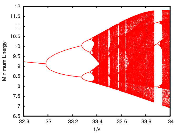
a) Period doubling cascade	b) $1/\nu=33.2701$
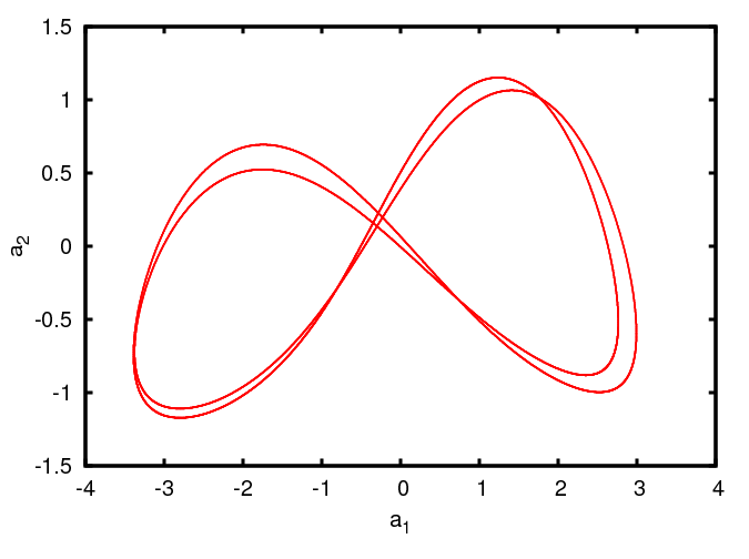
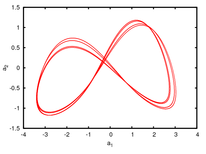
c) $1/\nu=33.3353$	d) $1/\nu=33.3569$

Figure 1: Figure a) shows a period-doubling bifurcation cascade. Figures b) to d) show the projection on the $a_{1}-a_{2}$ coordinates of some periodic orbits of the first three period-doublings.

Remark 1.1.

The period doubling cascades described above have, to the limit of numerical precision, the same quantitative properties than the one-dimensional ones found in [17, 45] even if the K-S, in principle, is an infinite dimensional dynamical system. Nevertheless, since the system admits an inertial manifold it is plausible that the arguments of [10] apply.

The papers [30, 31, 12] present a very remarkable explicit surface of section which allows to reduce approximately to a one dimensional map. Other sources of periodic orbits can be found as a byproduct of computations of inertial manifolds [27, 22, 37, 28, 14]. In this paper we will not use these methods, but the periodic orbits found by them could be validated using the methods here.

2 Derivation of the invariance equation for the periodic orbits.

Here we derive a functional equation for the periodic orbits of the Kuramoto-Sivashinsky equation. This functional equation is well suited for applying a fixed point problem for a well-defined operator. Later on, with this equation, we develop a numerical scheme for the computation of these orbits and an a posteriori verification method.

Periodic orbits with period $T$ of the Kuramoto-Sivashinsky equation (1) satisfy, under the time rescaling $\theta=\dfrac{2\pi t}{T}$, the invariance equation

$$f\partial_{\theta}u+Lu+\frac{1}{2}\partial_{x}\left(u^{2}\right)=0,$$ (4)

where $L=\nu\partial_{x}^{4}+\partial_{x}^{2}$ and $f=\frac{2\pi}{T}$. A solution of Equation (4) is represented by a pair $(f,u)$, where $f$ is a real number and $u:\mathbb{T}^{2}\rightarrow\mathbb{R}$, $u(\theta,x)$ is odd with respect $x$.

Given an approximate solution $(f_{0},u_{0})$ of Equation (4), we look for a correction $(\sigma,\delta)$ of it. This correction satisfies the equation

$$f_{0}\partial_{\theta}\delta+L\delta+\partial_{x}\left(u_{0}\cdot\delta\right)+\sigma\partial_{\theta}u_{0}=-e-\frac{1}{2}\partial_{x}(\delta^{2})-\sigma\partial_{\theta}\delta,$$ (5)

where $e=f_{0}\partial_{\theta}u_{0}+Lu_{0}+\frac{1}{2}\partial_{x}(u_{0}^{2})$ is the error of the approximation $(f_{0},u_{0})$.

Equation (5) has two problems:

1. Solutions of Equation (4) are non-unique: If $(\sigma,\delta(\theta,x))$ is a solution, then so is $(\sigma,\delta(\theta+a,x))$, $\forall a\in\mathbb{R}.$

2. The linear part of Equation (5) is an unbounded operator. This leads to numerical instabilites.

To fix the non-uniqueness problem, we impose another equation so that Problem (5) has a unique solution.

To motivate the choice of normalization, we observe that if $u(\theta,x)$ is a solution of Equation (4) satisfying

$$\int_{\mathbb{T}^{2}}u\cdot\partial_{\theta}u=C\text{ (Constant)}.$$ (6)

Then, a translation in the $\theta$ direction – the source of non-uniqueness changes the quantity (6) by

$$\int_{\mathbb{T}^{2}}u(\theta+a,x)\cdot\partial_{\theta}u(\theta,x)\simeq\int_{\mathbb{T}^{2}}(u(\theta,x)+\partial_{\theta}u(\theta,x)a)\cdot\partial_{\theta}u(\theta,x)=C+a\|\partial_{\theta}u\|^{2}_{L^{2}(\mathbb{T}^{2})}.$$

Thus,

$$\int_{\mathbb{T}^{2}}u(\theta+a,x)\cdot\partial_{\theta}u(\theta,x)=C+a\|\partial_{\theta}u\|^{2}_{L^{2}(\mathbb{T}^{2})}+O(a^{2}).$$

The above calculation can be interpreted geometrically saying that the surface in function space given by (6) is transversal to the symmetries of the equation.

Therefore, we impose local uniqueness for Equation (5) by requiring that the correction $\delta$ should be perpendicular to the approximate parameterization $u_{0}$. That is,

$$\int_{\mathbb{T}^{2}}\delta\cdot\partial_{\theta}u_{0}=0.$$

As we observed before, the linear operator $f_{0}\partial_{\theta}+L$ is unbounded, but we can transform Equation (5) into a smooth equation by performing algebraic manipulations. Let $c\in\mathbb{R}$ be such that $S_{c}=f_{0}\partial_{\theta}+L+c{\rm Id}$ is invertible. Then, we have that $(\sigma,\delta)$ in Equation (5) satisfies the equation

$$A\begin{pmatrix}\sigma\\ \delta\end{pmatrix}=\tilde{e}+\tilde{N}\begin{pmatrix}\sigma\\ \delta\end{pmatrix},$$

where

$$A=\begin{pmatrix}0&\int_{\mathbb{T}^{2}}\cdot\partial_{\theta}u_{0}\\ S_{c}^{-1}\partial_{\theta}u_{0}&{\rm Id}-cS_{c}^{-1}+S_{c}^{-1}\partial_{x}(u_{0}\cdot)\\ \end{pmatrix},$$ (7)

$$\tilde{e}=\begin{pmatrix}0\\ -S_{c}^{-1}e\end{pmatrix},$$

and

$$\tilde{N}\begin{pmatrix}\sigma\\ \delta\end{pmatrix}=-S_{c}^{-1}\left(\frac{1}{2}\partial_{x}(\delta^{2})+\sigma\partial_{\theta}\delta\right).$$

2.1 Algorithm for computing periodic orbits.

From the discussion in Section 2, we have that our solution $z=(\sigma,\delta)$ satisfies a functional equation of the form

$$Az=\tilde{e}+\tilde{N}(z,z),$$ (8)

where $A$, given by Equation (7), is a bounded linear operator and $\tilde{N}$ is the nonlinear part ($N(0)=DN(0)=0$).

The Newton scheme is based on solving Equation (8) numerically. Given an initial guess $(f_{0},u_{0})$, we update it by finding the correction $z=(\sigma,\delta)$ that is a solution of the linear equation

$$Az=\tilde{e},$$ (9)

and obtain $(f_{1},u_{1})=(f_{0}+\sigma,u_{0}+\delta)$. This process is repeated several times until a stopping criterion, $\|\tilde{e}(f_{k},u_{k})\|<tol$, is fullfilled. As in all Newton’s methods, if $(f_{k},u_{k})$ is an approximate solution, then at each step the error decreases quadratically, $\|\tilde{e}(f_{k+1},u_{k+1})\|\approx\|\tilde{e}(f_{k},u_{k})\|^{2}$. Since the problem is infinite dimensional, truncation to the most significatives Fourier modes is required. This transforms the problem to a finite dimensional one.

Summarizing, we obtain the following algorithm:

Algorithm 1.

• • An approximate solution $(f_{0},u_{0})$ of the invariance equation (4).

  • The accuracy tol for the computation of the solution. This gives an upper bound of the accuracy of the outputs of the algorithm.

• An approximate solution $(f_{k},u_{k})$ of the invariance equation with tolerance less than tol.

• Fix a norm on the space of periodic functions on the torus (see Appendix A for examples of such norms).

• Set $k=0$.

• Compute the error $\tilde{e}_{k}=-S_{c}^{-1}\left(f_{k}\partial_{\theta}u_{k}+Lu_{k}+\frac{1}{2}\partial_{x}(u_{k}^{2})\right)$.

• If $\|\tilde{e}_{k}\|<\text{\bf tol}$ stop the algorithm. The pair $(f_{k},u_{k})$ is the approximation of the frequency and the periodic orbit with the desired accuracy.

• Solve the (finite dimensional truncated) linear system (9) by means of a linear solver, obtaining the solution pair $(\sigma,\delta)$.

• Set $u_{k+1}=u_{k}+\delta_{k}$, $f_{k+1}=f_{k}+\sigma_{k}$, and update $k$ with $k+1$.

• If $\|(\sigma,\delta)\|<\text{\bf tol}$, stop the algorithm. The pair $(f_{k+1},u_{k+1})$ is the approximation of the periodic orbit and its frequency with the desired accuracy. Otherwise, repeat the process starting from step 1).

Remark 2.1.

As said before, all computations are performed by representing all Fourier series as Fourier polynomials of order, say, $N$. However, we notice that in Step 1), where the error $\tilde{e}_{k}$ is computed, the computation of $u^{2}$ is required, hence, when we apply the functional to a polynomial of degree $N$, we obtain a polynomial of degree $2N$. We have observed in our numerical tests that a way to obtain sharp estimates is to compute the functional with $2N$ coefficients. By doing so the bounds obtained by the algorithm are very sharp and suitable for the validation scheme presented in Section 4.

2.2 Computation of the stability of a periodic orbit.

Once a periodic orbit $(f,u)$ is computed one often desires to compute its stability (the dimension of the unstable manifold). One way of computing it is counting the number of eigenvalues of the Floquet operator that are outside the unit circle. That is, integrate the linear differential equation

$$f\partial_{\theta}v=-Lv-\partial_{x}(u\cdot v)$$

with initial condition $v_{0}={\rm Id}$, up to time $1$, and compute the spectrum of $v_{1}$. Then, check how many eigenvalues are outside the unit disk. Of course, this should be done by truncating all computations in finite dimensions and bounding the errors.

Another way is computing the spectrum of the unbounded (but closed) linear operator

$$f\partial_{\theta}+L+\partial_{x}(u\cdot).$$ (10)

Given an eigenvalue $\lambda$ of the Floquet operator, $\log(\lambda)+if\cdot n$, $n\in\mathbb{Z}$, is an eigenvalue of the operator (10). Hence, restricting the spectrum on a set of the form $\Gamma_{a}=\{z\in\mathbb{C}:a\leq\text{Im}(z)<a+f\}$ is in one-to-one correspondence with the spectrum of the Floquet operator. In particular, computing the dimension of the unstable manifold is the same as computing the number of eigenvalues of the operator (10) restricted to the left half-plane $\Gamma_{a}\bigcap\{z:\text{Im}(z)<0\}$.

Even if the two methods are equivalent for the equations that define a differentiable flow, we note that the method based on studying the spectrum of (10) makes sense even in equations that do not define a flow. Hence, this is the method that we will use.

3 An a posteriori theorem for the rigorous verification of the existence of periodic orbits.

In this section we present an a posteriori result, Theorem 3.1 that, given an approximate solution $(f,u)$ of Equation (4) satifying some explicit quantitative assumptions, ensures the existence of a true solution of (4) and estimates the distance between this true solution and the approximate one. Of course, the solutions of (4) give periodic solutions of the evolution equation. Theorem 3.1 is a tailored version of Theorem 2.3 apprearing in [19]. For the sake of completeness, we will state it here adapted to Equation (8). Note that the theorem is basically an elementary contraction mapping principle, but that we allow for the application of a preconditioner, which makes it more applicable in practice.

Theorem 3.1.

Consider the operator

$$F(z)=Az-\tilde{e}-N_{{\bar{u}}}(z),$$ (11)

defined in $\overline{B_{{\bar{u}}}(\rho)}=\{u:\|u-{\bar{u}}\|\leq\rho\}$, with $\rho>0$, and where $N_{{\bar{u}}}$ the nonlinear part of the operator $F$ at the point ${\bar{u}}$, that is

$$N_{{\bar{u}}}(z)=F({\bar{u}}+z)-F({\bar{u}})-DF({\bar{u}})z.$$

Let $B$ be a linear operator such that $BDF({\bar{u}})$, $BF$ and $BN_{{\bar{u}}}$ are continuous operators. If, for some $b,K>0$ we have:

1. $\|I-BDF({\bar{u}})\|=\alpha<1$.

2. $\|B\left(F({\bar{u}})+N_{{\bar{u}}}(z)\right)\|\leq b$ whenever $\|z\|\leq\rho$.

3. $\text{Lip}_{\|z\|\leq\rho}BN_{{\bar{u}}}(z)<K$

4. $\frac{b}{1-\alpha}<\rho$.

5. $\frac{K}{1-\alpha}<1$.

then there exists $\delta u$ such that ${\bar{u}}+\delta u$ is in $\overline{B_{{\bar{u}}}(\rho)}$ and is a unique solution of Equation (11), with $\|\delta u\|\leq\frac{\|BF({\bar{u}})\|}{1-\alpha-K}$.

We are now in a position to write down the theorem for the existence and local uniqueness of periodic orbits and their period for the Kuramoto-Sivashinsky equation. This theorem has been written for the special case of the family of Banach spaces $X_{M}$, that depends on the parameters $r,s_{1},s_{2}\geq 0$. It is the Banach space of periodic functions $u(\theta,x)=\sum_{(k_{1},k_{2})\in\mathbb{Z}^{2}}u_{k_{1},k_{2}}e^{i(k_{1}\cdot x+k_{2}\cdot\theta)}$ with finite norm

$$\|u\|_{M}=\sum_{(k_{1},k_{2})\in\mathbb{Z}^{2}}M(k_{1},k_{2})|u_{k_{1},k_{2}}|,$$

where

$$M(k_{1},k_{2})=(1+|k_{1}|)^{s_{1}}(1+|k_{2}|)^{s_{2}}e^{r(|k_{1}|+|k_{2}|)}.$$

When there is no confusion, we will denote the norm by $\|\cdot\|_{M}$. These spaces have the property that all their elements are analytic functions for $r\neq 0$. See Appendix A for a more detailed discussion.

Theorem 3.2.

Let $r,s_{1},s_{2}\geq 0$ define the Banach space $X_{M}$, and $(f,u)$ be an approximate solution of Equation (4), with error $e$, and consider Equation (8) for the correction $(\sigma,\delta)$. Let $B={\rm Id}+\hat{B}$ be a linear operator, and suppose that the following conditions are satisfied:

1. $\|\hat{B}\hat{A}+\hat{A}+\hat{B}\|_{M}=\alpha<1$,

2. $\|B\|_{M}\|\tilde{e}\|_{M}\leq e_{1}$,

3. $\|B\|_{M}(\|S_{c}^{-1}\partial_{\theta}\|_{M}+\frac{1}{2}\|S_{c}^{-1}\partial_{x}\|_{M})\leq e_{2}$,

4. $(1-\alpha)^{2}-4e_{1}e_{2}>0$,

then there exists a solution $z_{*}=(\sigma_{*},\delta_{*})$ of Equation (8) satisfying $\|z_{*}\|_{M}\leq E=\frac{e_{1}}{1-\alpha-\rho_{-}}$, where $\rho_{-}=1-\alpha-\sqrt{(1-\alpha)^{2}-4e_{1}e_{2}}$.

Proof.

Let $\rho>0$ such that $1-\alpha-\sqrt{(1-\alpha)^{2}-4e_{1}e_{2}}<2e_{2}\rho<1-\alpha$. We need to deduce all the conditions in Theorem 3.1. Notice that $z=(\sigma,\delta)$ and $Q(z,z)=S_{c}^{-1}(\sigma\partial_{\theta}\delta+\frac{1}{2}\partial_{x}(\delta^{2}))$. Condition 1) in Theorem 3.1 is the same as condition a) for the present theorem.

$b$ in condition b) is $e_{1}+e_{2}\rho^{2}$, because if $\|(\sigma,\delta)\|_{M}\leq\rho$, then

$$\begin{split}&\left\|B\left(\tilde{e}+S_{c}^{-1}(\sigma\partial_{\theta}\delta+\frac{1}{2}\partial_{x}(\delta^{2}))\right)\right\|_{M}\leq\|B\|_{M}\|\tilde{e}\|_{M}+\|BS_{c}^{-1}(\sigma\partial_{\theta}\delta+\frac{1}{2}\partial_{x}(\delta^{2}))\|_{M}\\ &\phantom{AAAAA}\leq e_{1}+\|BS_{c}^{-1}(\sigma\partial_{\theta}\delta)\|_{M}+\frac{1}{2}\|BS_{c}^{-1}(\partial_{x}(\delta^{2}))\|_{M}\\ &\phantom{AAAAA}\leq e_{1}+\|B\|_{M}\left(\|S_{c}^{-1}\partial_{\theta}\|_{M}|\sigma|\|\delta\|_{M}+\frac{1}{2}\|S_{c}^{-1}\partial_{x}\|_{M}\|\delta\|^{2}_{M}\right)\\ &\phantom{AAAAA}\leq e_{1}+e_{2}\rho^{2}.\end{split}$$

$K$ in condition c) is $2e_{2}\rho$ because if $\|z\|_{M},\|\hat{z}\|_{s_{1},s_{2}}\leq\rho$, then

$$\begin{split}\|B\left(Q(z,z)-Q(\hat{z},\hat{z})\right)\|_{M}\\ \leq\|B\|_{M}\|S_{c}^{-1}\left(\sigma\partial_{\theta}\delta-\hat{\sigma}\partial_{\theta}\hat{\delta}+\delta\partial_{x}\delta-\hat{\delta}\partial_{x}\hat{\delta}\right)\|_{M}\\ \phantom{AA}\leq\|B\|_{M}\left(\|S_{c}^{-1}(\sigma\partial_{\theta}(\delta-\hat{\delta})+(\sigma-\hat{\sigma})\partial_{\theta}\hat{\delta})\|_{M}+\|S_{c}^{-1}(\delta\partial_{x}(\delta-\hat{\delta})+(\delta-\hat{\delta})\partial_{x}\hat{\delta})\|_{M}\right)\\ \phantom{AA}\leq\|B\|_{M}\left(\|S_{c}^{-1}\partial_{\theta}\|_{M}+\frac{1}{2}\|S_{c}^{-1}\partial_{x}\|_{M}\right)2\rho\|z-\hat{z}\|_{M}\\ \phantom{AA}\leq 2e_{2}\rho\|z-\hat{z}\|_{M}.\end{split}$$

Conditions d) and e) of Theorem 3.1 are equivalent to

$$\frac{2e_{2}\rho}{1-\alpha}<1\text{ \quad and \quad}\frac{e_{1}+e_{2}\rho^{2}}{1-\alpha}<\rho,$$

which are satisfied because $1-\alpha-\sqrt{(1-\alpha)^{2}-4e_{1}e_{2}}<2e_{2}\rho<1-\alpha$.

Finally, the upper bound on the norm on the solution $\|z_{*}\|_{M}$ is obtained by applying Theorem 3.1 with ${\rho=\frac{1-\alpha-\sqrt{(1-\alpha)^{2}-4e_{1}e_{2}}}{2e_{2}}}$. ∎

Remark 3.3.

Notice that, using the radii polynomial approach, we obtain that $\alpha,e_{2}$ are functions of the radius $\rho$. Therefore, we obtain a range of radii for which Theorem 3.1 applies. Of course the largest radius is a better result for the uniquess part and the smallest radius is a better result fof the distance to the initial guess

4 Implementation of the rigorous computer assisted validation of periodic orbits for the Kuramoto-Sivashinsky equation.

We use Theorem 3.2 and construct an implementation of the computer assisted validation of periodic orbits. Our initial data, $(f,u)$, will consist of a real number $f$, a trigonometric polynomial $u$ of degrees $(d_{1},d_{2})$ in the variables $(\theta,x)$, and the operator $B={\rm Id}+\hat{B}$, where $\hat{B}$ is a $2d_{1}\cdot(2d_{2}+1)\times 2d_{1}\cdot(2d_{2}+1)$ dimensional matrix (this operator can be obtained by nonrigorous computations by approximating the inverse of the operator $A$).

First of all, notice that the constants $e_{1}$ and $e_{2}$ in Theorem 3.2 depend on the diagonal operators $S_{c}^{-1}$, $\partial_{\theta}$ and $\partial_{x}$, and on the norms of $B$ and $\tilde{e}$. The computation of the norms of the (diagonal) operators $S_{c}^{-1}\partial_{\theta}$ and $S_{c}^{-1}\partial_{x}$, is done in Appendix A, lemma A.5.

Secondly, the computation of the norms of the operator $B$ and the error $\tilde{e}$ can be done with the help of computer assisted techniques because they are finite dimensional: $\tilde{e}$ is a trigonometric polynomial of dimension $2d_{1}\cdot(2d_{2}+1)$ and $B={\rm Id}+\hat{B}$ implies that $\|B\|_{M}\leq 1+\|\hat{B}\|_{M}$ ( Note that $\|\hat{B}\|_{M}$ is the norm of a finite dimensional matrix).

Finally, it remains to show how to compute operator norm of

$$\|\hat{B}\hat{A}+\hat{A}+\hat{B}\|_{M}.$$ (12)

Since $u$ is a trigonometric polynomial, the operator $\hat{A}$ is a band operator: $\hat{A}_{i,j}=0$ for $|i|>d_{1}$ or $|j|>2d_{2}+1$. Hence $\hat{A}$ decomposes as the sum of a finite matrix $\hat{A}_{F}$ of dimensions $2d_{1}\cdot(2d_{2}+1)\times 2d_{1}\cdot(2d_{2}+1)$ and a linear operator $\hat{A}_{I}$. This operator $\hat{A}_{I}$ is:

$$\hat{A}_{I}=\mathbb{P}_{(>d_{1},>d_{2})}\left(-cS_{c}^{-1}+S_{c}^{-1}\partial_{x}(u\cdot)\right)=-c\mathbb{P}_{(>d_{1},>d_{2})}S_{c}^{-1}\mathbb{P}_{(>d_{1},>d_{2})}+\mathbb{P}_{(>d_{1},>d_{2})}S_{c}^{-1}\partial_{x}\mathbb{P}_{(>d_{1},>d_{2})}(u\cdot),$$ (13)

where $\mathbb{P}_{(\leq d_{1},\leq d_{2})}$ is the projection operator on the $d_{1}\cdot(d_{2}+1)$-dimensional vector space spanned by the low frequencies and $\mathbb{P}_{(>d_{1},>d_{2})}={\rm Id}-\mathbb{P}_{(\leq d_{1},\leq d_{2})}$.

Hence,

$$\|\hat{B}\hat{A}+\hat{A}+\hat{B}\|_{M}\leq\max\left\{\|\hat{B}\hat{A}_{F}+\hat{A}_{F}+\hat{B}\|_{M},\|{\rm Id}+\hat{B}\|_{M}\|\hat{A}_{I}\|_{M}\right\}.$$ (14)

Remark 4.1.

Notation $\mathbb{P}_{(>d_{1},>d_{2})}$ could be a little bit misleading: It does not mean that it is the projection operator on the high frequencies for both variables, but the complementary of the low frequencies projection operator.

The norm $\|\hat{B}\hat{A}_{F}+\hat{A}_{F}+\hat{B}\|_{M}$ appearing in the upper bound (14) can be estimated with the help of computer assisted techniques, while the norm $\|{\rm Id}+\hat{B}\|_{M}\|\hat{A}_{I}\|_{M}$ is split into the computation of $\|{\rm Id}+\hat{B}\|_{M}$ and $\|\hat{A}_{I}\|_{M}$. The former is done as said before, while the latter (the bound of the operator (13)) is bounded above by:

$$cK_{1}+K_{2}K_{3},$$ (15)

where $K_{1}=\|\mathbb{P}_{(>d_{1},>d_{2})}S_{c}^{-1}\mathbb{P}_{(>d_{1},>d_{2})}\|_{M}$, $K_{2}=\|\mathbb{P}_{(>d_{1},>d_{2})}S_{c}^{-1}\partial_{x}\mathbb{P}_{(>d_{1},>d_{2})}\|_{M}$ and $K_{3}=\|u\|_{M}$. Fixing $c=\frac{1}{\nu}$ and with the help of Lemma A.4 we obtain that

$K_{1}=\sqrt{2}\max\left\{\max_{x>d_{1}}\left\{\dfrac{1}{p(x)}\right\},\dfrac{1}{f(d_{2}+1)}\right\},$

$K_{2}=\sqrt{2}\left(\frac{4}{3\nu}\right)^{\frac{1}{4}}\left(\max\left\{\max_{x>d_{1}}\left\{\dfrac{1}{p(x)}\right\},\dfrac{1}{f(d_{2}+1)}\right\}\right)^{\frac{3}{4}},$

$K_{3}=\sup_{(i_{1},i_{2})\in\mathbb{Z}^{2}}|u_{i_{1},i_{2}}|M(i_{1},i_{2}).$

Remark 4.2.

Since $u$ is a trigonometric polynomial, $K_{3}$ is in fact computed by

$$\sup_{(i_{1},i_{2})\in[0,2d_{1}+1]\times[1,2d_{2}+1]}|u_{i_{1},i_{2}}|M(i_{1},i_{2}).$$

Remark 4.3.

The upper bound given in lemma A.4 tends to zero as the number of modes used in the discretization tends to infinity. This assures us that this methodology is reliable.

Remark 4.4.

The computation of the norm (12) is very demaning in terms of computer power effort. Fortunately, not very sharp results are needed. Provided that we can prove that the norm is less than $1$, we obtain a contraction. The final result is not too afected by the contraction factor. On the other hand, the bound on the error $e_{1}$ in Theorem 3.2 has a very direct influence in the error established.

Hence, a good strategy is to perform the matrix computations with the lowest dimensions possible and perform the estimate of $e_{1}$ with the highest possible number of modes. This relies on the fact that given two functions $u_{0}$ and $u_{1}$ with $\|u_{0}-u_{1}\|_{M}\leq\delta$, then their associated $\hat{A}_{u_{i}}$ satisfy that $\|\hat{A}_{u_{0}}-\hat{A}_{u_{1}}\|_{M}\leq\|S_{c}^{-1}\partial_{x}\|_{M}\delta\leq K_{2}\delta$. This strategy is reflected in Algorithm 2.

One should also realize that the calculation of the operator $B$ does not need to be justified. Some further heuristic approximations that reduce the computational effort could be taken (e.g. a Krylov method that gives a finite rank approximation). We have not taken advantage of this possibilities since they were not needed in our case.

Finally, we note that since the preconditioner is not so crucial, and it is more expensive to compute, in continuation algorithms, it could be good to update it less frequently than the residual.

Now in a position of giving the algorithm for the validation of the existence and local uniqueness of periodic orbits near a given approximate one $(f,u)$. We suppose that the approximation is obtained by the methods explained in Section 2.1.

Remark 4.5.

For more details on the computer implementation of this algorithm (e. g. the rigorous manipulation of Fourier series), we refer to the appendix in [18] or [24].

Algorithm 2.

• • $r,s_{1},s_{2}\geq 0$, defining the Banach space $X_{M}$.

  • An approximate solution $(f,u)$ to Equation (4), of dimensions $d_{1},d_{2}$ in the variables $t,x$.

  • A pair of natural numbers $\tilde{d}_{1},\tilde{d}_{2}$ such that $\tilde{d}_{i}\leq d_{i}$, $i=1,2$.

• If succeeded, the existence of a constant $\rho_{-}>0$ where a (unique) solution of the invariance equation exists inside the ball centered at $(f,u)$ with radius $\rho_{-}$.

• Compute the trigonometric polynomial $\tilde{u}$ by truncating $u$ up to $\tilde{d}_{1},\tilde{d}_{2}$.

• Compute an upperbound $\delta$ of $\|\tilde{u}-u\|_{M}$.

• Compute the matrix $\hat{A}_{F}$ and the matrix $\hat{B}$ associated to $\tilde{u}$.

• Compute an upper bound, $\alpha_{1}$, of $\|\hat{B}\hat{A}_{F}+\hat{B}+\hat{A}_{F}\|_{M}.$

• Compute upper bounds of the constants $K_{1},K_{2}$ and $K_{3}$.

• Compute an upper bound, $\alpha_{2}$, of $cK_{1}+K_{2}K_{3}$.

• Compute an upper bound, $b$, of $1+\|\hat{B}\|_{M}$.

• Compute $\alpha=\max\{\alpha_{1},\alpha_{2}\}+K_{2}\delta b$. If $\alpha$ is greater than $1$ then the algorithm stops and the result is that the validation has failed, otherwise continue with Step 7).

• Compute an upper bound, $e_{0}$, of $\|\tilde{e}\|_{M}$.

• Compute an upper bound, $e_{1}$, of $b\cdot e_{0}$.

• Compute an upper bound, $e_{2}$, of $b\cdot(\|S_{c}^{-1}\partial_{\theta}\|_{M}+\frac{1}{2}\|S_{c}^{-1}\partial_{x}\|_{M})$.

• Check if $(1-\alpha)^{2}-4e_{1}e_{2}>0$.

If the inequality in 12) is true then, by Theorem 3.2, there exists a unique periodic orbit $(f_{*},u_{*})$ such that $\|(f_{*}-f,u_{*}-u)\|_{M}\leq E=\dfrac{e_{1}}{1-\alpha-\rho_{-}}$, where $\rho_{-}$ has the expression as in Theorem 3.2.

Remark 4.6.

The computation of the product of the interval matrices $\hat{B}$ and $\hat{A}_{F}$ is the bottleneck, in terms of computational time, of the algorithm: naive multiplication of the matrices leads to disastrous speed results. To speed up this we use the techniques in [41, 38], which describe algorithms for the rigorous computation of product of interval matrices with the help of the BLAS package. See Appendix B for a presentation of this technique.

4.1 Improving the radius of analyticity of solutions

A simple strategy for giving rigorous lower bounds of the analyticity radius of the solutions is by first performing Algorithm 2 with $r\approx 0$. Then, apply a posteriori bounds for improving the value of $r$. (See [25] for an application of this technique in the context of ODEs).

Denote by $\alpha_{r}$, $e_{1,r},$ and $e_{2,r}$ the upperbounds appearing in Theorem 3.2 when computed with the one-parametric norm $\|\cdot\|_{M_{r}}$ (the weight $M_{r}$ depends on the radius of analyticity). Moreover, notice that for any trigonometric polynomial $u$ of dimensions $d_{1}\times d_{2}$ and for any $\hat{r}>0$ we have $\|u\|_{M_{\hat{r}}}\leq\|u\|_{M_{0}}e^{\hat{r}d_{1}d_{2}}$ and for any finite dimensional $A$ of dimensions $d\times d$ $\|T\|_{M_{\hat{r}}}\leq\|T\|_{M_{0}}e^{\hat{r}d}$. Hence, since the application of Theorem 3.2 is performed with finite dimensional approximations we obtain that $\alpha_{\hat{r}}\leq\alpha_{0}e^{\hat{r}d_{1}d_{2}}$, $e_{1,\hat{r}}\leq e_{1,0}e^{2\hat{r}d_{1}d_{2}}$ and $e_{2,\hat{r}}\leq e_{2,0}e^{\hat{r}d_{1}d_{2}}$. So, by imposing that these upperbounds satisfy the conditions appearing in Theorem 3.2 we obtain larger values of the radius of analyticity of the solutions.

Of course, some more detailed results could be obtained by repeating the calculation of the norms in the spaces of analytic spaces closer to the true value. Of course, this will require reduing all the estimates of norms.

The analyticity properties of solutions of K-S equations have been studied rigorously in [9, 23] and it is shown to have thermodynamicas properties and relations with the number of zeros, determining modes, etc.

5 Some numerical examples.

In this section we present some examples of the methods developed in Section 2.1 for the computation of periodic orbits and in Section 4 for the a posteriori verification of them.

5.1 Example of numerical computation. Period doubling.

We have continued some branches of the doubling period bifurcation diagram, shown in Subfigure a) in Figure 1. This has been done by first computing some of the attracting orbits by integration, see Section 1. These periodic orbits have been used as seeds for our numerical algorithm.

Specifically, for the values of the parameter $\frac{1}{\nu}$ equal to $32.9$, $33.1$ and $33.3$ we have computed 3 (attracting) periodic orbits at the first 3 stages of the period doubling cascades. Then, for each one of them, we have continued them with our numerical algorithm. With the help of Algorithm 1 we have been able to cross the period doubling bifurcations, where the attracting orbits bifurcate to a doubled period one (that is attracting) and to an unstable one. Our continuations are able to continue these unstable orbits. See Figure 2 for a representation of these orbits in the period doubling cascade diagram and Figure 3 for the representation of two of these orbits.

The computational time of its validation takes no more than 30 seconds in a single 2.7 GHz CPU of a regular laptop. We hope that thid could be used in the catalogue of periodic orbits computed in [31]. Note that, of course, validating different peridic orbits is verily easily paralellizable.

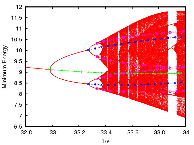
Figure 2: The continuation of the first 3 periodic orbits on the period doubling cascade. These are superposed to the period doubling cascade using three different colors.

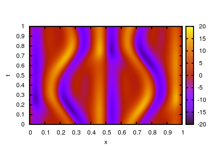
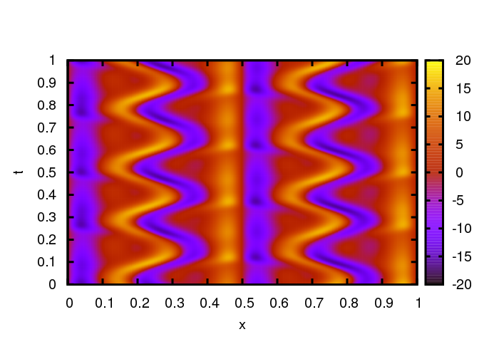
$1/\nu=33.27$. Period $=0.89893314191428$.	$1/\nu=33.5069$. Period $=3.49489164733297$.

Figure 3: Representation of two periodic orbits computed with the Newton method. Colors represent the value of the orbit $u$ at the $(\theta,x)$ coordinate.

5.2 Example of a validation.

With the help of the algorithm presented in Section 4 (and with the improvment trick explained in Subsection 4.1) we can validate the existence of some periodic orbits. For example, we validate the existence of a periodic orbit with $\frac{1}{\nu}=32.97$. The approximate data is given by $40$ $x$ modes and $(2\cdot 19+1)$ $t$ modes. The approximate period is $0.895839$. The validation has been done with the finite matrix $\hat{B}$ with dimension 6994, and with $r=s_{1}=s_{2}=1\cdot 10^{-12}$.

The output of the validation is:

• The error produced by the approximate periodic orbit is $\|S^{-1}_{c}\varepsilon\|_{M}\leq 8.489632\cdot 10^{-10}$.

• $K_{1}\leq 8.189680\cdot 10^{-3}$ , $K_{2}\leq 6.332728\cdot 10^{-2}$ , $K_{3}\leq 6.693947$ .

• The error of the tails of the operator $\hat{A}$ is less than or equal to $K_{1}\cdot c+K_{2}\cdot K_{3}=6.946684\cdot 10^{-1}$.

• The norm of the approximate inverse of the linear operator $Id+\hat{A}$ is $\|\text{Id}+\hat{B}\|_{M}=4.567111\cdot 10^{1}$.

• $\|\hat{B}+\hat{A}+\hat{B}\cdot\hat{A}\|_{M}=6.716849\cdot 10^{-14}$

• $\alpha=\|\text{Id}+\hat{B}+\hat{A}+\hat{B}\hat{A}\|_{M}=6.946684\cdot 10^{-1}$

• $(1-\alpha)^{2}-4e_{1}e_{2}=9.321303\cdot 10^{-2}$

As a result of the validation we obtain that the distance of the true periodic orbit to the approximate solution is less than or equal to $1.269966\cdot 10^{-7}$.

The computational time of one of these validations is no more than 1017 seconds in a single 2.7 GHz CPU on a regular laptop.

Other validation results for other periodic orbits is shown in table 1.

$\frac{1}{\nu}$	Period	$E$	Improved radius of analyticity	Improved $E$
$8.199953$	$2.992730$	$2.463363\cdot 10^{-11}$	$1.512026\cdot 10^{-4}$	$1.002122\cdot 10^{-9}$
$8.230453$	$3.074450$	$4.385135\cdot 10^{-11}$	$1.268306\cdot 10^{-4}$	$6.199587\cdot 10^{-9}$
$31.00000$	$0.806901$	$8.642523\cdot 10^{-10}$	$9.154580\cdot 10^{-5}$	$1.043836\cdot 10^{-8}$
$32.97000$	$0.895839$	$1.269966\cdot 10^{-7}$	$1.101236\cdot 10^{-4}$	$2.902773\cdot 10^{-6}$
$33.27010$	$0.881170$	$1.049117\cdot 10^{-7}$	$1.120727\cdot 10^{-4}$	$4.092897\cdot 10^{-6}$

Table 1: Validation results of some periodic orbits for different values of the parameter $\nu$. The columns show: $\frac{1}{\nu}$, the period of the periodic orbit, the radius of the ball obtained from Theorem 3.2 computed with the norm $\|\cdot\|_{M}$ with $s_{1}=s_{2}=10^{-12}$ and $r=10^{-12}$, the improved radius of analyticity obtained applying the trick explained in Remark 4.1, and the new radius of the ball obtained from Theorem 3.2 computed with the norm $\|\cdot\|_{M}$ with $s_{1}=s_{2}=10^{-12}$ and $r$ equal to the value in fourth column. All validation took around 1000 seconds in a single 2.7 GHz CPU on a regular laptop. Some of the periodic orbits that appear in this table appear also in [47].

Appendix A $L^{1}$ weighted spaces of periodic functions.

In this section we develop the theoretical framework developed in [19] for some concrete spaces. The spaces have been chosen have the properties that they can encode analytic functions, the norms are easily computable from Fourier series, have Banach algebra properties and the norms of linear operators can be estimated easily from the matrix elements. A technical, but sometimes useful property is that the dual is also a sequence space so that all the functionals are represented by its matrices (that is, there are no functionals at infinity. See [21] for examples and results on spaces based on $L^{\infty}$ which have functionals at infinity such as the taking the limit).

From now on, all norms of vectors in finite dimensional vector spaces will be the $L^{1}$-norm, in particular, the norm of a complex number is $|a+bi|=|a|+|b|$.

Let $X_{M}$, $r,s_{1},s_{2}\geq 0$, be the Banach space of periodic functions $u(\theta,x)=\sum_{(k_{1},k_{2})\in\mathbb{Z}^{2}}u_{k_{1},k_{2}}e^{i(k_{1}\cdot x+k_{2}\cdot\theta)}$ with finite norm

$$\|u\|_{M}=\sum_{(k_{1},k_{2})\in\mathbb{Z}^{2}}M(k_{1},k_{2})|u_{k_{1},k_{2}}|,$$

where

$$M(k_{1},k_{2})=(1+|k_{1}|)^{s_{1}}(1+|k_{2}|)^{s_{2}}e^{r(|k_{1}|+|k_{2}|)}.$$

Usually the values of $r,s_{1},s_{2}$ are fixed. When there is no confusion, we will denote the norm by $\|\cdot\|_{M}$, otherwise we will remark the dependency on the parameters $r,s_{1},s_{2}$ by subscripts on the weight $M$ (e.g. $M_{r}$).

If $r>0$ then $X_{M}$ is a subspace of the analytic functions with complex band radius $r$. Also, if $s_{1}\leq s_{1}^{\prime}$, $s_{2}\leq s_{2}^{\prime}$ and $r\leq r^{\prime}$, then $X_{M}\subset X_{M^{\prime}}$ and $\|u\|_{M}\leq\|u\|_{M^{\prime}}$.

Remark A.1.

For notational purposes, we present all the theory and analytic computations in $X_{M}$ with the complex exponential basis, even though all the periodic functions we work with are real. For accuracy efficiency, we implement our codes with the sine-cosine basis. That is, the periodic functions are represented as

$$u(\theta,x)=\sum_{k_{1}=1}^{\infty}\left(\sum_{k_{2}=0}^{\infty}a_{k_{1},k_{2}}\cos(k_{2}\theta)+b_{k_{1},k_{2}}\sin(k_{2}\theta)\right)sin(k_{1}x).$$

With this basis, the norm defined above is

$$\|u\|_{M}=\sum_{1\leq k_{1}<\infty,0\leq k_{2}<\infty}\left(|a_{k_{1},k_{2}}|+|b_{k_{1},k_{2}}|\right)M(k_{1},k_{2}).$$

For this choice of norm, all the estimates computed with the exponential basis remain valid with the sine-cosine basis.

$X_{M}$ is a Banach algebra, $\|u\cdot v\|_{M}\leq\|u\|_{M}\|v\|_{M}$. This is a consequence of the fact that the weight $M$ is submultiplicative, $M(k_{1}+l_{1},k_{2}+l_{2})\leq M(k_{1},k_{2})\cdot M(l_{1},l_{2})$.

If $T\colon X_{M}\rightarrow X_{M}$ is a linear operator with coefficients $\left\{T_{i,j}\right\}_{(i_{1},i_{2}),(j_{1},j_{2})\in\mathbb{Z}^{2}}$, then its norm is

$$\|T\|_{M}=\sup_{(j_{1},j_{2})\in\mathbb{Z}^{2}}\dfrac{\sum_{(i_{1},i_{2})\in\mathbb{Z}^{2}}|T_{(i_{1},i_{2}),(j_{1},j_{2})}|M(i_{1},i_{2})}{M(j_{1},j_{2})}.$$

Hence, for example, the norm of the multiplication operator $v\longrightarrow u\cdot v$ is

$$\sup_{(i_{1},i_{2})\in\mathbb{Z}^{2}}|u_{i_{1},i_{2}}|M(i_{1},i_{2}).$$ (16)

Remark A.2.

The norm in (16) is sharper than the norm estimates that used the property that $X_{M}$ is a Banach algebra.

Remark A.3.

These norms scale very well with respect the weights: Given a trigonometric polynomial $u$ of dimensions $d_{1}\times d_{2}$, and $\hat{r}>r$, then $\|u\|_{M_{\hat{r}}}\leq\|u\|_{M_{r}}e^{(\hat{r}-r)d_{1}d_{2}}$. Similarly, for a finite dimensional matrix $T$ of sizes $d\times d$, $\|T\|_{M_{\hat{r}}}\leq\|T\|_{M_{r}}e^{(\hat{r}-s)d}$.

A.1 Two lemmas for the validation algorithm.

The following two lemmas are using for the computation of some preliminary estimates for the validation algorithm in Section 4.

Lemma A.4.

Let $p(x)=\nu x^{4}-x^{2}+c$ and $S_{c}=f\partial_{\theta}+\nu\partial_{x}^{4}+\partial_{x}^{2}+c{\rm Id}$, with $c=\frac{1}{\nu}$. Then it is satisfied that

1. $$\|\mathbb{P}_{(>d_{1},>d_{2})}S_{c}^{-1}\mathbb{P}_{(>d_{1},>d_{2})}\|_{M}\leq\sqrt{2}\max\left\{\max_{x>d_{1}}\left\{\dfrac{1}{p(x)}\right\},\dfrac{1}{f(d_{2}+1)}\right\}.$$

2. $$\|\mathbb{P}_{(>d_{1},>d_{2})}S_{c}^{-1}\partial_{x}\mathbb{P}_{(>d_{1},>d_{2})}\|_{M}\leq\sqrt{2}\left(\frac{4}{3\nu}\right)^{\frac{1}{4}}\left(\max\left\{\max_{x>d_{1}}\left\{\dfrac{1}{p(x)}\right\},\dfrac{1}{f(d_{2}+1)}\right\}\right)^{\frac{3}{4}}.$$

Proof.

The first one follows from the fact that an upper bound of

$$\max_{x>d_{1}\text{ or }y>d_{2}}\dfrac{fy+p(x)}{(fy)^{2}+p(x)^{2}},$$

is a consequence of the inequalities

$$\begin{array}[]{ll}\dfrac{fy+p(x)}{(fy)^{2}+p(x)^{2}}\leq\dfrac{\sqrt{2}}{fy}&\\ \dfrac{fy+p(x)}{(fy)^{2}+p(x)^{2}}\leq\dfrac{\sqrt{2}}{p(x)}&\end{array}.$$

The second upper bound follows in a similar way as the first one but considering that

$$\begin{array}[]{l}\max_{x>d_{1}\text{ or }y>d_{2}}\dfrac{fy+p(x)}{(fy)^{2}+p(x)^{2}}x\\ \leq\max_{x>d_{1}\text{ or }y>d_{2}}\dfrac{fy+p(x)}{(fy)^{2}+p(x)^{2}}\frac{x}{p(x)^{\frac{1}{4}}}p(x)^{\frac{1}{4}}\\ \leq\left(\dfrac{4}{3\nu}\right)^{\frac{1}{4}}\max_{x>d_{1}\text{ or }y>d_{2}}\dfrac{fy+p(x)}{(fy)^{2}+p(x)^{2}}p(x)^{\frac{1}{4}}.\\ \end{array}$$

∎

Lemma A.5.

Let $p(x)=\nu x^{4}-x^{2}+c$ and $S_{c}=f\partial_{\theta}+\nu\partial_{x}^{4}+\partial_{x}^{2}+c{\rm Id}$, with $c=\frac{1}{\nu}$. Then it is satisfied that

1. $$\|S_{c}^{-1}\partial_{x}\|_{M}\leq\sqrt{2}\left(\frac{4}{3\nu}\right)^{\frac{1}{4}}.$$

2. $$\|S_{c}^{-1}\partial_{\theta}\|_{M}\leq\frac{\sqrt{2}}{f}.$$

Proof.

The first upper bound follows from the observation that

$$\dfrac{fy+p(x)}{(fy)^{2}+p(x)^{2}}x$$

is less than or equal to

$$\left(\frac{4}{3\nu}\right)^{\frac{1}{4}}\dfrac{fy+p(x)}{(fy)^{2}+p(x)^{2}}p(x)^{\frac{1}{4}}.$$

The second one is proved similarly.

∎

Appendix B Fast interval matrix multiplication algorithms.

The naive multiplication of two high dimensional ($\approx 5000\times 5000$) interval matrices is very inefficient. Here we present a fast algorithm that we have used for (rigorously) multiplying interval matrices. It is Algorithm 4.5 in [41].

The algorithm relies on a clever usage of the fast double floating point based matrix multiplication software BLAS [15]. It combines the fast algorithms in BLAS and rounding flags.

Let $\boldsymbol{A}=[A_{1},A_{2}]$ and $\boldsymbol{B}=[B_{1},B_{2}]$ be two interval matrices, where inside brackets we have written the lower and upper point matrices. (In bold letters we denote interval matrices, and in plain ones double matrices). The algorithm produces an interval matrix $\boldsymbol{C}=[C_{1},C_{2}]$ satisfying $\boldsymbol{A}\cdot\boldsymbol{B}\subseteq\boldsymbol{C}$.

Algorithm 3.

• Set the rounding up.

• Compute the double matrices:

  • $mA=(A_{1}+A_{2})/2$.

  • $rA=mA-A_{1}$.

  • $mB=(B_{1}+B_{2})/2$.

  • $rB=mB-B_{1}$.

  • $rC=|mA|\cdot rB+rA\cdot(|mB+rB|)$, where $|\cdot|$ denotes the matrix with absolute values in all its entries.

• $C_{2}=mA\cdot mB+rC$.

• Set the rounding down.

• $C_{1}=mA\cdot mB-rC$.

All multiplications should be done using BLAS. Notice that this algorithm requires 4 double matrix multiplications.

References

- [1] G. Arioli and H. Koch. Computer-assisted methods for the study of stationary solutions in dissipative systems, applied to the Kuramoto-Sivashinski equation. Arch. Rational Mech. An., 197:1033, 2010.
- [2] G. Arioli and H. Koch. Integration of dissipative PDEs: a case study. SIAM J. of Appl. Dyn. Syst., 9:1119–1133, 2010.
- [3] D. Armbruster, J. Guckenheimer, and P. Holmes. Kuramoto-Sivashinsky dynamics on the center-unstable manifold. Siam J. Appl. Math., 49:676–691, 1989.
- [4] R. P. Brent. Algorithms for minimization without derivatives. Prentice-Hall, Inc., Englewood Cliffs, N.J., 1973. Prentice-Hall Series in Automatic Computation.
- [5] R. Castelli, M. Gameiro, and J.-P. Lessard. Rigorous numerics for ill-posed pdes: periodic orbits in the boussinesq equation. Submitted, 2015.
- [6] I. D. Chueshov. Introduction to the theory of infinite-dimensional dissipative systems. Transl. from the Russian by Constantin I. Chueshov, edited by Maryna B. Khorolska. Kharkiv: ACTA, 2002. http://www.emis.de/monographs/Chueshov/.
- [7] B. Cohen, J. Krommes, W. Tang, and M. Rosenbluth. Nonlinear saturation of the dissipative trapped-ion mode by mode coupling. Nucl. Fus., 16:971–992, 1976.
- [8] P. Collet, J.-P. Eckmann, H. Epstein, and J. Stubbe. A global attracting set for the Kuramoto-Sivashinsky equation. Commun. Math. Phys., 152:203–214, 1993.
- [9] P. Collet, J.-P. Eckmann, H. Epstein, and J. Stubbe. Analyticity for the Kuramoto-Sivashinsky equation. Physica D, 67:321–326, 1993.
- [10] P. Collet, J.-P. Eckmann, and H. Koch. Period doubling bifurcations for families of maps on . J. Statist. Phys., 25(1):1–14, 1981.
- [11] P. Constantin, C. Foias, B. Nicolaenko, and R. Temam. Integral manifolds and inertial manifolds for dissipative partial differential equations, volume 70 of Applied Mathematical Sciences. Springer-Verlag, New York, 1989.
- [12] P. Cvitanović, R. L. Davidchack, and E. Siminos. On the state space geometry of the Kuramoto-Sivashinsky flow in a periodic domain. SIAM J. Appl. Dyn. Syst., 9(1):1–33, 2010.
- [13] R. de la Llave and Y. Sire. An a posteriori kam theorem for whiskered tori in hamiltonian partial differential equations with applications to some ill-posed equations. 2016. arXiv:1602.03775.
- [14] X. Ding, H. Chaté, P. Cvitanović, E. Siminos, and K. A. Takeuchi. Estimating dimension of inertial manifold from unstable periodic orbits. http://arxiv.org/abs/1604.01859, 2016.
- [15] J. J. Dongarra, J. Du Croz, I. Duff, and S. Hammarling. A set of level 3 basic linear algebra subprograms. ACM Trans. Math. Softw., 16:1–17, 1990.
- [16] A. Eden, C. Foias, B. Nicolaenko, and R. Temam. Exponential attractors for dissipative evolution equations, volume 37 of RAM: Research in Applied Mathematics. Masson, Paris; John Wiley & Sons, Ltd., Chichester, 1994.
- [17] M. J. Feigenbaum. Quantitative universality for a class of nonlinear transformations. J. Statist. Phys., 19(1):25–52, 1978.
- [18] J.-L. Figueras and A. Haro. Reliable Computation of Robust Response Tori on the Verge of Breakdown. SIAM J. Appl. Dyn. Syst., 11(2):597–628, 2012.
- [19] J.-L. Figueras, J.-P. Lessard, M. Gameiro, and R. de la Llave. A framework for the numerical computation and a-posteriori verification of invariant objects of evolution equations. 2016.
- [20] C. Foias, B. Nicolaenko, G. R. Sell, and R. Temam. Inertial manifolds for the Kuramoto-Sivashinsky equation and an estimate of their lowest dimension. J. Math. Pures Appl. (9), 67(3):197–226, 1988.
- [21] E. Fontich, R. de la Llave, and P. Martín. Dynamical systems on lattices with decaying interaction I: a functional analysis framework. J. Differential Equations, 250(6):2838–2886, 2011.
- [22] B. García-Archilla, J. Novo, and E. S. Titi. Postprocessing the Galerkin method: a novel approach to approximate inertial manifolds. SIAM J. Numer. Anal., 35(3):941–972, 1998.
- [23] Z. Grujić. Spatial analyticity on the global attractor for the Kuramoto-Sivashinsky equation. J. Dynam. Differential Equations, 12(1):217–228, 2000.
- [24] A. Haro, M. Canadell, J.-L. Figueras, A. Luque, and J.-M. Mondelo. The Parameterization Method for Invariant Manifolds: from Rigorous Results to Effective Computations. Applied Mathematical Sciences. Springer International Publishing, first edition, 2016.
- [25] A. Hungria, J.-P. Lessard, and J. D. Mireles James. Rigorous numerics for analytic solutions of differential equations: the radii polynomial approach. Math. Comp., 85(299):1427–1459, 2016.
- [26] Y. S. Ilyashenko. Global analysis of the phase portrait for the Kuramoto- Sivashinski equatio. Journal of dynamics and Dif. Equations, 4(4):585–615, 1992.
- [27] M. S. Jolly, I. G. Kevrekidis, and E. S. Titi. Approximate inertial manifolds for the Kuramoto-Sivashinsky equation: analysis and computations. Phys. D, 44(1-2):38–60, 1990.
- [28] M. S. Jolly, R. Rosa, and R. Temam. Accurate computations on inertial manifolds. SIAM J. Sci. Comput., 22(6):2216–2238 (electronic), 2000.
- [29] Y. Kuramoto and T. Tsuzuki. Persistent propagation of concentration waves in dissipative media far from thermal equilibrium. Progr. Theoret. Phys., 55:356–369, 1976.
- [30] Y. Lan, C. Chandre, and P. Cvitanović. Newton’s descent method for the determination of invariant tori. Phys. Rev. E (3), 74(4):046206, 10, 2006.
- [31] Y. Lan and P. Cvitanović. Unstable recurrent patterns in Kuramoto-Sivashinsky dynamics. Phys. Rev. E (3), 78(2):026208, 12, 2008.
- [32] R. LaQuey, S. Mahajan, P. Rutherford, and W. Tang. Nonlinear saturation of the trapped-ion mode. Phys. Rev. Lett., 34:391–394, 1975.
- [33] J.-P. Lessard and M. Gameiro. A posteriori verification of invariant objects of evolution equations: periodic orbits in the Kuramoto-Sivashinsky PDE. 2016.
- [34] K. Mischaikow and P. Zgliczynski. Rigorous Numerics for Partial Differential Equations: the Kuramoto-Sivashinsky equation. Foundations of Computational Mathematics, 1:255–288, 2001.
- [35] J. W. Neuberger. Sobolev gradients and differential equations, volume 1670 of Lecture Notes in Mathematics. Springer-Verlag, Berlin, second edition, 2010.
- [36] B. Nicolaenko, B. Scheuer, and R. Teman. Some Global Dynamical Properties of the Kuramoto-Sivashinsky Equations: Nonlinear Stability and Attractors. Physica D, 16:155–183, 1985.
- [37] J. Novo, E. S. Titi, and S. Wynne. Efficient methods using high accuracy approximate inertial manifolds. Numer. Math., 87(3):523–554, 2001.
- [38] K. Ozaki, T. Ogita, S. M. Rump, and S. Oishi. Fast algorithms for floating-point interval matrix multiplication. J. Computational Applied Mathematics, 236(7):1795–1814, 2012.
- [39] D. T. Papageorgiou and Y. S. Smyrlis. The route to chaos for the kuramoto-sivashinsky equation. Theoretical and Computational Fluid Dynamics, 3(1):15–42, 1991.
- [40] J. C. Robinson. Infinite-dimensional dynamical systems. Cambridge Texts in Applied Mathematics. Cambridge University Press, Cambridge, 2001. An introduction to dissipative parabolic PDEs and the theory of global attractors.
- [41] S. M. Rump. Fast interval matrix multiplication. Numerical Algorithms, 61(1):1–34, 2012.
- [42] G. Sivashinsky. Nonlinear analysis of the hydrodynamic instability in laminar flames I. Derivation of basic equations. Acta Astron., 4:1177–1206, 1977.
- [43] Y. S. Smyrlis and D. T. Papageorgiou. Predicting chaos for infinite dimensional dynamical systems: The Kuramoto-Sivashinsky equation, a case study . Proc. Natl. Acad. Sci, 88:11129–11132, 1991.
- [44] R. Temam. Infinite-dimensional dynamical systems in mechanics and physics, volume 68 of Applied Mathematical Sciences. Springer-Verlag, New York, second edition, 1997.
- [45] C. Tresser and P. Coullet. Itérations d’endomorphismes et groupe de renormalisation. C. R. Acad. Sci. Paris Sér. A-B, 287(7):A577–A580, 1978.
- [46] P. Zgliczynski. Attracting fixed points for the Kuramoto-Sivashinsky equation. SIAM J. of Appl. Dyn. Syst., 1(2):215–235, 2002.
- [47] P. Zgliczynski. Rigorous numerics for dissipative Partial Differential Equations II. Periodic orbit for the Kuramoto-Sivashinsky PDE - a computer assisted proof. Foundations of Computational Mathematics, 4:157–185, 2004.