EUROPEAN ORGANIZATION FOR NUCLEAR RESEARCH (CERN)

​​​ CERN-EP-2016-089 LHCb-PAPER-2016-007 May 3, 2016

Measurement of the CKM angle $\gamma$ using ${{B}^{0}}\!\rightarrow{D}{{K}^{*0}}$ with ${D}\!\rightarrow{{K}^{0}_{\mathrm{\scriptscriptstyle S}}}{{\pi}^{+}}{{\pi}^{-}}$ decays

The LHCb collaboration

A model-dependent amplitude analysis of the decay ${{B}^{0}}\!\rightarrow{D}({{K}^{0}_{\mathrm{\scriptscriptstyle S}}}{{\pi}^{+}}{{\pi}^{-}}){{K}^{*0}}$ is performed using proton-proton collision data corresponding to an integrated luminosity of 3.0$\mbox{\,fb}^{-1}$, recorded at $\sqrt{s}=7$ and $8\mathrm{\,Te\kern-1.00006ptV}$ by the LHCb experiment. The $C\!P$ violation observables $x_{\pm}$ and $y_{\pm}$, sensitive to the CKM angle $\gamma$, are measured to be

$$x_{-} = -0.15\pm 0.14\pm 0.03\pm 0.01,$$

$$y_{-} = \phantom{-}0.25\pm 0.15\pm 0.06\pm 0.01,$$

$$x_{+} = \phantom{-}0.05\pm 0.24\pm 0.04\pm 0.01,$$

$$y_{+} = -0.65~{}^{+0.24~{}~{}}_{-0.23~{}~{}}\pm 0.08\pm 0.01,$$

where the first uncertainties are statistical, the second systematic and the third arise from the uncertainty on the ${D}\!\rightarrow{{K}^{0}_{\mathrm{\scriptscriptstyle S}}}{{\pi}^{+}}{{\pi}^{-}}$ amplitude model. These are the most precise measurements of these observables. They correspond to $\gamma=(80^{+21}_{-22})^{\circ}$ and ${r_{{{B}^{0}}}}=0.39\pm 0.13$, where $r_{{{B}^{0}}}$ is the magnitude of the ratio of the suppressed and favoured ${{B}^{0}}\!\rightarrow{D}{{K}^{+}}{{\pi}^{-}}$ decay amplitudes, in a $K\pi$ mass region of $\pm 50{\mathrm{\,Me\kern-1.00006ptV\!}}$ around the ${{K}^{*}}(892)^{0}$ mass and for an absolute value of the cosine of the ${K}^{*0}$ decay angle larger than $0.4$.

Published in JHEP 08 (2016) 137

© CERN on behalf of the LHCb collaboration, licence CC-BY-4.0.

 

1 Introduction

The Standard Model can be tested by checking the consistency of the Cabibbo-Kobayashi-Maskawa (CKM) mechanism [1, 2], which describes the mixing between weak and mass eigenstates of the quarks. The CKM phase $\gamma$ can be expressed in terms of the elements of the complex unitary CKM matrix, as $\gamma\equiv\mathrm{arg}\left[-{V_{{u}{d}}}{V_{{u}{b}}}^{*}/{V_{{c}{d}}}{V_{{c}{b}}}^{*}\right]$. Since $\gamma$ is also the angle of the unitarity triangle least constrained by direct measurements, its precise determination is of considerable interest. Its value can be measured in tree-level processes such as ${{B}^{\pm}}\!\rightarrow{D}{{K}^{\pm}}$ and ${{B}^{0}}\!\rightarrow{D}{{K}^{*0}}$, where $D$ is a superposition of the ${D}^{0}$ and ${\kern 1.99997pt\overline{\kern-1.99997ptD}{}}{}^{0}$ flavour eigenstates, and ${K}^{*0}$ is the ${{K}^{*}}(892)^{0}$ meson. Since loop corrections to these processes are of higher order, the associated theoretical uncertainty on $\gamma$ is negligible [3]. As such, measurements of $\gamma$ in tree-level decays provide a reference value, allowing searches for potential deviations due to physics beyond the Standard Model in other processes.

The combination of measurements by the BaBar [4] and Belle [5] collaborations gives ${\gamma}=\left(67\pm 11\right)^{\circ}$ [6], whilst an average value of LHCb determinations in 2014 gave ${\gamma}=\left(73^{+9}_{-10}\right)^{\circ}$ [7]. Global fits of all current CKM measurements by the CKMfitter [8, 9] and UTfit [10] collaborations yield indirect estimates of $\gamma$ with an uncertainty of $2^{\circ}$. Some of the CKM measurements included in these combinations can be affected by new physics contributions.

Since the phase difference between $V_{{u}{b}}$ and $V_{{c}{b}}$ depends on $\gamma$, the determination of $\gamma$ in tree-level decays relies on the interference between $b\rightarrow c$ and $b\rightarrow u$ transitions. The strategy of using ${{B}^{\pm}}\!\rightarrow{D}{{K}^{\pm}}$ decays to determine $\gamma$ from an amplitude analysis of $D$-meson decays to the three-body final state ${K}^{0}_{\mathrm{\scriptscriptstyle S}}$ ${\pi}^{+}$ ${\pi}^{-}$ was first proposed in Refs. [11, 12]. The method requires knowledge of the ${D}\!\rightarrow{{K}^{0}_{\mathrm{\scriptscriptstyle S}}}{{\pi}^{+}}{{\pi}^{-}}$ decay amplitude across the phase space, and in particular the variation of its strong phase. This may be obtained either by using a model to describe the $D$-meson decay amplitude in phase space (model-dependent approach), or by using measurements of the phase behaviour of the amplitude (model-independent approach). The model-independent strategy, used by Belle [13] and LHCb [14, 15], incorporates measurements from CLEO [16] of the $D$ decay strong phase in bins across the phase space. The present paper reports a new unbinned model-dependent measurement, following the method used by the BaBar [17, 18, 19], Belle [20, 21, 22] and LHCb [23] collaborations in their analyses of ${B}^{\pm}\rightarrow D^{(*)}K^{(*)\pm}$ decays. This method allows the statistical power of the data to be fully exploited.

The sensitivity to $\gamma$ depends both on the yield of the sample analysed and on the magnitude of the ratio $r_{B}$ of the suppressed and favoured decay amplitudes in the relevant region of phase space. Due to colour suppression, the branching fraction ${\mathcal{B}}({{B}^{0}}\!\rightarrow{{\kern 1.99997pt\overline{\kern-1.99997ptD}{}}{}^{0}}{{K}^{*0}})=(4.2\pm 0.6)\times 10^{-5}$ is an order of magnitude smaller than that of the corresponding charged $B$-meson decay mode, ${\mathcal{B}}({{{B}^{+}}}\!\rightarrow{{\kern 1.99997pt\overline{\kern-1.99997ptD}{}}{}^{0}}{{K}^{+}})=(3.70\pm 0.17)\times 10^{-4}$ [24]. However, this is partially compensated by an enhancement in $r_{{{B}^{0}}}$, which was measured to be $r_{B^{0}}=0.240^{+0.055}_{-0.048}$ in ${{B}^{0}}\!\rightarrow{D}{{K}^{*0}}$ decays in which the $D$ is reconstructed in two-body final states [25]; the charged decays have an average value of $r_{B}=0.097\pm 0.006$[8, 9]. Model-dependent and independent determinations of $\gamma$ using ${{B}^{0}}\!\rightarrow{D}({{K}^{0}_{\mathrm{\scriptscriptstyle S}}}{{\pi}^{+}}{{\pi}^{-}}){{K}^{*0}}$ decays have already been performed by the BaBar [26] and Belle [27] collaborations, respectively. The model-independent approach has also been employed recently by LHCb [28]. For these decays a time-independent $C\!P$ analysis is performed, as the ${K}^{*0}$ is reconstructed in the self-tagging mode ${K}^{+}$ ${\pi}^{-}$, where the charge of the kaon provides the flavour of the decaying neutral $B$ meson.

The ${K}^{*0}$ meson is one of several possible states of the (${K}^{+}$ ${\pi}^{-}$) system. Letting ${X}{}^{0}_{s}$ represent any such state, the $B$-meson decay amplitude to $DK^{+}\pi^{-}$ may be expressed as a superposition of favoured $b\rightarrow c$ and suppressed $b\rightarrow u$ contributions:

$$\begin{aligned} \mathcal{A}({{\kern 1.79993pt\overline{\kern-1.79993ptB}{}}{}^{0}}\rightarrow D{{\kern 1.99997pt\overline{\kern-1.99997ptX}{}}{}^{0}_{s}})&\propto|A_{c}|{A}_{f}+|A_{u}|e^{i(\delta_{B^{0}}-\gamma)}\bar{A}_{f},\\ \mathcal{A}({{B}^{0}}\rightarrow D{{X}{}^{0}_{s}})&\propto|A_{c}|\bar{A}_{f}+|A_{u}|e^{i(\delta_{B^{0}}+\gamma)}{A}_{f},\end{aligned}$$ (1)

where $|A_{c,u}|$ are the magnitudes of the favoured and suppressed $B$-meson decay amplitudes, $\delta_{{B}^{0}}$ is the strong phase difference between them, and $\gamma$ is the $C\!P$-violating weak phase. The quantities $A_{c,u}$ and $\delta_{{B}^{0}}$ depend on the position in the ${{B}^{0}}\rightarrow DK^{+}\pi^{-}$ phase space. The amplitudes of the ${D}^{0}$ and ${\kern 1.99997pt\overline{\kern-1.99997ptD}{}}{}^{0}$ mesons decaying into the common final state $f$, $A_{f}\equiv\left\langle f\vphantom{\bar{D}^{0}}\right|\mathcal{H}\left|\vphantom{\bar{D}^{0}}{{D}^{0}}\right\rangle$ and $\bar{A}_{f}\equiv\left\langle f\vphantom{\bar{D}^{0}}\right|\mathcal{H}\left|{{\kern 1.99997pt\overline{\kern-1.99997ptD}{}}{}^{0}}\right\rangle$, are functions of the ${K}^{0}_{\mathrm{\scriptscriptstyle S}}$ ${\pi}^{+}$ ${\pi}^{-}$ final state, which can be completely specified by two squared invariant masses of pairs of the three final-state particles, chosen to be $m_{+}^{2}\equiv m_{{{K}^{0}_{\mathrm{\scriptscriptstyle S}}}{{\pi}^{+}}}^{2}$ and $m_{-}^{2}\equiv m_{{{K}^{0}_{\mathrm{\scriptscriptstyle S}}}{{\pi}^{-}}}^{2}$. The other squared invariant mass is $m_{0}^{2}\equiv m_{{{\pi}^{+}}{{\pi}^{-}}}^{2}$. Making the assumption of no $C\!P$ violation in the $D$-meson decay, the amplitudes $A_{f}$ and $\bar{A}_{f}$ are related by $\bar{A}_{f}(m^{2}_{+},m^{2}_{-})=A_{f}(m^{2}_{-},m^{2}_{+})$.

The amplitudes in Eq. 1 give rise to distributions of the form

$$\begin{aligned} \mathrm{d}\Gamma_{{{\kern 1.25995pt\overline{\kern-1.25995ptB}{}}{}^{0}}}\propto&\;|A_{c}|^{2}|A_{f}|^{2}+|A_{u}|^{2}|\bar{A}_{f}|^{2}+2|A_{c}||A_{u}|\ \mathcal{R}e\left[A_{f}^{\star}\bar{A}_{f}\,e^{i({\delta_{{{B}^{0}}}}-{\gamma})}\right],\\ \mathrm{d}\Gamma_{{{B}^{0}}}\propto&\;|A_{c}|^{2}|\bar{A}_{f}|^{2}+|A_{u}|^{2}|A_{f}|^{2}+2|A_{c}||A_{u}|\ \mathcal{R}e\left[A_{f}\bar{A}_{f}^{\star}\,e^{i({\delta_{{{B}^{0}}}}+{\gamma})}\right],\end{aligned}$$ (2)

which are functions of the position in the ${{B}^{0}}\rightarrow DK^{+}\pi^{-}$ phase space. Integrating only over the region $\phi_{{{K}^{*0}}}$ of the ${{B}^{0}}\rightarrow DK^{+}\pi^{-}$ phase space in which the ${K}^{*0}$ resonance is dominant,

$${r_{{{B}^{0}}}^{2}}\equiv\frac{\int_{\phi_{{{K}^{*0}}}}{\mathrm{d}\phi\ |A_{u}|^{2}}}{\int_{\phi_{{{K}^{*0}}}}{\mathrm{d}\phi\ |A_{c}|^{2}}}.$$ (3)

The functional

$$\mathcal{P}(A,z,{\kappa})=\left|\vphantom{\bar{A}}A\right|^{2}+\left|z\right|^{2}\left|\bar{A}\right|^{2}+2{\kappa}\mathcal{R}e\left[zA^{\star}\bar{A}\right],$$ (4)

describes the distribution within the phase space of the $D$-meson decay,

$$\begin{aligned} \mathcal{P}_{{{\kern 1.25995pt\overline{\kern-1.25995ptB}{}}{}^{0}}}({m^{2}_{-}},{m^{2}_{+}})\propto\mathcal{P}({A}_{f},z_{-},{\kappa}),\\ \mathcal{P}_{{{B}^{0}}}({m^{2}_{-}},{m^{2}_{+}})\propto\mathcal{P}(\bar{A}_{f},z_{+},{\kappa}),\end{aligned}$$ (5)

where the coherence factor $\kappa$ is a real constant $(0\leq{\kappa}\leq 1)$ [29] measured in Ref. [30], parameterising the fraction of the region $\phi_{{{K}^{*0}}}$ that is occupied by the ${K}^{*0}$ resonance, and the complex parameters $z_{\pm}$ are

$$z_{\pm}={r_{{{B}^{0}}}}\,e^{i({\delta_{{{B}^{0}}}}\pm{\gamma})}.$$ (6)

A direct determination of $r_{{{B}^{0}}}$, $\delta_{{B}^{0}}$ and $\gamma$ can lead to bias, when $r_{{{B}^{0}}}$ gets close to zero [17]. The Cartesian $C\!P$ violation observables, $x_{\pm}=\mathcal{R}e({z_{\pm}})$ and $y_{\pm}=\mathcal{I}m({z_{\pm}})$, are therefore used instead.

This paper reports model-dependent Cartesian measurements of $z_{\pm}$ made using ${{B}^{0}}\!\rightarrow{D}({{K}^{0}_{\mathrm{\scriptscriptstyle S}}}{{\pi}^{+}}{{\pi}^{-}}){{K}^{*0}}$ decays selected from $pp$ collision data, corresponding to an integrated luminosity of $3\mbox{\,fb}^{-1}$, recorded by LHCb at centre-of-mass energies of $7\mathrm{\,Te\kern-1.00006ptV}$ in 2011 and $8\mathrm{\,Te\kern-1.00006ptV}$ in 2012. The measured values of $z_{\pm}$ place constraints on the CKM angle $\gamma$. Throughout the paper, inclusion of charge conjugate processes is implied, unless specified otherwise.

Section 2 describes the LHCb detector used to record the data, and the methods used to produce a realistic simulation of the data. Section 3 outlines the procedure used to select candidate ${{B}^{0}}\!\rightarrow{D}({{K}^{0}_{\mathrm{\scriptscriptstyle S}}}{{\pi}^{+}}{{\pi}^{-}}){{K}^{*0}}$ decays, and Sec. 4 describes the determination of the selection efficiency across the phase space of the $D$-meson decay. Section 5 details the fitting procedure used to determine the values of the Cartesian $C\!P$ violation observables and Sec. 6 describes the systematic uncertainties on these results. Section 7 presents the interpretation of the measured Cartesian $C\!P$ violation observables in terms of central values and confidence intervals for $r_{{{B}^{0}}}$, $\delta_{{B}^{0}}$ and $\gamma$, before Sec. 8 concludes with a summary of the results obtained.

2 The LHCb detector

The LHCb detector [31, 32] is a single-arm forward spectrometer covering the pseudorapidity range $2<\eta<5$, designed for the study of particles containing $b$ or $c$ quarks. The detector includes a high-precision tracking system consisting of a silicon-strip vertex detector surrounding the $pp$ interaction region, a large-area silicon-strip detector located upstream of a dipole magnet of reversible polarity with a bending power of about $4{\mathrm{\,Tm}}$, and three stations of silicon-strip detectors and straw drift tubes placed downstream of the magnet. The tracking system provides a measurement of the momentum $p$ of charged particles with a relative uncertainty that varies from 0.5% at low momentum to 1.0% at 200${\mathrm{\,Ge\kern-1.00006ptV\!}}$. The minimum distance of a track to a primary vertex (PV), the impact parameter (IP), is measured with a resolution of $(15+29/\mbox{$p_{\mathrm{T}}$}){\,\upmu\mathrm{m}}$, where $p_{\mathrm{T}}$ is the component of the momentum transverse to the beam, in ${\mathrm{\,Ge\kern-1.00006ptV\!}}$. Different types of charged hadrons are distinguished using information from two ring-imaging Cherenkov detectors. Photons, electrons and hadrons are identified by a calorimeter system consisting of scintillating-pad and preshower detectors, an electromagnetic calorimeter and a hadronic calorimeter. Muons are identified by a system composed of alternating layers of iron and multiwire proportional chambers.

The trigger consists of a hardware stage, based on information from the calorimeter and muon systems, followed by a software stage, in which all charged particles with $\mbox{$p_{\mathrm{T}}$}>500\,(300)\mathrm{\,Me\kern-1.00006ptV}$ are reconstructed for 2011 (2012) data. The software trigger requires a two-, three- or four-track secondary vertex with a large sum of the transverse momentum, $p_{\mathrm{T}}$, of the tracks and a significant displacement from the primary $pp$ interaction vertices. At least one track should have $\mbox{$p_{\mathrm{T}}$}>1.7{\mathrm{\,Ge\kern-1.00006ptV\!}}$ and $\chi^{2}_{\text{IP}}$ with respect to any primary interaction greater than 16, where $\chi^{2}_{\text{IP}}$ is defined as the difference in $\chi^{2}$ of a given PV reconstructed with and without the considered track. A multivariate algorithm [33] is used for the identification of secondary vertices consistent with the decay of a $b$ hadron. In the offline selection, trigger signals are associated with reconstructed particles. Selection requirements can therefore be made on the trigger selection itself and on whether the decision was due to the signal candidate, other particles produced in the $pp$ collision, or a combination of both.

Decays of ${{K}^{0}_{\mathrm{\scriptscriptstyle S}}}\!\rightarrow{{\pi}^{+}}{{\pi}^{-}}$ are reconstructed in two different categories: the first involving ${K}^{0}_{\mathrm{\scriptscriptstyle S}}$ mesons that decay early enough for the daughter pions to be reconstructed in the vertex detector, and the second containing ${K}^{0}_{\mathrm{\scriptscriptstyle S}}$ that decay later such that track segments of the pions cannot be formed in the vertex detector. These categories are referred to as long and downstream, respectively. The long category has better mass, momentum and vertex resolution than the downstream category.

Large samples of simulated ${{B}^{0}_{({s})}}\!\rightarrow{D}{\kern 1.79993pt\shortstack{{(\rule[2.15277pt]{12.50002pt}{0.51212pt})} \\ [-.7ex] $\kern-1.79993ptK$}{}{}^{*0}}$ decays and various background decays are used in this study. In the simulation, $pp$ collisions are generated using Pythia [34, *Sjostrand:2006za] with a specific LHCb configuration [36]. Decays of hadronic particles are described by EvtGen [37], in which final-state radiation is generated using Photos [38]. The interaction of the generated particles with the detector, and its response, are implemented using the Geant4 toolkit [39, *Agostinelli:2002hh], as described in Ref. [41].

3 Candidate selection and background sources

In addition to the hardware and software trigger requirements, after a kinematic fit [42] to constrain the ${B}^{0}$ candidate to point towards the PV and the $D$ candidate to have its nominal mass, the invariant mass of the ${K}^{0}_{\mathrm{\scriptscriptstyle S}}$ candidates must lie within $\pm 14.4\mathrm{\,Me\kern-1.00006ptV}$ ($\pm 19.9\mathrm{\,Me\kern-1.00006ptV}$) of the known value [24] for long (downstream) categories. Likewise, after a kinematic fit to constrain the ${B}^{0}$ candidate to point towards the PV and the ${K}^{0}_{\mathrm{\scriptscriptstyle S}}$ candidate to have the ${K}^{0}_{\mathrm{\scriptscriptstyle S}}$ mass, the reconstructed $D$-meson candidate must lie within $\pm 30\mathrm{\,Me\kern-1.00006ptV}$ of the ${D}^{0}$ mass. To reconstruct the ${B}^{0}$ mass, a third kinematic fit of the whole decay chain is used, constraining the ${B}^{0}$ candidate to point towards the PV and the $D$ and ${K}^{0}_{\mathrm{\scriptscriptstyle S}}$ to have their nominal masses. The $\chi^{2}$ of this fit is used in the multivariate classifier described below. This fit improves the resolution of the $m^{2}_{\pm}$ invariant masses and ensures that the reconstructed $D$ candidates are constrained to lie within the kinematic boundaries of the phase space. The ${K}^{*0}$ candidate must have a mass within $\pm 50\mathrm{\,Me\kern-1.00006ptV}$ of the world average value and $|{\cos{\theta^{*}}}|>0.4$, where the decay angle $\theta^{*}$ is defined in the ${K}^{*0}$ rest frame as the angle between the momentum of the kaon daughter of the ${K}^{*0}$, and the direction opposite to the ${B}^{0}$ momentum. The criteria placed on the ${K}^{*0}$ candidate are identical to those used in the analysis of ${{B}^{0}}\!\rightarrow{D}{{K}^{*0}}$ with two-body $D$ decays [25].

A multivariate classifier is then used to improve the signal purity. A boosted decision tree (BDT) [43, 44] is trained on simulated signal events and background candidates lying in the high ${B}^{0}$ mass sideband $[5500,6000]\mathrm{\,Me\kern-1.00006ptV}$ in data. This mass range partially overlaps with the range of the invariant mass fit described below. To avoid a potential fit bias, the candidates are randomly split into two disjoint subsamples, A and B, and two independent BDTs (BDTA and BDTB) are trained with them. These classifiers are then applied to the complementary samples. The BDTs are based on 16 discriminating variables: the ${B}^{0}$ meson $\chi^{2}_{\text{IP}}$, the sum of the $\chi^{2}_{\text{IP}}$ of the ${K}^{0}_{\mathrm{\scriptscriptstyle S}}$ daughter pions, the sum of the $\chi^{2}_{\text{IP}}$ of the final state particles except the ${K}^{0}_{\mathrm{\scriptscriptstyle S}}$ daughters, the ${B}^{0}$ and $D$ decay vertex $\chi^{2}$, the values of the flight distance significance with respect to the PV for the ${B}^{0}$, $D$ and ${K}^{0}_{\mathrm{\scriptscriptstyle S}}$ mesons, the $D$ (${K}^{0}_{\mathrm{\scriptscriptstyle S}}$) flight distance significance with respect to the ${B}^{0}$ ($D$) decay vertex, the transverse momenta of the ${B}^{0}$, $D$ and ${K}^{*0}$, the cosine of the angle between the momentum direction of the ${B}^{0}$ and the displacement vector from the PV to the ${B}^{0}$ decay vertex, the decay angle of the ${K}^{*0}$ and the $\chi^{2}$ of the kinematic fit of the whole decay chain. Since some of the variables have different distributions for long or downstream candidates, the two event categories have separate BDTs, giving a total of four independent BDTs. The optimal cut value of each BDT classifier is chosen from pseudoexperiments to minimise the uncertainties on $z_{\pm}$.

Particle identification (PID) requirements are applied to the daughters of the ${K}^{*0}$ to select kaon-pion pairs and reduce background coming from ${{B}^{0}}\!\rightarrow{D}{{\rho}^{0}}$ decays. A specific veto is also applied to remove contributions from ${{B}^{\pm}}\!\rightarrow{D}{{K}^{\pm}}$ decays: ${{B}^{0}}\!\rightarrow{D}{{K}^{*0}}$ candidates with a $D$ $K$ invariant mass lying in a $\pm 50\mathrm{\,Me\kern-1.00006ptV}$ window around the ${B}^{\pm}$-meson mass are removed. To reject background from ${{D}^{0}}\!\rightarrow\pi\pi\pi\pi$ decays, the decay vertex of each long ${K}^{0}_{\mathrm{\scriptscriptstyle S}}$ candidate is required to be significantly displaced from the $D$ decay vertex along the beam direction.

The decay ${{B}^{0}_{s}}\!\rightarrow{D}{{\kern 1.99997pt\overline{\kern-1.99997ptK}{}}{}^{*0}}$ has a similar topology to ${{B}^{0}}\!\rightarrow{D}{{K}^{*0}}$, but exhibits much less $C\!P$ violation [30], since the decay ${{B}^{0}_{s}}\!\rightarrow{{D}^{0}}{{\kern 1.99997pt\overline{\kern-1.99997ptK}{}}{}^{*0}}$ is doubly-Cabbibo suppressed compared to ${{B}^{0}_{s}}\!\rightarrow{{\kern 1.99997pt\overline{\kern-1.99997ptD}{}}{}^{0}}{{\kern 1.99997pt\overline{\kern-1.99997ptK}{}}{}^{*0}}$. These decays are used as a control channel in the invariant mass fit. Background from partially reconstructed ${{B}^{0}_{({s})}}\!\rightarrow{{D}^{*}}{\kern 1.79993pt\shortstack{{(\rule[2.15277pt]{12.50002pt}{0.51212pt})} \\ [-.7ex] $\kern-1.79993ptK$}{}{}^{*0}}$ decays, where ${D}^{*}$ stands for either ${D}^{*0}$ or ${\kern 1.99997pt\overline{\kern-1.99997ptD}{}}{}^{*0}$, are difficult to exclude since they have a topology very similar to the signal. The ${{D}^{*0}}\!\rightarrow{{D}^{0}}{\gamma}$ and ${{D}^{*0}}\!\rightarrow{{D}^{0}}{{\pi}^{0}}$ decays where the photon or the neutral pion is not reconstructed lead to ${{B}^{0}_{({s})}}\!\rightarrow{D}{\kern 1.79993pt\shortstack{{(\rule[2.15277pt]{12.50002pt}{0.51212pt})} \\ [-.7ex] $\kern-1.79993ptK$}{}{}^{*0}}$ candidates with a lower invariant mass than the ${B}^{0}_{({s})}$ mass.

4 Efficiency across the phase space

The variation of the detection efficiency across the phase space is due to detector acceptance, trigger and selection criteria and PID effects. To evaluate this variation, a simulated sample generated uniformly over the ${D}\!\rightarrow{{K}^{0}_{\mathrm{\scriptscriptstyle S}}}{{\pi}^{+}}{{\pi}^{-}}$ phase space is used, after applying corrections for known differences between data and simulation that arise for the hardware trigger and PID requirements.

The trigger corrections are determined separately for two independent event categories. In the first category, events have at least one energy deposit in the hadronic calorimeter, associated with the signal decay, which passes the hardware trigger. In the second category, events are triggered only by particles present in the rest of the event, excluding the signal decay. The probability that a given energy deposit in the hadronic calorimeter passes the hardware trigger is evaluated with calibration samples, which are produced for kaons and pions separately, and give the trigger efficiency as a function of the dipole magnet polarity, the transverse energy and the hit position in the calorimeter. The efficiency functions obtained for the two categories are combined according to their proportions in data.

The PID corrections are calculated with calibration samples of ${{D}^{*+}}\!\rightarrow{{D}^{0}}{{\pi}^{+}}$, ${{D}^{0}}\!\rightarrow{{K}^{-}}{{\pi}^{+}}$ decays. After background subtraction, the PID efficiencies for kaon and pion candidates are obtained as functions of momentum and pseudorapidity. The product of the kaon and pion efficiencies, taking into account their correlation, gives the total PID efficiency.

The various efficiency functions are combined to make two separate global efficiency functions, one for long candidates and one for downstream candidates, which are used as inputs to the fit to obtain the Cartesian observables $z_{\pm}$. To smooth out statistical fluctuations, an interpolation with a two-dimensional cubic spline function is performed to give a continuous description of the efficiency ${\varepsilon}({m^{2}_{+}},{m^{2}_{-}})$, as shown in Fig. 1.

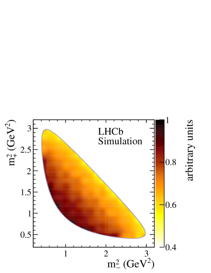
Figure 1: Variation of signal efficiency across the phase space for (left) long and (right) downstream candidates.

5 Analysis strategy and fit results

To determine the $C\!P$ observables $z_{\pm}$ defined in Eq. 6, an unbinned extended maximum likelihood fit is performed in three variables: the ${B}^{0}$ candidate reconstructed invariant mass $m_{{{B}^{0}}}$ and the Dalitz variables $m^{2}_{+}$ and $m^{2}_{-}$. This fit is performed in two steps. First, the signal and background yields and some parameters of the invariant mass PDFs are determined with a fit to the reconstructed ${B}^{0}$ invariant mass distribution, described in Sec. 5.1. An amplitude fit over the phase space of the $D$-meson decay is then performed to measure $z_{\pm}$, using only candidates lying in a $\pm 25\mathrm{\,Me\kern-1.00006ptV}$ window around the fitted ${B}^{0}$ mass, and taking the results of the invariant mass fit as inputs, as explained in Sec. 5.2. The cfit [45] library has been used to perform these fits. Candidate events are divided into four subsamples, according to ${K}^{0}_{\mathrm{\scriptscriptstyle S}}$ type (long or downstream), and whether the candidate is identified as a ${B}^{0}$ or ${\kern 1.79993pt\overline{\kern-1.79993ptB}{}}{}^{0}$-meson decay. In the $B$-candidate invariant mass fit, the ${B}^{0}$ and ${\kern 1.79993pt\overline{\kern-1.79993ptB}{}}{}^{0}$ samples are combined, since identical distributions are expected for this variable, whilst in the $C\!P$ violation observables fit ($C\!P$ fit) they are kept separate.

5.1 Invariant mass fit of ${{B}^{0}}\!\rightarrow{D}{{K}^{*0}}$ candidates

An unbinned extended maximum likelihood fit to the reconstructed invariant mass distributions of the ${B}^{0}$ candidates in the range $[4900,5800]\mathrm{\,Me\kern-1.00006ptV}$ determines the signal and background yields. The long and downstream subsamples are fitted simultaneously. The total PDF includes several components: the ${{B}^{0}}\!\rightarrow{D}{{K}^{*0}}$ signal PDF, background PDFs for ${{B}^{0}_{s}}\!\rightarrow{D}{{\kern 1.99997pt\overline{\kern-1.99997ptK}{}}{}^{*0}}$ decays, combinatorial background, partially reconstructed ${{B}^{0}_{({s})}}\!\rightarrow{{D}^{*}}{\kern 1.79993pt\shortstack{{(\rule[2.15277pt]{12.50002pt}{0.51212pt})} \\ [-.7ex] $\kern-1.79993ptK$}{}{}^{*0}}$ decays and misidentified ${{B}^{0}}\!\rightarrow{D}{{\rho}^{0}}$ decays, as illustrated in Fig. 2.

The fit model is similar to that used in the analysis of ${{B}^{0}}\!\rightarrow{D}{{K}^{*0}}$ decays with $D$-meson decays to two-body final states [25]. The ${{B}^{0}}\!\rightarrow{D}{{K}^{*0}}$ and ${{B}^{0}_{s}}\!\rightarrow{D}{{\kern 1.99997pt\overline{\kern-1.99997ptK}{}}{}^{*0}}$ components are each described as the sum of two Crystal Ball functions [46] sharing the same central value, with the relative yields of the two functions and the tail parameters fixed from simulation. The separation between the central values of the ${{B}^{0}}\!\rightarrow{D}{{K}^{*0}}$ and ${{B}^{0}_{s}}\!\rightarrow{D}{{\kern 1.99997pt\overline{\kern-1.99997ptK}{}}{}^{*0}}$ PDFs is fixed to the known ${B}^{0}$-${B}^{0}_{s}$ mass difference. The ratio of the ${{B}^{0}}\!\rightarrow{D}{{K}^{*0}}$ and ${{B}^{0}_{s}}\!\rightarrow{D}{{\kern 1.99997pt\overline{\kern-1.99997ptK}{}}{}^{*0}}$ yields is constrained to be the same in both the long and downstream subsamples. The combinatorial background is described with an exponential PDF. Partially reconstructed ${{B}^{0}_{({s})}}\!\rightarrow{{D}^{*}}{\kern 1.79993pt\shortstack{{(\rule[2.15277pt]{12.50002pt}{0.51212pt})} \\ [-.7ex] $\kern-1.79993ptK$}{}{}^{*0}}$ decays are described with non-parametric functions obtained by applying kernel density estimation [47] to distributions of simulated events. These distributions depend on the helicity state of the ${D}^{*0}$ meson. Due to parity conservation in ${{D}^{*0}}\!\rightarrow{{D}^{0}}{\gamma}$ and ${{D}^{*0}}\!\rightarrow{{D}^{0}}{{\pi}^{0}}$ decays, two of the three helicity amplitudes have the same invariant mass distribution. The ${{B}^{0}_{s}}\!\rightarrow{{D}^{*}}{{\kern 1.99997pt\overline{\kern-1.99997ptK}{}}{}^{*0}}$ PDF is therefore a linear combination of two non-parametric functions, with the fraction of the longitudinal polarisation in the ${{B}^{0}_{s}}\!\rightarrow{{D}^{*}}{{\kern 1.99997pt\overline{\kern-1.99997ptK}{}}{}^{*0}}$ decays unknown and accounted for with a free parameter in the fit. Each of the two functions describing the different helicity states is a weighted sum of non-parametric functions obtained from simulated ${{B}^{0}_{s}}\!\rightarrow{{D}^{*}}({{D}^{0}}{\gamma}){{\kern 1.99997pt\overline{\kern-1.99997ptK}{}}{}^{*0}}$ and ${{B}^{0}_{s}}\!\rightarrow{{D}^{*}}({{D}^{0}}{{\pi}^{0}}){{\kern 1.99997pt\overline{\kern-1.99997ptK}{}}{}^{*0}}$ decays, taking into account the known ${{D}^{*0}}\!\rightarrow{{D}^{0}}{{\pi}^{0}}$ and ${{D}^{*0}}\!\rightarrow{{D}^{0}}{\gamma}$ branching fractions [48] and the appropriate efficiencies. The PDF for ${{B}^{0}}\!\rightarrow{{D}^{*}}{{K}^{*0}}$ decays is obtained from that for ${{B}^{0}_{s}}\!\rightarrow{{D}^{*}}{{\kern 1.99997pt\overline{\kern-1.99997ptK}{}}{}^{*0}}$ decays, by applying a shift corresponding to the known ${B}^{0}$-${B}^{0}_{s}$ mass difference. In the nominal fit, the polarisation fraction is assumed to be the same for ${{B}^{0}}\!\rightarrow{{D}^{*}}{{K}^{*0}}$ and ${{B}^{0}_{s}}\!\rightarrow{{D}^{*}}{{\kern 1.99997pt\overline{\kern-1.99997ptK}{}}{}^{*0}}$ decays. The effect of this assumption is taken into account in the systematic uncertainties. The ${{B}^{0}}\!\rightarrow{D}{{\rho}^{0}}$ component is also described with a non-parametric function obtained from the simulation, using a data-driven calibration to describe the pion-kaon misidentification efficiency. This component has a very low yield and, to improve the stability of the fit, a Gaussian constraint is applied, requiring the ratio of yields of ${{B}^{0}}\!\rightarrow{D}{{\rho}^{0}}$ and ${{B}^{0}_{s}}\!\rightarrow{D}{{\kern 1.99997pt\overline{\kern-1.99997ptK}{}}{}^{*0}}$ to be consistent with its expected value.

The fitted distribution is shown in Fig 2. The resulting signal and background yields in a $\pm 25\mathrm{\,Me\kern-1.00006ptV}$ range around the ${B}^{0}$ mass are given in Table 1. This range corresponds to the signal region over which the $C\!P$ fit is performed.

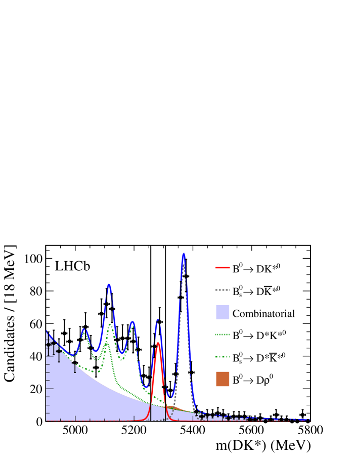
Figure 2: Invariant mass distribution for ${{B}^{0}}\!\rightarrow{D}{{K}^{*0}}$ long and downstream candidates. The fit result, including signal and background components, is superimposed (solid blue). The points are data, and the different fit components are given in the legend. The two vertical lines represent the signal region in which the $C\!P$ fit is performed.

Table 1: Signal and background yields in the signal region, $\pm 25\mathrm{\,Me\kern-1.00006ptV}$ around the ${B}^{0}$ mass, obtained from the invariant mass fit. Total yields, as well as separate yields for long and downstream candidates, are given.

Component	Yield
	Long	Downstream	Total
${{B}^{0}}\!\rightarrow{D}{{K}^{*0}}$	$29\pm 5\phantom{0}$	$60\pm 8\phantom{0}$	$89\pm 11$
${{B}^{0}_{s}}\!\rightarrow{D}{{\kern 1.99997pt\overline{\kern-1.99997ptK}{}}{}^{*0}}$	$0.59\pm 0.12$	$1.21\pm 0.23$	$\phantom{0}1.8\pm 0.3\phantom{0}$
Combinatorial	$\phantom{0}9.6\pm 1.0\phantom{0}$	$16.1\pm 1.4\phantom{0}$	$25.7\pm 1.7\phantom{0}$
${{B}^{0}}\!\rightarrow{{D}^{*}}{{K}^{*0}}$	$0.06\pm 0.02$	$0.06\pm 0.02$	$0.12\pm 0.03$
${{B}^{0}_{s}}\!\rightarrow{{D}^{*}}{{\kern 1.99997pt\overline{\kern-1.99997ptK}{}}{}^{*0}}$	$\phantom{0}4.1\pm 0.8\phantom{0}$	$\phantom{0}7.9\pm 1.3\phantom{0}$	$11.9\pm 1.7\phantom{0}$
${{B}^{0}}\!\rightarrow{D}{{\rho}^{0}}$	$0.20\pm 0.05$	$0.37\pm 0.09$	$0.57\pm 0.11$
Total background	$14.5\pm 1.3\phantom{0}$	$25.6\pm 1.8\phantom{0}$	$40.1\pm 2.4\phantom{0}$

5.2 $C\!P$ fit

A simultaneous unbinned maximum likelihood fit to the four subsamples is performed to determine the $C\!P$ violation observables $z_{\pm}$. The value of the coherence factor is fixed to the central value of ${\kappa}=0.958^{+0.005+0.002}_{-0.010-0.045}$, as measured in the recent LHCb amplitude analysis of ${{B}^{0}}\!\rightarrow{D}{{K}^{+}}{{\pi}^{-}}$ decays [30]. The negative logarithm of the likelihood,

$$\begin{aligned} -\ln\mathcal{L}=&-\sum_{{{B}^{0}}\mathrm{cand.}}\ln\left(\sum_{c}N_{c}f_{c}^{\mathrm{mass}}(m_{B};\vec{q}_{c}^{\ \mathrm{mass}})f_{c}^{{{B}^{0}}\ \mathrm{model}}({m^{2}_{+}},{m^{2}_{-}};{z_{\pm}},\kappa,\vec{q}_{c}^{\ \mathrm{model}})\right)\\ &-\sum_{{{\kern 1.25995pt\overline{\kern-1.25995ptB}{}}{}^{0}}\mathrm{cand.}}\ln\left(\sum_{c}N_{c}f_{c}^{\mathrm{mass}}(m_{B};\vec{q}_{c}^{\ \mathrm{mass}})f_{c}^{{{\kern 1.25995pt\overline{\kern-1.25995ptB}{}}{}^{0}}\ \mathrm{model}}({m^{2}_{+}},{m^{2}_{-}};{z_{\pm}},\kappa,\vec{q}_{c}^{\ \mathrm{model}})\right)\\ &+\sum_{c}N_{c},\end{aligned}$$ (7)

is minimised, where $c$ indexes the different signal and background components, $N_{c}$ is the yield for each category, $f_{c}^{\mathrm{mass}}$ is the invariant mass PDF determined in the previous section, $\vec{q}_{c}^{\mathrm{\ mass}}$ are the mass PDF parameters, $f_{c}^{{B}\ \mathrm{model}}$ is the amplitude PDF and $\vec{q}_{c}^{\mathrm{\ model}}$ are its parameters other than $z_{\pm}$ and $\kappa$, which have been included explicitly.

The non-uniformity of the selection efficiency over the ${D}\!\rightarrow{{K}^{0}_{\mathrm{\scriptscriptstyle S}}}{{\pi}^{+}}{{\pi}^{-}}$ phase space is accounted for by including the function ${\varepsilon}({m^{2}_{+}},{m^{2}_{-}})$, introduced in Sec. 4, within the $f_{c}^{{B}\ \mathrm{model}}$ PDF:

$$f_{c}^{{B}\ \mathrm{model}}({m^{2}_{+}},{m^{2}_{-}};z_{\pm},\kappa,\vec{q}_{c}^{\ \mathrm{model}})=\mathcal{F}_{c}({m^{2}_{+}},{m^{2}_{-}};z_{\pm},\kappa,\vec{q}_{c}^{\ \mathrm{model}})\ {\varepsilon}({m^{2}_{+}},{m^{2}_{-}}),$$ (8)

where $\mathcal{F}_{c}$ is the PDF of the amplitude model.

The model describing the amplitude of the ${D}\!\rightarrow{{K}^{0}_{\mathrm{\scriptscriptstyle S}}}{{\pi}^{+}}{{\pi}^{-}}$ decay over the phase space, $A_{f}\left(m_{+}^{2},m_{-}^{2}\right)$, is identical to that used previously by the BaBar [19, 49] and LHCb [23] collaborations. An isobar model is used to describe $P$-wave (including $\rho(770)^{0}$, $\omega(782)$, Cabibbo-allowed and doubly Cabibbo-suppressed ${{K}^{*}}(892)^{\pm}$ and ${{K}^{*}}(1680)^{-}$) and $D$-wave (including $f_{2}(1270)$ and $K^{*}_{2}(1430)^{\pm}$) contributions. The ${K}\pi$ $S$-wave contribution ($K^{*}_{0}(1430)^{\pm}$) is described using a generalised LASS amplitude [50], whilst the $\pi\pi$ $S$-wave contribution is treated using a $P$-vector approach within the $K$-matrix formalism. All parameters of the model are fixed in the fit to the values determined in Ref. [49].

All components included in the fit of the $B$-meson mass spectrum are included in the fit for the $C\!P$ violation observables, with the exception of the ${{B}^{0}}\!\rightarrow{{D}^{*}}{{K}^{*0}}$ background, because its yield within the signal region is negligible (Table 1). $C\!P$ violation is neglected for ${{B}^{0}_{s}}\!\rightarrow{D}{{\kern 1.99997pt\overline{\kern-1.99997ptK}{}}{}^{*0}}$ and ${{B}^{0}_{s}}\!\rightarrow{{D}^{*}}{{\kern 1.99997pt\overline{\kern-1.99997ptK}{}}{}^{*0}}$ decays, since their Cabbibo-suppressed contributions are negligible. The relevant PDFs are therefore $\mathcal{F}_{{{B}^{0}_{s}}\rightarrow D^{(*)}{{\kern 1.39998pt\overline{\kern-1.39998ptK}{}}{}^{*0}}}=\mathcal{P}(\bar{A}_{f},0,0)$ and $\mathcal{F}_{{{\kern 1.25995pt\overline{\kern-1.25995ptB}{}}{}^{0}_{s}}\rightarrow D^{(*)}{{K}^{*0}}}=\mathcal{P}(A_{f},0,0)$, where $\mathcal{P}$ is defined in Eq. 4. For background arising from misidentified ${{B}^{0}}\!\rightarrow{D}{{\rho}^{0}}$ events, the $B$ flavour state cannot be determined, resulting in an incoherent sum of ${D}^{0}$ and ${\kern 1.99997pt\overline{\kern-1.99997ptD}{}}{}^{0}$ contributions: $\mathcal{F}_{{{B}^{0}}\rightarrow{D}{{\rho}^{0}}}=(|A_{f}|^{2}+|\bar{A}_{f}|^{2})/2$.

The combinatorial background is composed of two contributions: one from non-$D$ candidates, and the other from real $D$ mesons combined with random tracks. Combinatorial $D$ candidates arise from random combinations of four charged tracks, incorrectly reconstructed as a ${D}\!\rightarrow{{K}^{0}_{\mathrm{\scriptscriptstyle S}}}{{\pi}^{+}}{{\pi}^{-}}$ decay, and this contribution is assumed to be distributed uniformly over phase space, $\mathcal{F}_{\mathrm{Comb,\ non-}{D}}=1$, consistent with what is seen in the data. Background from real $D$ candidates arises when the ${{K}^{*}}(892)^{0}$ candidate is reconstructed from random tracks. Consequently, the $B$-meson flavour is unknown, resulting in an incoherent sum, $\mathcal{F}_{\mathrm{Comb,\ real}\ {D}}=(|A_{f}|^{2}+|\bar{A}_{f}|^{2})/2$. The relative proportions of non-$D$ and real $D$ meson backgrounds (${\mathcal{O}}(30\%)$) are fixed using the results of a fit to the reconstructed invariant mass of the $D$ candidates in the signal $B$ mass region. Figures 3 and 4 show the Dalitz plot and its projections, with the fit result superimposed, for ${B}^{0}$ and ${\kern 1.79993pt\overline{\kern-1.79993ptB}{}}{}^{0}$ candidates, respectively. A blinding procedure was used to obscure the values of the $C\!P$ parameters until all aspects of the analysis were finalised. The measured values are

$$x_{-} = -0.15\,\pm 0.14,$$

$$y_{-} = \phantom{-}0.25\,\pm 0.15,$$

$$x_{+} = \phantom{-}0.05\,\pm 0.24,$$

$$y_{+} = -0.65\,^{~{}+0.24}_{~{}-0.23},$$

where the uncertainty is statistical only. The correlation matrix is

$$\begin{matrix}\begin{matrix}\;\;x_{-}\;&\;\;y_{-}\;&\;\;x_{+}\;&\;\;y_{+}\end{matrix}\\ \begin{pmatrix}1&0.14&0&0\\ 0.14&1&0&0\\ 0&0&1&0.14\\ 0&0&0.14&1\\ \end{pmatrix}\\ \end{matrix},$$

and the corresponding likelihood contours for $z_{\pm}$ are shown in Fig. 5.

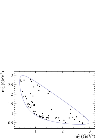
Figure 3: Selected ${{B}^{0}}\!\rightarrow{D}{{K}^{*0}}$ candidates, shown as (a) the Dalitz plot, and its projections on (b) $m^{2}_{-}$, (c) $m^{2}_{+}$ and (d) $m^{2}_{0}$. The line superimposed on the projections corresponds to the fit result and the points are data.

Figure 4: Selected ${{\kern 1.79993pt\overline{\kern-1.79993ptB}{}}{}^{0}}\!\rightarrow{D}{{\kern 1.99997pt\overline{\kern-1.99997ptK}{}}{}^{*0}}$ candidates, shown as (a) the Dalitz plot, and its projections on (b) $m^{2}_{-}$, (c) $m^{2}_{+}$ and (d) $m^{2}_{0}$. The line superimposed on the projections corresponds to the fit result and the points are data.

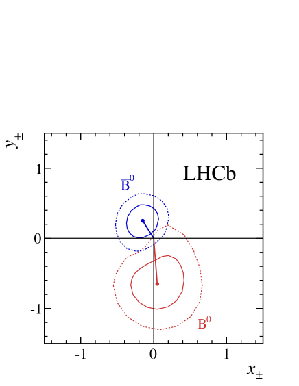
Figure 5: Likelihood contours at 68.3% and 95.5% confidence level for $(x_{+},y_{+})$ (red) and $(x_{-},y_{-})$ (blue), obtained from the $C\!P$ fit.

6 Systematic uncertainties

Several sources of systematic uncertainty on the evaluation of $z_{\pm}$ are considered, and are summarised in Table 2. Unless otherwise stated, for each source considered, the $C\!P$ fit is repeated and the differences in the $z_{\pm}$ values compared to the nominal results are taken as the systematic uncertainties.

Table 2: Summary of the systematic uncertainties on $z_{\pm}$, in units of $(10^{-3})$. The total experimental and total model-related uncertainties are also given as percentages of the statistical uncertainties.

Source of uncertainty	$\delta x_{-}$	$\delta y_{-}$	$\delta x_{+}$	$\delta y_{+}$
Efficiency	5.4	1.1	11	1.8
Invariant mass fit	12	21	15	48
Migration over the phase space	5.3	1.8	6.2	3.0
Misreconstructed signal	7.7	6.6	10	7.1
Background description
Non-$D$ background	20	15	28	47
Real $D$ background	0.1	0.4	0.2	1.0
$C\!P$ violation in ${{B}^{0}_{s}}\!\rightarrow{{D}^{*}}{{\kern 1.99997pt\overline{\kern-1.99997ptK}{}}{}^{*0}}$	1.5	0.8	4.0	1.6
${{B}^{+}}\!\rightarrow{{\kern 1.99997pt\overline{\kern-1.99997ptD}{}}{}^{0}}{{\pi}^{+}}{{\pi}^{+}}{{\pi}^{-}}$ contribution	0.6	1.4	0.8	2.3
${{\mathchar 28931\relax}^{0}_{b}}\!\rightarrow{{D}^{0}}{p}{{\pi}^{-}}$ contribution	0.1	0.7	0.5	1.6
${K}^{*}$ coherence factor ($\kappa$)	4.8	2.4	8.5	2.6
$C\!P$ fit bias	5	49	11	40
Total experimental	26 (19%)	56 (37%)	39 (16%)	78 (33%)
Total model-related (see Table 3)	8 (5%)	7 (5%)	10 (4%)	5 (2%)

The uncertainty on the description of the efficiency variation across the $D$-meson decay phase space arises from several sources. Statistical uncertainties arise due to the limited sizes of the simulated samples used to determine the nominal efficiency function and of the calibration samples used to obtain the data-driven corrections to the PID and hardware trigger efficiencies. Large numbers of alternative efficiency functions are created by smearing these quantities according to their uncertainties. For each fitted $C\!P$ parameter, the residual for a given alternative efficiency function is defined as the difference between its value obtained using this function, and that obtained in the nominal fit. The width of the obtained distribution of residuals is taken as the corresponding systematic uncertainty. Additionally, since the nominal fit is performed using an efficiency function obtained from the simulation applying only BDTA, the fit is repeated using an alternative efficiency function obtained using BDTB, and an uncertainty extracted. The fit is also performed with alternative efficiency functions obtained by varying the fraction of candidates triggered by at least one product of the signal decay chain. Finally, for a few variables used in the BDT, a small difference is observed between the simulation and the background-subtracted data sample. To account for this difference, the simulated events are reweighted to match the data, and the fit is repeated with the resulting efficiency function.

The $B$-meson invariant mass fit result is used to fix the fractions of signal and background and the parameters of the ${B}^{0}$ mass PDF shapes in the $C\!P$ fit. A large number of pseudoexperiments is generated, in which the free parameters of the invariant mass fit are varied within their uncertainties, taking into account their correlations. The $C\!P$ fit is repeated for each variation. For each $C\!P$ parameter, the width from a Gaussian fit to the resulting residual distribution is taken as the associated systematic uncertainty. This is the dominant contribution to the invariant mass fit systematic uncertainty quoted in Table 2. Other uncertainties due to assumptions in the invariant mass fit are evaluated by allowing the ${{B}^{0}}\!\rightarrow{D}{{K}^{*0}}$/${{B}^{0}_{s}}\!\rightarrow{D}{{\kern 1.99997pt\overline{\kern-1.99997ptK}{}}{}^{*0}}$ yield ratio to be different for long and downstream categories, by varying the ${{B}^{0}}\!\rightarrow{D}{{\rho}^{0}}$/${{B}^{0}_{s}}\!\rightarrow{D}{{\kern 1.99997pt\overline{\kern-1.99997ptK}{}}{}^{*0}}$ yield ratio, by varying the Crystal Ball PDF parameters within their uncertainties and by testing alternatives to the Crystal Ball PDFs. The proportions of ${{D}^{*0}}\!\rightarrow{{D}^{0}}{\gamma}$ and ${{D}^{*0}}\!\rightarrow{{D}^{0}}{{\pi}^{0}}$ in the ${{B}^{0}_{({s})}}\!\rightarrow{{D}^{*}}{\kern 1.79993pt\shortstack{{(\rule[2.15277pt]{12.50002pt}{0.51212pt})} \\ [-.7ex] $\kern-1.79993ptK$}{}{}^{*0}}$ background description are also varied, and the effect of neglecting the ${{B}^{0}}\!\rightarrow{{D}^{*}}{{K}^{*0}}$ component in the $C\!P$ fit is evaluated.

The systematic uncertainty due to the finite resolution in ${m^{2}_{\pm}}$ is evaluated with a large number of pseudoexperiments. One nominal pseudodata sample is generated, with $z_{\pm}$ fixed to the values obtained from data. A large number of alternative samples are generated from the nominal one by smearing the ${m^{2}_{\pm}}$ coordinates of each event according to the resolution found in simulation and taking correlations into account. For each $C\!P$ parameter, the width of the residual distribution is taken as the systematic uncertainty.

The misreconstruction of ${{B}^{0}}\!\rightarrow{D}{{K}^{*0}}$ signal events is also studied. This can occur e.g. when the wrong final state pions of a real signal event are combined in the reconstruction of the $D$-meson candidate, leading to migration of this event within the $D$-decay phase space. The uncertainty corresponding to this effect is evaluated using pseudoexperiments. The effect of signal misreconstruction due to ${K}^{*0}$–${\kern 1.99997pt\overline{\kern-1.99997ptK}{}}{}^{*0}$ misidentification, corresponding to a $({{K}^{\pm}}{{\pi}^{\mp}})\rightarrow({{\pi}^{\pm}}{{K}^{\mp}})$ misidentification, is found to be negligible thanks to the PID requirements placed on the ${K}^{*0}$ daughters.

The uncertainty arising from the background description is evaluated for several sources. The $C\!P$ fit is repeated with the fractions of the two categories of combinatorial background (non-$D$ and real $D$ candidates) varied within their uncertainties from the fit to the $D$ invariant mass distribution. Additionally, since in the nominal fit the non-$D$ candidates are assumed to be uniformly distributed over the phase space of the ${D}\!\rightarrow{{K}^{0}_{\mathrm{\scriptscriptstyle S}}}{{\pi}^{+}}{{\pi}^{-}}$ decay, the fit is repeated changing this contribution to the sum of a uniform distribution and a ${{K}^{*}}(892)^{\pm}$ resonance. The relative proportions of the two components are fixed based on the $m^{2}_{\pm}$ distributions found in data. The fit is also repeated with the $D$-meson decay model for the non-$D$ component set to the distribution of data in the $D$ mass sidebands. The uncertainty arising from the poorly-known fraction of non-$D$ and real $D$ background is the dominant systematic uncertainty for the $x_{\pm}$ parameters.

The description of the real $D$ combinatorial background assumes that the probabilities of a ${D}^{0}$ or a ${\kern 1.99997pt\overline{\kern-1.99997ptD}{}}{}^{0}$ being present in an event are equal. The $C\!P$ violation observables fit is repeated with the decay model for this background changed to include a ${D}^{0}$–${\kern 1.99997pt\overline{\kern-1.99997ptD}{}}{}^{0}$ production asymmetry, whose value is set to the measured ${D}^{\pm}$ asymmetry $(-1.0\pm 0.3)\times 10^{-2}$ [51].

$C\!P$ violation is neglected in the ${{B}^{0}_{s}}\!\rightarrow{{D}^{*}}{{\kern 1.99997pt\overline{\kern-1.99997ptK}{}}{}^{*0}}$ decay nominal description. The $C\!P$ fit is repeated with the inclusion of a small component describing the suppressed decay amplitude of ${{B}^{0}_{s}}\!\rightarrow{{D}^{*0}}{{\kern 1.99997pt\overline{\kern-1.99997ptK}{}}{}^{*0}}$, with $C\!P$ violation parameters for this component fixed to ${\gamma}=73.2^{\circ}$, $r_{{{B}^{0}_{s}}}=0.02$ and $\delta_{{{B}^{0}_{s}}}=\{0^{\circ},45^{\circ},90^{\circ},135^{\circ},180^{\circ},225^{\circ},270^{\circ},315^{\circ}\}$. The model used to describe ${{B}^{0}_{s}}\!\rightarrow{{D}^{*}}{{\kern 1.99997pt\overline{\kern-1.99997ptK}{}}{}^{*0}}$ decays consists of an incoherent sum of ${{D}^{*0}}\!\rightarrow{{D}^{0}}{{\pi}^{0}}$ and ${{D}^{*0}}\!\rightarrow{{D}^{0}}{\gamma}$ contributions. Between the ${{D}^{*0}}\!\rightarrow{{D}^{0}}{{\pi}^{0}}$ and ${{D}^{*0}}\!\rightarrow{{D}^{0}}{\gamma}$ decays, there is an effective strong phase shift of $\pi$ that is taken into account [52].

The systematic uncertainties arising from the inclusion of background from misreconstructed ${{B}^{+}}\!\rightarrow{{\kern 1.99997pt\overline{\kern-1.99997ptD}{}}{}^{0}}{{\pi}^{+}}{{\pi}^{+}}{{\pi}^{-}}$ and ${{\mathchar 28931\relax}^{0}_{b}}\!\rightarrow{{D}^{0}}{p}{{\pi}^{-}}$ decays are evaluated, by adding these components into the fit model. The $C\!P$ fit is also repeated with the ${{K}^{*}}(892)^{0}$ coherence factor $\kappa$ varied within its uncertainty [30].

The $C\!P$ fit is verified using one thousand data-sized pseudoexperiments. In each experiment, the signal and background yields, as well as the distributions used in the generation, are fixed to those found in data. The fitted values of $z_{\pm}$ show biases smaller than the statistical uncertainties, and are included as systematic uncertainties. These biases are due to the current limited statistics and are found to reduce in pseudoexperiments generated with a larger sample size.

To evaluate the systematic uncertainty due to the choice of amplitude model for ${D}\!\rightarrow{{K}^{0}_{\mathrm{\scriptscriptstyle S}}}{{\pi}^{+}}{{\pi}^{-}}$, one million ${{B}^{0}}\!\rightarrow{D}{{K}^{*0}}$ and one million ${{B}^{0}_{s}}\!\rightarrow{D}{{\kern 1.99997pt\overline{\kern-1.99997ptK}{}}{}^{*0}}$ decays are simulated according to the nominal decay model, with the Cartesian observables fixed to the nominal fit result. These simulated decays are fitted with alternative models, each of which includes a single modification with respect to the nominal model, as described in the next paragraph. Each of these alternative models is first used to fit the simulated ${{B}^{0}_{s}}\!\rightarrow{D}{{\kern 1.99997pt\overline{\kern-1.99997ptK}{}}{}^{*0}}$ decays to determine values for the resonance coefficients of the model. Those coefficients are then fixed in a second fit, to the simulated ${{B}^{0}}\!\rightarrow{D}{{K}^{*0}}$ decays, to obtain $z_{\pm}$. The systematic uncertainties are taken to be the signed differences in the values of $z_{\pm}$ from the nominal results.

The following changes, labelled (a)-(u), are applied in the alternative models, leading to the uncertainties shown in Table 3:

• $\pi\pi$ S-wave: The $F$-vector model is changed to use two other solutions of the $K$-matrix (from a total of three) determined from fits to scattering data [53] (a), (b). The slowly varying part of the nonresonant term of the $P$-vector is removed (c).

• $K\pi$ S-wave: The generalised LASS parametrisation used to describe the $K^{*}_{0}(1430)^{\pm}$ resonance, is replaced by a relativistic Breit–Wigner propagator with parameters taken from Ref. [54] (d).

• $\pi\pi$ P-wave: The Gounaris–Sakurai propagator is replaced by a relativistic Breit–Wigner propagator [49, 19] (e).

• $K\pi$ P-wave: The mass and width of the ${{K}^{*}}(1680)^{-}$ resonance are varied by their uncertainties from Ref. [50] (f)$-$(i).

• $\pi\pi$ D-wave: The mass and width of the $f_{2}(1270)$ resonance are varied by their uncertainties from Ref. [24] (j)$-$(m).

• $K\pi$ D-wave: The mass and width of the $K^{*}_{2}(1430)^{\pm}$ resonance are varied by their uncertainties from Ref. [55] (n)$-$(q).

• The radius of the Blatt–Weisskopf centrifugal barrier factors, $r_{{\rm BW}}$, is changed from $1.5\,\rm\,GeV^{-1}$ to $0.0\,\rm\,GeV^{-1}$ (r) and $3.0\,\rm\,GeV^{-1}$ (s).

• Two further resonances, ${{K}^{*}}(1410)^{0}$ and $\rho(1450)$, parametrised with relativistic Breit–Wigner propagators, are included in the model [49, 19] (t).

• The Zemach formalism used for the angular distribution of the decay products is replaced by the helicity formalism [49, 19] (u).

It results in total systematic uncertainties arising from the choice of amplitude model of

$$\delta x_{-} =8\times 10^{-3},$$

$$\delta y_{-} =7\times 10^{-3},$$

$$\delta x_{+} =10\times 10^{-3},$$

$$\delta y_{+} =5\times 10^{-3}.$$

Table 3: Model related systematic uncertainties for each alternative model, in units of $(10^{-3})$. The relative signs indicate full correlation or anti-correlation.

	Description		$\delta x_{-}$	$\delta y_{-}$	$\delta x_{+}$	$\delta y_{+}$
(a)	$K$-matrix 1st solution		$-2$	$0.9$	$2$	$1$
(b)	$K$-matrix 2nd solution		$0.3$	$0.3$	$0.0$	$-0.5$
(c)	Remove slowly varying		$-0.7$	$0.2$	$0.5$	$0.6$
	part in $P$-vector
(d)	Generalised LASS		$2$	$3$	$-1$	$3$
	$\rightarrow$ relativistic Breit–Wigner
(e)	Gounaris-Sakurai		$0.7$	$0.0$	$-0.1$	$0.8$
	$\rightarrow$ relativistic Breit–Wigner
(f)	${{K}^{*}}(1680)$	$m+\delta m$	$-0.0$	$0.6$	$0.1$	$0.5$
(g)		$m-\delta m$	$-0.2$	$-0.5$	$0.2$	$-0.9$
(h)		$\Gamma+\delta\Gamma$	$-0.2$	$0.2$	$0.0$	$-0.2$
(i)		$\Gamma-\delta\Gamma$	$0.2$	$-0.1$	$0.5$	$-0.2$
(j)	$f_{2}(1270)$	$m+\delta m$	$-0.1$	$0.0$	$0.3$	$-0.2$
(k)		$m-\delta m$	$-0.0$	$0.1$	$0.2$	$-0.2$
(l)		$\Gamma+\delta\Gamma$	$-0.0$	$0.0$	$0.2$	$-0.2$
(m)		$\Gamma-\delta\Gamma$	$-0.1$	$0.0$	$0.2$	$-0.2$
(n)	$K^{*}_{2}(1430)$	$m+\delta m$	$0.3$	$0.2$	$0.2$	$-0.2$
(o)		$m-\delta m$	$-0.4$	$-0.2$	$0.3$	$-0.1$
(p)		$\Gamma+\delta\Gamma$	$-0.2$	$0.2$	$0.1$	$-0.2$
(q)		$\Gamma-\delta\Gamma$	$0.1$	$-0.1$	$0.3$	$-0.2$
(r)	$r_{{\rm BW}}=0.0\rm\,GeV^{-1}$		$-2$	$0.7$	$-1$	$-0.3$
(s)	$r_{{\rm BW}}=3.0\rm\,GeV^{-1}$		$4$	$-2$	$4$	$2$
(t)	Add ${{K}^{*}}(1410)$ and $\rho(1450)$		$-0.2$	$-0.2$	$0.3$	$-0.3$
(u)	Helicity formalism		$-6$	$6$	$-8$	$2$
	Total model related		$8$	$7$	$10$	$5$

The different systematic uncertainties are combined, assuming that they are independent to obtain the total experimental uncertainties. Depending on the $(x_{\pm},y_{\pm})$ parameters, the leading systematic uncertainties arise from the invariant mass fit, the description of the non-$D$ background and the fit biases. A larger data sample is expected to reduce all three of these uncertainties. Whilst not intrinsically statistical in nature, the systematic uncertainty due to the description of the non-$D$ background is presently evaluated using a conservative approach due to lack of statistics. The total systematic uncertainties, including the model-related uncertainties, are significantly smaller than the statistical uncertainties.

7 Determination of the parameters $\gamma$, $r_{{{B}^{0}}}$ and $\delta_{{{B}^{0}}}$

To determine the physics parameters $r_{{{B}^{0}}}$, $\delta_{{{B}^{0}}}$ and $\gamma$ from the fitted Cartesian observables $z_{\pm}$, the relations

$$\begin{aligned} {x_{\pm}}&={r_{{{B}^{0}}}}\cos({\delta_{{{B}^{0}}}}\pm{\gamma}),\\ {y_{\pm}}&={r_{{{B}^{0}}}}\sin({\delta_{{{B}^{0}}}}\pm{\gamma}),\end{aligned}$$ (9)

must be inverted. This is done using the GammaCombo package, originally developed for the frequentist combination of $\gamma$ measurements by the LHCb collaboration [56, 7]. A global likelihood function is built, which gives the probability of observing a set of $z_{\pm}$ values given the true values $({r_{{{B}^{0}}}},{\delta_{{{B}^{0}}}},\gamma)$,

$$\mathcal{L}({x_{-}},{y_{-}},{x_{+}},{y_{+}}|{r_{{{B}^{0}}}},{\delta_{{{B}^{0}}}},{\gamma}).$$ (10)

All statistical and systematic uncertainties on $z_{\pm}$ are accounted for, as well as the statistical correlation between $z_{\pm}$. Since the precision of the measurement is statistics dominated, correlations between the systematic uncertainties are ignored. Central values for $({r_{{{B}^{0}}}},{\delta_{{{B}^{0}}}},\gamma)$ are obtained by performing a scan of these parameters, to find the values that maximise $\mathcal{L}(x_{-}^{\mathrm{obs}},y_{-}^{\mathrm{obs}},x_{+}^{\mathrm{obs}},y_{+}^{\mathrm{obs}}|{r_{{{B}^{0}}}},{\delta_{{{B}^{0}}}},{\gamma})$, where $z_{\pm}^{\mathrm{obs}}$ are the measured values of the Cartesian observables. Associated confidence intervals may be obtained either from a simple profile-likelihood method, or using the Feldman-Cousins approach [57] combined with a “plugin” method [58]. Confidence level curves for $({r_{{{B}^{0}}}},{\delta_{{{B}^{0}}}},\gamma)$ obtained using the latter method are shown in Figs. 6, 7 and 8. The measured values of $z_{\pm}$ are found to correspond to

$$\gamma =\bigl{(}80^{+21}_{-22}\bigr{)}^{\circ},$$

$${r_{{{B}^{0}}}} =0.39\pm 0.13,$$

$${\delta_{{{B}^{0}}}} =\bigl{(}197^{+24}_{-20}\bigr{)}^{\circ}.$$

Intrinsic to the method used in this analysis [12], there is a two-fold ambiguity in the solution; the Standard Model solution $(0<{\gamma}<180)^{\circ}$ is chosen. Two-dimensional confidence level curves obtained using the profile-likelihood method are shown in Figs. 9 and 10.

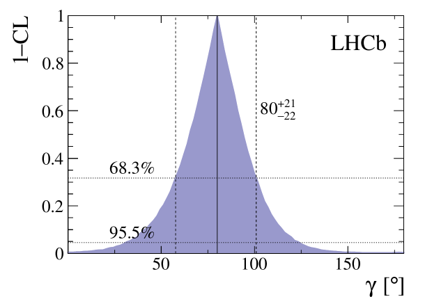
Figure 6: Confidence level curve on $\gamma$, obtained using the “plugin” method [58].

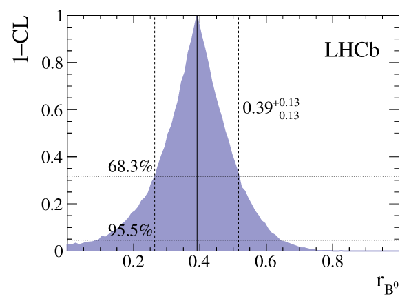
Figure 7: Confidence level curve on $r_{{{B}^{0}}}$, obtained using the “plugin” method [58].

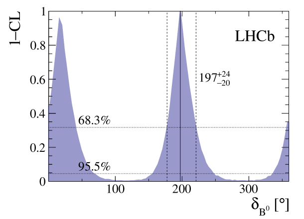
Figure 8: Confidence level curve on $\delta_{{{B}^{0}}}$, obtained using the “plugin” method [58]. Only the $\delta_{{{B}^{0}}}$ solution corresponding to $0<{\gamma}<180^{\circ}$ is highlighted; the other maximum is due to the $({\delta_{{{B}^{0}}}},{\gamma})\rightarrow({\delta_{{{B}^{0}}}}+\pi,{\gamma}+\pi)$ ambiguity.

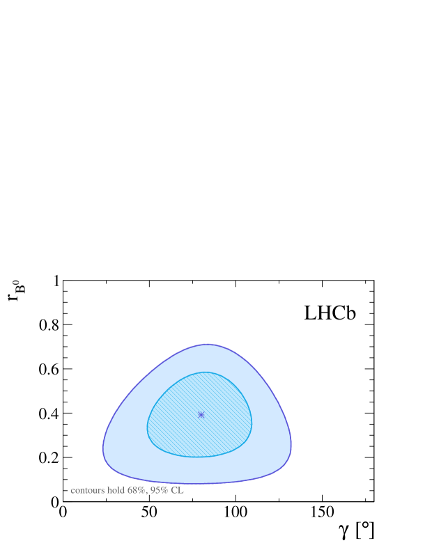
Figure 9: Two-dimensional confidence level curves in the $({\gamma},{r_{{{B}^{0}}}})$ plane, obtained using the profile-likelihood method.

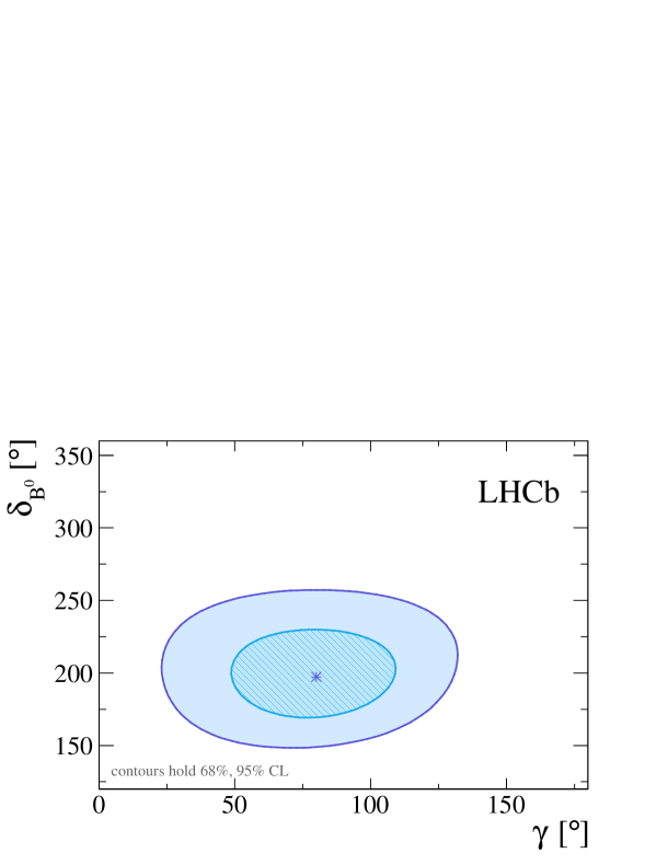
Figure 10: Two-dimensional confidence level curves in the $({\gamma},{\delta_{{{B}^{0}}}})$ plane, obtained using the profile-likelihood method.

8 Conclusion

An amplitude analysis of ${{B}^{0}}\!\rightarrow{D}{{K}^{*0}}$ decays, employing a model description of the ${D}\!\rightarrow{{K}^{0}_{\mathrm{\scriptscriptstyle S}}}{{\pi}^{+}}{{\pi}^{-}}$ decay, has been performed using data corresponding to an integrated luminosity of $3\mbox{\,fb}^{-1}$, recorded by LHCb at a centre-of-mass energy of $7\mathrm{\,Te\kern-1.00006ptV}$ in 2011 and $8\mathrm{\,Te\kern-1.00006ptV}$ in 2012. The measured values of the $C\!P$ violation observables ${x_{\pm}}={r_{{{B}^{0}}}}\cos{({\delta_{{{B}^{0}}}}\pm{\gamma})}$ and ${y_{\pm}}={r_{{{B}^{0}}}}\sin{({\delta_{{{B}^{0}}}}\pm{\gamma})}$ are

$$x_{-} = -0.15\,\pm 0.14\pm 0.03\pm 0.01,$$

$$y_{-} = \phantom{-}0.25\,\pm 0.15\pm 0.06\pm 0.01,$$

$$x_{+} = \phantom{-}0.05\,\pm 0.24\pm 0.04\pm 0.01,$$

$$y_{+} = -0.65~{}^{+0.24~{}~{}~{}}_{-0.23~{}~{}~{}}\pm 0.08\pm 0.01,$$

where the first uncertainties are statistical, the second are systematic and the third are due to the choice of amplitude model used to describe the ${D}\!\rightarrow{{K}^{0}_{\mathrm{\scriptscriptstyle S}}}{{\pi}^{+}}{{\pi}^{-}}$ decay. These are the most precise measurements of these observables related to the neutral channel ${{B}^{0}}\!\rightarrow{D}{{K}^{*0}}$. They place constraints on the magnitude of the ratio of the interfering $B$-meson decay amplitudes, the strong phase difference between them and the CKM angle $\gamma$, giving the values

$$\gamma = \bigl{(}80^{+21}_{-22}\bigr{)}^{\circ},$$

$${r_{{{B}^{0}}}} = 0.39\pm 0.13,$$

$${\delta_{{{B}^{0}}}} = \bigl{(}197^{+24}_{-20}\bigr{)}^{\circ}.$$

Here, $r_{{{B}^{0}}}$ and $\delta_{{{B}^{0}}}$ are defined for a $K\pi$ mass region of $\pm 50{\mathrm{\,Me\kern-1.00006ptV\!}}$ around the ${{K}^{*}}(892)^{0}$ mass and for an absolute value of the cosine of the ${K}^{*0}$ decay angle greater than $0.4$. These results are consistent with, and have lower total uncertainties than those reported in Ref. [28], where a model independent analysis method is used. The two results are based on the same data set and cannot be combined. The consistency shows that at the current level of statistical precision the assumptions used to obtain the present result are justified.

LHCb collaboration

R. Aaij³⁹, C. Abellán Beteta⁴¹, B. Adeva³⁸, M. Adinolfi⁴⁷, Z. Ajaltouni⁵, S. Akar⁶, J. Albrecht¹⁰, F. Alessio³⁹, M. Alexander⁵², S. Ali⁴², G. Alkhazov³¹, P. Alvarez Cartelle⁵⁴, A.A. Alves Jr⁵⁸, S. Amato², S. Amerio²³, Y. Amhis⁷, L. An⁴⁰, L. Anderlini¹⁸, G. Andreassi⁴⁰, M. Andreotti^17,g, J.E. Andrews⁵⁹, R.B. Appleby⁵⁵, O. Aquines Gutierrez¹¹, F. Archilli³⁹, P. d’Argent¹², A. Artamonov³⁶, M. Artuso⁶⁰, E. Aslanides⁶, G. Auriemma^26,s, M. Baalouch⁵, S. Bachmann¹², J.J. Back⁴⁹, A. Badalov³⁷, C. Baesso⁶¹, W. Baldini¹⁷, R.J. Barlow⁵⁵, C. Barschel³⁹, S. Barsuk⁷, W. Barter³⁹, V. Batozskaya²⁹, V. Battista⁴⁰, A. Bay⁴⁰, L. Beaucourt⁴, J. Beddow⁵², F. Bedeschi²⁴, I. Bediaga¹, L.J. Bel⁴², V. Bellee⁴⁰, N. Belloli^21,i, I. Belyaev³², E. Ben-Haim⁸, G. Bencivenni¹⁹, S. Benson³⁹, J. Benton⁴⁷, A. Berezhnoy³³, R. Bernet⁴¹, A. Bertolin²³, M.-O. Bettler³⁹, M. van Beuzekom⁴², S. Bifani⁴⁶, P. Billoir⁸, T. Bird⁵⁵, A. Birnkraut¹⁰, A. Bitadze⁵⁵, A. Bizzeti^18,u, T. Blake⁴⁹, F. Blanc⁴⁰, J. Blouw¹¹, S. Blusk⁶⁰, V. Bocci²⁶, A. Bondar³⁵, N. Bondar^31,39, W. Bonivento¹⁶, S. Borghi⁵⁵, M. Borsato³⁸, M. Boubdir⁹, T.J.V. Bowcock⁵³, E. Bowen⁴¹, C. Bozzi^17,39, S. Braun¹², M. Britsch¹², T. Britton⁶⁰, J. Brodzicka⁵⁵, E. Buchanan⁴⁷, C. Burr⁵⁵, A. Bursche², J. Buytaert³⁹, S. Cadeddu¹⁶, R. Calabrese^17,g, M. Calvi^21,i, M. Calvo Gomez^37,m, P. Campana¹⁹, D. Campora Perez³⁹, L. Capriotti⁵⁵, A. Carbone^15,e, G. Carboni^25,j, R. Cardinale^20,h, A. Cardini¹⁶, P. Carniti^21,i, L. Carson⁵¹, K. Carvalho Akiba², G. Casse⁵³, L. Cassina^21,i, L. Castillo Garcia⁴⁰, M. Cattaneo³⁹, Ch. Cauet¹⁰, G. Cavallero²⁰, R. Cenci^24,t, M. Charles⁸, Ph. Charpentier³⁹, M. Chefdeville⁴, S. Chen⁵⁵, S.-F. Cheung⁵⁶, V. Chobanova³⁸, M. Chrzaszcz^41,27, X. Cid Vidal³⁹, G. Ciezarek⁴², P.E.L. Clarke⁵¹, M. Clemencic³⁹, H.V. Cliff⁴⁸, J. Closier³⁹, V. Coco⁵⁸, J. Cogan⁶, E. Cogneras⁵, V. Cogoni^16,f, L. Cojocariu³⁰, G. Collazuol^23,o, P. Collins³⁹, A. Comerma-Montells¹², A. Contu³⁹, A. Cook⁴⁷, S. Coquereau⁸, G. Corti³⁹, M. Corvo^17,g, B. Couturier³⁹, G.A. Cowan⁵¹, D.C. Craik⁵¹, A. Crocombe⁴⁹, M. Cruz Torres⁶¹, S. Cunliffe⁵⁴, R. Currie⁵⁴, C. D’Ambrosio³⁹, E. Dall’Occo⁴², J. Dalseno⁴⁷, P.N.Y. David⁴², A. Davis⁵⁸, O. De Aguiar Francisco², K. De Bruyn⁶, S. De Capua⁵⁵, M. De Cian¹², J.M. De Miranda¹, L. De Paula², P. De Simone¹⁹, C.-T. Dean⁵², D. Decamp⁴, M. Deckenhoff¹⁰, L. Del Buono⁸, M. Demmer¹⁰, D. Derkach⁶⁷, O. Deschamps⁵, F. Dettori³⁹, B. Dey²², A. Di Canto³⁹, H. Dijkstra³⁹, F. Dordei³⁹, M. Dorigo⁴⁰, A. Dosil Suárez³⁸, A. Dovbnya⁴⁴, K. Dreimanis⁵³, L. Dufour⁴², G. Dujany⁵⁵, P. Durante³⁹, R. Dzhelyadin³⁶, A. Dziurda³⁹, A. Dzyuba³¹, N. Déléage⁴, S. Easo^50,39, U. Egede⁵⁴, V. Egorychev³², S. Eidelman³⁵, S. Eisenhardt⁵¹, U. Eitschberger¹⁰, R. Ekelhof¹⁰, L. Eklund⁵², I. El Rifai⁵, Ch. Elsasser⁴¹, S. Ely⁶⁰, S. Esen¹², H.M. Evans⁴⁸, T. Evans⁵⁶, A. Falabella¹⁵, N. Farley⁴⁶, S. Farry⁵³, R. Fay⁵³, D. Ferguson⁵¹, V. Fernandez Albor³⁸, F. Ferrari^15,39, F. Ferreira Rodrigues¹, M. Ferro-Luzzi³⁹, S. Filippov³⁴, M. Fiore^17,g, M. Fiorini^17,g, M. Firlej²⁸, C. Fitzpatrick⁴⁰, T. Fiutowski²⁸, F. Fleuret^7,b, K. Fohl³⁹, M. Fontana¹⁶, F. Fontanelli^20,h, D.C. Forshaw⁶⁰, R. Forty³⁹, M. Frank³⁹, C. Frei³⁹, M. Frosini¹⁸, J. Fu²², E. Furfaro^25,j, C. Färber³⁹, A. Gallas Torreira³⁸, D. Galli^15,e, S. Gallorini²³, S. Gambetta⁵¹, M. Gandelman², P. Gandini⁵⁶, Y. Gao³, J. García Pardiñas³⁸, J. Garra Tico⁴⁸, L. Garrido³⁷, P.J. Garsed⁴⁸, D. Gascon³⁷, C. Gaspar³⁹, L. Gavardi¹⁰, G. Gazzoni⁵, D. Gerick¹², E. Gersabeck¹², M. Gersabeck⁵⁵, T. Gershon⁴⁹, Ph. Ghez⁴, S. Gianì⁴⁰, V. Gibson⁴⁸, O.G. Girard⁴⁰, L. Giubega³⁰, V.V. Gligorov⁸, D. Golubkov³², A. Golutvin^54,39, A. Gomes^1,a, C. Gotti^21,i, M. Grabalosa Gándara⁵, R. Graciani Diaz³⁷, L.A. Granado Cardoso³⁹, E. Graugés³⁷, E. Graverini⁴¹, G. Graziani¹⁸, A. Grecu³⁰, P. Griffith⁴⁶, L. Grillo¹², O. Grünberg⁶⁵, E. Gushchin³⁴, Yu. Guz^36,39, T. Gys³⁹, C. Göbel⁶¹, T. Hadavizadeh⁵⁶, C. Hadjivasiliou⁶⁰, G. Haefeli⁴⁰, C. Haen³⁹, S.C. Haines⁴⁸, S. Hall⁵⁴, B. Hamilton⁵⁹, X. Han¹², S. Hansmann-Menzemer¹², N. Harnew⁵⁶, S.T. Harnew⁴⁷, J. Harrison⁵⁵, J. He³⁹, T. Head⁴⁰, A. Heister⁹, K. Hennessy⁵³, P. Henrard⁵, L. Henry⁸, J.A. Hernando Morata³⁸, E. van Herwijnen³⁹, M. Heß⁶⁵, A. Hicheur², D. Hill⁵⁶, M. Hoballah⁵, C. Hombach⁵⁵, W. Hulsbergen⁴², T. Humair⁵⁴, N. Hussain⁵⁶, D. Hutchcroft⁵³, M. Idzik²⁸, P. Ilten⁵⁷, R. Jacobsson³⁹, A. Jaeger¹², J. Jalocha⁵⁶, E. Jans⁴², A. Jawahery⁵⁹, M. John⁵⁶, D. Johnson³⁹, C.R. Jones⁴⁸, C. Joram³⁹, B. Jost³⁹, N. Jurik⁶⁰, S. Kandybei⁴⁴, W. Kanso⁶, M. Karacson³⁹, T.M. Karbach^39,†, S. Karodia⁵², M. Kecke¹², M. Kelsey⁶⁰, I.R. Kenyon⁴⁶, M. Kenzie³⁹, T. Ketel⁴³, E. Khairullin⁶⁷, B. Khanji^21,39,i, C. Khurewathanakul⁴⁰, T. Kirn⁹, S. Klaver⁵⁵, K. Klimaszewski²⁹, M. Kolpin¹², I. Komarov⁴⁰, R.F. Koopman⁴³, P. Koppenburg⁴², M. Kozeiha⁵, L. Kravchuk³⁴, K. Kreplin¹², M. Kreps⁴⁹, P. Krokovny³⁵, F. Kruse¹⁰, W. Krzemien²⁹, W. Kucewicz^27,l, M. Kucharczyk²⁷, V. Kudryavtsev³⁵, A.K. Kuonen⁴⁰, K. Kurek²⁹, T. Kvaratskheliya³², D. Lacarrere³⁹, G. Lafferty^55,39, A. Lai¹⁶, D. Lambert⁵¹, G. Lanfranchi¹⁹, C. Langenbruch⁴⁹, B. Langhans³⁹, T. Latham⁴⁹, C. Lazzeroni⁴⁶, R. Le Gac⁶, J. van Leerdam⁴², J.-P. Lees⁴, A. Leflat^33,39, J. Lefrançois⁷, R. Lefèvre⁵, E. Lemos Cid³⁸, O. Leroy⁶, T. Lesiak²⁷, B. Leverington¹², Y. Li⁷, T. Likhomanenko^67,66, R. Lindner³⁹, C. Linn³⁹, F. Lionetto⁴¹, B. Liu¹⁶, X. Liu³, D. Loh⁴⁹, I. Longstaff⁵², J.H. Lopes², D. Lucchesi^23,o, M. Lucio Martinez³⁸, H. Luo⁵¹, A. Lupato²³, E. Luppi^17,g, O. Lupton⁵⁶, A. Lusiani²⁴, X. Lyu⁶², F. Machefert⁷, F. Maciuc³⁰, O. Maev³¹, K. Maguire⁵⁵, S. Malde⁵⁶, A. Malinin⁶⁶, G. Manca⁷, G. Mancinelli⁶, P. Manning⁶⁰, A. Mapelli³⁹, J. Maratas⁵, J.F. Marchand⁴, U. Marconi¹⁵, C. Marin Benito³⁷, P. Marino^24,t, J. Marks¹², G. Martellotti²⁶, M. Martin⁶, M. Martinelli⁴⁰, D. Martinez Santos³⁸, F. Martinez Vidal⁶⁸, D. Martins Tostes², L.M. Massacrier⁷, A. Massafferri¹, R. Matev³⁹, A. Mathad⁴⁹, Z. Mathe³⁹, C. Matteuzzi²¹, A. Mauri⁴¹, B. Maurin⁴⁰, A. Mazurov⁴⁶, M. McCann⁵⁴, J. McCarthy⁴⁶, A. McNab⁵⁵, R. McNulty¹³, B. Meadows⁵⁸, F. Meier¹⁰, M. Meissner¹², D. Melnychuk²⁹, M. Merk⁴², E Michielin²³, D.A. Milanes⁶⁴, M.-N. Minard⁴, D.S. Mitzel¹², J. Molina Rodriguez⁶¹, I.A. Monroy⁶⁴, S. Monteil⁵, M. Morandin²³, P. Morawski²⁸, A. Mordà⁶, M.J. Morello^24,t, J. Moron²⁸, A.B. Morris⁵¹, R. Mountain⁶⁰, F. Muheim⁵¹, M. Mussini¹⁵, B. Muster⁴⁰, D. Müller⁵⁵, J. Müller¹⁰, K. Müller⁴¹, V. Müller¹⁰, P. Naik⁴⁷, T. Nakada⁴⁰, R. Nandakumar⁵⁰, A. Nandi⁵⁶, I. Nasteva², M. Needham⁵¹, N. Neri²², S. Neubert¹², N. Neufeld³⁹, M. Neuner¹², A.D. Nguyen⁴⁰, C. Nguyen-Mau^40,n, V. Niess⁵, S. Nieswand⁹, R. Niet¹⁰, N. Nikitin³³, T. Nikodem¹², A. Novoselov³⁶, D.P. O’Hanlon⁴⁹, A. Oblakowska-Mucha²⁸, V. Obraztsov³⁶, S. Ogilvy¹⁹, O. Okhrimenko⁴⁵, R. Oldeman⁴⁸, C.J.G. Onderwater⁶⁹, B. Osorio Rodrigues¹, J.M. Otalora Goicochea², A. Otto³⁹, P. Owen⁵⁴, A. Oyanguren⁶⁸, A. Palano^14,d, F. Palombo^22,q, M. Palutan¹⁹, J. Panman³⁹, A. Papanestis⁵⁰, M. Pappagallo⁵², L.L. Pappalardo^17,g, C. Pappenheimer⁵⁸, W. Parker⁵⁹, C. Parkes⁵⁵, G. Passaleva¹⁸, G.D. Patel⁵³, M. Patel⁵⁴, C. Patrignani^15,e, A. Pearce^55,50, A. Pellegrino⁴², G. Penso^26,k, M. Pepe Altarelli³⁹, S. Perazzini³⁹, P. Perret⁵, L. Pescatore⁴⁶, K. Petridis⁴⁷, A. Petrolini^20,h, M. Petruzzo²², E. Picatoste Olloqui³⁷, B. Pietrzyk⁴, D. Pinci²⁶, A. Pistone²⁰, A. Piucci¹², S. Playfer⁵¹, M. Plo Casasus³⁸, T. Poikela³⁹, F. Polci⁸, A. Poluektov^49,35, I. Polyakov³², E. Polycarpo², A. Popov³⁶, D. Popov^11,39, B. Popovici³⁰, C. Potterat², E. Price⁴⁷, J.D. Price⁵³, J. Prisciandaro³⁸, A. Pritchard⁵³, C. Prouve⁴⁷, V. Pugatch⁴⁵, A. Puig Navarro⁴⁰, G. Punzi^24,p, W. Qian⁵⁶, R. Quagliani^7,47, B. Rachwal²⁷, J.H. Rademacker⁴⁷, M. Rama²⁴, M. Ramos Pernas³⁸, M.S. Rangel², I. Raniuk⁴⁴, G. Raven⁴³, F. Redi⁵⁴, S. Reichert¹⁰, A.C. dos Reis¹, V. Renaudin⁷, S. Ricciardi⁵⁰, S. Richards⁴⁷, M. Rihl³⁹, K. Rinnert^53,39, V. Rives Molina³⁷, P. Robbe⁷, A.B. Rodrigues¹, E. Rodrigues⁵⁵, J.A. Rodriguez Lopez⁶⁴, P. Rodriguez Perez⁵⁵, A. Rogozhnikov⁶⁷, S. Roiser³⁹, V. Romanovskiy³⁶, A. Romero Vidal³⁸, J.W. Ronayne¹³, M. Rotondo²³, T. Ruf³⁹, P. Ruiz Valls⁶⁸, J.J. Saborido Silva³⁸, N. Sagidova³¹, B. Saitta^16,f, V. Salustino Guimaraes², C. Sanchez Mayordomo⁶⁸, B. Sanmartin Sedes³⁸, R. Santacesaria²⁶, C. Santamarina Rios³⁸, M. Santimaria¹⁹, E. Santovetti^25,j, A. Sarti^19,k, C. Satriano^26,s, A. Satta²⁵, D.M. Saunders⁴⁷, D. Savrina^32,33, S. Schael⁹, M. Schiller³⁹, H. Schindler³⁹, M. Schlupp¹⁰, M. Schmelling¹¹, T. Schmelzer¹⁰, B. Schmidt³⁹, O. Schneider⁴⁰, A. Schopper³⁹, M. Schubiger⁴⁰, M.-H. Schune⁷, R. Schwemmer³⁹, B. Sciascia¹⁹, A. Sciubba^26,k, A. Semennikov³², A. Sergi⁴⁶, N. Serra⁴¹, J. Serrano⁶, L. Sestini²³, P. Seyfert²¹, M. Shapkin³⁶, I. Shapoval^17,44,g, Y. Shcheglov³¹, T. Shears⁵³, L. Shekhtman³⁵, V. Shevchenko⁶⁶, A. Shires¹⁰, B.G. Siddi¹⁷, R. Silva Coutinho⁴¹, L. Silva de Oliveira², G. Simi^23,o, M. Sirendi⁴⁸, N. Skidmore⁴⁷, T. Skwarnicki⁶⁰, E. Smith⁵⁴, I.T. Smith⁵¹, J. Smith⁴⁸, M. Smith⁵⁵, H. Snoek⁴², M.D. Sokoloff⁵⁸, F.J.P. Soler⁵², F. Soomro⁴⁰, D. Souza⁴⁷, B. Souza De Paula², B. Spaan¹⁰, P. Spradlin⁵², S. Sridharan³⁹, F. Stagni³⁹, M. Stahl¹², S. Stahl³⁹, S. Stefkova⁵⁴, O. Steinkamp⁴¹, O. Stenyakin³⁶, S. Stevenson⁵⁶, S. Stoica³⁰, S. Stone⁶⁰, B. Storaci⁴¹, S. Stracka^24,t, M. Straticiuc³⁰, U. Straumann⁴¹, L. Sun⁵⁸, W. Sutcliffe⁵⁴, K. Swientek²⁸, S. Swientek¹⁰, V. Syropoulos⁴³, M. Szczekowski²⁹, T. Szumlak²⁸, S. T’Jampens⁴, A. Tayduganov⁶, T. Tekampe¹⁰, G. Tellarini^17,g, F. Teubert³⁹, C. Thomas⁵⁶, E. Thomas³⁹, J. van Tilburg⁴², V. Tisserand⁴, M. Tobin⁴⁰, S. Tolk⁴³, L. Tomassetti^17,g, D. Tonelli³⁹, S. Topp-Joergensen⁵⁶, E. Tournefier⁴, S. Tourneur⁴⁰, K. Trabelsi⁴⁰, M.T. Tran⁴⁰, M. Tresch⁴¹, A. Trisovic³⁹, A. Tsaregorodtsev⁶, P. Tsopelas⁴², N. Tuning^42,39, A. Ukleja²⁹, A. Ustyuzhanin^67,66, U. Uwer¹², C. Vacca^16,39,f, V. Vagnoni^15,39, S. Valat³⁹, G. Valenti¹⁵, A. Vallier⁷, R. Vazquez Gomez¹⁹, P. Vazquez Regueiro³⁸, S. Vecchi¹⁷, M. van Veghel⁴², J.J. Velthuis⁴⁷, M. Veltri^18,r, G. Veneziano⁴⁰, M. Vesterinen¹², B. Viaud⁷, D.  Vieira², M. Vieites Diaz³⁸, X. Vilasis-Cardona^37,m, V. Volkov³³, A. Vollhardt⁴¹, D. Voong⁴⁷, A. Vorobyev³¹, V. Vorobyev³⁵, C. Voß⁶⁵, J.A. de Vries⁴², C. Vázquez Sierra³⁸, R. Waldi⁶⁵, C. Wallace⁴⁹, R. Wallace¹³, J. Walsh²⁴, J. Wang⁶⁰, D.R. Ward⁴⁸, N.K. Watson⁴⁶, D. Websdale⁵⁴, A. Weiden⁴¹, M. Whitehead³⁹, J. Wicht⁴⁹, G. Wilkinson^56,39, M. Wilkinson⁶⁰, M. Williams³⁹, M.P. Williams⁴⁶, M. Williams⁵⁷, T. Williams⁴⁶, F.F. Wilson⁵⁰, J. Wimberley⁵⁹, J. Wishahi¹⁰, W. Wislicki²⁹, M. Witek²⁷, G. Wormser⁷, S.A. Wotton⁴⁸, K. Wraight⁵², S. Wright⁴⁸, K. Wyllie³⁹, Y. Xie⁶³, Z. Xu⁴⁰, Z. Yang³, H. Yin⁶³, J. Yu⁶³, X. Yuan³⁵, O. Yushchenko³⁶, M. Zangoli¹⁵, M. Zavertyaev^11,c, L. Zhang³, Y. Zhang⁷, A. Zhelezov¹², Y. Zheng⁶², A. Zhokhov³², L. Zhong³, V. Zhukov⁹, S. Zucchelli¹⁵.

¹Centro Brasileiro de Pesquisas Físicas (CBPF), Rio de Janeiro, Brazil
²Universidade Federal do Rio de Janeiro (UFRJ), Rio de Janeiro, Brazil
³Center for High Energy Physics, Tsinghua University, Beijing, China
⁴LAPP, Université Savoie Mont-Blanc, CNRS/IN2P3, Annecy-Le-Vieux, France
⁵Clermont Université, Université Blaise Pascal, CNRS/IN2P3, LPC, Clermont-Ferrand, France
⁶CPPM, Aix-Marseille Université, CNRS/IN2P3, Marseille, France
⁷LAL, Université Paris-Sud, CNRS/IN2P3, Orsay, France
⁸LPNHE, Université Pierre et Marie Curie, Université Paris Diderot, CNRS/IN2P3, Paris, France
⁹I. Physikalisches Institut, RWTH Aachen University, Aachen, Germany
¹⁰Fakultät Physik, Technische Universität Dortmund, Dortmund, Germany
¹¹Max-Planck-Institut für Kernphysik (MPIK), Heidelberg, Germany
¹²Physikalisches Institut, Ruprecht-Karls-Universität Heidelberg, Heidelberg, Germany
¹³School of Physics, University College Dublin, Dublin, Ireland
¹⁴Sezione INFN di Bari, Bari, Italy
¹⁵Sezione INFN di Bologna, Bologna, Italy
¹⁶Sezione INFN di Cagliari, Cagliari, Italy
¹⁷Sezione INFN di Ferrara, Ferrara, Italy
¹⁸Sezione INFN di Firenze, Firenze, Italy
¹⁹Laboratori Nazionali dell’INFN di Frascati, Frascati, Italy
²⁰Sezione INFN di Genova, Genova, Italy
²¹Sezione INFN di Milano Bicocca, Milano, Italy
²²Sezione INFN di Milano, Milano, Italy
²³Sezione INFN di Padova, Padova, Italy
²⁴Sezione INFN di Pisa, Pisa, Italy
²⁵Sezione INFN di Roma Tor Vergata, Roma, Italy
²⁶Sezione INFN di Roma La Sapienza, Roma, Italy
²⁷Henryk Niewodniczanski Institute of Nuclear Physics Polish Academy of Sciences, Kraków, Poland
²⁸AGH - University of Science and Technology, Faculty of Physics and Applied Computer Science, Kraków, Poland
²⁹National Center for Nuclear Research (NCBJ), Warsaw, Poland
³⁰Horia Hulubei National Institute of Physics and Nuclear Engineering, Bucharest-Magurele, Romania
³¹Petersburg Nuclear Physics Institute (PNPI), Gatchina, Russia
³²Institute of Theoretical and Experimental Physics (ITEP), Moscow, Russia
³³Institute of Nuclear Physics, Moscow State University (SINP MSU), Moscow, Russia
³⁴Institute for Nuclear Research of the Russian Academy of Sciences (INR RAN), Moscow, Russia
³⁵Budker Institute of Nuclear Physics (SB RAS) and Novosibirsk State University, Novosibirsk, Russia
³⁶Institute for High Energy Physics (IHEP), Protvino, Russia
³⁷Universitat de Barcelona, Barcelona, Spain
³⁸Universidad de Santiago de Compostela, Santiago de Compostela, Spain
³⁹European Organization for Nuclear Research (CERN), Geneva, Switzerland
⁴⁰Ecole Polytechnique Fédérale de Lausanne (EPFL), Lausanne, Switzerland
⁴¹Physik-Institut, Universität Zürich, Zürich, Switzerland
⁴²Nikhef National Institute for Subatomic Physics, Amsterdam, The Netherlands
⁴³Nikhef National Institute for Subatomic Physics and VU University Amsterdam, Amsterdam, The Netherlands
⁴⁴NSC Kharkiv Institute of Physics and Technology (NSC KIPT), Kharkiv, Ukraine
⁴⁵Institute for Nuclear Research of the National Academy of Sciences (KINR), Kyiv, Ukraine
⁴⁶University of Birmingham, Birmingham, United Kingdom
⁴⁷H.H. Wills Physics Laboratory, University of Bristol, Bristol, United Kingdom
⁴⁸Cavendish Laboratory, University of Cambridge, Cambridge, United Kingdom
⁴⁹Department of Physics, University of Warwick, Coventry, United Kingdom
⁵⁰STFC Rutherford Appleton Laboratory, Didcot, United Kingdom
⁵¹School of Physics and Astronomy, University of Edinburgh, Edinburgh, United Kingdom
⁵²School of Physics and Astronomy, University of Glasgow, Glasgow, United Kingdom
⁵³Oliver Lodge Laboratory, University of Liverpool, Liverpool, United Kingdom
⁵⁴Imperial College London, London, United Kingdom
⁵⁵School of Physics and Astronomy, University of Manchester, Manchester, United Kingdom
⁵⁶Department of Physics, University of Oxford, Oxford, United Kingdom
⁵⁷Massachusetts Institute of Technology, Cambridge, MA, United States
⁵⁸University of Cincinnati, Cincinnati, OH, United States
⁵⁹University of Maryland, College Park, MD, United States
⁶⁰Syracuse University, Syracuse, NY, United States
⁶¹Pontifícia Universidade Católica do Rio de Janeiro (PUC-Rio), Rio de Janeiro, Brazil, associated to ^2
62University of Chinese Academy of Sciences, Beijing, China, associated to ^3
63Institute of Particle Physics, Central China Normal University, Wuhan, Hubei, China, associated to ^3
64Departamento de Fisica , Universidad Nacional de Colombia, Bogota, Colombia, associated to ^8
65Institut für Physik, Universität Rostock, Rostock, Germany, associated to ^12
66National Research Centre Kurchatov Institute, Moscow, Russia, associated to ^32
67Yandex School of Data Analysis, Moscow, Russia, associated to ^32
68Instituto de Fisica Corpuscular (IFIC), Universitat de Valencia-CSIC, Valencia, Spain, associated to ^37
69Van Swinderen Institute, University of Groningen, Groningen, The Netherlands, associated to <sup>42

a</sup>Universidade Federal do Triângulo Mineiro (UFTM), Uberaba-MG, Brazil
^bLaboratoire Leprince-Ringuet, Palaiseau, France
^cP.N. Lebedev Physical Institute, Russian Academy of Science (LPI RAS), Moscow, Russia
^dUniversità di Bari, Bari, Italy
^eUniversità di Bologna, Bologna, Italy
^fUniversità di Cagliari, Cagliari, Italy
^gUniversità di Ferrara, Ferrara, Italy
^hUniversità di Genova, Genova, Italy
ⁱUniversità di Milano Bicocca, Milano, Italy
^jUniversità di Roma Tor Vergata, Roma, Italy
^kUniversità di Roma La Sapienza, Roma, Italy
^lAGH - University of Science and Technology, Faculty of Computer Science, Electronics and Telecommunications, Kraków, Poland
^mLIFAELS, La Salle, Universitat Ramon Llull, Barcelona, Spain
ⁿHanoi University of Science, Hanoi, Viet Nam
^oUniversità di Padova, Padova, Italy
^pUniversità di Pisa, Pisa, Italy
^qUniversità degli Studi di Milano, Milano, Italy
^rUniversità di Urbino, Urbino, Italy
^sUniversità della Basilicata, Potenza, Italy
^tScuola Normale Superiore, Pisa, Italy
^uUniversità di Modena e Reggio Emilia, Modena, Italy
^†Deceased

References

- [1] N. Cabibbo, Unitary symmetry and leptonic decays, Phys. Rev. Lett. 10 (1963) 531
- [2] M. Kobayashi and T. Maskawa, CP violation in the renormalizable theory of weak interaction, Prog. Theor. Phys. 49 (1973) 652
- [3] J. Brod and J. Zupan, The ultimate theoretical error on from decays, JHEP 14 (2014) 051, arXiv:1308.5663
- [4] BaBar collaboration, J. P. Lees et al., Observation of direct CP violation in the measurement of the Cabibbo-Kobayashi-Maskawa angle with decays, Phys. Rev. D87 (2013) 052015, arXiv:1301.1029
- [5] Belle collaboration, K. Trabelsi, Study of direct CP in charmed B decays and measurement of the CKM angle at Belle, in 7th Workshop on the CKM Unitarity Triangle (CKM 2012) Cincinnati, Ohio, USA, September 28-October 2, 2012, 2013. arXiv:1301.2033
- [6] Belle, BaBar collaborations, A. J. Bevan et al., The physics of the B factories, Eur. Phys. J. C74 (2014) 3026, arXiv:1406.6311
- [7] LHCb collaboration, Improved constraints on : CKM2014 update, LHCb-CONF-2014-004
- [8] CKMfitter group, J. Charles et al., CP violation and the CKM matrix: assessing the impact of the asymmetric factories, Eur. Phys. J. C41 (2005) 1, arXiv:hep-ph/0406184, updated results and plots available at: http://ckmfitter.in2p3.fr
- [9] CKMfitter group, J. Charles et al., Current status of the Standard Model CKM fit and constraints on New Physics, Phys. Rev. D91 (2015) 073007, arXiv:1501.05013
- [10] UTfit collaboration, M. Bona et al., The 2004 UTfit collaboration report on the status of the unitarity triangle in the standard model, JHEP 07 (2005) 028, arXiv:hep-ph/0501199, updated results and plots available at: http://www.utfit.org/UTfit/
- [11] A. Bondar in Proceedings of BINP special analysis meeting on Dalitz, unpublished, 2002
- [12] A. Giri, Y. Grossman, A. Soffer, and J. Zupan, Determining using with multibody decays, Phys. Rev. D68 (2003) 054018
- [13] Belle collaboration, H. Aihara et al., First measurement of with a model-independent Dalitz plot analysis of , decay, Phys. Rev. D85 (2012) 112014, arXiv:1204.6561
- [14] LHCb collaboration, R. Aaij et al., Measurement of the CKM angle using with , decays, JHEP 10 (2014) 097, arXiv:1408.2748
- [15] LHCb collaboration, R. Aaij et al., A model-independent Dalitz plot analysis of with () decays and constraints on the CKM angle , Phys. Lett. B718 (2012) 43, arXiv:1209.5869
- [16] CLEO collaboration, J. Libby et al., Model-independent determination of the strong-phase difference between and () and its impact on the measurement of the CKM angle , Phys. Rev. D82 (2010) 112006, arXiv:1010.2817
- [17] BaBar collaboration, B. Aubert et al., Measurement of the Cabibbo-Kobayashi-Maskawa angle in decays with a Dalitz analysis of , Phys. Rev. Lett. 95 (2005) 121802, arXiv:hep-ex/0504039
- [18] BaBar collaboration, B. Aubert et al., Improved measurement of the CKM angle in decays with a Dalitz plot analysis of decays to and , Phys. Rev. D78 (2008) 034023, arXiv:0804.2089
- [19] BaBar collaboration, P. del Amo Sanchez et al., Evidence for direct CP violation in the measurement of the Cabibbo-Kobayashi-Maskawa angle with decays, Phys. Rev. Lett. 105 (2010) 121801, arXiv:1005.1096
- [20] Belle collaboration, A. Poluektov et al., Measurement of with Dalitz plot analysis of decay, Phys. Rev. D70 (2004) 072003, arXiv:hep-ex/0406067
- [21] Belle collaboration, A. Poluektov et al., Measurement of with a Dalitz plot analysis of decay, Phys. Rev. D73 (2006) 112009, arXiv:hep-ex/0604054
- [22] Belle collaboration, A. Poluektov et al., Evidence for direct CP violation in the decay , and measurement of the CKM phase , Phys. Rev. D81 (2010) 112002, arXiv:1003.3360
- [23] LHCb collaboration, R. Aaij et al., Measurement of violation and constraints on the CKM angle in with decays, Nucl. Phys. B888 (2014) 169, arXiv:1407.6211
- [24] Particle Data Group, K. A. Olive et al., Review of particle physics, Chin. Phys. C38 (2014) 090001, and 2015 update
- [25] LHCb collaboration, R. Aaij et al., Measurement of violation parameters in decays, Phys. Rev. D90 (2014) 112002, arXiv:1407.8136
- [26] BaBar Collaboration, B. Aubert et al., Constraints on the CKM angle in and from a Dalitz analysis of and decays to , Phys. Rev. D 79 (2009) 072003
- [27] Belle collaboration, K. Negishi et al., First model-independent Dalitz analysis of , decay, arXiv:1509.01098
- [28] LHCb collaboration, R. Aaij et al., Model-independent measurement of the CKM angle using decays with and , arXiv:1604.01525, submitted to JHEP
- [29] M. Gronau, Improving bounds on in and , Phys. Lett. B557 (2003) 198, arXiv:hep-ph/0211282
- [30] LHCb collaboration, R. Aaij et al., Constraints on the unitarity triangle angle from Dalitz plot analysis of decays, arXiv:1602.03455, submitted to Phys. Rev. D
- [31] LHCb collaboration, A. A. Alves Jr. et al., The LHCb detector at the LHC, JINST 3 (2008) S08005
- [32] LHCb collaboration, R. Aaij et al., LHCb detector performance, Int. J. Mod. Phys. A30 (2015) 1530022, arXiv:1412.6352
- [33] V. V. Gligorov and M. Williams, Efficient, reliable and fast high-level triggering using a bonsai boosted decision tree, JINST 8 (2013) P02013, arXiv:1210.6861
- [34] T. Sjöstrand, S. Mrenna, and P. Skands, A brief introduction to PYTHIA 8.1, Comput. Phys. Commun. 178 (2008) 852, arXiv:0710.3820
- [35] T. Sjöstrand, S. Mrenna, and P. Skands, PYTHIA 6.4 physics and manual, JHEP 05 (2006) 026, arXiv:hep-ph/0603175
- [36] I. Belyaev et al., Handling of the generation of primary events in Gauss, the LHCb simulation framework, J. Phys. Conf. Ser. 331 (2011) 032047
- [37] D. J. Lange, The EvtGen particle decay simulation package, Nucl. Instrum. Meth. A462 (2001) 152
- [38] P. Golonka and Z. Was, PHOTOS Monte Carlo: A precision tool for QED corrections in and decays, Eur. Phys. J. C45 (2006) 97, arXiv:hep-ph/0506026
- [39] Geant4 collaboration, J. Allison et al., Geant4 developments and applications, IEEE Trans. Nucl. Sci. 53 (2006) 270
- [40] Geant4 collaboration, S. Agostinelli et al., Geant4: A simulation toolkit, Nucl. Instrum. Meth. A506 (2003) 250
- [41] M. Clemencic et al., The LHCb simulation application, Gauss: Design, evolution and experience, J. Phys. Conf. Ser. 331 (2011) 032023
- [42] W. D. Hulsbergen, Decay chain fitting with a Kalman filter, Nucl. Instrum. Meth. A552 (2005) 566, arXiv:physics/0503191
- [43] L. Breiman, J. H. Friedman, R. A. Olshen, and C. J. Stone, Classification and regression trees, Wadsworth international group, Belmont, California, USA, 1984
- [44] B. P. Roe et al., Boosted decision trees as an alternative to artificial neural networks for particle identification, Nucl. Instrum. Meth. A543 (2005) 577, arXiv:physics/0408124
- [45] J. Garra Tico, The cfit fitting package, http://www.github.com/cfit
- [46] T. Skwarnicki, A study of the radiative cascade transitions between the Upsilon-prime and Upsilon resonances, PhD thesis, Institute of Nuclear Physics, Krakow, 1986, DESY-F31-86-02
- [47] K. S. Cranmer, Kernel estimation in high-energy physics, Comput. Phys. Commun. 136 (2001) 198, arXiv:hep-ex/0011057
- [48] BESIII collaboration, M. Ablikim et al., Precision measurement of the decay branching fractions, Phys. Rev. D91 (2015) 031101, arXiv:1412.4566
- [49] BaBar collaboration, P. del Amo Sanchez et al., Measurement of mixing parameters using and decays, Phys. Rev. Lett. 105 (2010) 081803, arXiv:1004.5053
- [50] D. Aston et al., A study of scattering in the reaction at 11 , Nuclear Physics B 296 (1988) 493
- [51] LHCb collaboration, R. Aaij et al., Measurement of the production asymmetry in 7 TeV collisions, Phys. Lett. B718 (2013) 902, arXiv:1210.4112
- [52] A. Bondar and T. Gershon, On measurements using decays, Phys. Rev. D70 (2004) 091503
- [53] V. V. Anisovich and A. V. Sarantsev, -matrix analysis of the ()-wave in the mass region below 1900 MeV, Eur. Phys. J. A16 (2003) 229, arXiv:hep-ph/0204328
- [54] E791 collaboration, E. M. Aitala et al., Dalitz plot analysis of the decay and indication of a low-mass scalar resonance, Phys. Rev. Lett. 89 (2002) 121801, arXiv:hep-ex/0204018
- [55] Particle Data Group, J. Beringer et al., Review of particle physics, Phys. Rev. D86 (2012) 010001, and 2013 partial update for the 2014 edition
- [56] LHCb collaboration, R. Aaij et al., A measurement of the CKM angle from a combination of analyses, Phys. Lett. B726 (2013) 151, arXiv:1305.2050
- [57] G. J. Feldman and R. D. Cousins, A unified approach to the classical statistical analysis of small signals, Phys. Rev. D57 (1998) 3873, arXiv:physics/9711021
- [58] S. Bodhisattva, M. Walker, and M. Woodroofe, On the unified method with nuisance parameters, Statist. Sinica 19 (2009) 301, http://www3.stat.sinica.edu.tw/statistica/j19n1/J19N116/J19N116.html