Do logarithmic proximity measures outperform plain ones in graph clustering?
Abstract
We consider a number of graph kernels and proximity measures including commute time kernel, regularized Laplacian kernel, heat kernel, exponential diffusion kernel (also called “communicability”), etc., and the corresponding distances as applied to clustering nodes in random graphs and several well-known datasets. The model of generating random graphs involves edge probabilities for the pairs of nodes that belong to the same class or different predefined classes of nodes. It turns out that in most cases, logarithmic measures (i.e., measures resulting after taking logarithm of the proximities) perform better while distinguishing underlying classes than the “plain” measures. A comparison in terms of reject curves of inter-class and intra-class distances confirms this conclusion. A similar conclusion can be made for several well-known datasets. A possible origin of this effect is that most kernels have a multiplicative nature, while the nature of distances used in cluster algorithms is an additive one (cf. the triangle inequality). The logarithmic transformation is a tool to transform the first nature to the second one. Moreover, some distances corresponding to the logarithmic measures possess a meaningful cutpoint additivity property. In our experiments, the leader is usually the logarithmic Communicability measure. However, we indicate some more complicated cases in which other measures, typically, Communicability and plain Walk, can be the winners.
1 Introduction
In this paper, we consider a number of graph kernels and proximity measures and the corresponding distances as applied to clustering nodes in random graphs and several datasets. The measures include the commute time kernel, the regularized Laplacian kernel, the heat kernel, the exponential diffusion kernel, and some others. The model of generating random graphs involves edge probabilities for the pairs of nodes that belong to the same class () or different classes (). For a review on graph clustering we refer the reader to Schaeffer07CSR ; Fortunato10FR ; FoussSaerensShimbo16 .
The main result of the present study is that in a number of simple cases, logarithmic measures (i.e., measures resulting after taking logarithm of the proximities) perform better while distinguishing underlying classes than the “plain” measures. A direct comparison, in terms of ROC curves, of inter-class and intra-class distances confirms this conclusion. However, there are exceptions to that rule. In most experiments, the leader is the new measure logComm (logarithmic Communicability).
Recall that if a proximity measure satisfies the triangle inequality for proximities for all nodes then the function satisfies the ordinary triangle inequality CheSha98a . In this study, we constantly rely on the duality between metrics and proximity measures.
The paper is organized as follows. In the remainder of Section 1, we present the metrics and proximity measures under study. In Section 2, the logarithmic and plain measures are juxtaposed on several clustering tasks with random graphs generated by the model with a small number of classes In Section 3, 13 measure families compete in two tournaments generated by eight clustering tasks with different parameters. The first tournament gathers the best representatives of each family; the participants of the second one are the representatives with suboptimal parameters corresponding to the 90th percentiles. Every task involves the generation of 50 random graphs. Section 4 presents a different way of comparing the proximity measures: it is based on drawing the ROC curves. This kind of comparison only deals with inter-class and intra-class distances and does not depend on the specific clustering algorithm. In Section 5, we extend the set of tests: here, the classes of nodes have different sizes, while the intra-class and inter-class edge probabilities are not uniform. Finally, in Section 6, from random graphs we turn to several classical datasets and make the measure families to meet in two new tournaments. In the concluding Section 7, we briefly discuss the results.
Thus, in the following subsections, we list the families of node proximity measures CheSha98 , including kernels111On various graph kernels, see, e.g., FoussFrancoisseSaerens11 ., and distances, which have been proposed in the literature and have proven to be practical. Generally speaking, our main goal is to find the measures that are the most practical.
1.1 The Shortest path and Commute time distances
-
•
The Shortest Path distance on a graph is the length of a shortest path between and in BuckleyHarary90 .
-
•
The Commute Time distance is the average length of random walks from to and back. The transition probabilities of the corresponding Markov chain are obtained by normalizing the rows of the adjacency matrix of This distance is related to the Commute-time kernel Saerens2004principal the pseudoinverse of the Laplacian matrix of
-
•
The Resistance distance Sharpe67a ; GvishianiGurvich87En ; KleinRandic93 is the effective resistance between and in the resistive electrical network corresponding to
The Resistance distance is well known Nash-Williams59 ; GobelJagers74RandomW ; ChandraRaghavanRuzzoSmolenskyTiwari89 to be proportional to the Commute Time distance.
Let and be the matrices of shortest path distances and resistance distances in respectively. As we mainly study parametric families of graph measures, for comparability, the parametric family with (i.e., the convex combination of the Shortest Path distance and the Resistance distance) will be considered. We will denote it by SP–CT.
1.2 The plain Walk, Forest, Communicability, and Heat kernels / proximities
Now we introduce the short names of node proximity measures related to several families of graph kernels.
-
•
plain Walk (Von Neumann diffusion kernel) ( is the spectral radius of the adjacency matrix of ) CheSha98 ; Kandola2002learning .
-
•
Forest (Regularized Laplacian kernel): where is the Laplacian matrix of CheSha97 ; CheSha01 ; SmolaKondor03 .
-
•
Communicability (Exponential diffusion kernel): KondorLafferty02diffusion ; Estrada12LAA .
-
•
Heat kernel (Laplacian exponential diffusion kernel): ChungYau98 ; KondorLafferty02diffusion .
1.3 Logarithmic measures Che11AAM : Walk, Forest, Communicability, and Heat
1.4 Sigmoid Commute Time and Sigmoid Corrected Commute Time kernels LuxburgRadlHein09 ; SommerFoussSaerens16ICANN ; FoussSaerensShimbo16
The Corrected Commute Time kernel is defined by
where is the centering matrix, is the diagonal matrix with vector on the diagonal, and being the edge set of
Applying the element-wise sigmoid transformation to and we obtain the corresponding sigmoid kernels :
where is an element of a kernel matrix ( or ), is a parameter, and is the standard deviation of the elements of the kernel matrix. The Sigmoid Commute Time kernel and Sigmoid Corrected Commute Time kernel will be abbreviated as SCT and SCCT, respectively.
1.5 Randomized Shortest Path and Free Energy dissimilarity measures Kivimaki2014developments
-
•
Preliminaries:
is the matrix of the Shortest Path distances, being the “inverse temperature” parameter;
-
•
Randomized Shortest Path (RSP):
-
•
Helmholtz Free Energy distance (FE):
where denotes the diagonal matrix whose diagonal coincides with that of
As we know from the classical scaling theory, the inner product matrix (which is a kernel) can be obtained from a [Euclidean] distance matrix by the
transformation, where is the centering matrix.
For comparability, all family parameters are adjusted to the segment by a linear transformation or some transformation or both of them.
The comparative behavior of graph kernels in clustering tasks has been studied in several papers, including Kivimaki2014developments ; ColletteA15Master ; SommerFoussSaerens16ICANN . The originality of our approach is that (1) we do not fix the family parameters and rather optimize them during the experiments, (2) we compare a larger set of measure families, and (3) we juxtapose logarithmic and plain measures.
2 Logarithmic vs. plain measures
Let be the model of generating random graphs on nodes divided into classes of the same size, with and being the probability of for and belonging to the same class and different classes, respectively, where is the edge set of
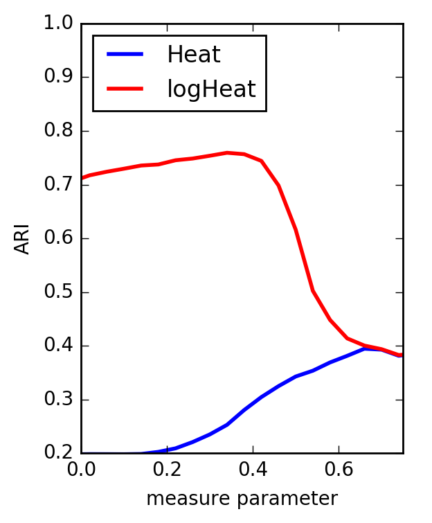
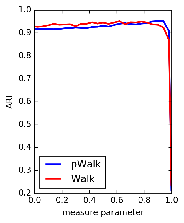
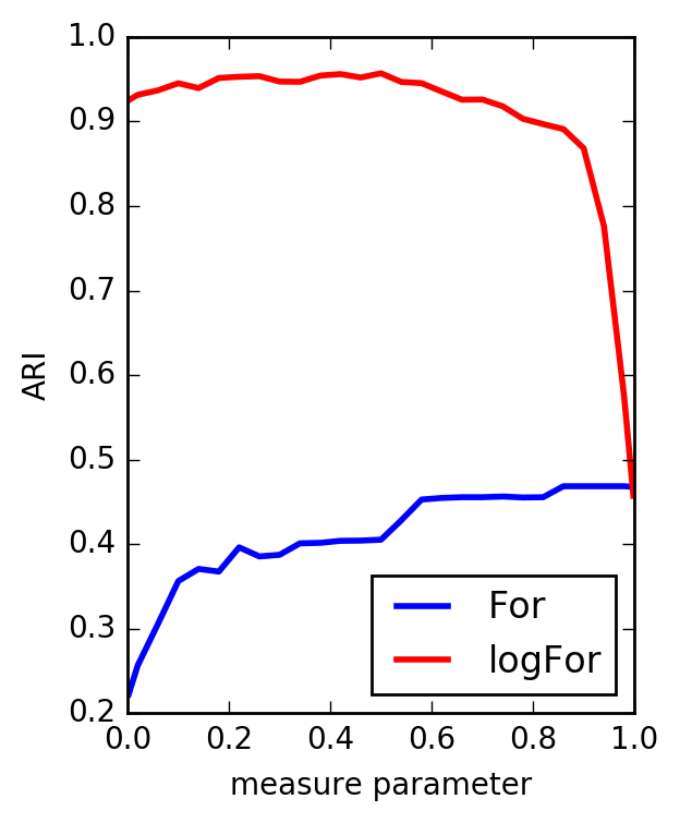
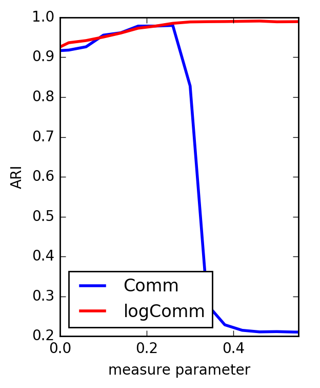
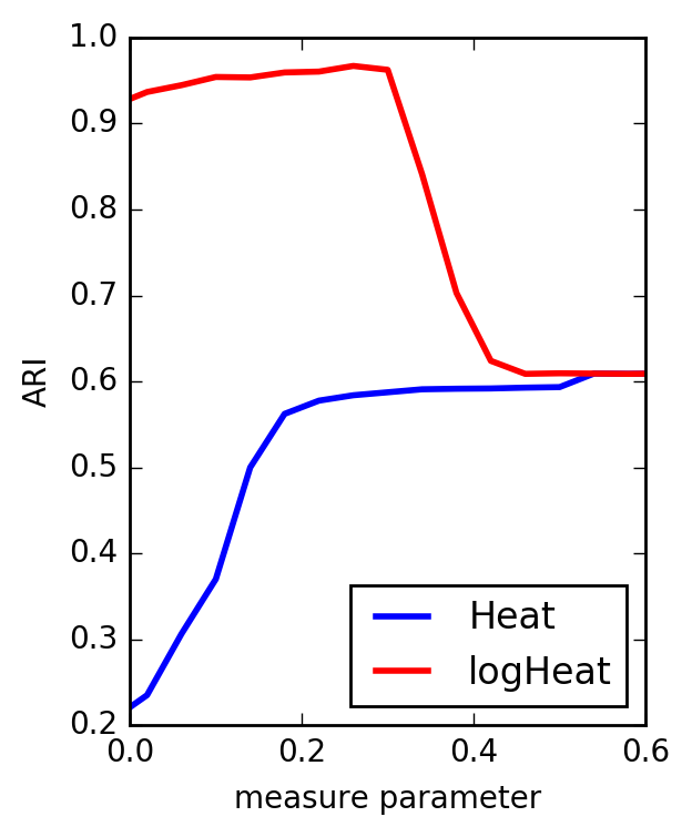
The curves in Figures 1–3 present the adjusted Rand index222On Rand index (RI) and adjusted Rand index (ARI) we refer to HubertArabie85 . (averaged over 200 random graphs) for clustering with Ward’s method Ward63JASA .
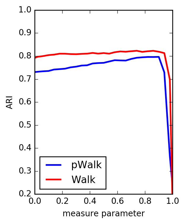
(a) plain Walk and Walk
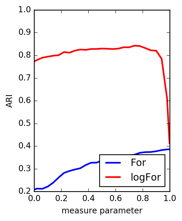
(b) Forest and logarithmic Forest
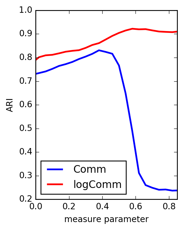
(c) (log)Communicability
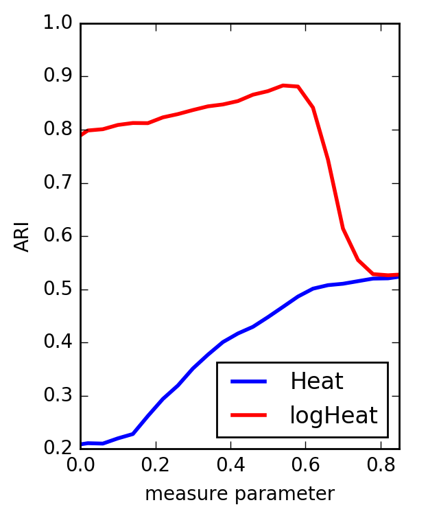
(d) Heat and logarithmic Heat
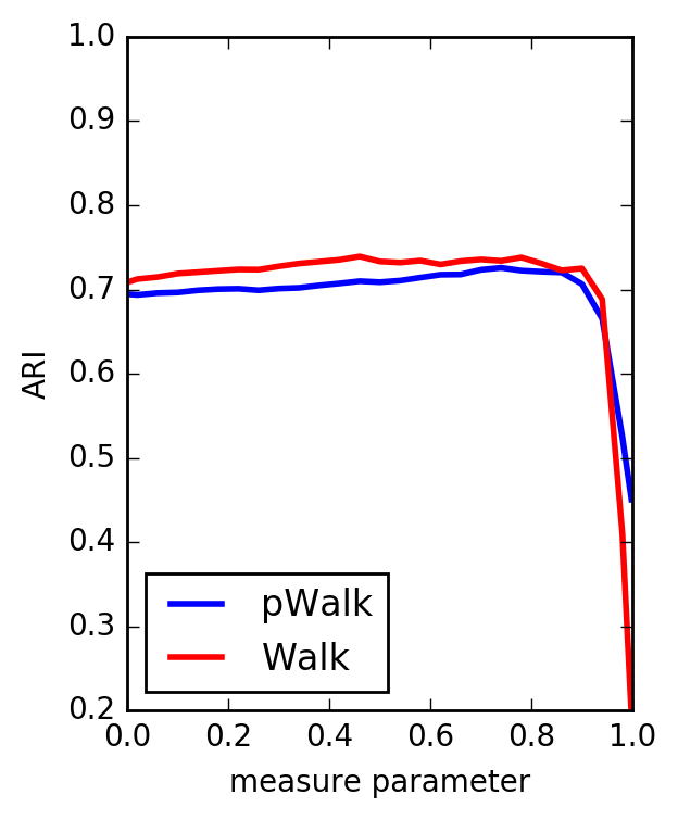
(a) plain Walk and Walk
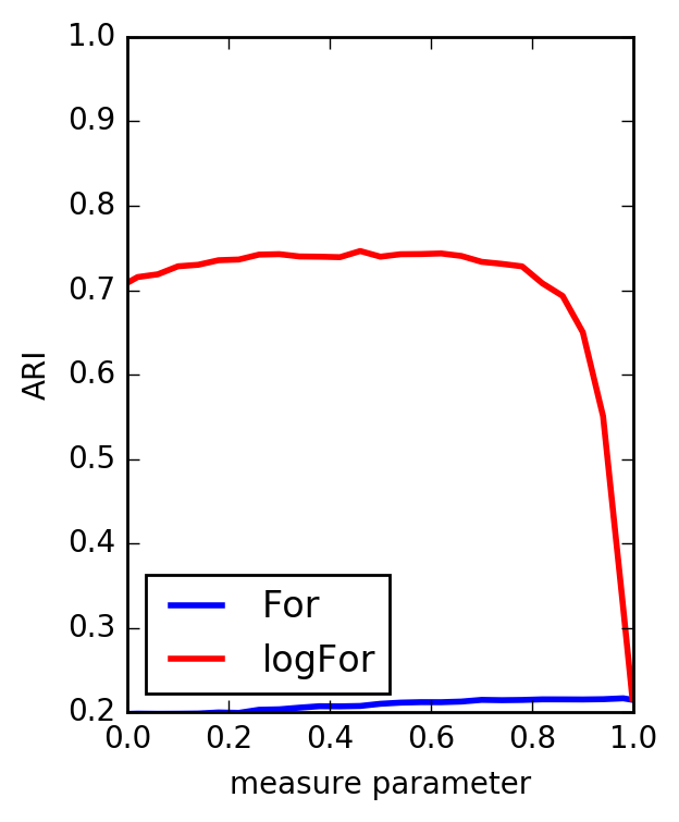
(b) Forest and logarithmic Forest
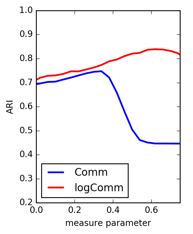
(c) (log)Communicability
(d) Heat and logarithmic Heat
(a) plain Walk and Walk
(b) Forest and logarithmic Forest
(c) (log)Communicability
(d) Heat and logarithmic Heat
It can be seen that in almost all cases, logarithmic measures outperform the ordinary ones. The only exception, where the situation is ambiguous, is the case of Walk measures for random graphs on 200 nodes.
3 Competition by Copeland’s score
In this section, we present the results of many clustering tests in the form of tournaments whose participants are the measure families. Every family is characterized by its Copeland’s score, i.e., the difference between the numbers of “wins” and “losses” in paired confrontations with the other families.
3.1 Approach Kivimaki2014developments
-
•
The competition of measure families is based on paired comparisons.
-
•
Every time when the best adjusted Rand index (ARI) of a measure family is higher on a random test graph than that of some other measure family , we add to the score of and to the score of .
3.2 The competition results
The competition has been performed on random graphs generated with the model and the following parameters: . For every combination of parameters, we generated 50 graphs and for each of them we computed the best ARI’s the measure families reached. The results are presented in Table 1(a).
3.3 A competition for 90th percentiles
Whenever we are looking for the best parameter of a measure family, we compute ARI on a grid of that parameter. In the above competition, we only compared the highest ARI values. Now consider the set of ARI values some measure family provides as a sample and find its 90th percentile. These percentiles become the participants in another tournament. The motivation behind this approach is to take into account the robustness of each family.
The results of the competition for 90th percentiles are given in Table 1(b).
| Nodes | 100 | 100 | 100 | 100 | 200 | 200 | 200 | 200 | Sum |
|---|---|---|---|---|---|---|---|---|---|
| Classes | 2 | 2 | 4 | 4 | 2 | 2 | 4 | 4 | of |
| 0.1 | 0.15 | 0.1 | 0.15 | 0.1 | 0.15 | 0.1 | 0.15 | scores | |
| logComm | 404 | 539 | 453 | 391 | 235 | 578 | 598 | 590 | |
| SCCT | 298 | 299 | 341 | 275 | 297 | 415 | 454 | 454 | |
| logFor | 154 | 182 | 202 | 226 | 207 | 44 | 226 | 192 | |
| logHeat | 249 | 261 | 140 | 28 | 175 | 302 | 251 | ||
| FE | 71 | 88 | 161 | 208 | 77 | 63 | 82 | 160 | |
| Comm | 120 | 9 | 27 | 267 | 138 | 156 | 84 | ||
| Walk | 130 | 185 | 126 | 49 | 138 | ||||
| pWalk | 64 | 109 | 76 | ||||||
| SCT | |||||||||
| RSP | 17 | ||||||||
| Heat | |||||||||
| SP-CT | |||||||||
| For |
(a) optimal parameters
| Nodes | 100 | 100 | 100 | 100 | 200 | 200 | 200 | 200 | Sum |
|---|---|---|---|---|---|---|---|---|---|
| Classes | 2 | 2 | 4 | 4 | 2 | 2 | 4 | 4 | of |
| 0.1 | 0.15 | 0.1 | 0.15 | 0.1 | 0.15 | 0.1 | 0.15 | scores | |
| logComm | 471 | 563 | 497 | 472 | 440 | 588 | 591 | 590 | |
| SCCT | 412 | 448 | 446 | 382 | 470 | 450 | 495 | 498 | |
| logFor | 171 | 242 | 275 | 166 | 88 | 185 | 296 | 210 | |
| Walk | 229 | 291 | 268 | 48 | 145 | 226 | 320 | ||
| pWalk | 19 | 45 | 221 | 232 | 113 | 111 | 188 | 217 | |
| FE | 91 | 95 | 240 | 56 | 18 | 152 | |||
| logHeat | 342 | 91 | 269 | 156 | 61 | ||||
| SCT | |||||||||
| Comm | 2 | 10 | |||||||
| SP-CT | |||||||||
| RSP | |||||||||
| Heat | |||||||||
| For |
(b) 90th percentiles
One can notice a number of differences between the orders of families provided by the first competition and the second one. However, in both cases, logarithmic measures outperform the corresponding plain ones. In particular, it can be observed that FE is also a kind of logarithmic measure, as distinct from RSP.
Here, the undisputed leader is logComm. Second place goes to SCCT, a measure which is not logarithmic, but involves even a more smoothing sigmoid transformation.
4 Reject curves
In this section, we compare the performance of distances (corresponding to the proximity measures or defined independently) in clustering tasks using reject curves.
4.1 Definition
The ROC curve (also referred to as the reject curve) for this type of data can be defined as follows.
-
•
Let us order the distances from the minimum to the maximum, where the distance corresponding to a kernel is produced by the transformation333Recall that a number of distances that correspond to logarithmic measures possess a meaningful cutpoint additivity property Che13Paris ..
-
•
To each we assign a point in the square. Its -coordinate is the share of inter-class distances that are less than or equal to the -coordinate being the share of intra-class distances (between different nodes) that are less than or equal to
-
•
The polygonal line connecting the consecutive points is the reject curve corresponding to the graph.
A better measure is characterized by a reject curve that goes higher or, at least, has a larger area under the curve.
4.2 Results
The optimal values of the family parameters (adjusted to the segment) w.r.t. the ARI in clustering based on Ward’s method for three models are presented in Table 2.
| Measure | |||
|---|---|---|---|
| (kernel) | Opt. parameter, ARI | Opt. parameter, ARI | Opt. parameter, ARI |
| pWalk | 0.86, 0.9653 | 0.90, 0.8308 | 0.66, 0.5298 |
| Walk | 0.86, 0.9664 | 0.74, 0.8442 | 0.64, 0.5357 |
| For | 1.00, 0.5816 | 0.98, 0.3671 | 0.00, 0.2007 |
| logFor | 0.62, 0.9704 | 0.56, 0.8542 | 0.52, 0.5541 |
| Comm | 0.38, 0.9761 | 0.32, 0.8708 | 0.26, 0.5661 |
| logComm | 0.68, 0.9838 | 0.54, 0.9466 | 0.62, 0.7488 |
| Heat | 0.86, 0.6128 | 0.86, 0.5646 | 0.78, 0.2879 |
| logHeat | 0.52, 0.9827 | 0.40, 0.8911 | 0.28, 0.5561 |
| SCT | 0.74, 0.9651 | 0.62, 0.8550 | 0.64, 0.5531 |
| SCCT | 0.36, 0.9834 | 0.26, 0.9130 | 0.22, 0.6626 |
| RSP | 0.99, 0.9712 | 0.98, 0.8444 | 0.98, 0.5430 |
| FE | 0.94, 0.9697 | 0.94, 0.8482 | 0.86, 0.5460 |
| SP-CT | 0.28, 0.9172 | 0.34, 0.6782 | 0.42, 0.4103 |
The optimum chosen on the grid of 50 parameter values is shown as the first number in each of three columns. The second number is the ARI corresponding to the optimum averaged over 200 random graphs. The maximum averaged ARI’s are underlined. All of them belong to logComm.
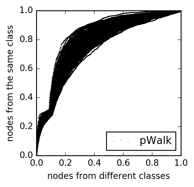
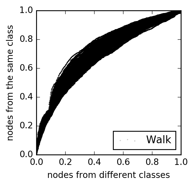
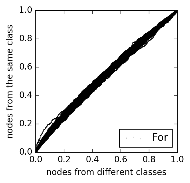
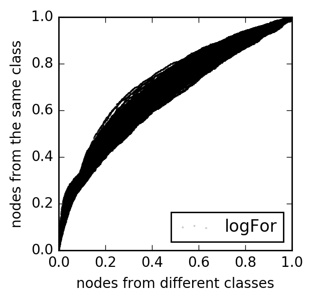
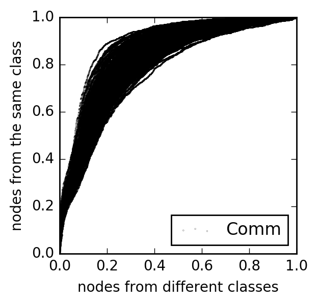
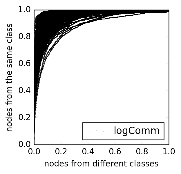
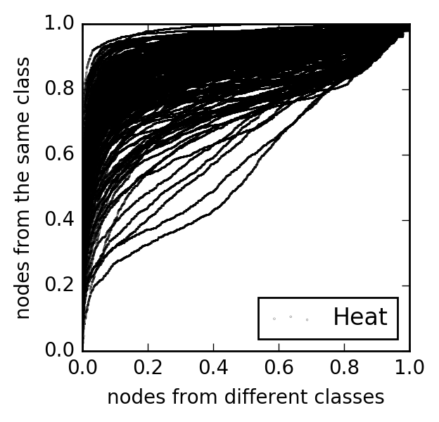
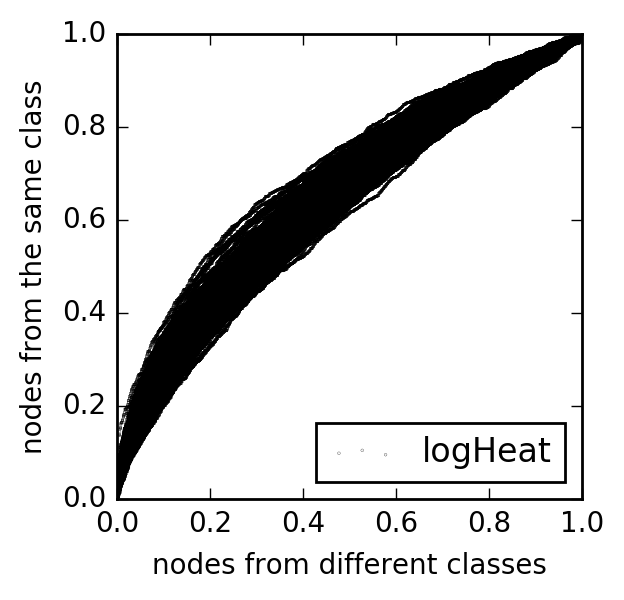
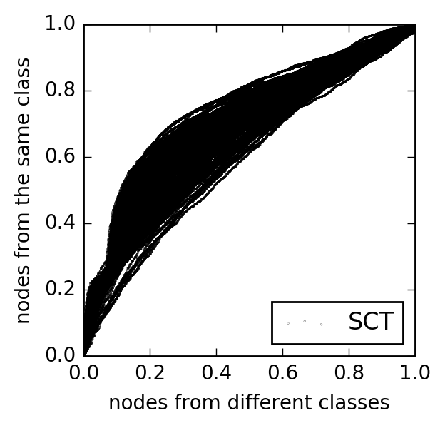
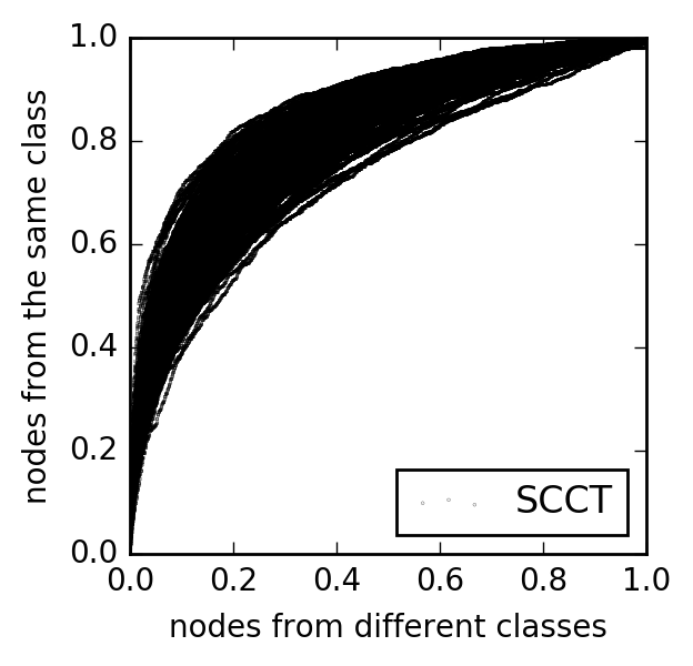
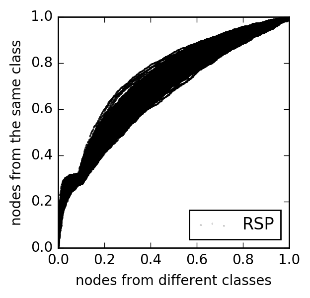
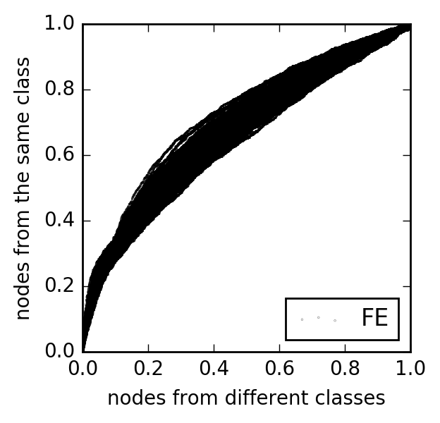
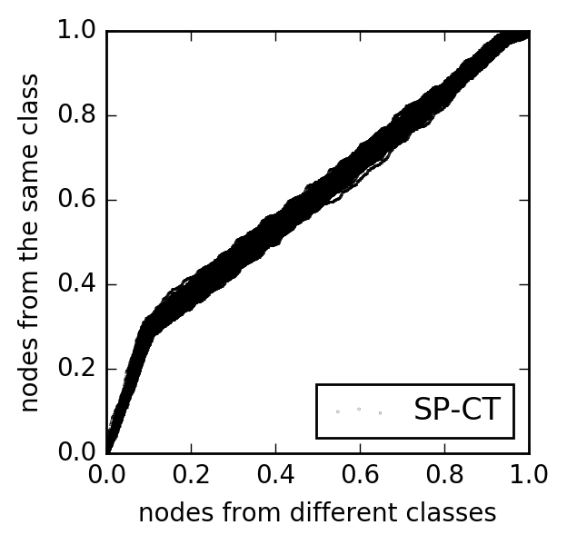
The reject curves for and the optimal values of the family parameters (w.r.t. the ARI of Ward’s method clustering) are shown in Fig.4. Each subfigure contains 200 lines corresponding to 200 random graphs.
(a) pWalk
(b) Walk
(c) For
(d) logFor
(e) Comm
(f) logComm
(g) Heat
(h) logHeat
(i) SCT
(j) SCCT
(k) RSP
(l) FE
(m) SP-CT
The -like bend of several curves (pWalk, Walk, logFor, SCT, RSP, FE) appears because the corresponding measures strongly correlate with the Shortest path (SP) distance between nodes. In these experiments, the SP distance takes only a few small values.
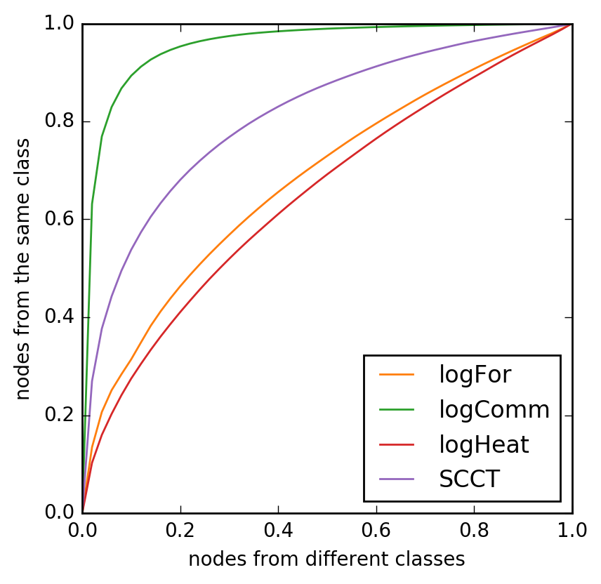
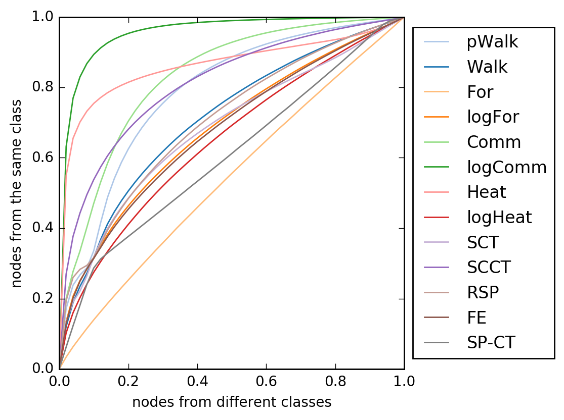
Finally, in Fig. 5(a) we show the reject curves averaged over 200 random graphs. The curves for the four families that are leaders in Table 1 are duplicated in Fig. 5(b).
(a) All families
One can observe that the results are partially concordant with those obtained with Ward’s method. In particular, the first place goes to logComm. Therefore, these results are not an exclusive feature of Ward’s method. Notice that Heat has a good average reject curve. However, it produces relatively many large intra-class distances and its partial results are extremely unstable. This supposedly determines the low values of ARI of this measure.
5 Graphs with classes of different sizes
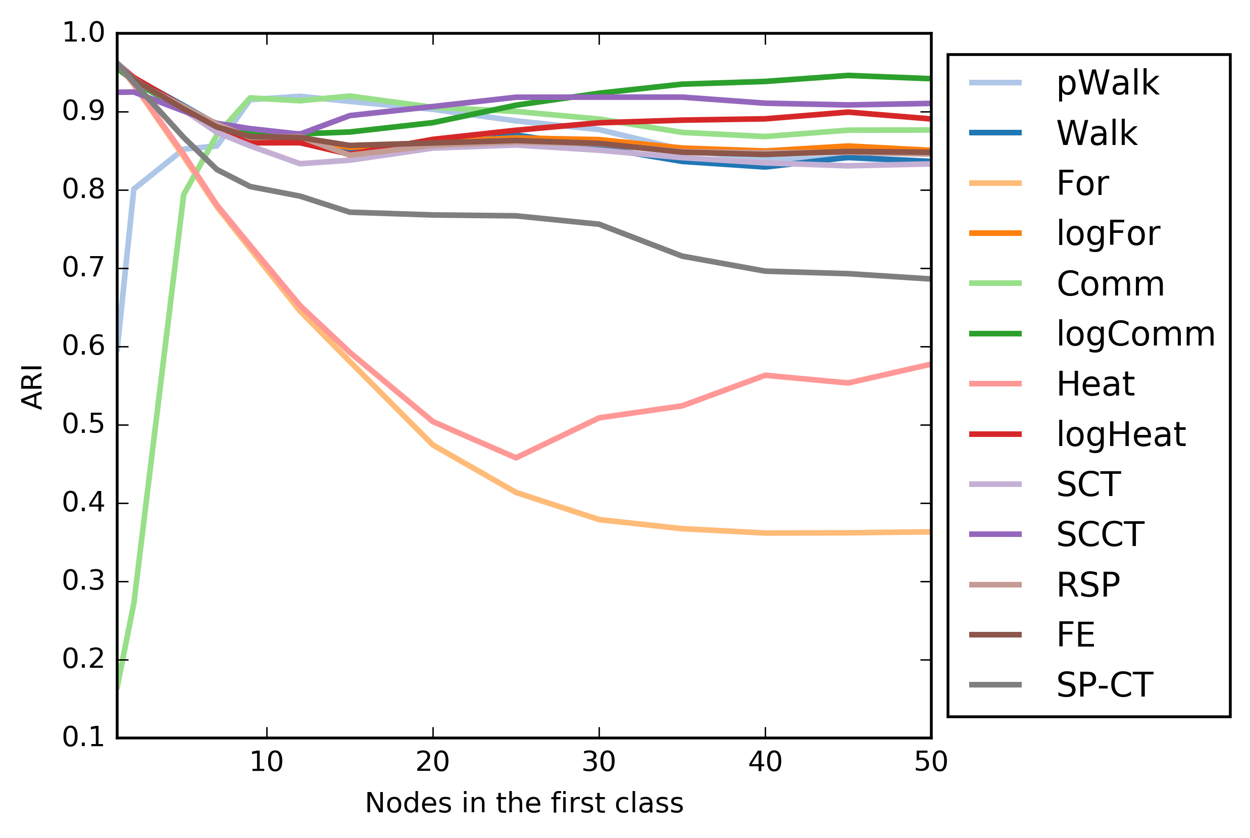
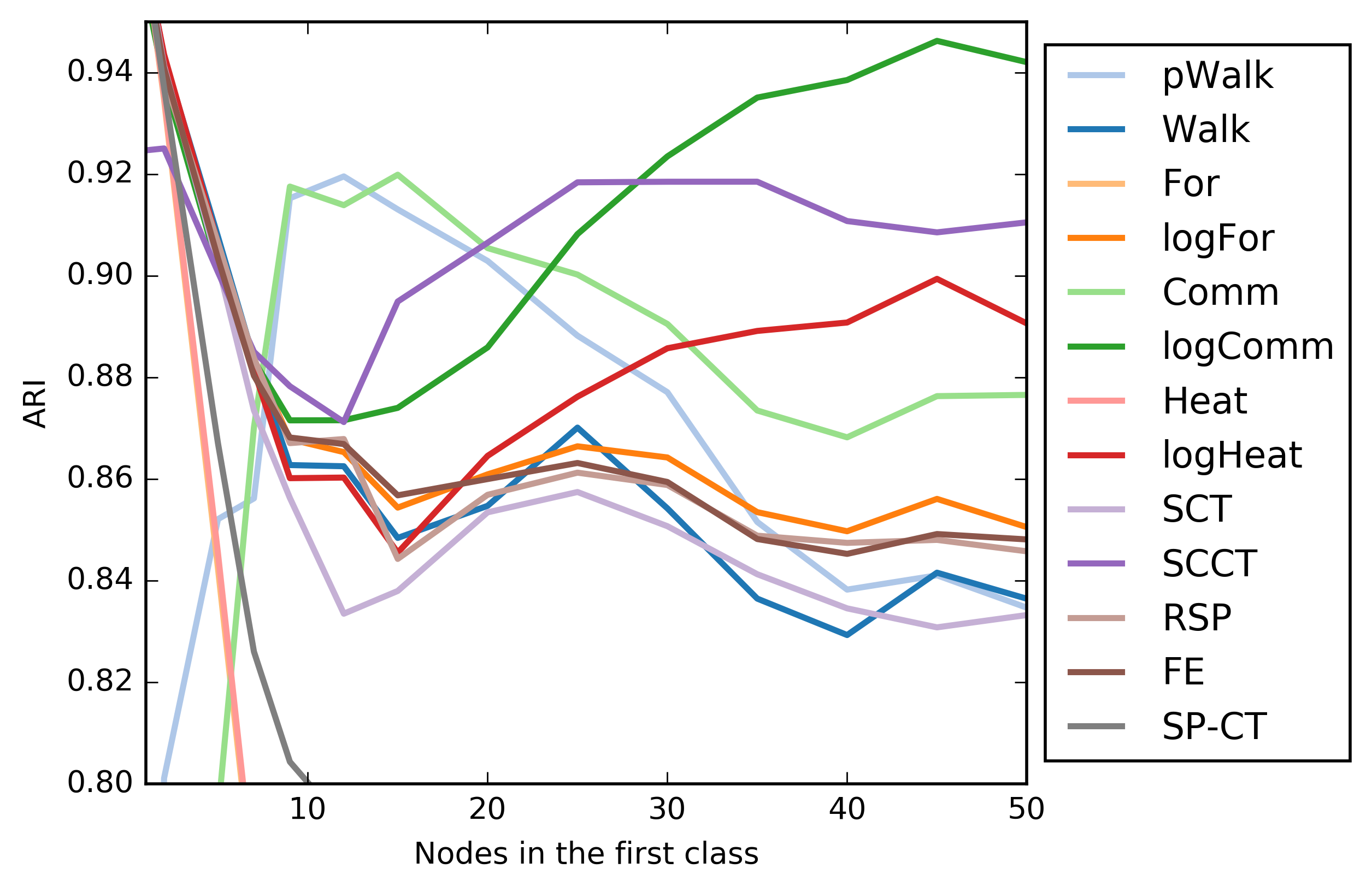
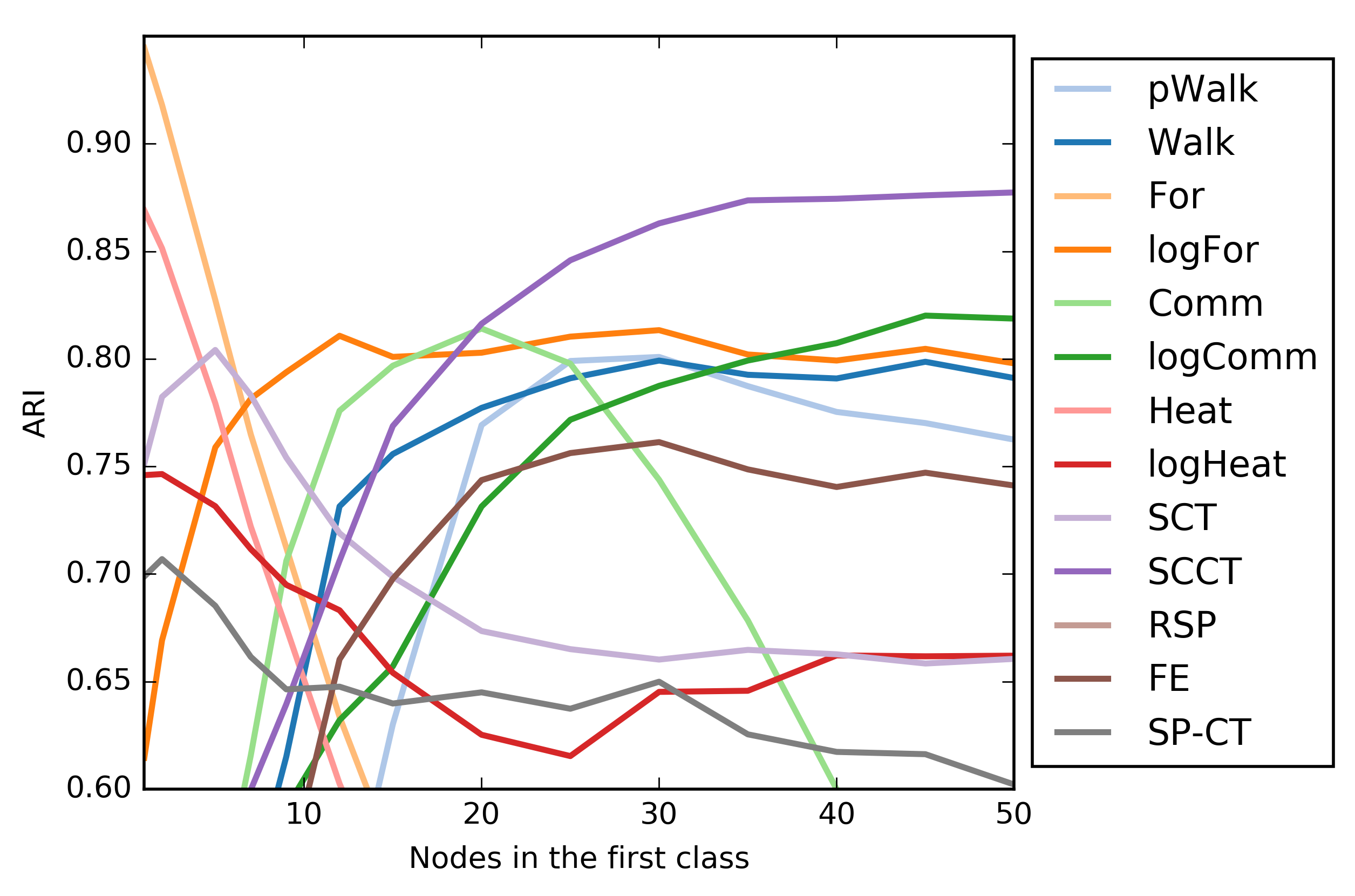
The model generates graphs with nodes divided into classes of the same size. We now consider graphs with nodes divided into two classes of different sizes. The size of the first class, , is shown along the horizontal axis in Fig. 6.
(a) All families
(b) Leading families
We see that the ARI’s of logComm, SCCT, and logHeat have minima at near or In contrast, the ARI’s of Comm and pWalk have larger maxima in the same interval. As a result, the latter two measures outperform the former three (and the other measures under study) at However, if is very small, then Ward’s method with Comm or pWalk seems to engender misrecognition. Thus, this case can be considered as an exception to the rule that “logarithmic measures outperform plain ones”: with a moderate size of the smaller class, Comm and pWalk outperform the logarithmic measures (and also SCCT in which the sigmoid function is analogous to the logarithmic one as a smoothing transformation).
In all the above experiments, we looked for the optimal values of the family parameters. If the families of measures are used with random parameter values, then the rating of the families differs. Now, the leader and the vice-leader are SCCT and logFor, respectively, which are most robust to the variation of the family parameter; when one class is very small, the winners are For, SCT, and Heat, see Fig. 7.
Now let us consider a highly heterogeneous data structure: 150 nodes are divided into six classes whose sizes are 65, 35, 25, 13, 8, and 4. The classes are numbered in the descending order of size. The probability of an edge connecting two vertices that belong to classes and is the entry of the matrix
![[Uncaptioned image]](/html/1605.01046/assets/AddFigures/sixClusters.png) \twocaptionwidth
\twocaptionwidth
.45.45\rightcaptionARI of various measure families on a structure with 6 classes
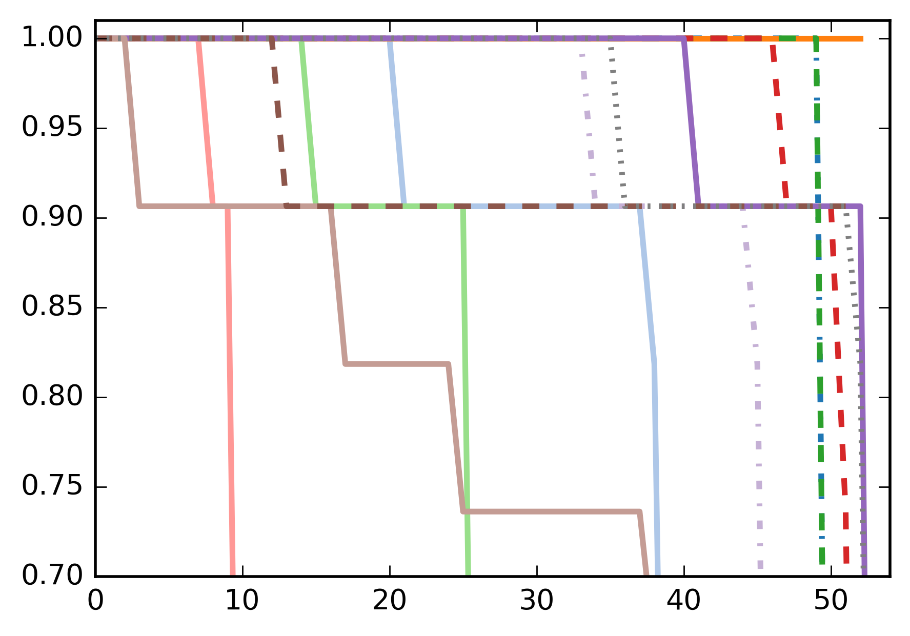
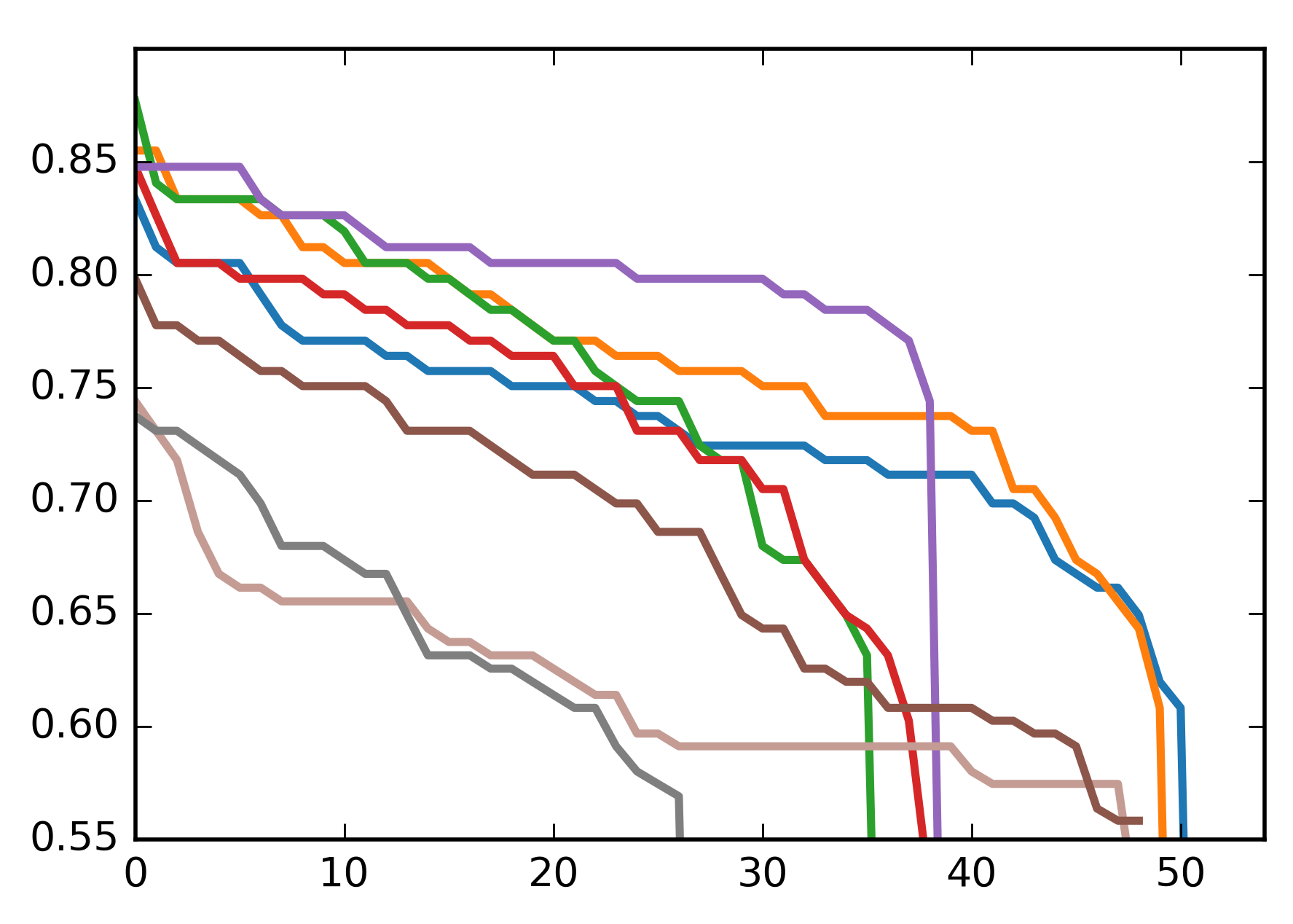
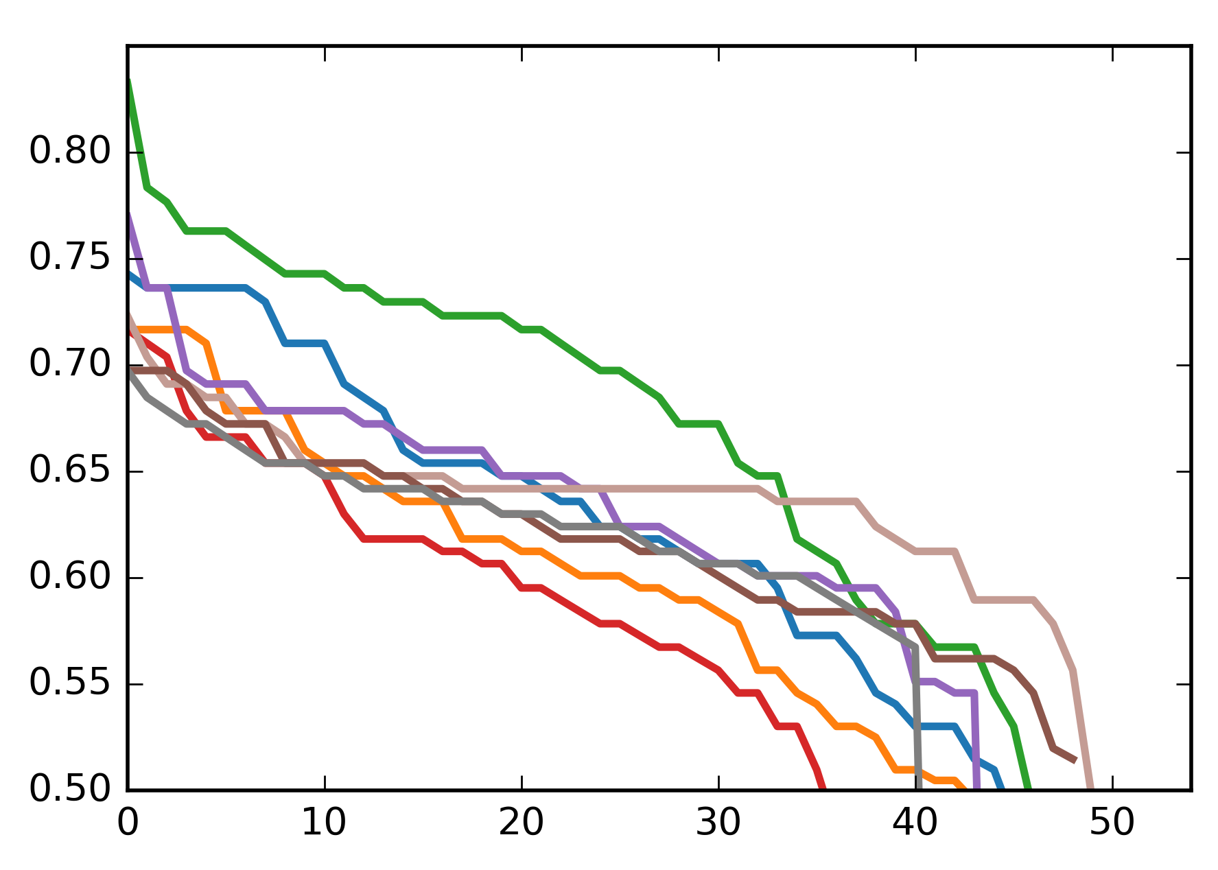
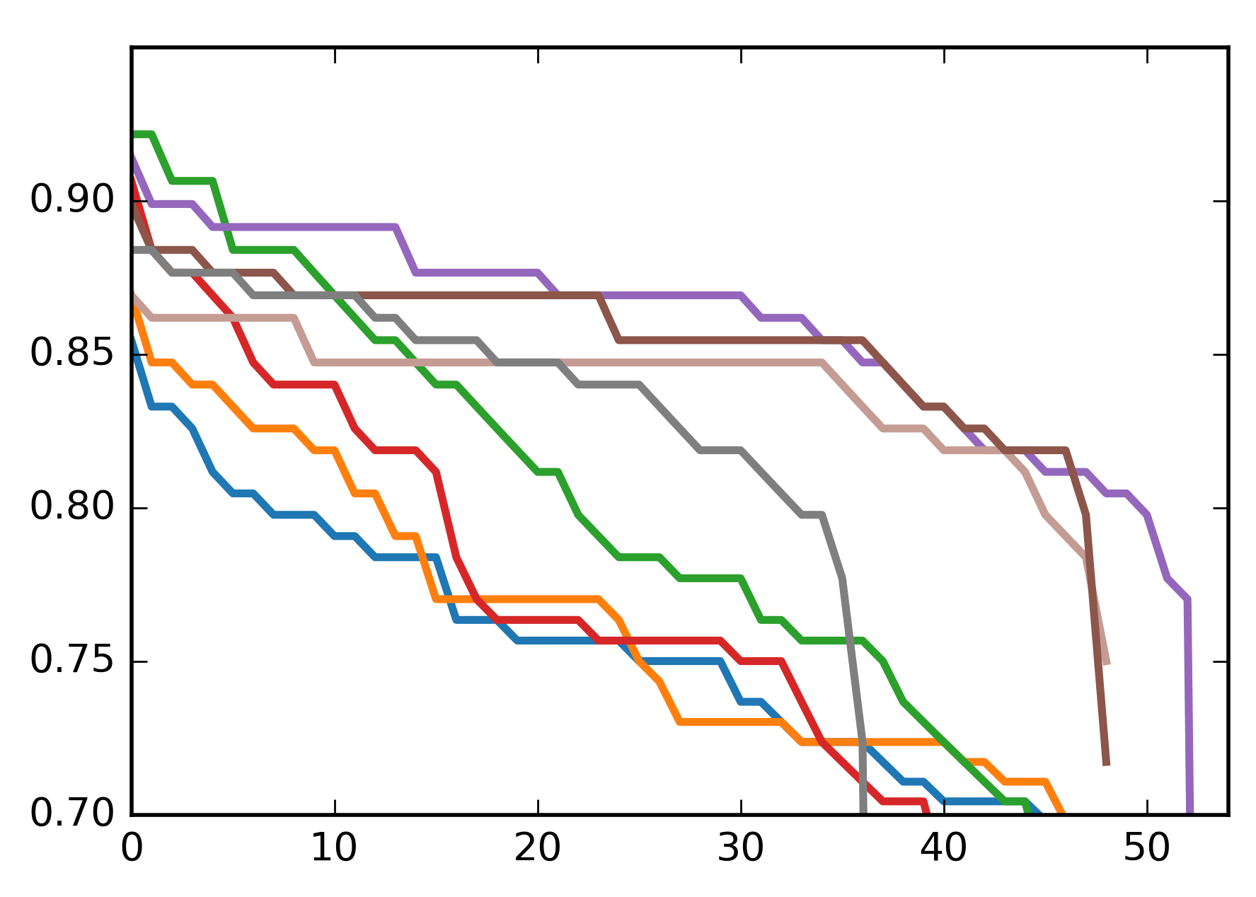
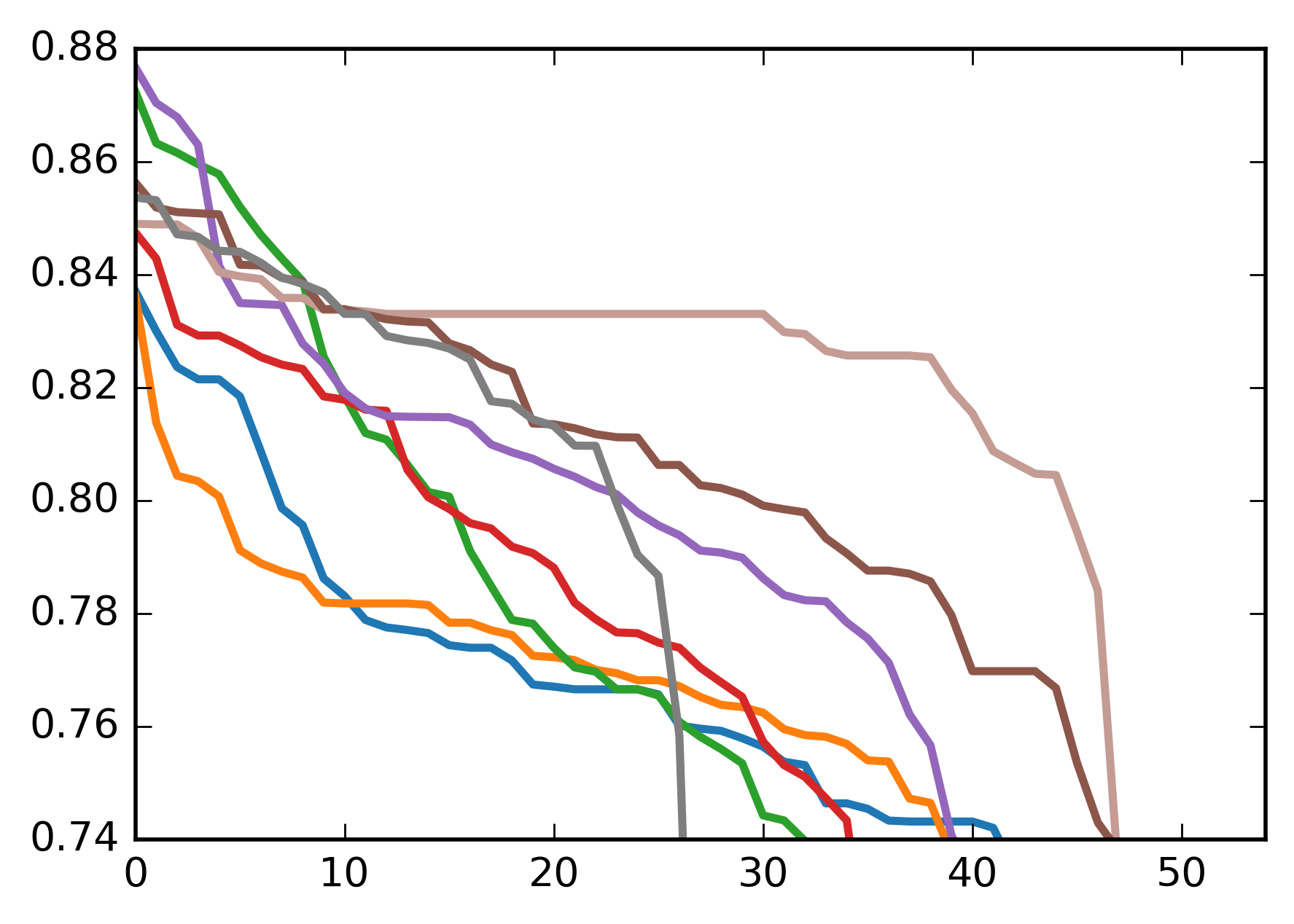
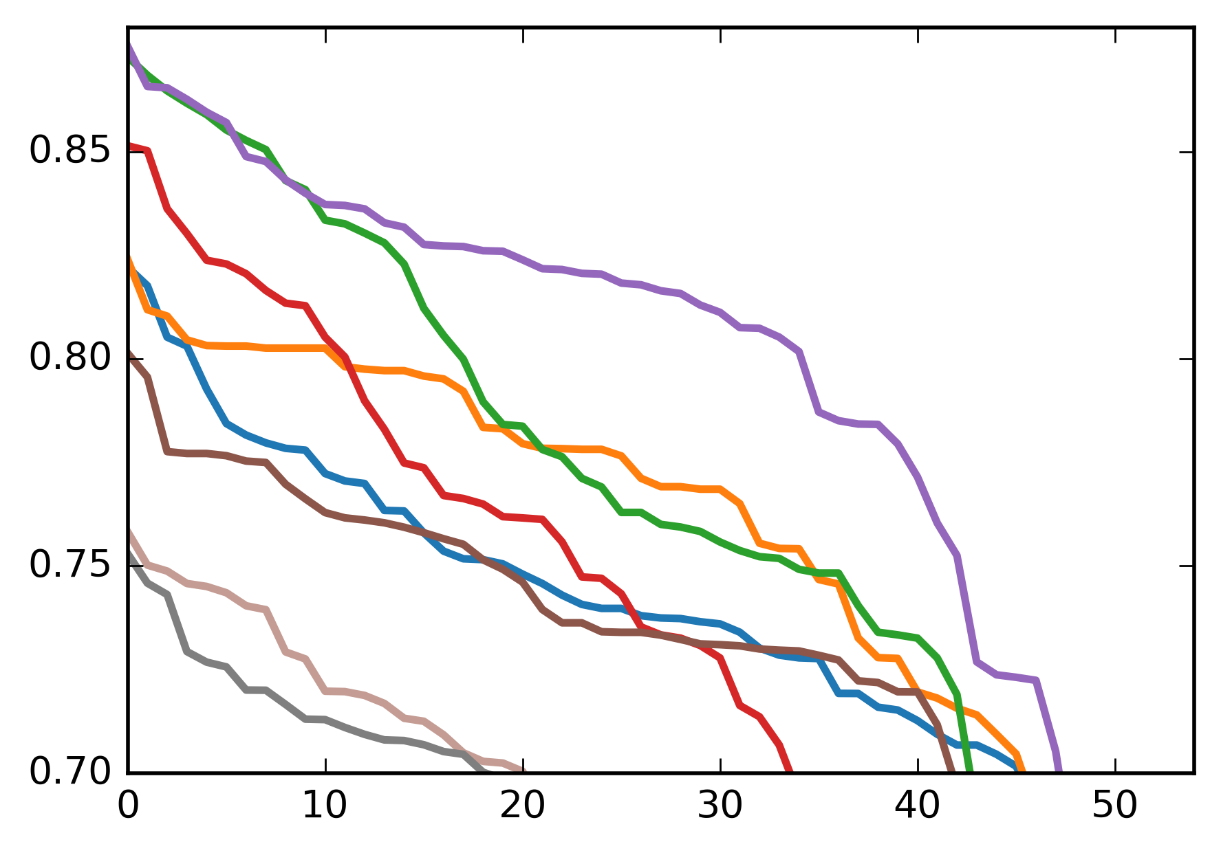
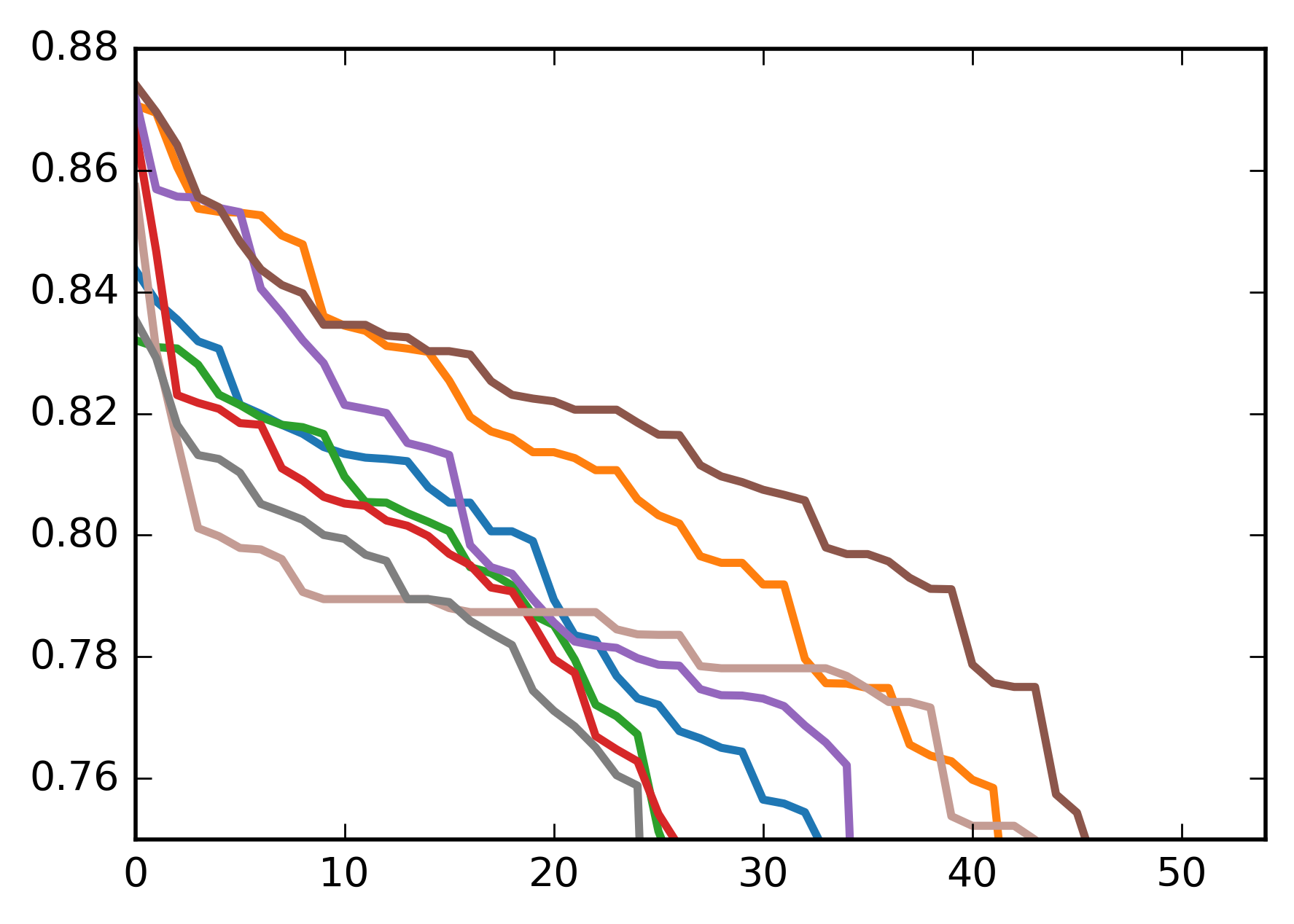
For each measure family, we considered 55 values of the family parameter and sorted them in the descending order of the corresponding ARI averaged for 200 random graphs. ARI against the rank of the family parameter value is shown in Fig. 5. Two things are important for each family: first, the maximum of ARI and second, the velocity of descent.
For this data structure, the leaders are Comm and pWalk, as well as for the two-component graphs with one small, but not very small class of nodes.
6 Cluster analysis on several classical datasets
Hitherto we mainly considered one type of random graph: the graphs with uniform interclass edge probabilities and uniform intraclass edge probabilities. Certainly, many real-world graphs can hardly be obtained in the framework of that model. In this section, we study clustering on several datasets frequently used to check various graph algorithms.
We investigate a total of 9 graphs, the smallest of which (Zachary’s Karate club zachary1977information ) contains 34 nodes. The largest graph (a Newsgroup graph YenFoussSaerens09 with three classes) contains 600 nodes. We analyse six Newsgroup datasets. The remaining datasets are Football girvan2002community and Political books newman2006modularity . Table 3 presents some features of the datasets.
| Dataset family | Dataset name | Number of nodes | Number of classes |
|---|---|---|---|
| Football | football | 115 | 12 |
| Political books | polbooks | 105 | 3 |
| Zachary | Zachary | 34 | 2 |
| Newsgroup | news_2cl_1 | 400 | 2 |
| news_2cl_2 | 400 | 2 | |
| news_2cl_3 | 400 | 2 | |
| news_3cl_1 | 600 | 3 | |
| news_3cl_2 | 600 | 3 | |
| news_3cl_3 | 600 | 3 |
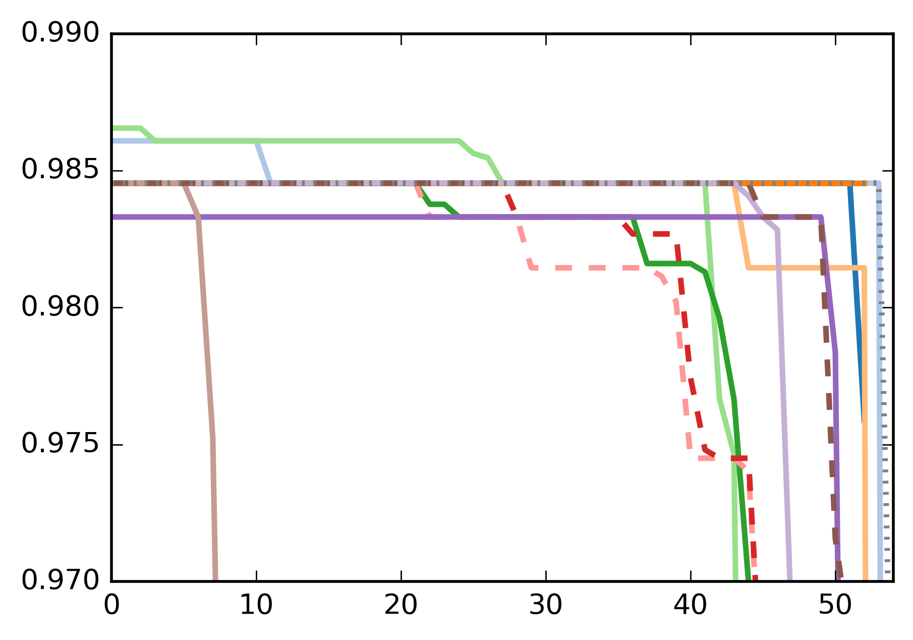
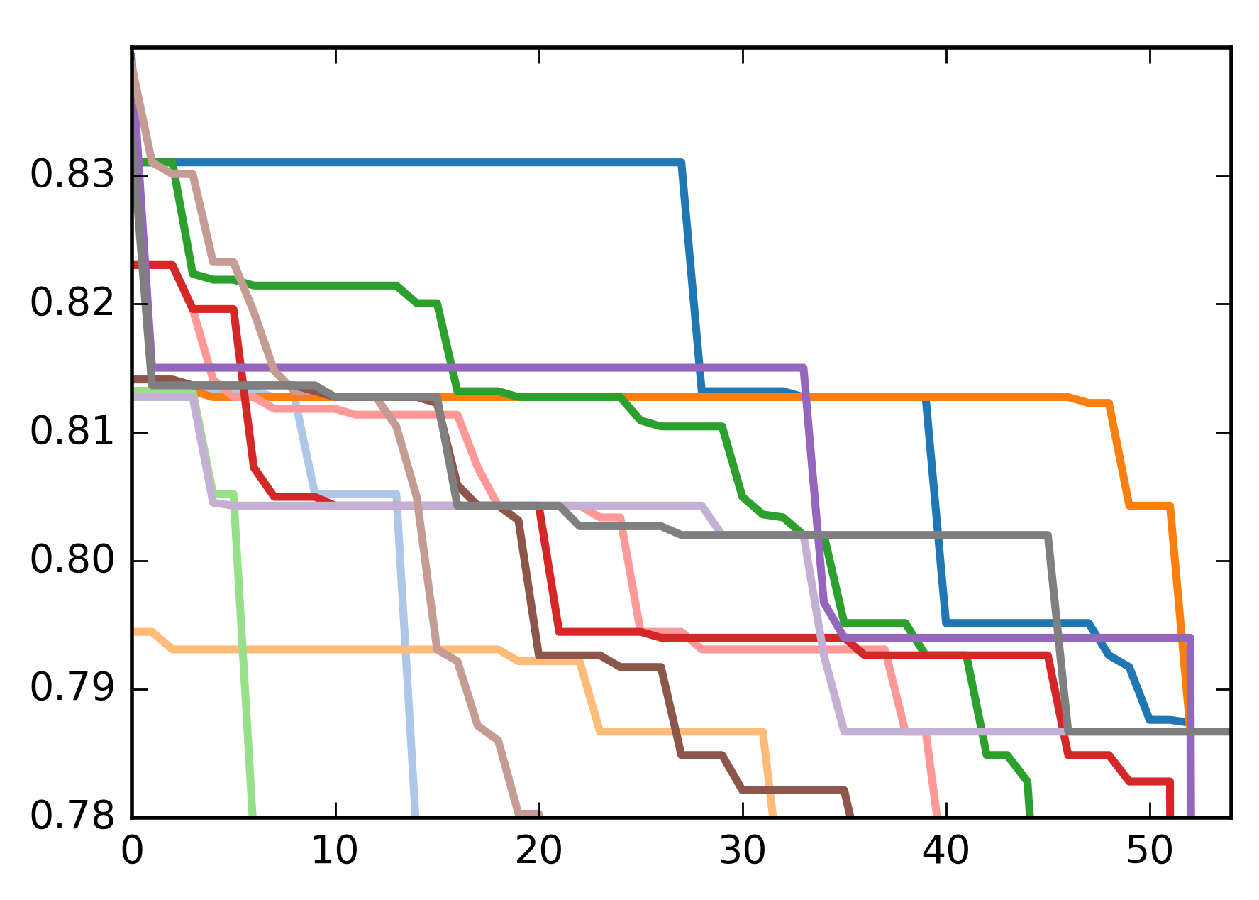
For each dataset and each measure family, we sorted 55 values of the family parameter in the descending order of the corresponding ARI. ARI against the rank of the family parameter value is shown in Fig. 8.
(a) football
(b) polbooks
(c) Zachary
(d) news_2cl_1
(e) news_2cl_2
(f) news_2cl_3
(g) news_3cl_1
(h) news_3cl_2
(i) news_3cl_3

Finally, we present Copeland’s score competition for the measure families: separately for the best values of the family parameters and for 80th percentiles (Tables 4 and 5).
One can observe that for different datasets, ranking of measure families w.r.t. the quality of clustering differs. In Table 4, for six datasets, SCCT takes the 1st or 2nd place; logComm does so for five datasets. In most cases, the logarithmic measures outperform the corresponding plain ones. For the “news_3cl_3” dataset and 80th percentiles, the leaders are FE and logFor. For “Zachary” with the best parameter, all measures, except for For, reach an absolute result. For “football” (having 12 classes), Comm and pWalk are the winners with the best parameters, like in the cases of two classes of different sizes (cf. Fig. 6(b)) and of six classes (Fig. 5); SCCT is the worst.
The comparison of Tables 4 and 5 demonstrates that the rather high results of logHeat and RSP are not stable enough, so in the ranking with 80th percentiles, they lose four and three positions, respectively; Walk, logFor and SP-CT shift up two places each. This dynamics resembles that in Table 1(a), (b).
7 Conclusion
The main conclusion of our study is that in most cases, including the simple cases of random graphs with homogeneous classes of similar size, logarithmic measures (i.e., measures resulting after taking logarithm of the proximities) better reveal the underlying structure than the “plain” measures do. A direct comparison of inter-class and intra-class distances by drawing the reject curves confirms this conclusion (with the exception of Heat and logHeat).
In our experiments, the three leading measure families in the aforementioned simple cases, according to Copelands’s test presented in Table 1, are logarithmic Communicability, Sigmoid Corrected Commute Time kernel, and logarithmic Forest. The superiority of logarithmic Communicability over the other measures is observed here for all sets of random graphs, except for the set for which SCCT is the best.
A plausible explanation of the superiority of logarithmic measures is that most kernels and proximity measures under study have a multiplicative nature, while the nature of distances that cluster algorithms actually use is an additive one (as the triangle inequality reveals). The logarithmic transformation is precisely the tool that transforms the first nature to the second one. Moreover, some distances corresponding to the logarithmic measures possess a meaningful cutpoint additivity property.
At the same time, there are more complex heterogeneous networks for which other measures can behave well. Among such structures, we can mention one type of networks with classes of different sizes and smaller classes of moderate sizes, for which two “plain” measures, Comm and pWalk can outperform the logarithmic measures under study. A similar situation can be observed for some structures with many classes. The SCCT kernel, which involves the sigmoid transformation instead of the logarithmic one, performs very well in many experiments. In Ward’s clustering (with the best parameter values) of several datasets, it even wins in the competition by Copeland’s score.
References
- (1) Buckley, F., Harary, F.: Distance in Graphs. Addison-Wesley, Redwood City, CA (1990)
- (2) Chandra, A.K., Raghavan, P., Ruzzo, W.L., Smolensky, R., Tiwari, P.: The electrical resistance of a graph captures its commute and cover times. In: Proc. 21st Annual ACM Symp. on Theory of Computing, pp. 574–586. ACM Press, Seattle (1989)
- (3) Chebotarev, P.: A class of graph-geodetic distances generalizing the shortest-path and the resistance distances. Discrete Applied Mathematics 159(5), 295–302 (2011)
- (4) Chebotarev, P.: The graph bottleneck identity. Advances in Applied Mathematics 47(3), 403–413 (2011)
- (5) Chebotarev, P.: The walk distances in graphs. Discrete Applied Mathematics 160(10–11), 1484–1500 (2012)
- (6) Chebotarev, P.: Studying new classes of graph metrics. In: F. Nielsen, F. Barbaresco (eds.) Proceedings of the SEE Conference “Geometric Science of Information” (GSI-2013), Lecture Notes in Computer Science, LNCS 8085, pp. 207–214. Springer, Berlin (2013)
- (7) Chebotarev, P., Shamis, E.: The forest metrics for graph vertices. Electronic Notes in Discrete Mathematics 11, 98–107 (2002)
- (8) Chebotarev, P.Y., Shamis, E.V.: The matrix-forest theorem and measuring relations in small social groups. Automation and Remote Control 58(9), 1505–1514 (1997)
- (9) Chebotarev, P.Y., Shamis, E.V.: On a duality between metrics and -proximities. Automation and Remote Control 59(4), 608–612 (1998)
- (10) Chebotarev, P.Y., Shamis, E.V.: On proximity measures for graph vertices. Automation and Remote Control 59(10), 1443–1459 (1998)
- (11) Chung, F., Yau, S.T.: Coverings, heat kernels and spanning trees. Journal of Combinatorics 6, 163–184 (1998)
- (12) Collette, A.: Comparison of some community detection methods for social network analysis. Master’s thesis, Louvain School of Management, Universite catholique de Louvain, Louvain, Belgium (2015). 80 pp.
- (13) Estrada, E.: The communicability distance in graphs. Linear Algebra and its Applications 436(11), 4317–4328 (2012)
- (14) Fortunato, S.: Community detection in graphs. Physics reports 486(3), 75–174 (2010)
- (15) Fouss, F., Francoisse, K., Yen, L., Pirotte, A., Saerens, M.: An experimental investigation of kernels on graphs for collaborative recommendation and semisupervised classification. Neural Networks 31, 53–72 (2012)
- (16) Fouss, F., Saerens, M., Shimbo, M.: Algorithms and Models for Network Data and Link Analysis. Cambridge University Press (2016)
- (17) Girvan, M., Newman, M.E.J.: Community structure in social and biological networks. Proceedings of the National Academy of Sciences 99(12), 7821–7826 (2002)
- (18) Göbel, F., Jagers, A.A.: Random walks on graphs. Stochastic Processes and their Applications 2(4), 311–336 (1974)
- (19) Gvishiani, A.D., Gurvich, V.A.: Metric and ultrametric spaces of resistances. Russian Mathematical Surveys 42(6), 235–236 (1987)
- (20) Hubert, L., Arabie, P.: Comparing partitions. Journal of Classification 2(1), 193–218 (1985)
- (21) Kandola, J., Cristianini, N., Shawe-Taylor, J.S.: Learning semantic similarity. In: Advances in neural information processing systems, pp. 657–664 (2002)
- (22) Kivimäki, I., Shimbo, M., Saerens, M.: Developments in the theory of randomized shortest paths with a comparison of graph node distances. Physica A: Statistical Mechanics and its Applications 393, 600–616 (2014)
- (23) Klein, D.J., Randić, M.: Resistance distance. Journal of Mathematical Chemistry 12, 81–95 (1993)
- (24) Kondor, R.I., Lafferty, J.: Diffusion kernels on graphs and other discrete structures. In: Proceedings of the 19th international conference on machine learning, pp. 315–322 (2002)
- (25) von Luxburg, U., Radl, A., Hein, M.: Getting lost in space: Large sample analysis of the resistance distance. In: NIPS 2010, Twenty-Fourth Annual Conference on Neural Information Processing Systems, pp. 1–9. Curran, Red Hook, NY (2011)
- (26) Nash-Williams, C.S.J.A.: Random walk and electric currents in networks. Mathematical Proceedings of the Cambridge Philosophical Society 55(02), 181–194 (1959)
- (27) Newman, M.E.J.: Modularity and community structure in networks. Proceedings of the National Academy of Sciences 103(23), 8577–8582 (2006)
- (28) Saerens, M., Fouss, F., Yen, L., Dupont, P.: The principal components analysis of a graph, and its relationships to spectral clustering. In: Machine Learning: ECML 2004, pp. 371–383. Springer (2004)
- (29) Schaeffer, S.E.: Graph clustering. Computer Science Review 1(1), 27–64 (2007)
- (30) Sharpe, G.E.: Solution of the -terminal resistive network problem by means of metric geometry. In: Proceedings of the First Asilomar Conference on Circuits and Systems, pp. 319–328. Pacific Grove, CA (1967)
- (31) Smola, A.J., Kondor, R.I.: Kernels and regularization of graphs. In: Proceedings of the 16th Annual Conference on Learning Theory, pp. 144–158 (2003)
- (32) Sommer, F., Fouss, F., Saerens, M.: Comparison of graph node distances on clustering tasks, pp. 192–201. Lecture Notes in Computer Science, LNCS . Springer, Cham (2016)
- (33) Ward Jr, J.H.: Hierarchical grouping to optimize an objective function. Journal of the American Statistical Association 58(301), 236–244 (1963)
- (34) Yen, L., Fouss, F., Decaestecker, C., Francq, P., Saerens, M.: Graph nodes clustering with the sigmoid commute-time kernel: A comparative study. Data & Knowledge Engineering 68, 338–361 (2009)
- (35) Zachary, W.W.: An information flow model for conflict and fission in small groups. Journal of Anthropological Research pp. 452–473 (1977)
