The quantum computer puzzle
(Expanded Version)

Any new possibility that existence acquires, even the least likely, transforms everything about existence.

Milan Kundera – Slowness

Quantum computers are hypothetical devices, based on quantum physics, that would enable us to perform certain computations hundreds of orders of magnitude faster than digital computers [19, 17]. This feature is coined as “quantum supremacy” [51] and one aspect or another of such quantum computational supremacy might be brought about in experiments in the near future: by implementing quantum error-correction, systems of non-interacting bosons, exotic new phases of matter called anyons, quantum annealing, or in various other ways. We concentrate in this paper on the model of a universal quantum computer, which allows the full computational potential of quantum systems, and on the restricted model, called “BosonSampling,” based on non-interacting bosons.

A main concern regarding the feasibility of quantum computers is that quantum systems are inherently noisy: we cannot accurately control them, and we cannot accurately describe them. We will describe an optimistic hypothesis of quantum noise that would allow quantum computing and a pessimistic hypothesis that wouldn’t. The quantum computer puzzle is deciding between these two hypotheses. We list some remarkable consequences of the optimistic hypothesis, giving strong reasons for the intensive efforts to build quantum computers, as well as good reasons for suspecting that this might not be possible. For systems of non-interacting bosons, we explain how quantum supremacy achieved without noise is replaced, in the presence of noise, by a very low yet fascinating computational power (based on Kalai and Kindler [36]). Finally, based on the pessimistic hypothesis, we make seventeen predictions about quantum physics and computation (based on, Kalai [33], and a subsequent Internet debate with Aram Harrow and others).

Are quantum computers feasible? Is quantum supremacy possible? My expectation is that the pessimistic hypothesis will prevail, leading to a negative answer. Rather than regard this possibility as an unfortunate failure that impedes the progress of humanity, I believe that the failure of quantum supremacy itself leads to important consequences for quantum physics, the theory of computing, and mathematics. Some of these will be explored here.

The essence of my point of view

Here is a brief summary of the author s pessimistic point of view as explained in the paper: Understanding quantum computers in the presence of noise requires consideration of behavior at different scales. In the small scale, standard models of noise from the mid-90s are suitable, and quantum evolutions and states described by them manifest a very low-level computational power. This small-scale behavior has far-reaching consequences for the behavior of noisy quantum systems at larger scales. On the one hand, it does not allow reaching the starting points for quantum fault tolerance and quantum supremacy, making them both impossible at all scales. On the other hand, it leads to novel implicit ways for modeling noise at larger scales and to various predictions on the behavior of noisy quantum systems. The small-scale behavior of noisy quantum systems does allow, for larger scales, the creation of robust classical information and computation.

This point of view is expected to be tested in various experimental efforts to demonstrate quantum supremacy in the next few years.

1. The vision of quantum computers and quantum supremacy

1.1. Circuits and quantum circuits

The basic memory component in classical computing is a “bit,” which can be in two states, “0” or “1.” A computer (or a circuit) has $n$ bits and it can perform certain logical operations on them. The NOT gate, acting on a single bit, and the AND gate, acting on two bits, suffice for universal classical computing. This means that a computation based on another collection of logical gates, each acting on a bounded number of bits, can be replaced by a computation based only on NOT and AND. Classical circuits equipped with random bits lead to randomized algorithms, which are both practically useful and theoretically important.

Quantum computers allow the creation of probability distributions that are well beyond the reach of classical computers with access to random bits. A qubit is a piece of quantum memory. The state of a qubit can be described by a unit vector in a two-dimensional complex Hilbert space $H$. For example, a basis for $H$ can correspond to two energy levels of the hydrogen atom, or to horizontal and vertical polarizations of a photon. Quantum mechanics allows the qubit to be in a superposition of the basis vectors, described by an arbitrary unit vector in $H$. The memory of a quantum computer (“quantum circuit”) consists of $n$ qubits. Let $H_{k}$ be the two-dimensional Hilbert space associated with the $k$th qubit. The state of the entire memory of $n$ qubits is described by a unit vector in the tensor product $H_{1}\otimes H_{2}\otimes\cdots\otimes H_{n}$. We can put one or two qubits through gates representing unitary transformations acting on the corresponding two- or four-dimensional Hilbert spaces, and as for classical computers, there is a small list of gates sufficient for universal quantum computing. At the end of the computation process, the state of the entire computer can be measured, giving a probability distribution on 0–1 vectors of length $n$.

To review, classical and quantum computation processes are similar. In the classical case we have a computer memory of $n$ bits, and every computation step consists of applying logical Boolean gates to one or two bits (without changing the values of other bits). We can also add randomization by allowing the value of some bits to be set to 0 with probability 1/2 and to 1 with probability 1/2. For the quantum case, the state of the $n$-qubit computer is a unit vector in a large $2^{n}$-dimensional complex vector space. Each computation step is a unitary transformation (chosen from a list of quantum gates) on the Hilbert space describing the qubits on which the gate acts, tensored with the identity transformation on all other qubits.

A few words on the connection between the mathematical model of quantum circuits and quantum physics: in quantum physics, states and their evolutions (the way they change in time) are governed by the Schrödinger equation. A solution of the Schrödinger equation can be described as a unitary process on a Hilbert space and quantum computing processes of the kind we just described form a large class of such quantum evolutions.

1.2. A very brief tour of computational complexity

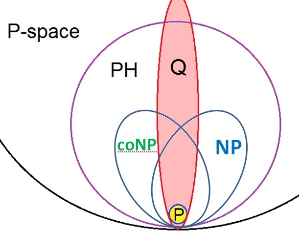
Figure 1. The (conjectured) view of some main computational complexity classes. The red ellipse represents efficient quantum algorithms.

Computational complexity is the theory of efficient computations, where “efficient” is an asymptotic notion referring to situations where the number of computation steps (“time”) is at most a polynomial in the number of input bits. For modern books on computational complexity, the reader is referred to Goldreich [23, 22] and Arora and Barak [9].

The complexity class P is the class of algorithms that can be performed using a polynomial number of steps in the size of the input. The complexity class NP refers to non-deterministic polynomial time. Roughly speaking, it refers to questions where we can provably perform the task in a polynomial number of operations in the input size, provided we are given a certain polynomial-size “hint” of the solution. An algorithmic task $A$ is NP-hard if a subroutine for solving $A$ allows solving any problem in NP in a polynomial number of steps. An NP-complete problem is an NP-hard problem in NP. Examples of NP-complete problems are: to decide if a graph has a Hamiltonian cycle, or to decide if a Boolean formula has a satisfying assignment. A problem is in coNP if its complement is in NP. For example, to decide if a graph does not have a Hamiltonian cycle is in coNP.

A useful analog is to think about the gap between NP and P as similar to the gap between finding a proof of a theorem and verifying that a given proof of the theorem is correct. P, NP, and coNP are three of the lowest computational complexity classes in the polynomial hierarchy PH, which is a countable sequence of such classes, and there is a rich theory of complexity classes beyond PH.

There are intermediate problems between P and NP. Factoring an $n$-digit integer is not known to be in P, as the best algorithms are exponential in the cube root of the number of digits. Factoring is in NP, but it is unlikely that factoring is NP-complete. Shor’s famous algorithm shows that quantum computers can factor $n$-digit integers efficiently – in $\sim n^{2}$ steps! Quantum computers are not known to be able to solve NP-complete problems efficiently, and there are good reasons to think that they cannot. However, quantum computers can efficiently perform certain computational tasks beyond NP. The class of decision problems (algorithmic tasks with a yes/no answer) that quantum computers can efficiently solve is denoted by BQP.

Two comments: first, our understanding of the world of computational complexity depends on a whole array of conjectures: NP $\neq$ P is the most famous one, and a stronger conjecture asserts that PH does not collapse, namely, that there is a strict inclusion between the computational complexity classes defining the polynomial hierarchy. Second, computational complexity insights, while asymptotic, strongly apply to finite and small algorithmic tasks. The following example will be important for our analysis: recall that the Ramsey number $R(n,n)$ is the smallest $m$ such that for every coloring of the edges of a complete graph on $m$ vertices with two colors, there is a complete graph on $n$ vertices all of whose edges are colored with the same color. Paul Erdős famously claimed that finding the value of the Ramsey function $R(n,n)$ for $n=6$ is well beyond mankind’s ability. This statement is supported by computational complexity insights that consider the difficulty of computations as $n\to\infty$, while not directly implied by them.

2. Noise

2.1. Noise and fault-tolerant computation

The main concern regarding the feasibility of quantum computers has always been that quantum systems are inherently noisy: we cannot accurately control them, and we cannot accurately describe them. The concern regarding noise in quantum systems as a major obstacle to quantum computers was put forward in the mid-90s by Landauer [42], Unruh [64], and others. To overcome this difficulty, a theory of quantum fault-tolerant computation based on quantum error-correcting codes was developed [55, 58, 56, 3, 39, 24, 41]; see also [47][Ch. 10]. Fault-tolerant computation refers to computation in the presence of errors. The basic idea is to represent (or “encode”) a single piece of information (a bit in the classical case or a qubit in the quantum case) by a large number of physical components so as to ensure that the computation is robust even if some of these physical components are faulty.

What is noise? Solutions of the Schrödinger equation (“quantum evolutions”) can be regarded as unitary processes on Hilbert spaces. Mathematically speaking, the study of noisy quantum systems is the study of pairs of Hilbert spaces $(H,H^{\prime})$, $H\subset H^{\prime}$, and a unitary process on the larger Hilbert space $H^{\prime}$. Noise refers to the general effect of neglecting degrees of freedom, namely, approximating the process on a large Hilbert space by a process on the small Hilbert space. For controlled quantum systems and, in particular, quantum computers, $H$ represents the controlled part of the system, and the large unitary process on $H^{\prime}$ represents, in addition to an “intended” controlled evolution on $H$, also the uncontrolled effects of the environment. The study of noise is relevant, not only to controlled quantum systems, but also to many other aspects of quantum physics.

A second, mathematically equivalent way to view noisy states and noisy evolutions is to stay with the original Hilbert space $H$, but to consider a mathematically larger class of states and operations. In this view, the state of a noisy qubit is described as a classical probability distribution on unit vectors of the associated Hilbert spaces. Such states are referred to as mixed states. It is convenient to think about the following form of noise, called depolarizing noise: in every computer cycle a qubit is not affected with probability $1-p$, and, with probability $p$, it turns into the maximal entropy mixed state, i.e., the average of all unit vectors in the associated Hilbert space. In this example, $p$ is the error rate, and, more generally, the error rate can be defined as the probability that a qubit is corrupted at a computation step conditioned on it having survived up to this step.

2.2. Two alternatives for noisy quantum systems

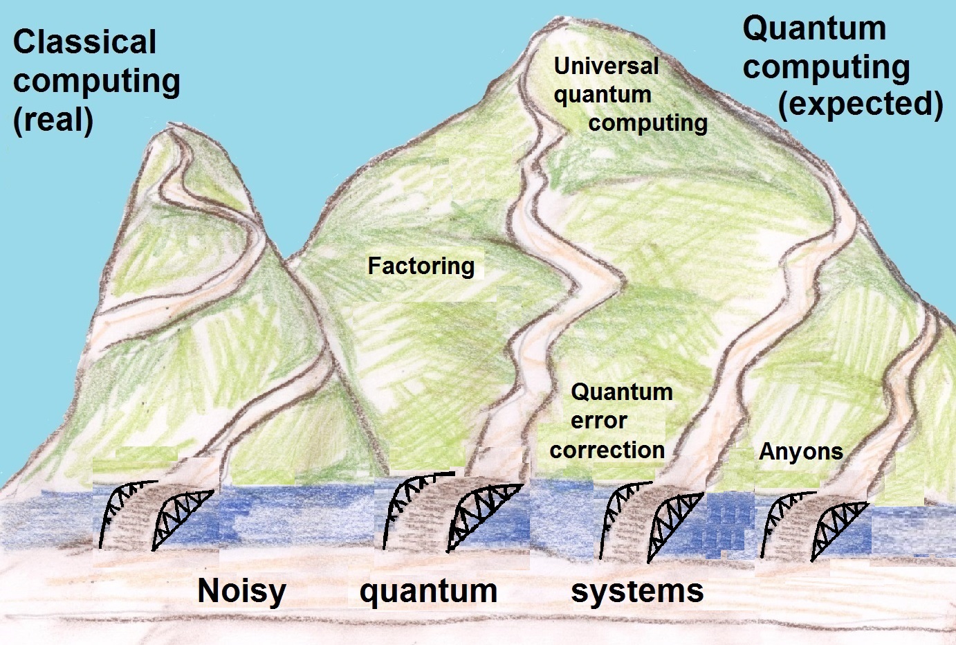
Figure 2. The optimistic hypothesis: Classical fault-tolerance mechanisms can be extended, via quantum error-correction, allowing robust quantum information and computationally superior quantum computation. Drawing by Neta Kalai.

The quantum computer puzzle is, in a nutshell, deciding between two hypotheses regarding properties of noisy quantum circuits, the optimistic hypothesis and the pessimistic hypothesis.

Optimistic hypothesis: It is possible to realize universal quantum circuits with a small bounded error level regardless of the number of qubits. The effort required to obtain a bounded error level for universal quantum circuits increases moderately with the number of qubits. Therefore, large-scale fault-tolerant quantum computers are possible.

Pessimistic hypothesis: The error rate in every realization of universal quantum circuits scales up (at least) linearly with the number of qubits. The effort required to obtain a bounded error level for any implementation of universal quantum circuits increases (at least) exponentially with the number of qubits. Thus, quantum computers are not possible.

Some explanations: for the optimistic hypothesis, we note that the main theorem of quantum fault-tolerance asserts that (under some natural conditions on the noise), if we can realize universal quantum circuits with a sufficiently small error rate (where the threshold is roughly between 0.001 and 0.01,) then quantum fault-tolerance and hence universal quantum computing are possible. For the pessimistic hypothesis, when we say that the rate of noise per qubit scales up linearly with the number of qubits we mean that when we double the number of qubits in the circuit the probability for a single qubit to be corrupted in a small time interval doubles. The pessimistic hypothesis does not require new modeling of the noise of universal quantum circuits, and it is just based on a different assumption on the rate of noise. However, for more general noisy quantum systems, it leads to interesting predictions and modeling, and may lead to useful computational tools. We emphasize that both hypotheses are assertions about physics (or physical reality), not about mathematics, and both of the hypotheses represent scenarios that are compatible with quantum mechanics.

The constants are important and the pessimistic view regarding quantum supremacy holds that every realization of universal quantum circuits will fail for a handful of qubits, long before any quantum supremacy effect is witnessed, and long before quantum fault-tolerance is possible. The failure to reach universal quantum circuits for a small number of qubits, and to manifest quantum supremacy for small quantum systems, is crucial for the pessimistic hypothesis, and Erdős’s statement about $R(6,6)$ is a good analogy for this expected behavior.

Both on the technical and conceptual levels we see here what we call a “wide-gap dichotomy.” On the technical level, we have a gap between small constant error rate per qubit for the optimistic view, and a linear increase of rate per qubit (in terms of the number of qubits in the circuit) on the pessimistic side. We also have a gap between the ability to achieve large-scale quantum computers on the optimistic side, and the failure of universal quantum circuits already for a handful of qubits on the pessimistic side. On the conceptual level, the optimistic hypothesis asserts that quantum mechanics allows superior computational powers, while the pessimistic hypothesis asserts that quantum systems without specific mechanisms for robust classical information that leads only to classical computing are actually computationally inferior. We will come back to both aspects of this wide-gap dichotomy.

2.3. Potential experimental support for quantum supremacy

A definite demonstration of quantum supremacy of controlled quantum systems, namely, building quantum systems that outperform, even for specific computational tasks, classical computers, or a definite demonstration of quantum error-correction, will falsify the pessimistic hypothesis and will lend strong support to the optimistic hypothesis. (The optimistic hypothesis will be completely verified with full-fledged universal quantum computers.) There are several ways people are planning, in the next few years, to demonstrate quantum supremacy or the feasibility of quantum fault-tolerance.

1. Attempts to create small universal quantum circuits with up to “a few tens of qubits.”

2. Attempts to create stable logical qubits based on surface codes.

3. Attempts to have BosonSampling for 10–50 bosons.

4. Attempts to create stable qubits based on anyonic states.

5. Attempts to demonstrate quantum speed-up based on quantum annealing.

Each of attempts (1)–(4) represents many different experimental directions carried out mainly in academic institutions (and research centers of large companies like IBM, Microsoft, and Google), while (5) represents an attempt by a commercial company: D-wave. There are many different avenues for realizing qubits, of which ion-trapped qubits and superconducting qubits are perhaps the leading ones, and there are several groups attempting to demonstrate stable logical qubits via quantum error-correction. Quantum supremacy via nonabelian anyons stands out as a very different direction based on exotic new phases of matter and very deep mathematical and physical issues. BosonSampling (see Section 3) stands out in the quest to demonstrate quantum supremacy for narrow physical systems without offering further practical fruits.

The pessimistic hypothesis predicts a decisive failure for all of these attempts to demonstrate quantum supremacy, or very stable logical qubits, and also that this failure will be witnessed for small systems. A reader may ask how the optimistic hypothesis can be falsified, beyond repeated failures to demonstrate universal quantum computers or partial steps toward them such as those listed above. My view is that the optimistic hypothesis could be largely falsified if we can understand the absence of quantum supremacy and quantum error-correction as a physical principle with prediction power that goes beyond these repeated failures – both in providing more detailed predictions about these failures themselves (such as scaling up of errors, correlations between errors, etc.) and in providing predictions about other natural quantum systems. Mathematical modeling of noisy quantum systems based on the pessimistic hypothesis is valuable, not only if it represents a general physical principle, but also if it represents temporary technological difficulties or if it applies to limited classes of quantum systems.

3. BosonSampling

Quantum computers would allow the creation of probability distributions that are beyond the reach of classical computers with access to random bits. This is manifested by “BosonSampling,” a class of probability distributions representing a collection of non-interacting bosons, that quantum computers can efficiently create. It is a restricted subset of distributions compared to the class of distributions that a universal quantum computer can produce, and it is not known if BosonSampling distributions can be used for efficient integer factoring or other “useful” algorithms. BosonSampling was introduced by Troyansky and Tishby in 1996 and was intensively studied by Aaronson and Arkhipov [2], who offered it as a quick path for experimentally showing that quantum supremacy is a real phenomenon.

Given an $n$ by $n$ matrix $A$, let $det(A)$ denote the determinant of $A$, and $per(A)$ denote the permanent of $A$. Thus $det(A)=\sum_{\pi\in S_{n}}sgn(\pi)\prod_{i=1}^{n}a_{i\pi(i)}$, and $per(A)=\sum_{\pi\in S_{n}}\prod_{i=1}^{n}a_{i\pi(i)}$. Let $M$ be a complex $n\times m$ matrix, $m\geq n$. Consider all ${m}\choose{n}$ subsets $S$ of $n$ columns, and for every subset consider the corresponding $n\times n$ submatrix $A$. The algorithmic task of sampling subsets $S$ of columns according to $|det(M^{\prime})|^{2}$ is called FermionSampling. Next consider all ${m+n-1}\choose{n}$ sub-multisets $S$ of $n$ columns (namely, allow columns to repeat), and for every sub-multiset $S$ consider the corresponding $n\times n$ submatrix $A$ (with column $i$ repeating $r_{i}$ times). BosonSampling is the algorithmic task of sampling those multisets $S$ according to $|per(A)|^{2}/(r_{1}!r_{2}!\cdots r_{n}!)$. Note that the algorithmic task for BosonSampling and FermionSampling is to sample according to a specified probability distribution. This is not a decision problem, where the algorithmic task is to provide a yes/no answer.

Let us demonstrate these notions by an example for $n=2$ and $m=3$. The input is a $2\times 3$ matrix:

$$\left(\begin{array}[]{ccc}1/\sqrt{3}&i/\sqrt{3}&1/\sqrt{3}\\ 0&1/\sqrt{2}&i/\sqrt{2}\end{array}\right)$$

The output for FermionSampling is a probability distribution on subsets of two columns, with probabilities given according to absolute values of the square of determinants. Here we have probability $1/6$ to columns $\{1,2\}$, probability $1/6$ to columns $\{1,3\}$, and probability $4/6$ to columns $\{2,3\}$. The output for BosonSampling is a probability distribution according to absolute values of the square of permanents of sub-multisets of two columns. Here, the probabilities are: $\{1,1\}\to 0$; $\{1,2\}\to 1/6$; $\{1,3\}\to 1/6$; $\{2,2\}\to 2/6$; $\{2,3\}\to 0$; $\{3,3\}\to 2/6$.

FermionSampling describes the state of $n$ non-interacting fermions, where each individual fermion is described as a superposition of $m$ “modes.” BosonSampling describes the state of $n$ non-interacting fermions, where each individual fermion is described by $m$ modes. A few words about the physics: fermions and bosons are the main building blocks of nature. Fermions, such as electrons, quarks, protons, and neutrons, are particles characterized by Fermi–Dirac statistics. Bosons, such as photons, gluons, and the Higgs boson, are particles characterized by Bose–Einstein statistics.

Moving to computational complexity, we note that Gaussian elimination gives an efficient algorithm for computing determinants, but computing permanents is very hard: it represents a computational complexity class, called #P (in words, “number P” or “sharp P”), that extends beyond the entire polynomial hierarchy. It is commonly believed that even quantum computers cannot efficiently compute permanents. However, a quantum computer can efficiently create a bosonic (and a fermionic) state based on a matrix $M$, and therefore perform efficiently both BosonSampling and FermionSampling. A classical computer with access to random bits can sample FermionSampling efficiently, but, as proved by Aaronson and Arkhipov, a classical computer with access to random bits cannot perform BosonSampling unless the polynomial hierarchy collapses! (See [2, 14, 60].)

4. Predictions from the optimistic hypothesis

Barriers crossed

Quantum computers would dramatically change our reality.

1. A universal machine for creating quantum states and evolutions will be built.

2. Complicated evolutions and states with global interactions, markedly different from anything witnessed so far, will be created.

3. It will be possible to experimentally time-reverse every quantum evolution.

4. The noise will not respect symmetries of the state.

5. There will be fantastic computational complexity consequences.

6. Quantum computers will efficiently break most current public-key cryptosystems.

Items 1–4 represent a vastly different experimental reality than that of today, and items 5 and 6 represent a vastly different computational reality.

Magnitude of improvements

It is often claimed that quantum computers could perform in a few hours certain computations that take longer than the lifetime of the universe on a classical computer! Indeed, it is useful to examine not only things that were previously impossible and which are now made possible by a new technology, but also the improvement in terms of orders of magnitude for tasks that could have been achieved by the old technology. Quantum computers represent enormous, unprecedented, order-of-magnitude improvement of controlled physical phenomena as well as of algorithms. Nuclear weapons represent an improvement of 6–7 orders of magnitude over conventional ordinance: the first atomic bomb was a million times stronger than the most powerful (single) conventional bomb at the time. The telegraph could deliver a transatlantic message in a few seconds compared to the previous three-month period. This represents an (immense) improvement of 4–5 orders of magnitude. Memory and speed of computers were improved by 10–12 orders of magnitude over several decades. Breakthrough algorithms at the time of their discovery also represented practical improvements of no more than a few orders of magnitude. Yet implementing BosonSampling with a hundred bosons represents more than a hundred orders of magnitude of improvement compared to digital computers, and a similar story can be told about a large-scale quantum computer applying Shor’s algorithm.

Computations in quantum field theory

Quantum electrodynamics (QED) computations allow one to describe various physical quantities in terms of a power series

$$\sum c_{k}\alpha^{k},$$

where $c_{k}$ is the contribution of Feynman’s diagrams with $k$ loops, and $\alpha$ is the fine structure constant (around 1/137). Quantum computers will (likely) allow one to compute these terms and sums for large values of $k$ with hundreds of digits of accuracy, similar to computations of the digits of $e$ and $\pi$ on today’s computers, even in regimes where they have no physical meaning!

My interpretation

I regard the incredible consequences from the optimistic hypothesis as solid indications that quantum supremacy might be “too good to be true,” and that the pessimistic hypothesis would prevail. Quantum computers would change reality in unprecedented ways, both qualitatively and quantitatively, and it is easier to believe that we will witness substantial theoretical changes in modeling quantum noise than that we will witness such dramatic changes in reality itself.

5. BosonSampling meets reality

5.1. How does noisy BosonSampling behave?

BosonSampling and noisy BosonSampling (i.e., BosonSampling in the presence of noise) exhibit radically different behavior. BosonSampling is based on $n$ non-interacting indistinguishable bosons with $m$ modes. For noisy Boson Samplers these bosons will not be perfectly non-interacting (accounting for one form of noise) and will not be perfectly indistinguishable (accounting for another form of noise). The same is true if we replace bosons by fermions everywhere. The state of $n$ bosons with $m$ modes is represented by an algebraic variety of decomposable symmetric tensors of real dimension $2mn$ in a huge relevant Hilbert space of dimension $2m^{n}$. For the fermion case this manifold is simply the Grassmanian. The study of noisy BosonSampling in [36] is based on a general framework for the study of noise and sensitivity to noise via Fourier expansion that was introduced by Benjamini, Kalai, and Schramm [11]; see also [20].

We have already discussed the rich theory of computational complexity classes beyond P, and there is also a rich theory below P. One very low-level complexity class consists of computational tasks that can be carried out by bounded-depth polynomial-size circuits. In this model the number of gates is, as before, at most polynomial in the input side, but an additional severe restriction is that the entire computation is carried out in a bounded number of rounds. Bounded-depth polynomial-size circuits cannot even compute or approximate the parity of $n$ bits, but they can approximate real functions described by bounded-degree polynomials and can sample approximately according to probability distributions described by real polynomials of bounded degree.

Theorem 1 (Kalai and Kindler [36]).

When the noise level is constant, BosonSampling distributions are well approximated by their low-degree Fourier–Hermite expansion. Consequently, noisy BosonSampling can be approximated by bounded-depth polynomial-size circuits.

It is reasonable to assume that for all proposed implementations of BosonSampling the noise level is at least a constant, and therefore, an experimental realization of BosonSampling represents, asymptotically, bounded-depth computation. The next theorem shows that implementation of BosonSampling will actually require pushing down the noise level to below $1/n$.

Theorem 2 (Kalai and Kindler [36]).

When the noise level is $\omega(1/n)$, and $m\gg n^{2}$, BosonSampling is very sensitive to noise with a vanishing correlation between the noisy distribution and the ideal distribution.

Theorems 1 and 2 give evidence against expectations of demonstrating “quantum supremacy” via BosonSampling: experimental BosonSampling represents an extremely low-level computation, and there is no precedence for a “bounded-depth machine” or a “bounded-depth algorithm” that gives a practical advantage, even for small input size, over the full power of classical computers, not to mention some superior powers.

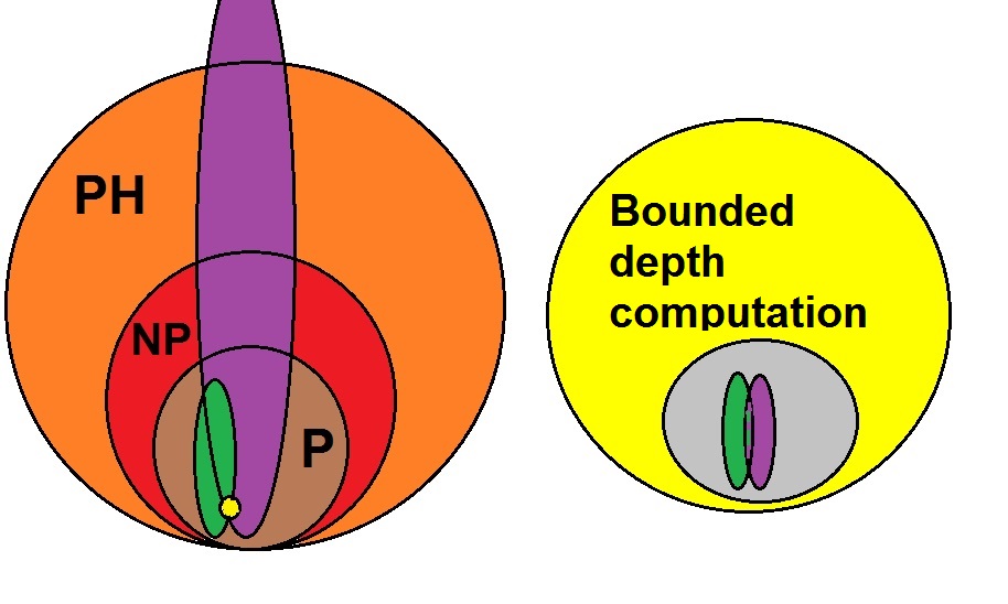
Figure 3. The huge computational gap (left) between BosonSampling (purple) and FermionSampling (green) vanishes in the noisy versions (right).

5.2. Bounded-degree polynomials

The class of probability distributions that can be approximated by low-degree polynomials represents a severe restriction below bounded-depth computation. The description of noisy BosonSampling with low bounded-degree polynomials is likely to extend to small noisy quantum circuits and other similar quantum systems and this would support the pessimistic hypothesis. This description is relevant to important general computational aspects of quantum systems in nature, to which we now turn.

Why is robust classical information possible?

The ability to approximate low-degree polynomials still supports robust classical information. The (“Majority”) Boolean function $f(x_{1},x_{2},\dots,x_{n})=sgn(x_{1}+x_{2}+\cdots+x_{n})$ allows for very robust bits based on a large number of noisy bits and admits excellent low-degree approximations. Quantum error-correction is also based on encoding a single qubit as a function $f(q_{1},q_{2}\dots,q_{n})$ of many qubits, and also for quantum codes, the quality of the encoded qubit grows with the number of qubits used for the encoding. But for quantum error-correcting codes, implementation with bounded-degree polynomial approximations (or even with law-depth computation) is not available, and I conjecture that no such implementation exists. This would support the insight that quantum mechanics is limiting the information one can extract from a physical system in the absence of mechanisms leading to robust classical information.

Why can we learn the laws of physics from experiments?

We talked about how hard it is to compute a known function. When we need to learn an unknown function we find ourselves in the realm of computational learning theory, a central area in the theory of computing with strong relations to artificial intelligence and to statistics [38, 53]. Learning the parameters of a process from examples can be computationally intractable, even if the process belongs to a low-level computational task. Learning even a function described by a depth-two Boolean circuit of polynomial size does not admit an efficient algorithm. Daniely, Linial, and Shalev-Shwartz [16] showed (under certain computational complexity assumptions) that general functions in ${\bf AC}^{\bf 0}$ (even of depth two) cannot be efficiently learned; namely, there is no efficient algorithm for learning the function by observing a small number of random examples. However, the approximate value of a low-degree polynomial can efficiently be learned from examples. This offers a theoretical explanation for our ability to understand natural processes and the parameters defining them.

Reaching ground states

Reaching ground states is computationally hard (NP-hard) even for classical systems, and for quantum systems it is even harder. So how does nature reach ground states so often? The common answer relies on two ingredients: the first is that physical systems operate in positive temperature rather than zero temperature, and the second is that nature often reaches meta-stable states rather than ground states. However, these explanations are incomplete: we have good theoretical reasons to think that, for general processes in positive temperature, reaching meta-stable states is computationally intractable as well. First, for general quantum or classical systems, reaching a meta-stable state can be just as computationally hard as reaching a ground state. Second, one of the biggest breakthroughs in computational complexity, the “PCP-theorem” (in physics disguise), asserts that positive temperature offers no computational complexity relief for general (classical) systems. Dealing with quantum evolutions and states approximated by low-degree polynomials may support the phenomenon of easily reached ground states.

6. Predictions from the pessimistic hypothesis

Under the pessimistic hypothesis, universal quantum devices are unavailable, and we need to devise a specific device in order to implement a specific quantum evolution. A sufficiently detailed modeling of the device will lead to a familiar detailed Hamiltonian modeling of the quantum process that also takes into account the environment and various forms of noise. Our goal is different: we want to draw from the pessimistic hypothesis predictions on noisy quantum circuits (and, at a later stage, on more general noisy quantum processes) that are common to all devices implementing the circuit (process).

The basic premises for studying noisy quantum evolutions when the specific quantum devices are not specified are as follows: first, modeling is implicit; namely, it is given in terms of conditions that the noisy process must satisfy. Second, there are systematic relations between the noise and the entire quantum evolution and also between the target state and the noise.

In this section we assume the pessimistic hypothesis, but we note that the previous section proposes the following picture in support of the pessimistic hypothesis: evolutions and states of quantum devices in the small scale are described by low-degree polynomials. This allows, for a larger scale, the creation of robust classical information and computation, but does not provide the necessary starting point for quantum fault-tolerance or for any manifestation of quantum supremacy.

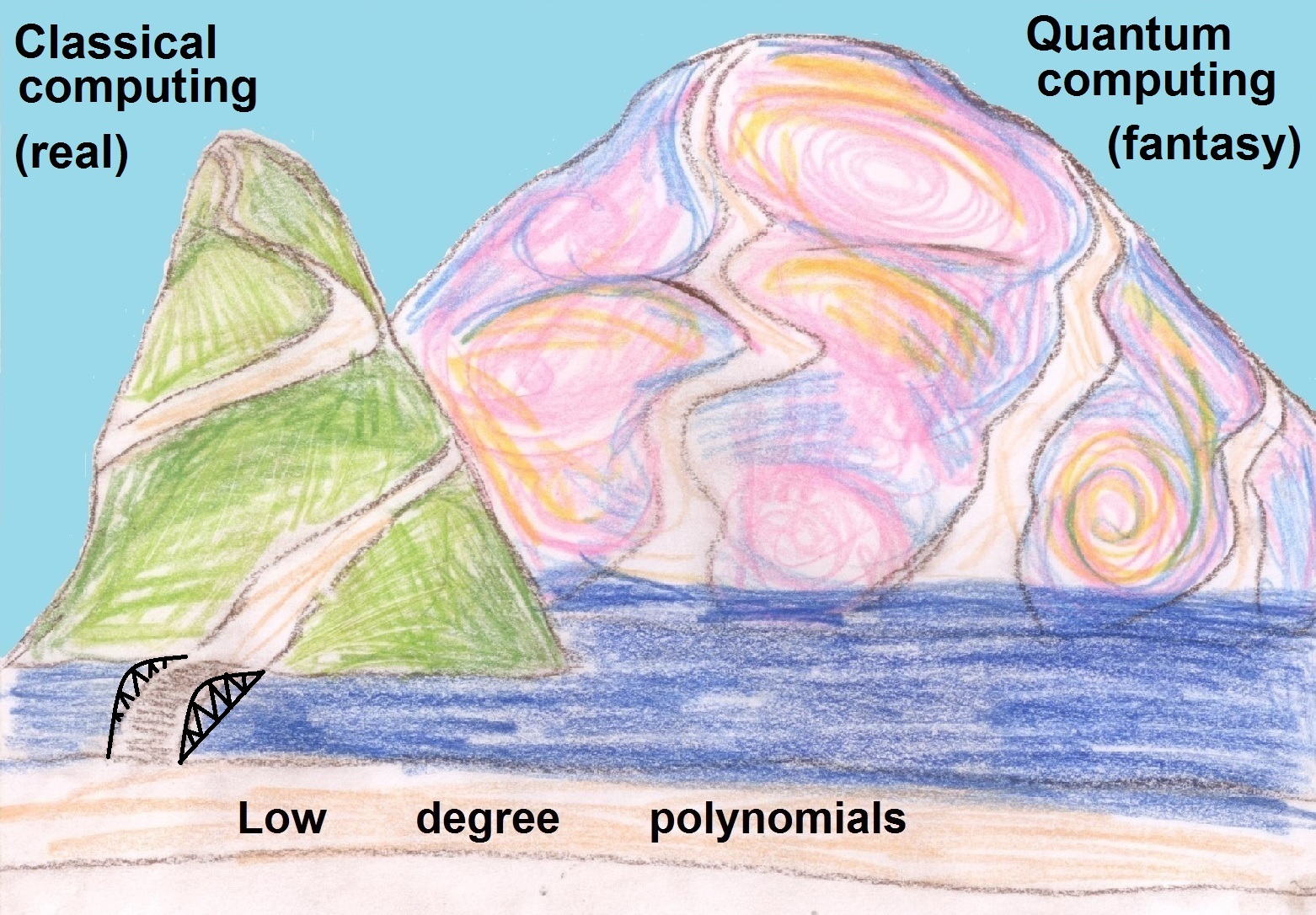
Figure 4. The pessimistic hypothesis: Noisy quantum evolutions, described by low-degree polynomials, allow, via the mechanisms of averaging/repetition, robust classical information and computation, but do not allow reaching the starting points for quantum supremacy and quantum fault-tolerance. Drawing by Neta Kalai.

6.1. No quantum fault-tolerance: Its simplest manifestation

Entanglement and cat states

Entanglement is a name for quantum correlation, and it is an important feature of quantum physics and a crucial ingredient of quantum computation. A cat state of the form ${\frac{1}{\sqrt{2}}}\left|00\right\rangle+{\frac{1}{\sqrt{2}}}\left|11\right\rangle$ represents the simplest form of entanglement between two qubits. Let me elaborate: the Hilbert space $H$ representing the states of a single qubit is two-dimensional. We denote by $\left|0\right\rangle$ and $\left|1\right\rangle$ the two vectors of a basis for $H$. A pure state of a qubit is a superposition of basis vectors of the form $a\left|0\right\rangle+b\left|1\right\rangle$, where $a,b$ are complex and $|a|^{2}+|b|^{2}=1$. Two qubits are represented by a tensor product $H\otimes H$ and we denote $\left|00\right\rangle=\left|0\right\rangle\otimes\left|0\right\rangle$, and $\left|11\right\rangle=\left|1\right\rangle\otimes\left|1\right\rangle$. A superposition of two vectors can be thought of as a quantum analog of a coin toss in classical probability. The superposition ${\frac{1}{\sqrt{2}}}\left|0\right\rangle+{\frac{1}{\sqrt{2}}}\left|1\right\rangle$ is a quantum analog of a coin toss giving head with probability 1/2 and tail with probability 1/2, and the superposition ${\frac{1}{\sqrt{2}}}\left|00\right\rangle+{\frac{1}{\sqrt{2}}}\left|11\right\rangle$ is a quantum analog of correlated coin tosses, i.e., two heads with probability 1/2, and two tails with probability 1/2. The name “cat state” refers, of course, to Schrödinger’s cat.

Noisy cats

The following prediction regarding noisy entangled pairs of qubits (or “noisy cats”) is perhaps the simplest prediction on noisy quantum circuits under the pessimistic hypothesis.

Prediction 1: Two-qubits behavior. Any implementation of quantum circuits is subject to noise, for which errors for a pair of entangled qubits will have substantial positive correlation.

Prediction 1, which we will refer to as the “noisy cat prediction,” gives a very basic difference between the optimistic and pessimistic hypotheses. Under the optimistic hypothesis, gated qubits will manifest correlated noise, but when quantum fault-tolerance is in place, such correlations will be diminished for most pairs of qubits. Under the pessimistic hypothesis quantum fault-tolerance is not possible, and without it there is no mechanism to remove correlated noise for entangled qubits. Note that the condition on noise for a pair of entangled qubits is implicit as it depends on the unknown process and unknown device leading to the entanglement.

Further simple manifestations of the failure of quantum fault-tolerance

Prediction 2: Error synchronization. For complicated (very entangled) target states, highly synchronized errors will occur.

Error synchronization refers to a substantial probability that a large number of qubits, much beyond the average rate of noise, are corrupted. Under the optimistic hypothesis error synchronization is an extremely rare event.

Prediction 3: Error rate. For complicated evolutions, and for evolutions approximating complicated states, the error rate, in terms of qubit errors, scales up linearly with the number of qubits.

The three predictions 1–3 are related. Under natural assumptions, the noisy cat prediction implies error synchronization for quantum states of the kind involved in quantum error-correction and quantum algorithms. Roughly speaking, the noisy cat prediction implies positive correlation between errors for every pair of qubits, and this implies a substantial probability for the event that a large fraction of qubits (well above the average rate of errors) will be corrupted at the same computer cycle. Error synchronization also implies, again under some natural assumptions, that error rate in terms of qubit errors is at least linear in the number of qubits. Thus, the pessimistic hypothesis itself can be justified from the noisy cat prediction together with natural assumptions on the rate of noise. Moreover, this also explains the wide-gap dichotomy in terms of qubit errors.

The optimistic hypothesis allows creating via quantum error-correction very stable “logical” qubits based on stable raw physical qubits.

Prediction 4: No logical qubits. Logical qubits cannot be substantially more stable than the raw qubits used to construct them.

6.2. A more formal description of the noisy cat condition

Given two qubits $q_{1},q_{2}$ in pure joint state $\rho$ the entropy of one of the qubits is a standard measure of entanglement that we denote by $Ent(\rho:q_{1},q_{2})$. We will consider depolarizing noise described by a $2\times 2$ matrix $(p_{i,j})$ describing the probabilities of none, only the first, only the second, and both qubits being corrupted. Let $E_{i},i=1,2$ be the event that the $i$th qubit was corrupted and let $r_{i}$ be the probability of $E_{i}$ and $cor(E_{1},E_{2})$ be the correlation between the events $E_{1}$ and $E_{2}$.

The noisy cat prediction asserts that any realization of a quantum circuit that approximates the pure state $\rho$ is subject to depolarizing noise with

$$cor(E_{1},E_{2})\geq K(r_{1},r_{2})\cdot Ent(\rho:q_{1},q_{2}).$$

Here, $K(x,y)$ is a function of $x$ and $y$ so that $K(x,y)/\min(x,y)^{2}\gg 1$ when $x$ and $y$ are positive and small.

A stronger form of the prediction applies to the emergent entanglement of a pair of qubits, namely, entanglement after some other qubits are measured (separately). The emergent entanglement of pairs of qubits is large both for quantum error-correcting codes needed for quantum fault-tolerance and quantum algorithms. The strong form of the prediction will imply substantial correlation of the noise between every pair of qubits. This implies error synchronization for quantum states of the kind involved in quantum error-correction and quantum algorithms. Assuming further that rate in terms of trace distance is constant for short time intervals implies that error rate in terms of qubit errors is at least linear in the number of qubits. This, in brief, is the reason for the wide-gap dichotomy between the optimistic and pessimistic hypotheses in terms of qubit errors. It is natural to assume that noise in terms of trace distance, (namely, bounded variation distance between probability distributions) is, for short time intervals, constant, because trace distance is invariant under unitary transformations. For more details see [33].

A few comments: first, to deal with noise it is very important to understand general sources and forms of noise, but for showing that noise cannot be dealt with, we can safely assume that depolarizing noise is present and restrict the discussion to depolarizing noise. Generally speaking, in this section we present predictions about noise when the system approximates well some ideal noiseless quantum state or evolution. Additional forms of noise may also be present. We don’t expect that (in practice) additional forms of noise will heal the damaging effects of our predicted noise. (This is theoretically possible [12].) Second, regardless of the possibility of quantum fault-tolerance we can expect our predictions to apply to any implementation of small quantum computers. Third, we note that arbitrary forms of correlation with a small error rate (in terms of qubit errors) still likely support log-depth quantum computation (hence Shor’s factoring) [32]. However, as discussed above, under natural assumptions, strong forms of correlation imply increased error rate in terms of qubit errors and vice versa.

6.3. No quantum fault-tolerance: its most general manifestation

We can go to the other extreme and try to examine consequences of the pessimistic hypothesis for the most general quantum evolutions. We start with a prediction related to the discussion in Section 5.

Prediction 5: Bounded-depth and bounded-degree approximations. Quantum states achievable by any implementation of quantum circuits are limited by bounded-depth polynomial-size quantum computation. Even stronger: low-entropy quantum states in nature admit approximations by bounded-degree polynomials.

The next items go beyond the quantum circuit model and do not assume that the Hilbert space for our quantum evolution has a tensor product structure.

Prediction 6: Time smoothing. Quantum evolutions are subject to noise with a substantial correlation with time-smoothed evolutions.

Time-smoothed evolutions form an interesting restricted class of noisy quantum evolutions aimed for modeling evolutions under the pessimistic hypothesis when fault-tolerance is unavailable to suppress noise propagation. The basic example for time-smoothing is the following: start with an ideal quantum evolution given by a sequence of $T$ unitary operators, where $U_{t}$ denotes the unitary operator for the $t$-th step, $t=1,2,\dots T$. For $s<t$ we denote $U_{s,t}=\prod_{i=s}^{t-1}U_{i}$ and let $U_{s,s}=I$ and $U_{t,s}=U^{-1}_{s,t}.$ The next step is to add noise in a completely standard way: consider a noise operation $E_{t}$ for the $t$-th step. We can think about the case where the unitary evolution is a quantum computing process and $E_{t}$ represents a depolarizing noise with a fixed rate acting independently on the qubits. And finally, replace $E_{t}$ with a new noise operation $E^{\prime}_{t}$ defined as the average

(6.1) $$E^{\prime}_{t}=\frac{1}{T}\cdot\sum_{s=1}^{T}U_{s,t}E_{s}U^{-1}_{s,t}.$$

Prediction 7: Rate. For a noisy quantum system a lower bound for the rate of noise in a time interval is a measure of non-commutativity for the projections in the algebra of unitary operators in that interval.

Predictions 6 and 7 are implicit and describe systematic relations between the noise and the evolution. We expect that time-smoothing will suppress high terms for some Fourier-like expansion, thus relating Predictions 6 and 5. We also note that Prediction 7 resembles the picture of the “unsharpness principle” from symplectic geometry and quantization [49].

6.4. Locality, space, and time

The decision between the optimistic and pessimistic hypotheses, is, to a large extent, a question about modeling locality in quantum physics. Modeling natural quantum evolutions by quantum computers represents the important physical principle of “locality”: quantum interactions are limited to a few particles. The quantum circuit model enforces local rules on quantum evolutions and still allows the creation of very non-local quantum states. This remains true for noisy quantum circuits under the optimistic hypothesis. The pessimistic hypothesis suggests that quantum supremacy is an artifact of incorrect modeling of locality. We expect modeling based on the pessimistic hypothesis, which relates the laws of the “noise” to the laws of the “signal,” to force a strong form of locality for both.

We can even propose that spacetime itself emerges from the absence of quantum fault-tolerance. It is a familiar idea that since (noiseless) quantum systems are time-reversible, time emerges from quantum noise (decoherence). However, also in the presence of noise, with quantum fault-tolerance, every quantum evolution that can experimentally be created can be time-reversed and, in fact, we can time-permute the sequence of unitary operators describing the evolution in an arbitrary way. It is therefore both quantum noise and the absence of quantum fault-tolerance that enable an arrow of time.

Next, we note that with quantum computers one can emulate a quantum evolution on an arbitrary geometry. For example, a complicated quantum evolution representing the dynamics of a four-dimensional lattice model could be emulated on a one-dimensional chain of qubits. This would be vastly different from today’s experimental quantum physics, and it is also in tension with insights from physics, where witnessing different geometries supporting the same physics is rare and important. Since a universal quantum computer allows the breaking of the connection between physics and geometry, it is noise and the absence of quantum fault-tolerance that distinguish physical processes based on different geometries and enable geometry to emerge from physics.

6.5. Classical simulations of quantum systems

Prediction 8: Classical simulations of quantum processes. Computations in quantum physics can, in principle, be simulated efficiently on a digital computer.

This bold prediction from the pessimistic hypothesis could lead to specific models and computational tools. There are some caveats: heavy computations may be required (1) for quantum processes that are not realistic to start with, (2) for a model in quantum physics representing a physical process that depends on many more parameters than those represented by the input size, (3) for simulating processes that require knowing internal parameters of the process that are not available to us (but are available to nature), and (4) when we simply do not know the correct model or relevant computational tool.

7. Additional predictions from the pessimistic hypothesis

We describe here a few further predictions from the pessimistic hypothesis. There are classes of quantum states that require deep (namely, of large depth) quantum computing and are thus unattainable under the pessimistic hypothesis. Since mixed states have multiple representations in terms of pure states, within a symmetry class of quantum states (or a class described by other terms), it is possible that low-entropy states will not be supported by low-degree polynomials and will thus be infeasible, while higher-entropy states in the class will admit low-depth/low-degree description and will actually be feasible. This leads to:

Prediction 9: Cooling. Within a symmetry class of quantum states (or for classes of states defined in a different way), the bounded-depth/low-degree polynomial requirement provides an absolute lower bound for cooling.

Of course, reaching low-temperature states in a certain class of quantum states may reflect a harder engineering task under both hypotheses. Under the pessimistic hypothesis, however, we may actually witness some threshold (depending on the class) that we cannot cross as the engineering difficulty explodes. This remark applies to a few of the other predictions below. (Here, the explosion of difficulty of computing Ramsey numbers is a good “role model.”)

We outline an important special case. Anyonic states [46, 40] are of special interest, both on their own and as a potential avenue for quantum computing.

Prediction 10: Anyons. Stable anyonic qubits cannot be constructed.

Next, under the pessimistic hypothesis the noisy process leading to a quantum state with a certain symmetry will introduce noise obeying the same symmetry. (Of course, other forms of noise may also be present.)

Prediction 11: Symmetry. Noisy quantum states and evolutions are subject to noise that respects their symmetries.

An interesting example is that of Bose–Einstein condensation. For a Bose–Einstein state on a bunch of atoms, one type of noise corresponds to independent noise for the individual atoms. (This type of noise is similar to standard noise for quantum circuits.) Another type of noise represents fluctuations of the collective Bose–Einstein state itself. This is the noise that respects the internal symmetries of the state and we expect that under the pessimistic hypothesis such a form of noise must always be present.

Our next prediction challenges one of the consequences of the general Hamiltonian models allowing quantum fault-tolerance [59, 8, 52]. These models allow some noise correlation over time and space but they are characterized by the fact that the error fluctuations are sub-Gaussian. Namely, when there are $N$ qubits the standard deviation for the number of qubit errors behaves like $\sqrt{N}$ and the probability of more than $t\sqrt{N}$ errors decays as it does for Gaussian distribution. These properties are not necessary for quantum fault-tolerance but they are shared by the rather general Hamiltonian models for noisy quantum computers that allow quantum fault-tolerance.

Prediction 12: Fluctuation. Fluctuations in the rate of noise for interacting $N$-element systems (even in cases where interactions are weak and unintended) scale like $N$ and not like $\sqrt{N}$.

Our prediction about fluctuation of noise for interacting systems can be tested in a variety of places. For example, we can consider a single superconducting qubit as a quantum device based on a large number of microscopic elements and study how stable its instabilities are. Prediction 4.4 can also be tested on digital memories (where interactions are unintended). Systems for highly precise physical clocks are characterized by having a huge number $N$ of elements with extremely weak interactions. We still expect (and this may be supported by current knowledge) that in addition to $\sqrt{N}$-fluctuations there will be also some $\epsilon N$-fluctuations. The relation between the level of interaction and $\epsilon$ can be useful for making quantitative versions of our predictions on correlated noise for systems with interaction. Another well-studied issue that might be relevant here is the statistical behavior of decay-time of particles and various other quantum systems.

Prediction 13: Teleportation. Teleportation of complicated quantum states is not possible.

Teleportation is an important, well-studied, and experimentally tested quantum physics phenomenon. Under the pessimistic hypothesis there are quantum states described efficiently by quantum circuits that are beyond reach. For complicated quantum states that are realistic, since teleportation itself involves additional noise and would require quantum fault-tolerance, teleportation need not be possible. With the absence of quantum fault-tolerance, quantum teleportation of complex quantum systems may well be impossible.

Again, an example based on non-interacting bosons is in order. Consider a photonic implementation of BosonSampling. We expect that already for fairly low values of $n$ we will not be able to reach with good accuracy BosonSampling states based on random Gaussian $n\times 2n$ matrix for $n$ photons and $2n$ modes. Let’s suppose that the threshold will be $n=8$. The threshold may well go down to $n=4$ or $n=5$ if we pose a more difficult task of achieving such a goal and then teleporting our $n$ photons to $n$ different locations 100 miles apart.

Prediction 14: Reversing the arrow of time. There are quantum evolutions that can be demonstrated but cannot be time-reversed.

Under the pessimistic hypothesis there are quantum evolutions (described, say, by quantum circuits) that cannot be realized (approximately). We can expect that the class of realistic noisy quantum evolutions is not invariant under time-reversing, and that there are easy-to-implement evolutions whose time-reversed versions are infeasible. (Of course, we do not restrict ourselves to actual physical implementations of quantum circuits via qubits and gates.) Thus, it may well be the case that we cannot, in principle, turn an omelet into an egg. (But simpler examples would certainly be desirable.) By a similar token:

Figure 5. Cats with unusual geometry in paintings by Gianantonio Muratori (in Braque’s style, left) and by Louis Wain (right)

Prediction 15: Geometry. Quantum states and evolutions reveal some information on the geometry of (all) their physical realizations.

Prediction 16: Superposition. There are pairs of quantum states/evolutions that can be created separately but cannot be superposed.

Quantum noise and the absence of quantum fault-tolerance leads also to:

Prediction 17: Predictions. Complex quantum systems cannot be predicted.

Consider again an experiment aimed at approximating the quantum state of BosonSampling based on a random Gaussian matrix, with $n$ bosons and $2n$ modes. In view of [36] (see, Section 5), we expect that the engineering effort required for a noise level below $1/n$, will explodes already for a small value of $n$. (Say, $n=8$.) On the other hand, for somewhat larger values of $n$ (say, $n=12$) when the noise level is above $1/n$, the experimental outcomes will not be robust. Noise sensitivity does not allow robust experimental outcomes because of the dependence of the state on an exponential number of parameters describing the actual noise [36][Sec. B.4]. Therefore, it will not be possible (in principle) to predict the outcome of the experiment, even in terms of a probability distribution.^,

As before, it will be desirable to find concrete, formal, and quantitative versions of all these predictions. We note also that it can be an interesting mathematical challenge to relate the different predictions based on the pessimistic hypothesis. One example would be to prove that noise preserves symmetry for noise described by time-smoothing.

7.1. Predictions for a living cat

Following the tradition of using cats for quantum thought experiments, consider an ordinary living cat. (An ordinary cat, not a Schrödinger cat.) All the difficulties predicted based on the pessimistic hypothesis for a handful of non-interacting photons positioned in interesting quantum states are expected to apply to the cat as well. Under the pessimistic hypothesis and the in-principle absence of quantum fault-tolerance, it will be impossible to teleport the cat, it will be impossible to reverse the life-evolution of the cat, it will not be possible to implement the cat at a very low temperature, or on a device with very different geometry, it will be impossible to superpose the life-evolutions of two distinct cats, and, finally, we predict that, even if we place the cat in an isolated and monitored environment, the life-evolution of this cat cannot be predicted.

8. Discussion

8.1. Noise and scalability

The emerging picture

Let me start by summarizing the picture drawn in Sections 5, 6, and 7. Standard noise models for evolutions and states of quantum devices in the small scale lead to a description by low-degree polynomials that manifests very low computational power that does not allow quantum fault-tolerance and quantum supremacy to emerge. This behavior in the small scale allows, for larger scales, the creation of robust classical information and computation (Section 5). The inability to reach the starting point for quantum fault-tolerance in the small scale has far-reaching consequences for the behavior of noisy quantum systems in the medium and large scale. In particular, it leads to novel implicit ways for modeling noise (Sections 6) that express the additional property of “no quantum fault-tolerance.”

The nature of noise

Some researchers regard noise solely as an engineering issue, and others even posit that noise does not have any objective meaning. I tend to disagree but, in any case, these views raise interesting conceptual issues and are related to the question of whether quantum supremacy is a real phenomenon.

The gap in intuitions regarding scaling

The pessimistic and optimistic hypotheses reflect different intuitions of the difficulties of scaling up systems. The optimistic hypothesis relies on the belief that scaling up an engineering device based on $n$ elements represents polylogarithmic or polynomial-scale difficulty rather than exponential difficulty. In view of the picture drawn in Section 5, the pessimistic hypothesis is based on the following alternative: scaling up an engineering device based on $n$ elements that perform asymptotically a task in a very low-level complexity class will fail well before the device demonstrates full classic computational powers or superior computational powers. Note that the pessimistic intuition about scaling is supported by computational complexity considerations applied (rather unusually) to small systems.

Modeling by quantum circuits

Under the pessimistic hypothesis, universal quantum circuits are beyond reach and they cannot be achieved even for a small number of qubits. But quantum circuits remain a powerful framework and model for quantum evolutions. Abstract quantum circuits are general enough to model processes in quantum physics (in fact, vastly more general), but note that we cannot take for granted that any realistic quantum process can be realized by a realistic implementation of a quantum circuit.

Computers and circuits

There are two slightly different ways to interpret “realizing universal quantum circuits” referred to in our hypotheses. Let us consider quantum circuits based on a fixed universal set of quantum gates. The simplest interpretation that we use in the paper is that we seek devices which realize arbitrary such circuits and we allow a special device for each circuit. The optimistic hypothesis asserts that with feasible engineering efforts every such circuit could be realized with a bounded and small error rate per qubit per computation step. The pessimistic hypothesis asserts that even for specific circuits needed for quantum algorithms, the error rate would scale up and the engineering effort required for keeping it small would thus explode. The optimistic view is actually slightly stronger: it asserts that one can build a universal controlled device, a quantum computer, that would allow to implement every quantum computational process, just like a digital computer can implement every Boolean computation.

How does the future evolution affect the present noise?

Under the pessimistic hypothesis, there is a systematic relation between the law for the noise at a given time and the entire evolution, including the future evolution. This is demonstrated by our smoothed formula (6.1). We can ask how can the current noise (or risk) depend on the future evolution. The answer is that it is not that the evolution in the future causes the behavior of the noise in the past, but rather that the noise in the past leads to constraints on possible evolutions in the future. Such dependence occurs also in classical systems. Without refueling capabilities, and without a very detailed description of the spacecraft, calculating the risk of space missions at take-off will strongly depend on the details of the full mission. (Such dependence can largely be be eliminated with refueling capabilities.) The pessimistic hypothesis implies that in the quantum setting such dependence cannot be eliminated.

Here is another example: suppose you are told that you need to undergo an operation at the age of fifty to avoid serious health problems in the following decade. This makes the risk at age fifty, conditioned on living to eighty, higher. Of course, in this scenario, it is not that living to eighty raises the risk at fifty, but rather that not taking the risky alternative at fifty makes it impossible to live to eighty.

8.2. Some further connections with physics, mathematics, and computation.

Quantum simulators, and proposals for quantum systems that cannot be simulated classically.

From time to time there are claims regarding quantum supremacy being manifested in some special-purpose quantum devices and, in particular, quantum simulators that simulate some quantum systems via quantum devices of a different nature. One such claim is outlined by a recent blog comment (Shtetl Optimized, September 2015) by Troyer: “The most convincing work so far might be [61] which looks at the dynamics of a correlated Bose gas. There the quantum simulation agrees with state of the art classical methods as long as they work, but the quantum simulation reaches longer times. The reason is a growing entanglement entropy which at some point causes the classical simulations to become unreliable. This is however one of the first demonstrations of a quantum simulator providing results that we don’t have a classical algorithm for.”

Like other supreme powers, quantum supremacy is appealing and has notable explanatory capability. I expect, however, that, in this case, the phenomenon of “growing entanglement entropy,” which causes classical simulations to become unreliable, amounts to the decay of some high-degree coefficients in a Fourier-like expansion, similar to the situation of noisy BosonSampling studied in [36], and that the classical simulator can be replaced by a better classical simulator representing low-level classical complexity for growing entropy.

Thermodynamics and other areas of physics

Properties of noise and the nature of approximations in quantum physics are very important in many areas of theoretical and experimental physics. Absence of quantum fault-tolerance seems especially relevant to the interface of thermodynamics and quantum physics. For example, the relations between the “signal” and “noise” in noise-modeling and predictions under the pessimistic hypothesis look similar to an important hypothesis/rule of Onsager from classical thermodynamics. We note that Alicki and several coauthors have over the years studied relations between quantum error-correction and thermodynamics (see, e.g.,[5]).

We briefly mentioned in Section 4 the relevance of quantum computing to computations in quantum field theory. “Noise” may well refer to the familiar phenomenon that for some scale, computations based on one theory (say QED computations) need to be corrected because of the effect of another theory (say, effects coming from the weak force). Our discussion here suggests that there could be systematic general rules for such corrections that have a bearing both on practical computations and on computational complexity issues.

Locality and entanglement

The pessimistic hypothesis excludes the ability to create highly entangled states from local operations (quantum computation processes). It does not exclude the possibility of “background” entangled systems that do not interact with our “local” physics. In fact, the same Hilbert space may admit different tensor product representations and hence different local structures, so that very mundane states for the one are highly entangled for the other. This possibility may represent real physical phenomena both under the pessimistic and optimistic hypotheses. (Of course, there could be “background” states that cannot be described by any local structure.)

There have been recent attempts to apply quantum information ideas and entanglement in particular to the study of quantum gravity and other basic topics in theoretical physics. Generally speaking, the pessimistic hypothesis is not in conflict with such ideas, and it may lead to interesting insights into them.

Classical physics, symplectic geometry, quantization, quantum noise, and the unsharpness principle

The unsharpness principle is a property of noisy quantum systems that can be proved for certain quantization of symplectic spaces. This is studied by Polterovich in [49] who relies on deep notions and results from symplectic geometry and follows, on the quantum side, some earlier works by Ozawa [48], and by Busch, Heinonen, and Lahti [15]. Here the notion of noise is different. The crucial distinction is between general positive operator-valued measures (POVMs) and vonNeumann observables, which are special cases of POVMs (also known as projector-valued POVMs). The unsharpness principle asserts that certain noisy quantum evolutions described by POVMs must be “far” from vonNeumann observables. The amount of unsharpness is bounded below by some non-commutativity measure. (This resembles our Prediction 7.) We note that the unsharpness principle depends on some notion of locality: it applies to systems based on “small” (displaceable) sets, where a set $X$ is displaceable if there is a Hamiltonian diffeomorphism of the entire underlying Hamiltonian manifold so that the image of $X$ is disjoint from $X$. It will be interesting to pursue further mathematical relations between the unsharpness principle, smoothed evolutions, and other issues related to quantum fault-tolerance.

The black hole firewall information paradox

According to the classical theory of black holes an object (which can be a photon, and is usually referred to as “Alice”) can pass through the event horizon of the black hole, never to return. But when you add quantum mechanics considerations (see, e.g., [27, 7]), you are driven to the conclusion that the event horizon itself represents singularity – the interior of the black hole does not exist. In other words, Alice will burn up passing through it. The sharply different view arising from QM is based on the fact that the same particle cannot be in entanglement with two different particles. It was raised in a work by Almheiri, Marolf, Polchinski, and Sully [7]. (There are other forms of the paradox. For example, there is an argument that Alice will eventually evaporate and all its quantum information will be lost, in contrast to the reversibility of quantum mechanics. Of course, since we lack a detailed theory for quantum gravity, there is something tentative/philosophical about the paradox and its proposed solutions.) It will be interesting to examine the relevance of the pessimistic hypothesis and absence of quantum fault tolerance to the paradox. Specifically, it will be interesting to study if cosmological reasoning related to the black hole firewall paradox leads to concrete estimates of the constants for Predictions 1 and 4. Hayden and Harlow [26] studied connections with quantum computation and argued that implementing the thought experiment that demonstrates the unexpected singularity at the event horizon is computationally intractable. (More precisely, verifying the expected outcome of the thought-experiment is intractable.) Maldacena and Susskind [44] offered a solution (based on what they call the ER=EPR principle). According to Susskind (private communication), for firewalls to arise requires sufficient quantum-computational power, rather than “ordinary interaction with the environment.” The pessimistic hypothesis provides a way to define “ordinary interaction with the environment,” and it asserts that no extraordinary interactions are at all possible.

More on permanents: From Polya to Barvinok

The huge computational gap between computing determinants and permanents makes an early appearance with the following problem proposed by Polya and solved by Szegö in 1913 ([45], Ch. 1.4): “Show that there is no linear transformation $T$ on the ($n^{2}$-dimensional) space of $n\times n$ matrices, $n\geq 3$, such that $per(M)=det(T(A))$.”

Approximating permanents of general real or complex matrices is #P-hard. But while approximating the value of permanents is hard in general, it is sometimes easy. An important result by Jerrum, Sinclair, and Vigoda [29] asserts that permanents of positive real matrices can be approximated in polynomial type up to a multiplicative factor $1+\epsilon$, for every $\epsilon>0$. Another important work on the computational complexity of approximating permanents is by Gurvits [25].

Barvinok [10] recently demonstrated remarkable results on approximating permanents. He showed that under certain constraints on the matrix’s entries, approximating the value of the permanent of an $n$ by $n$ matrix admits a quasi-polynomial time algorithm and, moreover, the value of the permanent can be well approximated by low- (logarithmic in $n$) degree polynomials. One example of such a constraint is when all entries are of the form $x+yi$, where $x\in[\delta,1]$, $\delta>0$, and $|y|\leq 0.5\delta^{3}$. Barvinok proved that if the permanent does not vanish in a certain region in the space of matrices then the value of the permanent is well approximated by low-degree polynomials well inside the region. It will be interesting to check if, for Barvinok’s good regions, BosonSampling is stable under noise and is practically feasible. Of special interest is the class of real matrices with entries between $\delta$ and 1.

FourierSampling and more on BosonSampling

Given a Boolean function $f$ that can be computed efficiently, a quantum computer can sample according to the Fourier coefficients of $f$ [57]. (A similar statement applies to functions defined on the integers that can be efficiently computed in terms of the number of digits.) This computational task, called FourierSampling, is crucial for many quantum algorithms, including Shor’s factoring. Similar computational results as mentioned for BosonSampling apply to FourierSampling, and approximately demonstrating FourierSampling for forty qubits or so is also regarded as a quick experimental path toward demonstrating quantum supremacy.

It is worth mentioning that the computational difficulty in demonstrating BosonSampling (and FourierSampling) goes even further than what we stated in Section 3. A classical (randomized) computer equipped with a subroutine that can perform an arbitrary task in the entire polynomial hierarchy cannot perform BosonSampling unless the polynomial hierarchy itself collapses [2]. It is even a plausible conjecture [36] that a classical (randomized) computer equipped with a subroutine that can perform an arbitrary task in BQP (or even QMA) cannot perform BosonSampling (and FourierSampling). If true, this would demonstrate a computational gap between quantum decision problems and quantum sampling problems.

Computational power of other classes of evolutions: Navier–Stokes computation

Quantum computing is an attempt to explore the computational power supported by quantum evolutions and quantum physics. One may well study computational aspects of other classes of evolutions. (See, e.g., [67].) Tao conjectures [62] that systems described by three-dimensional Navier–Stokes equations support fault-tolerance, and universal classical computation. This conjecture would imply finite-time blowup for those equations for certain initial conditions and thus disprove a major open problem in mathematics. Our discussion suggests various ways to express the negation of Tao’s conjecture, either as a mathematical alternative to Tao’s proposal or as a physical condition for “realistic” Navier–Stokes evolutions if Tao’s conjecture holds.

For demonstrating a property of “no computation” for a systems like those based on the 3D Navier–Stokes equation, we can try to derive or impose a “bounded degree” description for states and evolutions described by the system. (We will need also to study whether robust classical information via ”majority” is supported by the evolution.) Showing (or assuming) that the system is well approximated by a time-smoothed version may also be relevant. For Navier–Stokes evolutions as for other classes of evolutions, proving or imposing “no-computation” may also lead to additional interesting non-classical conserved quantities.

9. What is our computational world?

The remarkable progress witnessed during the past two decades in the field of experimental physics of controlled quantum systems places the decision between the pessimistic and optimistic hypotheses within reach. These two hypotheses reflect a vast difference in perspective regarding our computational world. Does the wealth of classical computations we witness in reality represent the full computational power that can be extracted from natural quantum physics processes, or is it only the tip of the iceberg of a supreme computational power used by nature and available to us?

Quantum computers represent a new possibility acquired through a beautiful interaction of many scientific disciplines. However unlikely it is and wherever it goes, this idea offers a terrific opportunity and may change a great deal. I expect that the pessimistic hypothesis will prevail, yielding important outcomes for physics, the theory of computing, and mathematics. Our journey through probability distributions described by low-degree polynomials, implicit modeling for noise, and error synchronization may provide some of the pieces needed for solving the quantum computer puzzle.

References

- [1] S. Aaronson, Multilinear formulas and skepticism of quantum computing. In STOC ’04: Proceedings of the thirty-sixth annual ACM symposium on Theory of computing, pp. 118–127. ACM Press, 2004.
- [2] S. Aaronson and A. Arkhipov, The computational complexity of linear optics, Theory of Computing 4 (2013), 143–252. arXiv:1011.3245
- [3] D. Aharonov and M. Ben-Or, Fault-tolerant quantum computation with constant error, in STOC ’97, ACM, New York, 1999, pp. 176–188.
- [4] R. Alicki, Quantum error correction fails for Hamiltonian models, 2004, quant-ph/0411008.
- [5] R. Alicki and M. Horodecki, Can one build a quantum hard drive? A no-go theorem for storing quantum information in equilibrium systems, quant-ph/0603260.
- [6] R, Alicki, Critique of fault-tolerant quantum information processing, in Quantum Error Correction, ed. D. A. Lidar and T. A. Brun, Cambridge University Press, 2013.
- [7] A. Almheiri, D. Marolf, J. Polchinski, and J. Sully, Black holes: complementarity or firewalls?, arXiv:1207.3123.
- [8] P. Aliferis, D. Gottesman, and J. Preskill, Quantum accuracy threshold for concatenated distance-3 codes, quant-ph/0504218.
- [9] S. Arora and B. Barak, Computational Complexity: Modern Approach, Cambridge University Press, 2009.
- [10] A. Barvinok, Approximating permanents and hafnians of positive matrices, arXiv:1601.07518
- [11] I. Benjamini, G. Kalai, and O. Schramm, Noise sensitivity of Boolean functions and applications to percolation, Publ. I.H.E.S. 90 (1999), 5–43.
- [12] M. Ben-Or, D. Gottesman, A. Hassidim, Quantum refrigerator, arXiv:1301.1995.
- [13] E. Bernstein and U. Vazirani, Quantum complexity theory, Siam J. Comp. 26 (1997), 1411–1473. (Earlier version, STOC, 1993.)
- [14] M. J. Bremner, R. Jozsa, D. J. Shepherd, Classical simulation of commuting quantum computations implies collapse of the polynomial hierarchy, Proc. Roy. Soc. A, 467(2011) ,459–472, 2011.
- [15] P. Busch, T. Heinonen, and P. Lahti, Noise and disturbance in quantum measurement, Phys. Lett. A 320 (2004), 261–270.
- [16] A. Daniely, N. Linial, and S. Shalev-Shwartz, Complexity-theoretic limitations on learning DNF’s, arXiv:1311.2272.
- [17] D. Deutsch, Quantum theory, the Church-Turing principle and the universal quantum computer, Proc. Roy. Soc. Lond. A 400 (1985), 96–117.
- [18] M. I. Dyakonov, Is fault-tolerant quantum computation really possible? in: Future Trends in Microelectronics. Up the Nano Creek, S. Luryi, J. Xu, and A. Zaslavsky (eds.), Wiley (2007), pp. 4–18.
- [19] R. P. Feynman, Simulating physics with computers, Int. J. Theor. Phys. 21 (1982), 467–488.
- [20] C. Garban and J. Steif, Noise Sensitivity of Boolean Functions and Percolation, Cambridge University Press, 2014.
- [21] O. Goldreich, On quantum computers, 2004, 2005, available on Goldreich’s homepage.
- [22] O. Goldreich, Computetional Complexity: A Conceptual Perspective, Cambridge University Press, 2008.
- [23] O. Goldreich, P, NP, and NP-Completeness: The Basics of Complexity Theory, Cambridge University Press, 2010.
- [24] D. Gottesman, Stamilizer codes and quantum error-correction, Ph. D. Thesis, Caltech, 1997.
- [25] L. Gurvits, On the complexity of mixed discriminants and related problems, Mathematical Foundations of Computer Science 2005, Lecture Notes in Computer Science, vol. 3618, Springer, Berlin, 2005, pp. 447–458.
- [26] D. Harlow and P. Hayden, Quantum Computation vs. Firewalls, arXiv:1301.4504.
- [27] D. Harlow, Jerusalem lectures on black holes and quantum information, arXiv:1409.1231.
- [28] S. Haroche and J. M. Raimond, Quantum computing: dream or nightmare? Phys. Today 49 (1996), 51.
- [29] M. Jerrum, A. Sinclair and E. Vigoda, A polynomial-time approximation algorithm for the permanent of a matrix with nonnegative entries, Journal of the ACM 51 (2004), 671–697
- [30] S. P. Jordan, K. S. M. Lee, and J. Preskill, Quantum algorithms for fermionic quantum field theories arXiv:1404.7115.
- [31] G. Kalai, Thoughts on noise and quantum computing, 2005, quant-ph/0508095.
- [32] G. Kalai, How quantum computers can fail, quant-ph/0607021.
- [33] G. Kalai, How quantum computers fail: quantum codes, correlations in physical systems, and noise accumulation, arXiv:1106.0485.
- [34] G. Kalai, The quantum computer puzzle, Notices AMS 63(2016), 508–516.
- [35] G. Kalai and A. Harrow, Debate over Lipton and Regan’s blog Gödel’s Lost Letter and P = NP, post I, post VIII. and further discussion with Peter Shor, Harrow, and others over Kalai’s blog Combinatorics and more, Post 1, Post 2.
- [36] G. Kalai and G. Kindler, Gaussian noise sensitivity and BosonSampling, arXiv:1409.3093.
- [37] G. Kalai and G. Kuperberg, Contagious error sources would need time travel to prevent quantum computation, Physics Review A 92 (2015), arXiv:1412.1907.
- [38] M. J. Kearns and U. V. Vazirani, An Introduction to Computational Learning Theory, M.I.T Press, 1994.
- [39] A. Y. Kitaev, Quantum error correction with imperfect gates, in Quantum Communication, Computing, and Measurement (Proc. 3rd Int. Conf. of Quantum Communication and Measurement), Plenum Press, New York, 1997, pp. 181–188.
- [40] A. Kitaev, Fault-tolerant quantum computation by anyons, Ann. Physics 303 (2003), 2–30.
- [41] E. Knill, R. Laflamme, and W. H. Zurek, Resilient quantum computation: Error models and thresholds, Proc. Royal Soc. London A 454 (1998), 365–384, quant-ph/9702058.
- [42] R. Landauer, Is quantum mechanics useful?, Philos. Trans. Roy. Soc. London Ser. A 353 (1995), 367–376.
- [43] L. Levin, The tale of one-way functions, Problems of Information Transmission (= Problemy Peredachi Informatsii) 39 (2003), 92–103, cs.CR/0012023
- [44] J. Maldacena and L. Susskind, Cool horizons for entangled black holes, arXiv:1306.0533.
- [45] H. Minc, Permanents, Addison-Wesley, 1978.
- [46] G. Moore and N. Read, Nonabelions in the fractional quantum hall effect, Nuclear Physics B 360 (1991), 362–393.
- [47] M. A. Nielsen and I. L. Chuang, Quantum Computation and Quantum Information, Cambridge University Press, Cambridge, 2000.
- [48] M. Ozawa, Uncertainty relations for joint measurements of noncommuting observables, Phys. Lett. A 320 (2004), 367–374.
- [49] L. Polterovich, Symplectic geometry of quantum noise, Comm Math. Phys 327 (2014), 481–519, arXiv:1206.3707.
- [50] J. Preskill, Quantum computing: Pro and con, Proc. Roy. Soc. London A 454 (1998), 469–486, quant-ph/9705032.
- [51] J. Preskill, Quantum computing and the entanglement frontier, in The Theory of the Quantum World: Proceedings of the 25th Solvay Conference on Physics, ed. D. Gross, M. Henneaux, and A. Severin, World Scientific, 2013, pp. 63–90, arXiv:1203.5813.
- [52] J. Preskill, Sufficient condition on noise correlations for scalable quantum computing, Quant. Inf. Comput. 13 (2013), 181–194.
- [53] S. Shalev-Shwartz and S. Ben-David, Understanding Machine Learning, From Theory to Algorithms, Cambridge University Press, 2014.
- [54] P. W. Shor, Polynomial-time algorithms for prime factorization and discrete logarithms on a quantum computer, SIAM Rev. 41 (1999), 303–332. Eralier vesion, FOCS, 1994.
- [55] P. W. Shor, Scheme for reducing decoherence in quantum computer memory, Phys. Rev. A 52 (1995), 2493–2496.
- [56] P. Shor, Fault-tolerant quantum computation, in Proc. 37nd Annual Symposium on Foundations of Computer Science, IEEE Computer Society Press, pp. 56–65, 1996.
- [57] D. R. Simon (1994), On the power of quantum computation, in Proceedings of the 35th Annual Symposium on Foundations of Computer Science, IEEE Computer Society Press, Los Alamitos, CA, pp. 116–123.
- [58] A. M. Steane, Error-correcting codes in quantum theory, Phys. Rev. Lett. 77 (1996), 793–797.
- [59] B. B. Terhal and G. Burkard, Fault-tolerant quantum computation for local non-Markovian noise, Phys. Rev. A 71 (2005).
- [60] B. Terhal and D. DiVincenzo, Adaptive quantum computation, constant depth quantum circuits and Arthur-Merlin games, Quant. Inf. Comp. 4, 134–145 (2004). arXiv:quantph/0205133.
- [61] S. Trotzky, Y. Chen, A. Flesch, I. P. McCulloch, U. Schollwöck, J. Eisert, and I. Bloch, Probing the relaxation towards equilibrium in an isolated strongly correlated 1D Bose gas, Nature Physics 8, 325 (2012), arXiv:1101.2659.
- [62] T. Tao, Finite time blowup for an averaged three-dimensional Navier–Stokes equation, Jour. AMS (2015), arXiv:1402.0290.
- [63] L. Troyansky and N. Tishby, Permanent uncertainty: On the quantum evaluation of the determinant and the permanent of a matrix, in Proc. 4th Workshop on Physics and Computation, 1996.
- [64] W. G. Unruh, Maintaining coherence in quantum computers, Phys. Rev. A 51 (1995), 992–997.
- [65] R. H. Warren, Numeric experiments on the commercial quantum computer, Notices AMS 60 (2013) 1434–1438.
- [66] A. Yao (1993), Quantum circuit complexity, in Proceedings of the 34th Annual Symposium on Foundations of Computer Science, IEEE Computer Society Press, Los Alamitos, CA, pp. 352–361.
- [67] A.C.-C. Yao, Classical physics and the Church-Turing Thesis, Jour. ACM 50 (2003), 100–105.