Maps of the Magellanic Clouds from Combined South Pole Telescope and PLANCK Data

Abstract

We present maps of the Large and Small Magellanic Clouds from combined South Pole Telescope (SPT) and Planck data. The Planck satellite observes in nine bands, while the SPT data used in this work were taken with the three-band SPT-SZ camera, The SPT-SZ bands correspond closely to three of the nine Planck bands, namely those centered at 1.4, 2.1, and 3.0 mm. The angular resolution of the Planck data ranges from 5 to 10 arcmin, while the SPT resolution ranges from 1.0 to 1.7 arcmin. The combined maps take advantage of the high resolution of the SPT data and the long-timescale stability of the space-based Planck observations to deliver robust brightness measurements on scales from the size of the maps down to $\sim$1 arcmin. In each band, we first calibrate and color-correct the SPT data to match the Planck data, then we use noise estimates from each instrument and knowledge of each instrument’s beam to make the inverse-variance-weighted combination of the two instruments’ data as a function of angular scale. We create maps assuming a range of underlying emission spectra and at a range of final resolutions. We perform several consistency tests on the combined maps and estimate the expected noise in measurements of features in the maps. We compare maps from this work to maps from the Herschel  HERITAGE survey, finding general consistency between the datasets. All data products described in this paper are available for download from the NASA Legacy Archive for Microwave Background Data Analysis server.

,

1 Introduction

The dwarf galaxies known as the Large and Small Magellanic Clouds (LMC and SMC) are the most easily observable extragalactic features in the sky and have been the subject of hundreds of years of observation (see, e.g., Westerlund 1997 for a review). Among the most active areas of research involving the Magellanic Clouds is their use as laboratories in which to study star formation. Several features of the LMC and SMC make them particularly useful for studies of star formation, including their proximity (at $\sim 50$ and $\sim 60$ kpc, respectively, they are the nearest high-contrast extragalactic systems), their orientation (we see the LMC nearly face-on), and the diversity in key star-formation observables (such as metallicity, gas density, and gas-to-dust ratio) among the LMC, SMC, and Milky Way (Mizuno, 2009; Meixner et al., 2013). Furthermore, the distances to the Magellanic Clouds are well-determined, unlike distances to many features in the Milky Way, so absolute luminosities of features in the LMC and SMC can be determined with fairly high precision.

Continuum observations in the far-infrared (FIR), submillimeter (submm), and millimeter (mm) bands can provide important constraints on star formation scenarios through the sensitivity of such bands to thermal dust emission, as well as free-free and synchrotron emission from active regions (e.g., De Zotti et al. 2010, Boselli 2011). Until roughly a decade ago, there were relatively few robust measurements of the Magellanic Clouds at these wavelengths, particularly in the mm and submm bands. The launch of the WMAP, Planck, and Herschel satellites fundamentally changed this situation. Using data from the balloon-borne TopHat instrument (Aguirre et al., 2003) and the WMAP satellite, Israel et al. (2010) noted a significant excess in mm/submm emission (relative to the modified blackbody models usually assumed to describe thermal dust emission) in the Magellanic Clouds, particularly the SMC. These results were confirmed with data from the Planck satellite (Planck Collaboration et al., 2011) at lower noise and higher resolution (roughly 5 arcmin in the shortest-wavelength Planck bands). More recently, the HERITAGE survey using the Herschel satellite (Meixner et al., 2013) has produced sub-arcminute-resolution maps of the LMC and SMC in five bands spanning wavelengths from 100 to 500 $\mu$m.

The aim of this paper is to extend the wavelength range of arcminute-resolution maps of the LMC and SMC by combining Planck data with data from the 10-meter South Pole Telescope (SPT, Carlstrom et al. 2011). The SPT is a ground-based telescope that has so far been configured to observe in up to three mm bands, each of which has a counterpart of similar central wavelength and bandwidth among the Planck observing bands. The combination of instantaneous sensitivity and resolution of the SPT is nearly unparalleled in these bands, but it is difficult to measure emission at very large scales (degree-scale and larger) from the ground because of atmospheric contamination. To obtain an unbiased estimate of the brightness of the LMC and SMC across the full range of angular scales—from the arcminute SPT beam to the many-degree extent of these galaxies (roughly $7^{\circ}$ for the LMC)—in this work we combine the small-scale information from SPT with the larger-scale information from the corresponding bands in Planck satellite data. The primary science goal of both SPT and Planck is to measure temperature and polarization anisotropy in the cosmic microwave background (CMB), and similarly combined maps of low-emission regions of the sky will be useful for cosmological studies. In one sense, this work is a pilot project for these future studies; however, we expect the data products that result from this analysis will be immediately useful to a wide range of astronomical applications.

This paper is structured as follows. In Section 2, we describe the SPT and Planck instruments and data products. In Section 3, we describe the procedure we use to combine the two data sets into a single map in each observing band. In Section 4, we present the combined maps and perform a number of quality-control checks. In Section 5, we compare the combined maps with FIR/submm maps from the Herschel HERITAGE survey. We conclude in Section 6.

2 Instruments, Data, and Processing

2.1 SPT

The SPT is a 10-meter telescope located within 1 km of the geographical South Pole, at the National Science Foundation Amundsen-Scott South Pole station. The telescope is designed for millimeter and sub-millimeter observations of faint, diffuse sources, in particular anisotropy in the CMB. From 2007 to 2011, the instrument at the focus of the SPT was the SPT-SZ camera, which consisted of 960 detectors in three wavelength bands centered at roughly 1.4, 2.0, and 3.2 mm (center frequencies of roughly 220, 150, and 95 GHz). The main lobe of the instrument beam, or point-spread function, is closely approximated by an azimuthally symmetric, two-dimensional Gaussian. The main-lobe full width at half maximum (FWHM) measured on bright point sources in survey fields (which includes a contribution from day-to-day pointing variations) is equal to 1.0, 1.2, and 1.7 arcmin at 1.4, 2.0, and 3.2 mm, respectively.

2.1.1 SPT Observations of the Magellanic Clouds

In 2011 November, parts of three observing days were spent on dedicated observations of fields centered on the Magellanic Clouds. The bulk of the time—roughly 20 hours—was spent on the LMC, with approximately three hours spent on the SMC. The LMC field was defined as an $8^{\circ}$-by-$8^{\circ}$ region centered at R.A. $80^{\circ}$, declination $-68.5^{\circ}$. The SMC field was defined as a $5^{\circ}$-by-$5^{\circ}$ region centered at R.A. $15^{\circ}$, declination $-72.5^{\circ}$. As with most fields observed with the SPT, these observations were conducted by scanning the telescope back and forth in azimuth then taking a small (6 arcmin) step in elevation. Because of the geographical location of the telescope, this corresponds to scanning in right ascension and stepping in declination. At the scan speed used for these observations ($\sim 0.4^{\circ}$/s on the sky), this scan pattern covers the LMC field in 90 minutes and the SMC field in 45 minutes. We refer to each individual 90- or 45-minute set of scans as an “observation.”

2.1.2 Data Processing

Detector data are processed into maps individually for each observation and wavelength band. The processing pipeline used in this work is described in detail in Schaffer et al. (2011); we summarize it briefly here. For each observation, data that pass cuts are flat-fielded (by adjusting the data from each detector according to the response of that detector to an internal calibration source) and filtered. Using inverse-variance weighting, the data are binned into pixels based on the value of the telescope boresight pointing in every data sample and the known physical locations of the detectors in the focal plane. The maps for this work are made in the oblique Lambert equal-area azimuthal (ZEA) projection, with a pixel scale of 0.25 arcmin.

The filtering applied to the data consists of three steps, the first two of which are primarily to suppress the effects of atmospheric noise. First, a fifth-order polynomial is fit to the data from each detector in each scan and then subtracted from that data. Next, at every time sample, the mean across a detector module (there are six modules in the SPT-SZ camera, each with 160 detectors of a given frequency) and two spatial gradients across that module are calculated and subtracted from the data of each detector on that module. Finally, a Fourier-domain low-pass filter is applied to each detector’s data to avoid aliasing when the data are binned into map pixels. In the polynomial subtraction step, certain very bright regions of each field are not included in the polynomial fit, in an effort to avoid large filtering artifacts around these regions that could affect measurements of nearby regions. We mask three regions in each field. These regions are selected by visually inspecting 2.0 mm maps made without masking and selecting the regions with the largest filtering artifacts. The centers and extents of the masked regions are listed in Table 1 and shown on 500 $\mu$m Herschel images of the LMC and SMC in Figure 1. These regions are not masked in the module-based spatial mode subtraction, because the modes down-weighted by this filtering are well measured by Planck and will be properly represented in the combined map (see Section 3 for details).

In Section 4.1, we discuss the slight bias in aperture photometry incurred by filtering out certain angular modes from the SPT data and not replacing those modes with Planck data. The bias is typically on the order of 2%. This bias does not affect the regions that were masked in filtering.

Table 1: Regions masked in the SPT time-ordered data polynomial subtraction

Field	Mask center R.A.	Mask center decl.	Mask radius
	[deg.]	[deg.]	[arcmin]
LMC	84.684	-69.105	20
LMC	74.265	-66.437	10
LMC	84.991	-69.682	10
SMC	15.414	-72.127	20
SMC	11.995	-73.105	10
SMC	18.635	-73.304	10

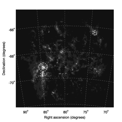
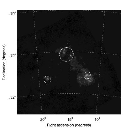
Figure 1: Regions masked in the filtering of SPT time-ordered data. Top panel: 500 $\mu$m map of the LMC from the Herschel HERITAGE survey with the three masked LMC regions indicated by dashed circles (see Table 1 for exact locations). Bottom panel: 500 $\mu$m map of the SMC from the Herschel HERITAGE survey with the three masked SMC regions indicated by dashed circles (see Table 1 for exact locations).

The individual-observation maps in each observing band are combined into full coadded maps using inverse-variance weighting. If the data from one observing band in one individual observation has too few detectors that pass cuts, or if any obvious artifacts are seen when the single-observation map is visually inspected, the map from that observation is not included in the coadded map. Of the 14 individual LMC field observations, 10 are used in the 1.4 mm coadd, 12 in the 2.0 mm coadd, and 12 in the 3.2 mm coadd. Of the four individual SMC field observations, three are used in the 1.4 mm coadd and all four at 2.0 and 3.2 mm. The most common reason for detectors failing cuts is poor weather, which affects the shorter wavelengths more severely (because of the spectral dependence of atmospheric noise at millimeter wavelengths—see, e.g., Bussmann et al. 2005).

In addition to the coadded signal maps, we create coadded null maps for each observing band and field. We combine these maps with Planck HFI null maps in the same way as signal maps are combined, such that the combined null maps can be used in estimating the noise contribution to the uncertainty on any quantity estimated from the combined signal maps. For SPT, we create null maps by subtracting maps made from data in right-going telescope scans only from maps made from data in left-going telescope scans only (divided by two). Any true sky signal should difference away in this operation, leaving an estimate of the instrumental and atmospheric noise. The individual-observation null maps are combined in the same way as the individual-observation signal maps, except that an additional layer of differencing is performed by multiplying one half of the observations by -1. Despite this double differencing (left minus right, multiplying half the individual-observation maps by -1), some small artifacts are visible in the null maps at the location of the brightest regions of the two fields—most notably at the location of 30 Doradus in the LMC. These are due to slight differences in weights and filtering in the left-going and right-going maps, and the amplitude of the artifacts are at most 1% of the amplitude of the original features.

2.1.3 Angular Response Function

As mentioned above, the true instrument beam in each SPT observing band—i.e., the response to a point source as a function of angular offset from the source that would be measured in the absence of any processing to the data—is well-approximated by an azimuthally symmetric Gaussian. These beams are estimated from a combination of dedicated observations of planets and measurements of bright point sources in the SPT-SZ survey field (for details, see Schaffer et al. 2011). The effect of the filtering of SPT data is to modify this angular response function—i.e., to alter the effective instrument beam. Each filtering step has a specific impact on the effective beam. The polynomial subtraction imparts slight negative lobes to the beam in the scan direction—in this case R.A. or $x$—while the module-based filtering imparts an isotropic negative ring at roughly half the scale of a module, or $\sim 10$ arcmin. The anti-aliasing filter smooths the data in the scan direction at or just above the pixel scale (0.25 arcmin); this smoothing is negligible compared to the size of the true beam. All of these effects are represented more cleanly in the two-dimensional Fourier domain, and we use Fourier methods to estimate and represent the response function in this work.

The filter response function is estimated using simulated observations. One hundred independent simulated skies are created, in which the sky signal is white noise convolved with a Gaussian with FWHM equal to 0.75 arcmin. For each simulated sky, a simulated version of the full time-ordered data in each real observation of the LMC or SMC field is created using the telescope pointing and detector focal plane locations. These simulated time-ordered data are then filtered and made into a map in the same manner as is used for the real data, including detector cuts and weighting. The individual-observation maps are combined into full coadded maps using the same procedure and weighting as for the real data. For each of the 100 simulated skies, the square of the two-dimensional Fourier transform of the coadded map is divided by the known input (2d) power spectrum. These 100 estimates are averaged, and the square root of the result is our estimate of the 2d filter response function. We multiply this (in Fourier space) by the instrument beam to create the full beam-plus-filtering response function.

Figure 2 shows the full two-dimensional Fourier-domain angular response function (beam plus filtering) for the 2.0 mm SPT data used in this work. The filter part of the response functions for the 1.4 and 3.2 mm data are nearly identical to the filter part of the 2.0 mm response function. The effect of each filtering step is confined to a specific region of 2d Fourier space. The polynomial subtraction acts as a one-dimensional high-pass filter, suppressing modes at $k_{x}<100$, while the module-based filter acts as an isotropic high-pass, suppressing modes at $k<1000$, where $k$ is angular wavenumber ($k(\lambda)=2\pi/\lambda$ for wavelength $\lambda$ in radians), and $k_{x}$ is the Fourier conjugate of the scan direction. The anti-aliasing filter acts as a scan-direction low-pass filter with a cutoff at $k_{x}\simeq\num{20000}$; however the effect of this low-pass is dominated by the isotropic low-pass of the instrument beam and is not visible in Figure 2.

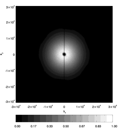
Figure 2: Two-dimensional Fourier-domain angular response function for the 2.0 mm SPT data used in this work. The response function is the product of the instrument beam or point-spread function and the filtering performed on the data. The isotropic suppression of power at $k_{x}\simeq k_{y}\simeq 0$ is from the subtraction of a common mode and two slopes across each detector module at each time sample. The thin line of zero power along $k_{x}=0$ is from the subtraction of a fifth-order polynomial from the data from each detector individually on each scan across the field. The isotropic rolloff at high $k$ is due to the beam.

Finally, we note that the clean representation of the filter response function in 2d Fourier space is to some degree dependent on the projection used to map the curved sky onto a flat, 2d grid. In particular, any filtering that acts on single-detector time-ordered data will result in an effective map-space filter along the scan direction on the sky. Any projection in which the scan direction (R.A.) corresponds to the $x$ axis of the 2d map will localize this filtering in 2d Fourier space to a particular region of 1d angular frequency or wavenumber $k_{x}$. This makes it easy to identify which Fourier modes in the map have been downweighted by the filtering and to replace those modes with modes from the corresponding Planck HFI map. The downside of such a projection is that the mapping of R.A. to $x$ everywhere in the map necessarily leads to angular distortions at the map edges. Such a projection is not optimal for representing the true instrument beam in 2d Fourier space; an angle-preserving projection such as the ZEA projection is more appropriate for dealing with the beam. The maps used to create the representation of the filter function in Figure 2 were made in a simple Cartesian projection, but all other maps in this analysis are made in the ZEA projection.

2.1.4 Noise Estimation

To combine SPT data with Planck HFI data in a nearly optimal way, we need a measure of not only the angular response function for each instrument but also a measure of the noise in each data set. For SPT, the noise is most cleanly represented in the two-dimensional Fourier domain (as was the case with the SPT angular response function). We estimate the 2d noise power spectrum by coadding the single-observation maps with half the maps multiplied by -1, taking the Fourier transform of the result and squaring, and repeating many times with the negative sign assigned to a different set of single-observation maps each time. For the SMC field, there are not enough single-observation maps to get a good noise estimate with this technique, so we use the LMC field estimate scaled by the ratio of observing depth for our SMC field estimate. We note that using a single 2d Fourier estimate for the noise over an entire field assumes that the noise properties are uniform over the field. This is a very good approximation for the SPT maps in this work, except for small regions at the edges of the fields which are not used in the combination with Planck HFI data.

2.1.5 Filter Deconvolution

In preparation for combining the SPT maps with Planck HFI maps, we deconvolve the filter angular response function from the maps, and we modify the noise estimates to account for this deconvolution. We perform this deconvolution in 2d Fourier space: after first multiplying the map by a real-space apodization window, we Fourier transform the map, multiply in Fourier space by the reciprocal of the filter response function, and inverse Fourier transform. To avoid numerical issues, we set the reciprocal of the filter response to zero in any region of 2d Fourier space in which the filter response is less than 0.01. This conditioning step is taken into account when we combine the SPT and Planck maps. We account for the deconvolution in the SPT noise estimates by multiplying the 2d Fourier-space noise estimates by the (conditioned) reciprocal of the filter response.

Note that we only deconvolve the azimuthally symmetric, low-$k$ part of the filter response (the part of Fourier space in which the data can be adequately replaced with Planck data) while leaving the low-$k_{x}$, high-$k_{y}$ part of the response function in the map. This means that in the final, combined maps, a small fraction of angular modes will be missing from the data (except in the regions which were masked during this filtering step). As can be seen from Figures 2 and 5, after combining with Planck data, modes will be missing from a small area at $k_{x}\lesssim 100$ and $k_{y}\gtrsim 2000$. See Section 4.1 for a discussion of the effects of ignoring this small fraction of missing data in the final maps.

2.1.6 Astrometry Check

As discussed in detail in Schaffer et al. (2011), the reconstruction of the pointing (the instantaneous sky location viewed by every detector at every time sample) for the SPT is based on daily measurements of the Galactic HII regions RCW38 and Mat5a, supplemented with information from thermal, linear displacement, and tilt sensors in the telescope. The typical precision in this reconstruction is 7 arcsec (as measured by the rms variation in bright source positions over many individual observations of a field). The overall astrometric solution for SPT maps is refined by comparing to source positions in the Australia Telescope 20 GHz Survey (AT20G) catalog (Murphy et al., 2010), which are tied to very long-baseline interferometry calibrators and are accurate at the 1-arcsec level. When we apply this technique to the LMC and SMC fields, we find small (10-15 arcsec) but statistically significant offsets between the original SPT positions and the AT20G positions. We correct these offsets by simply redefining the map centers. The final map centers (which we use to reproject Planck data onto the SPT grid and which we publish in the final combined map FITS files) are R.A. $79.9906^{\circ}$, decl. $-68.4984^{\circ}$ for the LMC and R.A. $14.9849^{\circ}$, decl. $-72.4994^{\circ}$ for the SMC. Based on the analysis in Schaffer et al. (2011) we expect that, after this correction, the astrometry is good to roughly 2 arcsec rms.

2.2 Planck

The primary science goal of the Planck satellite (Planck Collaboration et al., 2014a), launched in 2009 by the European Space Agency, was to map the CMB over the full sky in nine bands, ranging in wavelength from 350 $\mu$m to 1 cm. In this work, we use publicly available Planck data in the three wavelength bands that closely overlap with the three SPT bands. These are three longest-wavelength or lowest-frequency bands on the Planck High-Frequency Instrument (HFI) and have nominal center wavelengths of 1.4, 2.1, and 3.0 mm (nominal center frequencies of 217, 143, and 100 GHz). The instrument beam or point-spread function in these three bands is close to Gaussian and azimuthally symmetric, with FWHM equal to 5.0, 7.1, and 10.0 arcmin at 1.4, 2.1, and 3.0 mm, respectively.

The Planck HFI time-ordered data are combined into maps using an approximation to the minimum-variance solution (Planck HFI Core Team et al., 2011), in contrast to the technique of filtering and naive bin-and-averaging used to make the SPT maps. This results in maps that are unbiased estimates of the true sky signal at all scales except for the effect of the instrument beam and pixelization, and the DC component of the maps, which is set to zero in the HFI mapmaking procedure (Planck Collaboration et al. 2014b; for more discussion of the zero-point treatment, see Section 3.4). Thus, the angular response functions appropriate for the Planck HFI maps are simply the convolution (or Fourier-space product) of the instrument beams and the known pixel window function. For more details on the Planck HFI instrument and data, see Lamarre et al. (2010), Planck Collaboration et al. (2014c), and Planck Collaboration et al. (2016a).

To create Planck HFI maps of the Magellanic Clouds that match the SPT maps described in the previous section, we first take the publicly available full-mission maps in each of the three bands and resample them from their native pixelization onto the 0.25-arcmin oblique Lambert equal-area azimuthal (ZEA) projection used for the SPT maps. For the R.A./decl. center of the target projection, we use the center of the SPT maps derived from the astrometry cross-check with the AT20G survey (see Section 2.1.6 for details). The HFI maps are stored using the full-sky HEALPix pixelization scheme, with the HEALPix $N_{\mathrm{side}}$ parameter set to 2048, leading to $12\times 2048^{2}$ pixels over the full sky, or a pixel scale of 1.7 arcmin. In the resampling to the 0.25-arcmin flat-sky grid, we oversample each 0.25-arcmin pixel by a factor of four to reduce the effect of resampling artifacts.

The Planck maps in the ZEA projection are then matched to the resolution of the SPT maps by dividing the Planck maps in 2d Fourier space by the ratio of the Planck beam to the SPT beam in the closest observing band. The Planck beams used in this operation are the product of the publicly available measured instrument beams and the HEALPix $N_{\mathrm{side}}=2048$ pixel window function. This Fourier-space operation is equivalent to deconvolving the Planck beam from the map and convolving the result with the corresponding SPT beam. At small enough scales (high enough wavenumber $k$), this ratio becomes small enough to cause numerical issues—and becomes increasingly uncertain as the fractional Planck beam uncertainties grow larger—so we artificially roll off the ratio at low values of the Planck beam ($B(k)<0.005$). This roll-off is taken into account when we combine the SPT and Planck maps (see Section 3.3 for details).

We also create null Planck HFI maps—using the publicly available Planck half-mission maps—to combine with the null SPT maps described in Section 2.1.2. We make the null Planck maps by subtracting one half-mission map from the other half-mission map (divided by two) in each band, then resampling to the ZEA projection, and deconvolving the Planck-SPT beam ratio, as done for the signal maps. As was the case in the SPT null maps, there are small artifacts in the Planck null maps at the location of the brightest regions of the two fields, and, as with the SPT null maps, the artifacts are at the percent level or below.

To combine these Planck HFI maps with the SPT maps described in Section 2.1, we need an estimate of the noise properties of the SPT-beam-matched Planck maps. The noise in Planck HFI maps is uncorrelated between pixels (white) to a very good approximation (Planck HFI Core Team et al., 2011), so the Fourier-domain Planck map noise in a uniform-coverage region is well approximated by a single value at all $k$ values or angular scales. Thus, the Fourier-domain map noise in one of the SPT-beam-matched Planck maps is this value divided by the ratio of the Planck and SPT beams, under the assumption that the Planck noise is uniform over the map.

The Planck coverage in the SMC field is quite uniform, only varying by $\pm 12\%$ across the field (corresponding to $\pm 6\%$ variations in noise). The LMC field is near the south ecliptic pole, and the Planck observing strategy results in regions of very high coverage near the ecliptic poles. Approximately 25% of pixels in the LMC field are in such a region (defined as 50% higher coverage than the mode of the distribution in the rest of the field). Using a single value for the noise across the field will result in a slightly suboptimal combination of SPT and Planck data for the high-weight regions. No bias results from this approximation, and the variation of Planck noise across the field will be properly represented in the combined SPT+Planck null maps. For both fields, we estimate the Planck noise by taking the square root of the mean of the variance values for all pixels in the region covered by SPT. The pixel variance values are provided by the Planck team in the same files as the maps.

3 Combining Data From SPT and PLANCK

There are two main steps in the process of optimally combining the SPT and Planck maps described in previous sections. First, the maps are relatively calibrated (or, more specifically, the SPT map is adjusted to match the Planck maps) and converted from CMB fluctuation temperature to brightness or specific intensity (in units of MJy sr^-1) at a fiducial observing wavelength and for an assumed source spectrum. Then the maps from the two instruments are combined into a single map using inverse-variance weights calculated from the noise estimate for each instrument in each field and band. Each of these steps is described in greater detail below.

3.1 Absolute Calibration

Before the SPT and Planck HFI data can be meaningfully combined into a single map, care must be taken to ensure that the two data sets are consistently calibrated—that is, that a true sky signal would produce the same amplitude of response in both data sets (up to differences in the angular response function of the two instruments). Maps from both instruments are stored in units of CMB fluctuation temperature, i.e., the variation in temperature of a blackbody with mean temperature 2.73K that would produce the detected signal. The absolute calibration of the Planck maps used in this work is taken from the annual modulation of the CMB dipole due to the motion of the satellite around the solar system barycenter (Planck Collaboration et al., 2016a). The fractional statistical uncertainty on this calibration is significantly less than 1%. This calibration can be checked by comparing the CMB power spectrum measured with Planck to the CMB power spectrum measured by the WMAP team, who also calibrate their data off of the modulation of the CMB dipole, using internal WMAP measurements. The CMB power spectrum measurements from the two instruments agree to better than 1% in power (0.5% in CMB fluctuation temperature, Planck Collaboration et al. 2016b).

The SPT absolute calibration is obtained by matching the small-scale (high-multipole) CMB power spectrum measured with SPT and published in George et al. (2015) with the Planck CMB power spectrum over the same multipole range ($670<\ell<1170$, where $\ell$ is multipole number and, over small patches of sky, is equivalent to angular wavenumber $k$ as defined in Section 2.1.3). The fractional statistical uncertainty on this calibration is roughly 2.5% (in temperature) at 1.4 mm and 1.0% (in temperature) at 2.0 and 3.2 mm.

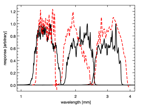
Figure 3: Bandpass functions, or instrument response as a function of wavelength, for SPT-SZ and the lowest three bands of Planck HFI. Planck bands are shown by the solid black lines, while SPT-SZ bands are shown by the dashed red lines. The normalization of the bandpasses is arbitrary.

3.2 Spectral Matching

As discussed in the previous section, the absolute calibration of both the SPT and Planck data used here is based on a source with an emission spectrum described by fluctuations around a 2.73K blackbody, i.e., $I(\lambda)\propto dB/dT(\lambda,2.73K)$, where $B(\lambda,T)$ is the Planck blackbody function. If the SPT and Planck bands were infinitely narrow, or if they had finite width but were identical in response as a function of wavelength (or bandpass), the calibration step described above would be sufficient for matching the SPT and Planck maps of a source with an arbitrary emission spectrum. In reality, the SPT and Planck bands have fractional widths of order 30%, and there are small but significant differences in the bandpass functions for the two instruments, as shown in Figure 3. (The publicly available Planck bands were downloaded from the same server as the maps and instrument beams.)

Because of this small bandpass mismatch, and because the emission from the Magellanic Clouds is not expected to have a $dB/dT(\lambda,2.73K)$ spectrum, we need to apply some further correction factor to match the SPT and Planck responses to the emission from the Magellanic Clouds. The size of that correction depends on the spectral energy distributions (SEDs) at each point within the LMC and SMC and the different SPT and Planck bandpass functions. To choose the appropriate spectral matching factor, we need some prior information on the SEDs of the Magellanic Clouds. Fortunately, the SEDs can be approximated by power laws with a limited range of index. In the following section, we use Planck data in the bands under investigation here and in the neighboring HFI bands to estimate the SEDs of the LMC and SMC at the angular scales accessible to Planck.

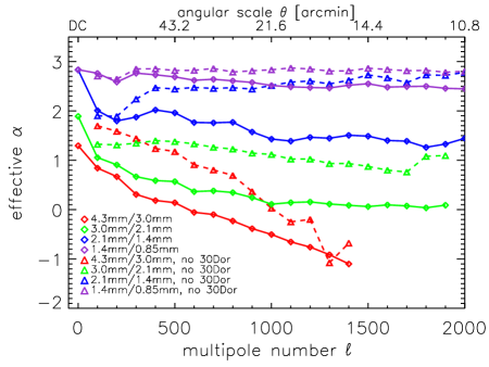
(a) LMC

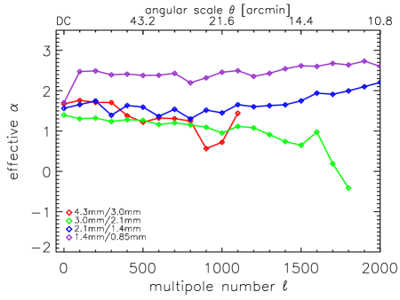
(b) SMC

Figure 4: Effective power-law index $\alpha$ as a function of angular scale or multipole number $\ell$ for four combinations of Planck bands in the LMC (Left Panel) and SMC (Right Panel). The $\ell=0$ value is calculated using the ratio of integrated emission from the full LMC or SMC region, while all other values are calculated using the ratio of the (beam-corrected) power spectra of the Planck maps in each pair of bands. In the left panel, the solid lines show the effective $\alpha$ from the entire LMC region, while the dashed lines show the effective $\alpha$ with 30 Doradus excluded. (In all cases, lines are only drawn for values of $\ell$ at which the beam window function for the longest-wavelength band is above 5% of peak value and for which effective $\alpha$ is well-defined.)

3.2.1 Spectral Energy Distributions of the Magellanic Clouds from Planck-only Data.

In this section, we use Planck data from 0.85 mm to 4.3 mm to estimate the SEDs of the LMC and SMC at Planck angular scales. One complication to this process is evident from Planck-only maps of the Magellanic Clouds in Figure 1 of Planck Collaboration et al. (2011). For example, in the LMC, the dust emission (traced by the 0.35 mm or 857 GHz map) is quite diffuse and covers the entire region, while the synchrotron emission (traced by the 10.5 mm or 28.5 GHz map) is concentrated in bright regions such as 30 Doradus. This makes it unlikely that a single SED will be sufficient to describe the emission across the full extent of the LMC and SMC.

A more quantitative view of this issue is provided in Figure 4, which shows the effective power-law index $\alpha$ (defined assuming specific intensity $I\propto\lambda^{-\alpha}$) in the LMC and SMC as a function of angular scale or multipole number $\ell$ for four combinations of bands: 4.3 mm$/$3.0 mm, 3.0 mm$/$2.1 mm, 2.1 mm$/$1.4 mm, and 1.4 mm$/$0.85 mm. The DC ($\ell=0$) value is calculated using the ratio of integrated emission for each pair of bands given in Table 2 of Planck Collaboration et al. (2011), while all other values are calculated using the ratio of the power spectra of the Planck maps in each pair of bands (corrected by the square of the ratio of beam window functions of the two bands). The solid lines show the effective $\alpha$ from the entire LMC and SMC regions, while the dashed lines in the left panel show the effective $\alpha$ for the LMC with 30 Doradus excluded. (Note that values for a particular pair of bands are only shown for values of $\ell$ at which the beam window function of both bands is greater than 5% of the peak value and for which effective $\alpha$ is well-defined.) It is clear that the shortest wavelengths are dominated by dust emission at all scales and in all regions, while free-free and synchrotron emission contribute significantly to the small-scale emission at longer wavelengths, particularly in the LMC when 30 Doradus is included.

3.2.2 Matched SPT-Planck Maps for Different SEDs

In light of the observed variation in $\alpha$, we choose to make several different combinations of Planck and SPT maps, each appropriate for a different assumed source spectrum. For each such combination, we convert all six maps (three Planck maps, three SPT maps) from units of CMB fluctuation temperature to units of MJy sr^-1 assuming a power-law emission spectrum $I(\lambda)\propto\lambda^{-\alpha}$, evaluated at the nominal central wavelength of the Planck bands. That is, all six maps are scaled such that they represent an estimate of the specific intensity of a $\lambda^{-\alpha}$ source at a wavelength of 1.4, 2.1, or 3.0 mm. The conversion from CMB fluctuation temperature to specific intensity at a given reference wavelength is performed using the formalism described in Section 3.2.3 of Planck Collaboration et al. (2014d) and the bands shown in Figure 3. The null maps and the Fourier-space noise estimates for each instrument are converted using the same factors used for the signal maps.

Guided by the range of effective spectral indices for the LMC seen in Figure 4, we create five different versions of the SPT and Planck maps, each appropriate for combining the two sets of maps if the true sky emission has a particular spectral index. The values of spectral index we assume for the five versions are $\alpha=\{-1.0,0.0,1.0,2.0,3.0\}$. The magnitude of the error incurred by using a map created assuming an incorrect value of $\alpha$ depends on the width of the bands and the fiducial wavelength used for the conversion. The fractional widths of the three Planck bands are similar, and the fiducial wavelengths we use are the nominal Planck band centers. For these reasons, the difference in conversion factors in the Planck bands is small ($<10\%$) for the range of spectral indices used. This is also the case for the SPT 1.4 mm and 3.2 mm bands, which are similar to the corresponding Planck bands in placement and width. However, the SPT 2.0 mm band is significantly offset from the Planck 2.1 mm band, and the factors to convert data in that band from CMB fluctuation temperature to MJy sr^-1 at the nominal Planck band center vary by 30% between $\alpha=-1$ and $\alpha=3.$ This is the strongest motivation for creating multiple sets of combined maps. If a user of the final data products needs a map appropriate for a non-integer spectral index (or an index outside the range we use) and desires conversion accuracy better than 5% (roughly the difference between the SPT 2.0 mm conversion factors assuming $\alpha=\alpha_{0}$ and assuming $\alpha=\alpha_{0}\pm 1$), we suggest interpolating between maps or extrapolating.

3.2.3 Beam-filling vs. Point-like Sources

A further complication to the calculation of conversion factors between CMB temperature and MJy sr^-1 is the question of beam-filling vs. point-like sources. For diffraction-limited optical systems that couple to a single mode of radiation per polarization, the product of telescope area and beam solid angle ($A\Omega$ or étendue) is equal to $\lambda^{2}$. Both SPT and Planck operate in or near this single-moded, diffraction limit for the bands considered here (Padin et al., 2008; Ade et al., 2010). In the limit of constant telescope aperture illumination as a function of wavelength, the $A\Omega$ from a point-like source will be constant, while the $A\Omega$ for a beam-filling source will go as $\lambda^{2}$. The power received by an optical system from a source scales directly with $A\Omega$, so in this limit the conversion factor calculated for a point source with spectral index $\alpha$ will be equivalent to the conversion factor for a beam-filling source with spectral index $\alpha+2$. For the reasons discussed above, this distinction matters significantly only for the SPT 2.0 mm band, where it is up to a 15% difference. All the conversion factors we use here assume beam-filling sources, mainly because that is how the bands and absolute calibration were measured for both instruments (Schaffer et al., 2011; Planck Collaboration et al., 2014d). There are few isolated features at sub-arcminute scales in the Magellanic Clouds (e.g., Meixner et al. 2013, Figure 14), so this is a safe choice for the SPT bands; the assumption is less safe for Planck, but the differences between beam-filling and point-source conversion factors for Planck are much smaller (at the percent level).

3.3 Combining Maps Using Inverse-variance Weighting

Once the SPT and Planck maps are in a common set of units and are consistently calibrated, and we have estimates of the noise for both maps, it is straightforward to combine them in an optimal (minimum-variance) way using inverse-variance weights. The noise estimates are not perfect, and the combined maps are thus not truly optimal. The degree to which the combined maps are sub-optimal depends on the fidelity of the noise estimates and the assumptions underlying these estimates, particularly that of uniform noise across the entire map. As discussed in previous sections, the SPT noise properties are very uniform across the map in both the LMC and SMC fields, while the Planck noise properties are very uniform in the SMC map but not in the LMC map. (A fraction of the pixels in the LMC have Planck noise that is significantly lower than the mean.) The SPT-Planck combination will be slightly sub-optimal for these map regions, but there is no signal bias; furthermore, the combined SPT-Planck null maps properly reflect this variation in noise in the LMC field.

To combine the maps in a given band, we first Fourier transform each map. At each point in 2d Fourier space $\mathbf{k}=[k_{x},k_{y}]$, we define a weight for each map

$$W(\mathbf{k})=N^{-2}(\mathbf{k}),$$ (1)

where $N(\mathbf{k})$ is the Fourier-space noise estimate. Recall that for Planck  we assume white noise in the raw maps, so that the Fourier-space noise in the SPT-beam-matched maps will be proportional to the ratio of the beams:

$$N_{\mathrm{Planck}}(\mathbf{k})\propto B_{\mathrm{SPT}}(\mathbf{k})/B_{\mathrm{Planck}}(\mathbf{k}).$$ (2)

This ratio is a monotonically increasing function of $k$ and reaches a value of 10 at approximately $k=3700$ at 1.4 mm, $k=2500$ at 2.1 mm, and $k=1900$ at 3.0 mm. Hence, the Planck weights will be down by a factor of 100 at these $k$ values compared to $k=0$. Meanwhile, the SPT maps have had the filter response function deconvolved, so the noise in these maps is given by

$$N_{\mathrm{SPT}}(\mathbf{k})=N_{\mathrm{SPT,orig}}(\mathbf{k})/F_{\mathrm{SPT}}(\mathbf{k}),$$ (3)

where $N_{\mathrm{SPT,orig}}(\mathbf{k})$ is the estimate of the noise from the original maps, and $F_{\mathrm{SPT}}(\mathbf{k})$ is the SPT filter response function. From this it is clear that the Planck weights will be proportional to the square of the ratio of the Planck beam to the SPT beam, while the SPT weights will be reasonably flat (depending on the noise properties in the original maps) except for the regions of Fourier space strongly affected by the filtering, which will have much lower weight. We manually zero the Planck weights at any values of $\mathbf{k}$ at which the value of the Planck beam is lower than 0.005, and we manually zero the SPT weights at values of $\mathbf{k}$ at which the azimuthally symmetric part of the SPT filter response is less than 0.01.

The azimuthally averaged values of $N^{2}_{\mathrm{Planck}}(\propto W^{-1}_{\mathrm{Planck}})$ and $N^{2}_{\mathrm{SPT}}(\propto W^{-1}_{\mathrm{SPT}})$ as a function of $k$ in both fields are shown for the 2.1/2.0 mm bands and an assumed spectral index $\alpha=2.0$ in Figure 5. For comparison, we also show $N^{2}_{\mathrm{SPT}}$ at 2.0 mm from a typical field in the 2500-square-degree SPT-SZ survey (in which the typical field was observed a factor of roughly 10 longer than the total LMC observations used in this work). Plots of $N^{2}_{\mathrm{Planck}}$ and $N^{2}_{\mathrm{SPT}}$ in the 1.4 mm and 3.0 mm bands look similar, except that the Planck/SPT crossover point is at higher $k$/$\ell$ for the 1.4 mm band.

Figure 5: Noise power as a function of angular wavenumber $k$ or multipole number $\ell$ for the Planck 2.1 mm band and the SPT 2.0 mm band. The solid lines show the noise power in the LMC field; dashed lines show the noise power in the SMC field. The SPT noise is measured after deconvolving the filter response function, while the Planck noise is measured after matching to the SPT beam (see Section 3.3 for details). In all cases, the assumed spectral index for the emission is $\alpha=2.0$. The small bump in the SPT noise at $k=3600$ is due to a noise feature associated with the 6-arcmin elevation step between scans (see Section 2.1.1 for details). The thin dot-dashed line shows the 2.0 mm noise power for a typical field in the SPT-SZ survey (calculated in the same manner as for the LMC and the SMC curves in this plot).

The combined map in Fourier space is then simply

$$M_{\mathrm{comb}}(\mathbf{k})=\frac{W_{\mathrm{SPT}}(\mathbf{k})M_{\mathrm{SPT}}(\mathbf{k})+W_{\mathrm{Planck}}(\mathbf{k})M_{\mathrm{Planck}}(\mathbf{k})}{W_{\mathrm{SPT}}(\mathbf{k})+W_{\mathrm{Planck}}(\mathbf{k})},$$ (4)

where $M(\mathbf{k})$ indicates a Fourier-space map. We note that there are no modes for which both the Planck and the SPT weights have been manually zeroed; for all modes of interest, Equation 4 is well defined. We then inverse Fourier transform to obtain the combined map in real space $M_{\mathrm{comb}}(x,y)$.

Finally, to limit the effect of noise near the beam scale, we make three smoothed versions of each combined map at 1.4 and 2.1 mm and two smoothed versions of each map at 3.0 mm. For the 1.4 and 2.1 mm maps, we make a version that is only slightly smoothed compared to the SPT beam: we convolve these maps with the difference between the SPT beam at that wavelength and a 1.5-arcmin FWHM Gaussian. (We do not make this version of the 3.0 mm map, because the SPT beam itself is roughly a 1.7 arcmin FWHM Gaussian.) For maps in all wavelength bands, we make versions with 2.0 and 2.5-arcmin resolution by convolving the combined SPT-resolution map with the difference between the SPT beam and a 2.0 or 2.5-arcmin FWHM Gaussian. We provide maps at different resolutions in an attempt to balance the requirements of low noise and high angular resolution. End users of these maps that are interested in the smallest-scale features of the Magellanic Clouds should use the highest-resolution maps and pay the penalty of slightly higher noise, while users interested in, for example, performing few-arcminute scale photometry on the maps should use the lower-resolution versions with reduced noise. Users can also of course perform their own filtering on the data—for example, loading one of the 1.5-arcmin-resolution maps into the SAOImage ds9 software and applying the Gaussian smoothing kernel with a kernel radius of seven pixels very closely reproduces the 2.5-arcmin-resolution version of that map.

3.4 Treatment of Galactic Foregrounds and Map Zero Level

A primary use of the combined SPT-Planck maps described in this work is expected to be aperture photometry on localized regions of the LMC and SMC. In this application, any emission from sources other than the Magellanic Clouds will either act as a source of bias or extra variance, depending on the whether that emission varies significantly over the LMC or SMC field. In particular, the mean value of any source of non-Magellanic-Clouds emission will act as a bias, so we attempt to remove the mean of all such sources from the combined SPT-Planck maps.

In our combining procedure, the DC ($k=0$) weight for the SPT maps is always set to zero, so the mean across the combined maps will be equal to the mean of the Planck map. As discussed in Section 2.2, the Planck maps are constructed so that the mean across the full sky is identically zero. However, the expected mean of the Galactic signal and the cosmic infrared background (CIB) are manually added back to the Planck maps before public release—though the mean emission from the 2.73K CMB is not (Planck Collaboration et al., 2014b). Though the CIB monopole is much smaller than the mean Galactic signal, we subtract it from the maps nonetheless. The variance of the residual CIB fluctuations is completely negligible compared to noise and CMB fluctuations, and we ignore it.

The signal from our own galaxy is not a random field like the CMB or CIB, so we do not subtract the full-sky mean from our maps but rather an estimate of the mean in the direction of the LMC or SMC. We estimate this mean in each Planck band by taking the mean signal quoted at 0.35 mm (857 GHz) in Planck Collaboration et al. (2011) toward each region and scaling by the Galactic cirrus spectral energy distribution quoted in Planck Collaboration et al. (2015). This assumes the Galactic foreground signal is dust-dominated across all the frequencies treated here, an assumption supported by Figure 4 of Planck Collaboration et al. (2011). The residual variance across the LMC and SMC is estimated in Planck Collaboration et al. (2011) to be $\ll 10^{-3}\ \mathrm{MJy}\ \mathrm{sr}^{-1}$ rms in all bands and in both regions, a factor of at least 10 below the CMB fluctuation level (see Section 4.3.2), and we ignore this source of variance as well. The variance from CMB fluctuations is discussed in detail in Section 4.3.2.

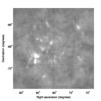
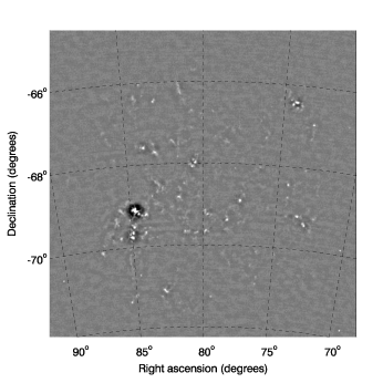
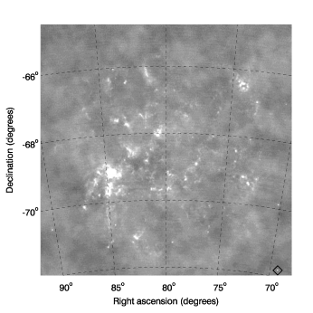
(a) Planck-only, SPT-only, and Planck+SPT maps of the 7-by-7-degree LMC field

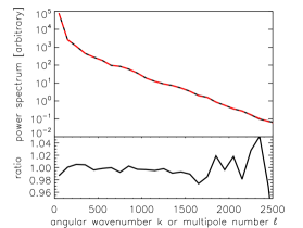
(b) Planck+SPT map matched to the original Planck resolution (Left Panel); power spectrum of the Planck-only map and the Planck-matched combined map and their ratio (Right panel)

Figure 6: An illustration of the process of combining SPT and Planck data on the LMC field, and a demonstration that the combined map is dominated at large scales by the Planck information, as expected. Top row: The Planck 2.1 mm map, projected from the original HEALPix format onto the 7.5-by-7.5-degree ZEA grid (Left Panel); the SPT 2.1 mm map on the native 7.5-by-7.5-degree ZEA grid (Center Panel); and the combined 2.1 mm map at 1.5 arcmin resolution (Right Panel). Bottom row: The combined 2.1 mm map convolved with a kernel equivalent to the ratio of the 2.1 mm Planck beam to a 1.5-arcmin Gaussian to match the resolution of the original Planck map (Left Panel); and the power spectrum of the maps in the upper left (black solid line) and lower left (red dashed line) panels, as well as their ratio (Right Panel, see Section 4.1 for details on the power spectrum calculation). The visual agreement between the maps in the upper left and lower left panels demonstrates that the combined map reverts to the original Planck map when the higher-resolution SPT information is smoothed away. This is shown quantitatively in the power spectrum ratio, which is within 5% of unity at all scales at which there is significant information in the Planck-resolution maps. The negative shadowing around regions of strong emission in the SPT-only map is due to the common-mode subtraction (see Section 2.1.3) and goes away when the information in these angular modes is added from the Planck map. For these images and this calculation, we have used the combined map constructed assuming an emission spectrum $I(\lambda)\propto\lambda^{-2}$. The black diamond in the upper-right panel indicates the position of PKS 0437-719, the extragalactic source used for the resolution test shown in Figure 7.

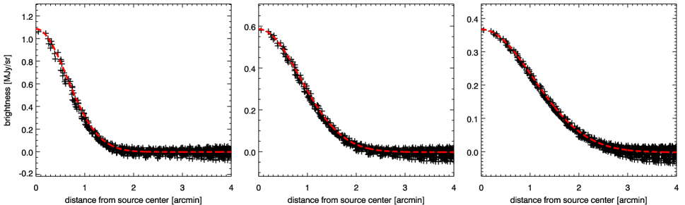
Figure 7: Pixel values vs. angular distance from the radio source PKS 0437-719, the brightest background source in the LMC field. (The location of PKS 0437-719 is indicated by a black diamond in the upper-right panel of Figure 6.) This source is expected to be point-like at SPT resolution. Pixel values are extracted from the 2.1 mm combined SPT-Planck maps that are expected to have angular response functions equal to 2d Gaussians with FWHM of 1.5 (left panel), 2.0 (center panel), and 2.5 (right panel) arcmin. In each panel, the extracted pixel values are shown as black crosses, and the expected angular response function (with amplitude taken from a fit of the map cutout to a 2d Gaussian) is shown as a dashed red line. The measured shape of this radio source in the maps is consistent with the expected angular response function.

4 Results

The primary result of this work consists of two sets of 40 maps (one set each for the LMC and SMC fields). These maps are 1800-by-1800 pixels and 1200-by-1200 pixels—or 7.5-by-7.5 degrees and 5-by-5 degrees—for the LMC and SMC fields, respectively. Each set of 40 maps consists of eight maps each created assuming one of five emission underlying spectra (power-law emission $I(\lambda)\propto\lambda^{-\alpha}$ with spectral index $\alpha=\{-1.0,0.0,1.0,2.0,3.0\}$). For each value of spectral index, the eight maps consist of three maps of combined SPT and Planck data at 1.4 mm (one each at resolutions of 1.5, 2.0, and 2.5 arcmin), three maps of combined SPT and Planck data at 2.1 mm (one each at resolutions of 1.5, 2.0, and 2.5 arcmin), and two maps of combined SPT and Planck data at 3.0 mm (one each at resolutions of 2.0, and 2.5 arcmin).

In this Section, we perform some simple tests to verify certain assumptions or expectations about the maps, in particular their resolution and their fidelity to the original Planck data. These tests and the results are discussed in Section 4.1. In Section 4.2, we show images from a selection of maps, centered on certain features of interest in the LMC and SMC, and discuss the properties of the maps evident from these images. Finally, we discuss the instrumental and astrophysical noise properties of the maps in Section 4.3.

4.1 Combined Map Checks

In this section, we perform three checks on the combined SPT+Planck maps and the process used to construct them. First, we use simulated observations to calculate the effect of ignoring the thin stripe of low-$k_{x}$, high-$k_{y}$ modes removed by the SPT scan-direction filtering and not replaced with Planck data (see Section 2.1.5 for details). Next we verify the fidelity of the final, combined maps by comparing them with the original Planck data. Because of the nature of the SPT and Planck data, in particular the filtering of large angular scales (low-$k$ Fourier modes) from the SPT data (see Section 3.3 for details), we expect the combined maps to be dominated on large scales (small values of wavenumber $k$) by the information from the Planck maps, and we check that this expectation is borne out. Finally, we confirm the expected angular response function of the final, combined, Gaussian-smoothed maps: If our measurements of the Planck and SPT beams and of the SPT filter response are accurate, then we expect that the only angular response function in the final maps is the Gaussian smoothing (except for adjustments of the overall mean intensity in the LMC or SMC region—see Section 3.4 for details).

To estimate the bias that results from ignoring the small fraction of Fourier modes removed from the SPT maps and not replaced by Planck data, we create simulated maps with the same filtering as the real SPT maps and combine them with simulated Planck maps of the same mock skies. We then perform aperture photometry on the simulated combined SPT+Planck maps and compare the results to aperture photometry on the true, underlying mock skies. We create many mock skies with features on different angular scales, and we perform aperture photometry using many different aperture radii. For features on scales of 1 to 10 arcminutes and aperture radii in the same range, we find a typical bias of $<2\%$ and a maximum bias of $<4\%$ resulting from the missing low-$k_{x}$, high-$k_{y}$ modes.

We verify the fidelity to the original Planck maps in two ways. First, in Figure 6 we show four versions of the 2.1 mm, $\alpha=2.0$ map of the LMC field: 1) the Planck data (not beam-matched to SPT) directly projected onto the final ZEA grid; 2) the filtered SPT data projected onto the final ZEA grid; 3) the 1.5-arcmin-FWHM version of the final map; 4) the map in (3) convolved with the difference between a 1.5-arcmin-FWHM Gaussian and the Planck 2.1 mm beam. There is strong visual agreement between the original Planck map and the final maps smoothed to Planck resolution. To make this more quantitative, we calculate the power spectrum of each of these maps and plot these and the ratio between them in Figure 6. To avoid noise bias in the power spectrum, we create two versions of each map using only half the SPT or Planck data and calculate a cross-spectrum between the two half-depth maps. We mask the region around 30 Doradus before computing the power spectrum, as it otherwise dominates the power on all scales. As shown in Figure 6, the power spectrum calcluated from these two maps agrees to better than 5% at all scales on which there is significant power in the maps. These two results support the idea that these maps are dominated by Planck information on scales larger than the Planck beam.

Second, we perform aperture photometry on the LMC field and SMC field maps, centered at R.A.=$78.88^{\circ}$, declination=$-68.50^{\circ}$ and R.A.=$16.07^{\circ}$, declination=$-72.86^{\circ}$, respectively, and in apertures of radius $0.5^{\circ}$, $1^{\circ}$, and $2^{\circ}$. We then perform aperture photometry on the Planck maps in their original HEALPix format, and we compare the resulting flux values. The fluxes from aperture photometry on the maps presented here agree with the results of aperture photometry on the original Planck maps to no worse than 2% in all combinations of wavelength band, field, and aperture size. These results are consistent with the aperture photometry on simulated maps.

Finally, we expect these maps to be nearly unbiased estimates of the sky brightness at all angular scales; the only response function expected is the 1.5, 2.0, or 2.5-arcmin FWHM Gaussian smoothing kernel and the small strip of modes missing at low $k_{x}$ and high $k_{y}$. We confirm this expectation by taking a cutout of the 2.1 mm ($\alpha=2.0$) map of each resolution around the brightest background point source in the LMC field, the radio source PKS 0437-719 (which is expected to be point-like at SPT resolution, Healey et al. 2007). The location of this source is indicated by a black diamond in the upper-right panel of Figure 6. The brightness of the map at each resolution as a function of distance to this source is plotted in Figure 7. Overplotted in each case is the expected response to a point source in that map, namely a 1.5, 2.0, or 2.5-arcmin FWHM Gaussian. The measured response is consistent by eye with the expected response. If we fit the map cutouts to a model of a two-dimensional Gaussian, the geometric mean of the best-fit FWHM along the two axes are 1.45, 1.98, and 2.51 arcmin at the three resolutions (within $\sim$3% of the expected FWHM of 1.5, 2.0 and 2.5 arcmin).

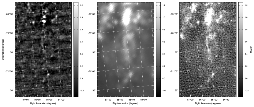
(a) LMC, molecular ridge below 30 Doradus, 1.4 mm, 1.5-arcmin resolution

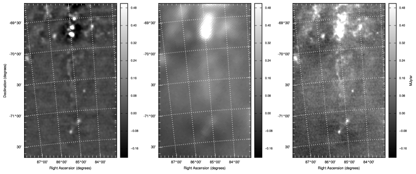
(b) LMC, molecular ridge below 30 Doradus, 2.1 mm, 1.5-arcmin resolution

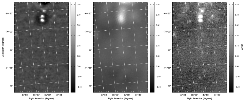
(c) LMC, molecular ridge below 30 Doradus, 3.0 mm, 1.8-arcmin resolution

Figure 8: Combined SPT-Planck maps of the molecular ridge below 30 Doradus in the LMC. This subfield of the LMC is chosen to emphasize the gain in resolution between Planck alone and Planck+SPT. The field in shown in SPT data alone (Left), in Planck data alone (Center), and combined (Right) in all three wavelength bands. The units of the maps are MJy sr^-1, and the SPT and Planck data that make up the maps have been converted from CMB fluctuation temperature to specific intensity assuming an underlying emission spectrum $I(\lambda)\propto\lambda^{-2}$.

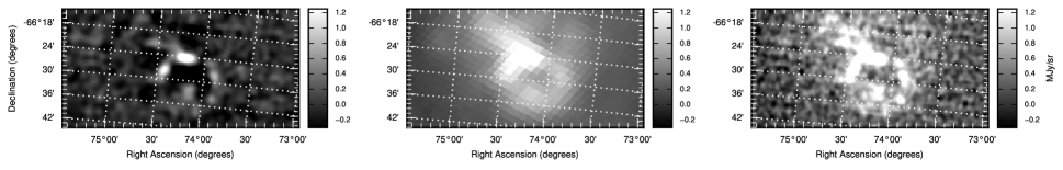
(a) LMC, N11, 1.4 mm, 1.5-arcmin resolution

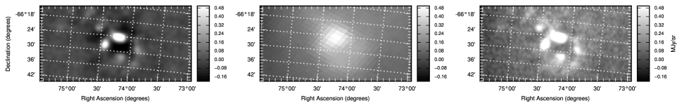
(b) LMC, N11, 2.1 mm, 1.5-arcmin resolution

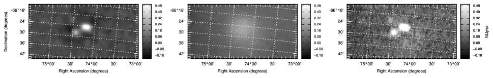
(c) LMC, N11, 3.0 mm, 1.8-arcmin resolution

Figure 9: Combined SPT-Planck maps of the star-forming region N11 in the LMC. This subfield of the LMC is chosen to emphasize the gain in resolution between Planck alone and Planck+SPT. The field in shown in SPT data alone (Left), in Planck data alone (Center), and combined (Right) in all three wavelength bands. The units of the maps are MJy sr^-1, and the SPT and Planck data that make up the maps have been converted from CMB fluctuation temperature to specific intensity assuming an underlying emission spectrum $I(\lambda)\propto\lambda^{-2}$.

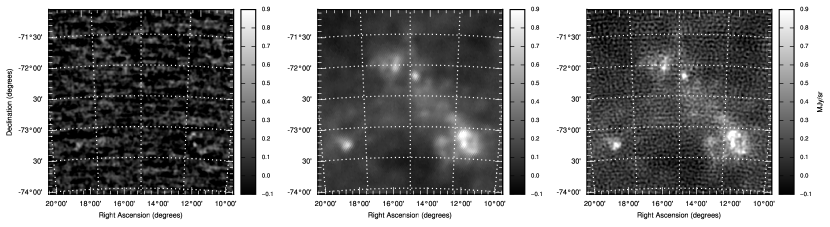
(a) SMC, 1.4 mm, 2.5-arcmin resolution

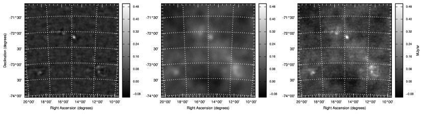
(b) SMC, 2.1 mm, 2.5-arcmin resolution

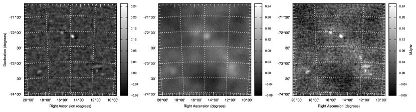
(c) SMC, 3.1 mm, 2.5-arcmin resolution

Figure 10: Combined SPT-Planck maps of the SMC. The field in shown in SPT data alone (Left), in Planck data alone (Center), and combined (Right) in all three wavelength bands. The units of the maps are MJy sr^-1, and the SPT and Planck data that make up the maps have been converted from CMB fluctuation temperature to specific intensity assuming an underlying emission spectrum $I(\lambda)\propto\lambda^{-2}$.

4.2 Selected Map Images

In Figures 8–10, we show cutouts of a selection of Planck+SPT maps centered on features of interest in the LMC and SMC fields. Figure 8 shows the molecular ridge south of 30 Doradus in the LMC (e.g., Ott et al. 2008), Figure 9 shows the star-forming region N11 in the LMC, and Figure 10 shows a 2.5-by-2.5 degree cutout of the full 5-by-5 degree SMC field. In all cases, the maps shown use data converted from CMB fluctuation temperature to specific intensity assuming an underlying emission spectrum $I(\lambda)\propto\lambda^{-2}$. The images of LMC regions (Figures 8 and 9) use maps at 1.5-arcmin resolution for 1.4 and 2.1 mm and maps at 1.8-arcmin resolution for 3.0 mm. The image of the SMC (Figure 10) uses 2.5-arcmin resolution maps at all wavelengths.

In all of the combined maps, it is clear there is ample arcminute-scale structure in the millimeter-wave emission from Magellanic Clouds (particularly the LMC) and that this structure is qualitatively similar in the three wavelength bands used in this work. Comparing the Planck-only map in each figure to the combined map demonstrates the value of adding the higher-resolution SPT data in elucidating this small-scale structure. The one possible exception to this is the 1.4 mm map of the SMC, in which the noise in the SPT map is high enough that the SPT data contributes comparatively little to the combined map. No obvious artifacts are visible in any of these images.

4.3 Noise Properties of the Combined Maps

In this section, we discuss the noise properties of the combined SPT-Planck maps. For the purposes of measuring emission from the Magellanic Clouds, we consider astronomical signal from other sources to be noise. The only significant astronomical contribution to the noise budget in this work is anisotropy in the CMB. We first discuss the contribution to the map noise from the two instruments, then we discuss the contribution from the CMB.

4.3.1 Instrument Noise

Figure 11 shows a real-space representation of the instrument noise contribution to the LMC field map noise, as measured in the combined SPT-Planck null maps. The construction of the null maps for each instrument is described in detail in Sections 2.1.2 and 2.2. We construct combined null maps by combining null maps from each instrument in the same way as the signal maps. Instrument noise is also discernible without differencing away signal in some of the maps shown in Figures 8–10, particularly at 1.4 and 3.0 mm.

In the LMC null maps and in the cutout maps at 3.0 mm, the instrument noise is most visible at the smoothing scale of the maps, as would be expected for noise that was white before smoothing. However, it is possible to discern an isotropic pattern of noise at a different scale in the 1.4 mm maps, particularly in the SMC. This pattern is from pixel-scale Planck noise convolved with the ratio of the SPT and Planck 1.4 mm beams. This ratio is cut off at $k\sim 4000$, which imparts the particular angular scale to the noise pattern. The reason this pattern is more visible in 1.4 mm than at the other wavelengths is the relative depths of the SPT and Planck maps: the ratio of SPT map noise to Planck map noise is significantly higher at 1.4 mm than in the other bands, thus the Planck map contributes to the combination out to $k$ values at which the value of the Planck beam is quite small.

For practical purposes, the most important property of the map noise is the noise rms in map patches of various size—i.e., the expected noise contribution to the uncertainty in the measurement of the brightness of a feature in the maps of a given angular size. In Figure 12, we plot the instrument noise contribution to the measurement of the flux of a feature as a function of the size of that feature. Specifically, this is the standard deviation of 400 measurements of the flux within a circular region of a given diameter in the null map, each measurement with a different (random) center. We also show the contribution of the CMB to this uncertainty (discussed in the next section), and we show both contributions in the case that the flux in an equal-area region around the circular region is subtracted (we refer to this as the compensated top hat flux). In Table 2, we list values of these contributions (for the compensated and uncompensated top hat fluxes) for several values of the region diameter.

(a) LMC null map, 1.4 mm

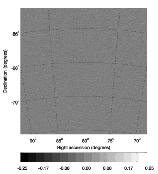
(b) LMC null map, 2.1 mm

(c) LMC null map, 3.0 mm

Figure 11: Combined SPT-Planck null maps of the 7.5-by-7.5-degree LMC field in three wavelength bands. Null maps are created by subtracting one half of the data from the other half and dividing by two. The 1.4 mm and 2.1 mm are at 1.5-arcmin resolution; the 3.0 mm map is at 2.0-arcmin resolution. The units of the maps are MJy sr^-1. The localized feature at roughly [$85^{\circ}$,$-69^{\circ}$] in the 3.0 mm map is a residual of the bright LMC source 30 Doradus (see Sections 2.1.2 and 2.2 for details). For all images, we have used the combined null maps constructed assuming an emission spectrum $I(\lambda)\propto\lambda^{-2}$.

4.3.2 Astrophysical Noise

Comparing Figures 6 and 11, it is clear that there is a diffuse, large-scale contribution to the signal maps in the LMC field that is not in the null maps and hence not part of the instrument noise budget discussed in the previous section. The morphology of this signal is consistent with that of a random Gaussian field with the power spectrum of the CMB and inconsistent with the filamentary structure of high-latitude Galactic emission, indicating that it is likely CMB anisotropy. The signal is present in all three wavelength bands and in both the LMC and SMC maps, and its spectral shape in the three bands is consistent with that of CMB anisotropy and inconsistent with that of thermal dust or synchrotron emission. This signal is not present in shorter-wavelength Herschel-SPIRE maps (see, e.g., Meixner et al. 2013 or Figure 13), indicating it is not Galactic dust emission. The rms temperature fluctuation in the CMB, when measured in patches significantly smaller than a degree, is approximately $100\ \mu\mathrm{K}$, corresponding to roughly 0.04, 0.035, and 0.02 MJy sr^-1 in the three wavelength bands used in this work. This is consistent with the amplitude of the diffuse background in both the LMC and SMC maps.

Anisotropy in the CMB has a much different behavior as a function of angular scale than the instrument noise in these maps: the CMB power is highest on degree angular scales, while the instrument noise is more scale-independent. This leads to different relative contributions of the two noise sources at different scales, as shown in Figure 12 and Table 2. The CMB contribution in this figure and plot are calculated by creating many simulated CMB skies, converting from CMB temperature fluctuation to specific intensity or brightness in each wavelength band, and performing aperture photometry on the simulated maps. As with the instrument noise contribution, the standard deviation of the flux measured in many apertures of a given size around random centers is reported as the expected noise contribution.

The different angular scale dependence of the CMB contribution to the noise means that, on scales of less than about a degree, the noise contribution from the CMB can be suppressed by a simple spatial filtering operation such as subtracting an equal-area region around an aperture in which one wishes to measure a flux. Of course, if there is significant flux in the compensating aperture from Magellanic Cloud features, this operation will not simply difference away the CMB but also bias the aperture measurement. We report expected CMB noise levels (Table 2) for making flux measurements performed with such a compensated top-hat filter, but we caution that such a filter is most appropriate for isolated structures, rather than for crowded fields.

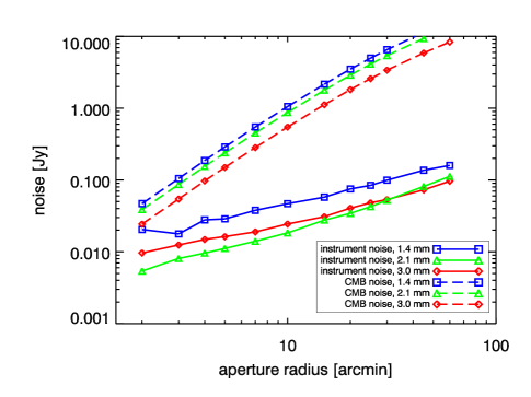
(a) Uncompensated aperture

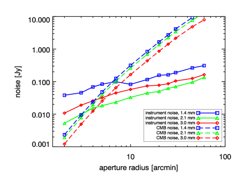
(b) Compensated aperture

Figure 12: Expected contributions from instrument noise and CMB anisotropy to the uncertainty on a measurement of flux in the LMC field within an aperture as a function of aperture size. The instrument noise values in both panels are estimated from the SPT+Planck null maps at 2.0-arcmin resolution, and the CMB values are estimated from simulated CMB maps with 2.0-arcmin resolution. The behavior at 1.5 and 2.5-arcmin resolution is qualitatively similar except at the smallest aperture, and the behavior in the SMC field is nearly identical, but with slightly higher instrument noise values. Values at particular aperture sizes for all map resolutions and both fields are shown in Table 2. Values shown in the left panel are calculated with no compensating negative region around the aperture; values shown in the right panel are calculated with the flux from an equal-area region surrounding the aperture subtracted. For apertures smaller than $\sim 30$ arcmin, this compensation significantly reduces the contribution from the CMB at the expense of increasing the instrument noise contribution (by roughly a factor of $\sqrt{2}$).

5 Comparison with Herschel-SPIRE Maps of the LMC

As mentioned in Section 1, Meixner et al. (2013) have produced maps from the Herschel HERITAGE survey of the Magellanic Clouds. Of all publicly available data on the Magellanic Clouds, these maps are closest in wavelength and resolution to the maps produced here, and comparing the two sets of maps provides both a visual check on the maps produced in this work and insight into the emission processes at work in the Magellanic Clouds. We focus on the LMC here, because the signal-to-noise in the SPT-Planck maps is higher than in the SMC. We further focus on the HERITAGE maps from the Spectral and Photometric Imaging Receiver (SPIRE) instrument rather than from the Photodetector Array Camera and Spectrometer (PACS) instrument, because the SPIRE bands are closer in wavelength to the SPT-Planck bands used here.

In Figure 13, we show images of the LMC and SMC in two representative bands—the SPIRE 500 $\mu$m band and the SPT-Planck 2.1 mm band—at a common resolution. To produce the SPIRE maps, we download the publicly available HERITAGE maps from the NASA/IPAC Infrared Science Archive, reproject them from the native projection and map center to the projection and map center used in this work, and convolve them with a Gaussian kernel with FWHM equal to the quadrature difference between 2 arcmin and the SPIRE beam FWHM in each band.

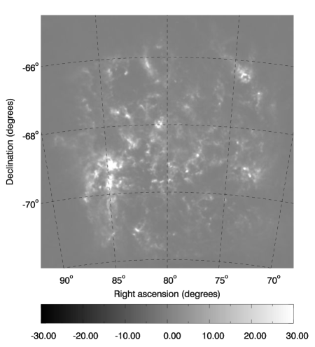
(a) LMC, 500 $\mu$m, 2.0-arcmin resolution

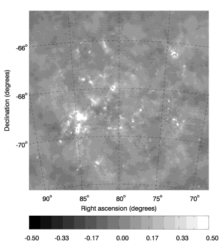
(b) LMC, 2.1 mm, 2.0-arcmin resolution

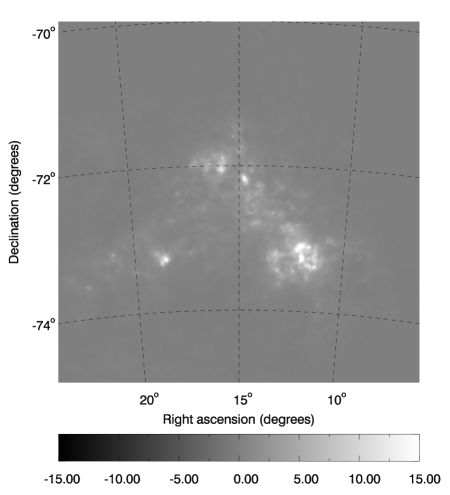
(c) SMC, 500 $\mu$m, 2.0-arcmin resolution

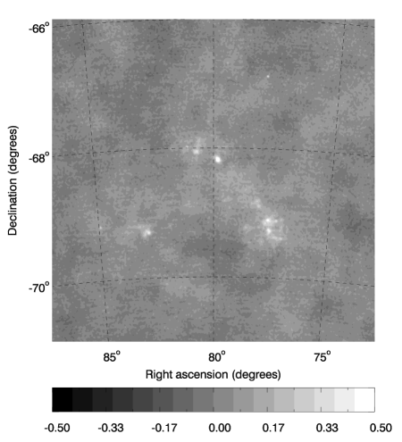
(d) SMC, 2.1 mm, 2.0-arcmin resolution

Figure 13: Herschel-SPIRE and combined SPT-Planck maps of the LMC and SMC. Top row: 500 $\mu$m Herschel-SPIRE map (Left Panel) and 2.1 mm combined SPT-Planck map (Right Panel) of the 7.5-by-7.5-degree LMC field at 2.0 arcmin resolution. Bottom row: 500 $\mu$m Herschel-SPIRE map (Left Panel) and 2.1 mm combined SPT-Planck map (Right Panel) of the 5-by-5-degree SMC field at 2.0 arcmin resolution. The Herschel-SPIRE maps are the publicly available maps from Meixner et al. (2013) and have been reprojected from their original projection and map center to the same projection and map center used for the combined SPT-Planck maps and smoothed with a Gaussian kernel with FWHM equal to the quadrature difference of 2.0 arcmin and the SPIRE beam at each wavelength. The combined SPT-Planck maps were constructed assuming an emission spectrum $I(\lambda)\propto\lambda^{-2}$. The units of all maps are MJy sr^-1.

A high level of common structure is evident between the two bands shown in Figure 13, but the densest, brightest knots of emission are more prominent relative to the diffuse structure in the 2.1 mm map. This is consistent with the indications from Planck-only data in Planck Collaboration et al. (2011) and Section 3.2.1 that the brightest regions have a higher contribution from synchrotron and free-free emission than the filaments, particularly in the LMC. The three-color images in Figures 14 and 15 reinforce this picture. These images combine resolution-matched SPT-Planck 3.0 mm (red) and 2.1 mm (green) and SPIRE 500 $\mu$m (blue) maps (at 2.0 arcmin resolution for the LMC and 2.5 arcmin resolution for the SMC) with a relative scaling such that emission that scales as $\lambda^{-2}$ would appear roughly white. As expected, the filamentary structure of the LMC and SMC appears mostly blue, consistent with thermal dust emission going as $\lambda^{-\alpha}$ with $\alpha>2$, while the dense, bright knots of emission are redder (where they do not saturate the color scale). The diffuse, yellowish background in these images is the CMB, while the red, unresolved sources are background radio galaxies, all of which have counterparts in the 36 cm (843 MHz) Sydney University Molongolo Sky Survey (SUMSS, Mauch et al. 2003).

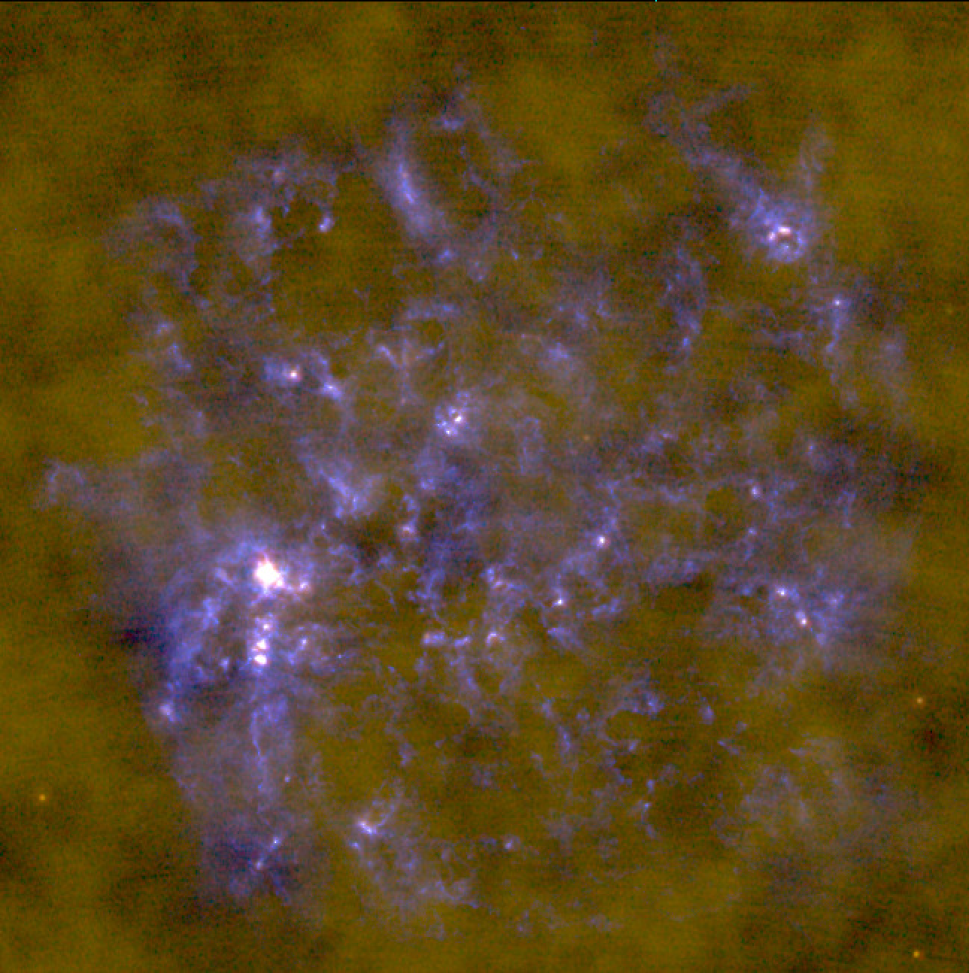
Figure 14: Three-color image of the LMC. Red = SPT-Planck 3.0 mm; Green = SPT-Planck 2.1 mm; Blue = 500 $\mu$m Herschel-SPIRE. The respective scales are $[-0.08,1.0]$, $[-0.08,2.5]$, and $[-0.08,35.0]$ MJy sr^-1, such that a source with a $\lambda^{-2}$ spectrum would appear roughly white. Before combining, all three maps have been convolved with a smoothing kernel such that the resolution in the map is 2.0 arcmin. The diffuse, large-scale, yellowish signal is anisotropy in the CMB. Most of the filamentary structure in the LMC is blue, indicating thermal dust as the primary emission mechanism. The bright knots are in general redder, indicating a higher fraction of free-free or synchrotron emission, consistent with Planck-only results in Planck Collaboration et al. (2011) and Section 3.2.1. (Note that the very brightest regions such as 30-Doradus appear white because they saturate the color scale, not because they are exactly consistent with $\lambda^{-2}$.) The red, point-like sources at the perimeter of the image are background radio sources, all of which have counterparts in the SUMSS catalog (Mauch et al., 2003). This image was produced using STIFF (Bertin, 2012).

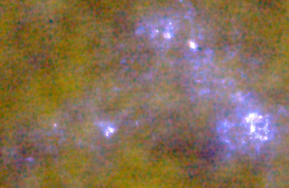
Figure 15: Three-color image of the SMC. Red = SPT-Planck 3.0 mm; Green = SPT-Planck 2.1 mm; Blue = 500 $\mu$m Herschel-SPIRE. The respective scales are $[-0.1,0.4]$, $[-0.1,0.8]$, and $[-0.1,7.0]$ MJy sr^-1, such that a source with a $\lambda^{-2}$ spectrum would appear roughly white. Before combining, all three maps have been convolved with a smoothing kernel such that the resolution in the map is 2.5 arcmin. The diffuse, large-scale, yellowish signal is anisotropy in the CMB. This image was produced using STIFF (Bertin, 2012).

6 Conclusions

We have created maps of the Large and Small Magellanic Clouds from combined SPT and Planck data in three wavelength bands, centered at roughly 1.4, 2.1, and 3.0 mm. These maps—one set of 40 maps each for the LMC and SMC fields—consist of eight maps each created assuming different underlying emission spectra (power-law emission $I(\lambda)\propto\lambda^{-\alpha}$ with different spectral indices). We have created maps at three different final resolutions (Gaussian FWHM of 1.5, 2.0, and 2.5 arcmin) in the 1.4 and 2.1 mm bands and two different resolutions (2.0 and 2.5 arcmin) in the 3.0 mm band. For each set of maps assuming a given spectral index, we have calibrated and color-corrected the SPT data to match the Planck data in a given band. We have then used knowledge of the noise properties and angular response function for each map to make an inverse-variance-weighted combination of the two instruments’ data as a function of angular scale.

We have performed several consistency checks on the resulting maps, and we have estimated the noise contributions from instrumental and astrophysical components to flux measurements performed on those maps. We have visually compared the maps of the LMC to FIR/submm maps from the Herschel HERITAGE survey and found clear common structure and evidence of a dependence of emission mechanism on brightness and/or density.

These maps extend the angular resolution of mm-wave studies of the Magellanic Clouds down to $\sim$1 arcmin—or, equivalently, extend the wavelength coverage of arcminute-scale maps of the Magellanic Clouds into the mm-wave regime. We expect these maps to be useful resources in studies of star formation in diverse environments and to increase our understanding of the physical processes at work in our two nearest neighbor galaxies. All data products described in this paper are available for download at http://pole.uchicago.edu/public/data/maps/magclouds and from the NASA Legacy Archive for Microwave Background Data Analysis server.

Table 2: Noise contributions as a function of aperture diameter for the maps constructed assuming spectral index $\alpha=2.0$ and with 2.0 arcmin resolution.

Field	Aperture Radius	Compensated?	Instrument Noise			CMB Noise
	[arcmin]		[mJy]			[mJy]
			1.4 mm	2.1 mm	3.2 mm	1.4 mm	2.1 mm	3.2 mm
LMC	2	N	20.5	5.4	9.6	46.9	38.7	24.3
	3	N	17.8	8.1	12.5	104.9	86.7	54.4
	4	N	27.9	9.6	14.9	187.3	154.8	97.2
	5	N	28.8	11.1	16.3	289.1	238.9	150.1
	7	N	37.9	14.1	19.0	547.1	452.1	284.0
	10	N	46.8	18.4	24.4	1055.9	872.5	548.1
	15	N	57.7	27.6	30.9	2160.9	1785.6	1121.7
	20	N	75.1	34.4	40.6	3500.9	2893.0	1817.3
	30	N	99.4	52.3	53.5	6547.0	5410.0	3398.4
LMC	2	Y	38.2	5.2	10.8	2.3	1.9	1.2
	3	Y	45.5	9.9	19.0	9.5	7.8	4.9
	4	Y	68.7	15.3	25.7	23.9	19.8	12.4
	5	Y	83.8	18.3	32.1	48.3	39.9	25.1
	7	Y	99.6	23.4	44.9	125.3	103.6	65.1
	10	Y	82.5	32.9	57.6	317.1	262.0	164.6
	15	Y	116.1	44.4	73.9	838.5	692.9	435.3
	20	Y	156.7	50.1	77.6	1656.9	1369.2	860.1
	30	Y	189.3	70.1	105.1	4158.5	3436.3	2158.6
SMC	2	N	32.9	8.0	15.2	46.9	38.7	24.3
	3	N	28.9	11.3	18.9	104.9	86.7	54.4
	4	N	46.8	12.0	22.1	187.3	154.8	97.2
	5	N	44.8	12.6	24.5	289.1	238.9	150.1
	7	N	59.0	16.0	27.2	547.1	452.1	284.0
	10	N	70.6	20.1	36.2	1055.9	872.5	548.1
	15	N	92.9	26.5	44.1	2160.9	1785.6	1121.7
	20	N	111.8	33.4	50.8	3500.9	2893.0	1817.3
	30	N	144.5	53.0	68.4	6547.0	5410.0	3398.4
SMC	2	Y	56.8	8.4	17.5	2.3	1.9	1.2
	3	Y	68.2	16.9	31.2	9.5	7.8	4.9
	4	Y	104.6	23.6	45.1	23.9	19.8	12.4
	5	Y	112.1	26.5	53.1	48.3	39.9	25.1
	7	Y	133.0	37.1	70.2	125.3	103.6	65.1
	10	Y	113.4	47.4	84.2	317.1	262.0	164.6
	15	Y	176.9	57.0	100.1	838.5	692.9	435.3
	20	Y	214.9	59.5	108.0	1656.9	1369.2	860.1
	30	Y	290.2	86.5	137.7	4158.5	3436.3	2158.6

Note. — Noise levels for maps constructed using other assumed values of spectral index are within 20% of the values in this table. The noise levels for other map resolutions are very similar for the CMB in all aperture sizes and for instrument noise at aperture sizes larger than either map’s resolution.

References

- Ade et al. (2010) Ade, P. A. R., Savini, G., Sudiwala, R., et al. 2010, A&A, 520, A11. http://adsabs.harvard.edu/abs/2010A%26A...520A..11A
- Aguirre et al. (2003) Aguirre, J. E., Bezaire, J. J., Cheng, E. S., et al. 2003, ApJ, 596, 273. http://adsabs.harvard.edu/abs/2003ApJ...596..273A
- Bertin (2012) Bertin, E. 2012, in Astronomical Society of the Pacific Conference Series, Vol. 461, Astronomical Data Analysis Software and Systems XXI, ed. P. Ballester, D. Egret, & N. P. F. Lorente, 263. http://adsabs.harvard.edu/abs/2012ASPC..461..263B
- Boselli (2011) Boselli, A. 2011, A Panchromatic View of Galaxies (Berlin: Wiley-VCH). http://adsabs.harvard.edu/abs/2011pvg..book.....B
- Bussmann et al. (2005) Bussmann, R. S., Holzapfel, W. L., & Kuo, C. L. 2005, ApJ, 622, 1343. http://adsabs.harvard.edu/cgi-bin/nph-bib_query?bibcode=2005ApJ...622.1343B&db_key=AST
- Carlstrom et al. (2011) Carlstrom, J. E., Ade, P. A. R., Aird, K. A., et al. 2011, PASP, 123, 568. http://adsabs.harvard.edu/abs/2011PASP..123..568C
- De Zotti et al. (2010) De Zotti, G., Massardi, M., Negrello, M., & Wall, J. 2010, A&A Rev., 18, 1. http://adsabs.harvard.edu/abs/2010A%26ARv..18....1D
- George et al. (2015) George, E. M., Reichardt, C. L., Aird, K. A., et al. 2015, ApJ, 799, 177. http://adsabs.harvard.edu/abs/2015ApJ...799..177G
- Healey et al. (2007) Healey, S. E., Romani, R. W., Taylor, G. B., et al. 2007, ApJS, 171, 61. http://adsabs.harvard.edu/abs/2007ApJS..171...61H
- Israel et al. (2010) Israel, F. P., Wall, W. F., Raban, D., et al. 2010, A&A, 519, A67. http://adsabs.harvard.edu/abs/2010A%26A...519A..67I
- Lamarre et al. (2010) Lamarre, J.-M., Puget, J.-L., Ade, P. A. R., et al. 2010, A&A, 520, A9. http://adsabs.harvard.edu/abs/2010A%26A...520A...9L
- Mauch et al. (2003) Mauch, T., Murphy, T., Buttery, H. J., et al. 2003, MNRAS, 342, 1117. http://adsabs.harvard.edu/cgi-bin/bib_query?2003MNRAS.342.1117M
- Meixner et al. (2013) Meixner, M., Panuzzo, P., Roman-Duval, J., et al. 2013, AJ, 146, 62. http://adsabs.harvard.edu/abs/2013AJ....146...62M
- Mizuno (2009) Mizuno, N. 2009, in IAU Symposium, Vol. 256, The Magellanic System: Stars, Gas, and Galaxies, ed. J. T. Van Loon & J. M. Oliveira, 203–214. http://adsabs.harvard.edu/abs/2009IAUS..256..203M
- Murphy et al. (2010) Murphy, T., Sadler, E. M., Ekers, R. D., et al. 2010, MNRAS, 402, 2403. http://adsabs.harvard.edu/abs/2010MNRAS.402.2403M
- Ott et al. (2008) Ott, J., Wong, T., Pineda, J. L., et al. 2008, PASA, 25, 129. http://adsabs.harvard.edu/abs/2008PASA...25..129O
- Padin et al. (2008) Padin, S., Staniszewski, Z., Keisler, R., et al. 2008, Appl. Opt., 47, 4418. http://adsabs.harvard.edu/abs/2008ApOpt..47.4418P
- Planck Collaboration et al. (2011) Planck Collaboration, Ade, P. A. R., Aghanim, N., et al. 2011, A&A, 536, A17. http://adsabs.harvard.edu/abs/2011A%26A...536A..17P
- Planck Collaboration et al. (2014a) —. 2014a, A&A, 571, A1. http://adsabs.harvard.edu/abs/2014A%26A...571A...1P
- Planck Collaboration et al. (2014b) —. 2014b, A&A, 571, A8. http://adsabs.harvard.edu/abs/2014A%26A...571A...8P
- Planck Collaboration et al. (2014c) —. 2014c, A&A, 571, A6. http://adsabs.harvard.edu/abs/2014A%26A...571A...6P
- Planck Collaboration et al. (2014d) —. 2014d, A&A, 571, A9. http://adsabs.harvard.edu/abs/2014A%26A...571A...9P
- Planck Collaboration et al. (2015) Planck Collaboration, Ade, P. A. R., Alves, M. I. R., et al. 2015, A&A, 576, A107. http://adsabs.harvard.edu/abs/2015A%26A...576A.107P
- Planck Collaboration et al. (2016a) Planck Collaboration, Adam, R., Ade, P. A. R., et al. 2016a, A&A, 594, A8. http://adsabs.harvard.edu/abs/2016A%26A...594A...8P
- Planck Collaboration et al. (2016b) —. 2016b, A&A, 594, A1. http://adsabs.harvard.edu/abs/2016A%26A...594A...1P
- Planck HFI Core Team et al. (2011) Planck HFI Core Team, Ade, P. A. R., Aghanim, N., et al. 2011, A&A, 536, A6. http://adsabs.harvard.edu/abs/2011A%26A...536A...6P
- Schaffer et al. (2011) Schaffer, K. K., Crawford, T. M., Aird, K. A., et al. 2011, ApJ, 743, 90. http://adsabs.harvard.edu/abs/2011ApJ...743...90S
- Westerlund (1997) Westerlund, B. E. 1997, The Magellanic Clouds (Ca: Cambridge University Press). http://adsabs.harvard.edu/abs/1997macl.book.....W