An efficient perturbation theory of density matrix renormalization group

Abstract

Density matrix renormalization group (DMRG) is one of the most powerful numerical methods available for many-body systems. It has been applied to solve many physical problems, including calculating ground-states and dynamical properties. In this work, we develop a perturbation theory of DMRG (PT-DMRG) to largely increase its accuracy in an extremely simple and efficient way. By using the canonical matrix product state (MPS) representation for the ground state of the considered system, a set of orthogonal basis functions $\left\{|\psi_{i}\rangle\right\}$ is introduced to describe the perturbations to the ground state obtained by the conventional DMRG. The Schmidt numbers of the MPS that are beyond the bond dimension cut-off are used to define such perturbation terms. The perturbed Hamiltonian is then defined as $\tilde{H}_{ij}=\langle\psi_{i}|\hat{H}|\psi_{j}\rangle$; its ground state permits to calculate physical observables with a considerably improved accuracy as compared to the original DMRG results. We benchmark the second-order perturbation theory with the help of one-dimensional Ising chain in a transverse field and the Heisenberg chain, where the precision of DMRG is shown to be improved $\rm O(10)$ times. Furthermore, for moderate $L$ the errors of DMRG and PT-DMRG both scale linearly with $L^{-1}$ (with $L$ being the length of the chain). The linear relation between the dimension cut-off of DMRG and that of PT-DMRG with the same precision shows a considerable improvement of efficiency, especially for large dimension cut-off’s. In thermodynamic limit we show that the errors of PT-DMRG scale with $\sqrt{L^{-1}}$. Our work suggests an effective way to define the tangent space of the ground state MPS, which may shed lights on the properties beyond the ground state. Such second-order PT-DMRG can be readily generalized to higher orders, as well as applied to the models in higher dimensions.

I Introduction

In the last three decades, strongly-correlated quantum many-body systems remain in the center of scientific interests and define the most important challenges and open questions S11 ; LMM11 ; CMS12 ; LSA12 . For instance, understanding of certain class of quantum many-body systems is necessary for the understanding of the mechanism of high-$T_{c}$ superconductivity (cf. A87 ; LNW06 ), or of topological phase transitions (cf. KT72 ; BH13 ) and spin liquids (cf. LB10 , for the recent experiment see BBY16 ). These systems are notoriously hard to be studied analytically or numerically. Exact solutions are extremely rare for such kind of systems. In fact, the Bethe ansatz works well only for one dimensional systems (cf. bethe_ansatz_1 ; bethe_ansatz_2 ; EFGK05 ). In various mean field theories, the role of quantum fluctuations is usually underestimated. For these reasons, novel efficient numerical approaches are highly desired. These new approaches naturally encounter great challenges, because the dimension of Hilbert space of considered systems increases exponentially with number of particles. This limits significantly not only the applicability of exact diagonalization methods AWS10 , but even quantum Monte Carlo methods TW05 ; the latter can be applied for larger systems, but they face the fatal negative sign problem for fermionic and frustrated systems.

One of the most important numeric tool developed in the last decades is the method based on tensor networks US11 ; RO14 . It offers an efficient representation of quantum many-body states that coincides with their entanglement structure. It takes advantage of the fact that not all quantum states in the Hilbert space of many-body systems with (in particular short-range interactions) are equally relevant for the low-energy and low-temperature physics. It has been found namely that the low-lying eigenstates of gapped Hamiltonians with local interactions obey the so-called area law of the entanglement entropy area_law_ECP ; VLRK03 ; LRV ; PKL99 ; JDB73 ; MS93 ; PEDC05 ; CC05 . Specifically speaking, for a spatial subregion $\mathcal{R}$ of the physical space where the system is defined, the reduced density matrix is defined as $\hat{\rho}_{\mathcal{R}}=\rm Tr_{\mathcal{E}}(\hat{\rho})$, with $\mathcal{E}$ denoting the spatial complement of the subregion $\mathcal{R}$. The entanglement entropy is defined as

$$S(\rho_{\mathcal{R}})=-\rm Tr\{\rho_{\mathcal{R}}\rm log(\rho_{\mathcal{R}})\}.$$ (1)

Then the area law of the entanglement entropy reads

$$S(\rho_{\mathcal{R}})=\rm O(|\partial\mathcal{R}|),$$ (2)

with $|\partial\mathcal{R}|$ the length of the boundary. In particular for a $D$-dimensional lattice, one has

$$S=O(L^{D-1})$$ (3)

with $L$ being the length scale. This means that for one-dimensional (1D) systems, $S=\rm\textit{const}$. The area law suggests that the low-lying eigenstates stay in a “small corner” of the full Hilbert space of the many-body system, and that they can be described by a much smaller number of parameters. This subset of states can be well approximated by tensor network states.

The density matrix renormalization group (DMRG) DMRGRev1 ; DMRGRev2 is one of the most famous tensor network methods, based on the so-called matrix product state (MPS), a one-dimensional (1D) TN state ansatz US11 . DMRG algorithm was formulated by S. White in 1992 for calculating ground state properties of 1D strongly-correlated systems dmrg_white1 ; dmrg_white2 . The original DMRG is a variant of Wilson’s numeric renormalization group NRG with Hilbert space decimations and reduced basis transformations. Instead of truncating the eigenstates of Hamiltonian according to their energies, the selection is based on their weights in the reduced density matrices, i.e. the entanglement. Such a strategy improves the performance largely. It was then realized by S. Östlund and S. Rammer that the block states in DMRG can be represented as MPS OR95 , where they predicted the properties of the entanglement spectrum, such as area law JDB73 ; MS93 . F. Verstraete et al. reinterpreted the DMRG algorithm as a variational principle from the perspective of quantum information theory dmrg_VPC .

DMRG has extremely wide applications in 1D strongly-correlated systems, e.g. for simulating ground state properties of 1D spin B82 or Hubbard H63 ; H64 ; K63 ; G63 ; LSA12 ; LSABD07 chains. Referring to the spin models, DMRG accurately gives the excitation gap of the $S=1$ Heisenberg chain WH93 , or for Haldane gap SA94 ; SA94_2 . DMRG shows also a great efficiency when applied for fermionic systems, such as 1D Hubbard model and t-J model JS07 , where logarithmic corrections to the correlations were found, as compared with $S=1/2$ Heisenberg chain. Moreover, DMRG has been used to study the topological order and quantum Hall effect SJ95 ; TM99 .

DMRG has also been extended to two-dimensional (2D) models SW12 , and one of the most remarkable achievements of DMRG is the demonstration of the quantum spin liquid behavior in 2D frustrated magnets that break no symmetries even down to zero temperature LB10 . By calculating topological entanglement entropy KP06 , strong evidence for a spin liquid ground state was found using DMRG for the Heisenberg antiferromagnet on kagome lattice YHW11 . DMRG has also been used to identify spin liquid phases stabilized by anisotropic next to next neighbour, and multi-spin interactions WSWB06 ; JWS11 ; CSW ; ShouShu ; GZBS . But, 2D DMRG suffers from finite-size effects, and thus the definitive evidence for the existence of isotropic spin models with short range interactions JKMSZW09 ; SMF09 ; BSMF ; WNS94 , whose ground states break no symmetries, is still missing.

The DMRG method was also developed to the study of dynamic properties, such as dynamical structure functions or frequency-dependent conductivities H95 ; SPKSB ; KW99 ; J02 . At the same time, its finite-temperature extensions to 2D classical N95 and 1D quantum WX97 ; S97 systems show good performance and precision. It has even been utilized to more demanding study of non-Hermitian (pseudo-) Hamiltonians emerging in the analysis of the relaxation towards classical steady states in 1D systems far from equilibrium H98 ; CHS99 ; HS01 .

In this paper we develop a perturbation theory of DMRG (PT-DMRG) that provides a remarkably efficient way to improve the precision of DMRG. We define a set of states forming an orthogonal basis $\{|\psi_{i}\rangle\}$, obtained from the conventional DMRG. The perturbed Hamiltonian is then defined as $\tilde{H}_{ij}=\langle\psi_{i}|\hat{H}|\psi_{j}\rangle$. The ground state of $\tilde{H}$ permits to calculate physical observables with a considerably improved accuracy as compared to the original DMRG results. We test our method on the quantum Ising model in a transverse field and on Heisenberg model. In particular, we show how the error committed by DMRG and PT-DMRG scales with the bond dimension $\chi$ and the length of chain $L$. Without increasing the computation costs much, the error is reduced about $O(10)$ times using PT-DMRG. Other perturbation scheme are explained in lepetit98 ; hubing15 ; dukelsky98 ; jutho13 .

This paper is organized as follows: In section II, we briefly review DMRG and present some discussion about its convergence properties. In sections III and IV, we describe the PT-DMRG and discuss its properties. In section V, we discuss the numerical results on the quantum transverse Ising model. In section V a summary and an outlook are presented.

II Density Matrix Renormalization Group

Let us consider a 1D quantum system consisting of $L$ sites. Each lattice site has physical degrees of freedom denoted as $|\sigma_{j}\rangle$ in a local $d$-dimension Hilbert space $\mathcal{H}_{d}=\mathcal{C}^{d}$. A pure state can be generally written in a local basis as

$$|\psi\rangle=\sum_{\sigma_{1}\ldots\sigma_{L}}C_{\sigma_{1}\ldots\sigma_{L}}|\sigma_{1}\ldots\sigma_{L}\rangle.$$ (4)

with $C_{\sigma_{1}\ldots\sigma_{N}}$ the coefficient matrix. If the lattice has open boundary condition, $C_{\sigma_{1}\ldots\sigma_{N}}$ can be rewritten in an MPS using a series of singular value decomposition (SVD) as

$$|\psi\rangle=\sum_{\sigma_{1}\ldots\sigma_{L}}A^{\sigma_{1}}_{1,b_{1}}A^{\sigma_{2}}_{b_{1},b_{2}}\ldots A^{\sigma_{L}}_{b_{L-1},1}|\sigma_{1}\ldots\sigma_{L}\rangle,$$ (5)

where $A^{\sigma_{i}}_{\beta_{i-1},\beta_{i}}$ is a third-order tensor, i.e., a ($\chi_{i-1}\times\chi_{i}$) matrix for each value of $\sigma_{i}$, with $\chi_{i}$ the bond dimension of the index $b_{i}$ [Fig. 1]. The state represented in Eq. (5) is called as matrix product state (MPS).

Considering the Hamiltonian $\hat{H}$ with nearest-neighbor interactions

$$\hat{H}=\sum_{l=1}^{L-1}\hat{H}_{l,l+1}.$$ (6)

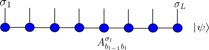
Figure 1: Graphical representation of matrix product state (MPS).

In order to obtain the ground state $|\psi_{0}\rangle$, one needs to find the MPS that minimizes the following equation

$$E=\frac{\langle\psi|\hat{H}|\psi\rangle}{\langle\psi|\psi\rangle}.$$ (7)

The most efficient way of doing this is in a variational approach by minimizing $E$ over MPS family

$$\min_{|\psi\rangle\in MPS}\left\{\langle\psi|\hat{H}|\psi\rangle-\lambda\langle\psi|\psi\rangle\right\}.$$ (8)

Ideally, the minimization should be done simultaneously over all the coefficients of all tensors. However, this is quite difficult and inefficient to implement. Following the original proceduredmrg_white1 ; dmrg_white2 , the strategy of DMRG that we use here is to minimize two tensors each time while keeping others fixed. Then, we move to another pair of tensors and repeat the procedure until convergence. In detail, defined $D^{\sigma_{l}\sigma_{l+1}}_{\alpha\beta}=\sum_{\gamma}A^{\sigma_{l}}_{\alpha,\gamma}A^{\sigma_{l+1}}_{\gamma,\beta}$ as the contraction of the two unfixed tensors. Then the minimization is written as

$$\min_{|\psi\rangle\in MPS}\left\{\langle\psi|\hat{H}|\psi\rangle-\lambda\langle\psi|\psi\rangle\right\}\rightarrow\\ \min_{D}\left\{D^{\dagger}\hat{H}_{eff}D-\lambda D^{\dagger}\hat{N}D\right\}.$$ (9)

$\hat{H}_{eff}$ and $\hat{N}$ correspond to $\langle\psi|\hat{H}|\psi\rangle$ and $\langle\psi|\psi\rangle$ without $D$ and $D^{\dagger}$, respectively. The term $-\lambda\langle\psi|\psi\rangle$ is introduced to make all eigenvalues negative, so that MPS is generated to converge to the ground state. By considering $D$ as a vector, the minimization becomes

$$\frac{\partial}{\partial D^{\dagger}}\left\{D^{\dagger}\hat{H}_{eff}D-\lambda D^{\dagger}\hat{N}D\right\}=0.$$ (10)

To proceed, we introduce two vectors

$$|\alpha\rangle = \sum_{\sigma_{1}\ldots\sigma_{l-1}}\left(A^{\sigma_{1}}\ldots A^{\sigma_{l-1}}\right)_{1,\alpha}|\sigma_{1}\ldots\sigma_{l-1}\rangle,$$ (11)

$$|\beta\rangle = \sum_{\sigma_{l+2}\ldots\sigma_{N}}\left(A^{\sigma_{l+2}}\ldots A^{\sigma_{N}}\right)_{\beta,1}|\sigma_{l+2}\ldots\sigma_{N}\rangle.$$ (12)

Then the state $|\psi\rangle$ can be written as follows

$$|\psi\rangle=\sum_{\sigma_{l}\sigma_{l+1}\alpha\beta}D^{\sigma_{l}\sigma_{l+1}}_{\alpha\beta}|\alpha\sigma_{l}\sigma_{l+1}\beta\rangle.$$ (13)

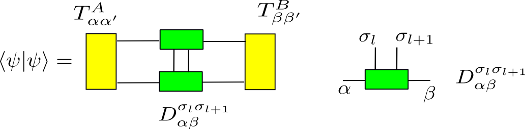
Figure 2: Graphical representation of $\langle\psi|\psi\rangle$ through the 2-rank tensors $T^{A}$ and $T^{B}$.

Let us first consider the overlap $\langle\psi|\psi\rangle$. As shown in Fig. 2, we use the Eq. (13)

$$\langle\psi|\psi\rangle=\sum_{\sigma_{l}\sigma_{l+1}}\sum_{\alpha\alpha^{\prime}}\sum_{\beta\beta^{\prime}}T^{A}_{\alpha\alpha^{\prime}}D^{\sigma_{l}\sigma_{l+1}}_{\alpha\beta}{D^{\sigma_{l}\sigma_{l+1}}_{\alpha^{\prime}\beta^{\prime}}}^{\dagger}T^{B}_{\beta\beta^{\prime}},$$ (14)

where $T^{A}_{\alpha\alpha^{\prime}}$ and $T^{B}_{\beta\beta^{\prime}}$ are

$$T^{A}_{\alpha\alpha^{\prime}} = \sum_{\sigma_{1}\ldots\sigma_{l-1}}\left({A^{\sigma_{l-1}}}^{\dagger}\ldots{A^{\sigma_{1}}}^{\dagger}A^{\sigma_{1}}\ldots A^{\sigma_{l-1}}\right)_{\alpha\alpha^{\prime}},$$ (15)

$$T^{B}_{\beta\beta^{\prime}} = \sum_{\sigma_{l+2}\ldots\sigma_{N}}\left(A^{\sigma_{l+2}}\ldots A^{\sigma_{N}}{A^{\sigma_{N}}}^{\dagger}\ldots{A^{\sigma_{l+2}}}^{\dagger}\right)_{\beta\beta^{\prime}}.$$ (16)

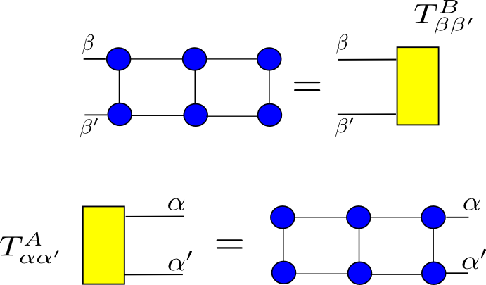
Figure 3: Graphical representation of the matrices $T^{A}$ and $T^{B}$ that contain the contraction.

The tensor $\hat{T}^{A}$ ($\hat{T}^{B}$) contains all the contraction of tensors of MPS from site $1$ to site $l-1$ ($l+2$ to $L$) (see Fig. 3). If the basis from the site $1$ to $l-1$ are left-orthogonal and the basis from $l+1$ to $N$ are right-orthogonal, we simply have

$$T^{A}_{\alpha\alpha^{\prime}}=\delta_{\alpha\alpha^{\prime}},\quad T^{B}_{\beta\beta^{\prime}}=\delta_{\beta\beta^{\prime}}.$$ (17)

We will show below that such left- and right- orthogonal conditions are automatically fulfilled in DMRG.

Let us now consider the quantity $\langle\psi|\hat{H}|\psi\rangle$. Assume that we can write $\hat{H}$ in a matrix product operator (MPO) CDV08 ; ND13 ; IPM (Fig. 4), i.e.,

$$\hat{H}=\hat{W}^{[1]}_{1,b_{1}}\hat{W}^{[2]}_{b_{1},b_{2}}\ldots\hat{W}^{[L]}_{b_{L-1},1},$$ (18)

where $\hat{W}^{[l]}=\sum_{\sigma_{l}\sigma^{\prime}_{l}}W^{\sigma_{l}\sigma^{\prime}_{l}}|\sigma_{l}\rangle\langle\sigma^{\prime}_{l}|$ is defined in a local Hilbert space.

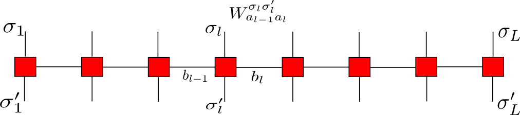
Figure 4: Matrix product operator representation of $\hat{H}$. In each site is defined an 4-rank tensor $\hat{W}^{\sigma_{l}\sigma^{\prime}_{l}}_{a_{l-1}a_{l}}$.

The $\langle\psi|\hat{H}|\psi\rangle$ is described in the tensor network in the Fig. 5 that containing the contraction between two MPS and the MPO. Therefore, one has

$$\langle\psi|\hat{H}|\psi\rangle=\sum_{\sigma_{l}\sigma_{l+1}\alpha\beta}\sum_{\sigma^{\prime}_{l}\sigma^{\prime}_{l+1}\alpha^{\prime}\beta^{\prime}}{D^{\sigma_{l}\sigma_{l+1}}_{\alpha\beta}}^{\dagger}D^{\sigma^{\prime}_{l}\sigma^{\prime}_{l+1}}_{\alpha^{\prime}\beta^{\prime}}\cdot\\ \langle\alpha\sigma_{l}\sigma_{l+1}\beta|\hat{H}|\alpha^{\prime}\sigma^{\prime}_{l}\sigma^{\prime}_{l+1}\beta^{\prime}\rangle.$$ (19)

Let us now look at the matrix elements $\langle\alpha\sigma_{l}\sigma_{l+1}\beta|\hat{H}|\alpha^{\prime}\sigma^{\prime}_{l}\sigma^{\prime}_{l+1}\beta^{\prime}\rangle$ using the MPO representation of Hamiltonian $H$

$$\langle\alpha\sigma_{l}\sigma_{l+1}\beta|\hat{H}|\alpha^{\prime}\sigma^{\prime}_{l}\sigma^{\prime}_{l+1}\beta^{\prime}\rangle=\sum_{\sigma\sigma^{\prime}}W^{\sigma_{1}\sigma^{\prime}_{1}}\ldots W^{\sigma_{L}\sigma^{\prime}_{L}}\\ \cdot\langle\alpha\sigma_{l}\sigma_{l+1}\beta|\sigma_{1}\ldots\sigma_{L}\rangle\langle\sigma^{\prime}_{1}\ldots\sigma^{\prime}_{L}|\alpha^{\prime}\sigma^{\prime}_{l}\sigma^{\prime}_{l+1}\beta^{\prime}\rangle.$$ (20)

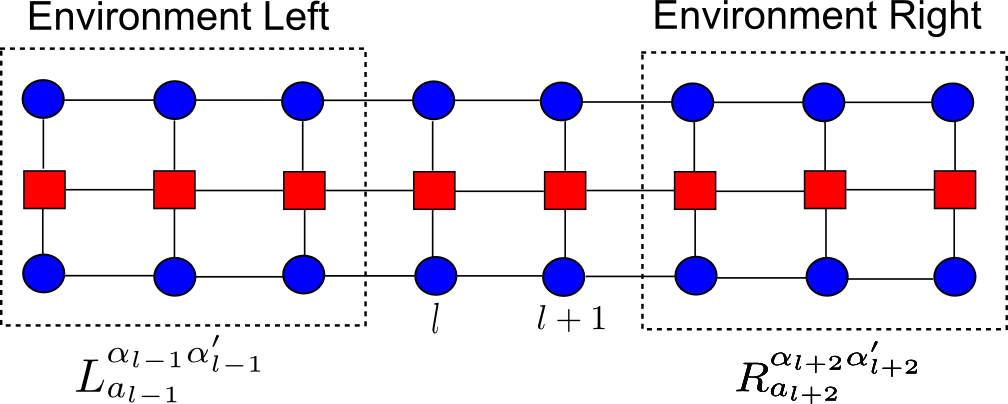
Figure 5: Tensor network represented the quantity $\langle\psi|\hat{H}|\psi\rangle$.

Using the equations (11) and (12), we can evaluate the scalar product in the previous equation

$$\langle\alpha\sigma_{l}\sigma_{l+1}\beta|\sigma^{\prime}_{1}\cdots\sigma^{\prime}_{L}\rangle=\left({A^{\sigma_{1}}}^{\dagger}\cdots{A^{\sigma_{l-1}}}^{\dagger}\right)_{1,\alpha}\\ \cdot\left({A^{\sigma_{l+2}}}^{\dagger}\cdots{A^{\sigma_{L}}}^{\dagger}\right)_{\beta,1},$$ (21)

$$\langle\sigma^{\prime}_{1}\cdots\sigma^{\prime}_{L}|\alpha^{\prime}\sigma^{\prime}_{l}\sigma^{\prime}_{l+1}\beta^{\prime}\rangle=\left(A^{\sigma^{\prime}_{1}}\cdots A^{\sigma^{\prime}_{l-1}}\right)_{1,\alpha^{\prime}}\\ \cdot\left(A^{\sigma^{\prime}_{l+2}}\cdots A^{\sigma^{\prime}_{L}}\right)_{\beta^{\prime},1}.$$ (22)

Define the tensors $L$ and $R$ that contain the contracted left and right halves as (see Fig. 6)

$${L}^{\alpha\alpha^{\prime}}_{a_{l-1}}=\left\{\sum_{\sigma_{1}\sigma^{\prime}_{1}}{A^{\sigma_{1}}_{1,b_{1}}}^{\dagger}W^{\sigma_{1}\sigma^{\prime}_{1}}_{1,a_{1}}A^{\sigma^{\prime}_{1}}_{1,b^{\prime}_{1}}\right\}\cdots\\ \cdots\left\{\sum_{\sigma_{l-1}\sigma^{\prime}_{l-1}}{A^{\sigma_{l-1}}_{b_{l-2},b_{l-1}}}^{\dagger}W^{\sigma_{l-1}\sigma^{\prime}_{l-1}}_{a_{l-2},a_{l-1}}A^{\sigma^{\prime}_{l-1}}_{b^{\prime}_{l-2},b^{\prime}_{l-1}}\right\},$$ (23)

$${R}^{\beta\beta^{\prime}}_{a_{l+1}}=\left\{\sum_{\sigma_{l+2}\sigma^{\prime}_{l+2}}{A^{\sigma_{l+2}}}^{\dagger}W^{\sigma_{l+2}\sigma^{\prime}_{l+2}}_{a_{l+1}a_{l+2}}A^{\sigma^{\prime}_{l+2}}\right\}\cdots\\ \cdots\left\{\sum_{\sigma_{L}\sigma^{\prime}_{L}}{A^{\sigma_{L}}_{b_{l+1},b_{l+2}}}^{\dagger}W^{\sigma_{L}\sigma^{\prime}_{L}}_{a_{L-1}1}A^{\sigma^{\prime}_{L}}_{b^{\prime}_{l+1},b^{\prime}_{l+2}}\right\}.$$ (24)

Through the Eqs. (23) and (24), we obtain

$$\langle\alpha\sigma_{l}\sigma_{l+1}\beta|\hat{H}|\alpha^{\prime}\sigma^{\prime}_{l}\sigma^{\prime}_{l+1}\beta^{\prime}\rangle=\\ =\sum_{a_{l-1}a_{l}a_{l+1}}{L}^{\alpha\alpha^{\prime}}_{a_{l-1}}W^{\sigma_{l}\sigma^{\prime}_{l}}_{a_{l-1}a_{l}}W^{\sigma_{l+1}\sigma^{\prime}_{l+1}}_{a_{l}a_{l+1}}{R}^{\beta\beta^{\prime}}_{a_{l}}.$$ (25)

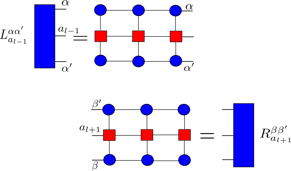
Figure 6: Graphical representation of environment left $L$ and right $R$, where $L$ contain the contracted left part while $R$ contain the contracted right part of network.

Now we can immediately write $\langle\psi|\hat{H}|\psi\rangle$ as

$$\langle\psi|\hat{H}|\psi\rangle=\sum_{\alpha\alpha^{\prime}}\sum_{\beta\beta^{\prime}}\sum_{\sigma_{l}\sigma^{\prime}_{l}}\sum_{\sigma_{l+1}\sigma^{\prime}_{l+1}}{D^{\sigma_{l}\sigma_{l+1}}_{\alpha\beta}}^{\dagger}D^{\sigma_{l}\sigma_{l+1}}_{\alpha^{\prime}\beta^{\prime}}\cdot\\ \cdot{L}^{\alpha\alpha^{\prime}}_{a_{l-1}}W^{\sigma_{l}\sigma^{\prime}_{l}}_{a_{l-1}a_{l}}W^{\sigma_{l+1}\sigma^{\prime}_{l+1}}_{a_{l}a_{l+1}}{R}^{\beta\beta^{\prime}}_{a_{l}},$$ (26)

and rewrite Eq. (10) as

$$\sum_{\alpha^{\prime}\beta^{\prime}}\sum_{\sigma_{l}\sigma^{\prime}_{l}}\sum_{\sigma_{l+1}\sigma^{\prime}_{l+1}}L^{\alpha\alpha^{\prime}}_{a_{l-1}}W^{\sigma_{l}\sigma^{\prime}_{l}}_{a_{l-1}a_{l}}W^{\sigma_{l+1}\sigma^{\prime}_{l+1}}_{a_{l}a_{l+1}}R^{\beta\beta^{\prime}}_{a_{l+1}}D^{\sigma_{l}\sigma^{\prime}_{l}}_{\alpha^{\prime}\beta^{\prime}}\\ -\lambda\sum_{\alpha^{\prime}\beta}T^{A}_{\alpha\alpha^{\prime}}T^{B}_{\beta\beta^{\prime}}D^{\sigma_{l}\sigma_{l+1}}_{\alpha\beta}=0.$$ (27)

The matrices $H_{eff}$ (see Fig. 7) and $N$ simply are

$$H_{eff}=\sum_{a_{l-1}a_{l}a_{l+1}}L^{\alpha\alpha^{\prime}}_{a_{l-1}}W^{\sigma_{l}\sigma^{\prime}_{l}}_{a_{l-1}a_{l}}W^{\sigma_{l+1}\sigma^{\prime}_{l+1}}_{a_{l}a_{l+1}}R^{\beta\beta^{\prime}}_{a_{l+1}},$$ (28)

$$N=T^{A}_{\alpha\alpha^{\prime}}T^{B}_{\beta\beta^{\prime}}.$$ (29)

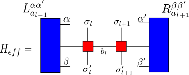
Figure 7: Graphical representation of effective Hamiltonian $H_{eff}$ defined in equation (28).

Using the expressions above, the minimization problem becomes

$$H_{eff}D-\lambda ND=0.$$ (30)

After solving $D^{\sigma_{l}\sigma_{l+1}}_{\alpha\beta}$, we update $A^{\sigma_{l}}_{\alpha\beta}$ by performing a SVD

$$D^{\sigma_{l}\sigma_{l+1}}_{\alpha\beta}=\sum_{\rho}U_{\sigma_{l}\alpha,\rho}S_{\rho}V_{\rho,\sigma_{l+1}\beta}.$$ (31)

Take only the $\chi$ largest singular vectors in $U$ as the new tensor $A^{\sigma_{l}}_{\alpha\rho}$, i.e., $A^{\sigma_{l}}_{\alpha\rho}=U_{\sigma_{l}\alpha,\rho}$ when sweeping from left to right, and take the $\chi$ largest singular vectors in $V$ as the new tensor $A^{\sigma_{l+1}}_{\rho,\beta}$ when sweeping from right to left. In this way, the left and right orthogonal conditions of the MPS are automatically fulfilled.

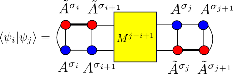
Figure 8: Graphical representation of the overlap $\langle\psi_{i}|\psi_{j}\rangle$ represented in the equation (34).

Specifically speaking, a left-to-right (or right-to-left) sweep consists of the following steps:

• Start with a random initial MPS and transform it in the right orthogonal form.

• Optimize the tensor $D^{\sigma_{i}\sigma_{i+1}}$: construct the environment $L$ and $R$ and solve the standard eigenvalue problem:

  $$H_{eff}D-\lambda D=0$$ (32)

• Carry out an SVD of $D^{\sigma_{i}\sigma_{i+1}}$ and update the tensor $A^{\sigma_{i}}$.

• Repeat the same operations for every site until reaching the preset convergence:

  $$\langle\psi|\hat{H}^{2}|\psi\rangle-\left(\langle\psi|\hat{H}|\psi\rangle\right)^{2}\rightarrow 0.$$ (33)

To analyse the computational cost we have to take special care to ensure optimal ordering of multiplications when dealing with each eigensolver given by (32). The problem is to contract $L_{i-1}W_{i}W_{i+1}R_{i+2}D^{\sigma_{i}\sigma_{i+1}}$, with $L_{i-1}$ $R_{i+2}\in(\chi,\chi_{W},\chi)$, $W_{i}\in(d,\chi_{W},d\chi_{W})$ and $D^{\sigma_{i}\sigma_{i+1}}\in(\chi,d,\chi)$. The optimal ordering should be $(((L_{i-1}D^{\sigma_{i}\sigma_{i+1}})W_{i}W_{i+1})R_{i+2}$, and in the way, one has to

• Contract $L_{i-1}$ and $D^{\sigma_{i}\sigma_{i+1}}$ over the left MPS bond at a cost $O(\chi^{3}\cdot\chi_{W}\cdot d^{2})$.

• Multiply with $W_{i}W_{i+1}$ over the physical bond of $D^{ii+1}$ at a cost $O(\chi^{2}\cdot\chi_{W}^{2}\cdot d^{4})$.

• Contract with $R_{i+2}$ over the right MPO and MPS bond at a cost $O(\chi^{3}\cdot d^{2}\cdot\chi_{W})$

The total cost of this procedure to apply $\hat{H}$ to $|\psi\rangle$ is $O(\chi^{3}\cdot\chi_{W}\cdot d^{2}+\chi^{2}\cdot\chi_{W}^{2}\cdot d^{4}+\chi^{3}\cdot d^{2}\cdot\chi_{W})$.

III Subspace Expansion

In the following, we develop a second-order perturbation theory for DMRG. Note that from the orthogonality that the contribution of the first-order term is zero. This optimization permits the recovery of some of the lost information due to the truncation in the SVD of $D^{\sigma_{i}\sigma_{i+1}}$, and reach a better approximation of the ground state. In last section, we have shown how DMRG works and where its error comes from. To reduce the error, we define a new orthogonal basis $\{|\psi_{i}\rangle\}$, whose elements have the MPS form. We put an impurity bond in each $\{|\psi_{i}\rangle\}$ so that it is orthogonal to the ground state obtained by DMRG. To define this impurity bond (e.g. between the $i$-th and ($i+1$)-th sites), we consider the SVD of $D^{\sigma_{i}\sigma_{i+1}}$ and the tensor $\tilde{A}^{\sigma_{i}}$ as the second $\chi$ largest singular vectors. Thus, $\tilde{A}^{\sigma_{i}}$ is orthogonal to the tensor $A^{\sigma_{i}}$ in the original MPS.

By introducing one impurity in different bonds of $|\psi_{0}\rangle$, we can define a new basis $\{|\psi_{i}\rangle\}$. Since both are in orthogonal form, one has

$$\langle\psi_{i}|\psi_{j}\rangle=\sum A^{\sigma_{i}}\left(\tilde{A}^{\sigma_{i}}\right)^{\dagger}A^{\sigma_{i+1}}\left(\tilde{A}^{\sigma_{i+1}}\right)^{\dagger}M^{j-i+1}\\ \tilde{A}^{\sigma_{j}}\left(A^{\sigma_{j}}\right)^{\dagger}\tilde{A}^{\sigma_{j+1}}\left(A^{\sigma_{j+1}}\right)^{\dagger},$$ (34)

where $M$ is the transfer matrix of the overlap $\langle\psi_{i}|\psi_{j}\rangle$ (see Fig. 8). Thus, $|\psi_{i}\rangle$ and $|\psi_{j}\rangle$ are orthogonal to each other for $i\neq j$.

Now one can define the perturbed Hamiltonian $\hat{\mathcal{H}}$ with $\{|\psi_{i}\rangle\}$ ($i=0,1,\cdots$). Note that $|\psi_{0}\rangle$ is the ground state by the original DMRG. The matrix elements of $\hat{\mathcal{H}}$ are defined as

$$\mathcal{H}_{ij}=\langle\psi_{i}|\hat{\mathcal{H}}|\psi_{j}\rangle$$ (35)

and form the matrix $\mathcal{H}$. The ground state energy is calculated as

$$\tilde{E}_{0}=\frac{\langle\tilde{\psi}_{0}|\hat{\mathcal{H}}|\tilde{\psi}_{0}\rangle}{\langle\tilde{\psi}_{0}|\tilde{\psi}_{0}\rangle}$$ (36)

where $|\tilde{\psi}_{0}\rangle$ is defined as the combination of $\{|\psi_{i}\rangle\}$

$$|\tilde{\psi}_{0}\rangle=\sum_{j}\Psi_{j}|\psi_{j}\rangle,$$ (37)

where $\Psi_{j}$ are the coordinates of the dominant eigenvector of $\hat{\mathcal{H}}$. By using that the basis $\{|\psi_{i}\rangle\}$, the perturbed ground state energy is simply obtained as

$$\tilde{E}_{0}=\sum_{ij}\Psi^{\dagger}_{j}\mathcal{H}_{ij}\Psi_{j}.$$ (38)

IV Perturbation Theory DMRG

Now we explain how to implement the PT-DMRG in practice. Using the notation introduced above, the steps follow mostly the standard DMRG. In an outermost loop, the update sweeps over the system from left to right and right to left until the preset convergence is reached. The inner loop sweeps over the system, iterating over and updating the tensors on each site sequentially. Each local update during a left to right sweep consists of the following steps:

• Perform the standard DMRG to obtain the ground state MPS $|\psi_{0}\rangle$ (which is assumed in the right-orthogonal form).

• From left to right, calculate $D^{\sigma_{i}\sigma_{i+1}}$ and perform SVD for each $i$; Keep the second $\chi$ largest left and right singular vectors as $\tilde{A}^{\sigma_{i}}$ and $\tilde{A}^{\sigma_{i+1}}$, respectively.

• Construct the orthogonal basis $\{|\psi_{i}\rangle\}$ for by putting an impurity $\tilde{A}^{\sigma_{i}}$ in different bonds.

• Construct the perturbed Hamiltonian $\hat{\mathcal{H}}$ according to Eq. (35) and calculate its dominant eigenvector $\Psi$.

• Calculate the perturbed ground state of the systems as

  $$|\tilde{\psi}_{0}\rangle=\sum_{i=1}^{N}\Psi_{i}|\psi_{i}\rangle.$$ (39)

As regards the computational cost, in addition, we need to consider the diagonalization of $\hat{\mathcal{H}}$ in the subspace. This cost is $O(N^{3})$ where $N$ is the number of the perturbed basis. Therefore the full cost is $\chi^{3}d\chi_{W}+O(\chi^{2})+O(N^{3})$, which makes it quite expensive. But the diagonal and first row/column of $\cal{H}$ can be obtained easily during the final DMRG sweep itself, which makes it much more practical.

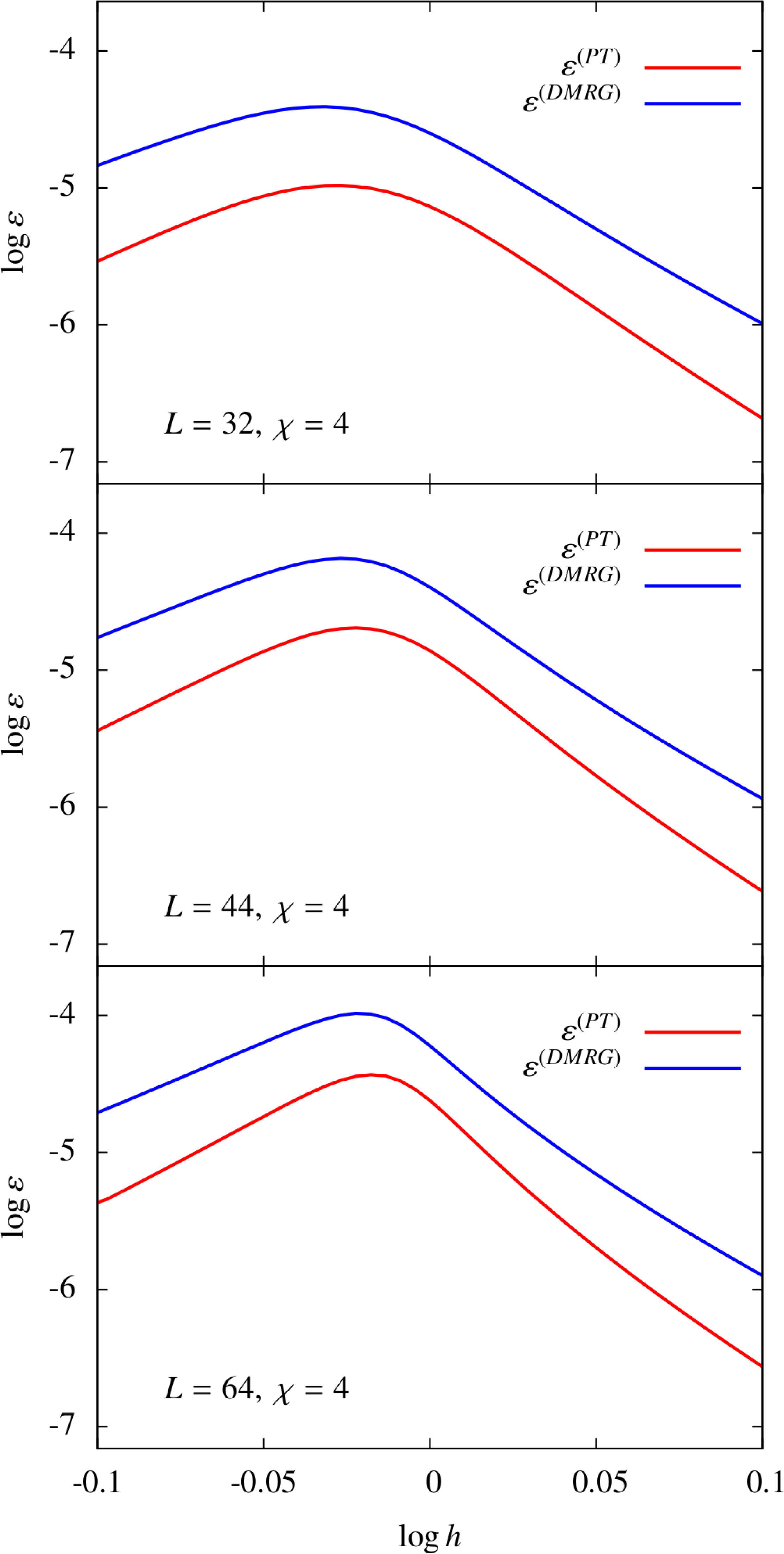
Figure 9: The error $\varepsilon$ of 1D Ising model on $32,44,64$ chain with open boundary condition as a function of $h$. The error of PT-DMRG method with bond dimension $\chi=4$ is more than $O(10)$ time smaller compared with the error of standard DMRG.

V Numerical Results

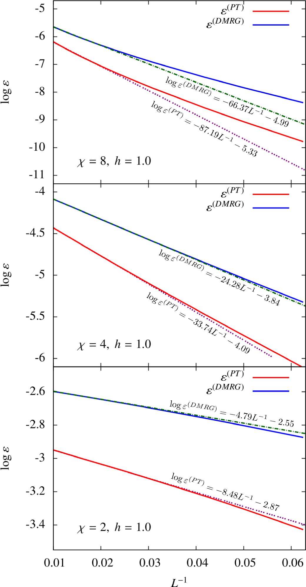
Figure 10: The error $\varepsilon$ of 1D Ising model as a function of length in the quantum phase transition $h=1.0$, for different values of $\chi=2,4,8$. We show that the error PT-DMRG is much smaller. The PT-DMRG gives a systematic improvement of accuracy.

Quantum Transverse Ising Model

To illustrate our method we study the 1D spin-half quantum Ising model in a transverse field, especially near the quantum phase transition. The Hamiltonian reads

$$\hat{H}=-J\sum_{i=1}^{L}\hat{\sigma}^{x}_{i}\hat{\sigma}^{x}_{i+1}+h\sum_{i=1}^{L}\hat{\sigma}^{z}_{i}.$$ (40)

In the infinite case, a quantum phase transition occurs at $h/J=1$. The system for $h/J>1.0$ is in a paramagnetic phase with an order parameter $\langle S^{x}\rangle\neq 0$, and in a ferromagnetic phase for $h/J<1.0$ with an order parameter $\langle S^{z}\rangle\neq 0$. At the critical point, both order parameters go to zero. We set $J=1$ as the energy scale.

In the numerical simulations, we considered a finite-size system with open boundary condition with the length $L=16\sim 128$. To benchmark PT-DMRG, we compute the ground state energies of DMRG and PT-DMRG with the same bond dimension $\chi$, and compare with the (quasi-exact) result from the DMRG with sufficiently large $\chi=100\sim 400$ (note $\chi$ for quasi-exact calculations changes according with the length of the chain, in other words the entanglement). The error is defined as

$$\varepsilon=\frac{E_{0}-\langle\psi|\hat{H}|\psi\rangle}{E_{0}},$$ (41)

with $E_{0}$ the energy from the quasi-exact DMRG.

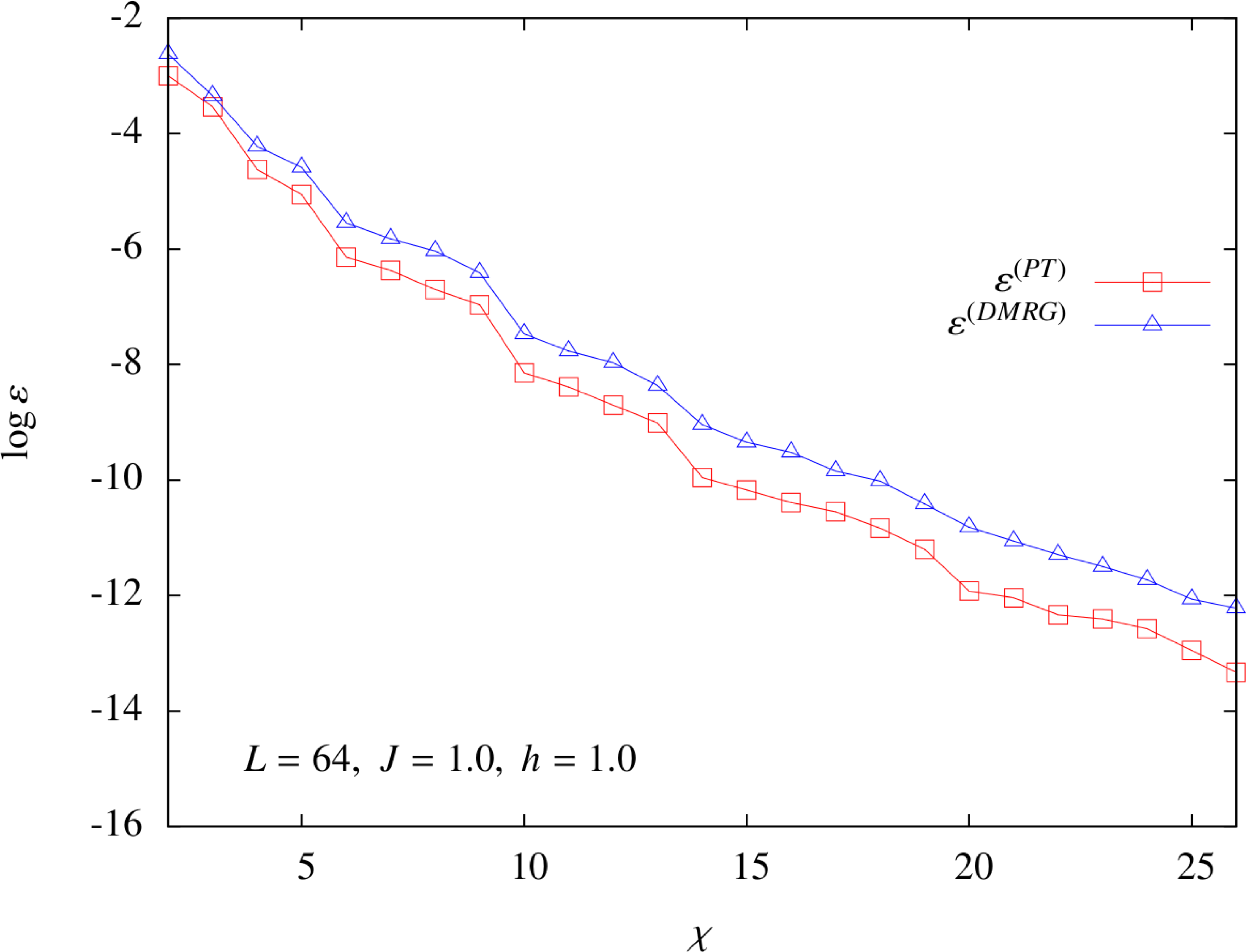
Figure 11: The error $\varepsilon$ of 1D Ising model versus of $\chi$ in the quantum phase transition $h=1.0$ for $L=64$. We show how the error of PT-DMRG decrease faster than the error of the standard DMRG.

The Fig. 9 shows the error with $L=32,44,64$ versus magnetic field $h$. We compare the results of the conventional DMRG and PT-DMRG for $\chi=2,4,8$. Near to the phase transition, the error of PT-DMRG is more than $O(10)$ times smaller compared with the error of the conventional DMRG with the same $\chi$. Our simulations suggest that through PT-DMRG, we are able to retrieve the leading term of the lost information with the truncations in the SVD.

In Fig. 10, we show the error against $L^{-1}$ for $h=1$ (critical point). The results show that the error increase both linearly with $L^{-1}$ for DMRG and PT-DMRG, indicating a systematic improvement of the accuracy for moderate values of $L$. For the thermodynamic limit the error of PT-DMRG scales as $\sqrt{L^{-1}}$, for reasons explained below.

In Fig. 11, we show the error against $\chi$ for $h=1$ (phase transition) and for $L=64$. The results show that the error decrease with bond dimension $\chi$ for DMRG and PT-DMRG. The error of PT-DMRG decreases faster than that of standard DMRG. This shows considerable improvement of the accuracy for any value of bond dimension $\chi$ near the phase transition.

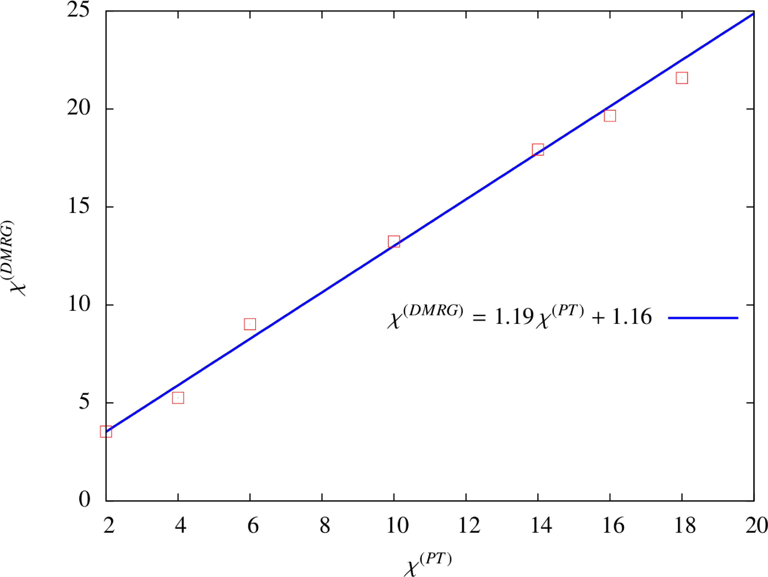
Figure 12: The plot is the fit between $\chi^{(DMRG)}$ versus of $\chi^{(PT)}$ of 1D Ising model in the quantum phase transition $h=1.0$ for $L=64$. We show how the PT-DMRG needs smaller bond dimension $\chi$ than DMRG.

To see more clearly the improvement of the efficiency of PT-DMRG, we study the correspondence between the bond dimension cut-off $\chi^{(DMRG)}$ of the standard DMRG and that of PT-DMRG $\chi^{(PT)}$. As shown in Fig. 12, each pair of $\chi^{(DMRG)}$ and $\chi^{(PT)}$ given by the data points approximately have the same precision. In detail, to determine $\chi^{(DMRG)}$ for a given $\chi^{(PT)}$, we first find two $\chi$’s with DMRG, where the precision of one $\chi$ is higher than the precision of PT-DMRG with $\chi^{(PT)}$, and the other is lower. Then, we do a fit to find $\chi^{(DMRG)}$, which is an fraction between these two $\chi$’s.

We choose $h=1$ and $L=64$. The results show that with each $\chi^{(PT)}$ in PT-DMRG, we need a larger bond dimension cut-off (i.e. keep more states) in DMRG to reach the same precision. We also find a linear relation between $\chi^{(PT)}$ and $\chi^{(DMRG)}$ as

$$\chi^{(DMRG)}=1.19\chi^{(PT)}+1.16.$$ (42)

Since the computational cost an MPS takes scales as $\sim\chi^{2}$ (2 is the number of the virtual bond in each local tensor of MPS), such a linear relation suggests that the larger $\chi$ one uses, the more computational resource one can save by using PT-DMRG.

Heisenberg Model

We study also the 1D spin-half quantum Heisenberg model, where the Hamiltonian reads

$$\hat{H}=-J\sum_{i=1}^{L}(\hat{\sigma}^{x}_{i}\hat{\sigma}^{x}_{i+1}+\hat{\sigma}^{y}_{i}\hat{\sigma}^{y}_{i+1}+\hat{\sigma}^{z}_{i}\hat{\sigma}^{z}_{i+1}).$$ (43)

We take $J=1$ as energy scale.

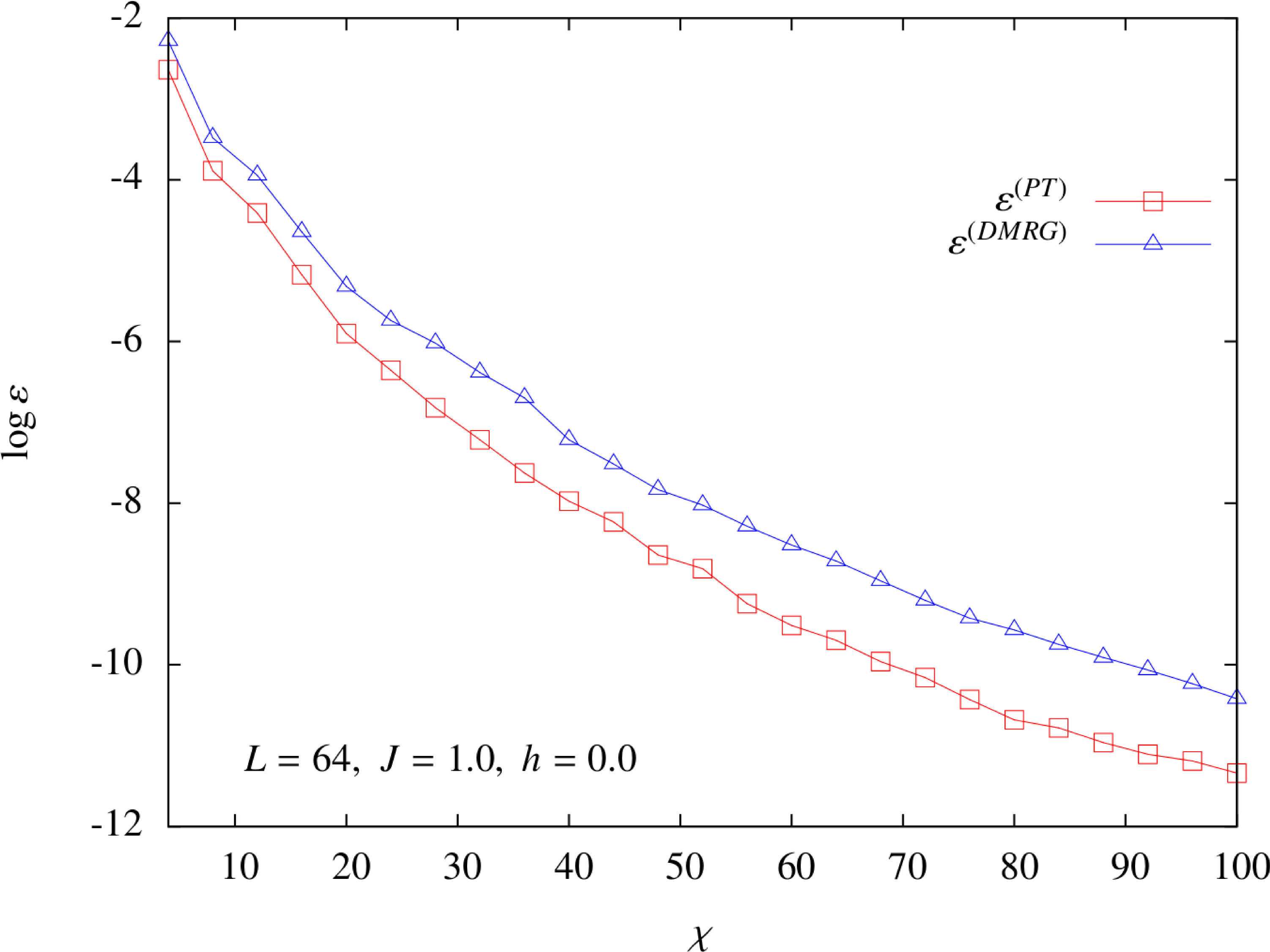
Figure 13: The error $\varepsilon$ of 1D Heisenberg model versus of $\chi$ in the quantum phase transition $h=0.0$ for $L=64$. We show how the error of PT-DMRG decrease faster than the error of the standard DMRG.

In Fig. 13, we show the error against $\chi$ for $L=64$. The results show that the error decrease with bond dimension $\chi$ for DMRG and PT-DMRG. Amazingly, the error of PT-DMRG decreases faster than that of standard DMRG. This shows considerable improvement of the accuracy for any value of bond dimension $\chi$.

In Fig. 14, we show the fit of $\chi^{(DMRG)}$ against $\chi^{(PT)}$ for $L=64$. Again, a linear relation is found between $\chi^{(PT)}$ and $\chi^{(DMRG)}$ as

$$\chi^{(DMRG)}=1.32\chi^{(PT)}+0.23.$$ (44)

Especially, the slope is larger than that in the quantum Ising model, which implies a more significant improvement of efficiency when calculating Heisenberg chain with a large bond dimension cut-off.

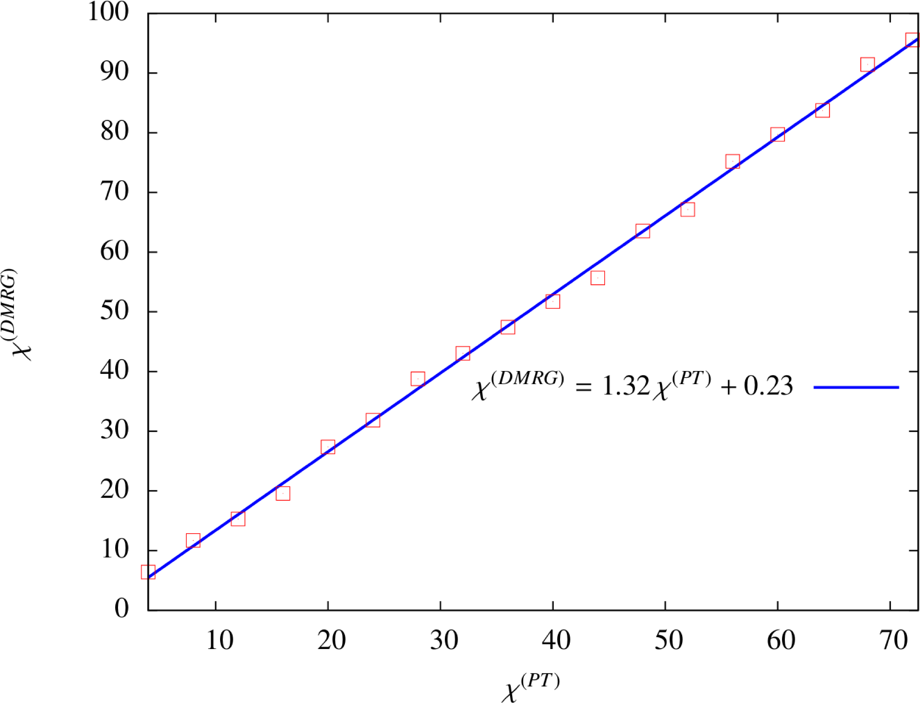
Figure 14: The plot is the fit between $\chi^{(DMRG)}$ versus of $\chi^{(PT)}$ of 1D Heisenberg model in the quantum phase transition $h=0.0$ for $L=64$. We show how the PT-DMRG needs smaller bond dimension $\chi$ than DMRG.

VI Thermodynamic Limit

In the following, we explore a second order perturbation theory for DRMG in the thermodynamic limit. In the previous section we showed that the error scaling of PT-DMRG is linear in $L^{-1}$ for moderate $L$. Now if $L$ approach to infinity we have that the scaling law is $1/\sqrt{L}$.

We focus on the results first in the Fig. 10. If we extend the results to larger $L$ we can see a changing in behaviour for large $L$ limit, the error in the energy per site becomes exactly equal to that of conventional DMRG.

We can understand that from looking at how the PT-DMRG approaches the thermodynamic limit. The off-diagonal matrix elements of effective Hamiltonian $\mathcal{H}_{ij}$ for $|i-j|>1$ decay exponentially quickly, so it really only needs a few of them. For the Ising model $\mathcal{H}_{i,i+2}$ is already $O(10^{-6})$, so this gives no improvement over the old style of calculating just the diagonal part and the overlap with the ground state. In the large $L$ limit, the effective Hamiltonian $\mathcal{H}_{ij}$ can be well-approximated by:

$$\mathcal{H}=\begin{bmatrix}a&b&b&b&b&\cdots\\ b&c&0&0&0&\cdots\\ b&0&c&0&0&\cdots\\ b&0&0&c&0&\cdots\\ \vdots&\vdots&\vdots&\vdots&\vdots&\ddots\\ \end{bmatrix},$$ (45)

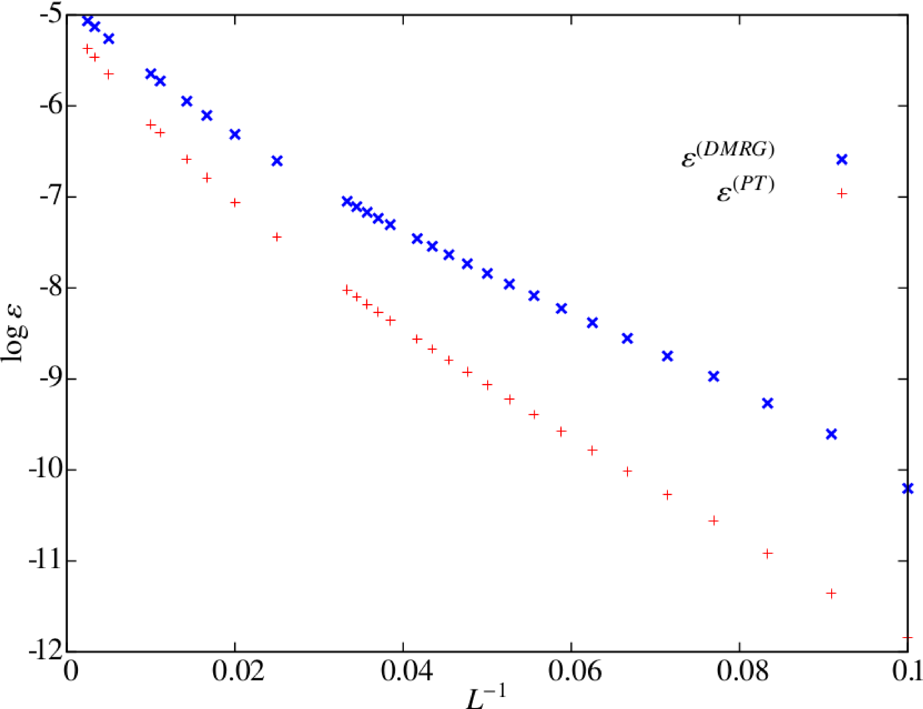
Figure 15: The error $\varepsilon$ of 1D Ising model as a function of length in the quantum phase transition h = 1.0, for $\chi=8$. We show that the error PT-DMRG In the large $L$ limit doesn’t give a systematic improvement of accuracy.

where the non-zero elements are $a=E_{0}$ at the top-left (the energy of the original ground state), a series of $L$ entries along the top row and left column which is $b=\langle\psi_{i}|H|\psi_{0}\rangle$ (assumed independent of i in the large $L$ limit), and the diagonal entries $c=\langle\psi_{i}|H|\psi_{i}\rangle$ independent of $i$ in the large $L$ limit. $a$ and $c$ are extensive in the system size, but $c$ has a constant offset because of the local perturbation. So we can set:

$$a=E_{0}\times L\qquad c=E_{0}\times L+q,$$ (46)

where $q$ is the energy of the perturbation. It is possible to determine the eigenvalues of this matrix as a function of L, which is

$$E=(E_{0}\times L+\frac{q}{2})-\Delta,$$ (47)

where

$$\Delta^{2}=\frac{q^{2}}{4}+b^{2}L.$$ (48)

So we can see the origin now of the $1/\sqrt{(}L)$ behaviour. For large $L$ the energy per site scales as

$$\frac{E}{L}=E_{0}-\frac{|b|}{\sqrt{L}}+O(1/\sqrt{L}).$$ (49)

But in order to see the square root behaviour $b^{2}L>>q^{2}/4$, which for the ising model, requires L ¿ 650 (see Fig. 15 ). The plot in Fig. 10 is basically linearizing a square root in a region well away from the asymptotic large $L$ behaviour.

VII Summary and outlook

A simple and efficient numeric approach named PT-DMRG is proposed to largely improve the accuracy of the conventional DMRG. It gives a better approximation of ground state of strongly-correlated many-body systems by recovering the leading term of entanglement that is discarded in the truncations of DMRG. By using MPS representation, we introduce a set of orthogonal basis to define the perturbed Hamiltonian, whose ground state possesses a better precision than the traditional DMRG. In other words, we use the Schmidt numbers that are beyond the dimension cut-off to define the perturbation terms. By using the second order PT-DMRG, our numerical results obtained for the 1D quantum Ising model and Heisenberg model show a better accuracy reached by our PT-DMRG, where the precision of DMRG is shown to be improved significantly (around $O(10)$ times).

Our PT-DMRG provides a fundamental scheme that can be directly used for 2D DMRG algorithm. Such perturbation theory based on MPS can be generalized to other MPS or even TN algorithms, such as time-evolved block decimation. The generalization to higher-order perturbation theories is be explored in the future.

Finally, the perturbation theories can provide a fundamental scheme to study the power-low correlation. For example in the MERA the isometries can be used to define perturbed terms. The kernel space of each original isometry provides the tangent space in a natural way. So the perturbation idea may be useful in any state ansatz that gives a renormalization flow.

VIII Acknowledgements

This work was supported by ERC ADG OSYRIS, EQuaM (FP7/2007-2013 Grant No. 323714), Spanish MINECO (Severo Ochoa grant SEV-2015-0522), FOQUS (FIS2013-46768), Catalan AGAUR SGR 874, Fundació Cellex and EU FETPRO QUIOC, Marie Curie fellowship SQSNP 622939 FP7-MC-IIF.

References

- (1) S. Sachdev, Quantum Phase Transitions, 2nd ed. Cambridge University Press, Cambridge, (2011).
- (2) C. Lacroix, P. Mendels and F. Mila, Introduction to frustrated Magnetism, Springer, Heidelberg, (2011).
- (3) M. Lewenstein, A. Sanpera, and V. Ahufinger, Ultracold atoms in optical lattices: Simulating quantum many-body systems, Oxford University Press (2012).
- (4) C. Castelnovo, R. Moessner, and S. Sondhi, Spin Ice, Fractionalization, and Topological Order, Ann. Rev. Cond. Mat. Phys. 3, 35 (2012).
- (5) P. W. Anderson, The Resonating Valence Bond State in and Superconductivity, Science 235, 1196 (1987).
- (6) P. A. Lee, N. Nagaosa and X. G. Wen, Doping a Mott insulator: Physics of high-temperature superconductivity, Rev. Mod. Phys. 78, 17 (2006).
- (7) J. M. Kosterlitz and J. Thouless, Long range order and metastability in two dimensional solids and superfluids (Application of dislocation theory), Solid State Phys. 5, L124 (1972).
- (8) B. A. Bernevig and T. L. Hughes, Topological Insulators and Topological Superconductors, Princeton University Press (2013).
- (9) L. Balents, Spin liquids in frustrated magnets, Nature 464, 199-208 (2010).
- (10) A. Banerjee, C. A. Bridges, J. Q. Yan, A. A. Aczel, L. Li, M. B. Stone, G. E. Granroth, M. D. Lumsden, Y. Yiu, J. Knolle, S. Bhattacharjee, D. L. Kovrizhin, R. Moessner, D. A. Tennant, D. G. Mandrus and S. E. Nagler, Proximate Kitaev quantum spin liquid behaviour in a honeycomb magnet, Nat. Mat. doi:10.1038/nmat4604 (2016).
- (11) H. Bethe, On the theory of metals. I. Eigenvalues and eigenfunctions of the linear atom chain, Z. Phys. A 71, 205 (1931).
- (12) E. H. Lieb and F. Y. Wu, Absence of Mott Transition in an Exact Solution of the Short-Range, One-Band Model in One Dimension, Phys. Rev. Lett. 20, 1445 (1968).
- (13) F. H. L. Essler, H. Frahm, F. Göhmann, A. Klümper, and V. E. Körepin, The one-dimensional hubbard model, Cambridge University Press, (2005).
- (14) A. W. Sandvik, Computational Studies of Quantum Spin Systems, AIP Conf. Proc. 1297, 135 (2010).
- (15) M. Troyer and U. J. Wiese, Computational Complexity and Fundamental Limitations to Fermionic Quantum Monte Carlo Simulations, Phys. Rev. Lett. 94, 170201 (2005).
- (16) U. Schollwök, The density-matrix renormalization group in the age of matrix product states, Ann. Phys. 96, 326 (2011).
- (17) R. Orus, A Practical Introduction to Tensor Networks: Matrix Product States and Projected Entangled Pair States, Ann. Phys. 349, 117 C158 (2014).
- (18) J. Eisert, M. Cramer and M. B. Plenio, Area laws for the entanglement entropy, Rev. Mod. Phys. 82, 277 (2010).
- (19) G. Vidal, J. I. Latorre, E. Rico and A. Kitaev, Entanglement in Quantum Critical Phenomena, Phys. Rev. Lett. 90, 227902 (2003).
- (20) J. I. Latorre, E. Rico and G. Vidal, Ground state entanglement in quantum spin chains, Quant. Inf. Comp. 4, 48 (2004).
- (21) I. Peschel, M. Kaulke and O. Legeza, Density-matrix spectra for integrable models, Ann. Phys. (Leipzig) 8, 153 (1999).
- (22) J. D. Bekenstein, Black Holes and Entropy, Phys. Rev. D 7, 2333 (1973).
- (23) M. Srednicki, Entropy and area, Phys. Rev. Lett. 71, 666 (1993).
- (24) M. B. Plenio, J. Eisert, J. Dreissig and M. Cramer, Entropy, Entanglement, and Area: Analytical Results for Harmonic Lattice Systems, Phys. Rev. Lett. 94, 060503 (2005).
- (25) P. Calabrese and J. Cardy, Entanglement entropy and quantum field theory, J. Stat. Mech.: Theo. Exp. P06002, (2004).
- (26) U. Schollwöck, The density-matrix renormalization group, Rev. Mod. Phys. 77, 259 (2005).
- (27) K. A. Hallberg, New Trends in Density Matrix Renormalization, Adv. Phys. 55, 477 (2006).
- (28) S. R. White, Density matrix formulation for quantum renormalization groups, Phys. Rev. Lett. 69, 2863 (1992).
- (29) S. R. White, Density-matrix algorithms for quantum renormalization groups, Phys. Rev. B 48, 10345 (1993).
- (30) K. G. Wilson, The renormalization group: Critical phenomena and the Kondo problem, Rev. Mod. Phys. 47, 773 (1975).
- (31) S. Östlund and S. Rommer, Thermodynamic Limit of Density Matrix Renormalization, Phys. Rev. Lett. 75, 3537 (1995).
- (32) F. Verstraete, D. Porras, and J. I. Cirac, Density Matrix Renormalization Group and Periodic Boundary Conditions: A Quantum Information Perspective, Phys. Rev. Lett. 93, 227205 (2004).
- (33) R. J. Baxter, Exactly Solved Models in Statistical Mechanics, Academic Press, London (1982).
- (34) J. Hubbard, Electron Correlations in Narrow Energy Bands, Proc. Roy. Soc. 276, 238 (1963).
- (35) J. Hubbard, Electron Correlations in Narrow Energy Bands. III. An Improved Solution, Proc. Roy. Soc. 281, 401 (1964).
- (36) J. Kanamori, Electron Correlation and Ferromagnetism of Transition Metals, Prog. Theor. Phys. 30, 275 (1963).
- (37) M. C. Gutzwiller, Effect of Correlation on the Ferromagnetism of Transition Metals, Phys. Rev. Lett. 10, 159 (1963).
- (38) M. Lewenstein, A. Sanpera, V. Ahufinger, B. Damski, A. Sen De, and U. Sen, Ultracold atomic gases in optical lattices: mimicking condensed matter physics and beyond, Advan. Phys. 56, 243-379 (2007).
- (39) S. R. White and D. Huse, Numerical renormalization-group study of low-lying eigenstates of the antiferromagnetic S=1 Heisenberg chain, Phys. Rev. B 48, 3844 (1993).
- (40) E. S. Sørensen and I. Affleck, for Haldane-gap antiferromagnets: Large-scale numerical results versus field theory and experiment, Phys. Rev. B 49, 13235 (1994).
- (41) E. Sørensen and I. Affleck, Equal-time correlations in Haldane-gap antiferromagnets, Phys. Rev. B 49, 15771 (1994).
- (42) J. Spalek, t-J model then and now: A personal perspective from the pioneering times, Acta Physica Polonica A 111, 409-24 (2007).
- (43) U. Schollwöck and T. Jolicoeur, Haldane gap and hidden order in the S= 2 antiferromagnetic quantum spin chain, Europhys. Lett. 30, 493 (1995).
- (44) S. W. Tsai and J. B. Marston, Study of critical behavior of the supersymmetric spin chain that models plateau transitions in the integer quantum Hall effect, Ann. Phys. (Leipzig) 8, 261 (1999).
- (45) E. M. Stoudenmire and S. R. White, Studying Two Dimensional Systems With the Density Matrix Renormalization Group, Annu. Rev. Cond. Mat. Phys. 3, 111-128 (2012).
- (46) A. Kitaev and J. Preskill, Topological Entanglement Entropy, Phys. Rev. Lett. 96, 110404 (2006).
- (47) S. Yan, D. A. Huse, and S. R. White, Spin Liquid Ground State of the Kagome Heisenberg Model, science 332, 1173-1176 (2011).
- (48) M. Weng, D. N. Sheng, Z. Y. Weng, and R.J. Bursill, Spin-liquid phase in an anisotropic triangular-lattice Heisenberg model: Exact diagonalization and density-matrix renormalization group calculations, Phys. Rev. B 74, 012407 (2006).
- (49) H. C. Jiang, Z. Y. Weng, and D. N. Sheng, Density Matrix Renormalization Group Numerical Study of the Kagome Antiferromagnet, Phys. Rev. Lett. 101, 117203 (2011).
- (50) L. Capriotti, D. J. Scalapino, and S. R. White, Spin-Liquid versus Dimerized Ground States in a Frustrated Heisenberg Antiferromagnet, Rhys. Rev. B 93, 177004 (2004).
- (51) S. S. Gong, W. Zhu, and D. N. Sheng, Sci. Rep. 4, 6317 (2014); Y. C. He, D. N. Sheng and Y. Chen, Phys. Rev. Lett. 112, 137202 (2014).
- (52) S. S Gong, W. Zhu, L. Balents, and D. N. Sheng, Global phase diagram of competing ordered and quantum spin-liquid phases on the kagome lattice, Phys. Rev. B 91, 075112 (2014).
- (53) H. C. Jiang, F. Kruger, J. E. Moore, D. N. Sheng, J. Zeanen, and Z. Y. Weng, Phase diagram of the frustrated spatially-anisotropic antiferromagnet on a square lattice, Phys. Rev. B 79, 174409 (2009).
- (54) D. N. Sheng, O. I. Motrunich, and M. P. A. Fisher, Spin Bose-metal phase in a spin- model with ring exchange on a two-leg triangular strip, Phys. Rev B 79, 205112 (2009).
- (55) M. S. Block, D. N. Sheng, O. I. Motrunich, and M. P. A. Fischer, Spin Bose-Metal and Valence Bond Solid Phases in a Spin Model with Ring Exchanges on a Four-Leg Triangular Ladder, Phys. Rev. Lett. 106, 157202 (2011).
- (56) S. R. White, R. M. Noack, and D. J. Scalapino, Resonating Valence Bond Theory of Coupled Heisenberg Chains, Phys. Rev. Lett. 73, 886 (1994).
- (57) K. Hallberg, Density-matrix algorithm for the calculation of dynamical properties of low-dimensional systems, Phys. Rev. B 52, 9827 (1995).
- (58) S. Ramasesha, S. K. Pati, H. R. Krishnamurthy, Z. Shuai, and J. L. Brédas, Synth. Met. 85, 1019 (1997).
- (59) T. D. Kuhner and S. R. White, Dynamical correlation functions using the density matrix renormalization group, Phys. Rev. B 60, 335 (1999).
- (60) E. Jeckelmann, Dynamical density-matrix renormalization-group method, Phys. Rev. B 66, 045114 (2002).
- (61) T. Nishino, Density Matrix Renormalization Group Method for 2D Classical Models, J. Phys. Soc. Jpn. 64, 3598 (1995).
- (62) X. Q. Wang and T. Xiang, Transfer-matrix density-matrix renormalization-group theory for thermodynamics of one-dimensional quantum systems, Phys. Rev. B 56, 5061 (1997).
- (63) N. Shibata, Thermodynamics of the Anisotropic Heisenberg Chain Calculated by the Density Matrix Renormalization Group Method, J. Phys. Soc. Jpn. 66, 2221 (1997).
- (64) Y. Hieida, Application of the Density Matrix Renormalization Group Method to a Non-Equilibrium Problem, J. Phys. Soc. Jpn. 67, 369 (1998).
- (65) E. Carlon, M. Henkel, and U. Schollwöck, Density Matrix Renormalization Group and Reaction-Diffusion Processes, Eur. J. Phys. B 12, 99 (1999).
- (66) M. Henkel and U. Schollwöck, Universal finite-size scaling amplitudes in anisotropic scaling, J. Phys. A 34, 3333 (2001).
- (67) M. B. Lepetit and G. M. Pastor, Density-matrix renormalization using three classes of block states, Phys. Rev. B 58, 12691 (1998).
- (68) C. Hubig, I. P. McCulloch, U. Schollw?ck and, F. A. Wolf, A Strictly Single-Site DMRG Algorithm with Subspace Expansion, Phys. Rev. B 91, 155115 (2015).
- (69) J. Dukelsky, M.A. Martin-Delgado, T. Nishino and, G. Sierra, Equivalence of the Variational Matrix Product Method and the Density Matrix Renormalization Group applied to Spin Chains, Europhys. Lett.43, 4 (1998).
- (70) J. Haegeman, T. J. Osborne and, F. Verstraete, Post-Matrix Product State Methods: To tangent space and beyond, Phys. Rev. B 88, 075133 (2013).
- (71) G. M. Crosswhite, A. C. Doherty, and G. Vidal, Applying matrix product operators to model systems with long-range interactions, Phys. Rev. B 78, 035116 (2008).
- (72) V. Nebendahl and W. Dür, Improved numerical methods for infinite spin chains with long-range interactions, Phys. Rev. B 87, 075413 (2013).
- (73) I. P. McCulloch, Infinite size density matrix renormalization group, arXiv:0804.2509.
- (74) B. I. Halperin and D. R. Nelson, Theory of Two-Dimensional Melting, Phys. Rev. Lett. 41, 121 (1978).
- (75) A. Klümper, A. Schadschneider, and J. Zittartz, Matrix-product-groundstates for one-dimensional spin-1 quantum antiferromagnets, Europhys. Lett. 24, 293 (1993).
- (76) S. R. White and A. Chernyshev, Neél Order in Square and Triangular Lattice Heisenberg Models, Phys. Rev. Lett. 39, 127004 (2007).