The random $k$ cycle walk on the symmetric group

Abstract.

We study the random walk on the symmetric group $S_{n}$ generated by the conjugacy class of cycles of length $k$. We show that the convergence to uniform measure of this walk has a cut-off in total variation distance after $\frac{n}{k}\log n$ steps, uniformly in $k=o(n)$ as $n\to\infty$. The analysis follows from a new asymptotic estimation of the characters of the symmetric group evaluated at cycles.

1. Introduction

A well-known conjecture in the theory of random walk on a group asserts that for the random walk on the symmetric group generated by all permutations of a common cycle structure, the mixing time of the walk depends only on the number of fixed points. Given measure $\mu$ on $S_{n}$ and integer $t\geq 1$, denote $\mu^{*t}$ its $t$-fold convolution, which is the law of the random walk starting from the identity in $S_{n}$ after $t$ steps from $\mu$. We measure convergence to uniformity in the total variation metric, which for probabilities $\mu$ and $\nu$ on $S_{n}$ is given by

$$\|\mu-\nu\|_{T.V.}=\max_{A\subset S_{n}}|\mu(A)-\nu(A)|.$$

A precise statement of the conjecture is as follows.

Conjecture 1.

For each $n>1$ let $C_{n}$ be a conjugacy class of the symmetric group $S_{n}$ having $n-k_{n}<n$ fixed points, and let $\mu_{C_{n}}$ denote the uniform probability measure on $C_{n}$. Let $t_{2},t_{3},t_{4},...$ be a sequence of positive integer steps and for each $n\geq 2$ let $U_{n}$ be uniform measure on the coset of the alternating group $A_{n}$ supporting the measure $\mu_{C_{n}}^{*t_{n}}$. For any $\varepsilon>0$, if eventually $t_{n}\geq(1+\varepsilon)\frac{n}{k_{n}}\log n$, then

$$\lim_{n\to\infty}\|\mu_{C_{n}}^{*t_{n}}-U_{n}\|_{T.V.}=0.$$

If eventually $t_{n}\leq(1-\varepsilon)\frac{n}{k_{n}}\log n$, then

$$\lim_{n\to\infty}\|\mu_{C_{n}}^{*t_{n}}-U_{n}\|_{T.V.}=1.$$

This conjecture aims to generalize the mixing time analysis of Diaconis and Shahshahani [4] for the random transposition walk. The formal conjecture seems to have first appeared in [14].

When $k$ grows with $n$ like a constant times $n$ the conjecture is known to be false because the walk mixes too rapidly. This is the work of a number of authors, but first [12] and for later results see [10] and references therein. Whenever $k=o(n)$ the conjecture is expected to hold, however, in part because the proposed lower bound on mixing time follows from standard techniques in the field. We give the second moment method proof in Appendix A.

Since the initial work of Diaconis and Shahshahani, Conjecture 1 has received quite a bit of attention, see [5], [11], [14], [15], [16], [17], [20] for cases of conjugacy classes with finite numbers of non-fixed points. A discussion of ongoing work of Schlage-Puchta towards the general conjecture is contained in [18]. See [2] and [19] for broader perspective.

Recently Berestycki, Schramm and Zeitouni [1] have established the conjecture for any set of $k$ cycles with $k$ fixed as $n\to\infty$. Moreover, they assert that their analysis will go through to treat the case of any conjugacy class having bounded total length of non-trivial cycles, and may cover the case when the total cycle length grows like $o(\sqrt{n})$, although they state that they have not checked carefully the uniformity in $k$ with respect to $n$.

The purpose of this article is to prove Conjecture 1 for the random $k$ cycle walk in the full range $k=o(n)$.

Theorem 2.

Conjecture 1 holds when $C$ is the conjugacy class of all $k$ cycles with $k$ permitted to be any function of $n$ that satisfies $k=o(n)$ as $n\to\infty$. If $k=o\left(\frac{n}{\log n}\right)$ then the conclusion of Conjecture 1 remains valid when $\varepsilon=\varepsilon(n)$ is any function satisfying $\varepsilon(n)\log n\to\infty$.

Remark.

When $k=o\left(\frac{n}{\log n}\right)$ the window $\epsilon(n)\log n\to\infty$ is essentially best possible.

As remarked above, the lower bound was already known. Prior to [1], which is purely combinatorial, all approaches to Conjecture 1 have followed the work of Diaconis and Shahshahani in passing through bounds for characters on the symmetric group. We return to this previous approach; in particular, we give an asymptotic evaluation of character ratios at a $k$ cycle for many representations, in the range $k=O\left(n^{\frac{1}{2}-\epsilon}\right)$. The asymptotic formula appears to be new when $k>6$, see [9] for the smaller cases. A precise statement of our result appears in Section 3, after we introduce the necessary notation.

The basis for our argument is an old formula of Frobenius [6], which gives the value of a character of the symmetric group evaluated at a $k$ cycle as a contour integral of a certain rational function, characterized by the cycle and the representation. In the special case of a transposition this formula was already used by Diaconis and Shahshahani. Previous authors in attempting to extend the result of [4] had also used Frobenius’ formula, but they had attempted to estimate the sum of residues of the function directly, which entails significant difficulties since nearby residues of the function are unstable once the cycle length $k$ becomes somewhat large. We avoid these difficulties by estimating the integral itself rather than the residues in most situations. In doing so, a certain regularity of the character values becomes evident. For instance, while nearby residues appear irregular, by grouping clumps of poles inside a common integral we are able to show that the ‘amortized’ contribution of any pole is slowly varying.

It may be initially surprising that our analysis becomes greatly simplified as $k$ grows. For instance, once $k$ is larger than a sufficiently large constant times $\log n$, essentially trivial bounds for the contour integral suffice, and the greatest part of the analysis goes into showing that our method can handle the handful of small cases which had been treated previously using the character approach. A similar feature occurs in the related paper [8] where a contour integral is also used to bound character ratios at rotations on the orthogonal group. It seems that the contour method works best when there is significant oscillation in the sum of residues, but is difficult to use in the cases where the residues are generally positive.

In Appendix C we show that Frobenius’ formula has a natural generalization to other conjugacy classes on the symmetric group, but with increasing complexity, since one contour integration enters for each non-trivial cycle. The analysis here applies more broadly than to just the class of $k$ cycles, but we have not pushed the method to its limit because it seems that some new ideas are needed to obtain the full Conjecture 1 when the number of small cycles in the cycle decomposition becomes large. From our point of view, the classes containing $\geq n^{1-\epsilon}$ 2-cycles would appear to pose the greatest difficulty.

We remark that, as typical in the character ratio approach, our upper bound is a consequence of a corresponding upper bound for the walk in $L^{2}$, so that our result gives a broader set of Markov chains on $S_{n}$ to which one can apply the comparison techniques of [3].

Regarding notation, it will occasionally be convenient to use the Vinogradov notation $A\ll B$, with the same meaning as $A=O(B)$. The implicit constants in notation of both types should be assumed to vary from line to line.

Acknowledgement

I am grateful to Persi Diaconis and John Jiang for stimulating discussions and to K. Soundararajan for drawing my attention to the paper [10]. I thank the referees for correcting a number of minor errors in the original submission.

2. Character theory and mixing times

We recall some basic facts regarding the character theory of a finite group. A good reference for these is [2].

A conjugation-invariant measure $\mu$ on finite group $G$ is a class function, which means that it has a ‘Fourier expansion’ expressing $\mu$ as a linear combination of the irreducible characters $X(G)$ of $G$. It will be convenient to normalize the Fourier coefficients by setting

$$\forall\chi\in X(G),\qquad\hat{\mu}(\chi)=\frac{1}{\chi(1)}\sum_{g\in G}\mu(g)\overline{\chi(g)}.$$

By orthogonality of characters, the Fourier expansion takes the form

(1) $$\mu=\frac{1}{|G|}\sum_{\chi\in X(G)}\chi(1)\hat{\mu}(\chi)\chi,$$

since, writing $C_{x}$ for the conjugacy class of $x\in G$,

$$\frac{1}{|G|}\sum_{\chi\in X(G)}\chi(1)\hat{\mu}(\chi)\chi(x) =\frac{1}{|G|}\sum_{\chi\in X(G)}\sum_{g\in G}\mu(g)\overline{\chi}(g)\chi(x)$$

$$=\sum_{g\in C_{x}}\frac{\mu(g)}{|C_{x}|}=\mu(x).$$

In this setting, the Plancherel identity is

(2) $$\|\mu\|_{2}^{2}=\frac{1}{|G|}\sum_{g\in G}|\mu(g)|^{2}=\frac{1}{|G|^{2}}\sum_{\chi\in X(G)}\chi(1)^{2}|\hat{\mu}(\chi)|^{2}.$$

Note the somewhat non-standard factor of the inverse of the dimension $\chi(1)^{-1}$ in the Fourier coefficients. The advantage of this choice is that the Fourier map satisfies the familiar property of carrying convolution to pointwise multiplication: for conjugation-invariant measures $\mu_{1}$ and $\mu_{2}$

(3) $$\forall\chi\in X(G),\qquad\widehat{\mu_{1}\ast\mu_{2}}(\chi)=\hat{\mu}_{1}(\chi)\cdot\hat{\mu}_{2}(\chi).$$

This is because the regular representation in $L^{2}(G)$ splits as the direct sum over irreducible representations,

$$L^{2}(G)=\bigoplus_{\rho}d_{\rho}M_{\rho},$$

and convolution by $\mu_{i}$ acts as a scalar multiple of the identity on each representation space $M_{\rho}$, the scalar of proportionality being $\hat{\mu}_{i}(\chi_{\rho})$.

When $G=S_{n}$ is the symmetric group on $n$ letters, the irreducible representations are indexed by partitions of $n$, with the partition $(n)$ corresponding to the trivial representation, and partition $(1^{n})$ corresponding to the sign. Given a conjugacy class $C$ on $S_{n}$ and integer $t\geq 1$, the measure $\mu_{C}^{\ast t}$ is conjugation invariant, and supported on permutations of a fixed sign, odd if both $C$ and $t$ are odd, and otherwise even. We let $U_{t}$ be the uniform measure on permutations of this sign:

$$\forall\sigma\in S_{n},\qquad U_{t}(\sigma)=\frac{1+\mathrm{sgn}(\sigma)\cdot\mathrm{sgn}(C)^{t}}{n!}$$

with Fourier coefficients

$$\hat{U_{t}}(\chi^{n})=1,\qquad\hat{U_{t}}(\chi^{1^{n}})=\mathrm{sgn}(C)^{t},\qquad\hat{U_{t}}(\chi^{\lambda})=0,\;\lambda\neq n,1^{n}.$$

The total variation distance between $\mu_{C}^{\ast t}$ and $U_{t}$ is equal to

$$\|\mu_{C}^{*t}-U_{t}\|_{T.V.} :=\sup_{A\subset S_{n}}\left|\mu_{C}^{*t}(A)-U_{t}(A)\right|$$

$$=\frac{1}{2}\sum_{\sigma\in S_{n}}\left|\mu_{C}^{*t}(\sigma)-\frac{1+\mathrm{sgn}(\sigma)\cdot\mathrm{sgn}(C)^{t}}{n!}\right|.$$

Thus Cauchy-Schwarz, Plancherel, and the convolution identity give the upper bound

(4) $$\|\mu_{C}^{*t}-U_{t}\|_{T.V.}\leq\frac{1}{2}\left(\sum_{\lambda\vdash n,\lambda\neq n,1^{n}}(\chi^{\lambda}(1))^{2}\left(\frac{\chi^{\lambda}(C)}{\chi^{\lambda}(1)}\right)^{2t}\right)^{\frac{1}{2}}.$$

The main ingredient in the proof of the upper bound of Theorem 2 will thus be the following estimate for character ratios.

Proposition 3.

Let $C$ be the class of $k$ cycles on $S_{n}$. There exists a constant $\delta>0$ and a constant $c_{1}>0$ such that uniformly in $n$, partition $\lambda\vdash n$ and all $2\leq k<\delta n$

$$\left|\frac{\chi^{\lambda}(C)}{\chi^{\lambda}(1)}\right|^{\frac{n}{k}(\log n+c_{1})}\leq\frac{1}{\chi^{\lambda}(1)}.$$

For the deduction of Theorem 2 we will use the following technical result on the dimensions of the irreducible representations of $S_{n}$.

Proposition 4.

For a sufficiently large fixed constant $c_{2}>0$,

$$\sum_{\lambda\vdash n}(\chi^{\lambda}(1))^{-\frac{c_{2}}{\log n}}=O(1),$$

with the estimate uniform in $n$.

Deduction of mixing time upper bound of Theorem 2.

We use the fact that, apart from the trivial and sign representations, the lowest dimensional irreducible representation of $S_{n}$ has dimension $n-1$ (so $S_{n}$ is essentially quasi-random). Let $c_{1},c_{2}$ as as above, and let $C>0$. Then for $t>\frac{n}{k_{n}}(\log n+c_{1})(1+\frac{c_{2}+C}{2\log n})$ the application of Cauchy-Schwarz above gives

$$\|\mu_{C}^{*t}-U_{t}\|_{T.V.}^{2}\leq\frac{1}{4}\sum_{\lambda\vdash n,\lambda\neq n,1^{n}}(\chi^{\lambda}(1))^{-\frac{c_{2}+C}{\log n}}=O(e^{-C}).$$

∎

The proof of Proposition 3 will require some more detailed information regarding the characters of $S_{n}$ evaluated at a cycle. We discuss this in the next section. Proposition 4 is deduced from a very useful approximate dimension formula of Larsen-Shalev [10]. The rather technical proof of this proposition is given in Appendix B.

3. Character theory of $S_{n}$

The irreducible representations of $S_{n}$ are indexed by partitions of $n$. Given a partition

$$\lambda\vdash n,\qquad\lambda=(\lambda_{1}\geq\lambda_{2}\geq...\geq\lambda_{n}\geq 0),\qquad\sum\lambda_{i}=n,$$

the dual partition $\lambda^{\prime}$ is found by reflecting the diagram of $\lambda$ along its diagonal. We write $\chi^{\lambda}$ for the character of representation $\rho^{\lambda}$, and $f^{\lambda}=\chi^{\lambda}(1)$ for the dimension. Let $\mu=\lambda+(n-1,n-2,...,0)$. Then the dimension is given by (see e.g. [13])

(5) $$f^{\lambda}=\frac{n!}{\mu_{1}!\mu_{2}!...\mu_{n}!}\prod_{i<j}(\mu_{i}-\mu_{j}).$$

Setting apart those terms that pertain to $\lambda_{1}$, we find

$$f^{\lambda}=\binom{n}{\lambda_{1}}\prod_{j=2}^{n}\frac{\lambda_{1}-\lambda_{j}+j-1}{\lambda_{1}+j-1}f^{\lambda-\lambda_{1}}.$$

The product is bounded by 1, and $\sum_{\lambda\vdash n}\left(f^{\lambda}\right)^{2}=n!$, so that we have the bound employed by Diaconis-Shahshahani

(6) $$f^{\lambda}\leq\binom{n}{\lambda_{1}}\sqrt{(n-\lambda_{1})!}.$$

The trivial representation is $\rho^{n}$ while the sign representation is $\rho^{1^{n}}$, both one-dimensional. $\rho^{n-1,1}$ corresponds to the standard representation, which is the irreducible $(n-1)$-dimensional sub-representation of the representation $\rho$ in $\mathbb{R}^{n}$ given by

$$\rho(\sigma)\cdot e_{i}=e_{\sigma(i)},\qquad\sigma\in S_{n}.$$

This representation and its dual are the lowest dimensional non-trivial irreducible representations of $S_{n}$.

Given the character $\chi^{\lambda}$, the character of the dual representation is given by

$$\chi^{\lambda^{\prime}}(\sigma)=\mathrm{sgn}(\sigma)\cdot\chi^{\lambda}(\sigma).$$

The characters corresponding to partitions with long first piece have relatively simple interpretations. For instance, if we write $i_{1}$ for the number of fixed points and $i_{2}$ for the number of 2-cycles in permutation $\sigma$ then ([7], ex. 4.15)

$$\chi^{n-1,1}(\sigma) =i_{1}-1,$$

(7) $$\chi^{n-2,1,1}(\sigma) =\frac{1}{2}(i_{1}-1)(i_{1}-2)-i_{2},$$

$$\chi^{n-2,2}(\sigma) =\frac{1}{2}(i_{1}-1)(i_{1}-2)+i_{2}-1.$$

It is now immediate that

(8) $$(\chi^{n-1,1})^{2}=\chi^{n-2,2}+\chi^{n-2,1,1}+\chi^{n-1,1}+\chi^{n}.$$

Also,

$$f^{n}=1,\;\;f^{n-1,1}=n-1,\;\;f^{n-2,1,1}=\binom{n-1}{2},\;\;f^{n-2,2}=\binom{n-1}{2}-1.$$

We use these formulas in the proof of the lower bound of Conjecture 1.

Many properties of partitions are most readily evident in Frobenius notation, and we will use this notation to state our main technical theorem. In Frobenius notation we identify the partion $\lambda\vdash n$ by drawing the diagonal, say of length $m$, and measuring the legs that extend horizontally to the right and vertically below the diagonal:

$$\lambda=(a_{1},a_{2},...,a_{m}|b_{1},b_{2},...,b_{m});$$

$$a_{i}=\lambda_{i}-i+\frac{1}{2},\qquad b_{i}=\lambda_{i}^{\prime}-i+\frac{1}{2}.$$

Notice that

$$\sum_{i=1}^{m}a_{i}+\sum_{i=1}^{m}b_{i}=n.$$

In Appendix B we consider the quantity $\Delta$, which is the number of boxes contained neither in the square formed by the diagonal nor in the first row. The notation used here is summarized in Figure 1.

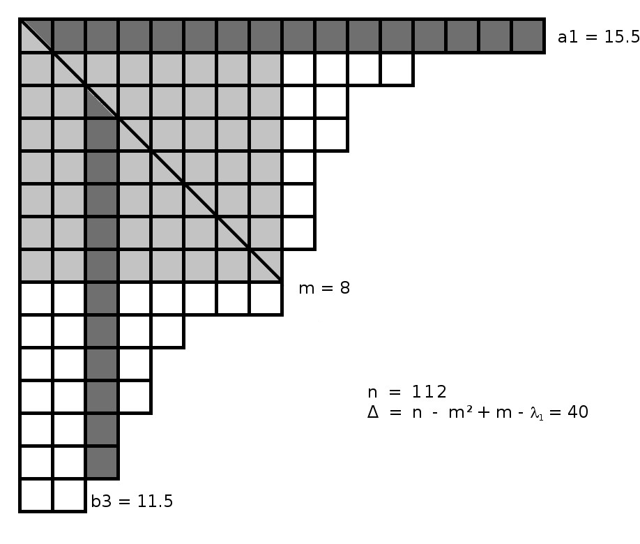
Figure 1. Partition $\lambda$ in Frobenius notation.

We now state our asymptotic evaluation of the character ratio.

Theorem 5.

Let $n$ be large, let $2\leq k\leq n$, and let $C$ be the class of $k$ cycles on $S_{n}$. Let $\lambda\vdash n$ be a partition of $n$ with Frobenius notation $\lambda=(a_{1},...,a_{m}|b_{1},...,b_{m})$.

1. (Long first row) Let $0<\epsilon<\frac{1}{2}$, let $r=n-\lambda_{1}$ and suppose that $r+k+1<(\frac{1}{2}-\epsilon)n$. Then

   (9) $$\frac{\chi^{\lambda}(C)}{f^{\lambda}} =\frac{(a_{1}-\frac{1}{2})^{\underline{k}}}{n^{\underline{k}}}\prod_{j=2}^{m}\frac{a_{1}-a_{j}-k}{a_{1}-a_{j}}\prod_{j=1}^{m}\frac{a_{1}+b_{j}}{a_{1}+b_{j}-k}$$

   $$+O_{\epsilon}\left(\exp\left(k\left[\log\frac{(1+\epsilon)(k+1+r)}{n-k}+O_{\epsilon}\left(r^{-\frac{1}{2}}\right)\right]\right)\right).$$

   If $r<k$ then the error term is actually 0.

2. (Large $k$, short first row and column) Let $\theta>\frac{2}{3}$. There exists $\epsilon(\theta)>0$ such that, for all $n$ sufficiently large, for all $k$ with $6\log n\leq k\leq\epsilon n$ and for all $\lambda\vdash n$ such that $b_{1}\leq a_{1}\leq e^{-\theta}n$,

   $$\left|\frac{\chi^{\lambda}(C)}{f^{\lambda}}\right|\leq e^{\frac{-k}{2}}.$$

3. (Asymptotic expansion) Let $0<\epsilon<\frac{1}{2}$ and suppose now that $k<n^{\frac{1}{2}-\epsilon}$. We have the approximate formula

   (10) $$\frac{\chi^{\lambda}(C)}{f^{\lambda}}= \sum_{a_{i}>kn^{\frac{1}{2}}}\frac{a_{i}^{k}}{n^{k}}\left(1+O_{\epsilon}\left(\frac{kn^{\frac{3}{4}+\epsilon}}{a_{i}}\right)\right)$$

   $$\;\;+(-1)^{k-1}\sum_{b_{i}>kn^{\frac{1}{2}}}\frac{b_{i}^{k}}{n^{k}}\left(1+O_{\epsilon}\left(\frac{kn^{\frac{3}{4}+\epsilon}}{b_{i}}\right)\right)$$

   $$\;\;+O_{\epsilon}\left(n^{\frac{1}{2}}(\log n)^{2}\left(\frac{k\log^{2}n}{\sqrt{n}}\right)^{k}\right).$$

This Theorem is the main technical result of the paper. Actually it gives more than we will need, and we apply the detailed statement of part c. only in the case when the cycle length $k$ is relatively short, $k\leq 6\log n$. The cruder bounds of parts a. and b. suffice when the cycle length $k$ is larger.

4. Proof of Theorem 5

When $C$ is the class of $k$ cycles Frobenius [6] (see [7], p.52 ex. 4.17 b) proved a famous formula that expresses the character ratio of a given representation at $C$ as the ‘residue at $\infty$’ of a meromorphic function depending upon the representation. In Frobenius notation, and using the falling power

$$z^{\underline{r}}=z(z-1)...(z-r+1),$$

the formula is

(11) $$\frac{\chi^{\lambda}(C)}{f^{\lambda}} =\frac{-1}{kn^{\underline{k}}}\frac{1}{2\pi i}\oint F_{k}^{a,b}(z)dz,\quad F_{k}^{a,b}(z)=\left(z+\frac{k-1}{2}\right)^{\underline{k}}F^{a}_{k}(z)F^{b}_{k}(z)$$

$$F^{a}_{k}(z)=\prod_{j=1}^{m}\frac{z-a_{j}-\frac{k}{2}}{z-a_{j}+\frac{k}{2}},\quad F^{b}_{k}(z)=\prod_{j=1}^{m}\frac{z+b_{j}+\frac{k}{2}}{z+b_{j}-\frac{k}{2}}$$

where the integration has winding number 1 around each (finite) pole of the integrand. [Note that our $(a_{i},b_{i})$ correspond to $(b_{m-i+1}+\frac{1}{2},a_{m-i+1}+\frac{1}{2})$ of [7], and replace $y$ there with our $z=y-\frac{k-1}{2}$.]

Our proof of Theorem 5 is an asymptotic estimation of this integral. We first record several properties of $F_{k}^{a,b}$ in the following lemma.

Lemma 6.

Let $\lambda=(a_{1},...,a_{m}|b_{1},...,b_{m})$ be a partition of $n$ in Frobenius notation.

1. Each of $F_{k}^{a}(z)$ and $F_{k}^{b}(z)$ has at most $\sqrt{n}$ poles.

2. If $k>n$ then $F_{k}^{a,b}(z)$ is holomorphic.

Denote by $\lambda^{\prime}=\lambda\setminus\lambda_{1}=(a_{1}^{\prime},...,a_{m^{\prime}}^{\prime}|b_{1}^{\prime},...,b_{m^{\prime}}^{\prime})$ the partition of $n-\lambda_{1}$ found by deleting the first row of $\lambda$.

1. We have

   $$F_{k}^{a,b}(z)\frac{z-a_{1}+\frac{k}{2}}{z-a_{1}-\frac{k}{2}}=F_{k}^{a^{\prime},b^{\prime}}(z+1).$$

2. If $a_{1}>n-k-\frac{1}{2}$ and if $n\geq 2k$ then $F_{k}^{a,b}(z)$ has a single simple pole at $z=a_{1}-\frac{k}{2}$.

Proof.

The first item follows from the bound for the diagonal $m\leq\sqrt{n}$, since both $F_{k}^{a}$ and $F_{k}^{b}$ are products of $m$ terms.

For 2., first observe that $a_{i}$ and $b_{i}$ are strictly decreasing so that the poles of $F_{k}^{a}(z)$ are all simple, as are the poles of $F_{k}^{b}(z)$. Since $k>n$, $a_{i}+b_{j}-k<0$, so $a_{i}-\frac{k}{2}\neq\frac{k}{2}-b_{j}$. Thus the poles of $F_{k}^{a}(z)F_{k}^{b}(z)$ are all simple, and are all cancelled by the factor of $\left(z+\frac{k-1}{2}\right)^{\underline{k}}$.

For 3., observe that deleting the first row of the diagram for $\lambda$ shifts the diagonal down one square. Thus, if $b_{m}=\frac{1}{2}$ then $m^{\prime}=m-1$ and

$$\forall\;1\leq i\leq m^{\prime},\quad a_{i}^{\prime}=a_{i+1}+1,\quad b_{i}^{\prime}=b_{i}-1.$$

In this case, accounting for the lost factor from $b_{m}$,

(12) $$F^{a}_{k}(z)F^{b}_{k}(z)\cdot\frac{z-a_{1}+\frac{k}{2}}{z-a_{1}-\frac{k}{2}}=F^{a^{\prime}}_{k}(z+1)F^{b^{\prime}}_{k}(z+1)\frac{z+\frac{k+1}{2}}{z-\frac{k-1}{2}}.$$

If instead $b_{m}>\frac{1}{2}$ then $a_{m}=\frac{1}{2}$, which implies $m^{\prime}=m$, and

$$\forall\;1\leq i\leq m-1,\quad a_{i}^{\prime}=a_{i+1}+1,\;a_{m}^{\prime}=\frac{1}{2},\quad\forall\;1\leq j\leq m,\quad b_{j}^{\prime}=b_{j}-1.$$

Thus (12) still holds, the new factor accounting for the introduction of $a_{m}^{\prime}=\frac{1}{2}$. Thus, in either case,

$$F_{k}^{a,b}(z) \cdot\frac{z-a_{1}+\frac{k}{2}}{z-a_{1}-\frac{k}{2}}=\left(z+\frac{k-1}{2}\right)^{\underline{k}}F^{a^{\prime}}_{k}(z+1)F^{b^{\prime}}_{k}(z+1)\frac{z+\frac{k+1}{2}}{z-\frac{k-1}{2}}$$

$$=\left(z+\frac{k+1}{2}\right)^{\underline{k}}F^{a^{\prime}}_{k}(z+1)F^{b^{\prime}}_{k}(z+1)$$

$$=F_{k}^{a^{\prime},b^{\prime}}(z+1).$$

For 4., the condition $a_{1}>n-k-\frac{1}{2}$ and $n\geq 2k$ implies that $a_{1}>k-\frac{1}{2}$. Thus, for all $i$, $a_{1}+b_{i}>k$, so that $a_{1}-\frac{k}{2}\neq\frac{k}{2}-b_{i}$, and $a_{1}-\frac{k}{2}$ is a simple pole of $F_{k}^{a}(z)F_{k}^{b}(z)$. Furthermore, it is not cancelled by $\left(z+\frac{k-1}{2}\right)^{\underline{k}}$, so that $a_{1}-\frac{k}{2}$ is a simple pole of $F_{k}^{a,b}(z)$. It is the only pole, since $F_{k}^{a^{\prime},b^{\prime}}(z)$ has $n-\lambda_{1}<k$, hence is holomorphic. ∎

Parts a. and b. of Theorem 5 are more easily proven. We give these proofs immediately, and then prove several lemmas before proving part c.

Proof of Theorem 5 part a..

In this part, the first row $\lambda_{1}$ of partition $\lambda$ is significantly larger than the remainder of the partition, of size $r$. We extract a residue contribution from the pole corresponding to $\lambda_{1}$, and bound the remainder of the character ratio by approximating it with a character ratio on $S_{r}$.

Observe that $\sum_{i>1}a_{i}+\sum_{i}b_{i}=n-a_{1}=r+\frac{1}{2}$. Recall that we assume $r+k+1\leq\left(\frac{1}{2}-\epsilon\right)n$, and that this part of the theorem is the asymptotic

$$\frac{\chi^{\lambda}(C)}{f^{\lambda}} =\frac{(a_{1}-\frac{1}{2})^{\underline{k}}}{n^{\underline{k}}}\prod_{j=2}^{m}\frac{a_{1}-a_{j}-k}{a_{1}-a_{j}}\prod_{j=1}^{m}\frac{a_{1}+b_{j}}{a_{1}+b_{j}-k}$$

$$+O_{\epsilon}\left(\exp\left(k\left[\log\frac{(1+\epsilon)(k+1+r)}{n-k}+O_{\epsilon}\left(r^{-\frac{1}{2}}\right)\right]\right)\right),$$

with the error equal to 0 if $r<k$.

The poles of $F_{k}^{a,b}$ are among the points $a_{i}-\frac{k}{2}$, $\frac{k}{2}-b_{i}$, $i=1,...,k$, some of which may be cancelled by the numerator. The condition $k+1+r\leq\left(\frac{1}{2}-\epsilon\right)n$ guarantees that

$$a_{1}-\frac{k}{2}=n-r-\frac{k+1}{2}>\left(\frac{1}{2}+\epsilon\right)n.$$

Since $a_{i},b_{j}\leq r+\frac{1}{2}$ for $i\geq 2$, $j\geq 1$, it follows that $a_{1}-\frac{k}{2}$ is the furthest pole from zero of the function $F^{a}_{k}(z)F^{b}_{k}(z)$, and that this is a simple pole of $F_{k}^{a,b}(z)$.

Set $R=(1+\epsilon)\left(r+\frac{k+1}{2}\right)$ and notice

$$R<\frac{n}{2}<a_{1}-\frac{k}{2},\qquad R>\max_{i\geq 2,j\geq 1}\left(\left|a_{i}-\frac{k}{2}\right|,\left|b_{j}-\frac{k}{2}\right|\right),$$

so that $a_{1}-\frac{k}{2}$ is outside the loop $|z|=R$, while all other poles are inside. Thus

(13) $$\frac{\chi^{\lambda}(C)}{f^{\lambda}}=\frac{-1}{kn^{\underline{k}}}\mathrm{Res}_{z=a_{1}-\frac{k}{2}}F_{k}^{a,b}(z)+\frac{-1}{kn^{\underline{k}}}\frac{1}{2\pi i}\int_{|z|=R}F_{k}^{a,b}(z)dz.$$

The residue term is equal to the main term of the theorem, so it remains to bound the integral.

Recall the notation $(a_{1}^{\prime},...,a_{m^{\prime}}^{\prime}|b_{1}^{\prime},...,b_{m^{\prime}}^{\prime})=\lambda\setminus\lambda_{1}$, and that

$$F_{k}^{a,b}(z)=\frac{z-a_{1}-\frac{k}{2}}{z-a_{1}+\frac{k}{2}}F_{k}^{a^{\prime},b^{\prime}}(z+1).$$

Thus we express the integral of (13) as

(14) $$\frac{-1}{kn^{\underline{k}}}\frac{1}{2\pi i}\int_{|z|=R}F_{k}^{a,b}(z)dz=\frac{-1}{kn^{\underline{k}}}\frac{1}{2\pi i}\int_{|z|=R}F_{k}^{a^{\prime},b^{\prime}}(z+1)\frac{z-a_{1}-\frac{k}{2}}{z-a_{1}+\frac{k}{2}}dz.$$

When $k>r$, $F_{k}^{a^{\prime},b^{\prime}}(z+1)$ is holomorphic, and so (14) is zero, which proves the latter claim of the theorem. Thus we may now assume that $r\geq k$.

On the contour $|z|=R$,

$$\left|z-a_{1}+\frac{k}{2}\right|\geq a_{1}-R-\frac{k}{2}\geq n-(2+\epsilon)\left(r+\frac{k+1}{2}\right)\gg_{\epsilon}n,$$

so that $\left|\frac{z-a_{1}-\frac{k}{2}}{z-a_{1}+\frac{k}{2}}-1\right|=O_{\epsilon}\left(\frac{k}{n}\right).$ Thus (14) is equal to ($C^{\prime}$ is the $k$ cycle class on $S_{r}$)

(15) $$\frac{r^{\underline{k}}}{n^{\underline{k}}}\frac{\chi^{\lambda\setminus\lambda_{1}}(C^{\prime})}{f^{\lambda\setminus\lambda_{1}}}+O_{\epsilon}\left(\frac{k}{n}\frac{1}{kn^{\underline{k}}}\int_{|z|=R}\left|F_{k}^{a^{\prime},b^{\prime}}(z+1)\right|d|z|\right).$$

We bound the first term by $\frac{r^{\underline{k}}}{n^{\underline{k}}}$, since all character ratios are bounded by 1.

To bound the integral, note that $F^{a^{\prime}}_{k}(z)$ and $F^{b^{\prime}}_{k}(z)$ each have at most $\sqrt{r}$ poles. On the contour $|z|=R$,

$$\left|\frac{z-a_{i}-\frac{k}{2}}{z-a_{i}+\frac{k}{2}}\right|\leq 1+O_{\epsilon}\left(\frac{k}{r}\right),$$

and the terms in $F^{b^{\prime}}_{k}(z)$ are bounded similarly. It follows that on $|z|=R$,

$$|F^{a^{\prime}}_{k}(z+1)F^{b^{\prime}}_{k}(z+1)|\leq\exp\left(O_{\epsilon}\left(\frac{k}{\sqrt{r}}\right)\right).$$

Meanwhile, also on $|z|=R$,

$$\left|\left(z+\frac{k+1}{2}\right)^{\underline{k}}\right|\leq\left(|z|+\frac{k+1}{2}\right)^{k}\leq\left((1+\epsilon)(k+1+r)\right)^{k}.$$

Putting these bounds together, we deduce a bound for the second term of (15) of

$$\frac{1}{n\cdot n^{\underline{k}}} \frac{1}{2\pi}\int_{|z|=R}|F^{a^{\prime},b^{\prime}}_{k}(z+1)|d|z|\leq\frac{1}{n^{\underline{k}}}\sup_{|z|=R}\left|F_{k}^{a^{\prime},b^{\prime}}(z+1)\right|$$

$$=O_{\epsilon}\left(\frac{1}{n^{\underline{k}}}\exp\left(k\left[\log\left((1+\epsilon)(r+k+1)\right)+O_{\epsilon}\left(\frac{1}{\sqrt{r}}\right)\right]\right)\right).$$

To complete the proof of the theorem, use $n^{\underline{k}}\geq(n-k)^{k}$ and note that the term $\frac{r^{\underline{k}}}{n^{\underline{k}}}$ from the character ratio in (15) is trivially absorbed into this error term. ∎

Proof of Theorem 5 part b..

Choose $\theta_{1}$ with $\frac{2}{3}<\theta_{1}<\theta$. Since the poles of $F^{a,b}_{k}$ are among $a_{i}-\frac{k}{2}$ and $\frac{k}{2}-b_{i}$, $i=1,2,3,...$, choosing $\epsilon=\epsilon(\theta)>0$ sufficiently small, $a_{i},b_{i}<e^{-\theta}n$ and $k\leq\epsilon n$ guarantees that the contour $|z|=R=e^{-\theta_{1}}n$ contains all poles of $F^{a,b}_{k}(z)$. Thus

$$\frac{\chi^{\lambda}(C)}{f^{\lambda}}=\frac{-1}{kn^{\underline{k}}}\frac{1}{2\pi i}\int_{|z|=R}F^{a,b}_{k}(z)dz.$$

Write $\frac{1}{kn^{\underline{k}}}F^{a,b}_{k}(z)=\frac{(z+\frac{k-1}{2})^{\underline{k}}}{kn^{\underline{k}}}F^{a}_{k}(z)F^{b}_{k}(z)$. Since $k\leq\epsilon n$, for $|z|=R$,

$$\left|\frac{(z+\frac{k-1}{2})^{\underline{k}}}{n^{\underline{k}}}\right|\leq\frac{\left(R+\frac{k}{2}\right)^{k}}{(n-k)^{k}}\leq\exp(k(-\theta_{1}+o(1))),$$

with $o(1)$ indicating a quantity that may be made arbitrarily small with a sufficiently small choice of $\epsilon$. Also, $F^{a}_{k}(z)$ and $F^{b}_{k}(z)$ are each composed of at most $\sqrt{n}$ factors, each of size at most $1+O_{\theta,\theta_{1},\epsilon}(\frac{k}{n})$. We deduce that for $|z|=R$,

$$\left|\frac{1}{kn^{\underline{k}}}F^{a,b}_{k}(z)\right|\leq\exp\left(k\left(-\theta_{1}+o_{\theta,\theta_{1}}(1)\right)\right),$$

the error term requiring that first $\epsilon$ be small, and then that $n$ be large. The length of the contour is $O(n)=O\left(\exp\left(\frac{k}{6}\right)\right)$. Since $\theta_{1}>\frac{1}{2}+\frac{1}{6}$, it follows that the bound $\exp\left(-\frac{k}{2}\right)$ holds for the character ratio for all $n$ sufficiently large. ∎

We now turn to part c. of Theorem 5. We will again estimate the integral

(16) $$\frac{\chi^{\lambda}(C)}{f^{\lambda}}=\frac{-1}{kn^{\underline{k}}}\frac{1}{2\pi i}\oint F_{k}^{a,b}(z)dz,$$

but the idea now will be to evaluate clumps of poles together. With an appropriate choice of contour, at any given point the poles that are sufficiently far away make an essentially constant contribution to the integrand, and so may be safely removed, simplifying the integral.

Denote by

$$\mathcal{P}=\left\{a_{j}-\frac{k}{2}:1\leq j\leq m\right\}\cup\left\{\frac{k}{2}-b_{j}:1\leq j\leq m\right\}$$

the multi-set (that is, set counted with multiplicities) of poles of $F_{k}^{a}(z)$ and $F_{k}^{b}(z)$. One trivial fact concerning the distribution of poles in $\mathcal{P}$ is the following bound.

Lemma 7.

For any $x>0$,

$$\#\{p\in\mathcal{P}:|p|>x\}\leq\frac{n+km}{x}.$$

Indeed, this follows from the fact that

$$\sum_{i=1}^{m}\left|a_{i}-\frac{k}{2}\right|+\sum_{i=1}^{m}\left|\frac{k}{2}-b_{i}\right|\leq km+\sum a_{i}+\sum b_{i}=km+n.$$

A useful consequence is that for $x$ real, $|x|>k\sqrt{n}$, we can always find a real point $y$ nearby $x$ with large distance from all poles in $\mathcal{P}$.

Definition 1.

Let $x\in\mathbb{R}\setminus 0$ and let $L>0$ be a parameter. We say that a real number $y$ is $L$-well-spaced for $x$ with respect to $\mathcal{P}$ if the bound is satisfied

(17) $$\sum_{p\in\mathcal{P}:|p-x|<\frac{|x|}{2}}\frac{1}{|p-y|}\leq\frac{L}{|x|}.$$

The following lemma says that if $|x|$ is sufficiently large, then there are always many points $y$ nearby $x$ that are well-spaced for $x$ with respect to $\mathcal{P}$.

Lemma 8.

Let $n>e^{5}$ and let $1<k<\sqrt{n}$. Let $x$ be real with $|x|>k\sqrt{n}\log n$. Then there exists a real $y$ with $|y-x|<\sqrt{n}$ which is $4\sqrt{n}\log n$-well-spaced for $x$ with respect to $\mathcal{P}$.

Proof.

Let $I$ be the interval $I=\{y:|y-x|<\sqrt{n}\}$. By Lemma 7, the interval $I$ contains at most

$$\frac{n+km}{|x|-\sqrt{n}}\leq\frac{2n}{|x|-\sqrt{n}}\leq\frac{2.5\sqrt{n}}{k\log n}$$

poles of $\mathcal{P}$. Deleting the segment of radius $k$ around each pole in $\mathcal{P}\cap I$ removes a set of total length at most

$$\frac{5\sqrt{n}}{\log n}\leq\sqrt{n}$$

leaving $I^{\prime}$ with $|I^{\prime}|\geq\frac{|I|}{2}=\sqrt{n}$. Now

$$\frac{1}{|I^{\prime}|}\int_{y\in I^{\prime}}\sum_{p\in\mathcal{P},|p-x|<\frac{|x|}{2}}\frac{dy}{|y-p|} \leq\frac{1}{|I^{\prime}|}\sum_{p\in\mathcal{P},|p-x|<\frac{|x|}{2}}\int_{u\in I,|u-p|\geq k}\frac{du}{|u-p|}$$

$$\leq\frac{1}{|I^{\prime}|}\sum_{p\in\mathcal{P},|p-x|<\frac{|x|}{2}}2\times\int_{k}^{\sqrt{n}}\frac{du}{u}$$

(18) $$\leq\frac{\log n}{|I^{\prime}|}\left|\left\{p\in\mathcal{P}:|p-x|<\frac{|x|}{2}\right\}\right|.$$

Applying the cardinality bound of Lemma 7 a second time (recall $|I^{\prime}|\geq\sqrt{n}$) we obtain a bound for (18) of

$$\frac{\log n}{\sqrt{n}}\frac{(n+km)}{\frac{|x|}{2}}\leq\frac{4\sqrt{n}\log n}{|x|}.$$

It follows that a typical point $y\in I^{\prime}$ is $4\sqrt{n}\log n$-well-spaced for $x$. ∎

Recall that $k\leq n^{\frac{1}{2}-\epsilon}$. We now assume, as we may, that $n$ is sufficiently large to guarantee $k\leq\frac{\sqrt{n}}{(\log n)^{2}}$ and we choose a sequence of well-spaced points at which we partition our integral.

To find our sequence of points, first set

$$x_{0}=\frac{k}{2}\sqrt{n}(\log n)^{2}$$

and

$$x_{j}=x_{0}+2j\sqrt{n},\qquad j=1,2,...$$

for those $j$ such that $x_{j}\leq n+4\sqrt{n}$. In each interval

$$[x_{j}-\sqrt{n},x_{j}+\sqrt{n}),\qquad j=0,1,2,...$$

apply Lemma 8 to find $y_{j}^{+}$, a $4\sqrt{n}\log n$-well-spaced point for $x_{j}$. Also find a point $y_{j}^{-}$ in each interval $(-x_{j}-\sqrt{n},-x_{j}+\sqrt{n}]$ which is $4\sqrt{n}\log n$-well-spaced for $-x_{j}$. Thus we have the disjoint intervals

$$I_{0}=(y_{0}^{-},y_{0}^{+}),\qquad I_{j}^{+}=[y_{j-1}^{+},y_{j}^{+}),\quad I_{j}^{-}=(y_{j}^{-},y_{j-1}^{-}],\quad j=1,2,3,...$$

which together cover

$$(-n-\sqrt{n},n+\sqrt{n}).$$

Let $q_{j}^{+}$ (resp. $q_{j}^{-},q_{0}$) be the number of poles of $\mathcal{P}$ contained in $I_{j}^{+}$, (resp. $I_{j}^{-},I_{0}$).

Around each interval $I_{j}^{+},$ $j\geq 1$ we draw a rectangular box

$${\mathcal{B}}_{j}^{+}=\left\{z\in\mathbb{C}:y_{j-1}^{+}\leq\Re(z)\leq y_{j}^{+},\;|\Im(z)|\leq kq_{j}^{+}\right\}$$

and similarly around $I_{j}^{-}$. If $q_{j}^{\pm}=0$ then the box may be discarded. We also draw a large box ${\mathcal{B}}_{0}$ containing the origin, with endpoints at $y_{0}^{-}\pm ik\sqrt{n},y_{0}^{+}\pm ik\sqrt{n}$. A permissible contour with which to apply integral formula (16) is given by

$$\partial{\mathcal{B}}_{0}\cup\bigcup_{j\geq 1}\partial{\mathcal{B}}_{j}^{+}\cup\bigcup_{j\geq 1}\partial{\mathcal{B}}_{j}^{-},$$

each box being positively oriented, see figure 2. We use a somewhat shortened version of this contour.

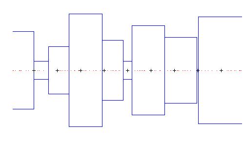
Figure 2. Schematic of the boxes ${\mathcal{B}}_{j}$. Between successive equally spaced points $x_{j},x_{j+1}$ denoted by (+), point $y_{j}$ is chosen to be well-spaced from the set of poles (red). Box ${\mathcal{B}}_{j}$ has vertical edges at $\Re(z)=y_{j-1},y_{j}$, and height proportional to the number of poles contained.

In what follows we treat only the integrals around the boxes ${\mathcal{B}}_{j}^{+}$ and ${\mathcal{B}}_{0}$, and we drop superscripts (so we write e.g. $q_{j}$ for $q_{j}^{+}$, $I_{j}$ for $I_{j}^{+}$ etc). The argument may be carried out symmetrically for ${\mathcal{B}}_{j}^{-}$. The main proposition is as follows.

Proposition 9.

Let $j\geq 1$. There exists a piecewise linear contour $\mathcal{C}_{j}$, having total length

$$|\mathcal{C}_{j}|\leq 12kq_{j}n^{\frac{1}{4}},$$

such that $\mathcal{C}_{j}$ has winding number 1 around each pole $p\in\mathcal{P}\cap{\mathcal{B}}_{j}$ and winding number 0 around all poles $p^{\prime}\in\mathcal{P}\setminus{\mathcal{B}}_{j}$. For $z\in\mathcal{C}_{j}$, $F_{k}^{a,b}(z)$ satisfies

(19) $$F^{a,b}_{k}(z)=\left(x_{j}+\frac{k-1}{2}\right)^{\underline{k}}\prod_{p\in\mathcal{P}\cap{\mathcal{B}}_{j}}\frac{z-p-k}{z-p}+O\left(kx_{j}^{k-1}\sqrt{n}\log n\right).$$

Proof.

Recall that ${\mathcal{B}}_{j}$ is a box containing $q_{j}$ poles and surrounding interval $I_{j}=[y_{j-1},y_{j})$, with corners at

$$y_{j-1}\pm ikq_{j},\qquad y_{j}\pm ikq_{j}.$$

Recall also that $y_{j}\in[x_{j}-\sqrt{n},x_{j}+\sqrt{n})$ and $x_{j}-x_{j-1}=2\sqrt{n}$, so that $|y_{j}-y_{j-1}|\leq 4\sqrt{n}$.

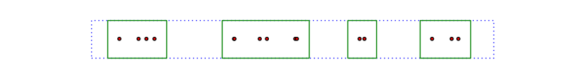
Figure 3. Schematic of contour ${\mathcal{C}}_{j}$. Poles in red, box ${\mathcal{B}}_{j}$ in blue, ${\mathcal{C}}_{j}$ in green.

To form $\mathcal{C}_{j}$ we shorten the contour $\partial{\mathcal{B}}_{j}$. At each pole $p\in{\mathcal{B}}_{j}$ consider the segment

$$S_{p}=[p-kq_{j},p+kq_{j}].$$

If there exists a subinterval $J$ of interval $I_{j}$ that is not covered by $\cup_{p\in\mathcal{P}\cap{\mathcal{B}}_{j}}S_{p}$ then such $J$ may be discarded from the box ${\mathcal{B}}_{j}$ by drawing vertical segments at the endpoints of $J$ and deleting the parts of ${\mathcal{B}}_{j}$ vertically above and below $J$. Deleting subintervals in this way if it reduces the total perimeter, or allowing them to remain when the perimeter is increased, we arrive at a contour $\mathcal{C}_{j}$ which is the union of some rectangles, and has total length at most

$$|\mathcal{C}_{j}|\leq\min(8\sqrt{n}+4kq_{j},8kq_{j}^{2}),$$

the first term bounding the result of doing nothing, and the second bounding the length of a contour with an individual box around every pole. Using $\min(a,b)\leq\sqrt{ab}$, we have the bound

$$|\mathcal{C}_{j}|\leq 4kq_{j}+\min(8\sqrt{n},8kq_{j}^{2})\leq 4kq_{j}+8kq_{j}n^{\frac{1}{4}}\leq 12kq_{j}n^{\frac{1}{4}}.$$

We now prove the formula (19). Observe that by Lemma 7, the number of poles $q_{j}$ in $\mathcal{P}\cap{\mathcal{B}}_{j}$ satisfies $q_{j}\ll\frac{n}{x_{j}}\ll\frac{\sqrt{n}}{k}$, so that each point of $\mathcal{C}_{j}$ has distance $O(\sqrt{n})$ from $x_{j}$. Thus

$$\forall z\in\mathcal{C}_{j},\qquad\left(z+\frac{k-1}{2}\right)^{\underline{k}}=\left(x_{j}+\frac{k-1}{2}\right)^{\underline{k}}\left(1+O\left(\frac{k\sqrt{n}}{x_{j}}\right)\right).$$

In particular, it follows that

(20) $$\forall z\in\mathcal{C}_{j},\qquad F_{k}^{a,b}(z)=\left(1+O\left(\frac{k\sqrt{n}}{x_{j}}\right)\right)\left(x_{j}+\frac{k-1}{2}\right)^{\underline{k}}F_{k}^{a}(z)F_{k}^{b}(z).$$

We prove

(21) $$\forall z\in\mathcal{C}_{j},\qquad F_{k}^{a}(z)F_{k}^{b}(z)=\left(1+O\left(\frac{k\sqrt{n}\log n}{x_{j}}\right)\right)\cdot\prod_{p\in\mathcal{P}\cap{\mathcal{B}}_{j}}\frac{z-p-k}{z-p},$$

and

(22) $$\forall z\in\mathcal{C}_{j},\qquad\prod_{p\in\mathcal{P}\cap{\mathcal{B}}_{j}}\frac{z-p-k}{z-p}=O(1).$$

Inserted in (20) these combine to prove the formula (19), (use $\left(x_{j}+\frac{k-1}{2}\right)^{\underline{k}}\leq x_{j}^{k}$).

We first consider (21). This estimate is equivalent to

$$\forall z\in\mathcal{C}_{j},\qquad\prod_{p\in\mathcal{P}\setminus{\mathcal{B}}_{j}}\frac{z-p\mp k}{z-p}=1+O\left(\frac{k\sqrt{n}\log n}{x_{j}}\right),$$

the sign determined according as $p$ is a pole from $F_{k}^{a}$ or $F_{k}^{b}$. Say a pole $p\in\mathcal{P}\setminus{\mathcal{B}}_{j}$ is ‘good’ if $|p-x_{j}|>\frac{x_{j}}{2}$ and ‘bad’ otherwise. For $z\in\mathcal{C}_{j}$,

$$|z-x_{j}|=O(\sqrt{n})<\frac{x_{j}}{3}$$

if $n$ is sufficiently large, which implies that for good $p$, $|z-p|\geq\frac{x_{j}}{6}$. Since the total number of poles is $O(\sqrt{n})$, the product over good poles evidently satisfies the bound

$$\prod_{p\text{ good}}\left(1\mp\frac{k}{z-p}\right)=1+O\left(\frac{k\sqrt{n}}{x_{j}}\right).$$

Since it is not contained in the box ${\mathcal{B}}_{j}$, a bad pole $p$ necessarily lives in the complement $\mathbb{R}\setminus[y_{j-1},y_{j}]$, and either satisfies $p>y_{j}$ and $|p-x_{j}|\leq\frac{x_{j}}{2}$ or else $p<y_{j-1}$, which entails $\frac{x_{j}}{2}\leq p\leq x_{j}$. Since $\frac{x_{j-1}}{2}<\frac{x_{j}}{2}$, and $\frac{3x_{j-1}}{2}>x_{j}$ (at least if $n$ is sufficiently large), it follows that in the second case, $|p-x_{j-1}|\leq\frac{x_{j-1}}{2}$. Thus, for $z\in\mathcal{C}_{j}$, the fact that $y_{j-1}\leq\Re(z)\leq y_{j}$ implies

$$\sum_{p\text{ bad},\;p>y_{j}}\frac{1}{|z-p|}\leq\sum_{\begin{subarray}{c}p>y_{j}\\ |p-x_{j}|<\frac{x_{j}}{2}\end{subarray}}\frac{1}{p-y_{j}}\leq\frac{4\sqrt{n}\log n}{x_{j}}$$

and

$$\sum_{p\text{ bad},\;p<y_{j-1}}\frac{1}{|z-p|}\leq\sum_{\begin{subarray}{c}p<y_{j-1}\\ |p-x_{j-1}|<\frac{x_{j-1}}{2}\end{subarray}}\frac{1}{y_{j-1}-p}\leq\frac{4\sqrt{n}\log n}{x_{j-1}}\leq\frac{8\sqrt{n}\log n}{x_{j}},$$

by invoking the $4\sqrt{n}\log n$ well-spaced property of $y_{j-1}$ and $y_{j}$. It follows

$$\prod_{p\text{ bad}}\left(\frac{z-p\mp k}{z-p}\right)=1+O\left(\frac{k\sqrt{n}\log n}{x_{j}}\right),$$

proving (21).

To prove (22) we consider two cases. When either $\Re(z)=y_{j-1}$ or $\Re(z)=y_{j}$, observe that for each $p\in\mathcal{P}\cap{\mathcal{B}}_{j}$,

$$|p-x_{j}|\leq 2\sqrt{n}\leq\frac{x_{j}}{2}.$$

Also, since $x_{j}-x_{j-1}=2\sqrt{n}$,

$$|p-x_{j-1}|\leq 4\sqrt{n}\leq\frac{x_{j-1}}{2}\qquad(n\text{ large}).$$

Thus, invoking the well-spaced property of $y_{j-1}$ and $y_{j}$,

$$\sum_{p\in\mathcal{P}\cap{\mathcal{B}}_{j}}\frac{1}{|p-y_{j-1}|}\leq\frac{4\sqrt{n}\log n}{x_{j-1}},\qquad\sum_{p\in\mathcal{P}\cap{\mathcal{B}}_{j}}\frac{1}{|p-y_{j}|}\leq\frac{4\sqrt{n}\log n}{x_{j}}$$

so that if $\Re(z)=y_{j-1}$,

$$\prod_{p\in\mathcal{P}\cap{\mathcal{B}}_{j}}\left(1-\frac{k}{z-p}\right)\leq\exp\left(O\left(\frac{k\sqrt{n}\log n}{x_{j-1}}\right)\right)=O(1),$$

and similarly when $\Re(z)=y_{j}$.

When $\Re(z)\not\in\{y_{j-1},y_{j}\}$ then $|z-p|\geq kq_{j}$ for each $p\in\mathcal{P}\cap{\mathcal{B}}_{j}$, so that in this case the bound

$$\prod_{p\in\mathcal{P}\cap{\mathcal{B}}_{j}}\left(1-\frac{k}{z-p}\right)=O(1)$$

is immediate from $|\mathcal{P}\cap{\mathcal{B}}_{j}|=q_{j}$. Thus (22) holds in either case.

∎

We now bound integration around the box ${\mathcal{B}}_{0}$.

Lemma 10.

Assume $n>e^{5}$. We have

$$\frac{-1}{kn^{\underline{k}}}\frac{1}{2\pi i}\oint_{\partial{\mathcal{B}}_{0}}F^{a,b}_{k}(z)dz=O\left(\sqrt{n}(\log n)^{2}\left(\frac{k\log^{2}n}{n^{\frac{1}{2}}}\right)^{k}\right).$$

Proof.

Since ${\mathcal{B}}_{0}$ is a box with corners at $y_{0}^{\pm}\pm ik\sqrt{n}$, the integral has length $O(k\sqrt{n}(\log n)^{2})$, so it will suffice to prove

$$\forall z\in\partial{\mathcal{B}}_{0},\qquad\left|\frac{F_{k}^{a,b}(z)}{kn^{\underline{k}}}\right|=O\left(\frac{1}{k}\left(\frac{k\log^{2}n}{n^{\frac{1}{2}}}\right)^{k}\right).$$

Recall that

$$F_{k}^{a,b}(z)=\left(z+\frac{k-1}{2}\right)^{\underline{k}}F_{k}^{a}(z)F_{k}^{b}(z).$$

Recall also that $|y_{0}^{\pm}\mp x_{0}|\leq\sqrt{n}$ and $x_{0}=\frac{k}{2}\sqrt{n}(\log n)^{2}$. Thus, on $\partial{\mathcal{B}}_{0}$ we have $|\Re z|\leq\frac{k}{2}\sqrt{n}(\log n)^{2}+\sqrt{n}$. Hence, using $k<\sqrt{n}$,

$$\left(z+\frac{k-1}{2}\right)^{\underline{k}} \leq\left(|\Re(z)|+|\Im(z)|+\frac{k-1}{2}\right)^{k}$$

$$\leq\left(\frac{k}{2}\sqrt{n}(\log n)^{2}+2\sqrt{n}+k\sqrt{n}\right)^{k}$$

$$\leq(k\sqrt{n}(\log n)^{2})^{k},$$

the last bound requiring $k+2\leq\frac{k}{2}(\log n)^{2}$, which plainly holds for $n>e^{5}$. Since $n^{\underline{k}}\gg n^{k}$ when $k<\sqrt{n}$, we obtain the required bound for $\sup_{z\in\partial{\mathcal{B}}_{0}}\left|\frac{F_{k}^{a,b}(z)}{kn^{\underline{k}}}\right|$ by checking that

$$\sup_{z\in\partial{\mathcal{B}}_{0}}|F_{k}^{a}(z)F_{k}^{b}(z)|=O(1).$$

To do so, for each $p\in\mathcal{P}$ write the corresponding factor of $F^{a}_{k}(z)$ or $F^{b}_{k}(z)$ as

$$\frac{z-p\pm k}{z-p}=1\pm\frac{k}{z-p}.$$

For a given $z\in\partial{\mathcal{B}}_{0}$, say the pole $p\in\mathcal{P}$ is ‘good’ for $z$ if $|z-p|\geq k\sqrt{n}$. Since the total number of poles in $\mathcal{P}$ is $O(\sqrt{n})$, the part of the product in $F^{a}_{k}(z)F^{b}_{k}(z)$ contributed by good poles is bounded by $O(1)$, so we may consider only the bad poles.

Bad poles exist only if $z$ is on one of the two vertical sides of the box, that is $\Re(z)=y_{0}^{\pm}$. Notice that, e.g.

$$|p-y_{0}^{+}|<k\sqrt{n}\qquad\Rightarrow\qquad|p-x_{0}|<(k+1)\sqrt{n}<\frac{k}{4}\sqrt{n}(\log n)^{2}=\frac{x_{0}}{2}$$

(similarly if $p$ is near $y_{0}^{-}$), and so bad poles satisfy $\min(|p+x_{0}|,|p-x_{0}|)<\frac{x_{0}}{2}$.

By the well-spaced property of $y_{0}^{\pm}$, when $\Re(z)=y_{0}^{\pm}$ we have

$$\sum_{p\text{ bad}}\frac{1}{|z-p|} \leq\sum_{p\text{ bad},p>0}\frac{1}{|y_{0}^{+}-p|}+\sum_{p\text{ bad},p<0}\frac{1}{|y_{0}^{-}-p|}$$

$$\leq\frac{8\sqrt{n}\log n}{x_{0}}\leq\frac{16}{k\log n}.$$

It follows that

$$\prod_{p\text{ bad}}\left(1+\frac{1}{|z-p|}\right)=O(1).$$

∎

We now have all of the estimates that we need to complete the proof of Theorem 5. We use the following integral formula.

Lemma 11.

Let $p_{1},p_{2},...,p_{s}\in\mathbb{C}$ be a sequence of poles and let $d$ be an arbitrary complex number. Then

$$I(p_{1},...,p_{s},d)=\frac{1}{2\pi i}\oint\prod_{j=1}^{s}\frac{z-p_{j}+d}{z-p_{j}}=sd$$

where the contour is such that it has winding number one about each pole.

Proof.

The integral is independent of the appropriate contour, so take the contour to be a large loop containing the poles. We may write the integrand as $\prod_{j=1}^{s}\left(1+\frac{d}{z-p_{j}}\right).$ Differentiating the integrand with respect to $p_{j}$ results in a rational function having total degree $-2$. It follows that $\frac{\partial}{\partial p_{j}}I(p_{1},...,p_{s},d)=0$ for each $j$, since the integral can be made made arbitrarily small by taking the contour to be sufficiently large. Taking $p_{j}=0$ for each $j$, we find that the residue at 0 is $sd$. ∎

Proof of Theorem 5 part c..

Write

$$\frac{\chi^{\lambda}(C)}{f^{\lambda}}=\frac{-1}{kn^{\underline{k}}}\frac{1}{2\pi i}\left\{\oint_{\partial{\mathcal{B}}_{0}}+\sum_{j\geq 1}\oint_{\mathcal{C}_{j}^{+}}+\sum_{j\geq 1}\oint_{\mathcal{C}_{j}^{-}}\right\}F_{k}^{a,b}(z)dz.$$

The contribution from $\partial{\mathcal{B}}_{0}$ is bounded in Lemma 10 by

$$\frac{-1}{kn^{\underline{k}}}\frac{1}{2\pi i}\oint_{\partial{\mathcal{B}}_{0}}F^{a,b}_{k}(z)dz=O\left(\sqrt{n}(\log n)^{2}\left(\frac{k\log^{2}n}{n^{\frac{1}{2}}}\right)^{k}\right).$$

which may be absorbed into the error term of the theorem.

For each $j\geq 1$, write the contribution from the $q_{j}^{+}$ poles inside $\mathcal{C}_{j}^{+}$ as

$$\frac{1}{2\pi i}\int_{\mathcal{C}_{j}^{+}}\left[\frac{-(x_{j}+\frac{k-1}{2})^{\underline{k}}}{kn^{\underline{k}}}\prod_{p\in\mathcal{P}\cap{\mathcal{B}}_{j}}\frac{z-p-k}{z-p}+O\left(\left(\frac{x_{j}}{n}\right)^{k-1}\frac{\log n}{\sqrt{n}}\right)\right]dz.$$

For the main term of this integral, Lemma 11 gives the evaluation

$$\frac{1}{2\pi i}\int_{\mathcal{C}_{j}^{+}}\frac{-(x_{j}+\frac{k-1}{2})^{\underline{k}}}{kn^{\underline{k}}} \prod_{p\in\mathcal{P}\cap{\mathcal{B}}_{j}}\frac{z-p-k}{z-p}dz=q_{j}\frac{\left(x_{j}+\frac{k-1}{2}\right)^{\underline{k}}}{n^{\underline{k}}}$$

$$=\sum_{a_{i}:a_{i}-\frac{k}{2}\in{\mathcal{B}}_{j}^{+}}\left(\frac{a_{i}}{n}\right)^{k}\left(1+O\left(\frac{k\sqrt{n}}{a_{i}}\right)\right),$$

the error resulting since each of the $k$ terms of $\left(x+\frac{k-1}{2}\right)^{\underline{k}}$ is equal to $a_{i}+O(\sqrt{n})$ – we use that $a_{i}=\Omega(k\sqrt{n})$ here. Had we considered $\mathcal{C}_{j}^{-}$ rather than $\mathcal{C}_{j}^{+}$ this main term would involve a sum over the $b_{i}$, with an appropriate sign factor.

The integral of the error term over $\mathcal{C}_{j}$ is bounded trivially by using $|\mathcal{C}_{j}|=O(kq_{j}n^{\frac{1}{4}})$, which gives

$$O\left(kq_{j}n^{\frac{1}{4}}\cdot\left(\frac{x_{j}}{n}\right)^{k-1}\frac{\log n}{\sqrt{n}}\right).$$

The ratio of the error from $\mathcal{C}_{j}$ to the corresponding main term is

$$O\left(\frac{kn^{\frac{3}{4}}\log n}{x_{j}}\right),$$

and since each $a_{i}$ in the sum above is within constants of $x_{j}$, this proves the Theorem.

Note that in the claimed formula of the Theorem, the sums over $a_{i}$ and $b_{j}$ contain terms for which $k\sqrt{n}<a_{i}\leq y_{0}^{+}+\frac{k}{2}$ and $k\sqrt{n}<b_{j}\leq-y_{0}^{-}+\frac{k}{2}$, which do not appear in our evaluation. However, only a bound, rather than an asymptotic, is claimed in this range, so that the theorem is valid with the extra terms discarded. ∎

5. Proof of upper bound for Theorem 2

We now prove the upper bound on mixing time from Theorem 2 by proving Proposition 3. Recall that this proposition is a bound for character ratios at class $C$ of $k$ cycles,

(23) $$\left|\frac{\chi^{\lambda}(C)}{f^{\lambda}}\right|^{\frac{n}{k}(\log n+c)}\leq\frac{1}{f^{\lambda}},$$

uniformly for $k$ less than a fixed constant times $n$ and for all $\lambda\vdash n$.

Before proving the estimate, we collect together several observations. First note that the character ratio bound is trivial for the one-dimensional representations $\lambda=(n),(1^{n})$. Also, exchanging $\lambda$ with its dual $\lambda^{\prime}$ leaves the dimension $f^{\lambda}$ unchanged, and at most changes the sign of $\chi^{\lambda}(C)$, so we will assume without loss of generality that $\lambda$ has $a_{1}\geq b_{1}$. We set $r=n-\lambda_{1}=n-a_{1}-\frac{1}{2}$.

Lemma 12 (Criterion lemma).

To prove the character ratio bound (23), it suffices to prove that for all $n$ larger than the maximum of $k$ and a fixed constant, and for a sufficiently large $c>0$, that for all non-trivial $\lambda$ with $a_{1}\geq b_{1}$,

$$\log\left|\frac{\chi^{\lambda}(C)}{f^{\lambda}}\right|\leq\max\left(\frac{-kr}{n}+\frac{kr\log r}{2n\log n}+\frac{ckr}{n\log n},\frac{-k}{2}+\frac{ck}{\log n}\right).$$

Proof.

By the bound (6) for the dimension, we have (use $\log r!\geq r\log\frac{r}{e}$)

$$f^{\lambda}\leq\binom{n}{r}\sqrt{r!}\leq\frac{n^{r}}{\sqrt{r!}}\leq\exp\left(r\log n-\frac{1}{2}\left(r\log\frac{r}{e}\right)\right)$$

so that a bound of

$$\log\left|\frac{\chi^{\lambda}(C)}{f^{\lambda}}\right|\leq\frac{-kr}{n}+\frac{kr\log r}{2n\log n}+\frac{ckr}{n\log n}$$

is sufficient.

On the other hand, for all $\lambda$, $f^{\lambda}\leq\sqrt{n!}$, so that a bound of

$$\log\left|\frac{\chi^{\lambda}(C)}{f^{\lambda}}\right|\leq\frac{-k}{2}+\frac{ck}{\log n}$$

also suffices. ∎

Our proof splits into two cases depending upon whether $k\geq 6\log n$. The essential tool in both cases will be the evaluation of the character ratio from Theorem 5. For large $k$ we will use only parts a. and b. of that theorem. Recall that part a. had a main term equal to

$$\operatorname{MT}:=\frac{(a_{1}-\frac{1}{2})^{\underline{k}}}{n^{\underline{k}}}\prod_{j=2}^{m}\frac{a_{1}-a_{j}-k}{a_{1}-a_{j}}\prod_{j=1}^{m}\frac{a_{1}+b_{j}}{a_{1}+b_{j}-k}.$$

Lemma 13.

Assume $k+r+1<\frac{n}{2}$. We have the bound $\operatorname{MT}\leq\exp\left(\frac{-kr}{n}\right).$

Proof.

Recall $a_{1}=n-r-\frac{1}{2}$. We estimate

$$\operatorname{MT} \leq\prod_{i=1}^{k}\left(\frac{n-r-i}{n+1-i}\right)\prod_{j=2}^{m}\left(1-\frac{k}{n-r}\right)\prod_{j=1}^{m}\left(1+\frac{k}{n-k-r}\right)$$

$$\leq\frac{n-r}{n-k-r}\prod_{i=1}^{k}\frac{n-r-i}{n-i+1}$$

$$=\prod_{i=1}^{k}\frac{n-r-i+1}{n-i+1}\leq\left(1-\frac{r}{n}\right)^{k}\leq\exp\left(\frac{-kr}{n}\right).$$

∎

Proof of Proposition 3 when $6\log n\leq k\leq\delta n$.

When $r>0.49n$ we have $a_{1}<0.51n$. Let $\theta=0.67$, and note that $e^{-\theta}>0.511$. Thus $a_{1}<e^{-\theta}n$ so that part b of Theorem 5 guarantees that there exists $\delta=\epsilon(0.67)>0$, such that, for $n$ larger than a fixed constant, for all $6\log n\leq k\leq\delta n$, $\left|\frac{\chi^{\lambda}(C)}{f^{\lambda}}\right|\leq e^{\frac{-k}{2}}.$ Thus the second condition of Lemma 12 is satisfied.

So we may suppose that $r\leq 0.49n$ and appeal to part a. of Theorem 5. Suppose that $\delta$ is sufficiently small so that that $r+k+1<\frac{n}{2}$. If $r<k$ then the error term of part a. of Theorem 5 is zero so that the previous lemma implies

$$\left|\frac{\chi^{\lambda}(C)}{f^{\lambda}}\right|=\operatorname{MT}\leq\exp\left(\frac{-kr}{n}\right).$$

Thus the first criterion of Lemma 12 is satisfied with $c=0$.

Assume now that $r\geq k$. Let now $\delta$ sufficiently small so that we may choose $\epsilon=\frac{1}{200}$ in part a, that is, $r+k+1\leq\left(\frac{1}{2}-\frac{1}{200}\right)n$, and also assume that $\frac{(1+\epsilon)(k+r+1)}{n-k}<0.5-\eta$ for some fixed $\eta>0$. Then part a. gives $\left|\frac{\chi^{\lambda}(C)}{f^{\lambda}}\right|\leq\operatorname{MT}+\operatorname{ET}$ with

$$\operatorname{ET}\ll\exp\left(k\left[\log\frac{(1+\epsilon)(k+r+1)}{n-k}+O_{\epsilon}\left(r^{\frac{-1}{2}}\right)\right]\right)\leq 2^{-k}\;(n\text{ large}).$$

Since $r<\frac{n}{2}$ we deduce that

$$\operatorname{MT}+\operatorname{ET} \leq\exp\left(\frac{-kr}{n}\right)+\exp\left(-k\log 2\right)$$

$$\leq\exp\left(\frac{-kr}{n}\right)\left(1+\exp\left(-k\left(\log 2-\frac{1}{2}\right)\right)\right).$$

Since $k\geq 6\log n$ and $6(\log 2-.5)>1.15$ we deduce

$$\log\left|\frac{\chi^{\lambda}(C)}{f^{\lambda}}\right|\leq\log(\operatorname{MT}+\operatorname{ET})\leq\frac{-kr}{n}+O(n^{-1.15}),$$

so that the first criteria of Lemma 12 is satisfied.

∎

When $k\leq 6\log n$ we make essential use of the asymptotic evaluation of the character ratio proved in part c. of Theorem 5. The next lemma shows that we may restrict attention to only the main term of that evaluation.

Lemma 14 (Small $k$ criterion lemma).

Let $2\leq k\leq 6\log n$. We have the bound

$$\left|\frac{\chi^{\lambda}(C)}{f^{\lambda}}\right|\leq$$

$$\quad\left(1+O\left(\frac{\log n}{n^{\frac{1}{4}}}\right)\right)\left[\sum_{a_{i}>kn^{\frac{1}{2}}}\frac{a_{i}^{k}}{n^{k}}+\sum_{b_{i}>kn^{\frac{1}{2}}}\frac{b_{i}^{k}}{n^{k}}\right]+O\left(\frac{e^{-k}(\log n)^{4}}{n^{\frac{1}{4}}}\right).$$

In particular, if $r>n^{\frac{5}{6}}$ and $n$ is sufficiently large, and if

$$\log\left(\sum_{a_{i}>kn^{\frac{1}{2}}}\frac{a_{i}^{k}}{n^{k}}+\sum_{b_{i}>kn^{\frac{1}{2}}}\frac{b_{i}^{k}}{n^{k}}\right)$$

$$\qquad\qquad\qquad\qquad\leq\max\left(\frac{-kr}{n}+\frac{kr\log r}{2n\log n}+\frac{ckr}{n\log n},\frac{-k}{2}+\frac{ck}{\log n}\right)$$

then after changing constants, the same estimate holds for $\log\left|\frac{\chi^{\lambda}(C)}{f^{\lambda}}\right|$, so that the condition of Lemma 12 is satisfied.

Proof.

To deduce the second statement from the first, note that

$$\log\left(1+O\left(\frac{\log n}{n^{\frac{1}{4}}}\right)\right)=O\left(\frac{\log n}{n^{\frac{1}{4}}}\right),$$

which, for $r>n^{\frac{5}{6}}$ may be absorbed into the RHS of the second statement by increasing the value of $c$. Regarding the error of $O\left(\frac{e^{-k}(\log n)^{4}}{n^{\frac{1}{4}}}\right)$, it is no loss of generality to assume that

$$\sum\frac{a_{i}^{k}}{n^{k}}+\sum\frac{b_{i}^{k}}{n^{k}}\geq e^{\frac{-k}{2}},$$

so that this error term has relative size $1+O\left(\frac{(\log n)^{4}e^{-\frac{k}{2}}}{n^{\frac{1}{4}}}\right)$. Again, the logarithm of this error may be absorbed by increasing $c$.

To prove the first statement, part c. of Theorem 5 gives

$$\left|\frac{\chi^{\lambda}(C)}{f^{\lambda}}\right|\leq \sum_{a_{i}>kn^{\frac{1}{2}}}\frac{a_{i}^{k}}{n^{k}}\left(1+O\left(\frac{kn^{\frac{3}{4}}}{a_{i}}\right)\right)+\sum_{b_{i}>kn^{\frac{1}{2}}}\frac{b_{i}^{k}}{n^{k}}\left(1+O\left(\frac{kn^{\frac{3}{4}}}{b_{i}}\right)\right)$$

$$\quad+O\left(n^{\frac{1}{2}}(\log n)^{2}\left(\frac{k\log n}{\sqrt{n}}\right)^{k}\right).$$

For $2\leq k\leq 6\log n$, the last error term is plainly $O\left(\frac{e^{-k}(\log n)^{4}}{\sqrt{n}}\right)$. Split the sum over $a_{i}$ according to $a_{i}\geq\frac{n}{e^{2}}$. Thus the sum over $a_{i}$ is bounded by

$$\left(1+O\left(\frac{\log n}{n^{\frac{1}{4}}}\right)\right)\sum_{a_{i}\geq\frac{n}{e^{2}}}\frac{a_{i}^{k}}{n^{k}}+\sum_{kn^{\frac{1}{2}}<a_{i}<\frac{n}{e^{2}}}\frac{a_{i}^{k}}{n^{k}}$$

$$\qquad\qquad\qquad\qquad+O\left(\frac{e^{-k}}{n^{\frac{1}{4}}}\sum_{kn^{\frac{1}{2}}<a_{i}<\frac{n}{e^{2}}}\frac{k(ea_{i})^{k-1}}{n^{k-1}}\right).$$

In the last sum, $k\left(\frac{ea_{i}}{n}\right)^{k-1}$ is minimized at $k=2$. Thus

$$\sum_{kn^{\frac{1}{2}}<a_{i}<\frac{n}{e^{2}}}\frac{k(ea_{i})^{k-1}}{n^{k-1}}\leq 2e\sum_{a_{i}}\frac{a_{i}}{n}=O(1).$$

Handling the sum over $b_{i}$ in the same way proves the lemma. ∎

Recall that we require $a_{1}\geq b_{1}$ and that $a_{1}=n-r-\frac{1}{2}$. Thinking of $r$ as fixed, set $\delta:=\frac{r}{n}$. Since $\sum a_{i}+\sum b_{i}=n$, an upper bound for $\sum\frac{a_{i}^{k}}{n^{k}}+\sum\frac{b_{i}^{k}}{n^{k}}$ is given by the solution to the following optimization problem.

Let $x_{1},x_{2},x_{3},...$ be real variables and let $k\geq 2$.

$$\text{maximize}: \qquad\sum x_{i}^{k}$$

$$\text{subject to}: \qquad 0\leq x_{i}\leq 1-\delta,\;\sum x_{i}=1.$$

Let $\ell=\left\lfloor(1-\delta)^{-1}\right\rfloor.$ It is easily checked by varying parameters that an optimal solution of this problem has $x_{1}=...=x_{\ell}=1-\delta$, and $x_{\ell+1}=1-\ell(1-\delta)$, $x_{i}=0$ for $i>\ell+1$, which yields the maximum

$$\ell(1-\delta)^{k}+(1-\ell(1-\delta))^{k}\leq(1-\delta)^{k-1}$$

$(1-\delta)^{k-1}$ being the solution of the continuous analogue of the optimization problem

$$\text{maximize}: \qquad\|f\|_{L^{k}(\mathbb{R})}^{k}$$

$$\text{subject to}: \qquad\|f\|_{L^{1}(\mathbb{R})}=1,\;\|f\|_{L^{\infty}(\mathbb{R})}\leq 1-\delta,$$

which is less constrained.

Lemma 15.

Let $k\geq 2$ and let $r=n-a_{1}-\frac{1}{2}$. Assume $a_{1}\geq b_{1}$. There exists a $c_{0}>0$ such that if $r\leq c_{0}n$ then

$$\sum\frac{a_{i}^{k}}{n^{k}}+\sum\frac{b_{i}^{k}}{n^{k}}\leq e^{-\frac{kr}{n}+\frac{kr^{2}}{n^{2}}}.$$

For all $r\leq n$ we have

$$\sum\frac{a_{i}^{k}}{n^{k}}+\sum\frac{b_{i}^{k}}{n^{k}}\leq e^{-\frac{kr}{2n}}.$$

Proof.

Set $\delta=\frac{r}{n}\leq c_{0}$. We may assume that $c_{0}\leq\frac{1}{2}$. Then the first bound for the maximum reduces to $\delta^{k}+(1-\delta)^{k}$ and we require the statement

$$\forall\;0\leq\delta\leq c_{0},\quad(\delta^{k}+(1-\delta)^{k})^{\frac{1}{k}}\leq e^{-\delta+\delta^{2}}.$$

Write the left hand side as $(1-\delta)\left(1+\left(\frac{\delta}{1-\delta}\right)^{k}\right)^{\frac{1}{k}}$. Then it is readily checked with calculus that this is decreasing in $k$, hence maximized at $k=2$. Since

$$(1-\delta)^{2}+\delta^{2}=1-2\delta+2\delta^{2},\qquad e^{-2\delta+2\delta^{2}}=1-2\delta+4\delta^{2}+O(\delta^{3})$$

it follows that the left is bounded by the right for $\delta$ sufficiently small.

For the second statement, we use the second bound of the maximum, so that we need to show $(1-\delta)^{k-1}\leq e^{-\frac{k\delta}{2}}$. The worst case is $k=2$, which reduces to the true inequality $(1-\delta)\leq e^{-\delta}$ for $0\leq\delta\leq 1$. ∎

We can now prove the case $2\leq k\leq 6\log n$ of Proposition 3.

Proof of Proposition 3 for $k\leq 6\log n$.

As usual, assume $a_{1}\geq b_{1}$. As in the proof of the Proposition in the case $k>6\log n$, we write $\lambda_{1}=a_{1}+\frac{1}{2}=n-r$.

For $r\leq n^{\frac{5}{6}}$ we appeal to part a. of Theorem 5, with the main term $\operatorname{MT}$ from Lemma 13. This gives

$$\left|\frac{\chi^{\lambda}(C)}{f^{\lambda}}\right|\leq e^{\frac{-kr}{n}}+O\left(\exp\left(-k\left(\log\frac{n}{r}+O(1)\right)\right)\right).$$

In this range, $\exp(-\frac{kr}{n})=1-\frac{kr}{n}+O\left(\left(\frac{kr}{n}\right)^{2}\right)=1-o(1)$, so that, since $k\geq 2$, the error term is negligible, and the condition of the first criterion lemma, Lemma 12, is satisfied.

Now suppose $r>n^{\frac{5}{6}}$. Let $c_{0}$ be the constant from Lemma 15. Let $c_{1}$ be a constant, such that, for $r\leq c_{1}n$, $\frac{r}{\log r}\leq\frac{n}{2\log n}$. Notice that this implies $\frac{r^{2}}{n^{2}}\leq\frac{r\log r}{2n\log n}$. For $r\leq\min(c_{0},c_{1})n$, Lemma 15 implies that

$$\log\left(\sum\frac{a_{i}^{k}}{n^{k}}+\sum\frac{b_{i}^{k}}{n^{k}}\right)\leq\frac{-kr}{n}+\frac{kr^{2}}{n^{2}}\leq\frac{-kr}{n}+\frac{kr\log r}{2n\log n},$$

so that this quantity is bounded by the first term in the maximum of the Small $k$ criterion lemma, Lemma 14. Thus we may assume that $r>\min(c_{0},c_{1})n$. In this case, using that $\log r=\log n+O(1)$, the second bound of Lemma 15 implies that for a sufficiently large constant $c$

$$\log\left(\sum\frac{a_{i}^{k}}{n^{k}}+\sum\frac{b_{i}^{k}}{n^{k}}\right)\leq\frac{-kr}{2n}\leq\frac{-kr}{n}+\frac{kr\log r}{2n\log n}+\frac{ckr}{n\log n}.$$

Thus again this is bounded by the first term in the maximum of Lemma 14.

∎

Appendix A Proof of the lower bound in Conjecture 1

In this appendix we show a proof of the lower bound in Conjecture 1 for any conjugacy class $C$ on $S_{n}$ having $k=k_{n}=o(n)$ non-fixed points.

Let the number of 2-cycles in $C$ be $j\leq\frac{k}{2}$. The proof goes by comparing the distribution of the number of fixed points in a randomly chosen permutation, chosen either according to uniform measure or to $\mu_{C}^{*t}$.

Note that expectation against uniform measure at step $t$ is the same as calculating the $L^{2}$ inner product with $\chi^{n}+\mathrm{sgn}(C)^{t}\chi^{1^{n}}$. By the formulas in (7), $\chi^{n-1,1}(\sigma)$ is one less than the number of fixed points in $\sigma$, and

$$\mathbf{E}_{U_{t}}(\chi^{n-1,1}) =0$$

$$\mathbf{E}_{U_{t}}((\chi^{n-1,1})^{2}) =\mathbf{E}_{U_{t}}(\chi^{n}+\chi^{n-1,1}+\chi^{n-2,2}+\chi^{n-2,1,1})=1.$$

Thus according to uniform measure $\chi^{n-1,1}$ has mean 0 and variance $1$.

With respect to $\mu_{C}^{*t}$ we readily check that for any $\lambda\vdash n$, (see (1) and (3))

$$\mathbf{E}_{\mu_{C}^{*t}}(\chi^{\lambda})=f^{\lambda}\left(\frac{\chi^{\lambda}(C)}{f^{\lambda}}\right)^{t}.$$

Thus,

$$\mathbf{E}_{\mu_{C}^{*t}}(\chi^{n-1,1}) =\sum_{\sigma\in S_{n}}\mu_{C}^{*t}(\sigma)\chi^{n-1,1}(\sigma)=f^{n-1,1}\left(\frac{\chi^{n-1,1}(C)}{f^{n-1,1}}\right)^{t}$$

$$=(n-1)\left(1-\frac{k}{n-1}\right)^{t}$$

and similarly the second moment generates contributions from $\chi^{n}$, $\chi^{n-1,1}$, $\chi^{n-2,2}$ and $\chi^{n-2,1,1}$,

$$\mathbf{E}_{\mu_{C}^{*t}} ((\chi^{n-1,1})^{2})=1+(n-1)\left(1-\frac{k}{n-1}\right)^{t}$$

$$+\frac{(n-1)(n-2)}{2}\left(\frac{(n-1-k)(n-2-k)-2j}{(n-1)(n-2)}\right)^{t}$$

$$+\frac{(n-1)(n-2)-2}{2}\left(\frac{(n-1-k)(n-2-k)+2j-2}{(n-1)(n-2)-2}\right)^{t}.$$

Obviously

$$\left(\frac{(n-1-k)(n-2-k)-2j}{(n-1)(n-2)}\right)^{t}\leq\left(1-\frac{k}{n-1}\right)^{2t}.$$

Also, since $2j\leq k$,

$$\left(\frac{(n-1-k)(n-2-k)+2j-2}{(n-1)(n-2)-2}\right)^{t}\leq\left(1-\frac{k}{n-1}\right)^{2t}\exp\left(O\left(\frac{tk}{n^{2}}\right)\right).$$

For $t=(1-\varepsilon)\frac{n}{k}\log n$, $\varepsilon>0$ we deduce

$$\mathbf{E}_{\mu_{C}^{*t}}(\chi^{n-1,1})=\exp\left(\varepsilon\log n+O\left(\frac{k\log n}{n}\right)\right),$$

$$\mathbf{Var}_{\mu_{C}^{*t}}=\mathbf{E}_{\mu_{C}^{*t}}((\chi^{n-1,1})^{2})-\mathbf{E}_{\mu_{C}^{*t}}(\chi^{n-1,1})^{2}$$

$$\qquad\qquad\leq 1+\mathbf{E}_{\mu_{C}^{*t}}(\chi^{n-1,1})$$

$$\qquad\qquad\qquad+(n-1)^{2}\left(1-\frac{k}{n-1}\right)^{2t}\left(\exp\left(O\left(\frac{tk}{n^{2}}\right)\right)-1\right)$$

$$\qquad\qquad\leq 1+\mathbf{E}_{\mu_{C}^{*t}}(\chi^{n-1,1})+O\left(\frac{\log n}{n^{1-2\varepsilon}}\right).$$

Let

$$A=\left\{\sigma\in S_{n}:\chi^{n-1,1}(\sigma)>\left(\mathbf{E}_{\mu^{*t}_{C}}(\chi^{n-1,1})\right)^{\frac{1}{2}}\right\}.$$

Applying Chebyshev’s inequality, first with measure $U_{t}$ and then with measure $\mu^{*t}_{C}$, we deduce that

$$\|\mu^{*t}_{C}-U_{t}\|_{T.V.} \geq P_{\mu^{*t}_{C}}(A)-P_{U_{t}}(A)$$

$$\geq 1-(2+o(1))\exp\left(-\varepsilon\log n+O\left(\frac{k\log n}{n}\right)\right),$$

which completes the proof. Note that if $k=o\left(\frac{n}{\log n}\right)$ then we may take $\varepsilon$ on the scale of $\frac{1}{\log n}$.

Appendix B The bound for dimension

Recall the dimension formula ($\mu_{i}=\lambda_{i}+n-i$)

$$f^{\lambda}=\frac{n!}{\mu_{1}!\mu_{2}!...\mu_{n}!}\prod_{i<j}(\mu_{i}-\mu_{j}).$$

In our character ratio bounds we set apart the terms pertaining to $\lambda_{1}$ to find

$$f^{\lambda}=\binom{n}{\lambda_{1}}\prod_{j=2}^{n}\frac{\lambda_{1}-\lambda_{j}+j-1}{\lambda_{1}+j-1}f^{\lambda-\lambda_{1}}.$$

Of course, one could extract more rows from the partition $\lambda$, and, since $f^{\lambda}=f^{\lambda^{\prime}}$, removing columns is also possible. This makes plausible the following useful result of Larsen-Shalev concerning dimensions.

Theorem 16 ([10] Theorem 2.2).

Write $\lambda\vdash n$ in Frobenius notation with diagonal of length $m$, and set $a_{i}^{\prime}=\lambda_{i}-i=a_{i}-\frac{1}{2}$, $b_{i}^{\prime}=\lambda_{i}^{\prime}-i=b_{i}-\frac{1}{2}$. Then

$$\log f^{\lambda}=(1+o(1))\log D(\lambda)$$

where

$$D(\lambda)=\frac{(n-1)!}{\prod_{i=1}^{m}a_{i}^{\prime}!b_{i}^{\prime}!}.$$

The error term holds as $n\to\infty$ and is independent of the partition $\lambda\vdash n$.

Using this theorem, we now prove Proposition 4.

Proof of Proposition 4.

In this proof we suppress the $\prime$ on $a_{i}$ and $b_{i}$. Also, we write $\mathbb{N}^{\underline{m}}$ to indicate strictly decreasing length $m$ vectors of non-negative natural numbers, and given such a vector $\underline{a}$ we write $|\underline{a}|=\sum a_{i}$.

Recall that we intend to show that for a sufficiently large fixed $c>0$, uniformly in $n$ we have the estimate

$$\sum_{\lambda\vdash n}(f^{\lambda})^{-\frac{c}{\log n}}=O(1).$$

In view of Theorem 16, it suffices to prove instead that, for a possibly larger value of $c$,

$$\sum_{\lambda\vdash n}D(\lambda)^{-\frac{c}{\log n}}=(n-1)!^{-\frac{c}{\log n}}\sum_{m=1}^{\sqrt{n}}\sum_{\begin{subarray}{c}\underline{a},\underline{b}\in\mathbb{N}^{\underline{m}}\\ |\underline{a}|+|\underline{b}|=n-m\end{subarray}}\prod_{i=1}^{m}(a_{i}!b_{i}!)^{\frac{c}{\log n}}=O(1).$$

By Stirling’s approximation, we reduce to showing that (the $\prime$ on the sum indicates that if either $a_{m}=0$ or $b_{m}=0$, its contribution is excluded)

$$\sum_{m=1}^{\sqrt{n}}\sum_{\begin{subarray}{c}\underline{a},\underline{b}\in\mathbb{N}^{\underline{m}}\\ |\underline{a}|+|\underline{b}|\\ =n-m\end{subarray}}\exp\left(\frac{c}{\log n}{\sum_{i=1}^{m}}^{\prime}\left(\left(a_{i}+\frac{1}{2}\right)\log\frac{a_{i}}{e}+\left(b_{i}+\frac{1}{2}\right)\log\frac{b_{i}}{e}+O(1)\right)\right)$$

$$\qquad\ll\exp\left(\frac{c}{\log n}\left(\left(n-\frac{1}{2}\right)\log n-n+O(1)\right)\right).$$

Use that $\sum(a_{i}+\frac{1}{2})+\sum(b_{i}+\frac{1}{2})=n$ to cancel the $-n$ term. Thus we seek a bound of $O(\exp(cn))$ for

$$\sum_{m=1}^{\sqrt{n}}\exp\left(\frac{O(cm)}{\log n}\right)$$

(24) $${\sum_{\begin{subarray}{c}\underline{a},\underline{b}\in\mathbb{N}^{\underline{m}}\\ |\underline{a}|+|\underline{b}|=n-m\end{subarray}}}^{\prime}\exp\left(\frac{c}{\log n}\sum_{i=1}^{m}\left(\frac{2a_{i}+1}{2}\log a_{i}+\frac{2b_{i}+1}{2}\log b_{i}\right)\right).$$

By symmetry we may assume that $a_{1}\geq b_{1}$. Set $a_{1}+1=\lambda_{1}=M$, and $\Delta=n-m^{2}-(M-m)$. Thus $\Delta$ is the number of boxes of partition $\lambda$ that are neither contained in the first row, nor contained in the square determined by the diagonal. We consider separately the cases $\Delta\leq n^{\frac{3}{4}}$ and $\Delta>n^{\frac{3}{4}}$.

First consider $\Delta\leq n^{\frac{3}{4}}$. Evidently $\max(b_{1},a_{2})\leq m+\Delta$ so that, for fixed $\underline{a},\underline{b}$ satisfying $\Delta\leq n^{\frac{3}{4}}$, the sum inside the exponential of (24) is bounded by

$$\left(M-\frac{1}{2}\right)\log(M-1)+\log(m+\Delta)\left(\sum_{j=2}^{m}\left(a_{j}+\frac{1}{2}\right)+\sum_{j=1}^{m}\left(b_{j}+\frac{1}{2}\right)\right)$$

$$\quad\leq(n-m^{2}+m-\Delta)\log(n-m^{2}+m-\Delta)$$

$$\qquad\qquad\qquad\qquad\qquad\qquad\qquad\qquad+(m^{2}-m+\Delta)\log(m+\Delta).$$

Thinking of $a_{1}$ as fixed, we wish to bound the number of possible strings $a_{2},...,a_{m}$, $b_{1},...,b_{m}$. To do this, observe that the numbers $\lambda_{2}-m,\lambda_{3}-m,...,\lambda_{m}-m$ together with $\lambda_{1}^{\prime}-m,\lambda_{2}^{\prime}-m,...,\lambda_{m}^{\prime}-m$ are a pair of partitions of combined length $\Delta$. From the well-known bound for $p(L)$ the number of partitions of an integer $L$, it follows that the number of possible choices for $\lambda_{2},...,\lambda_{m}$, $\lambda_{1}^{\prime},...,\lambda_{m}^{\prime}$ (or, equivalently $a_{2},...,a_{m},b_{1},...,b_{m}$) is at most

$$\sum_{\Delta_{1}+\Delta_{2}=\Delta}p(\Delta_{1})p(\Delta_{2}) \leq\sum_{\Delta_{1}+\Delta_{2}=\Delta}\exp\left(O\left(\sqrt{\Delta_{1}}+\sqrt{\Delta_{2}}\right)\right)$$

$$\leq\exp\left(O\left(\sqrt{\Delta}\right)\right).$$

We can now bound the contribution to (24) from $\Delta\leq n^{\frac{3}{4}}$. It is bounded by

$$\sum_{m=1}^{\sqrt{n}}\exp\left(\frac{O(cm)}{\log n}\right)$$

$$\quad\sum_{\Delta=0}^{n^{\frac{3}{4}}}\exp\biggl{(}O(\sqrt{\Delta})+\frac{c}{\log n}\Bigl{(}(n-m^{2}+m-\Delta)\log(n-\Delta)$$

$$\qquad\qquad\qquad\qquad+(m^{2}-m+\Delta)\log(m+\Delta)\Bigr{)}\biggr{)}.$$

Exchanging the order of summation, this has the bound

$$\sum_{\Delta=0}^{n^{\frac{3}{4}}}\exp\left(\frac{c}{\log n}(n-\Delta)\log(n-\Delta)+O(\sqrt{\Delta})\right)$$

$$\qquad\qquad\sum_{m=1}^{\sqrt{n}}\exp\left(\frac{c}{\log n}\left((-m^{2}+m)\log\frac{n-\Delta}{m+\Delta}+O(m)\right)\right)$$

$$\ll\sum_{\Delta=0}^{n^{\frac{3}{4}}}\exp\left(\frac{c}{\log n}(n-\Delta)\log(n-\Delta)+O(\sqrt{\Delta})\right)\ll\exp(cn).$$

When $\Delta>n^{\frac{3}{4}}$ we bound the sum inside the exponential of (24) crudely. Notice that $\max(a_{i},b_{i})\leq a_{1}<n-\Delta$, so that $\log a_{i},\log b_{i}\leq\log(n-n^{\frac{3}{4}})$. Thus the sum inside the exponential of (24) is bounded by

$$\log(n-n^{\frac{3}{4}})\sum_{i=1}^{m}\left(\frac{2a_{i}+1}{2}+\frac{2b_{i}+1}{2}\right)=n\log n-n^{\frac{3}{4}}+o(n^{\frac{3}{4}}).$$

The total number of such possible $a_{i},b_{i}$ is at most the number of partitions of $n$, which is $\exp(O(\sqrt{n}))$. It follows that the contribution of $\Delta>n^{\frac{3}{4}}$ to (24) is at most

$$\ll\exp\left(cn-c\frac{n^{\frac{3}{4}}}{\log n}+o\left(\frac{n^{\frac{3}{4}}}{\log n}\right)\right).$$

Combining this bound with the bound for small $\Delta$ proves the proposition.

∎

Appendix C Contour formula for characters of $S_{n}$

We conclude by deriving the extension of Frobenius’ character formula to character ratios of arbitrary conjugacy classes on $S_{n}$. This derivation is modeled upon the derivation of Frobenius’ formula from [13], p. 118.

In this appendix we write partitions in the standard row notation, so for $\lambda\vdash n$, $\lambda=(\lambda_{1},\lambda_{2},...,\lambda_{n})$ counts the number of boxes in each row. Also $\delta=(n-1,n-2,...,0)$ and $\mu=\lambda+\delta=(\lambda_{1}+n-1,\lambda_{2}+n-2,...,\lambda_{n}),$ and $\mu!=\mu_{1}!\mu_{2}!...\mu_{n}!$.

Set ${\mathbf{e}}_{i}$ for the standard basis vector on $\mathbb{R}^{n}$. Let ${\mathbf{x}}=(x_{1},...,x_{n})$ and denote the Vandermonde of $n$ variables by

$$\Delta({\mathbf{x}})=\prod_{1\leq i<j\leq n}(x_{i}-x_{j})=\sum_{\sigma\in S_{n}}\mathrm{sgn}(\sigma)x_{1}^{\sigma(n)-1}...x_{n}^{\sigma(1)-1}.$$

Let ${\mathbf{\lambda}},{\mathbf{\rho}}\vdash n$ be two partitions of $n$ with ${\mathbf{\lambda}}$ indexing an $f^{\mathbf{\lambda}}$ dimensional representation of $S_{n}$, and ${\mathbf{\rho}}$ indexing a conjugacy class. Following [13], we start from the classical fact that the character $\chi_{\rho}^{\lambda}$ is equal to the coefficient of the monomial ${\mathbf{x}}^{\mu}=x_{1}^{\mu_{1}}...x_{n}^{\mu_{n}}$ in

$$\left(\sum_{i=1}^{n}x_{i}^{\rho_{1}}\right)\left(\sum_{i=1}^{n}x_{i}^{\rho_{2}}\right)...\left(\sum_{i=1}^{n}x_{i}^{\rho_{n}}\right)\Delta({\mathbf{x}}).$$

The key calculation of [13] is that, for any $m\geq 1$ and for any $\mu$ as above,

$$\operatorname{coeff}_{{\mathbf{x}}^{\mu}}\left(\sum_{i=1}^{n}x_{i}\right)^{m}\Delta({\mathbf{x}})=\frac{m!}{\mu!}\Delta(\mu).$$

The calculation is as follows. Expanding $\Delta$,

$$\operatorname{coeff}_{{\mathbf{x}}^{\mu}}\left(\sum_{i=1}^{n}x_{i}\right)^{m}\Delta({\mathbf{x}}) =\sum_{\sigma\in S_{n}}\mathrm{sgn}(\sigma)\operatorname{coeff}_{{\mathbf{x}}^{\mu-\sigma+1}}\left(\sum_{i=1}^{n}x_{i}\right)^{m}$$

$$=\sum_{\sigma\in S_{n}}\mathrm{sgn}(\sigma)\binom{m}{\mu-\sigma+1}$$

$$=\frac{m!}{\mu!}\det\left[\frac{\mu_{i}!}{(\mu_{i}-\sigma_{j}+1)!}\right]$$

$$=\frac{m!}{\mu!}\det\left[\mu_{i}^{\underline{\sigma_{j}-1}}\right]=\frac{m!}{\mu!}\Delta(\mu).$$

In particular, this gives the dimension formula,

$$f^{\lambda}=\frac{n!}{\mu!}\Delta(\mu)$$

and, when $\rho=(k,1^{n-k})$ is the class of a single $k$-cycle,

(25) $$\chi^{\lambda}_{(k,1^{n-k})}=(n-k)!\sum_{i=1}^{n}\frac{\Delta(\mu-k{\mathbf{e}}_{i})}{(\mu-k{\mathbf{e}}_{i})!}.$$

Here, a term $i$ with $k>\mu_{i}$ is to be omitted. Thus

(26) $$\frac{\chi^{\lambda}_{(k,1^{n-k})}}{f^{\lambda}}=\frac{1}{n^{\underline{k}}}\sum_{i=1}^{n}\frac{\mu_{i}^{\underline{k}}\Delta(\mu-k{\mathbf{e}}_{i})}{\Delta(\mu)}.$$

Expanding the Vandermonde, one may check by inspection that the sum of (26) is equal to the sum of the (finite) residues of the meromorphic function

$$\frac{G_{k}^{\mu}(z)}{n^{\underline{k}}}:=\frac{-z^{\underline{k}}}{kn^{\underline{k}}}\prod_{i=1}^{n}\frac{z-\mu_{i}-k}{z-\mu_{i}}.$$

This last fact is the version of Frobenius’ formula derived in [13]. The equivalence between this formulation from [13] and the integral formula used throughout the present paper,

$$\frac{\chi^{\lambda}_{(k,1^{n-k})}}{f^{\lambda}}=\frac{-1}{kn^{\underline{k}}}\oint F_{k}^{a,b}(z)dz,$$

follows from the identity

$$G_{k}^{\mu}(z)=\frac{-F_{k}^{a,b}\left(z-n-\frac{k-1}{2}\right)}{k},$$

see e.g. [7] pp. 51–52.

Now consider a conjugacy class with non-trivial cycles

$${\mathbf{k}}=k_{1}\geq k_{2}\geq...\geq k_{r}>1,\qquad\sum k_{i}=k,$$

so that $\rho=(k_{1},...,k_{r},1^{n-k})$. The appropriate generalization of (25) and (26) are

(27) $$\chi^{\lambda}_{(k_{1},...,k_{r},1^{n-k})}=(n-k)!\sum_{1\leq i_{1},...,i_{r}\leq n}\frac{\Delta(\mu-k_{1}{\mathbf{e}}_{i_{1}}-...-k_{r}{\mathbf{e}}_{i_{r}})}{(\mu-k_{1}{\mathbf{e}}_{i_{1}}-...-k_{r}{\mathbf{e}}_{i_{r}})!},$$

again with the convention that a term with negative coordinate is to be omitted. It follows

(28) $$\frac{\chi^{\lambda}_{(k_{1},...,k_{r},1^{n-k})}}{f^{\lambda}}=\frac{1}{n^{\underline{k}}}\sum_{1\leq i_{1},...,i_{r}\leq n}\frac{\mu^{\underline{\sum k_{j}{\mathbf{e}}_{i_{j}}}}\Delta(\mu-\sum k_{j}{\mathbf{e}}_{i_{j}})}{\Delta(\mu)}.$$

The formula (27) follows, as does (25), by expanding

$$\operatorname{coeff}_{{\mathbf{x}}^{\mu}}\left(\sum x_{i}^{k_{1}}\right)\left(\sum x_{i}^{k_{2}}\right)...\left(\sum x_{i}^{k_{r}}\right)\left(\sum x_{i}\right)^{n-k}\Delta({\mathbf{x}})$$

$$=\sum_{1\leq i_{1},...,i_{r}\leq n}\operatorname{coeff}_{{\mathbf{x}}^{\mu-\sum_{j}k_{j}{\mathbf{e}}_{i_{j}}}}\left(\sum x_{i}\right)^{n-k}\Delta({\mathbf{x}}).$$

We now check that (28) may be evaluated by a multiple contour integral.

Theorem 17.

Let $\lambda\vdash n$ index an irrep. of $S_{n}$, and let ${\mathbf{k}}=k_{1}\geq k_{2}\geq...\geq k_{r}$, $k=\sum k_{i}\leq n$ denote the non-trivial cycles in conjugacy class $C$. Then

(29) $$\frac{\chi^{\lambda}(C)}{f^{\lambda}}=\frac{1}{n^{\underline{k}}}\left(\frac{1}{2\pi i}\right)^{r}\oint\cdots\oint_{{\mathcal{C}}_{1}\times...\times{\mathcal{C}}_{r}}G_{\mathbf{k}}^{\mu}({\mathbf{z}})d{\mathbf{z}},$$

with

$$G_{\mathbf{k}}^{\mu}({\mathbf{z}})=\prod_{i=1}^{r}G_{k_{i}}^{\mu}(z_{i})\times\prod_{1\leq i<j\leq r}\frac{(z_{i}-z_{j})(z_{i}-z_{j}-k_{i}+k_{j})}{(z_{i}-z_{j}-k_{i})(z_{i}-z_{j}+k_{j})}$$

and each $G_{k_{i}}^{\mu}$ given by

$$G_{k_{i}}^{\mu}(z_{i})=\frac{-z^{\underline{k_{i}}}}{k_{i}}\prod_{j=1}^{n}\frac{z_{i}-\mu_{j}-k_{i}}{z_{i}-\mu_{j}}.$$

The contours ${\mathcal{C}}_{1},...,{\mathcal{C}}_{r}$ are to be chosen such that ${\mathcal{C}}_{1}$ has winding number 1 about each pole of $G_{k_{1}}^{\mu}(z_{1})$, and in general, ${\mathcal{C}}_{i}$ has winding number 1 about each pole of $G_{k_{i}}^{\mu}(z_{i})$ and also, viewed as loops in a single complex plane, encloses $({\mathcal{C}}_{j}+k_{i})\cup({\mathcal{C}}_{j}-k_{j})$ for all $1\leq j<i$.

Proof.

We check that

$$\sum_{1\leq i_{1},...,i_{r}\leq n}\mu^{\underline{\sum k_{j}{\mathbf{e}}_{i_{j}}}}\frac{\Delta(\mu-\sum k_{j}{\mathbf{e}}_{i_{j}})}{\Delta(\mu)}=\left(\frac{1}{2\pi i}\right)^{r}\oint\cdots\oint_{{\mathcal{C}}_{1}\times...\times{\mathcal{C}}_{r}}G_{\mathbf{k}}^{\mu}({\mathbf{z}})d{\mathbf{z}}$$

holds for arbitrary $\mu\in\mathbb{C}^{n}$, which immediately gives the Theorem.

The case $r=1$ is Frobenius’ formula. Suppose that $r\geq 2$ and that the formula holds in case $r-1$. Let $\hat{{\mathbf{k}}}_{1}$ to indicate $k_{2},...,k_{r}$ with $k_{1}$ omitted and similarly $\hat{{\mathbf{z}}}_{1}$. Write

$$\sum_{1\leq i_{1},...,i_{r}\leq n}\frac{\mu^{\underline{\sum k_{j}{\mathbf{e}}_{i_{j}}}}\Delta(\mu-\sum k_{j}{\mathbf{e}}_{i_{j}})}{\Delta(\mu)}=\sum_{1\leq i_{1}\leq n}\mu_{i_{1}}^{\underline{k_{1}}}\frac{\Delta(\mu-k_{1}{\mathbf{e}}_{i_{1}})}{\Delta(\mu)}\times$$

$$\qquad\qquad\qquad\qquad\times\sum_{1\leq i_{2},...,i_{r}\leq n}\frac{(\mu-k_{1}{\mathbf{e}}_{i_{1}})^{\underline{\sum_{j>1}k_{j}{\mathbf{e}}_{i_{j}}}}\Delta(\mu-\sum_{j=1}^{r}k_{j}{\mathbf{e}}_{i_{j}})}{\Delta(\mu-k_{1}{\mathbf{e}}_{i_{1}})}.$$

Invoking the inductive assumption, the RHS becomes

(30) $$\sum_{1\leq i_{1}\leq n}\left[z_{1}^{\underline{k_{1}}}\prod_{j\neq i_{1}}\frac{z_{1}-\mu_{j}-k_{1}}{z_{1}-\mu_{j}}\right]_{z_{1}=\mu_{i_{1}}}$$

$$\qquad\times\left(\frac{1}{2\pi i}\right)^{r-1}\oint\cdots\oint_{{\mathcal{C}}_{2}\times...\times{\mathcal{C}}_{r}}G_{\mu-k_{1}{\mathbf{e}}_{i_{1}}}^{\hat{{\mathbf{k}}}_{1}}(\hat{{\mathbf{z}}}_{1})dz_{2}...dz_{r}.$$

Now write

$$G_{\mu-k_{1}{\mathbf{e}}_{i_{1}}}^{\hat{{\mathbf{k}}}_{1}}(\hat{{\mathbf{z}}}_{1})=G_{\mu}^{\hat{{\mathbf{k}}}_{1}}(\hat{{\mathbf{z}}}_{1})\left[\prod_{j=2}^{r}\frac{(z_{1}-z_{j})(z_{1}-z_{j}-k_{1}+k_{j})}{(z_{1}-z_{j}+k_{j})(z_{1}-z_{j}-k_{1})}\right]_{z_{1}=\mu_{i_{1}}}$$

and observe that

$$G_{\mu}^{{\mathbf{k}}}({\mathbf{z}})=G_{\mu}^{\hat{{\mathbf{k}}}_{1}}(\hat{{\mathbf{z}}}_{1})G_{\mu}^{k_{1}}(z_{1})\prod_{j=2}^{r}\frac{(z_{1}-z_{j})(z_{1}-z_{j}-k_{1}+k_{j})}{(z_{1}-z_{j}+k_{j})(z_{1}-z_{j}-k_{1})}.$$

Since the poles of $G_{\mu}^{k_{1}}(z)$ are at $\mu_{1},...,\mu_{n}$, for any fixed $z_{2},...,z_{r}$, for any choice of contour ${\mathcal{C}}_{1}$ having winding number 1 about the poles of $G_{\mu}^{k_{1}}(z_{1})$ and winding number zero about $\{z_{j}-k_{j},z_{j}+k_{1}\}_{2\leq j\leq r}$,

$$\frac{1}{2\pi i}\oint_{{\mathcal{C}}_{1}}G_{\mu}^{{\mathbf{k}}}({\mathbf{z}})dz_{1}=\sum_{i_{1}=1}^{n}\left[z_{1}^{\underline{k_{1}}}\prod_{j\neq i_{1}}\frac{z_{1}-\mu_{j}-k_{1}}{z_{1}-\mu_{j}}\right]_{z_{1}=\mu_{i_{1}}}G_{\mu-k_{1}{\mathbf{e}}_{i_{1}}}^{\hat{{\mathbf{k}}}_{1}}(\hat{{\mathbf{z}}}_{1}).$$

In view of the restriction on ${\mathcal{C}}_{1},...,{\mathcal{C}}_{r}$, the identity follows. ∎

References

- [1] Nathanaël Berestycki, Oded Schramm, and Ofer Zeitouni. Mixing times for random -cycles and coalescence-fragmentation chains. Ann. Probab., 39(5):1815–1843, 2011.
- [2] Persi Diaconis. Group representations in probability and statistics. Institute of Mathematical Statistics Lecture Notes—Monograph Series, 11. Institute of Mathematical Statistics, Hayward, CA, 1988.
- [3] P. Diaconis and L. Saloff-Coste. Comparison techniques for random walk on finite groups. Ann. Probab., 21(4):2131–2156, 1993.
- [4] Persi Diaconis and Mehrdad Shahshahani. Generating a random permutation with random transpositions. Z. Wahrsch. Verw. Gebiete, 57(2):159–179, 1981.
- [5] L. Flatto, A. M. Odlyzko, and D. B. Wales. Random shuffles and group representations. Ann. Probab., 13(1):154–178, 1985.
- [6] G. Frobenius. Über die Charaktere der Symmetrischen Gruppe. Preussische Akademie der Wissenschaften Berlin: Sitzungsberichte der Preußischen Akademie der Wissenschaften zu Berlin. Reichsdr., 1900.
- [7] William Fulton and Joe Harris. Representation Theory: A First Course, volume 129 of Graduate Texts in Mathematics, Readings in Mathematics. Springer-Verlag, New York, 1991.
- [8] B. Hough and Y. Jiang. Mixing times of random walks on the orthogonal group generated by roations of arbitrary angle. Arxiv:1211.2031, 2012.
- [9] R. E. Ingram. Some characters of the symmetric group. Proc. Amer. Math. Soc., 1:358–369, 1950.
- [10] Michael Larsen and Aner Shalev. Characters of symmetric groups: sharp bounds and applications. Invent. Math., 174(3):645–687, 2008.
- [11] N. Lulov. Random walks on symmetric groups generated by conjugacy classes. PhD thesis, Harvard University, 1996.
- [12] Nathan Lulov and Igor Pak. Rapidly mixing random walks and bounds on characters of the symmetric group. J. Algebraic Combin., 16(2):151–163, 2002.
- [13] I. G. Macdonald. Symmetric Functions and Hall Polynomials. The Clarendon Press Oxford University Press, New York, 1979. Oxford Mathematical Monographs.
- [14] Yuval Roichman. Characters of the symmetric group: formulas, estimates, and applications. In J. Friedman, M.C. Gutzwiller, and A.M. Odlyzko, editors, Emerging applications of number theory, 1996.
- [15] Yuval Roichman. Upper bound on the characters of the symmetric groups. Invent. Math., 125(3):451–485, 1996.
- [16] S. Roussel. Marches aléatoires sur les groupes symétrique. PhD thesis, Toulouse, 1999.
- [17] Sandrine Roussel. Phénomène de cut-off pour certaines marches aléatoires sur le groupe symétrique. Colloq. Math., 86(1):111–135, 2000.
- [18] L. Saloff-Coste and J. Zúñiga. Refined estimates for some basic random walks on the symmetric and alternating groups. ALEA Lat. Am. J. Probab. Math. Stat., 4:359–392, 2008.
- [19] Laurent Saloff-Coste. Random walks on finite groups. In Probability on Discrete Structures, volume 110 of Encyclopaedia Math. Sci., pages 263–346. Springer, Berlin, 2004.
- [20] A. M. Vershik and S. V. Kerov. Asymptotic theory of the characters of a symmetric group. Funktsional. Anal. i Prilozhen., 15(4):15–27, 96, 1981.