Supplementary Information

Organization

In Sec.I we introduce the concept of a hypergraph and different types of cores and percolation processes in graphs. In Sec.II we explore the giant connected component and in Sec.III a generelized version of K-core percolation for hypergraphs. Although not fundamental to the main paper, it provides standard tools to study percolation transitions in hypergraphs. In Sec.IV he show detailed calculation underlying the results in the main text. In Sec.V we compare the results of our analytical calculation with the results of numerical simulations.

I Introduction

Despite the ubiquity of hypergraphs in different fields, fundamental structural properties of hypergraphs have not been fully understood. Most of the previous works focus on uniform hypergraphs Goldschmidt05criticalrandom ; Cooper03thecores ; citeulike:11962060 , ignoring the fact that hyperedges could have a wide range of cardinalities. In this work, we systematically study the percolation transitions on hypergraphs with arbitrary vertex degree and hyperedge cardinality distributions. We are particularly interested in the emergence of a giant component, the $K$-core, and the core in hypergraphs (see Fig. S1). Those special subgraphs have been extensively studied in the graph case and play very important roles in many network properties citeulike:1263642 ; Alvarez-hamelin06largescale . A giant component of a graph is a connected component that contains a finite fraction of the entire graph’s vertices, which is relevant to structural robustness and resilience of networks RevModPhys.80.1275 ; citeulike:4012374 . The $K$-core of a graph is obtained by recursively removing vertices with degree less than $K$, as well as edges incident to them. The $K$-core has been used to identify influential spreaders in complex networks Gallos . The core of a graph is the remainder of the greedy leaf removal (GLR) procedure: leaves (vertices of degree one) and their neighbors are removed iteratively from the graph. The emergence of the core in a graph has been related to the conductor-insulator transition PhysRevLett.86.2621 , structural controllability liu11 , and many combinatorial optimization problems 4568355 .

We can naturally extend the definition of giant component to the hypergraph case. Yet, to obtain the $K$-core in a hypergraph, we have to specify how to remove hyperedges containing vertices of degree less than $K$. To achieve that, we introduce the $(K,S)$-core defined as the largest fraction of the hypergraph where each hyperedge contains at least $S$ vertices and each vertex belongs to at least $K$ hyperedges in the subset. The $(K,S)$-core is obtained by recursively removing vertices with degree less than $K$ and hyperedges with cardinality less than $S$.

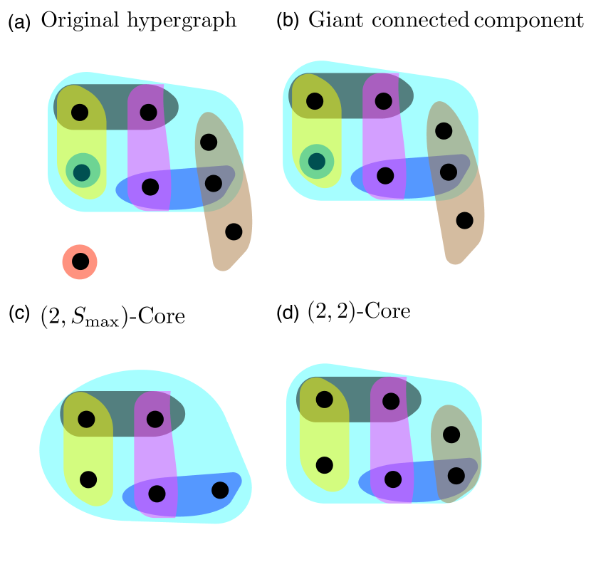
Figure S1: (Color online) Example of the different percolations studied in the work. (a) shows the original hypergraph. (b), (c) and (d) shows the $(2,S_{\max})$-core, $(2,2)$-core, where $S_{\max}\equiv\max(r,2)$ .

II Giant component

A giant connected component of a hypergraph is a connected component that contains a constant fraction of the entire vertices. In the mean-field picture, we can derive a set of self-consistent equations to calculate the relative size of the GCC, using the generating function formalism citeulike:48 . Let $\mu$ represent the probability that a randomly selected vertex from a randomly chosen hyperedge is not connected via other hyperedges with the GCC. Dually, let $\psi$ represent the probability that a randomly chosen hyperedge connecting to a randomly chosen vertex is not connected via other vertices with the GCC. Then we have

$$\mu=\sum_{k=1}^{\infty}Q_{\mathrm{n}}(k)\psi^{k-1}$$ (S1)

$$\psi=\sum_{r=1}^{\infty}Q_{\mathrm{h}}(r)\mu^{r-1}.$$ (S2)

Here $Q_{\mathrm{n}}(k)\equiv kP_{\mathrm{n}}(k)/c$ is the excess degree distribution of vertices, i.e., the degree distribution for the vertices in a randomly chosen hyperedge. $P_{\mathrm{n}}(k)$ is the vertex degree distribution, and $c=c_{1}$ is the mean degree of the vertices. In general we define $c_{m}\equiv\sum_{k=0}^{\infty}k^{m}P_{\mathrm{n}}(k)$. $Q_{\mathrm{h}}(r)\equiv rP_{\rm h}(r)/d$ is the excess cardinality distribution of hyperedges, i.e., the cardinality distribution for the hyperedges connected to a randomly chosen vertex. $P_{\rm h}(r)$ is the hyperedge cardinality distribution, and $d=d_{1}$ is the mean cardinality of the hyperdges. In general we define $d_{m}\equiv\sum_{r=0}^{\infty}r^{m}P_{\rm h}(r)$.

The relative size of the GCC is then given by

$$s_{\mathrm{g}}=1-\sum_{k=0}^{\infty}P_{\mathrm{n}}(k)\psi^{k}.$$ (S3)

Fig. S2 shows the analytical result of $s_{\mathrm{g}}$ as a function of the mean degree $c$ for hypergraphs with Poisson vertex degree distribution and different hyperedge cardinality distributions. Clearly the giant component in hypergraphs emerges as a continuous phase transition with scaling behavior

$$s_{\mathrm{g}}\sim(c-c^{*})^{\eta}$$ (S4)

for $c-c^{*}\rightarrow 0^{+}$, where $c^{*}$ is the critical value of mean degree (i.e., the percolation threshold) and $\eta$ is the critical exponent associated with the critical singularity.

The condition for the percolation transition can be determined by rewriting Eqs.  S1 as

$$F_{\mathrm{g}}=0,$$ (S5)

where we define

$$F_{\mathrm{g}}\equiv\sum_{k=1}^{\infty}Q_{\mathrm{n}}(k)\psi^{k-1}-\mu.$$ (S6)

At the critical point when $\mu^{*}=1$ and

$$\left.\frac{\partial F_{\mathrm{g}}}{\partial\mu}\right|_{\mu=\mu^{*}=1}=0,$$ (S7)

we obtain

$$\frac{d_{2}-d}{d}\frac{c_{2}-c}{c}>1.$$ (S8)

where $c^{*}$ and $c^{*}_{2}$ are the hyperdegree first and second moment, respectively, at the critical point.

Note that a similar relation has been found for uniform hypergraphs Mezard2009IPC1592967 . In the graph case ($d=2$ for all edges) we recover the classical result $\frac{c_{2}-c}{c}>1$ RevModPhys.80.1275 ; molloyreed95 .

The critical exponent $\eta$ can be calculated by consider a point around the critical point, such as, $\mu=1-\zeta$ with $\zeta=0^{+}$ and $c=c^{*}+\chi$ with $\chi=0^{+}$. We can define the function from Eq.  S6 as a function of $\mu$ and $c$ (i.e. $F_{\mathrm{g}}(\mu,c)$). By expanding $F_{\mathrm{g}}(\mu,c)$ around the point $(\mu,c)=(1,c^{*})$ and combining it with the result from Eq.  S7 at the critical point, we can rewrite Eq. S6 as

$$\left.\frac{\partial F_{\mathrm{g}}(\mu,c)}{\partial c}\right|_{(1,c^{*})}\chi+\left.\frac{\partial^{2}F_{\mathrm{g}}(\mu,c)}{\partial^{2}\mu}\right|_{(1,c^{*})}\zeta^{2}+\left.\frac{\partial^{2}F_{\mathrm{g}}(\mu,c)}{\partial^{2}c}\right|_{(1,c^{*})}\chi^{2}$$ (S9)

$$-2\left.\frac{\partial^{2}F_{\mathrm{g}}(\mu,c)}{\partial\mu\partial c}\right|_{(1,c^{*})}\chi\zeta+(\cdot\cdot\cdot)=0.$$

For $\mu=1$,

$$F_{\mathrm{g}}(1,c)=1-c/c=0,$$ (S10)

it follows that

$$\left.\frac{\partial^{n}F_{\mathrm{g}}(\mu,c)}{\partial^{n}c}\right|_{(1,c^{*})}=0$$ (S11)

for any positive integer $n$. Let us assume that there are no diverging moments for the hyperedge cardinality distribution. We can truncate our expansion of $F_{\mathrm{g}}$ at order 2 for $\zeta$ and $\chi$. This implies that

$$\zeta\sim\chi.$$ (S12)

Let us expand $s_{g}$ as a function of $\zeta$,

$$s_{g}=\left.s_{g}(\mu)\right|_{\mu=\mu^{*}}-\left.\frac{\partial s_{g}(\mu)}{\partial\mu}\right|_{\mu=\mu^{*}}\zeta+\left.\frac{\partial^{2}s_{g}(\mu)}{\partial^{2}\mu}\right|_{\mu=\mu^{*}}\zeta^{2}+(\cdot\cdot\cdot).$$ (S13)

For $\mu^{*}=1$, $s_{g}(\mu^{*})=0$. We obtain

$$s_{{}_{\mathrm{g}}}\sim\chi,$$ (S14)

This correspond to he same exponent $\eta=1$ as in the graph case RevModPhys.80.1275 ; Bollobás2013 .

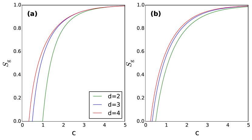
Figure S2: (Color online) The relative size of the GCC $s_{\mathrm{g}}$ as a function of the mean degree $c$ for hypergraphs with Poisson vertex degree distribution. (a) $d$-uniform hypergraphs with $d=2,3,4$; (b) hypergraphs with Poisson hyperedge cardinality distribution and mean cardinality $d=2,3,4$.

III $(K,S)$-core on hypergraphs

The $(K,S)$-core of a hypergraph is obtained by recursively removing vertices with degree less than $K$ and hyperedge with cardinality less than $S$. A hyperedge with cardinality $r$ is removable if at least $r-S+1$ vertices connected to it are also removable and a vertex with degree $k$ is removable if at least $k-K+1$ hyperedges connected to it are also removable. One can remove a vertex or a hyperedge from the hypergraph, and see what is the probability of a neighboring hyperedge or vertex, respectively, being removable. This allows us to derive a set of self-consistent equations:

$$\alpha=\sum_{k=1}^{\infty}Q_{\mathrm{n}}(k)\sum_{l=k+1-S}^{k-1}\left(\begin{array}[]{c}k-1\\ l\end{array}\right)\delta^{l}(1-\delta)^{k-1-l},$$ (S17)

$$\delta=\sum_{r=1}^{\infty}Q_{\mathrm{h}}(r)\sum_{l=r+1-K}^{r-1}\left(\begin{array}[]{c}r-1\\ l\end{array}\right)\alpha^{l}(1-\alpha)^{r-1-l}.$$ (S20)

Here $\alpha$ and $\delta$ are, respectively, the probability that a vertex or a hyperedge is removable. From now on we will focus on the case of $K=2$. Then Eq. (S17) reduces to

$$\alpha=\sum_{k=1}^{\infty}Q_{\mathrm{n}}(k)\delta^{k-1}.$$ (S21)

III.1 $K=2$ and $S=S_{\max}$

The $(K,S)$-core defined with $K=2$ and $S=S_{\max}\equiv\max(r,2)$, (where $S_{\max}=2$ if $r<2$ and and $S_{\max}=r$ if $r\geq 2$ and $r$ is the intial cardinality of an hyperedge before any removal process) is obtained by recursively removing all vertices with degree one as well as the hyperedges containing them, and all hyperedges with cardinality smaller than two. Hyperedges with cardinality one or zero do not connect any nodes, thus have no meaning in what cores are concerned. In this case the threshold $S$ depends on the cardinally of the hyperedges. Furthermore, if one of the vertices of any hyperedge is removed the hyperedge is also removed. (Note that the $(2,S_{\max})$-core has been defined in literature Cooper03thecores simply as $2$-core, and discontinuous $2$-core percolation is found in $d$-uniform hypergraphs with $d>2$.) In this case, Eq. (S20) reduces to

$$1-\delta=\sum_{r=2}^{\infty}Q_{\mathrm{h}}(r)(1-\alpha)^{r-1}.$$ (S22)

The relative size of the $(2,S_{\mathrm{max}})$-core is given by the probability that a randomly chosen vertex is connected to at least two non-removable hyperedges:

$$s_{\mathrm{2c}}=\sum_{k=2}^{\infty}P_{\rm h}(k)\sum_{l=2}^{k}\left(\begin{array}[]{c}k\\ l\end{array}\right)(1-\delta)^{l}\delta^{k-l}.$$ (S23)

Fig. S3 shows the analytical result of $s_{\mathrm{2c}}$ as a function of the mean degree $c$ for hypergraphs with Poisson vertex degree distribution and different hyperedge cardinality distributions.

Figure S3: (Color online) The relative size of $(2,S)$-core $s_{\mathrm{2c}}$ as a function of the mean degree $c$ for hypergraphs with Poisson degree distribution, for $S=\max(r-1,2)$ (a) and (b), and $S=2$, (b) and (d). (a) and (c) $d$-uniform hypergraphs . (b) and (d) hypergraphs with Poisson hyperedge cardinality distribution.

We find that, depending on the mean hyperedge cardinality $d$, the $(2,S_{\max})$-core emerges as either a continuous or a hybrid phase transition, with scaling behavior

$$s_{\mathrm{2c}}-s_{\mathrm{2c}}^{*}\sim(c-c^{*})^{\zeta}$$ (S24)

for $c-c^{*}\to 0^{+}$, where $c^{*}$ is the percolation threshold and $\zeta$ is the critical exponent. $s_{\mathrm{2c}}^{*}$ is the $(2,S_{\mathrm{max}})$-core relative size right at the critical point: $s_{\mathrm{2c}}^{*}=0$ for continuous phase transition and non-zero for hybrid phase transitions. The percolation threshold $c^{*}$ can be calculated by defining

$$F_{\mathrm{2c}}\equiv\sum_{k=1}^{\infty}Q_{\mathrm{n}}(k)\delta^{k-1}-\alpha=0.$$ (S25)

If we consider $S=\max(r,2)$, $\delta$, defined in Eq. S22, and we combine Eqs. S25,  S29 and S22, we obtain

$$1=\sum_{k=1}^{\infty}\sum_{r=2}^{\infty}Q^{*}_{\mathrm{n}}(k)Q_{\mathrm{h}}(r)(k-1)(r-1){\delta^{*}}^{k-2}(1-\alpha^{*})^{r-2},$$ (S26)

where $Q^{*}_{\mathrm{n}}(k)$ is the connectivity distribution with the critical mean hyperdegree $c^{*}$. $\delta^{*}$ and $\alpha^{*}$ are the values of $\delta$ and $\alpha$ at the critical point, respectively. The phase transition is continuous if for $\delta^{*}=\alpha^{*}=1$,

$$\left.\frac{\partial^{2}F_{\mathrm{2c}}}{\partial^{2}\alpha}\right|_{\alpha=1}>0,$$ (S27)

that reduces to,

$$2Q_{\mathrm{n}}(3)(c^{*}_{2}-c^{*})-Q_{\mathrm{n}}(2)^{2}(c^{*}_{3}-3c^{*}_{2}+2c^{*})<0.$$ (S28)

where $c^{*}_{3}$ and $c^{*}_{2}$ is third and second moment of the degree distribution at the critical point, respectively. The phase transition is only continuous if at the critical point

$$\left.\frac{\partial F_{\mathrm{2c}}}{\partial\alpha}\right|_{(\alpha,c_{1})=(\alpha^{*},c^{*})}=0.$$ (S29)

From this condition we obtain that the critical point for a continuous phase transition is given by,

$$Q_{\mathrm{h}}(2)\frac{c^{*}_{2}-c^{*}}{c^{*}}=1.$$ (S30)

Let us assume a Poisson distribution of hyperdegrees, in this case $c^{*}_{2}-c^{*}={c^{*}}^{2}$ and $c^{*}_{3}-3c^{*}_{2}+2c^{*}={c^{*}}^{2}$. Combine these relations with Eqs. S28 and S30, Eq. S30 reduces to

$$2Q_{\mathrm{h}}(3)<Q_{\mathrm{h}}(2).$$ (S31)

If the hyperedge cardinality follows a Poisson distribution, there is a continuous phase transition when $d_{1}<1$, witch corresponds to

$$d_{1}<\bar{d},$$ (S32)

where $\bar{d}\equiv 1$. Let us consider points around the critical point, such as $\alpha=\alpha^{*}-\zeta$ with $\zeta=0^{+}$ and $c=c^{*}+\chi$ with $\chi=0^{+}$. We can define the function from Eq. S25 as a function of $\alpha$ and $\chi$ (i.e. $F_{\mathrm{2c}}(\alpha,c)$). By expanding $F_{\mathrm{g}}(\alpha,\chi)$ around the point $(\alpha,c)=(\alpha^{*},c^{*})$ and combining it with result from Eq S29 at the critical point, we can rewrite Eq. S6 as

$$\left.\frac{\partial F_{\mathrm{2c}}(\alpha,c)}{\partial c}\right|_{(\alpha^{*},c^{*})}\chi+\left.\frac{\partial^{2}F_{\mathrm{2c}}(\alpha,c)}{\partial^{2}\alpha}\right|_{(\alpha^{*},c^{*})}\zeta^{2}+\left.\frac{\partial^{2}F_{\mathrm{2c}}(\alpha,c_{1})}{\partial^{2}c}\right|_{(\alpha^{*},c^{*})}\chi^{2}-2\left.\frac{\partial^{2}F_{\mathrm{2c}}(\alpha,c)}{\partial\alpha\partial c}\right|_{(\alpha^{*},c^{*})}\chi\zeta+(\cdot\cdot\cdot)=0.$$ (S33)

For the continuous phase transition, $\alpha^{*}=1$, this implies

$$\left.\frac{\partial^{n}F_{\mathrm{2c}}(\mu,c_{1})}{\partial^{n}c}\right|_{(1,c^{*})}=0$$ (S34)

for any positive integer $n$. Thus,

$$\zeta\sim\chi.$$ (S35)

Let us expand $s_{2c}$ as a function of $\zeta$,

$$s_{2c}=\left.s_{2c}(\mu)\right|_{\alpha=\alpha^{*}}-\left.\frac{\partial s_{2c}(\alpha)}{\partial\alpha}\right|_{\alpha=\alpha^{*}}\zeta+\left.\frac{\partial^{2}s_{2c}(\alpha)}{\partial^{2}\alpha}\right|_{\alpha=\alpha^{*}}\zeta^{2}+(\cdot\cdot\cdot),$$ (S36)

For $\alpha^{*}=1$, $s_{2c}(\alpha^{*})=0$ and

$$\left.\frac{\partial s_{2c}(\alpha)}{\partial\alpha}\right|_{\alpha=\alpha^{*}=1}=0.$$ (S37)

We obtain

$$s_{2c}\sim\zeta^{2}\Rightarrow s_{2c}\sim\chi^{2},$$ (S38)

for $s_{2c}^{*}=0$ and $\eta=2$. For the discontinuous phase transition, $\alpha^{*}\neq 1$, we have

$$\left.\frac{\partial F_{\mathrm{2c}}(\alpha,c)}{\partial c}\right|_{(1,c^{*})}\neq 0,$$ (S39)

$s_{2c}(\alpha)\neq 0$ and

$$\left.\frac{\partial s_{2c}(\alpha)}{\partial\alpha}\right|_{\alpha=\alpha^{*}}\neq 0.$$ (S40)

It implies

$$\zeta\sim\chi^{1/2},$$ (S41)

and

$$s_{2c}-s^{*}_{2c}\sim\chi^{1/2},$$ (S42)

that is equivalent to Eq. S24 for $\eta=1/2$. A discontinuous phase transition with a critical exponent smaller than one is considered as hybrid phase transition.

At the critical mean cardinality, $d=\bar{d}$, $\alpha^{*}=1$, but

$$\left.\frac{\partial^{2}F_{\mathrm{2c}}}{\partial^{2}\alpha}\right|_{\alpha=1}=0.$$ (S43)

In this case we have to take into account terms of order $3$ in the expansion of Eq. S33. We obtain,

$$\zeta\sim\chi^{1/2},$$ (S44)

and,

$$s_{2c}\sim\chi,$$ (S45)

We can summarize that for $d$-uniform hypergraphs the $(2,S_{\mathrm{max}})$-core percolation is (i) continuous with critical exponent $\zeta=2$ if $d=2$; and (ii) hybrid with critical exponent $\zeta=1/2$ if $d>2$ (which is consistent with a previous work Cooper03thecores ). For hypergraphs where both the vertex degeree and hyperedge cardnality distributions are Poissonian, the $(2,\max(r,2))$-core percolation is (i) continuous with critical exponent $\zeta=2$ if $d<\bar{d}=1$; (ii) continous with critical exponent $\zeta=1$ if $d=\bar{d}$; and (iii) hybrid with critical exponent $\zeta=1/2$ if $d>\bar{d}$. The same set of critical exponents was found for the heterogeneous-$K$-core PhysRevLett.107.175703 .

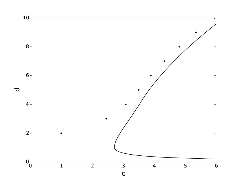
Figure S4: Phase diagram of $(2,\max(r,2))$-core percolation on hypergraphs with Poisson vertex degree distributions. Black circles and black line represents the phase boundary of $d$-uniform hypergraphs and hypergraphs with Poisson hyperedge cardinality distribution, respectively.

III.2 $K=2$ and $S=2$

In this section we study the $(2,2)$-core. A similar definition of removable hyperedges was used in citeulike:11962060 , where the core obtained from the GLR procedure is used to study the vertex cover problem in uniform hypergraphs.

In this case, Eq. (S20) reduces to

$$\delta=\sum_{r=1}^{\infty}Q_{\mathrm{h}}(r)\alpha^{r-1}.$$ (S46)

The relative size of the $(2,2)$-core can be calculated by considering the probability that a randomly chosen vertex is connected to at least two non-removable hyperedges and the probability that a degree-one vertex is connected to a hyperedge with less than $(r-2)$ other degree-one vertices. This results in

$$s_{\mathrm{2c}}=\sum_{k=2}^{\infty}P_{\mathrm{n}}(k)\sum_{l=2}^{k}\binom{k}{l}(1-\delta)^{l}\delta^{k-l}.$$ (S47)

Eqs. (S23) and (S46) have the same critical point as Eqs. (S21) and (S20). Therefore, for $(2,2)$-core we recover the result found in the graph case that both the $(2,2)$-core and the GCC emerge at the same critical point RevModPhys.80.1275 . We can compute the critical point by combining Eq. S25, S46 and S34 at $\alpha=\delta=1$, obtaining

$$\frac{d_{2}-d_{1}}{d_{1}}\frac{c^{*}_{2}-c^{*}}{c^{*}}=1,$$ (S48)

In this case the phase transition is always continuous (see solid lines in Fig. S3 c and d) and for the studied hyperedge cardinality and vertex degree distributions we have $\eta=2$.

As before, we assume that the moments of the vertex degree and hyperedge cardinality distributions do not diverge. Let us consider points around the critical point, such as, $\alpha=1-\zeta$ with $\zeta=0^{+}$ and $c=c^{*}+\chi$ with $\chi=0^{+}$. We can define the function from Eqs. S25 as a function of $\alpha$ and $\chi$( i.e. $F_{\mathrm{2c}}(\alpha,c)$). By expanding $F_{\mathrm{g}}(\alpha,\chi)$ around the point $(\alpha,c)=(1,c^{*})$, and combining it with result from Eq. S29 at the critical point, we can rewrite Eq. S6 as

$$\left.\frac{\partial^{2}F_{\mathrm{2c}}(\alpha,c)}{\partial^{2}\alpha}\right|_{(1,c^{*})}\zeta^{2}-2\left.\frac{\partial^{2}F_{\mathrm{2c}}(\alpha,c)}{\partial\alpha\partial c}\right|_{(1,c^{*})}\chi\zeta+(\cdot\cdot\cdot)=0.$$ (S49)

Note that for this case the Eq. S34 is still valid. We obtain

$$\zeta\sim\chi.$$ (S50)

By combining this equations with the fact that $s_{2c}(\alpha^{*})=0$ and the result from Eq. S37, we obtain

$$s_{2c}\sim\chi^{2}.$$ (S51)

IV Core percolation on hypergraphs

In Sec. IV.1 we show the relation between the hyperedge covering problems and the dominating set problem Sec. IV.1 We also show how our algorithm is a generalization of the greedy leaf removals procedure Zhao2015 used to solve the dominant set problem in polynomial time, and that the core obtain trough our methodology is always smaller than produced by the greedy leaf removal. In Sec. IV.2 to Sec. IV.5 we show the detailed derivations for the equations in the main text.

IV.1 Relation between hyperedge and vertex covering problems and the minimum dominating set problem

The minimum dominating set (MDS) is the smallest set of vertices, $D$ of a graph $G$, so that every vertex in $G$ is adjacent to at least one vertex in $D$. The MDS can be mapped to a minimum hyperedge cover in a hypergraph composed by the same vertices as in $G$ and for each vertex $v_{1}$ there is an hyperedge, $h_{1}$, that contains $v_{1}$ and all neighbors of $v_{1}$ (see Figure S5). Therefore if we find the set of hyperedges $[v_{i},...,v_{j}]$, that covers all vertices in this hypergraph, the dominanting set of graph $G$ is given by $[v_{i},...,v_{j}]$. Our method is a generalization of the method proposed in Zhao2015 . Note that our method doesn’t focus onleaves, i.e., vertices with degree one. As shown in Figure S5, even given the fact that there is no one-degree vertices, our method can still solve the MDS exactly in polynomial time.

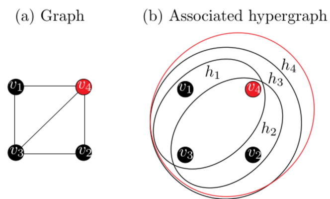
Figure S5: A graph and the associated hypergraph. Hyperedge $h_{i}$ represents vertices observed by vertice $v_{i}$. Solving the hypergraph’s minimum hyperedge cover set is equivalent to solve the graph’s dominating set. The red vertex represents the solution of the minimum dominating set problem in graph (a), the red edge the solution of the minimum hyperedge cover set problem.

We emphasize that the greedy leaf removals rules described in Zhao2015 are special cases of our method. Let us consider the first rule: if vertex $v_{i}$ is an unobserved leaf vertex (which has only a single neighbor, say $v_{j}$), then occupying $v_{j}$ but leaving $v_{i}$ empty must be an optimal strategy. And let us now consider the hypergraph with the same nodes as the original graph, and hyperedges $h_{i}$ that represent the vertices observed by node $v_{i}$. For a leaf $v_{i}$ the set of vertices that are covered by hyperedge $h_{i}$ is a subset or equal set to the ones covered by hyperedge $h_{j}$, i.e. $V_{i}\subseteq V_{j}$, then $h_{i}$ can be removed. After this, the hyperedges that cover $v_{i}$ are a subset of or equal to the set of hyperedges that cover $h_{j}$ ($H_{i}\subseteq H_{j}$), and a subset or equal set of hyperedges that cover the other neighbors of $v_{j}$, in the original network, $v_{k}$ ($H_{i}\subseteq H_{k}$). Then vertices $v_{j}$ and $v_{k}$ are removed. Note that all observed nodes are removed from the network, in our method, since they do not need to be observed anymore, but we still keep the hyperedges associated with them because they can still be used to cover other vertices. After this process the cardinality of hyperedge $h_{j}$ is one, meaning that $h_{j}$ is part of a minimum hyperedge cover set. In terms of dominating set it means that occupying node $j$ is an optimal strategy. Let us now consider the second rule : if vertex $v_{i}$ is an unobserved leaf vertex (which has only a single neighbor, say $v_{j}$), then occupying $v_{j}$ but leaving $v_{i}$ empty must be an optimal strategy, and if $v_{i}$ is an empty but observed vertex and at most one of its adjacent vertices is unobserved, then it must be an optimal strategy not to occupy $v_{i}$. We emphasize that in our hyperedge all observed vertices $v_{k}$ are automatically removed from the network. If all except at most one neighbor of vertex $i$ is unobserved,$v_{j}$, then $h_{i}$ can also be removed because all vertices covered by hyperedge $v_{i}$ are also covered by vertex, $v_{j}$ ($H_{i}\subseteq H_{j}$). In terms of dominating set it means that not occupying vertice $v_{i}$ is an optimal strategy.

Table 1 shows the size of the cores associated with the dominating set, for the eleven networks analyzed in Zhao2015 . For most networks our method shows a considerable improvement, . For some of them, our method actually find no core left.

Networks	$N$	$M$	$s_{\rm glr}$	$s_{\rm d}$
RoadEU	1177	1417	0.260	0.167
PPI	2361	6646	0.007	0.000
Grid	4941	6594	0.122	0.056
IntNet1	6474	12572	0.001	0.000
Author	23133	93439	0.391	0.000
Citation	34546	420877	0.326	0.310
P2P	62586	147892	0.001	0.000
Friend	196591	950327	0.031	0.001
Email	265214	364481	0.002	0.000
Webpage	875713	4322051	0.185	0.004
RoadTX	1379917	1921660	0.406	0.342

Table 1: Normalized size of the cores associated with the minimum dominanting set problem for eleven real-world networka, using the greedy leaf removal procedure fromZhao2015 , $s_{\rm glr}$, and using our approach $s_{\rm d}$. $N$ and $M$ are, respectively, the total number of nodes and links in the network.

IV.2 Number of hyperedges contained in the core

In the main text we characterize the size of the core as the number of vertices contained in the core, we can also compute the number of hyperedges in each core, $s^{\prime}_{v}$ and $s^{\prime}_{h}$. We can use the fact that the v_core of a hypergraph is h_core of the dual hypergraph. Thus, we can get Eqs. (1) (2) (7) and (8) in the main text by the following transformation

$$\alpha\rightarrow\delta$$ (S52)

$$\delta\rightarrow\beta$$ (S53)

$$\beta\rightarrow\epsilon$$ (S54)

$$\epsilon\rightarrow\alpha$$ (S55)

on Eqs. (1) to (4) from the main text. Because the vertices of an hypergraph are hyperedges in the dual one, we obtain that $s^{\prime}_{\rm h}$ is given by

$$s^{\rm h}_{\mathrm{h}}=\sum_{k=2}^{\infty}P_{\mathrm{h}}(r)\sum_{l=2}^{k}\binom{k}{l}(1-\beta-\alpha)^{l}\alpha^{k-l},$$ (S56)

where $\alpha$, $\beta$ ,$\delta$ and $\gamma$ are obtained by solving Eqs. (1),(2) (7) and (8) in the main text. Using the same argument we can conclude that $s^{\prime}_{h}$ is given by

$$s^{\rm h}_{\mathrm{v}}=\sum_{k=2}^{\infty}P_{\mathrm{h}}(r)\sum_{l=2}^{k}\binom{k}{l}(1-\alpha-\beta)^{l}\beta^{k-l},$$ (S57)

where $\alpha$, $\beta$ ,$\delta$ and $\gamma$ are obtained by solving Eqs. (1),(2) (7) and (8) in the main text.

IV.3 $v_{\rm core}$ for uniform hypergraphs - critical point

There is a simple relation between $v_{\rm core}$ critical point and the mean cardinality $d_{1}$ for uniform hypergraphs with $d_{1}>1$. Let us start by rewriting Eq. 1 in the main text as

$$F_{\mathrm{c1}}(\alpha,c)=0$$ (S58)

where we define

$$F_{\mathrm{c1}}(\alpha,c)\equiv\sum_{k=1}^{\infty}Q_{\mathrm{n}}(k)\epsilon^{k-1}-\alpha.$$ (S59)

For uniform-Poisson hypergraph Eqs (1), (2) and (7) and (8) in the main text can be reduced to

$$x =e^{-c(d_{1}-1)y}$$ (S60)

$$y =e^{-c(d_{1}-1)x},$$ (S61)

where we define $x\equiv\alpha^{r-1}$ and $y\equiv(1-\beta)^{r-1}$. The function defined in Eq. S59 can be written as a function of $x$ and $c$,

$$F_{\mathrm{c1}}(x,c)\equiv\exp{\left(-c~{}(d_{1}-1)~{}e^{-c~{}(d_{1}-1)~{}x}\right)}-x.$$ (S62)

The critical point is given by $\alpha^{*}=(c^{*}~{}(d_{1}-1))^{1/(1-d_{1})}$ and $c^{*}=e/(d_{1}-1)$.

IV.4 $v_{\rm core}$ - critical exponent

Eqs. 1 and 2, 7 and 8 in the main text can be written as

$$\alpha =A(1-z)$$ (S63)

$$z =B(h)$$ (S64)

$$h =A(1-\delta)$$ (S65)

$$\delta =B(\alpha)$$ (S66)

where we define $z\equiv 1-\epsilon$, $h\equiv 1-\beta$, $A(1-z)\equiv\sum_{k=1}^{\infty}Q_{\mathrm{n}}(k)(1-z)^{k-1}$ and $\left.B(h)\equiv\sum_{r=2}^{+\infty}Q_{r}(r)h^{r-1}\right.$. $F_{\mathrm{v}}(\alpha,c)$ can be written as

$$F_{\mathrm{v}}(\alpha,c)=H(H(\alpha,c),c)-\alpha,$$ (S67)

where we define

$$H(\alpha,c)\equiv A(1-B(\alpha),c1).$$ (S68)

This function has the same form for the graph case, (see Eq. S60 from PhysRevLett.109.205703 ). The only difference is the way we define the function $H(\alpha,c)$. Nevertheless it obeys the same relation, and therefore has the same critical exponent $\zeta_{1}=1$, i.e:

$$\left.\frac{\partial H(\alpha,c)}{\partial\alpha}\right|_{(\alpha,c)=(\alpha^{*},c^{*})}=-1,$$ (S69)

$$\left.\frac{\partial F_{\mathrm{h}}(\alpha,c)}{\partial c}\right|_{(\alpha,c)=(\alpha^{*},c^{*})}=0,$$ (S70)

$$\left.\frac{\partial^{2}F_{\mathrm{h}}(\alpha,c)}{\partial^{2}\alpha}\right|_{(\alpha,c)=(\alpha^{*},c^{*})}=0.$$ (S71)

From an expansion of $F_{\mathrm{h}}$ as a function of $(c-c^{*})$, for $c-c^{*}=0^{+}$, it follows that

$$\alpha-\alpha^{*}\sim(c-c^{*})^{1/2},$$ (S72)

$$\beta-\beta^{*}\sim(c-c^{*})^{1/2},$$ (S73)

$$1-\beta-\alpha\sim(c-c^{*})^{1/2},$$ (S74)

and

$$s^{\rm v}_{v}\sim(c-c^{*}),$$ (S75)

witch is equivalent to Eq. (6) in the main text, for $\zeta_{1}=1$.

IV.5 $h_{\rm core}$ - critical exponent

Eqs. (1) to (4) in the main text can be written as

$$\alpha =A(\epsilon)$$ (S76)

$$\epsilon =B(1-u)$$ (S77)

$$u =A(v)$$ (S78)

$$v =B(1-\alpha)$$ (S79)

where we define $u\equiv 1-\beta$ and $v\equiv 1-\delta$. The function $F_{\mathrm{c2}}(\alpha,c)\equiv A(\epsilon,c)-\alpha$ can be written as

$$F_{\mathrm{h}}(\alpha,c)=G(G(\alpha,c),c)-\alpha,$$ (S80)

where we define

$$G(\alpha,c)\equiv A(B(1-u),c1).$$ (S81)

This function has the same form as Eqs. S68. The only difference is how we define the function $G(\alpha,c)$. Nevertheless it obeys the same relations as Eqs. S69 to S74, thus,

$$s^{\rm v}_{\rm h}\sim(c-c^{*})^{\zeta_{2}},$$ (S82)

with $\zeta_{2}=\zeta_{1}=1$.

V Simulations

We compare our analytical calculations with random hypergraphs generated in the following ways.

V.0.1 Poisson-Uniform hypergraphs

We first generate random hypergraphs where all hyperedges have the same cardinality $d$ and the vertex hyperdegrees follow a Possion distribution with average value $c_{1}$. We can generate this hypergraphs by creating $N$ nodes and $L$ hyperedges of cardinality $d$. We then fill the hyperedges with random selected vertices from our list of nodes. In the end

$$c=dL/N.$$ (S83)

V.0.2 Poisson-Poisson hypergraphs

In the Poisson-Poisson hypergraphs we generate random hypergraphs where and both the vertex degrees and hyperedge cardinalities follow a Possion distribution with average $c$ (or $d$), respectively. We can generate this hypergraphs by creating $N$ vertices and $L$ hyperedges. We then select random vertices and add it to a random selected hyperedge until the average hyperdegree of the network is

$$c=d\times L/N.$$ (S84)

V.1 Results

Figures S6 to S10 show that numerical simulations agree well with the analytical calculations. In the simulations we used hypergraphs of size $10^{4}$ vertices.

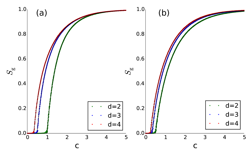
Figure S6: The relative size of the giant connected component, $s_{\mathrm{g}}$, for hypergraphs with Poisson vertex degree distributions and mean degree $c$. Black solid lines: theoretical results. Dots: numerical results from hypergraphs with $10^{4}$ vertices. (a) $d$-uniform hypergraphs where all hyperdege have the same cardinality $d$. (b) the hyperedge cardinality follows a Poisson distribution with average cardinality $d$.

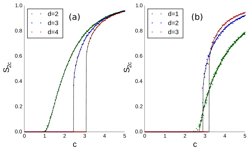
Figure S7: (a) The relative size of the $(2,S)$-core with $S=\max\left(r-1,2\right)$ for hypergraphs with Poisson vertex degree distributions and mean degree $c$. Black solid lines: theoretical results. Dots: numerical results from hypergraphs with $10^{4}$ vertices. (a) $d$-uniform hypergraphs where all hyperdege have the same cardinality $d$. (b) the hyperedge cardinality follows a Poisson distribution with average cardinality $d$.

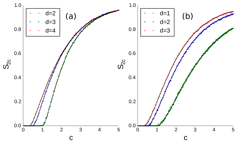
Figure S8: The relative size of the $(2,S)$-core with $S=2$ for hypergraphs with Poisson vertex degree distributions and mean degree $c$. Black solid lines: theoretical results. Dots: numerical results from hypergraphs with $10^{4}$ vertices. (a) $d$-uniform hypergraphs where all hyperdege have the same cardinality $d$. (b) the hyperedge cardinality follows a Poisson distribution with average cardinality $d$.

Figure S9: $h_{\rm core}$ obtained from simulations. The relative size of the h-core for hypergraphs with Poisson vertex degree distributions and mean degree $c$. Black solid lines: theoretical results. Dots: numerical results from hypergraphs with $10^{5}$ vertices. (a) $d$-uniform hypergraphs where all hyperdege have the same cardinality $d$. (b) the hyperedge cardinality follows a Poisson distribution with average cardinality $d$.

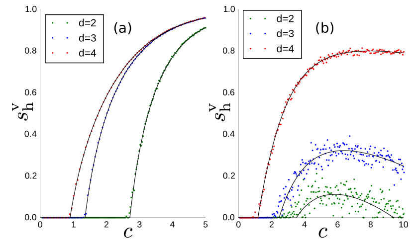
Figure S10: $v_{\rm core}$ obtained from simulations. The relative size of the v-core for hypergraphs with Poisson vertex degree distributions and mean degree $c$. Black solid lines: theoretical results. Dots: numerical results from hypergraphs with $10^{5}$ vertices. (a) $d$-uniform hypergraphs where all hyperdege have the same cardinality $d$. (b) the hyperedge cardinality follows a Poisson distribution with average cardinality $d$. The large fluctuation for $d=2$ and $3$ are due to the relatively large number of hypereges with cardinalty $1$, and the chance that if a edge is connected to a hypereges with cardinalty $1$ is automatically removed.

VI Contributions and Author Information

Contributions. Y.-Y.L. and H.-J.Z conceived the project. All authors designed the research. B.C.C. performed all the analytical calculations and numerical simulations. All authors analyzed the results. B.C.C. and Y.-Y.L. wrote the manuscript. H.-J.Z. edited the manuscript.

Author Information. The authors declare no competing financial interests. Correspondence and requests for materials should be addressed to Y.-Y.L. (yyl@channing.harvard.edu), or B.C.C. (coutinho.b@husky.neu.ed).

References

- [1] Christina Goldschmidt. Critical random hypergraphs: the emergence of a giant set of identifiable vertices. Ann/ Prob, pages 1573–1600, 2005.
- [2] Colin Cooper. The cores of random hypergraphs with a given degree sequence. Random Structures and Algorithms, 25(4):353–375, 2004.
- [3] Satoshi Takabe and Koji Hukushima. Minimum vertex cover problems on random hypergraphs: Replica symmetric solution and a leaf removal algorithm. Phys. Rev. E, 89:062139, Jun 2014.
- [4] S. N. Dorogovtsev, A. V. Goltsev, and J. F. F. Mendes. k-core organization of complex networks. Phys. Rev. Lett., 96:040601, Feb 2006.
- [5] J. Ignacio Alvarez-hamelin, Alain Barrat, and Alessandro Vespignani. Large scale networks fingerprinting and visualization using the k-core decomposition. In Advances in Neural Information Processing Systems 18, pages 41–50. MIT Press, 2006.
- [6] S. N. Dorogovtsev, A. V. Goltsev, and J. F. F. Mendes. Critical phenomena in complex networks. Rev. Mod. Phys., 80:1275–1335, Oct 2008.
- [7] P. Erdös and A. Rényi. On random graphs, I. Publicationes Mathematicae (Debrecen), 6:290–297, 1959.
- [8] Maksim Kitsak, Lazaros K. Gallos, Shlomo Havlin, Fredrik Liljeros, Lev Muchnik, H. Eugene Stanley, and Hernan A. Makse. Identification of influential spreaders in complex networks. Nat Phys, 6(11):888–893, 11 2010.
- [9] M. Bauer and O. Golinelli. Exactly solvable model with two conductor-insulator transitions driven by impurities. Phys. Rev. Lett., 86:2621–2624, Mar 2001.
- [10] Yang-Yu Liu, Jean-Jacques Slotine, and Albert-Laszlo Barabasi. Controllability of complex networks. Nature, 473(7346):167–173, May 2011.
- [11] Richard M. Karp and M. Sipser. Maximum matching in sparse random graphs. In Foundations of Computer Science, 1981. SFCS ’81. 22nd Annual Symposium on, pages 364–375, Oct 1981.
- [12] M. E. J. Newman, S. H. Strogatz, and D. J. Watts. Random graphs with arbitrary degree distributions and their applications. Phys. Rev. E, 64:026118, Jul 2001.
- [13] Marc Mezard and Andrea Montanari. Information, Physics, and Computation. Oxford University Press, Inc., New York, NY, USA, 2009.
- [14] Michael Molloy and Bruce Reed. A critical point for random graphs with a given degree sequence. Random Structures and Algorithms, 6:161–179, 1995.
- [15] Béla Bollobás and Oliver Riordan. Erdős Centennial, chapter The Phase Transition in the Erdős-Rényi Random Graph Process, pages 59–110. Springer Berlin Heidelberg, Berlin, Heidelberg, 2013.
- [16] Davide Cellai, Aonghus Lawlor, Kenneth A. Dawson, and James P. Gleeson. Tricritical point in heterogeneous k-core percolation. Phys. Rev. Lett., 107:175703, Oct 2011.
- [17] Jin-Hua Zhao, Yusupjan Habibulla, and Hai-Jun Zhou. Statistical mechanics of the minimum dominating set problem. Journal of Statistical Physics, 159(5):1154–1174, 2015.
- [18] Yang-Yu Liu, Endre Csóka, Haijun Zhou, and Márton Pósfai. Core percolation on complex networks. Phys. Rev. Lett., 109:205703, Nov 2012.