Short-time elasticity of polymer melts: Tobolsky conjecture and heterogeneous local stiffness

SEBASTIANO BERNINI¹, DINO LEPORINI^1,2

¹Dipartimento di Fisica “Enrico Fermi”, Università di Pisa, Largo B.Pontecorvo 3, I-56127 Pisa, Italy
²IPCF-CNR, UOS Pisa, Italy

Dated:

ABSTRACT: An extended Molecular-Dynamics study of the short-time ”glassy” elasticity exhibited by a polymer melt of linear fully-flexible chains above the glass transition is presented. The focus is on the infinite-frequency shear modulus $G_{\infty}$ manifested in the picosecond time scale and the relaxed plateau $G_{p}$ reached at later times and terminated by the structural relaxation. The local stiffness of the interactions with the first neighbours of each monomer exhibits marked distribution with average value given by $G_{\infty}$. In particular, the neighbourhood of the end monomers of each chain are softer than the inner monomers, so that $G_{\infty}$ increases with the chain length. $G_{p}$ is not affected by the chain length and is largely set by the non-bonding interactions, thus confirming for polymer melts the conjecture formulated by Tobolsky for glassy polymers.

Keywords: Elasticity, Polymer melt, Molecular-Dynamics simulation

INTRODUCTION

Above the glass transition (GT) the elastic response of uncrosslinked polymer melts $G(t)$ is transient and disappears due to relaxation and viscous effects ¹. The decay of $G(t)$ is characterised by several regimes. In the picosecond time scale, $G(t)\simeq G_{\infty}$ and the elastic deformation is homogeneous and affine (${\bf r}_{i}\to{\bf A}{\bf r}_{i}+{\bf b}$ where ${\bf r}_{i}$, ${\bf A}$ and ${\bf b}$ are the i-th monomer position and suitable transformation matrix and vector respectively) ^{2, 3}. In a polymer system affine motion is possible in the limit of very small displacements only. Larger affine displacements would entail strong distortion of bond lengths and bond angles, leading to non-homogeneous nonaffine component of the microscopic deformation to restore the force equilibrium on each monomer ^{4, 5}. Non affine motion is not specific to polymers and is also observed in crystals with multi-atom unit cell ⁶ and atomic amorphous systems ^{7, 8}. Following the restoration of detailed mechanical equilibrium, $G(t)$ approaches the relaxed plateau $G_{p}$ which persist indefinitely in solids like glasses where microscopic elastic heterogeneity is revealed ^{7, 9}. Above the glass transition the relaxed plateau is terminated by the structural relaxation time $\tau_{\alpha}$, the average escape time from the cage of the first neighbors ^{10, 11, 12}. In polymers, for times longer than $\tau_{\alpha}$ the decrease of $G(t)$ is slowed down by the chain connectivity. The elastic response decays initially according to the Rouse theory, picturing each chain as moving in an effective viscous liquid ¹. Later, the mutual entanglements between long chains force the single chain to move nearly parallel to itself in a tubelike environment, thus ensuring additional persistence to $G(t)$ ^{1, 13}.

Here, we are interested in the early ”glassy” elastic regime, observed above GT at times shorter than the structural relaxation time $\tau_{\alpha}$. Our interest is motivated by recent development in vibrational spectroscopy ¹⁴ and especially Terahertz spectroscopy which evidenced both a strikingly similar response for a wide range of disordered systems of the dielectric response of the vibrational density of states ^{15, 16} and coupling with mechanical properties in polymers ¹⁷, nanocomposites ^{18, 19} and pharmaceuticals ²⁰. We address two aspects concerning both $G_{\infty}$ and $G_{p}$ which will be compared to the features of the elastic response below GT , namely the influence of the chain-length and the roles played by the bonded and non-bonded interactions.

The elastic modulus of glassy polymers just below the glass transition temperature is surprisingly constant over a wide range of polymers ²¹. In the glassy state the polymer segments largely vibrate around fixed positions on the sites of a disordered lattice and even short-range diffusion is nearly suppressed. In 1960 Tobolsky ²²:

• noted that the elastic modulus of glassy polymers is independent of the chain length,

• hypothesized that small strains in glassy polymers involve relative movements of non-bonded atoms, often interacting with weak van der Waals’ force fields, with little or no influence by the strong covalent bonds.

In fact, the polymers are less stiff by one or two orders of magnitude than structural metals and ceramics where deformation involves primary bond stretching ²³. To a more quantitative level, Tobolsky proposed that the modulus can be evaluated to a good approximation (at 0 K) by the cohesive energy density, the energy theoretically required to move a detached polymer segment into the vapor phase ²². For polystyrene, a value of tensile (Young’s) modulus $E=3.3\times 10^{9}$ Pa is calculated, which is very close to the experimental value , $3\times 10^{9}$ Pa ²¹. In 1974 Nielsen concluded for unoriented polymers that the modulus in the glassy state is determined primarily by the strength of intermolecular forces and not by the strength of the covalent bonds of the polymer chain ²⁴. The mechanical properties of paper offer also interesting analogies, being largely controlled by the concentration of effective hydrogen bonds and independent of both the network and the macromolecular structure, as well as the covalent bond structure of the cellulose chain molecule ²⁵. Both theoretical and numerical analysis of the elasticity of glassy polymers are reported. Yannas and Luise first separated between configtional (intramolecular) and chain-chain (intermolecular) energy barriers in a theoretical treatment of the elastic response of glassy amorphous polymers. They concluded that none of the glassy polymers studied appears to derive its stiffness predominantly from intramolecular barriers ²⁶. Linear elasticity of amorphous glassy polymers were first investigated by atomistic modelling by Theodorou and Suter ^{27, 4, 5}, see also ref. ²⁸. It was concluded that both entropic contributions to the elastic response to deformation and vibrational contributions of the hard degrees of freedom can be neglected in polymeric glasses, thus paving the way to estimates of the elastic constants by changes in the total potential energy of static microscopic structures subjected to simple deformations under the requirements of detailed mechanical equilibrium ⁴. More recently, Molecular-Dynamics (MD) study of deformation mechanisms of amorphous polyethylene shows that the elastic regions were mainly dominated by interchain non- bonded interactions ²⁹. The elasticity of polymer glasses has been also considered in recent MD simulations to test the predictions of the mode-coupling and replica theories of the glass transition ³⁰.

The present MD study of the polymer short-time elasticity confirms the Tobolsky conjecture also above GT, i.e. $G_{p}$ is independent of the chain length and is largely set by the softer non-bonded interactions. Differently, the affine modulus $G_{\infty}$ increases with the chain length, mainly due to the increasing role of the stiffer bonded interactions. It is shown that the affine modulus is the average value of the local stiffness which manifests considerable distribution between the different monomers and, in particular, is weaker around the end monomers. It must be pointed out that: i) the MD isothermal simulations are carried out by varying the chain length of linear polymers at constant density and not under isobaric conditions as in usual experiments and ii) the chains are taken as fully flexible, i.e. without taking into account more detailed potentials accounting for, e.g., bond-bending and bond-torsions. Our choices facilitated the computational effort without resulting in severe limitations to compare the results with the experiments. Isothermal isochoric simulations are expected to differ from isothermal, isobaric ones only at very short chain length. To see this, one reminds that under isobaric conditions, the density increases with the chain length due to the larger fraction of the inner monomers with respect to the end ones, which are less well packed ^{31, 32}. As a rough estimate, the additional free volume associated with a pair of end monomers is about $30\%$ of the total volume associated with two inner monomers (see ref. ³¹, page 300). This means that the number density $\rho(M)$ of the melt of chains with $M$ monomers is approximately given by $\rho(M)\sim\rho_{\infty}(1+2\cdot 0.3/M)^{-1}$ where $\rho_{\infty}$ is the infinite-length density. It is seen that density changes due to length changes are rather small if the polymers have even few monomers. As to the full flexibility of the chains, one notices that the bond length of our model sets the length of the Kuhn segment, the length scale below which the chemical details leading to the segment stiffness are important ^{33, 34, 31, 35}. In practice, this means that each ”monomer” of our model is a coarse-grained picture of the actual number of monomers in the Kuhn segment, namely few monomers for flexible or semi-flexible polymers ^{33, 35}.

The paper is organized as follows. In Sec.NUMERICAL METHODS the MD algorithms are outlined, and the molecular model is detailed. The results are presented and discussed in Sec.RESULTS AND DISCUSSION. In particular, Sec.Finite frequency shear modulus and Sec.Infinite frequency shear modulus are devoted to the finite-frequency modulus $G_{p}$ and the infinite-frequency modulus $G_{\infty}$, respectively. Finally, the conclusions are summarized in Sec. CONCLUSIONS.

NUMERICAL METHODS

A coarse-grained polymer model of a melt of $N_{c}$ linear fully-flexible unentangled chains with $M$ monomers per chain is considered ( $M=3,5,6,8,10,15,22,30,100$ ). The different neighbourhoods around the inner and the end monomers of a representative chain are sketched in Fig.1. Non-bonded monomers at distance $r$ belonging to the same or different chains interact via the truncated Lennard-Jones (LJ) potential:

$$U^{LJ}(r)=\varepsilon\left[\left(\frac{\sigma^{*}}{r}\right)^{12}-2\left(\frac{\sigma^{*}}{r}\right)^{6}\right]+U_{cut}$$ (1)

$\sigma^{*}=2^{1/6}\sigma$ is the position of the potential minimum with depth $\varepsilon$, and the value of the constant $U_{cut}$ is chosen to ensure $U^{LJ}(r)=0$ at $r\geq r_{c}=2.5\,\sigma$. The bonded monomers interact by a stiff potential $U^{b}$ which is the sum of the LJ potential and the FENE (finitely extended nonlinear elastic) potential ³⁶:

$$U^{FENE}(r)=-\frac{1}{2}kR_{0}^{2}\ln\left(1-\frac{r^{2}}{R_{0}^{2}}\right)$$ (2)

$k$ measures the magnitude of the interaction and $R_{0}$ is the maximum elongation distance. The parameters $k$ and $R_{0}$ have been set to $30\,\varepsilon/\sigma^{2}$ and $1.5\,\sigma$ respectively ³⁷. The resulting bond length is $r_{b}=0.97\sigma$ within a few percent. All quantities are in reduced units: length in units of $\sigma$, temperature in units of $\varepsilon/k_{B}$ (with $k_{B}$ the Boltzmann constant) and time $\tau_{MD}$ in units of $\sigma\sqrt{m/\varepsilon}$ where $m$ is the monomer mass. We set $m=k_{B}=1$.

The states under consideration have monomer number density $\rho=1.086$ and temperatures $T=0.7,1$. We investigate the following $(N_{c},M)$ pairs: (667, 3), (400, 5), (334, 6), (250, 8), (200, 10), (134, 15), (91, 22), (67, 30) and (20, 100), the latter for $T=1$ only. The pairs are chosen to ensure a number of particles $N=N_{c}M\approx 2000$.

Periodic boundary conditions are used. $NVT$ ensemble (constant number of particles, volume and temperature) has been used for equilibration runs, while $NVE$ ensemble (constant number of particles, volume and energy) has been used for production runs for a given state point. The simulations were carried out using LAMMPS molecular dynamics software (http://lammps.sandia.gov) ³⁸. The model under investigation proved useful to investigate local dynamics ³⁹ of spectroscopic interest ^{40, 41, 42}.

It is interesting to map the reduced MD units to real physical units. The procedure involves the comparison of the experiment with simulations and provide the basic length $\sigma$, temperature $\varepsilon/k_{B}$ and time $\tau_{MD}$͒units\cite[cite]{\textsuperscript{\@@bibref{Number}{sim,KremerGrestJCP90,Kroger04,PaulSmith04,SommerLuoCompPhysComm09}{}{}}}.Forexampleforpolyethyleneandpolystyreneitwasfound$σ=5.3$\AA,$ε/k_B = 443$K,$τ_MD = 1.8$͒ ps and $\sigma=9.7$ Å, $\varepsilon/k_{B}=490$ K ,$\tau_{MD}=9$ ps respectively ⁴⁴.

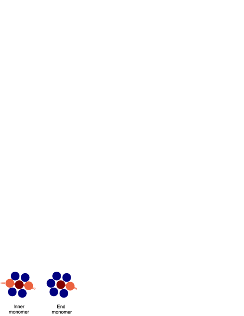
Figure 1: Sketch of the surroundings of a tagged (red) monomer of a linear polymer. Inner monomers are bonded to other two (light red) monomers. End monomers are bonded to a single one. The different connectivity alters the arrangement of the non-bonded (blue) nearest monomers ^{47, 48, 49, 50}.

RESULTS AND DISCUSSION

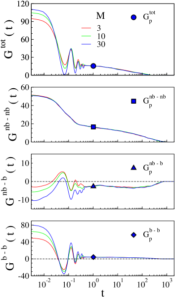
Figure 2: Stress correlation functions for the indicated chain lengths at $T=0.7$. The total stress correlation functions $G^{tot}(t)$, Eq.9, is plotted in the top panel. The other panels plot the different contributions to $G^{tot}(t)$ according to Eq. 9 and Eq. Finite frequency shear modulus. The symbols mark the values of $G^{tot}_{p}$ and $G^{l-m}_{p}$ according to Eq. 11 and Eq. 12

.

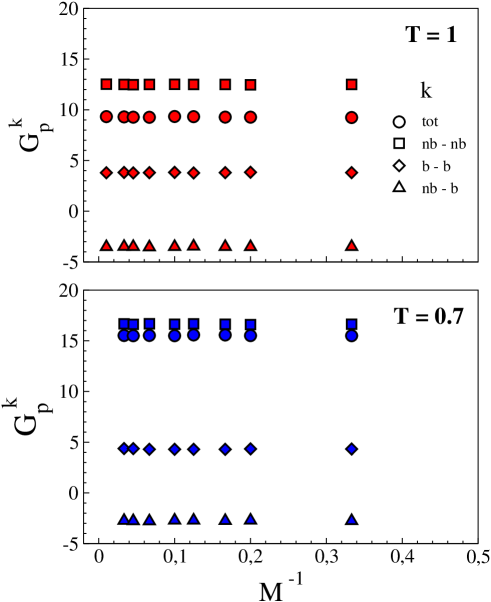
Figure 3: Chain length dependence of the finite frequency shear modulus $G^{tot}_{p}$, Eq.11 and the related contributions $G^{l-m}_{p}$ with $l,m\in\{b,nb\}$, Eq.12, at the indicated temperatures.

Finite frequency shear modulus

The off-diagonal $xy$ component of the stress tensor is defined by ¹⁰:

$$\sigma^{tot}_{xy}=\frac{1}{V}\left[\sum_{i=1}^{N}\left(mv_{x,i}v_{y,i}+\frac{1}{2}\sum_{j\neq i}r_{x,ij}F_{y,ij}\right)\right]$$ (3)

where $V=N/\rho$ is the volume of the system, $v_{\alpha,i}$ is the $\alpha$ component of the velocity of the $i$-th monomer, $r_{\alpha,ij}$ is the $\alpha$ component of the vector joining the $i$-th monomer with the $j$-th one and $F_{\alpha,ij}$ is the $\alpha$ component of the force between the $i$-th monomer and the $j$-th one.

Each monomer of the chain molecule is acted on by two distinct forces, ${\bf F}^{nb}$ and ${\bf F}^{b}$, due to the non-bonded and bonded potentials $U^{LJ}$ and $U^{b}$, respectively (see Sec.NUMERICAL METHODS and Fig.1 for details). In order to investigate the roles of the bonding interaction and the non-bonding LJ interaction separately, we recast $\sigma_{xy}^{tot}$ in Eq.3 as

$$\sigma_{xy}^{tot}=\sigma_{xy}^{b}+\sigma_{xy}^{nb}$$ (4)

with

$$\sigma_{xy}^{b} = \frac{1}{V}\left(\frac{1}{2}\sum_{i=1}^{N}\sum_{j\neq i}r_{x,ij}F_{y,ij}^{b}\right)$$ (5)

$$\sigma_{xy}^{nb} = \frac{1}{V}\left[\sum_{i=1}^{N}\left(mv_{x,i}v_{y,i}+\frac{1}{2}\sum_{j\neq i}r_{x,ij}F_{y,ij}^{nb}\right)\right]$$ (6)

The shear stress correlation function is defined by ³:

$$G_{xy}^{tot}(t)=\frac{V}{k_{B}T}\left\langle\sigma_{xy}^{tot}(t_{0})\sigma_{xy}^{tot}(t_{0}+t)\right\rangle$$ (7)

where the brackets $\langle\ldots\rangle$ denote the canonical average. The average value of $G_{xy}^{tot}(t)$, $G_{yz}^{tot}(t)$ and $G_{zx}^{tot}(t)$ will be denoted as $G^{tot}(t)$. Note that under equilibrium ^{3, 51}:

$$G^{tot}_{\infty}\equiv G^{tot}(0)=G_{\infty}$$ (8)

Splitting the total stress in bonded and non-bonded contributions as in Eq.4 recasts the stress correlation function as

$$G^{tot}(t)=\sum_{l,m\in\{b,nb\}}G^{l-m}(t)$$ (9)

with:

$$G^{l-m}(t)=\frac{V}{3k_{B}T}\Big{[}\left\langle\sigma_{xy}^{l}(t_{0})\sigma_{xy}^{m}(t_{0}+t)\right\rangle+$$ (10)

$$\left\langle\sigma_{yz}^{l}(t_{0})\sigma_{yz}^{m}(t_{0}+t)\right\rangle+\left\langle\sigma_{zx}^{l}(t_{0})\sigma_{zx}^{m}(t_{0}+t)\right\rangle\Big{]}$$

where $l,m\in\{b,nb\}$.

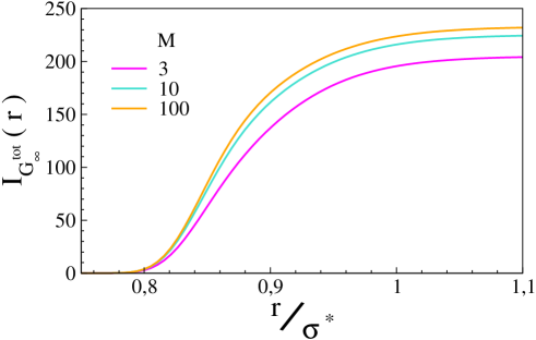
Figure 4: Plot of the integral $I_{G_{\infty}^{tot}}(r)=\int_{0}^{r}g(r^{\prime})\frac{d}{dr^{\prime}}\left[r^{\prime 4}\frac{dU(r^{\prime})}{dr^{\prime}}\right]dr^{\prime}$ for selected chain lengths and $T=1$. According to Eq. 13, $G_{\infty}^{tot}=\rho k_{B}T+\frac{2\pi}{15}\rho^{2}I_{G_{\infty}^{tot}}(\infty)$. The plot shows that $G_{\infty}^{tot}$ is largely due to the first neighbour shell located at $r\sim\sigma\sim\sigma^{*}$. For $M\geq 10$ the approximation given by Eq. 14 exceeds $G_{\infty}^{tot}$ by $\sim 5\%$.

Fig.2 shows the plots the total modulus $G^{tot}(t)$ and the distinct terms $G^{l-m}(t)$ of the right hand side of Eq.9 for the states at temperature $T=0.7$ and different chain lengths. At short times ($t\lesssim 0.5$) $G^{tot}(t)$ is characterized by oscillations with amplitude increasing with the chain length. Inspection of the bond-bond contribution $G^{b-b}(t)$ reveals that the oscillations are due to the bond length fluctuations, affecting in part the cross term $G^{nb-b}(t)$ too, whereas the non-bonded contribution $G^{nb-nb}(t)$ exhibits a smooth decrease at short times. For longer times ($t\gtrsim 0.5$) the oscillations of $G^{tot}(t)$ vanish and both the total modulus and the distinct bonded and non-bonded contributions approach a plateau-like region. The persistence of the elastic response is due to the cage effect , namely the trapping period of each monomer in the cage of the first neighbours which is terminated by the structural relaxation time $\tau_{\alpha}$ (for the present states $\tau_{\alpha}\sim 65$ ⁴⁸) ⁵². Beyond $\tau_{\alpha}$ $G^{tot}(t)$ relaxes according to the polymer viscoelasticity. We are not interested here in this long-time decay which has been addressed by other studies ¹³.

To begin with, we consider the intermediate plateau region and provide a convenient definition of the plateau height. From previous work it is known that for $t\lesssim 1$ the monomer explores the cage made by its first neighbors. At $t\sim 1$ early escape events become apparent by observing the monomer mean square displacement $\langle r^{2}(t)\rangle$ which exhibits a well-defined minimum of the logarithmic derivative quantity $\Delta(t)=\partial\langle r^{2}(t)\rangle/\partial\log t$ at $t=t^{*}\approx 1.02$ ^{53, 54, 55}. $t^{*}$ is a measure of the monomer trapping time and is independent of the physical state in the present polymer model ^{53, 54, 55}. We define the finite frequency shear modulus $G^{tot}_{p}$ and the related contributions according to Eq.9 as:

$$G^{tot}_{p} \equiv G^{tot}(t^{*})=G_{p}$$ (11)

$$G^{l-m}_{p} = G^{l-m}(t^{*}),\hskip 8.53581ptl,m\in\{b,nb\}$$ (12)

Fig.3 plots the plateau height and the related distinct contributions at two distinct temperatures. It is quite apparent that: i) they do no depend on the chain lenght and ii) $G^{nb-nb}_{p}$ is the main contribution to $G^{tot}_{p}$, especially at the lowest temperature, due to the virtual mutual cancellation of the other two contributions. Both findings fully comply with the conjecture formulated by Tobolsky for glassy polymers ²². Notably, the non-bonded contribution to the plateau modulus decreases with the temperature, whereas the other contributions are nearly constant due to the stiffness of the bonds and their subsequent quasi-harmonic character.

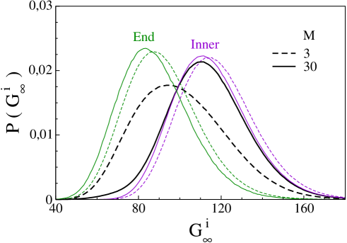
Figure 5: Distribution of the stiffness of the local environment surrounding the $i$-th monomer $G^{i}_{\infty}$ for two different chain lengths (black lines) at $T=1$. The overall distribution is a weighted sum of the two components related to the end monomers (green lines), and the inner monomers (violet lines) of each chains. Note that the two components are little dependent on the chain length, and the end monomers have lower average stiffness than the inner monomers due to the lower number of bonded interactions, see Fig.1.

Infinite frequency shear modulus

We now concentrate on the infinite-frequency shear modulus $G_{\infty}=G^{tot}_{\infty}$, Eq. 8, which is expressed as ^{3, 51}:

$$G_{\infty}^{tot} = \rho k_{B}T+\frac{2\pi}{15}\rho^{2}\int_{0}^{\infty}g(r)\frac{d}{dr}\left[r^{4}\frac{dU(r)}{dr}\right]dr$$ (13)

$$\simeq \rho k_{B}T+\frac{2\pi}{15}\rho^{2}\int_{0}^{\infty}r^{4}g(r)\frac{d^{2}U(r)}{dr^{2}}dr$$ (14)

where $g(r)$ and $U(r)$ are the radial distribution function and the interaction potential, respectively. The approximation given by Eq.14 follows by Fig.4 showing that the integral in Eq.13 is dominated by the region of the first shell, where $g(r)$ is maximum and the potential is close to the minimum at the investigated density and the chosen bond length. For $M\geq 10$ Eq. 14 exceeds $G_{\infty}^{tot}$ by $\sim 5\%$.

Eq.14 and Fig.4 emphasise that $G_{\infty}^{tot}$ is an average local stiffness due to the interactions between one central monomer and the closest neighbours. Thus, it is interesting to rewrite $G_{\infty}^{tot}$ as:

$$G_{\infty}^{tot}=\frac{1}{N}\sum_{i=1}^{N}G_{\infty}^{i}$$ (15)

$G_{\infty}^{i}$ has to be interpreted as a measure of the stiffness of the local environment surrounding the $i$-th monomer with radial distribution $g^{i}(r)$ :

$$G_{\infty}^{i}=\rho k_{B}T+\frac{2\pi}{15}\rho^{2}\int_{0}^{\infty}g^{i}(r)\frac{d}{dr}\left[r^{4}\frac{dU(r)}{dr}\right]dr$$ (16)

Fig.5 plots the overall distribution of the local stiffness for two different chain lengths and compares it to the same distribution restricted to the end and inner monomers. The end monomers are, on average, softer than the inner ones due to the lower connectivity, see Fig.1. The restricted distributions are little dependent on the chain length. Instead, the overall distribution depends on the chain length since changing the number of monomers per chain changes the relative weights of the end and the inner monomers.

Figure 6: Chain-length dependence of the infinite-frequency shear modulus $G^{tot}_{\infty}$ and the average local stiffnesses $\widetilde{G}_{\infty}^{X,A}$ with $X\in\{b,nb\},A\in\{E,I\}$ (see Eq.20) at the indicated temperatures.

The i-th monomer is surrounded by monomers which are either bonded or non-bonded to the former with radial distributions $g^{b,i}(r)$ and $g^{nb,i}(r)$, respectively. To investigate how the bonded and non-bonded monomers affect the local stiffness we separate the two contributions:

$$G_{\infty}^{i}=G_{\infty}^{b,i}+G_{\infty}^{nb,i}$$ (17)

with

$$G_{\infty}^{b,i} = \frac{2\pi}{15}\rho^{2}\int_{0}^{\infty}g^{b,i}(r)\frac{d}{dr}\left[r^{4}\frac{dU^{b}(r)}{dr}\right]dr$$ (18)

$$G_{\infty}^{nb,i} = \rho k_{B}T+\frac{2\pi}{15}\rho^{2}\int_{0}^{\infty}g^{nb,i}(r)\frac{d}{dr}\left[r^{4}\frac{dU^{LJ}(r)}{dr}\right]dr$$ (19)

The average values of the bonded contributions, $G_{\infty}^{b,i}$, over the end monomers and the inner monomers will be denoted as $\widetilde{G}_{\infty}^{b,E}$ and $\widetilde{G}_{\infty}^{b,I}$, respectively. The analogous averages of the non-bonded contributions, $G_{\infty}^{nb,i}$, will be denoted as $\widetilde{G}_{\infty}^{nb,E}$ and $\widetilde{G}_{\infty}^{nb,I}$. In practice, the infinite-frequency shear modulus is interpreted as an weighted sum of four different kinds of average local stiffnesses:

$$G_{\infty}^{tot}=\phi_{I}\Big{[}\widetilde{G}_{\infty}^{b,I}+\widetilde{G}_{\infty}^{nb,I}\Big{]}+\phi_{E}\Big{[}\widetilde{G}_{\infty}^{b,E}+\widetilde{G}_{\infty}^{nb,E}\Big{]}$$ (20)

where $\phi_{I}$ and $\phi_{E}$ are the relative weights of the inner and the end monomers, respectively:

$$\phi_{I} = \frac{M-2}{M}$$ (21)

$$\phi_{E} = \frac{2}{M}$$ (22)

Fig.6 shows the chain-length dependence of both $G_{\infty}^{tot}$ and the average local stiffnesses (see Eq.20). One notices that $G_{\infty}^{tot}$ increases with the chain length and the temperature, whereas $G_{p}^{tot}$ is independent of the chain length and decreases by increasing the temperature (see Fig.3). Furthermore, it is seen that $\widetilde{G}_{\infty}^{nb,I}$ and $\widetilde{G}_{\infty}^{nb,E}$ are weakly dependent on the chain length, whereas $\widetilde{G}_{\infty}^{b,I}$ and $\widetilde{G}_{\infty}^{b,E}$ are independent of that. In particular , it is seen that $\widetilde{G}_{\infty}^{b,I}\sim 2\widetilde{G}_{\infty}^{b,E}$ and $\widetilde{G}_{\infty}^{nb,E}>\widetilde{G}_{\infty}^{nb,I}$. This is due to the doubled bonded interactions of the inner monomers with respect to the end ones, and the corresponding decrease of the non bonded interactions with the first neighbours, see Fig.1. The residual chain-length dependence of the non-bonded terms of $\widetilde{G}_{\infty}$ in Fig.6 is readily explained by the fact that the average density around the end monomers is lower than the one around the inner monomers ³². Since the monomer density is kept constant and independent of the chain length, the increase of the chain length reduces the fraction of end monomers leading to the (slight) decrease of the density around all the other monomers and the subsequent (weak) softening of the non-bonded elasticity. Finally, we note that the temperature dependence of $G_{\infty}^{tot}$ has to be ascribed to the non-bonded interactions affecting $\widetilde{G}_{\infty}^{nb,E}$ and $\widetilde{G}_{\infty}^{nb,I}$. Fig.6 clarifies that the chain-length dependence of $G_{\infty}^{tot}$ is largely due to the change of the fractions of the inner and the end monomers, $\phi_{I}$ and $\phi_{E}$, rather than changes in the local stiffnesses.

CONCLUSIONS

An extended MD study of the short-time ”glassy” elasticity $G(t)$ of a polymer melt before the structural relaxation takes place has been carried out. Two characteristic regimes are noted. In the picosecond time scale, $G(t)$ approaches the affine, infinite-frequency modulus $G_{\infty}$ whereas, following the restoration of detailed mechanical equilibrium, $G(t)$ approaches the relaxed plateau $G_{p}$ which is terminated by the structural relaxation time $\tau_{\alpha}$.

$G_{\infty}$ depends on the chain length whereas $G_{p}$ is virtually independent of that. The dependence of $G_{\infty}$ on the chain length is ascribed to both the local character of $G_{\infty}$, mainly set by the stiffness of the interactions with the first neighbours, and the larger connectivity, via stiff bonds, of the inner monomers with respect to the end ones. The role of the connectivity is also exposed in the chain-length distribution of the local softness which follows by the range of different rigidity of the local environments which is fairly larger for inner monomers.

$G_{p}$ is not affected by the chain length and is largely set by the non-bonding interactions, thus confirming also for polymer melts above the glass transition the Tobolsky conjecture originally formulated for glassy polymers.

ACKNOWLEDGMENTS

A generous grant of computing time from IT Center, University of Pisa and Dell^® Italia is gratefully acknowledged.

References

- Doi and Edwards 1988 M. Doi and S. F. Edwards, The Theory of Polymer Dynamics (Clarendon Press, Oxford, 1988).
- Born and Huang 1962 M. Born and K. Huang, Dynamical Theory of Crystal Lattices (Oxford University Press, Oxford, 1962).
- Zwanzig and Mountain 1965 R. Zwanzig and R. Mountain, J. Chem. Phys. 43, 4464 (1965).
- Theodorou and Suter 1986a D. N. Theodorou and U. W. Suter, Macromolecules 19, 139 (1986a).
- Theodorou and Suter 1986b D. N. Theodorou and U. W. Suter, Macromolecules 19, 379 (1986b).
- Wallace 1972 D. C. Wallace, Thermodynamics of Crystals (Wiley, New York, 1972).
- Tsamados et al. 2009 M. Tsamados, A. Tanguy, C. Goldenberg, and J.-L. Barrat, Phys. Rev. E 80, 026112 (2009).
- Maloney and Lemaître 2006 C. E. Maloney and A. Lemaître, Phys. Rev. E 74, 016118 (2006).
- Yoshimoto et al. 2004 K. Yoshimoto, T. S. Jain, K. V. Workum, P. F. Nealey, and J. J. de Pablo, Phys. Rev. Lett. 93, 175501 (2004).
- Puosi and Leporini 2012 F. Puosi and D. Leporini, J. Chem. Phys. 136, 041104 (2012).
- Ladd et al. 1987 A. J. C. Ladd, W. E. Alley, and B. J. Alder, J. Stat. Physics 48, 1147 (1987).
- Yoshino and Mézard 2010 H. Yoshino and M. Mézard, Phys. Rev. Lett. 105, 015504 (2010).
- Likhtman et al. 2007 A. E. Likhtman, S. K. Sukumaran, and J. Ramirez, Macromolecules 40, 6748 (2007).
- Hsu 2002 S. L. Hsu, Vibrational Spectroscopy in Encyclopedia Of Polymer Science and Technology (Wiley, New York, 2002), vol. 8, pp. 311–381.
- Lunkenheimer and Loidl 2003 P. Lunkenheimer and A. Loidl, Phys. Rev. Lett. 91, 207601 (2003).
- Sibik et al. 2014 J. Sibik, S. R. Elliott, and J. A. Zeitler, J. Phys. Chem. Lett. 5, 1968 (2014).
- Krumbholz et al. 2011 N. Krumbholz, T. Hochrein, N. Vieweg, I. Radovanovic, I. Pupeza, M. Schubert, K. Kretschmer, and M. Koch, Polym. Eng. Sci. 51, 109 (2011).
- Nagai et al. 2004 N. Nagai, T. Imai, R. Fukasawa, K. Kato, and K. Yamauchi, Appl. Phys. Lett. 85, 4010 (2004).
- Rao and Pochan 2007 Y. Q. Rao and J. M. Pochan, Macromolecules 40, 290 (2007).
- Peiponen et al. 2015 K.-E. Peiponen, P. Bawuah, M. Chakraborty, M. Juuti, J. A. Zeitler, and J. Ketolainen, Int. J. Pharm., in press (2015).
- Sperling 2006 L. Sperling, Introduction to Physical Polymer Science (Wiley, New York, 2006).
- Tobolsky 1960 A. V. Tobolsky, Properties and Structure of Polymers (Wiley, New York, 1960).
- Hall 1989 C. Hall, Polymer materials: an introduction for technologists and scientists (Wiley, New York, 1989).
- Nielsen 1974 L. E. Nielsen, Mechanical Properties of Polymers and Composites, vol. 1 (M. Dekker, New York, 1974).
- Caulfield and Nissan 2007 D. F. Caulfield and A. H. Nissan, in Concise Encyclopedia of Composite Materials, edited by A. Mortensen (Elsevier, Amsterdam, 2007).
- Yannas and Luise 1982 I. V. Yannas and R. R. Luise, J. Macromol. Sci., Part B: Physics 21, 443 (1982).
- Theodorou and Suter 1985 D. N. Theodorou and U. W. Suter, Macromolecules 18, 1467 (1985).
- Lempesis et al. 2013 N. Lempesis, G. G. Vogiatzis, G. C. Boulougouris, L. C. van Breemen, M. Hütter, and D. N. Theodorou, Mol. Phys. 111, 3430 (2013).
- Hossain et al. 2010 D. Hossain, M. Tschopp, D. Ward, J. Bouvard, P. Wang, and M. Horstemeyer, Polymer 51, 6071 (2010).
- Schnell et al. 2011 B. Schnell, H. Meyer, C. Fond, J. Wittmer, and J. Baschnagel, Eur. Phys. J. E 34, 97 (2011).
- Ferry 1980 J. D. Ferry, Viscoelastic Properties of Polymers, III Ed. (Wiley, New York, 1980).
- Barbieri et al. 2004 A. Barbieri, D. Prevosto, M. Lucchesi, and D. Leporini, J. Phys.: Condens. Matter 16, 6609 (2004).
- Fetters et al. 2007 L. J. Fetters, D. J. Lohse, and R. H. Colby, in Physical Properties of Polymers Handbook, edited by J. E. Mark (Springer, Berlin, 2007), chap. 25, pp. 447–454.
- Strobl 2007 G. Strobl, The Physics of Polymers, III Ed. (Springer, Berlin, 2007).
- Inoue and Osaki 1996 T. Inoue and K. Osaki, Macromolecules 29, 1595 (1996).
- Baschnagel and Varnik 2005 J. Baschnagel and F. Varnik, J. Phys.: Condens. Matter 17, R851 (2005).
- Grest and Kremer 1986 G. S. Grest and K. Kremer, Phys. Rev. A 33, 3628 (1986).
- Plimpton 1995 S. Plimpton, J. Comput. Phys. 117, 1 (1995).
- Alessi et al. 2001 L. Alessi, L. Andreozzi, M. Faetti, and D. Leporini, J.Chem.Phys. 114, 3631 (2001).
- Leporini 1994 D. Leporini, Phys. Rev. A 49, 992 (1994).
- Andreozzi et al. 1999 L. Andreozzi, M. Faetti, M. Giordano, and D. Leporini, J.Phys.:Condens. Matter 11, A131 (1999).
- Prevosto et al. 2004 D. Prevosto, S. Capaccioli, M. Lucchesi, D. Leporini, and P. Rolla, J. Phys.: Condens. Matter 16, 6597 (2004).
- Kremer and Grest 1990 K. Kremer and G. S. Grest, J. Chem. Phys. 92, 5057 (1990).
- Kröger 2004 M. Kröger, Phys. Rep. 390, 453 (2004).
- Paul and Smith 2004 W. Paul and G. D. Smith, Rep. Prog. Phys. 67, 1117 (2004).
- Luo and Sommer 2009 C. Luo and J.-U. Sommer, Comp. Phys. Comm. 180, 1382 (2009).
- Larini et al. 2005 L. Larini, A. Barbieri, D. Prevosto, P. A. Rolla, and D. Leporini, J. Phys.: Condens. Matter 17, L199 (2005).
- Bernini et al. 2015a S. Bernini, F. Puosi, and D. Leporini, J. Non-Cryst. Solids 407, 29 (2015a).
- Bernini et al. 2013 S. Bernini, F. Puosi, M. Barucco, and D. Leporini, J. Chem. Phys. 139, 184501 (2013).
- Bernini et al. 2015b S. Bernini, F. Puosi, and D. Leporini, J. Chem. Phys. 142, 124504 (2015b).
- Boon and Yip 1980 J. P. Boon and S. Yip, Molecular Hydrodynamics (Dover Publications, New York, 1980).
- Götze 2008 W. Götze, Complex Dynamics of Glass-Forming Liquids: A Mode-Coupling Theory (Oxford University Press, Oxford, 2008).
- Puosi et al. 2013 F. Puosi, C. D. Michele, and D. Leporini, J. Chem. Phys. 138, 12A532 (2013).
- Ottochian et al. 2009 A. Ottochian, C. De Michele, and D. Leporini, J. Chem. Phys. 131, 224517 (2009).
- Larini et al. 2008 L. Larini, A. Ottochian, C. De Michele, and D. Leporini, Nature Physics 4, 42 (2008).