Queueing Stability and CSI Probing of a TDD Wireless Network with Interference Alignment

Abstract

This paper characterizes the performance of interference alignment (IA) technique taking into account the dynamic traffic pattern and the probing/feedback cost. We consider a time-division duplex (TDD) system where transmitters acquire their channel state information (CSI) by decoding the pilot sequences sent by the receivers. Since global CSI knowledge is required for IA, the transmitters have also to exchange their estimated CSIs over a backhaul of limited capacity (i.e. imperfect case). Under this setting, we characterize in this paper the stability region of the system under both the imperfect and perfect (i.e. unlimited backhaul) cases, then we examine the gap between these two resulting regions. Further, under each case, we provide a centralized probing algorithm (policy) that achieves the max stability region. These stability regions and scheduling policies are given for the symmetric system where all the path loss coefficients are equal to each other, as well as for the general system. For the symmetric system, we compare the stability region of IA with the one achieved by a time division multiple access (TDMA) system where each transmitter applies a simple singular value decomposition technique (SVD). We then propose a scheduling policy that consists in switching between these two techniques, leading the system, under some conditions, to achieve a bigger stability region. Under the general system, the adopted scheduling policy is of a high computational complexity for moderate number of pairs, consequently we propose an approximate policy that has a reduced complexity but that achieves only a fraction of the system stability region. A characterization of this fraction is provided.

I Introduction

One of the key issues in wireless communication systems is the interference that is caused by a large number of users communicating on the same channel, resulting into severe performance degradations unless treated properly. In this regard, interference alignment (IA) was introduced in [2] as an efficient interference management technique and is shown to result in higher throughputs compared to conventional interference-agnostic methods. Indeed, IA is a linear precoding technique that attempts to align interfering signals in time, frequency, or space. In multiple-input multiple-output (MIMO) networks, IA utilizes the spatial dimension offered by multiple antennas for alignment. By aligning interference at all receivers (users), IA reduces the dimension of interference, allowing users to suppress interference via linear techniques and decode their desired signals interference free. However, the implementation of IA in existing systems faces some challenges. A major disadvantage of the above IA scheme lies in the fact that the global channel state information (CSI) must be available at each transmitter, which weakens its application in practical systems, because CSI, especially interference CSI, is difficult to obtain at the transmitters.

In scenarios where the receivers quantize and send the CSI back to the transmitters, the IA scheme is explored over frequency selective channels for single-antenna users in [3] and for multiple-antenna users in [4]. Both references provide degree-of-freedom (DoF)-achieving quantization schemes and establish the required scaling of the number of feedback bits. For alignment using spatial dimensions, [5] provides the scaling of feedback bits to achieve IA in MIMO interference channel (IC). For the broadcast channel, the scaling of the feedback bits was characterized in [6]. In [7], quantization of the precoding matrix using random vector quantization (RVQ) codebooks is investigated, which provides insights on the asymptotic optimality of RVQ. To overcome the problem of scaling codebook size, and relax the reliance on frequency selectivity for quantization, [8] proposed an analog feedback strategy for constant MIMO interference channels. From another point of view, [9] provides an analysis of the effect of imperfect CSI on the mutual information of the interference alignment scheme. On the other side, for time-division duplex (TDD) systems, every transmitter can estimate its downlink channels from the uplink transmission phase thanks to reciprocity. However, for the IA scheme, this local knowledge is not sufficient, and the transmitters need to share their channel estimates that can be carried out through backhaul links between transmitters. These links generally have a limited capacity, which should be exploited efficiently. For instance, in [10] a compression scheme for the cloud radio access networks is proposed. In [11], the Grassmannian Manifold quantization technique was adopted to reduce the information exchange over the backhaul. The above works on IA and limited feedback do not take into account the dynamic traffic processes of the users, meaning that they assume users with infinite back-logged data.

It is of great interest to investigate the impact of MIMO in the higher layers [12], more specifically in the media access control (MAC) layer. The cross-layer design goal here is the achievement of the entire stability region of the system. In broad terms, the stability region of a network is the set of arrival rate vectors such that the entire network load can be served by some service policy without an infinite blow up of any queue. The special scheduling policy achieving the entire stability region, called the stability-optimal policy (or simply optimal policy), is hereby of particular interest. The concept of stability-optimal operation comes originally from the control and automation theory [13, 14, 15, 16]. It was applied to the wireless communication systems first in [17], and the view was extended by some bounds in [18]. Since then, this concept has been investigated in the wireless framework under various traffic and network scenarios. For instance, in [19], the authors have presented a precoding strategy that achieves the system stability region, under the assumptions of perfect CSI and use of Gaussian codebooks. This strategy is based on Lyapunov drift minimization given the queue lengths and channel states every timeslot. Authors in [20] have considered the broadcast channel (BC) and proposed a technique based on zero forcing (ZF) precoding, with a heuristic user scheduling scheme that selects users whose channel states are nearly orthogonal vectors and illustrate the stability region this policy achieves via simulations. In [21], it has been noticed that the policy resulting from the minimization of the drift of a quadratic Lyapunov function is to solve a weighted sum rate maximization problem (with weights being the queue lengths) each timeslot and they propose an iterative water-filling algorithm for this purpose. In addition, authors in [22] propose to use the delays of the packets in the head of each queue along with the queue lengths as weights. All these works assume accurate CSI available at the transmitter. In the case of delayed channel state information and channels having a correlation in time, authors in [23] compare the stability and delay performance of opportunistic beamforming and space time coding, while in [24] they propose a user scheduling and precoding algorithm. Further, in [25], the authors studied the impact of channel state quantization on the stability of a system using ZF precoding under a centralized scheme where the transmitter selects the users to be scheduled based only on the queue lengths. However, in these works, the fact that radio resources i.e. time and/or spectrum are needed to acquire channel state information is not accounted for. For the case where the CSI acquisition process consumes a fraction of the timeslot, the authors in [26] have explored the resulting trade-off between acquiring CSI and exploiting channel diversity to the various receiver. In addition, taking into account the probing cost, the authors in [27] have examined three different scheduling policies (centralized, decentralized and mixed policies) for MISO wireless downlink systems under ZF precoding technique. It is worth noting that all the aforementioned works consider networks with a relatively simple physical layer (e.g. on-off channel, ZF, …).

In this paper, we have a system with a more complicated physical layer. Specifically, we consider a Multipoint-to-Multipoint network where multiple transmitter-receiver pairs operate in TDD mode and apply the IA technique under backhaul links of limited capacity. Each transmitter acquires its local CSI from its corresponding user by exploiting the channel reciprocity. Indeed, there are two ways to perform this acquisition (probing): (i) users estimate their channels and then feed the CSI back to their corresponding transmitters in a time division multiple access (TDMA) manner, and (ii) users send training sequences in the uplink so that the transmitters can estimate the channels. The latter scheme, which we adopt in our system, uses (pre-assigned) orthogonal sequences among the users, so the length of each one of these sequences should be proportional to the number of active users in the system; orthogonal sequences are produced e.g. by Walsh-Hadamard on pseudonoise sequences. It means that after acquiring the CSI of, for example, $L$ users, the throughput is multiplied by $1-L\theta$, where $\theta$ is the fraction of time that takes the CSI acquisition of one user [26]. Thus, it can be seen that the more the number of active pairs $L$ is large, the more the acquisition process consumes a larger fraction of time and hence leaves a smaller fraction for transmission. Thus, it is important to focus on the tradeoff between having a large number of active transmitter-receiver pairs (so having a high probing cost but many pairs can communicate simultaneously) and having much time of the slot dedicated to data transmission (which means getting a low probing cost but few pairs can communicate simultaneously) [27]. Therefore, under this scheme, it can happen that only a subset of transmitter-receiver pairs is active (scheduled) at each timeslot.

In order to choose the subset of active pairs at each timeslot, three approaches can be used [27]: (i) the centralized scheme (policy), where the decision of which pairs will be scheduled is made at the transmitters side and based only on the statistics of the channels of the users and the state of their queue lengths at each slot [25], (ii) the decentralized scheme, meaning that the users decide which subset of them should actually train, and consequently this subset with its corresponding subset of transmitters will be active for transmission, and (iii) the mixed policy, which corresponds to combine the centralized and decentralized policies. Note that the centralized approach is used in current standards (e.g. Long Term Evolution (LTE) [28]), where the base station explicitly requests some users for their CSI.

In this paper, we adopt the first approach, that is the centralized policy. Specifically, for the MIMO system model described earlier, in which we use IA as an interference management technique, we consider that there is a central scheduler (CS) that has a full knowledge of the queue lengths at each timeslot and the statistics of the channels. Based on this information, this CS schedules the subset of pairs at each timeslot. In broad terms, using the centralized policy, we examine in this work the stability performances of a MIMO system under TDD mode with limited backhaul capacity, where we apply IA as an effective way to reduce the interference and where the CSI probing cost is accounted for.

It is known that with IA technique the backhaul is flooded due to the CSI exchange process among the active transmitters. In some scenarios, it may be beneficial not to occupy the backhaul with this huge amount of signaling but instead exploited it more efficiently. For instance, if the backhaul is wireless, the CSI exchange process consumes a part of the total reserved bandwidth, which can be instead used in the transmission process. Hence, it is of high interest to study the system under an interference management technique for which no CSI exchange over the backhaul is required. For this purpose, we investigate the system performance under TDMA as a channel access method, meaning that there is only one active pair at a given timeslot and thus no backhaul usage occurs, and using singular value decomposition (SVD) as a precoding technique. The choice of SVD can be justified by the fact that it provides the best performances for point-to-point MIMO systems [29]. One may wonder which one between TDMA-SVD and IA outperforms the other in terms of stability. We will provide an answer to this question by comparing the system stability performances under these two techniques.

The rest of this paper is organized as follows. Section II presents the system model and the interaction between physical layer and queueing performance. The average rate expressions under the adopted system are derived in Section III. In Section IV, we present a deep stability analysis for the symmetric system where all the path loss coefficients are equal to each other. Specifically, for this system, we provide a precise characterization of the stability region and we propose an optimal scheduling decision to achieve this region in both the perfect and imperfect cases. Further, we examine the gap between these two resulting stability regions, namely the region under the imperfect case and the one under the perfect case. Furthermore, for this same system, we compare the stability region of IA with the one achieved by TDMA-SVD, then, using this comparison, we provide a way to select one of these two techniques. In addition, we characterize the resulting stability region when the considered system switches between these two techniques. At the end of this section, we investigate the impact of the number of bits and the number of pairs on the system stability region. In Section V, we investigate the stability performances for the general case, namely where the path loss coefficients are not necessarily equal to each other, by characterizing the corresponding stability region and providing an optimal scheduling policy, under both the imperfect and perfect cases. Then, since the scheduling policy for this system is of high computational complexity, we propose an approximate policy that has a reduced complexity but that achieves only a fraction of the system stability region. After that, a characterization of the achievable fraction is provided. At the end of this section, we investigate the gap between the stability region under the imperfect case and the one under the perfect case. Section VI is dedicated to numerical results. Finally, Section VII concludes the paper.

Notation: Boldface uppercase symbols (i.e., ${\bf A}$) represent matrices and lowercases (i.e., ${\bf a}$) are used for vectors, unless stated otherwise. The symbol ${\bf I}_{N}$ denotes the identity matrix of size $N$. The operator $\otimes$ is the Kronecker product. The notation $|\cdot|$ is used to indicate the absolute value for scalars and the cardinality for sets (or subsets). In addition, $||\cdot||_{1}$ and $||\cdot||$ are used for the norms of first and second degree, respectively. The notation $\mathbf{1}$ is used for the all-ones vector. Finally, superscripts $T$ and $H$ over a matrix or vector denote its transpose and conjugate transpose, respectively.

II System Model

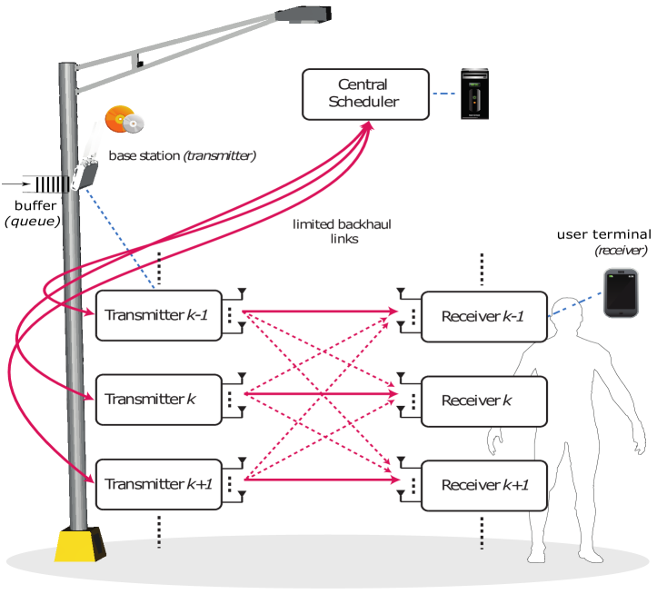
Figure 1: A sketch of $N$-user MIMO interference network with limited backhaul.

We consider the MIMO interference channel with $N$ transmitter-receiver pairs shown in Fig. 1. For simplicity of exposition, we consider a homogeneous network where all transmitters are equipped with $N_{\text{t}}$ antennas and all receivers (users) with $N_{\text{r}}$ antennas. We assume that time is slotted. As we will see later on, only a subset $\mathcal{L}(t)$, of cardinality $L(t)$, of pairs is active at each timeslot, with $L(t)\leq N$. While each transmitter communicates with its intended receiver, it also creates interference to other $L(t)-1$ unintended receivers. Transmitter $k$ has $d_{k}\leq\min\left(N_{\text{t}},N_{\text{r}}\right)$ independent data streams to transmit to its intended user $k$.

Given this channel model, the received signal at active user $k$ ($\in\mathcal{L}(t)$) can be expressed as

$$\mathbf{y}_{k}=\sum\limits_{i\in\mathcal{L}(t)}\sqrt{\frac{\zeta_{ki}P}{d_{i}}}\mathbf{H}_{ki}\sum\limits_{j=1}^{d_{i}}\mathbf{v}_{i}^{(j)}x_{i}^{(j)}+\mathbf{z}_{k},$$ (1)

where $\mathbf{y}_{k}$ is the $N_{r}\times 1$ received signal vector, $\mathbf{z}_{k}$ is the additive white complex Gaussian noise with zero mean and covariance matrix $\sigma^{2}\mathbf{I}_{N_{\text{r}}}$, $\mathbf{H}_{ki}$ is the $N_{\text{r}}\times N_{\text{t}}$ channel matrix between transmitter $i$ and receiver $k$ with independent and identically distributed (i.i.d.) zero mean and unit variance complex Gaussian entries, $\zeta_{ki}$ represents the path loss of channel $\mathbf{H}_{ki}$, $P$ is the total power at each transmitting node, which is equally allocated among its data streams, $x_{i}^{(j)}$ represents the $j$-th data stream from transmitter $i$, and $\mathbf{v}_{i}^{(j)}$ is the corresponding $N_{\text{t}}\times 1$ precoding vector of unit norm. For the rest of the paper, we denote by $\alpha_{ki}$ the fraction $\frac{\zeta_{ki}P}{d_{i}}$.

II-A Interference Alignment Technique

IA is an efficient linear precoding technique that often achieves the full DoF supported by MIMO interference channels. In cases where the full DoF cannot be guaranteed, IA has been shown to provide significant gains in high signal-to-noise ratio (SNR) sum-rate. To investigate IA in our model, we start by examining the effective channels created after precoding and combining. For tractability, we restrict ourselves to a per-stream zero-forcing receiver. Recall that in the high (but finite) SNR regime, in which IA is most useful, gains from more involved receiver designs are limited [30]. In such a system, receiver $k$ uses the $N_{\text{r}}\times 1$ combiner vector $\mathbf{u}_{k}^{m}$ of unit norm to detect its $m$-th stream, such as

$$\hat{x}_{k}^{(m)} =\left(\mathbf{u}_{k}^{(m)}\right)^{\!H}\mathbf{y}_{k}$$

$$=\overbrace{\sqrt{\alpha}_{kk}\left(\mathbf{u}_{k}^{(m)}\right)^{\!H}\mathbf{H}_{kk}\mathbf{v}_{k}^{(m)}x_{k}^{(m)}}^{\text{desired signal}}+\overbrace{\sqrt{\alpha}_{kk}\sum_{j=1,j\neq m}^{d_{k}}\left(\mathbf{u}_{k}^{(m)}\right)^{\!H}\mathbf{H}_{kk}\mathbf{v}_{k}^{(j)}x_{k}^{(j)}}^{\text{inter-stream interference (ISI)}}$$

$$\qquad{}+\overbrace{\sum\limits_{\begin{subarray}{c}i\in\mathcal{L}(t),i\neq k\end{subarray}}\sqrt{\alpha}_{ki}\sum\limits_{j=1}^{d_{i}}\left(\mathbf{u}_{k}^{(m)}\right)^{\!H}\mathbf{H}_{ki}\mathbf{v}_{i}^{(j)}x_{i}^{(j)}}^{\text{inter-user interference (IUI)}}+\overbrace{\left(\mathbf{u}_{k}^{(m)}\right)^{\!H}\mathbf{z}_{k}}^{\text{noise}},$$ (2)

where the first term at the right-hand-side of this expression is the desired signal, the second one is the inter-stream interference (ISI) caused by the same transmitter, and the third one is the inter-user interference (IUI) resulting from the other transmitters. In order to mitigate these interferences and improve the system performances, IA is performed accordingly, that is designing the set of combiner and precoder vectors such that

$$\left(\mathbf{u}_{k}^{(m)}\right)^{\!H}\mathbf{H}_{ki}\mathbf{v}_{i}^{(j)}=0, \forall(i,j)\neq(k,m),\text{with}\,i,k\in\mathcal{L}(t).$$ (3)

Note that the above conditions are those of a perfect interference alignment. In other words, suppose that all the transmitting nodes have perfect global CSI and each receiver obtains a perfect version of its corresponding combiner vector, ISI and IUI can be suppressed completely. However, obtaining the perfect global CSI at the transmitters is not always practical due to the fact that backhaul links, which connect transmitters to each other, are of limited capacity. The CSI sharing mechanism is detailed in the next subsection.

Finally, some assumptions and remarks are in order. First, in our study, we assume that each active receiver obtains a perfect version of its corresponding combiner vector. The cost of this latter process is not considered in our analysis. In addition, it is worth noting that due to the limitation of spatial degree of freedom, the values of $d_{k}$ must fulfill the feasibility conditions of IA [31]. In what follows, we suppose IA is feasible by selecting the data steams numbers $d_{k}$ carefully. Further, we recall that the total transmit power is split equally among the transmitters, and then each of which equally allocates its power among its data streams; it means that we do not perform power control for our system. This is done to further simplify the transmission scheme that relies on IA technique, which does not lack complexity.

II-B CSIT Sharing Over Limited Capacity Backhaul Links

The process of CSI sharing is restricted to the scheduled pairs (represented by subset $\mathcal{L}(t)$). Thus, here, even if we did not mention it, when we write “transmitter” (resp., “user”) we mean “active transmitter” (resp., “active user”). Three different scenarios regarding the CSI sharing problem can be considered:

1. Each transmitter receives all the required CSI and independently computes the IA vectors,

2. The IA processing node is a separate central node that computes and distributes the IA vectors to other transmitters,

3. One transmitter acts as the IA processing node.

For the last two scenarios, one node performs the computations and then distributes the IA vectors among transmitters. So, since the backhaul is limited in capacity, in addition to the quantization required for the CSI sharing process, another quantization is needed to distribute the IA vectors over the backhaul. This is not the case for the first scenario where only the first quantization process is needed. Thus, for simplicity of exposition and calculation, we focus on the first scenario, which we detail in the following.

As alluded earlier, global CSI is required at each transmitting node in order to design the IA vectors that satisfy (3). As shown in Fig. 1, we suppose that all the transmitters are connected to a CS via their limited backhaul links, meaning that this CS serves as a way for connecting the transmitters to each other; as we will see later on, this scheduler decides which pairs to schedule at each timeslot. We assume a TDD transmission strategy, which enables the transmitters to estimate their channels toward different users by exploiting the reciprocity of the wireless channel. We consider throughout this paper that there are no errors in the channel estimation. Under the adopted strategy, the users send their training sequences in the uplink phase, allowing each transmitter to estimate (perfectly) its local CSI, meaning that the $i$-th transmitter estimates perfectly the channels $\mathbf{H}_{ki}$, $k,i\in\mathcal{L}(t)$. However, the local CSI, excluding the direct links (since they do not enter in computing the IA vectors), of other transmitters are obtained via backhaul links of limited capacity. In such limited backhaul conditions, a codebook-based quantization technique needs to be adopted to reduce the huge amount of information exchange used for CSI sharing, which we detail as follows. Let $\mathbf{h}_{ki}$ denote the vectorization of the channel matrix $\mathbf{H}_{ki}$. Then, for all $i\neq k$, transmitter $i$ selects the index $n_{o}$ that corresponds to the optimal codeword in a predetermined codebook $\mathcal{CB}=\left[\mathbf{\hat{h}}_{ki}^{(1)},...,\mathbf{\hat{h}}_{ki}^{(2^{B})}\right]$ according to

$$n_{o}=\operatorname*{arg\,max}_{1\leq n\leq 2^{B}}\left\{\left|\left(\mathbf{\tilde{h}}_{ki}\right)^{\!H}\,\mathbf{\hat{h}}_{ki}^{(n)}\right|^{2}\right\},$$ (4)

in which $B$ is the number of bits used to quantize $\mathbf{H}_{ki}$ and $\mathbf{\tilde{h}}_{ki}=\frac{\mathbf{h}_{ki}}{\left\|\mathbf{h}_{ki}\right\|}$ is the channel direction vector. After quantizing all the matrices of its local CSI, we assume that transmitter $i$ sends the corresponding optimal indexes to all other active transmitters, which share the same codebook, allowing these transmitters to reconstruct the quantized local knowledge of transmitter $i$. Let us now define the quantization error as $e_{ki}=1-\frac{\left|\mathbf{\hat{h}}_{ki}^{H}\mathbf{h}_{ki}\right|^{2}}{\left\|\mathbf{h}_{ki}\right\|^{2}}$ and adopt the same model in [6, 25] that relies on the theory of quantization cell approximation. The cumulative distribution function (CDF) of $e_{ki}$ is then given by

$$\mathbb{P}\left\{e_{ki}\leq\varepsilon\right\}=\begin{dcases}2^{B}\varepsilon^{Q},&\qquad{}0\leq\varepsilon\leq 2^{-\frac{B}{Q}}\\ 1,&\qquad{}\,\varepsilon>2^{-\frac{B}{Q}}\end{dcases}$$ (5)

where $Q=N_{\mathrm{t}}N_{\mathrm{r}}-1$.

II-C Rate Model and Impact of Training

Before proceeding with the description, we define the perfect case as the case where the backhaul has an infinite capacity, which leads to a perfect global CSI knowledge at the transmitters; so no quantization is needed. Further, we call imperfect case the model described previously, where a quantization is performed over the backhaul of limited capacity.

For the perfect case, the IA constraints null the ISI and the IUI, and no residual interference exists. For the imperfect case, as explained in the previous subsection, each transmitter designs its IA vectors based on a perfect version of its local CSI and an imperfect (quantized) version of the local CSI of other transmitters. For this reason, in this case, the IA technique is able to completely cancel the ISI but not the IUI. Thus, under such observations, the SINR/SNR for stream $m$ at active receiver $k$ can be written as

$$\gamma_{k}^{(m)}=\begin{dcases}\,\,\frac{\alpha_{kk}\left|\left(\mathbf{\hat{u}}_{k}^{(m)}\right)^{\!H}\mathbf{H}_{kk}\mathbf{\hat{v}}_{k}^{(m)}\right|^{2}}{\sigma^{2}+\sum\limits_{\begin{subarray}{c}i\in\mathcal{L}(t),i\neq k\end{subarray}}\alpha_{ki}\sum\limits_{j=1}^{d_{i}}\left|\left(\mathbf{\hat{u}}_{k}^{(m)}\right)^{\!H}\mathbf{H}_{ki}\mathbf{\hat{v}}_{i}^{(j)}\right|^{2}},&\qquad{}\text{imperfect case}\\ \,\,\frac{\alpha_{kk}\left|\left(\mathbf{u}_{k}^{(m)}\right)^{\!H}\mathbf{H}_{kk}\mathbf{v}_{k}^{(m)}\right|^{2}}{\sigma^{2}},&\qquad{}\text{perfect case}\end{dcases}$$ (6)

where $\mathbf{\hat{v}}_{k}^{(m)}$ and $\mathbf{\hat{u}}_{k}^{(m)}$ are designed under the limited backhaul case, that is to say using an imperfect global CSI due to the quantization process over the backhaul, whereas $\mathbf{v}_{k}^{(m)}$ and $\mathbf{u}_{k}^{(m)}$ are designed under the unlimited backhaul case, i.e. using a perfect global CSI. As alluded earlier, only a subset $\mathcal{L}(t)$ (we recall that $\left|\mathcal{L}(t)\right|=L(t)$) of pairs is scheduled at a time. For notational convenience, we will use signal-to-interference-plus-noise ratio (SINR) as a general notation to denote SNR for the perfect case and SINR for the imperfect case, unless stated otherwise.

We now explain some useful points that are adopted in the rate model. At a given timeslot, a rate of $R$ bits is assigned to stream $m$ of user $k$ if $\gamma_{k}^{(m)}$, i.e. the corresponding SINR, is higher than or equal to a given threshold, which we denote by $\tau$; otherwise, the assigned rate is $0$. Let us denote by $\tilde{R}_{k}(t)$ the assigned rate (in units of bits/slot) for user $k$ at timeslot $t$, thus $\tilde{R}_{k}(t)$ is the sum of the assigned rates for all the streams of user $k$ at $t$. For this model, channel acquisition cost is not negligible and should be considered. As mentioned earlier, we consider a system under TDD mode where users send training sequences in the uplink so that the transmitters can estimate their channels; this is a promising approach, especially for systems with large antenna arrays at the transmitters, due to the fact that the feedback overhead does not scale with the number of antennas. This scheme uses orthogonal sequences among the users, so their lengths are proportional to the number of active users in the system. We assume that acquiring the CSI of one user takes fraction $\theta$ of the slot. Thus, since we have $L(t)$ active users, the actual rate for transmission to active user $k$ at timeslot $t$ is $(1-L(t)\theta)\tilde{R}_{k}(t)$. Let us define $B_{k}(t)=(1-L(t)\theta)\tilde{R}_{k}(t)$. Note that $B_{k}(t)$ is equal to $0$ if pair $k$ is not active at time $t$.

Under this setting, the average rate for active user $k$ can be written in function of the transmission success probability conditioned on the subset of active pairs as

$$\mathbb{E}\left\{B_{k}(t)\mid\mathcal{L}(t)\right\}=(1-L(t)\theta)\sum_{m=1}^{d_{k}}R\,\mathbb{P}\left\{\gamma_{k}^{(m)}\geq\tau\mid\mathcal{L}(t)\right\}.$$ (7)

It can be noticed that the feedback overhead ($1-L(t)\theta$) scales with the number of active pairs, meaning that when $L(t)$ is large there will be little time left to transmit in the timeslot before the channels change again. Here, it is clear that the fraction $L(t)\theta$ should be lower than $1$. Since the maximum number of pairs $N$ is such that $N\geq L(t)$, we should also have $N\theta<1$. In practice, the fraction of the timeslot dedicated for CSI acquisition is less than $\frac{1}{2}$, i.e. at least half of the timeslot is reserved for data transmission.

II-D Queue Dynamics, Stability and Scheduling Policy

For each user, we assume that the incoming data is stored in a respective queue (buffer) until transmission, and we denote by $\mathbf{q}(t)=\left[q_{1}(t),...,q_{N}(t)\right]$ the queue length vector. We designate by $\mathbf{A}(t)=\left[A_{1}(t),...,A_{N}(t)\right]$ the vector of number of bits arriving in the buffers in timeslot $t$, which is an i.i.d. in time process, independent across users and with $A_{k}(t)<A_{\text{max}}$. The mean arrival rate (in units of bits/slot) for user $k$ is denoted by $a_{k}=\mathbb{E}[A_{k}(t)]$. We recall that a user will get $B_{k}(t)$ served bits per slot if it gets scheduled and zero otherwise. Note that $B_{k}(t)$ is finite because $R$ is finite, so we can define a finite positive constant $B_{\text{max}}$ such that $B_{k}(t)<B_{\text{max}}$, for $k=1,\ldots,N$.

At each timeslot, the CS selects the pairs to schedule based on the queue lengths and average rates (per user) in the system. To this end, we suppose that (i) this scheduler has a full knowledge of average rate values under different combinations of choosing active pairs, which can be provided offline since an average rate is time-independent, (ii) at each timeslot, each transmitter sends its queue length to the CS so that it can obtain all the queue dynamics of the system, and (iii) the cost of providing such knowledge to the scheduler will not be taken into account in our analysis. After selecting the set of pairs to be scheduled (represented by $\mathcal{L}(t)$), the CS broadcasts this information so that the selected transmitter-user pairs activate themselves, and then the active users send their pilots in the uplink so that the (active) transmitters can estimate the CSI. It is worth noting that, as alluded previously, if we select a large number of pairs ($L(t)$) for transmission, many pairs can communicate (i.e. this will leave a small fraction of time for transmission) but a high CSI acquisition cost is needed. On the other hand, a small $L(t)$ requires a low acquisition cost, but, at the same time, it allows a few number of simultaneous transmissions. The decision of selecting active pairs is referred simply as the scheduling policy. At the $t$-th slot, this policy can be represented by an indicator vector $\mathbf{s}(t)\in\mathcal{S}\coloneqq\left\{0,1\right\}^{N}$, where the $k$-th component of $\mathbf{s}(t)$, denoted by $s_{k}(t)$, is equal to $1$ if the $k$-th queue (pair) is scheduled or otherwise equal to $0$. It can be seen that the cardinality of set $\mathcal{S}$ is equal to $\left|\mathcal{S}\right|=2^{N}$. Remark that, in terms of notation, $\mathbf{s}(t)$ and $\mathcal{L}(t)$ are used to represent the same thing, that is the scheduled pairs at timeslot $t$, but they illustrate it differently. Specifically, using $\mathbf{s}(t)$ the active pairs correspond to the non-zero coordinates (equal to $1$), whereas $\mathcal{L}(t)$ contains the indexes (positions) of these pairs. Let $\bm{\mathcal{L}}$ be the set of all possible subsets $\mathcal{L}(t)$.

Now, using the definition of $B_{k}(t)$, which was provided earlier, the queueing dynamics (i.e. how the queue lengths evolve over time) can be described by the following

$$q_{k}(t+1)=\max\left\{q_{k}(t)-B_{k}(t),0\right\}+A_{k}(t),\qquad\,\,\forall k\in\{1,\ldots,N\},\forall t\in\{0,1,\ldots\},$$ (8)

where we note that $B_{k}(t)$ depends on the scheduling policy.

In this work, the focus will be mainly on the stability of the system. Formally, its definition is as follows.

Definition 1 (Strong Stability).

The condition for strong stability of the system can be expressed as the following

$$\underset{T\rightarrow\infty}{\lim\sup}\frac{1}{T}\sum\limits_{t=0}^{T-1}\mathbb{E}\left\{q_{k}(t)\right\}<\infty,\forall k\in\{1,...,N\}.$$ (9)

From this definition, stability implies that the mean queue length of every queue in the system is finite, further implying finite delays in single hop systems. Note that in the remainder of the manuscript “stable” will imply “strongly stable” unless stated otherwise. This definition leads us to the concept of stability region.

Definition 2 (Stability Region).

The stability region can be defined as the set of mean arrival rate vectors for which all the queues are strongly stable. Furthermore, a scheduling policy (algorithm) that achieves this region is called throughput optimal.

For the rest of the paper, when describing and characterizing stability regions, we implicitly mean that the system is stable in the interior of the characterized region. Normally, for the boundary points, the system has at least a weaker form of stability called “mean rate stability”.

Now, we discuss stability optimal policies for our setting. To this end, we denote the stability region by $\Lambda$ and we define $\mathcal{V}$ as the set that contains the corner points (vertices) of this region. If we have a system where the arrival rates are known, the stability can be achieved by a predefined time-sharing strategy. Indeed, an arrival rate vector $\mathbf{a}\in\Lambda$ can be expressed as a convex combination of the points in $\mathcal{V}$. More in detail, we have $\mathbf{a}=\sum_{n=1}^{|\mathcal{V}|}p_{n}\mathbf{r}_{n}$, where $\mathbf{r}_{n}$ represents the $n$-th element of $\mathcal{V}$, $p_{n}\geq 0$ and $\sum_{n=1}^{|\mathcal{V}|}p_{n}=1$. We can find at least one point $\mathbf{a}^{\prime}$ on the boundary of $\Lambda$ such that $\mathbf{a}\preceq\mathbf{a}^{\prime}$. Since $\mathbf{a}^{\prime}\in\Lambda$, we can write $\mathbf{a}^{\prime}=\sum_{n=1}^{|\mathcal{V}|}p^{\prime}_{n}\mathbf{r}_{n}$, with $p^{\prime}_{n}\geq 0$ and $\sum_{n=1}^{|\mathcal{V}|}p^{\prime}_{n}=1$. Recall that a point $\mathbf{r}_{n}$ represents a specific scheduling decision. Then, to achieve queues stability, each point (decision) $\mathbf{r}_{n}$ should be selected with probability $p^{\prime}_{n}$. In our system, as well as in most practical systems, a-priori knowledge of the arrival rates is not available, which is needed to calculate the set of probabilities $p^{\prime}_{n}$. We recall that at the beginning of each timeslot the CS makes the scheduling decision, i.e. selects the set of active pairs, and knows only the queue lengths and the channel statistics. Then, in order to stabilize the queues in our system, we can consider the knowledge of average rates and queue lengths rather than arrival rates [25, 32], using the policy described as the following

$$\Delta^{\text{*}}:\mathbf{s}(t)=\operatorname*{arg\,max}_{\mathbf{s}\in\mathcal{S}}\left\{\mathbf{r}(\mathbf{s})\cdot\mathbf{q}(t)\right\},$$ (10)

where “$\cdot$” is the scalar (dot) product, and $\mathbf{r}(\mathbf{s})$ is constructed by replacing the non-zero coordinates of $\mathbf{s}$, which represent the selected pairs, with their corresponding average rate values. More in detail, recalling that $\mathcal{L}$ represents the positions (indexes) of the non-zero coordinates of $\mathbf{s}$, vector $\mathbf{r}(\mathbf{s})$ contains $\mathbb{E}\{B_{k}\mid\mathcal{L}\}$ at position $k$ if the $k$-th coordinate of $\mathbf{s}$ is ’$1$’ and $0$ if this coordinate is ’$0$’. The proposed algorithm is nothing but a weighted sum maximization, and in general it is called the Max-Weight rule. Remark that, due to our centralized setting in which the CS should select the set of active pairs at the beginning of each timeslot, the scheduling policy in our system depends on the average transmission rate and not on the instantaneous one. For this policy, the following statement holds.

Lemma 1.

Under the adopted system, the scheduling policy $\Delta^{\text{*}}$ is throughput optimal, meaning that it can stabilize the system for every mean arrival rate vector in $\Lambda$.

Proof.

We show that policy $\Delta^{\text{*}}$ stabilizes the system for all $\mathbf{a}\in\Lambda$ by proving that the Markov chain of the corresponding system is positive recurrent. For this purpose, we use Foster’s theorem. Such proof is standard in the literature and is thus omitted for sake of brevity. ∎

Computational Complexity of $\Delta^{\text{*}}$

For such optimal policy, an important factor to investigate is the computational complexity (CC), which we derive next. Because what we are looking for is the maximum over $2^{N}$ possible values, due to $2^{N}$ combinations, thus it takes $O(2^{N})$ after computing all values $\mathbf{r}(\mathbf{s})\cdot\mathbf{q}(t)$ to find the maximum value (resp., the corresponding argument). Note that for two fixed vectors we can compute this product in time $O(N)$. Thus we would have $O(N2^{N})$ ignoring computing $\mathbf{r}(\mathbf{s})$, which can be done offline. We can notice that this computational complexity increases considerably with the maximum number of pairs $N$.

Table I: list of the parameters used in the model

Parameter	Description
$N$	Maximum number of pairs
$N_{\text{t}}$	Number of antennas at each transmitter
$N_{\text{r}}$	Number of antennas at each receiver
$d_{k}$	Number of data streams for pair $k$
$P$	Total power at each transmitter
$\theta$	Fraction of slot duration to probe one user
$B$	Number of quantization bits
$\tau$	SINR threshold
$R$	Assigned rate corresponding to $\tau$
$\mathcal{L}(t)$	Subset of scheduled (active) pairs at timeslot $t$
$L(t)$	Cardinality of subset $\mathcal{L}(t)$
$\mathbf{s}(t)$	Scheduling decision vector at timeslot $t$
$\mathbf{a}=\left(a_{1},\ldots,a_{N}\right)$	Vector of mean arrival rates (in bits per timeslot)

III Derivation of Success Probabilities and Average Rates

In this section, we give the expression for the success probability of the SINR and, subsequently, the expression for the average transmission rate under the imperfect case as well as under the perfect case.

For the calculation of the average rate, we recall that we adopt the model that relies on the success probability. Note that other average rate model exists and could be adopted (see [8]), which consists in averaging the $\log_{2}(1+\text{SINR})$. We next provide a proposition in which we calculate the success probabilities under the considered setting.

Proposition 1.

The probability that the received SINR corresponding to stream $m$ of active user $k$ exceeds a threshold $\tau$ given that $\mathcal{L}(t)$ is the set of scheduled pairs (including pair $k$) can be given by

$$\mathbb{P}\left\{\gamma_{k}^{(m)}\geq\tau\mid\mathcal{L}(t)\right\}=\begin{dcases}\,\,e^{-\frac{\sigma^{2}\tau}{\alpha_{kk}}}\,\mathit{MGF}_{\!\!\mathit{RI}_{k}^{(m)}}\!\left(-\frac{\tau}{\alpha_{kk}}\right),&\qquad{}\text{imperfect case}\\ \,\,e^{-\frac{\sigma^{2}\tau}{\alpha_{kk}}},&\qquad{}\text{perfect case}\end{dcases}$$ (11)

where

$$\mathit{RI}_{\!k}^{(m)}=\sum\limits_{\begin{subarray}{c}i\in\mathcal{L}(t),i\neq k\end{subarray}}\alpha_{ki}\sum\limits_{j=1}^{d_{i}}\left|\left(\mathbf{\hat{u}}_{k}^{(m)}\right)^{\!H}\mathbf{H}_{ki}\mathbf{\hat{v}}_{i}^{(j)}\right|^{2}$$ (12)

is the residual interference, which appears in the denominator of $\gamma_{k}^{(m)}$ in the imperfect case, and $\mathit{MGF}_{\!\!\mathit{RI}_{\!k}^{(m)}}(\cdot)$ stands for the moment-generating function (MGF) of $\mathit{RI}_{\!k}^{(m)}$.

Proof.

It was shown in [8, Appendix A] that both $\left|\left(\mathbf{\hat{u}}_{k}^{(m)}\right)^{\!H}\mathbf{H}_{kk}\mathbf{\hat{v}}_{k}^{(m)}\right|^{2}$ and $\left|\left(\mathbf{u}_{k}^{(m)}\right)^{\!H}\mathbf{H}_{kk}\mathbf{v}_{k}^{(m)}\right|^{2}$ have an exponential distribution with parameter 1, thus the proof for the prefect case follows directly. However, for the imperfect case, the proof is not straightforward and needs some investigations. By defining $G=\left|\left(\mathbf{\hat{u}}_{k}^{(m)}\right)^{\!H}\mathbf{H}_{kk}\mathbf{\hat{v}}_{k}^{(m)}\right|^{2}$, we can write

$$\mathbb{P}\left\{\gamma_{k}^{(m)}\geq\tau\mid\mathcal{L}(t)\right\} =\mathbb{P}\left\{\frac{G}{\mathit{RI}_{\!k}^{(m)}+\sigma^{2}}\geq\frac{\tau}{\alpha_{kk}}\right\}$$

$$=\mathbb{P}\left\{G\geq\frac{\mathit{RI}_{\!k}^{(m)}\tau}{\alpha_{kk}}+\frac{\sigma^{2}\tau}{\alpha_{kk}}\right\}$$

$$=\int_{0}^{\infty}\mathit{CCDF}_{\!G}\left(\frac{\mathit{RI}_{\!k}^{(m)}\tau}{\alpha_{kk}}+\frac{\sigma^{2}\tau}{\alpha_{kk}}\right)\mathit{PDF}\!\left(\mathit{RI}_{\!k}^{(m)}\right)\,d\mathit{RI}_{\!k}^{(m)}$$

$$=\int_{0}^{\infty}e^{-\frac{\mathit{RI}_{\!k}^{(m)}\tau}{\alpha_{kk}}-\frac{\sigma^{2}\tau}{\alpha_{kk}}}\,\mathit{PDF}\!\left(\mathit{RI}_{\!k}^{(m)}\right)\,d\mathit{RI}_{\!k}^{(m)},$$ (13)

where the last equality holds since $G$ is exponentially distributed with parameter $1$ and thus its complementary cumulative distribution function can be given by $\mathit{CCDF}_{\!G}(x)=e^{-x}$. Note that $\mathit{PDF}\!\left(\mathit{RI}_{\!k}^{(m)}\right)$ is the probability density function (PDF) of $\mathit{RI}_{\!k}^{(m)}$. Thus, we get

$$\mathbb{P}\left\{\gamma_{k}^{(m)}\geq\tau\mid\mathcal{L}(t)\right\} =\int_{0}^{\infty}e^{-\frac{\sigma^{2}\tau}{\alpha_{kk}}}\,e^{-\frac{\mathit{RI}_{\!k}^{(m)}\tau}{\alpha_{kk}}}\,\mathit{PDF}\!\left(\mathit{RI}_{\!k}^{(m)}\right)\,d\mathit{RI}_{\!k}^{(m)}$$

$$=e^{-\frac{\sigma^{2}\tau}{\alpha_{kk}}}\mathit{MGF}_{\!\!\mathit{RI}_{\!k}^{(m)}}\!\left(-\frac{\tau}{\alpha_{kk}}\right),$$ (14)

in which $\mathit{MGF}_{\!\!\mathit{RI}_{\!k}^{(m)}}(\cdot)$ is the MGF of $\mathit{RI}_{\!k}^{(m)}$. This concludes the proof. ∎

In the above result, the success probability expression in the imperfect case is given in function of the MGF of the leakage interference $\mathit{RI}_{\!k}^{(m)}$. It is noteworthy to mention that the explicit expression of this MGF will be given afterwards during the average rate calculations. But first, let us focus on the expression $\mathit{RI}_{\!k}^{(m)}$. Indeed, we have

$$\mathit{RI}_{\!k}^{(m)} =\sum\limits_{\begin{subarray}{c}i\in\mathcal{L}(t),i\neq k\end{subarray}}\alpha_{ki}\sum\limits_{j=1}^{d_{i}}\left|\left(\mathbf{\hat{u}}_{k}^{(m)}\right)^{\!H}\mathbf{H}_{ki}\mathbf{\hat{v}}_{i}^{(j)}\right|^{2}$$

$$=\sum\limits_{\begin{subarray}{c}i\in\mathcal{L}(t),i\neq k\end{subarray}}\alpha_{ki}\sum\limits_{j=1}^{d_{i}}\left|\mathbf{h}_{ki}^{H}\,\mathbf{T}_{k,i}^{(m,j)}\right|^{2}$$

$$=\sum\limits_{\begin{subarray}{c}i\in\mathcal{L}(t),i\neq k\end{subarray}}\alpha_{ki}\left\|\mathbf{h}_{ki}\right\|^{2}\sum\limits_{j=1}^{d_{i}}\left|\mathbf{\tilde{h}}_{ki}^{H}\,\mathbf{T}_{k,i}^{(m,j)}\right|^{2},$$ (15)

in which $\mathbf{T}_{k,i}^{(m,j)}=\mathbf{\hat{v}}_{i}^{(j)}\otimes((\mathbf{\hat{u}}_{k}^{(m)})^{H})^{T}$ (where $\otimes$ is the Kronecker product) and $\mathbf{\tilde{h}}_{ki}$ is the normalized vector of channel $\mathbf{h}_{ki}$, i.e. $\mathbf{\tilde{h}}_{ki}=\frac{\mathbf{h}_{ki}}{\left\|\mathbf{h}_{ki}\right\|}$. Note that $((\mathbf{\hat{u}}_{k}^{(m)})^{H})^{T}$ is nothing but the conjugate of $\mathbf{\hat{u}}_{k}^{(m)}$. Following the model used in [33], the channel direction $\mathbf{\tilde{h}}_{ki}$ can be written as follows

$$\mathbf{\tilde{h}}_{ki}=\sqrt{1-e_{ki}}\,\mathbf{\hat{h}}_{ki}+\sqrt{e_{ki}}\,\mathbf{w}_{ki},$$ (16)

where $\mathbf{\hat{h}}_{ki}$ is the channel quantization vector of $\mathbf{h}_{ki}$ and $\mathbf{w}_{ki}$ is a unit norm vector isotropically distributed in the null space of $\mathbf{\hat{h}}_{ki}$, with $\mathbf{w}_{ki}$ independent of $e_{ki}$. Since IA is performed based on the quantized CSI $\mathbf{\hat{h}}_{ki}$, we get

$$\left|\mathbf{\tilde{h}}_{ki}^{H}\,\mathbf{T}_{k,i}^{(m,j)}\right|^{2}=\left|\sqrt{1-e_{ki}}\,\mathbf{\hat{h}}_{ki}^{H}\,\mathbf{T}_{k,i}^{(m,j)}+\sqrt{e_{ki}}\,\mathbf{w}_{ki}^{H}\,\mathbf{T}_{k,i}^{(m,j)}\right|^{2}=e_{ki}\left|\mathbf{w}_{ki}^{H}\,\mathbf{T}_{k,i}^{(m,j)}\right|^{2}.$$ (17)

Therefore, $\mathit{RI}_{\!k}^{(m)}$ can be rewritten as

$$\mathit{RI}_{\!k}^{(m)}=\sum\limits_{\begin{subarray}{c}i\in\mathcal{L}(t),i\neq k\end{subarray}}\alpha_{ki}\left\|\mathbf{h}_{ki}\right\|^{2}e_{ki}\sum\limits_{j=1}^{d_{i}}\left|\mathbf{w}_{ki}^{H}\,\mathbf{T}_{k,i}^{(m,j)}\right|^{2}.$$ (18)

Based on the above results, we now have all the required materials to derive the average rate expressions for both the perfect and imperfect cases. We recall that if $\mathcal{L}(t)$ is the subset of scheduled pairs, the general formula of the average rate of active user $k$ can be given as

$$\mathbb{E}\left\{B_{k}(t)\mid\mathcal{L}(t)\right\}=(1-L(t)\theta)\sum_{m=1}^{d_{k}}R\,\mathbb{P}\left\{\gamma_{k}^{(m)}\geq\tau\mid\mathcal{L}(t)\right\}.$$ (19)

The explicit rate expressions we are looking for are provided in the following theorem.

Theorem 1.

Given a subset of scheduled pairs, $\mathcal{L}(t)$, the average rate of user $k$ ($\in\mathcal{L}(t)$) is:

• For the imperfect case, this rate can be expressed as

$$(1-L(t)\theta)d_{k}Re^{-\frac{\sigma^{2}\tau}{\alpha_{kk}}}\mathit{MGF}_{\!\!\mathit{RI}_{\!k}^{(m)}}\!\left(-\frac{\tau}{\alpha_{kk}}\right),$$ (20)

in which the MGF can be written as

$$\mathit{MGF}_{\!\!\mathit{RI}_{\!k}^{(m)}}\!\left(-\frac{\tau}{\alpha_{kk}}\right)=\prod\limits_{i\in\mathcal{L}(t),i\neq k}\left(\frac{\alpha_{ki}\tau d_{i}}{\alpha_{kk}2^{\frac{B}{Q}}}+1\right)^{\!-Q}\,_{2}F_{1}(\breve{b}_{i},Q;\breve{a}_{i}+\breve{b}_{i};\frac{1}{\frac{\alpha_{kk}2^{\frac{B}{Q}}}{\alpha_{ki}\tau d_{i}}+1}),$$ (21)

for $j=1,\ldots,D$. In the above equation, $\,{}_{2}F_{1}$ represents the hypergeometric function, $\breve{a}_{i}=\frac{(Q+1)d_{i}}{Q}-\frac{1}{Q}$ and $\breve{b}_{i}=(Q-1)\breve{a}_{i}$. We recall that $Q=N_{\text{t}}N_{\text{r}}-1$.

• For the perfect case, the average rate we are looking for can be given by

$$(1-L(t)\theta)d_{k}Re^{-\frac{\sigma^{2}\tau}{\alpha_{kk}}}.$$ (22)

Proof.

For the perfect case, the statement follows directly from Proposition 1. Using this proposition, it can be seen that we need to calculate $\mathit{MGF}_{\!\!\mathit{RI}_{\!k}^{(m)}}\!\left(-\frac{\tau}{\alpha_{kk}}\right)$ in order to prove the statement for the imperfect case. To this end, we first recall that, using (18), we have $\mathit{RI}_{\!k}^{(m)}=\sum\limits_{\begin{subarray}{c}i\in\mathcal{L}(t),i\neq k\end{subarray}}\alpha_{ki}\left\|\mathbf{h}_{ki}\right\|^{2}e_{ki}\sum\limits_{j=1}^{d_{i}}\left|\mathbf{w}_{ki}^{H}\,\mathbf{T}_{k,i}^{(m,j)}\right|^{2}$. Since $\mathbf{w}_{ki}$ and $\mathbf{T}_{k,i}^{(m,j)}$ are independent and identically distributed (i.i.d.) isotropic vectors in the null space of $\mathbf{\hat{h}}_{ki}$, $\left|\mathbf{w}_{ki}^{H}\,\mathbf{T}_{k,i}^{(m,j)}\right|^{2}$ is i.i.d. $\text{Beta}(1,Q-1)$ distributed for all $i$, where $Q=N_{\text{t}}N_{\text{r}}-1$. Hence, $\sum\limits_{j=1}^{d_{i}}\left|\mathbf{w}_{ki}^{H}\,\mathbf{T}_{k,i}^{(m,j)}\right|^{2}$ is the sum of $d_{i}$ i.i.d. Beta variables, which can be approximated to another Beta distribution [34]. Specifically, we have $\sum\limits_{j=1}^{d_{i}}\left|\mathbf{w}_{ki}^{H}\,\mathbf{T}_{k,i}^{(m,j)}\right|^{2}\sim d_{i}\,\text{Beta}(\breve{a}_{i},\breve{b}_{i})$, where $\breve{a}_{i}=\frac{(Q+1)d_{i}}{Q}-\frac{1}{Q}$ and $\breve{b}_{i}=(Q-1)\breve{a}_{i}$. According to [35], $e_{ki}\left\|\mathbf{h}_{ki}\right\|^{2}$ is $\text{Gamma}(Q,2^{\frac{B}{Q}})$ distributed, where $Q$ and $2^{\frac{B}{Q}}$ are the shape and rate parameters, respectively. Let $\delta=2^{\frac{B}{Q}}$. It follows that $\mathit{RI}_{\!k}^{(m)}=\sum\limits_{\begin{subarray}{c}i\in\mathcal{L}(t),i\neq k\end{subarray}}\rho_{ki}X_{i}Y_{i}$, with $\rho_{ki}=\alpha_{ki}d_{i}$, $X_{i}\sim\text{Gamma}(Q,\delta)$ and $Y_{i}\sim\text{Beta}(\breve{a}_{i},\breve{b}_{i})$.
It is clear that $X_{i}Y_{i}$ is the product of a Gamma and Beta random variables, thus the PDF of $P_{i}=X_{i}Y_{i}$ is given by [36]

$$f_{P_{i}}(p_{i})=\frac{\delta^{Q}\Gamma(\breve{b}_{i})}{\Gamma(Q)B(\breve{a}_{i},\breve{b}_{i})}p_{i}^{Q-1}e^{-\delta p_{i}}\Psi(\breve{b}_{i},1+Q-\breve{a}_{i};\delta p_{i}),$$ (23)

where $\Psi$ is the Kummer function defined as

$$\Psi(a,b;x)=\frac{1}{\Gamma(a)}\int_{0}^{\infty}e^{-xt}t^{a-1}(1+t)^{b-a-1}dt,$$ (24)

and where $\Gamma(\cdot)$ is the Gamma function and $B(\cdot,\cdot)$ is the Beta function.

Therefore, the MGF of random variable $P_{i}$ can be written as

$$\mathit{MGF}_{\!P_{i}}(-t) =\int\limits_{-\infty}^{+\infty}e^{-tp_{i}}f_{P_{i}}(p_{i})dp_{i}$$

$$=\kappa\int\limits_{0}^{+\infty}p_{i}^{Q-1}e^{-tp_{i}-\delta p_{i}}\Psi(\breve{b}_{i},1+Q-\breve{a}_{i};\delta p_{i})dp_{i}$$

$$\stackrel{{\scriptstyle(i)}}{{=}}\kappa\frac{\Gamma(Q)\Gamma(\breve{a}_{i})}{\delta^{Q}\Gamma(\breve{a}_{i}+\breve{b}_{i})}\left(\frac{t}{\delta}+1\right)^{\!-Q}\,_{2}F_{1}(\breve{b}_{i},Q;\breve{a}_{i}+\breve{b}_{i};\frac{1}{1+\frac{\delta}{t}})$$

$$\stackrel{{\scriptstyle(ii)}}{{=}}\left(\frac{t}{\delta}+1\right)^{\!-Q}\,_{2}F_{1}(\breve{b}_{i},Q;\breve{a}_{i}+\breve{b}_{i};\frac{1}{1+\frac{\delta}{t}}),$$ (25)

where $\kappa=\frac{\delta^{Q}\Gamma(\breve{b}_{i})}{\Gamma(Q)B(\breve{a}_{i},\breve{b}_{i})}\vspace{1mm}$. The equality (i) is obtained using [37], whereas the equality (ii) holds since the Beta function $B(\breve{a},\breve{b})=\frac{\Gamma(\breve{a})\Gamma(\breve{b})}{\Gamma(\breve{a}+\breve{b})}$. It is clear that we can write $\mathit{RI}_{\!k}^{(m)}=\sum\limits_{\begin{subarray}{c}i\in\mathcal{L}(t),i\neq k\end{subarray}}\rho_{ki}P_{i}$, which is the sum of weighed (independent) random variables ($P_{i}$) with $\rho_{ki}$ as weights. The MGF of $\mathit{RI}_{\!k}^{(m)}$ at $-t$ is then given by

$$\mathit{MGF}_{\!\!\mathit{RI}_{k}^{(m)}}(-t) =\prod\limits_{\begin{subarray}{c}i\in\mathcal{L}(t),i\neq k\end{subarray}}\mathit{MGF}_{\!P_{i}}(-t\rho_{ki})$$

$$=\prod\limits_{\begin{subarray}{c}i\in\mathcal{L}(t),i\neq k\end{subarray}}\left(\frac{\alpha_{ki}d_{i}t}{\delta}+1\right)^{\!-Q}\,_{2}F_{1}(\breve{b}_{i},Q;\breve{a}_{i}+\breve{b}_{i};\frac{1}{\frac{\delta}{\alpha_{ki}d_{i}t}+1}).$$ (26)

This results from the fact that the moment-generating function of a sum of independent random variables is the product of the moment-generating functions of these variables. Hence, by taking $t=\left(-\frac{\tau}{\alpha_{kk}}\right)$ and recalling that $\delta=2^{\frac{B}{Q}}$, we eventually get

$$\mathit{MGF}_{\!\!\mathit{RI}_{\!k}^{(m)}}\!\left(-\frac{\tau}{\alpha_{kk}}\right)=\prod\limits_{i\in\mathcal{L}(t),i\neq k}\left(\frac{\alpha_{ki}\tau d_{i}}{\alpha_{kk}2^{\frac{B}{Q}}}+1\right)^{\!-Q}\,_{2}F_{1}(\breve{b}_{i},Q;\breve{a}_{i}+\breve{b}_{i};\frac{1}{\frac{\alpha_{kk}2^{\frac{B}{Q}}}{\alpha_{ki}\tau d_{i}}+1}).$$ (27)

Notice that this MGF expression is independent of the identity of the data stream, so we can write $\sum_{m=1}^{d_{k}}\mathit{MGF}_{\!\!\mathit{RI}_{\!k}^{(m)}}\!\left(-\frac{\tau}{\alpha_{kk}}\right)=d_{k}\,\mathit{MGF}_{\!\!\mathit{RI}_{\!k}^{(m)}}\!\left(-\frac{\tau}{\alpha_{kk}}\right)$. Hence, the desired result follows. ∎

IV Stability Analysis for the Symmetric Case

In this section, we consider a symmetric system in which the path loss coefficients have the same value, namely $\zeta=\zeta_{ki}$, $\forall k,i$, and all the pairs have equal number of data streams, namely $d=d_{k}$, $\forall k$; note that we still assume different average arrival rates. Under this system, the feasibility condition of IA, given in [31], becomes $N_{\text{t}}+N_{\text{r}}\geq(L+1)d$, which we assume is satisfied here. We recall that at each timeslot, for the selected pairs, rate $R$ can be supported if the SINR at the corresponding user is greater than or equal to a given threshold $\tau$; otherwise, the assigned rate is $0$. Let $\alpha=\frac{P\zeta}{d}$. Under this specific model, the SINR of stream $m$ at user $k$ becomes

$$\gamma_{k}^{(m)}=\begin{dcases}\,\,\frac{\alpha\left|\left(\mathbf{\hat{u}}_{k}^{(m)}\right)^{\!H}\mathbf{H}_{kk}\mathbf{\hat{v}}_{k}^{(m)}\right|^{2}}{\sigma^{2}+\sum\limits_{\begin{subarray}{c}i\in\mathcal{L},i\neq k\end{subarray}}\alpha\left\|\mathbf{h}_{ki}\right\|^{2}e_{ki}\sum\limits_{j=1}^{d}\left|\mathbf{w}_{ki}^{H}\,\mathbf{T}_{k,i}^{(m,j)}\right|^{2}},&\qquad{}\text{imperfect case}\\ \,\,\frac{\alpha\left|\left(\mathbf{u}_{k}^{(m)}\right)^{\!H}\mathbf{H}_{kk}\mathbf{v}_{k}^{(m)}\right|^{2}}{\sigma^{2}},&\qquad{}\text{perfect case}\end{dcases}$$ (28)

As explained in the previous sections, if $\mathcal{L}$ is the subset of scheduled pairs, the average transmission rate per active user is given by $(1-L\theta)dR\,\mathbb{P}\left\{\gamma_{k}^{(m)}\geq\tau\mid\mathcal{L}\right\}$. Relying on Theorem 1, we get the following results.

IV-1 Imperfect Case

the average transmission rate for an active user $k\in\mathcal{L}$ can be given by

$$(1-L\theta)dRe^{-\frac{\sigma^{2}\tau}{\alpha}}\left(\left(\frac{d\tau}{2^{\frac{B}{Q}}}+1\right)^{-Q}\,_{2}F_{1}(\breve{b},Q;\breve{a}+\breve{b};\frac{1}{\frac{2^{\frac{B}{Q}}}{d\tau}+1})\right)^{L-1},$$ (29)

where ${}_{2}F_{1}$ is the hypergeometric function, $\breve{a}=\frac{(Q+1)d}{Q}-\frac{1}{Q}$ and $\breve{b}=(Q-1)\breve{a}$. It can be noticed that this average rate is independent of the identity of active user $k$ and the $L-1$ other active pairs, yet depends on the cardinality $L$ of subset $\mathcal{L}$. By denoting this rate as $r(L)$, the expression in $\eqref{eq:avr_s}$ can be re-written as

$$r(L)=(1-L\theta)dRe^{-\frac{\sigma^{2}\tau}{\alpha}}F^{L-1},$$ (30)

in which $F=\left(\frac{d\tau}{2^{\frac{B}{Q}}}+1\right)^{-Q}\,_{2}F_{1}(\breve{b},Q;\breve{a}+\breve{b};\frac{1}{\frac{2^{\frac{B}{Q}}}{d\tau}+1})$. Consequently, the total average transmission rate of the system is given by

$$r_{\text{T}}(L)=L(1-L\theta)dRe^{-\frac{\sigma^{2}\tau}{\alpha}}F^{L-1}.$$ (31)

Studying the variation of these rate functions w.r.t. the number of active pairs $L$ is essential for the stability analysis and is thus described by the following lemma.

Lemma 2.

Given a number of users to be scheduled, $L$, the average transmission rate is a decreasing function with $L$, whereas the total average transmission rate is increasing from $0$ to $L_{0}$ and decreasing from $L_{0}$ to $\frac{1}{\theta}$, meaning that $r_{\text{T}}$ reaches its maximum at $L_{0}$, where $L_{0}<\frac{1}{2\theta}$ and is given by

$$L_{0}=\frac{\frac{1}{\theta}-\frac{2}{\log F}-\sqrt{\left(\frac{2}{\log F}-\frac{1}{\theta}\right)^{2}+\frac{4}{\theta\log F}}}{2}.$$ (32)

Proof.

The proof is provided in Appendix A. ∎

From $\eqref{eq:l1}$ we can notice that $L_{0}$ is in general a real value. But, since it represents a number of users, we need to find the best and nearest integer to $L_{0}$, i.e. best in terms of maximizing the total average rate function. We denote this integer by $L_{\text{I}}$ and we assume without lost of generality that $L_{\text{I}}\leq N$. We propose the following simple procedure to compute $L_{\text{I}}$:

1. Let $L_{01}=\left\lfloor{L_{0}}\right\rfloor$ and $L_{02}=\left\lceil{L_{0}}\right\rceil$ , i.e. the largest previous and the smallest following integer of $L_{0}$, respectively.

2. If $r_{\text{T}}(L_{02})\geq r_{\text{T}}(L_{11})$, put $L_{\text{I}}=L_{02}$; otherwise $L_{\text{I}}=L_{01}$.

IV-2 Perfect Case

In this case, no residual interference exists and the corresponding SNR expression is given in $\eqref{eq:SINR_s}$. Using Theorem 1, the average and total average transmission rate expressions can be given, respectively, by

$$\mu(L)=(1-L\theta)dRe^{-\frac{\sigma^{2}\tau}{\alpha}},$$ (33)

$$\mu_{\text{T}}(L)=L(1-L\theta)dRe^{-\frac{\sigma^{2}\tau}{\alpha}}.$$ (34)

A similar observation to that given in the first case can be made here, that is the rate functions depend only on the cardinality $L$ of $\mathcal{L}$ and not on the subset itself. Notice that $\mu(L)$ is a decreasing function with $L$, while $\mu_{\text{T}}(L)$ is concave at $\frac{1}{2\theta}$. Since $\frac{1}{2\theta}$ represents a number of pairs, we can use the procedure proposed for the imperfect case to find the best and nearest integer to $\frac{1}{2\theta}$. For the remainder of this paper, we denote this integer by $L_{\text{P}}$ .

IV-A Stability Analysis

After presenting results on the average rate functions, we now provide a precise characterization of the stability region of the adopted system under both the imperfect and perfect cases.

IV-A1 Imperfect Case

We first define the subset $S_{L}$ such as $S_{L}=\left\{\mathbf{s}\in\mathcal{S}:\|\mathbf{s}\|_{1}=L\right\}$, where we recall that $\mathbf{s}\in\mathbb{Z}^{N}$ is the vector whose coordinates take values 0 or 1 (see Section II). The corresponding subset of average rate vectors is defined as $I_{L}=\left\{r(L)\mathbf{s}:\mathbf{s}\in S_{L}\right\}$. For these subsets, we define the set $\mathcal{I}$ and its complementary set $\bar{\mathcal{I}}$ as $\mathcal{I}=\left\{I_{1},I_{2},...,I_{L_{\text{I}}}\right\}$ and $\bar{\mathcal{I}}=\left\{I_{L_{\text{I}}+1},...,I_{N}\right\}$. Notice that in terms of cardinality we have $|\mathcal{I}|+|\bar{\mathcal{I}}|=|\mathcal{S}|$. Using these definitions, we can state the following lemma, which will be useful to characterize the stability region of the system.

Lemma 3.

Each point in the set $\bar{\mathcal{I}}$ is inside the convex hull of $\mathcal{I}$. Consequently, this hull will also contain any point in the convex hull of $\bar{\mathcal{I}}$.

Proof.

We first give and prove the following lemma that will help us in the proof of Lemma 3.

Lemma 4.

For any point $\mathbf{s}_{i,L+1}\in S_{L+1}$, there exists a point on the convex hull of $S_{L}$ that is in the same direction toward the origin as $\mathbf{s}_{i,L+1}$. Furthermore, $\mathbf{s}_{i,L+1}$ can be written as $\frac{L+1}{L}\times$ its corresponding point on the convex hull of $S_{L}$.

Proof.

We start the proof by first defining $\mathcal{E}_{i,L}$ as the set containing the points (vectors) that only have $L$ ’1’ (the other coordinate values are ’0’) and where the positions (indexes) of these ’1’ are the same as those of $L$ ’1’ coordinates of $\mathbf{s}_{i,L+1}$. Note that the points in $\mathcal{E}_{i,L}$ are all different from each other. The cardinality of $\mathcal{E}_{i,L}$, which is denoted by $\left|\mathcal{E}_{i,L}\right|$, is nothing but the result of the combination of $L+1$ elements taken $L$ at a time without repetition, and it can be computed as the following

$$\left|\mathcal{E}_{i,L}\right|=\dbinom{L+1}{L}=\frac{(L+1)!}{L!(L+1-L)!}=L+1.$$ (35)

Thus, we have $L+1$ elements from $S_{L}$ that if we take them in a specific convex combination, we get a point on the same line (from the origin) as that of $\mathbf{s}_{i,L+1}$. This can be represented by

$$\sum\limits_{j\in\mathcal{E}_{i,L}}\delta_{j}\mathbf{s}_{j,L}\equiv\mathbf{s}_{i,L+1},$$ (36)

where $\equiv$ is a notation used to represent the fact that these two points are on the same line from the origin, and where $\sum_{j\in\mathcal{E}_{i,L}}\delta_{j}=1$ and $\delta_{j}\geq 0$. Let us suppose that all the coefficients $\delta_{j}=\frac{1}{L+1}$. This assumption satisfies the above constraints, namely $\sum_{j\in\mathcal{E}_{i,L}}\delta_{j}=1$ and $\delta_{j}\geq 0$. By replacing these coefficients in the term at the left-hand-side of $\eqref{eq:otsl}$, we get

$$\sum\limits_{j\in\mathcal{E}_{i,L}}\delta_{j}\mathbf{s}_{j,L}=\frac{1}{L+1}\sum\limits_{j\in\mathcal{E}_{i,L}}\mathbf{s}_{j,L}=\frac{L}{L+1}\mathbf{s}_{i,L+1},$$ (37)

where the second equality holds since we have $L+1$ elements to sum (due to the fact that $\left|\mathcal{E}_{i,L}\right|=L+1$), each of which contains $L$ ’1’ at the same positions as $L$ ’1’ coordinates of $\mathbf{s}_{i,L+1}$, and (these elements) differ from each other in the position of one ’1’ (and consequently of one ’0’); for instance, suppose that $N=5$, $L=2$ and $\mathbf{s}_{i,L+1}=(1,1,1,0,0)$, then the points $\mathbf{s}_{j,L}$ are given by the subset $\mathcal{E}_{i,L}=\left\{(1,1,0,0,0);(1,0,1,0,0);(0,1,1,0,0)\right\}$. The sum corresponding to each coordinate is then equal to $L$. To complete the proof, it remains to show that $\frac{1}{L+1}\sum_{j\in\mathcal{E}_{i,L}}\mathbf{s}_{j,L}$ is on the convex hull of $S_{L}$. To this end, note that all the points in $S_{L}$ are on the same hyperplane (in $\mathbb{R}^{N}_{+}$), which is described by the equation $\sum_{k=1}^{N}\nu_{k}-L=0$; $\nu_{k}$ represents the $k$-th coordinate. Hence, a point on the convex hull of $S_{L}$ is also on this hyperplane. If we compute $\sum_{i=k}^{N}\nu_{k}$ for point $\frac{1}{L+1}\sum_{j\in\mathcal{E}_{i,L}}\mathbf{s}_{j,L}$, it yields $\frac{(L+1)L}{L+1}=L$ due to the definition of $\mathcal{E}_{i,L}$, thus this point is on the defined hyperplane and consequently on the convex hull of $S_{L}$.

In order to better understand the result of this lemma, we provide a simple example for which the geometric illustration is in Figure 2. In this example, we take $N=2$, $S_{1}=\{(1,0);(0,1)\}$ and $S_{2}=\{(1,1)\}$. In addition, we define points $P_{2}=(1,1)$ and $P_{1}=(\frac{1}{2},\frac{1}{2})$. Note that $P_{2}\in S_{2}$ and $P_{1}$ is on the convex hull of $S_{1}$. We can express $P_{2}$ as $P_{2}=\frac{2}{1}[\frac{1}{2}(1,0)+\frac{1}{2}(0,1)]=2(\frac{1}{2},\frac{1}{2})=\frac{2}{1}P_{1}$. Thus, $P_{2}$ equals $\frac{2}{1}\times$ its corresponding point ($P_{1}$) on the convex hull of $S_{1}$.

Figure 2: Example that illustrates the result of Lemma 4.

This completes the proof of Lemma 4. ∎

Now, using the above lemma, a point $\mathbf{s}_{i,L+1}$ in $S_{L+1}$ can be expressed in function of $L+1$ specific points in $S_{L}$ as $\mathbf{s}_{i,L+1}=\frac{L+1}{L}\sum_{j\in\mathcal{E}_{i,L}}\delta_{j}\mathbf{s}_{j,L}$, which implies that

$$r(L+1)\mathbf{s}_{i,L+1}=r(L+1)\frac{L+1}{L}\sum_{j\in\mathcal{E}_{i,L}}\delta_{j}\mathbf{s}_{j,L},$$ (38)

where the definition of $\mathcal{E}_{i,L}$ can be found in the proof of Lemma 4. By Lemma 2, we have $(L+1)r(L+1)<Lr(L)$ for $L\geq L_{\text{I}}$. We thus get

$$r(L+1)\frac{L+1}{L}\sum_{j\in\mathcal{E}_{i,L}}\delta_{j}\mathbf{s}_{j,L}<r(L)\frac{L}{L}\sum_{j\in\mathcal{E}_{i,L}}\delta_{j}\mathbf{s}_{j,L}=r(L)\sum_{j\in\mathcal{E}_{i,L}}\delta_{j}\mathbf{s}_{j,L}.$$ (39)

Note that the inequality operator in $\eqref{eq:samline}$ can be used since the two compared points are on the same line (from the origin). Therefore, each point in $I_{L+1}$ is in the convex hull of $I_{L}$, for $L\geq L_{\text{I}}$, since $r(L+1)\mathbf{s}_{i,L+1}\in I_{L+1}$ and $r(L)\sum_{j\in\mathcal{E}_{i,L}}\delta_{j}\mathbf{s}_{j,L}$ is in the convex hull of $I_{L}$. Consequently, all the points in $I_{L+1}$ for $L\geq L_{\text{I}}$ (i.e. these points form $\bar{\mathcal{I}}$) are in the convex hull of $I_{L_{\text{I}}}$, which is a subset of $\mathcal{I}$. Therefore, the desired result holds.

In the following, we illustrate the result of this lemma for the case where $N=2$ and $L_{\text{I}}=1$. For this example, we have $\mathcal{I}=\{(0,0);(r(1),0);(0,r(1))\}$ and $\bar{\mathcal{I}}=\{(r(2),r(2))\}$. In addition, using Lemma 2, we can write $2r(2)<r(1)$. From Figure 3, we can easily notice that $\bar{\mathcal{I}}$ is in the convex hull of $\mathcal{I}$.

Figure 3: Example that shows the result of Lemma 3.

This completes the proof. ∎

Now, we have all the required materials to characterize the stability region of the considered system. We recall that the stability region is the set of all mean arrival rate vectors for which the system is strongly stable. Here, this region is given by the following theorem.

Theorem 2.

The stability region of the system in the symmetric case with limited backhaul can be characterized as

$$\Lambda_{\text{I}}=\mathcal{CH}\left\{I_{1},I_{2},...,I_{L_{\text{I}}}\right\}=\mathcal{CH}\left\{\mathcal{I}\right\},$$ (40)

where $\mathcal{CH}$ represents the closed convex hull.

Proof.

First we prove that this region is achievable. Indeed, a point $\mathbf{r}_{\text{I}}$ in $\Lambda_{\text{I}}$ can be written as the convex combination of the points in $\mathcal{I}$ as $\mathbf{r}_{\text{I}}=\sum_{i=1}^{|\mathcal{I}|}p_{i}\mathbf{r}_{i}$, where $\mathbf{r}_{i}$ represents a point in $\mathcal{I}$, $p_{i}\geq 0$ and $\sum_{i=1}^{|\mathcal{I}|}p_{i}=1$. Note that each point $\mathbf{r}_{i}$ represents a different scheduled subset of pairs. To achieve $\mathbf{r}_{\text{I}}$ it suffices to use a randomized policy that at the beginning of each timeslot selects (decision) $\mathbf{r}_{i}$ with probability $p_{i}$. Since $\mathbf{r}_{\text{I}}$ is an arbitrary point in $\Lambda_{\text{I}}$, we can claim that this region is achievable.

We then have to prove the converse, that is if there exists a centralized policy that stabilizes the system for a mean arrival rate vector $\mathbf{a}$, then $\mathbf{a}\in\Lambda_{\text{I}}$. To this end, assume the system is stable for a mean arrival rate vector $\mathbf{a}$. As explained earlier, the scheduling decision (i.e. subset $\mathcal{L}$) under the centralized policy depends on the queues only, so we show this dependency by $\mathcal{L}(\mathbf{q})$. Let us denote by $\mathbf{r}_{\text{s}}$ the mean service rate vector, which can be given by $\lim\limits_{T\to\infty}\frac{1}{T}\sum_{t=0}^{T-1}\mathbf{B}(t)$, where $\mathbf{B}(t)$ is the vector for which the $k$-th component is given by $B_{k}(t)$. In addition, we denote by $\mathbf{r}(\mathcal{L}(\mathbf{q}))$ the average rate if the queue state is $\mathbf{q}$ and the selected subset of pairs is $\mathcal{L}(\mathbf{q})$. It is obvious that the set of all possible values of $\mathbf{r}(\mathcal{L}(\mathbf{q}))$ is nothing but $\mathcal{I}\cup\bar{\mathcal{I}}$. Under the adopted model, the system can be described as a Markov chain, and since it is stable, it has a stationary distribution, which we denote by $\pi(\mathbf{q})$. The mean service rate vector can then be expressed as the following

$$\mathbf{r}_{\text{s}}=\sum\limits_{\mathbf{q}\in\mathbb{Z}_{+}^{N}}\pi(\mathbf{q})\mathbf{r}(\mathcal{L}(\mathbf{q}))=\sum\limits_{\mathcal{L}\in\bm{\mathcal{L}}}\mathbf{r}(\mathcal{L})\sum\limits_{\mathbf{q}\in\mathbb{Z}_{+}^{N}:\mathcal{L}(\mathbf{q})=\mathcal{L}}\pi(\mathbf{q})>\mathbf{a},$$ (41)

where the operator $>$ is component-wise. By setting $p(\mathcal{L})=\sum\limits_{\mathbf{q}\in\mathbb{Z}_{+}^{N}:\mathcal{L}(\mathbf{q})=\mathcal{L}}\pi(\mathbf{q})$ and noticing that the set of all possible values of $\mathbf{r}(\mathcal{L})$ is the same as $\mathbf{r}(\mathcal{L}(\mathbf{q}))$, that is $\mathcal{I}\cup\bar{\mathcal{I}}$ , the mean service rate can be re-written as

$$\mathbf{r}_{\text{s}}=\sum\limits_{j=1}^{\left|\mathcal{\mathcal{I}\cup\bar{\mathcal{I}}}\right|}p_{j}\mathbf{r}_{j},$$ (42)

in which $j$ is used to denote decision $\mathcal{L}$, meaning that $p_{j}=p(\mathcal{L})$, and $\mathbf{r}_{j}$ represents a point in set $\mathcal{I}\cup\bar{\mathcal{I}}$, and where $\left|\mathcal{\mathcal{I}\cup\bar{\mathcal{I}}}\right|$ represents the cardinality of this set. Hence, we can state that $\mathbf{r}_{\text{s}}$ is in the convex hull of $\mathcal{I}\cup\bar{\mathcal{I}}$. But, since we have demonstrated that $\bar{\mathcal{I}}$ is in the convex hull of $\mathcal{I}$ (see Lemma 3), we have $\mathbf{r}_{\text{s}}\in\Lambda_{\text{I}}$ and consequently $\mathbf{a}\in\Lambda_{\text{I}}$. This completes the proof. ∎

Unlike classical results in which the stability region is given by the convex hull over all possible decisions, here the characterization is more precise and is defined by the decision subsets $S_{L}$ for all $L\leq L_{\text{I}}$. In addition, this theorem provides an exact specification of the corner points (vertices) of the stability region, meaning that this region is characterized by the set $\mathcal{I}$ and not by the whole space $\mathcal{I}\cup\bar{\mathcal{I}}$. An additional point to note is that $\Lambda_{\text{I}}$ is a convex polytope in the $N$-dimensional space $\mathbb{R}_{+}^{N}$.

In order to choose the active pairs at each timeslot, we use the Max-Weight scheduling policy defined earlier (see $\eqref{eq:MW}$). Under the symmetric and imperfect case, this policy becomes

$$\Delta^{\text{*}}_{\text{I}}:\mathbf{s}(t)=\operatorname*{arg\,max}_{\mathbf{s}\in\mathcal{S}}\left\{r(\left\|\mathbf{s}\right\|_{1})\,\mathbf{s}\cdot\mathbf{q}(t)\right\},$$ (43)

where $\left\|\mathbf{s}\right\|_{1}$ gives the number of ’1’ coordinates in $\mathbf{s}$ (or equivalently, the number of active pairs $L$). Recall that these non-zero coordinates indicate which pairs to schedule. For the proposed policy, the following proposition holds.

Proposition 2.

The scheduling policy $\Delta^{\text{*}}_{\text{I}}$ is throughput optimal. In other words, $\Delta^{\text{*}}_{\text{I}}$ stabilizes the system for every arrival rate vector $\mathbf{a}\in\Lambda_{\text{I}}$.

Proof.

The proof can be done in the same way as the proof of Lemma 1. ∎

Based on the analysis done at the end of Section II, it was shown that applying policy $\Delta^{\text{*}}$ will result in a computational complexity (CC) of $O(N2^{N})$. The same holds here for policy $\Delta^{\text{*}}_{\text{I}}$. Consequently, a moderately large $N$ will lead to considerably high CC. But, we recall that this analysis corresponds to the classical implementation of the Max-Weight algorithm, that is finding the maximum over $2^{N}$ products of two vectors. However, in our case the implementation of this algorithm does not require all this complexity. This is due to the fact that all the active users have the same average transmission rate. This structural property allows us to propose an equivalent reduced CC implementation of $\Delta^{\text{*}}_{\text{I}}$, which we provide in Algorithm 1.

Algorithm 1 : A Reduced Computational Complexity Implementation of $\Delta^{\text{*}}$

1:Initialize $L_{\text{s}}=0$.

2:Sort the queues in a descending order.

3:for $l=1:1:N$ do

4:     Consider $sum_{l}=$ sum of the first $l$ queues.

5:     if $r(l)\,sum_{l}>r({L_{\text{s}}})\,sum_{L_{\text{s}}}$ then

6:         put $L_{\text{s}}=l$

7:     end if

8:end for

9:Schedule pairs corresponding to the first $L_{\text{s}}$ queues.

The proposed implementation depends essentially on two steps: the “sorting algorithm” and the “for loop”. From the literature, the complexity for the “sorting algorithm” can be given by $O(N^{2})$. For the “for loop”, the (worst case) complexity is also $O(N^{2})$ since this loop is executed $N$ times (i.e. iterations) and every iteration has another dependency to $N$. Therefore, the computational complexity of the proposed implementation is $O(N^{2}+N^{2})$, or equivalently $O(N^{2})$, which is very small compared to $O(N2^{N})$, especially for large $N$.

IV-A2 Perfect Case

A similar study to that done for the imperfect case can be adopted here. To begin with, we define $P_{L}=\left\{\mu(L)\mathbf{s}:\mathbf{s}\in S_{L}\right\}$; we recall that $S_{L}=\left\{\mathbf{s}\in\mathcal{S}:\|\mathbf{s}\|_{1}=L\right\}$. As seen earlier for this case, the total average rate given in $\eqref{eq:ptavr}$ reaches its maximum at $\frac{1}{2\theta}$ for which the best and nearest integer is denoted as $L_{\text{P}}$, where we assume without lost of generality that $L_{\text{P}}\leq N$. In addition, the average rate $\mu(L)$ decreases with $L$. Under these observations, the stability region can be characterized as

Theorem 3.

For the symmetric system with unlimited backhaul, the stability region can be defined as the following

$$\Lambda_{\text{P}}=\mathcal{CH}\left\{P_{1},P_{2},...,P_{L_{\text{P}}}\right\}.$$ (44)

Proof.

The proof is very similar to that of Theorem 2, just consider the average rate functions $\mu(L)$ and $\mu_{\text{T}}(L)$ instead of $r(L)$ and $r_{\text{T}}(L)$; so we omit this proof to avoid redundancy. ∎

To achieve the stability region that is characterized in the above, we use the Max-Weight rule, which yields the optimal policy given by

$$\Delta^{\text{*}}_{\text{P}}:\mathbf{s}(t)=\operatorname*{arg\,max}_{\mathbf{s}\in\mathcal{S}}\left\{\mu(\left\|\mathbf{s}\right\|_{1})\,\mathbf{s}\cdot\mathbf{q}(t)\right\}.$$ (45)

As for the imperfect case, applying this policy using its classical implementation will result in a CC of $O(N2^{N})$. Hence, to avoid a high complexity for large $N$, and since the structural properties of this policy and those of policy $\Delta^{\text{*}}_{\text{I}}$ are similar, the equivalent implementation proposed for the imperfect case can be applied here but after replacing $r(L)$ with $\mu(L)$. Consequently, we get a reduced complexity of $O(N^{2})$.

IV-A3 Compare the Imperfect and Perfect Cases in terms of Stability

After having characterized the stability region for both the perfect and imperfect cases, we now investigate the gap between these two regions. This gap can be interpreted as the impact of having limited backhaul, and thus quantization, on the stability region of the system with unlimited capacity. It is straightforward that the quantization process will result in shrinking the stability region compared with that of the perfect case. To capture this shrinkage, we find the minimum fraction that the imperfect case achieves w.r.t. the stability region achieved in the perfect case. This fraction corresponds to the maximum gap.

To begin with, we first draw the attention to the fact that in addition to having $\mu(L)\geq r(L)$, we generally have $L_{\text{P}}>L_{\text{I}}$. In order to provide some insights into how we will derive the required fraction, in Figure 4 we depict the general shapes of the two stability regions for a simple example where $L_{\text{I}}=1$ and $L_{\text{P}}=N=2$.

Figure 4: An illustration of the stability regions of the perfect (dotted region) and imperfect (gray region) cases for the symmetric system. Here, $L_{\text{I}}=1$ and $L_{\text{P}}=N=2$.

From this figure, we can observe that we have different gaps over different directions. To find the minimum fraction (i.e. maximum gap), we adopt the following approach. We take any point from subset $P_{L_{\text{P}}}$, and then we try to see how far is this point from the convex hull $\Lambda_{\text{I}}$ in the direction toward the origin. This is due to three reasons: (i) $I_{L_{\text{I}}}$ is a subset of the vertices that characterize the convex hull of the imperfect case ($\Lambda_{\text{I}}$), (ii) $P_{L_{\text{P}}}$ is the subset that contains points (vertices) on the convex hull of the perfect case, and (iii) the points in $P_{L_{\text{P}}}$ are the farthest from $\Lambda_{\text{I}}$. Using this approach, we can state the following theorem.

Theorem 4.

For the symmetric system, the stability region in the imperfect case achieves at least a fraction $\frac{L_{\text{I}}r(L_{\text{I}})}{L_{\text{P}}\mu(L_{\text{P}})}$ (which is $<1$) of the stability region achieved in the perfect case. Notice that this fraction is nothing but $\frac{r_{\text{T}}(L_{\text{I}})}{\mu_{\text{T}}(L_{\text{P}})}$.

Proof.

We start the proof by first giving and proving the following result.

Lemma 5.

Each point in $S_{L+1}$ can be written as $\frac{L+1}{L+1-n}\times$ some point on the convex hull of $S_{L+1-n}$, for $1\leq n\leq L$.

Proof.

From Lemma 4, a point in $S_{L+1}$ can be expressed in function of some subset of points, represented by $\mathcal{E}_{i,L}$, in $S_{L}$ as $\mathbf{s}_{i,L+1}=\frac{L+1}{L}\sum_{i_{1}\in\mathcal{E}_{i,L}}\delta_{i_{1},L}\mathbf{s}_{i_{1},L}$. More specifically, we found that the coefficients $\delta_{i_{1},L}$ are all equal to $\frac{1}{L+1}$, and thus $\mathbf{s}_{i,L+1}=\frac{L+1}{L}\sum_{i_{1}\in\mathcal{E}_{i,L}}\frac{1}{L+1}\mathbf{s}_{i_{1},L}=\frac{1}{L}\sum_{i_{1}\in\mathcal{E}_{i,L}}\mathbf{s}_{i_{1},L}$. Similarly, each point $\mathbf{s}_{i_{1},L}$ ($\in S_{L}$) can be written in function of some specific subset of points, denoted by $\mathcal{E}_{i_{1},L-1}$, in $S_{L-1}$ as $\mathbf{s}_{i_{1},L}=\frac{1}{L-1}\sum_{i_{2}\in\mathcal{E}_{i_{1},L-1}}\mathbf{s}_{i_{2},L-1}$. Following this reasoning until index $L-(n-1)$, we can express $\mathbf{s}_{i,L+1}$ as

$$\mathbf{s}_{i,L+1} =\frac{1}{L(L-1)\ldots(L-(n-1))}\sum\limits_{i_{1}\in\mathcal{E}_{i,L}}\sum\limits_{i_{2}\in\mathcal{E}_{i_{1},L-1}}\ldots\sum\limits_{i_{n}\in\mathcal{E}_{i_{n-1},L-(n-1)}}\mathbf{s}_{i_{n},L-(n-1)}.$$ (46)

We denote by $\mathcal{E}_{n-1,L-(n-1)}$ the subset containing the points (vectors) that only have $L-n$ ’1’ (the other coordinate values are ’0’) and where the positions (indexes) of these ’1’ coordinates are the same as the positions of $L-n$ ’1’ coordinates of $\mathbf{s}_{i,L+1}$. It is important to point out that the elements in $\mathcal{E}_{n-1,L-(n-1)}$ are all different from each other. It can be easily noticed that each $\mathcal{E}_{i_{n-1},L-(n-1)}$ (in $\eqref{eq:proofSLn1}$) is a subset of $\mathcal{E}_{{n-1},L-(n-1)}$. The cardinality of this latter set is the result of the combination of $L+1$ elements taken $L-(n-1)$ at a time without repetition, thus we get the following

$$\left|\mathcal{E}_{n-1,L-(n-1)}\right|=\dbinom{L+1}{L-(n-1)}=\frac{(L+1)!}{(L-(n-1))!\,n!}.$$ (47)

Let us now examine the nested summation in the expression in $\eqref{eq:proofSLn1}$. We can remark that the summands are the elements of $\mathcal{E}_{n-1,L-(n-1)}$. Hence, the result of this nested summation is nothing but a simple sum of the vectors in $\mathcal{E}_{n-1,L-(n-1)}$, each of which multiplied by the number of times it appears in the summation. For each vector, this number is the result of the number of possible orders in which we can remove $(L+1-(L-(n-1)))$ particular ’1’ coordinates from $\mathbf{s}_{i,L+1}$. It follows that the required numbers are all equal to each other and given by $(L+1-(L-(n-1)))!=n!$. From the above and the fact that $(L(L-1)\ldots(L-(n-1)))^{-1}=(L-n)!(L!)^{-1}$, the expression in $\eqref{eq:proofSLn1}$ can be rewritten as

$$\mathbf{s}_{i,L+1} =\frac{(L-n)!}{L!}\sum_{j\in\mathcal{E}_{n-1,L-(n-1)}}n!\,\mathbf{s}_{j,L-(n-1)}$$

$$=\frac{(L-n)!\,n!}{L!}\frac{(L+1)!}{(L-(n-1))!\,n!}\sum_{j\in\mathcal{E}_{n-1,L-(n-1)}}\frac{(L-(n-1))!\,n!}{(L+1)!}\mathbf{s}_{j,L-(n-1)},$$ (48)

where the second equality is due to multiplying and dividing by $\left|\mathcal{E}_{n-1,L-(n-1)}\right|$. By noticing that the factor that multiplies the summation is equal to $\frac{L+1}{L-(n-1)}$, $\eqref{eq:proofSLn2}$ can be re-expressed as

$$\mathbf{s}_{i,L+1}=\frac{L+1}{L-(n-1)}\sum_{j\in\mathcal{E}_{n-1,L-(n-1)}}\frac{(L-(n-1))!\,n!}{(L+1)!}\mathbf{s}_{j,L-(n-1)}.$$ (49)

From the proof of Lemma 4, we can claim that the point formed by the convex combination $\sum_{j\in\mathcal{E}_{n-1,L-(n-1)}}\left|\mathcal{E}_{n-1,L-(n-1)}\right|^{-1}\mathbf{s}_{j,L-(n-1)}$ is on the convex hull of $S_{L-(n-1)}$ and in the same direction from the origin as $\mathbf{s}_{i,L+1}$; this combination is convex since we have $\left|\mathcal{E}_{n-1,L-(n-1)}\right|^{-1}>0$ and $\sum_{j\in\mathcal{E}_{n-1,L-(n-1)}}\left|\mathcal{E}_{n-1,L-(n-1)}\right|^{-1}=1$, meaning that the coefficients of this combination are non-negative and sum to $1$.

In order to clarify the result of this lemma, we provide a simple example in which we set $N=4$ and $L+1=4$. Under this example, we know that $S_{4}$ will contain one point, namely $\mathbf{s}_{i,4}=(1,1,1,1)$. For this point, we want to find its corresponding point on the convex hull of $S_{2}$; this implies that $n=2$.

Figure 5: A tree that shows the vectors in $S_{2}$ that yield $\mathbf{s}_{i,4}=(1,1,1,1)$. Here, $N=4$ and $n=2$.

From the tree in Figure 5, it can be seen that

$$\mathbf{s}_{i,4} =\frac{1}{3}((1,1,1,0)+(1,1,0,1)+(1,0,1,1)+(0,1,1,1))$$

$$=\frac{1}{3}((1,1,0,0)+(1,0,1,0)+(0,1,1,0)+(1,0,0,1)+(0,1,0,1)+(0,0,1,1)).$$ (50)

Remark that the $6$ different vectors in the second equality form the set $\mathcal{E}_{n-1,L-(n-1)}=\mathcal{E}_{1,2}$, thus $\left|\mathcal{E}_{1,2}\right|=6$. Using $\mathcal{E}_{1,2}$, the point that corresponds to $\mathbf{s}_{i,4}$ and that lies on the convex hull of $S_{2}$ is given by

$$\frac{1}{6}(1,1,0,0)+\frac{1}{6}(1,0,1,0)+\frac{1}{6}(0,1,1,0)+\frac{1}{6}(1,0,0,1)+\frac{1}{6}(0,1,0,1)+\frac{1}{6}(0,0,1,1).$$ (51)

We can obtain $\mathbf{s}_{i,4}$ by just multiplying this convex combination by a factor of $2$. This verifies the general formula provided in $\eqref{eq:proofSLn3}$. ∎

To find the minimum achievable fraction between the stability region of the imperfect case ($\Lambda_{\text{I}}$) and the stability region of the perfect case ($\Lambda_{\text{P}}$), we examine the gap between each vertex that contributes in the characterization of $\Lambda_{\text{P}}$, where the set of these vertices is given by $\left\{P_{1},\ldots,P_{L_{\text{P}}}\right\}$, and the convex hull of $\Lambda_{\text{I}}$. To begin with, using the above lemma, we recall that a point in $S_{L_{\text{P}}}$ can be written in function of some point that lies on the convex hull of $S_{L_{\text{I}}}$, where these two points are in the same direction toward the origin. Furthermore, the gap between these two points can be captured using the fraction $\frac{L_{\text{I}}}{L_{\text{P}}}$. Since any point in $P_{L_{\text{P}}}$ can be written as $r(L_{\text{P}})$ times its corresponding point in $S_{L_{\text{P}}}$ and a point on the convex hull of $I_{L_{\text{I}}}$ is $r(L_{\text{I}})$ times its corresponding point on the convex hull of $S_{L_{\text{I}}}$, we can claim that the fraction between any point in $P_{L_{\text{P}}}$ and its corresponding point on the convex hull of $I_{L_{\text{I}}}$, and thus on the convex hull of $\Lambda_{\text{I}}$, is given by

$$\frac{L_{\text{I}}r(L_{\text{I}})}{L_{\text{P}}\mu(L_{\text{P}})}=\frac{r_{\text{T}}(L_{\text{I}})}{\mu_{\text{T}}(L_{\text{P}})}.$$ (52)

More generally, using the above approach, we can show that the fraction between any point (vertix) in $P_{L}$, for $L_{\text{I}}\leq L\leq L_{\text{P}}$, and the convex hull of $\Lambda_{\text{I}}$ is equal to $\frac{L_{\text{I}}r(L_{\text{I}})}{L\mu(L)}=\frac{r_{\text{T}}(L_{\text{I}})}{\mu_{\text{T}}(L)}$. For these fractions, since $\mu_{\text{T}}(L)$ increases for $L\leq L_{\text{P}}$, the following holds

$$\frac{r_{\text{T}}(L_{\text{I}})}{\mu_{\text{T}}(L_{\text{P}})}<\frac{r_{\text{T}}(L_{\text{I}})}{\mu_{\text{T}}(L_{\text{P}}-1)}<\ldots<\frac{r_{\text{T}}(L_{\text{I}})}{\mu_{\text{T}}(L_{\text{I}})}.$$ (53)

On the other side, the fraction between any vertix in $P_{L}$, for $1\leq L\leq L_{\text{I}}$, and its corresponding point on the convex hull of $\Lambda_{\text{I}}$ is given by $\frac{Lr(L)}{L\mu(L)}=\frac{r_{\text{T}}(L)}{\mu_{\text{T}}(L)}$. This is due to the fact that the point on the convex hull of $\Lambda_{\text{I}}$ and that corresponds to any vertix in $P_{L}$, for $1\leq L\leq L_{\text{I}}$, is nothing but a vertix in $I_{L}$. For the fractions in this case, it is obvious that

$$\frac{r_{\text{T}}(L_{\text{I}})}{\mu_{\text{T}}(L_{\text{I}})}<\frac{r_{\text{T}}(L_{\text{I}}-1)}{\mu_{\text{T}}(L_{\text{I}}-1)}<\ldots<\frac{r_{\text{T}}(1)}{\mu_{\text{T}}(1)}.$$ (54)

Therefore, using the inequalities in (53) and (54), the minimum fraction we are looking for is given by $\frac{r_{\text{T}}(L_{\text{I}})}{\mu_{\text{T}}(L_{\text{P}})}$. This completes the proof. ∎

We draw the attention to the fact that the result in the above theorem holds true even in the special case where $L_{\text{P}}=L_{\text{I}}$. Specifically, under this case, we get a fraction of $\frac{r(L_{\text{P}})}{\mu(L_{\text{P}})}=\frac{r(L_{\text{I}})}{\mu(L_{\text{I}})}$. For some insights, Figure 6 sketches the general shapes of the stability regions for $L_{\text{P}}=L_{\text{I}}=N=2$.

Figure 6: An illustration of the stability regions of the perfect (dotted region) and imperfect (gray region) cases for the symmetric system. Here, $L_{\text{P}}=L_{\text{I}}=N=2$.

IV-B Compare IA to TDMA-SVD in terms of Stability

In this subsection, we characterize the stability region of the case when we use SVD technique with TDMA instead of performing IA. After that, we investigate which one between these two techniques outperforms the other in terms of stability.

In the case where we apply TDMA as a channel access method, there is only one active pair at a time, thus, at each timeslot, our system is reduced to a point-to-point MIMO system. For this system, if we send a desired signal, denoted by $\mathbf{x}$, without any precoding scheme, the received signal is given by

$$\mathbf{y}=\zeta\,\mathbf{H}\mathbf{x}+\mathbf{z},$$ (55)

where $\mathbf{y}$ is the $N_{\text{r}}\times 1$ received signal vector, $\mathbf{x}$ is a $N_{\text{t}}\times 1$ complex vector, $\mathbf{H}$ denotes the $N_{\text{r}}\times N_{\text{t}}$ channel matrix with i.i.d. zero mean and unit variance complex Gaussian entries, and $\mathbf{z}$ is the additive white complex Gaussian noise vector with zero mean and covariance matrix $\sigma^{2}\mathbf{I}_{N_{\text{r}}}$. Recall that $\zeta$ is the path loss coefficient. Here, the only source of interference is the ISI caused by the transmitter itself. To manage this problem, we use SVD as a precoding technique. Specifically, by the singular value decomposition theorem we get

$$\mathbf{H}=\mathbf{U}\mathbf{D}\mathbf{V}^{H},$$ (56)

where $\mathbf{U}$ and $\mathbf{V}$ are $N_{\text{r}}\times N_{\text{r}}$ and $N_{\text{t}}\times N_{\text{t}}$ unitary matrices, respectively. $\mathbf{D}$ is a $N_{\text{r}}\times N_{\text{t}}$ diagonal matrix with non-negative square roots of the eigenvalues of matrix $\mathbf{H}\mathbf{H}^{H}$ in diagonal. These square roots are called the singular values of $\mathbf{H}$, and denoted by $\sqrt{\lambda_{i}},i=1,2,\ldots,N_{\text{r}}$. We assume that we have $d$ ($\leq\min(N_{\text{t}},N_{\text{r}})$) data streams to transmit. We also suppose that $\mathbf{H}$ is full rank, meaning that its rank is given by $\min(N_{\text{t}},N_{\text{r}})$; $d$ should be less than or equal to the rank of matrix $\mathbf{H}$. Let $\mathbf{y}^{\prime}=\mathbf{U}^{H}\mathbf{y}$, $\mathbf{x}^{\prime}=\mathbf{V}\mathbf{x}$ and $\mathbf{z}^{\prime}=\mathbf{U}^{H}\mathbf{z}$. Using $\eqref{eq:y_svd}$ and $\eqref{eq:svdH}$ we obtain

$$\mathbf{y}^{\prime}=\zeta\,\mathbf{D}\mathbf{x}+\mathbf{z}^{\prime}.$$ (57)

Note that $\mathbf{U}$ and $\mathbf{V}$ are unitary matrices, so $\mathbf{z}^{\prime}$ and $\mathbf{x}^{\prime}$ has the same distribution as $\mathbf{z}$ and $\mathbf{x}$, respectively. Notice that if we send $\mathbf{x}^{\prime}$ instead of $\mathbf{x}$ and then, at the receiver, we multiply the corresponding received signal by $\mathbf{U}^{H}$, we can easily detect the transmitted signal. The equivalent MIMO system can be seen as $d$ uncoupled parallel subchannels. It was proved that adaptive power allocation (i.e. water-filling algorithm) provides the highest capacity. However, to be able to come out with a fair comparison between IA and TDMA-SVD, we should make the same assumption on power control, that is equal power allocation. Let us denote $k$ as the index of the active pair. The SNR for stream $m$ can be written as

$$\gamma_{k}^{(m)}=\frac{\zeta P}{N_{\text{t}}\,\sigma^{2}}\lambda_{m},\qquad{}1\leq m\leq d.$$ (58)

Let $\mathit{ma}=\max(N_{\text{t}},N_{\text{r}})$ and $\mathit{mi}=\min(N_{\text{t}},N_{\text{r}})$. It was shown in [29] that the distribution of any one of the unordered eigenvalues is given by

$$p(\lambda)=\frac{1}{\mathit{mi}}\sum_{n=0}^{\mathit{mi}-1}\frac{n!}{(n+\mathit{ma}-\mathit{mi})!}[L_{n}^{\mathit{ma}-\mathit{mi}}(\lambda)]^{2}\lambda^{\mathit{ma}-\mathit{mi}}e^{-\lambda},\quad\quad\lambda\geq 0,$$ (59)

where $L_{n}^{\mathit{ma}-\mathit{mi}}(x)$ is the associated Laguerre polynomial of degree (order) $n$ and is given by

$$L_{n}^{\mathit{ma}-\mathit{mi}}(\lambda)=\sum_{l=0}^{n}(-1)^{l}\frac{(n+\mathit{ma}-\mathit{mi})!}{(n-l)!(\mathit{ma}-\mathit{mi}+l)!}\frac{\lambda^{l}}{l!}.$$ (60)

Adopting the same rate model as for IA, the average rate of the active user can be written as

$$(1-\theta)dR\,\mathbb{P}\left\{\gamma_{k}^{(m)}\geq\tau\right\}.$$ (61)

Under this setting, it can be easily noticed that the average rate is independent of the identity of the active pair. This rate, which we denote by $r_{\text{svd}}$, is derived in the following proposition.

Proposition 3.

Under the TDMA-SVD technique, where one pair is active at a time, the average rate is given by

$$r_{\text{svd}}=(1-\theta)dR\sum_{n=0}^{\mathit{mi}-1}\Omega_{n}\sum_{j=0}^{2n}\kappa_{j}\,\Gamma(j+\mathit{ma}-\mathit{mi}+1,\frac{N_{\text{t}}\,\sigma^{2}\tau}{\zeta P}),$$ (62)

where $\Omega_{n}=\frac{n!}{\mathit{mi}(n+\mathit{ma}-\mathit{mi})!}$, $\kappa_{j}=\sum_{i=0}^{j}\omega_{i}\omega_{j-i}$, $\omega_{l}=(-1)^{l}\frac{(n+\mathit{ma}-\mathit{mi})!}{(n-l)!(\mathit{ma}-\mathit{mi}+l)!}\frac{1}{l!}$, with $\omega_{l}=0$ if $l>n$, and $\Gamma(\cdot,\cdot)$ is the upper incomplete Gamma function.

Proof.

To begin with, let $\omega_{l}=(-1)^{l}\frac{(n+\mathit{ma}-\mathit{mi})!}{(n-l)!(\mathit{ma}-\mathit{mi}+l)!}\frac{1}{l!}$ and $\Omega_{n}=\frac{n!}{\mathit{mi}(n+\mathit{ma}-\mathit{mi})!}$. Then, we have $L_{n}^{\mathit{ma}-\mathit{mi}}(\lambda)=\sum_{l=0}^{n}\omega_{l}\lambda_{m}^{l}$ and $p(\lambda_{m})=\sum_{n=0}^{\mathit{mi}-1}\Omega_{n}[L_{n}^{\mathit{ma}-\mathit{mi}}(\lambda_{m})]^{2}\lambda_{m}^{\mathit{ma}-\mathit{mi}}e^{-\lambda_{m}}$. For the Laguerre polynomial we have

$$[L_{n}^{\mathit{ma}-\mathit{mi}}(\lambda_{m})]^{2}=\sum_{j=0}^{2n}\kappa_{j}\lambda_{m}^{j},$$ (63)

where $\kappa_{j}=\sum_{i=0}^{j}\omega_{i}\omega_{j-i}$, with $\omega_{s}=0$ if $s>n$. On the other side, since $\gamma_{k}^{(m)}=\frac{\zeta P}{N_{\text{t}}\,\sigma^{2}}\lambda_{m}$, the corresponding success probability can be written as

$$\mathbb{P}\left\{\gamma_{k}^{(m)}\geq\tau\right\} =\mathbb{P}\left\{\lambda_{m}\geq\frac{N_{\text{t}}\,\sigma^{2}\tau}{\zeta P}\right\}$$

$$=\sum_{n=0}^{\mathit{mi}-1}\Omega_{n}\sum_{j=0}^{2n}\kappa_{j}\int_{\frac{N_{\text{t}}\,\sigma^{2}\tau}{\zeta P}}^{\infty}\lambda_{m}^{j+\mathit{ma}-\mathit{mi}}e^{-\lambda_{m}}d\lambda_{m}$$

$$=\sum_{n=0}^{\mathit{mi}-1}\Omega_{n}\sum_{j=0}^{2n}\kappa_{j}\Gamma(j+\mathit{ma}-\mathit{mi}+1,\frac{N_{\text{t}}\,\sigma^{2}\tau}{\zeta P}),$$ (64)

where $\Gamma(\cdot,\cdot)$ stands for the upper incomplete Gamma function. Hence, the desired result follows. ∎

Let us now focus on the stability region of TDMA-SVD. Under this technique, as mentioned before, only one pair is active at a timeslot, thus the subset of decision vectors is given by $S_{1}$. Using the above, the stability region for TDMA-SVD can be described as follows.

Proposition 4.

If we apply TDMA-SVD technique, the stability region of the corresponding system can be given by

$$\Lambda_{\text{svd}}=\mathcal{CH}\left\{J_{1}\right\},$$ (65)

where $J_{1}=\left\{r_{\text{svd}}\,\mathbf{s},\forall\mathbf{s}\in S_{1}\right\}$.

Proof.

The proof of this proposition is very similar to the proof of Theorem 2 and is thus omitted to avoid repetition. ∎

To schedule one of the pairs at timeslot $t$, the CS, which we assume has a full knowledge of the queue lengths and the average transmission rate of SVD, applies the Max-Weight rule for $\mathbf{s}\in S_{1}$ (with $S_{1}$ is the subset of different combinations of choosing one pair), such as

$$\mathbf{s}(t)=\operatorname*{arg\,max}_{\mathbf{s}\in S_{1}}\left\{r_{\text{svd}}\,\mathbf{s}\cdot\mathbf{q}(t)\right\}.$$ (66)

But, since $r_{\text{svd}}$ is independent of the identity of the active pair, this policy will always schedule the pair with the largest queue length. After finding this pair, the CS broadcasts this information so that the corresponding user activates itself and then sends the training sequence in the uplink phase, letting its intended transmitter estimate the channel.

Now, our aim is to compare the performances of IA and TDMA-SVD techniques in terms of stability. Before proceeding with the analysis, we point out that if the stability region of IA surpasses that of TDMA-SVD, this will take place only on a part of the second region. In other words, the first stability region cannot completely cover the second stability region. This observation comes from the following facts: (i) as we proved earlier, in the imperfect (resp., perfect) case the points in $I_{1}$ (resp., $P_{1}$) are vertices of the stability region of IA given by $\Lambda_{\text{I}}$ (resp., $\Lambda_{\text{P}}$), (ii) each one of these vertices lies on a different axis in $\mathbb{R}^{N}_{+}$, with a coordinate value $r(1)$ (resp., $\mu(1)$), and (iii) the points in $J_{1}$, which are (the only) vertices of $\Lambda_{\text{svd}}$ and lie on the different axes of $\mathbb{R}^{N}_{+}$, have the same coordinate value, that is $r_{\text{svd}}$, which satisfies $r_{\text{svd}}>r(1)$ (resp., $r_{\text{svd}}>\mu(1)$). Notice that in our system we have $r(1)=\mu(1)$. On the other side, it is straightforward to see that for the converse case, that is when the stability region of TDMA-SVD surpasses that of IA, we have a full coverage. To get some insights, the stability region of the imperfect case of IA and that of TDMA-SVD for the two above-mentioned scenarios are depicted in Figure 7(a) and Figure 7(b), under a simple example in which $L_{\text{I}}=N=2$. Please, refer to Appendix B for more examples and illustrations. Now, for the analysis about the comparison between the two techniques in terms of stability, we adopt the following approach. We investigate if there exists a number $L$ such that the stability region for IA surpasses the stability region of TDMA-SVD. This leads us to the following theorem.

(a)

(b)

Figure 7: Stability regions of TDMA-SVD (dotted region) and IA under the imperfect case (gray region) for the symmetric system, where $L_{\text{I}}=N=2$. (a) IA outperforms TDMA-SVD and (b) TDMA-SVD outperforms IA.

Theorem 5.

For the symmetric system with limited backhaul (i.e. imperfect case), IA can outperform TDMA-SVD in terms of stability if there exists a number $L$ such that $Lr(L)>r_{\text{svd}}$, with $1\leq L\leq L_{\text{I}}$. If this condition is not satisfied, then TDMA-SVD technique gives better performances than IA. For the same system but with unlimited backhaul (i.e. perfect case), we get a similar result, that is IA can yield better stability gain than TDMA-SVD if there is a number $L$ such that $L\mu(L)>r_{\text{svd}}$, with $1\leq L\leq L_{\text{P}}$; otherwise TDMA-SVD provides better stability performances.

Proof.

The proof of this theorem is in the same spirit as the proof of Theorem 4, thus only the outline is given to avoid repetition. From Lemma 4, we can express a point in $S_{L}$ as $\frac{L}{1}$ times a point on the convex hull of $S_{1}$, where these two points are on the same line from the origin. Thus, the fraction between a point in $I_{L}$ and its corresponding point on the convex hull of $J_{1}$ can be given by $\frac{Lr(L)}{r_{\text{svd}}}$. So, the point in $I_{L}$ surpasses its corresponding point on the convex hull of $J_{1}$ if $\frac{Lr(L)}{r_{\text{svd}}}>1$, or equivalently if $Lr(L)>r_{\text{svd}}$, with $1\leq L\leq L_{\text{I}}$. Note that it suffices to test this condition for all $L\leq L_{\text{I}}$ since the points in $\bar{\mathcal{I}}$ are inside the convex hull of the points in $\mathcal{I}$ (see Lemma 3). The same approach can be adopted for the perfect case, and we obtain $L\mu(L)>r_{\text{svd}}$ with $L\leq L_{\text{P}}$ as a sufficient condition to have $\Lambda_{\text{svd}}$ (partially) surpassed by $\Lambda_{\text{P}}$. This completes the proof. ∎

This theorem allows us to decide if the system should be deployed with TDMA-SVD or IA as an interference management technique. For the imperfect (resp., perfect) case, this decision is made based on the existence (or not) of a number of pairs $L$ such that $Lr(L)>r_{\text{svd}}$ (resp., $L\mu(L)>r_{\text{svd}}$), with $1\leq L\leq L_{\text{I}}$ (resp., $1\leq L\leq L_{\text{P}}$). Specifically, if this condition is satisfied, it may be beneficial to use the IA technique since we have a part of its stability region that surpasses the stability region of TDMA-SVD (given by $\Lambda_{\text{svd}}$). On the other hand, if this condition is not satisfied, then the stability region of IA is entirely inside $\Lambda_{\text{svd}}$, and thus it is better to use TDMA-SVD technique.

For both the imperfect and perfect cases of IA, if the corresponding condition (defined above) is satisfied, meaning that the stability region of IA surpasses (partially) the stability region of TDMA-SVD, we can achieve a bigger stability region by deciding to switch between these two techniques instead of deciding to always use one of them; as seen before, here the decision was to always apply IA. At each timeslot, we choose the interference management technique that yields the greater Max-Weight result. Specifically, for the imperfect case we compute

$$\max\left\{\operatorname*{max}_{\mathbf{s}\in\mathcal{S}}\left\{r(\left\|\mathbf{s}\right\|_{1})\,\mathbf{s}\cdot\mathbf{q}(t)\right\},\operatorname*{max}_{\mathbf{s}\in S_{1}}\left\{r_{\text{svd}}\,\mathbf{s}\cdot\mathbf{q}(t)\right\}\right\},$$ (67)

and, similarly, for the perfect case we find

$$\max\left\{\operatorname*{max}_{\mathbf{s}\in\mathcal{S}}\left\{\mu(\left\|\mathbf{s}\right\|_{1})\,\mathbf{s}\cdot\mathbf{q}(t)\right\},\operatorname*{max}_{\mathbf{s}\in S_{1}}\left\{r_{\text{svd}}\,\mathbf{s}\cdot\mathbf{q}(t)\right\}\right\}.$$ (68)

In the following theorem we provide a precise characterization of the resulting stability region for both cases.

Theorem 6.

Using an approach that consists in switching between IA and TDMA-SVD by selecting at each timeslot the technique that yields the highest Max-Weight result, the resulting stability region under the imperfect case of IA can be characterized as

$$\mathcal{CH}\left\{I_{1},I_{2},...,I_{L_{\text{I}}},J_{1}\right\},$$ (69)

whereas for the perfect case we get

$$\mathcal{CH}\left\{P_{1},P_{2},...,P_{L_{\text{P}}},J_{1}\right\}.$$ (70)

Proof.

First we will prove that the region in the statement of the Theorem is achievable by the proposed policy. Indeed, the switching process can be seen as selecting IA and TDMA-SVD with probabilities $\pi_{\text{ia}}$ and $\pi_{\text{svd}}$, respectively, where $\pi_{\text{ia}}+\pi_{\text{svd}}=1$. Hence, the resulting stability region can be given by $\pi_{\text{ia}}\Lambda_{\text{ia}}+\pi_{\text{svd}}\Lambda_{\text{svd}}$, where $\Lambda_{\text{ia}}$ represents $\Lambda_{\text{I}}$ (resp., $\Lambda_{\text{P}}$). It means that the resulting region is nothing but the convex hull of the stability regions of IA and TDMA-SVD. More in details, knowing that the stability region of IA under, for example, the imperfect case is $\mathcal{CH}\left\{I_{1},I_{2},...,I_{L_{\text{I}}}\right\}$ and that of TDMA-SVD is $\mathcal{CH}\left\{J_{1}\right\}$, the resulting stability region is given by the following

$$\mathcal{CH}\left\{\mathcal{CH}\left\{I_{1},I_{2},...,I_{L_{\text{I}}}\right\},\mathcal{CH}\left\{J_{1}\right\}\right\}=\mathcal{CH}\left\{I_{1},I_{2},...,I_{L_{\text{I}}},J_{1}\right\}.$$ (71)

We then need to prove the converse, that is, if a centralized policy achieves stability, then the mean arrival rate lies in (the interior of) the region given by the theorem. The proof of this part can be done in the same way as the proof of Theorem 2 and is thus omitted to avoid repetition.

The same analysis holds for the perfect case of IA. This completes the proof. ∎

One last thing to mention is that here the analysis is independent of the knowledge of the arrival rate vector $\mathbf{a}$, which is unknown in general. Next, we assume that we know this rate vector based on which the interference management technique will be selected.

IV-C Select IA or TDMA-SVD based on the Arrival Rate Vector

In this subsection, we want to select the interference management technique based on the arrival rate vector, which we suppose is known here; we recall that this vector is denoted by $\mathbf{a}$. We next provide the analysis for this selection process under the imperfect case of IA, while noting that a similar analysis can be used under the perfect case.

The stability regions of IA (with the imperfect case) and TDMA-SVD were already characterized and denoted, respectively, by $\Lambda_{\text{I}}$ and $\Lambda_{\text{svd}}$. For sake of guaranteeing system stability, we assume that $\mathbf{a}$ is in the union of these two regions. As explained earlier, we recall that when we say $\Lambda_{\text{svd}}$ surpasses $\Lambda_{\text{I}}$, it implies that the stability region of TDMA-SVD completely covers that of IA. On the other hand, for the converse case, the stability region of IA partially exceeds that of TDMA-SVD. Two cases are to consider: $\Lambda_{\text{svd}}$ covers $\Lambda_{\text{I}}$, and $\Lambda_{\text{I}}$ (partially) surpasses $\Lambda_{\text{svd}}$. In the first case we propose using TDMA-SVD since under this technique the stability performances are better than those under IA, whereas in the second case we adopt the following reasoning based on the position of $\mathbf{a}$ compared to $\Lambda_{\text{svd}}$ and $\Lambda_{\text{I}}$ : (i) $\mathbf{a}$ is inside $\Lambda_{\text{I}}$ but outside $\Lambda_{\text{svd}}$, it is straightforward to perform IA technique, (ii) $\mathbf{a}$ is inside $\Lambda_{\text{svd}}$ but outside $\Lambda_{\text{I}}$, it is clear that we should use TDMA-SVD, and (iii) $\mathbf{a}$ is inside $\Lambda_{\text{I}}$ and $\Lambda_{\text{svd}}$, we suggest applying TDMA-SVD because in addition to the fact that it can guarantee the system stability (as IA), as mentioned previously, this technique does not require any backhaul usage, which is not the case for IA.

The above algorithm (reasoning) requires testing if point $\mathbf{a}$ is in the stability region of IA or TDMA-SVD. It is obvious that the boundary of this latter region lies on a hyperplane constructed using a set of points, each of which is on a different axis but having the same coordinate value, namely $r_{\text{svd}}$. Hence, the equation of this hyperplane can be written as $r_{\text{svd}}^{-1}\sum_{k=1}^{N}\nu_{k}=1$, or equivalently $\sum_{k=1}^{N}\nu_{k}=r_{\text{svd}}$, where $\nu_{k}$ represents the $k$-coordinate. Thus, point $\mathbf{a}$ is in $\Lambda_{\text{svd}}$ if

$$\sum_{k=1}^{N}a_{k}<r_{\text{svd}}.$$ (72)

On the other side, in order to make this test for $\Lambda_{\text{I}}$, we formulate an optimization problem. In detail, we know that any point in $\Lambda_{\text{I}}$ can be written as the convex combination of the vertices of this convex hull; the set of these vertices is given by $\mathcal{I}$ (see Lemma 3). We let these vertices form the columns of a $N\times\left|\mathcal{I}\right|$ matrix denoted by $\mathbf{A}$, where $\left|\mathcal{I}\right|$ is the cardinality of set $\mathcal{I}$. To test if vector $\mathbf{a}$ is in the region $\Lambda_{\text{I}}$, we simply try to find if there exists a convex combination of the columns of $\mathbf{A}$ that can produce $\mathbf{a}$, where the coefficients of this combination are non-negative and sum to $1$. This is equivalent to solve the following problem

$$\underset{\bm{\delta}}{\text{minimize}} \qquad||\mathbf{A}\bm{\delta}-\mathbf{a}||_{2}$$ (73)

subject to $$\qquad\,\mathbf{1}^{T}\bm{\delta}=1$$ (74)

$$\qquad\,\,\bm{\delta}\geq 0$$ (75)

where $\bm{\delta}$ denotes the vector of coefficients of the convex combination and $\mathbf{1}$ is the all-ones vector. As stated before, here we are trying to find if there is a convex combination of the columns of $\mathbf{A}$ that yields $\mathbf{a}$. Any solution $\bm{\delta}^{\text{*}}$ to this problem that gives the objective function $\left\|\mathbf{A}\bm{\delta}^{\text{*}}-\mathbf{a}\right\|_{2}=0$ (or equivalently, $\mathbf{A}\bm{\delta}^{\text{*}}-\mathbf{a}=\mathbf{0}$) is considered as feasible. This feasible solution ensures that point $\mathbf{a}$ is in $\Lambda_{\text{I}}$. Note that we can define an equivalent problem to the one defined before by putting condition $\eqref{eq:consprob1}$ in the subject function. Specifically, let $\mathbf{A}_{1}$ denote the matrix formed by adding a row vector of ones at the end of $\mathbf{A}$, and let $\mathbf{a}_{1}$ the vector constructed by adding coordinate one at the end of $\mathbf{a}$. Thus, we can define the following equivalent problem

$$\underset{\bm{\delta}}{\text{minimize}} \qquad||\mathbf{A}_{1}\bm{\delta}-\mathbf{a}_{1}||_{2}$$ (76)

subject to $$\qquad\,\,\bm{\delta}\geq 0$$ (77)

We can easily see that the existence of a feasible solution, which gives $\mathbf{A_{1}}\bm{\delta}^{*}-\mathbf{a}_{1}=\mathbf{0}$, ensures the satisfaction of condition $\eqref{eq:consprob1}$. This is due to the fact that the last coordinate value of $\mathbf{A_{1}}\bm{\delta}$, given by $\sum_{j}^{\left|\mathcal{I}\right|}\delta_{j}$, is equal to the last coordinate value of $\mathbf{a}_{1}$ (equals to $1$). Notice that the equivalent problem defined above is nothing but the non-negative least squares problem. In general, the original problem and its equivalent one have no analytic solutions, however there exist several (low-complexity) algorithms that can be used to solve these problems numerically [38].

A very similar analysis can be adopted for the perfect case of IA, in which we replace $\Lambda_{\text{I}}$ by $\Lambda_{\text{P}}$, and then the columns of $\mathbf{A}$ represent the vertices of this latter region. In order to choose the interference management technique, similar reasoning and formulations to those used for the imperfect case can be considered here.

IV-D Impact of $B$ and $N$ on the System Stability Region

Here the analysis is restricted for the imperfect case of IA, where the backhaul is of finite capacity. We recall that under the adopted system the number of bits, $B$, and the maximum number of pairs, $N$, are considered as unchanged. However, since the stability analysis depends essentially on these two parameters, it is important to investigate the impact of changing these parameters on the system stability region. But before conducting such a study, we note that an increasing from $B^{\prime}$ to $B$ can be seen as a decreasing from $B$ to $B^{\prime}$; the same remark can be made for $N^{\prime}$ and $N$. That is to say, it suffices to study one of these two ways of changing the parameters under investigation. Here, we choose to reduce these parameters, meaning that we study the impact of reducing $B$ to $B^{\prime}$ and $N$ to $N^{\prime}$. We next investigate the impact of each parameter reduction on the stability region of the system.

IV-D1 Reduce the Number of Bits $B$

To begin with, let $\Delta_{B}^{\text{*}}$ and $\Delta_{B^{\prime}}^{\text{*}}$ denote the same algorithm, that is the Max-Weight policy, for the same maximum number of pairs $N$, but the first one considers the case where the number of bits is equal to $B$ and for the second one this number is $B^{\prime}$. Further, let $\mathcal{L}_{B}$ and $\mathcal{L}_{B^{\prime}}$ denote the subsets of pairs selected by $\Delta_{B}^{\text{*}}$ and $\Delta_{B^{\prime}}^{\text{*}}$, respectively. Also, we denote by $\Lambda_{B}$ and $\Lambda_{B^{\prime}}$ the stability regions achieved by $\Delta_{B}^{\text{*}}$ and $\Delta_{B^{\prime}}^{\text{*}}$, respectively. In addition, we define $r(L,B)$ as the average rate $r(L)$ with a number of bits $B$. Equivalently, $r(L,B^{\prime})$ is the average rate function $r(L)$ in which we replace $B$ by $B^{\prime}$. For this model, we can state the following theorem.

Theorem 7.

For the same system in which the maximum number of pairs is $N$, if we decrease the number of bits from $B$ to $B^{\prime}$, the stability region in the second case (with $B^{\prime}$), given by $\Lambda_{B^{\prime}}$, can be bounded as

$$\frac{r(N,B^{\prime})}{r(N,B)}\Lambda_{B}\subseteq\Lambda_{B^{\prime}}\subseteq\Lambda_{B}.$$ (78)

Proof.

The proof consists in three steps. We first show that $(\mathbf{r}\cdot\mathbf{q})^{(\Delta_{B^{\prime}}^{\text{*}})}\geq\frac{r(L_{B},B^{\prime})}{r(L_{B},B)}(\mathbf{r}\cdot\mathbf{q})^{(\Delta_{B}^{\text{*}})}$. We then minimize the fraction $\frac{r(L_{B},B^{\prime})}{r(L_{B},B)}$ under the condition that the number of active pairs, $L_{B}$, can be less than or equal to $N$; we get $\frac{r(N,B^{\prime})}{r(N,B)}$ as a minimum fraction. Finally, we show that the stability region $\Lambda_{B^{\prime}}$ achieves at least a fraction $\frac{r(N,B^{\prime})}{r(N,B)}$ of the stability region $\Lambda_{B}$ and we conclude that $\Lambda_{B^{\prime}}$ can be bounded as given in (78).
Step 1: Recall that under the symmetric case all the active pairs have the same average rate, which we denote here by $r(L_{B},B)$. Thus, we can write $(\mathbf{r}\cdot\mathbf{q})^{(\Delta_{B}^{\text{*}})}=r(L_{B},B)\sum_{k\in\mathcal{L}_{B}}q_{k}$, where $L_{B}=\left|\mathcal{L}_{B}\right|.$ Similarly, we get $(\mathbf{r}\cdot\mathbf{q})^{(\Delta_{B^{\prime}}^{\text{*}})}=r(L_{B^{\prime}},B^{\prime})\sum_{k\in\mathcal{L}_{B^{\prime}}}q_{k}$, with $L_{B^{\prime}}=\left|\mathcal{L}_{B^{\prime}}\right|$. Since $\Delta_{B^{\prime}}^{\text{*}}$ maximizes the product $\mathbf{r}\cdot\mathbf{q}$ for the case where the number of bits is $B^{\prime}$, it follows that

$$r(L_{B},B^{\prime})\sum_{k\in\mathcal{L}_{B}}q_{k}\leq r(L_{B^{\prime}},B^{\prime})\sum_{k\in\mathcal{L}_{B^{\prime}}}q_{k}.$$ (79)

Also, using the definition of $\Delta_{B}^{\text{*}}$, that is maximizing $\mathbf{r}\cdot\mathbf{q}$ for the case where $B$ is the number of bits, we have

$$r(L_{B},B^{\prime})\sum_{k\in\mathcal{L}_{B}}q_{k}\leq r(L_{B},B)\sum_{k\in\mathcal{L}_{B}}q_{k}.$$ (80)

To get $r(L_{B},B)\sum_{k\in\mathcal{L}_{B}}q_{k}\leq\beta^{-1}r(L_{B},B^{\prime})\sum_{k\in\mathcal{L}_{B}}q_{k}$, for some $\beta\leq 1$, it suffices to take $\beta^{-1}\geq\frac{r(L_{B},B)}{r(L_{B},B^{\prime})}$, or equivalently $\beta\leq\frac{r(L_{B},B^{\prime})}{r(L_{B},B)}$. We consider the equality in the latter relation, i.e. $\beta=\frac{r(L_{B},B^{\prime})}{r(L_{B},B)}$. Combining this result with the inequality in $\eqref{eq:r.q}$ yields

$$r(L_{B^{\prime}},B^{\prime})\sum_{k\in\mathcal{L}_{B^{\prime}}}q_{k}\geq\frac{r(L_{B},B^{\prime})}{r(L_{B},B)}r(L_{B},B)\sum_{k\in\mathcal{L}_{B}}q_{k}.$$ (81)

Step 2: We now want to find the minimum fraction $\frac{r(L_{B},B^{\prime})}{r(L_{B},B)}$ w.r.t. $L_{B}$, such as

$$\underset{L_{B}}{\text{minimize}} \qquad\frac{r(L_{B},B^{\prime})}{r(L_{B},B)}$$ (82)

subject to $$\qquad\,L_{B}\leq N$$ (83)

To solve this problem, we show that the objective function to minimize in $\eqref{eq:frac3BB'}$ is a decreasing function w.r.t. $L_{B}$. Indeed, using $\eqref{eq:rsimple}$, we have

$$\frac{r(L_{B},B^{\prime})}{r(L_{B},B)}=\frac{(1-L_{B}\theta)dRe^{-\frac{\sigma^{2}\tau}{\alpha}}\left(F(B^{\prime})\right)^{L_{B}-1}}{(1-L_{B}\theta)dRe^{-\frac{\sigma^{2}\tau}{\alpha}}\left(F(B)\right)^{L_{B}-1}}=\left(\frac{F\left(B^{\prime}\right)}{F(B)}\right)^{L_{B}-1},$$ (84)

in which function $F$ was already defined for equation $\eqref{eq:rsimple}$. It is clear that $F\left(B^{\prime}\right)<F\left(B\right)$ because $B^{\prime}<B$, which implies that $\left(\frac{F\left(B^{\prime}\right)}{F(B)}\right)^{L_{B}-1}$ decreases with $L_{B}$. Since $L_{B}\leq N$, the optimization problem reaches its minimum at $L_{B}=N$. Therefore, the minimum fraction we are looking for can be given by $\frac{r(N,B^{\prime})}{r(N,B)}$.
Step 3: Using the minimum fraction derived before, we now want to examine the stability region achieved by $\Delta_{B^{\prime}}^{\text{*}}$. To this end, we define the quadratic Lyapunov function as

$$\mathit{Ly}(\mathbf{q}(t))\triangleq\frac{1}{2}\left(\mathbf{q}(t)\cdot\mathbf{q}(t)\right)=\frac{1}{2}\sum_{k=1}^{N}q_{k}(t)^{2}.$$ (85)

From the evolution equation for the queue lengths (see $\eqref{eq:q_evo}$) we have

$$\mathit{Ly}(\mathbf{q}(t+1))-\mathit{Ly}(\mathbf{q}(t)) =\frac{1}{2}\sum_{k=1}^{N}\left[q_{k}(t+1)^{2}-q_{k}(t)^{2}\right]$$

$$=\frac{1}{2}\sum_{k=1}^{N}\left[\max\left\{q_{k}(t)-B_{k}(t),0\right\}^{2}+A_{k}(t)^{2}-q_{k}(t)^{2}\right]$$

$$\leq\sum_{k=1}^{N}\frac{\left[A_{k}(t)^{2}+B_{k}(t)^{2}\right]}{2}+\sum_{k=1}^{N}q_{k}(t)\left[A_{k}(t)-B_{k}(t)\right],$$ (86)

where in the final inequality we have used the fact that for any $q\geq 0$, $A\geq 0$, $B\geq 0$, we have

$$(\max\left\{q-B,0\right\}+A)^{2}\leq q^{2}+A^{2}+B^{2}+2q(A-B).$$

Now define $\mathit{Dr}(\mathbf{q}(t))$ as the conditional Lyapunov drift for timeslot $t$

$$\mathit{Dr}(\mathbf{q}(t))\triangleq\mathbb{E}\left\{\mathit{Ly}(\mathbf{q}(t+1))-\mathit{Ly}(\mathbf{q}(t))\mid\mathbf{q}(t)\right\}.$$ (87)

From $\eqref{eq:Lya}$, we have that $Dr(\mathbf{q}(t))$ for a general scheduling policy satisfies

$$Dr(\mathbf{q}(t))\leq\mathbb{E}\left\{\sum_{k=1}^{N}\frac{A_{k}(t)^{2}+B_{k}(t)^{2}}{2}\mid\mathbf{q}(t)\right\}+\sum_{k=1}^{N}q_{k}(t)a_{k}-\mathbb{E}\left\{\sum_{k=1}^{N}q_{k}(t)B_{k}(t)\mid\mathbf{q}(t)\right\},$$ (88)

where we have used the fact that arrivals are i.i.d. over slots and hence independent of current queue backlogs, so that $\mathbb{E}\left\{A_{k}(t)\mid\mathbf{q}(t)\right\}=\mathbb{E}\left\{A_{k}(t)\right\}=a_{k}$. Now define $E$ as a finite positive constant that bounds the first term on the right-hand-side of the above drift inequality, so that for all $t$, all possible $q_{k}(t)$, and all possible control decisions that can be taken, we have

$$\mathbb{E}\left\{\sum_{k=1}^{N}\frac{A_{k}(t)^{2}+B_{k}(t)^{2}}{2}\mid\mathbf{q}(t)\right\}\leq E.$$ (89)

Note that $E$ exists since $A_{k}(t)<A_{\text{max}}$ and $B_{k}(t)<B_{\text{max}}$. Using the expression in $\eqref{eq:Dri}$ yields

$$Dr(\mathbf{q}(t)) \leq E+\sum_{k=1}^{N}q_{k}(t)a_{k}-\mathbb{E}\left\{\sum_{k=1}^{N}q_{k}(t)B_{k}(t)\mid\mathbf{q}(t)\right\}.$$ (90)

The conditional expectation at the right-hand-side of the above inequality is with respect to the randomly observed channel states and the (possibly random) scheduling policy. Thus, the drift under $\Delta_{B^{\prime}}^{\text{*}}$ can be expressed as

$$Dr^{(\Delta_{B^{\prime}}^{\text{*}})}(\mathbf{q}(t))\leq E-\sum_{k=1}^{N}q_{k}(t)\left[\mathbb{E}\left\{B^{(\Delta_{B^{\prime}}^{\text{*}})}_{k}(t)\mid\mathbf{q}(t)\right\}-a_{k}\right],$$ (91)

Note that here we have $\mathbb{E}\left\{B^{(\Delta_{B^{\prime}}^{\text{*}})}_{k}(t)\mid\mathbf{q}(t),\mathcal{L}_{B^{\prime}}\right\}=r(L_{B^{\prime}},B^{\prime})$, thus $\mathbb{E}\left\{B^{(\Delta_{B^{\prime}}^{\text{*}})}_{k}(t)\mid\mathbf{q}(t)\right\}=\mathbb{E}\left\{r(L_{B^{\prime}},B^{\prime})\mid\mathbf{q}(t)\right\}$, where the expectation at the left-hand-side of this latter equality is over the randomly observed channel state and the randomness of policy $\Delta_{B^{\prime}}^{\text{*}}$, whereas the expectation at the right-hand-side of this equality is (only) over the randomness of $\Delta_{B^{\prime}}^{\text{*}}$. Similarly, we have $\mathbb{E}\left\{B^{(\Delta_{B}^{\text{*}})}_{k}(t)\mid\mathbf{q}(t)\right\}=\mathbb{E}\left\{r(L_{B},B)\mid\mathbf{q}(t)\right\}$. Hence, using $\eqref{eq:BB'frac}$ and the fact that the minimum fraction is $\beta=\frac{r(N,B^{\prime})}{r(N,B)}$, we can claim that

$$\sum_{k=1}^{N}q_{k}(t)\mathbb{E}\left\{B^{(\Delta_{B^{\prime}}^{\text{*}})}_{k}(t)\mid\mathbf{q}(t)\right\}\geq\sum_{k=1}^{N}q_{k}(t)\beta\,\mathbb{E}\left\{B^{(\Delta_{B}^{\text{*}})}_{k}(t)\mid\mathbf{q}(t)\right\}.$$ (92)

Plugging this directly into $\eqref{eq:DrB'}$ yields

$$Dr^{(\Delta_{B^{\prime}}^{\text{*}})}(\mathbf{q}(t))\leq E-\sum_{k=1}^{N}q_{k}(t)\left[\beta\,\mathbb{E}\left\{B^{(\Delta_{B}^{\text{*}})}_{k}(t)\mid\mathbf{q}(t)\right\}-a_{k}\right].$$ (93)

The above expression can be re-expressed as

$$Dr^{(\Delta_{B^{\prime}}^{\text{*}})}(\mathbf{q}(t))\leq E-\beta\sum_{k=1}^{N}q_{k}(t)\left[\mathbb{E}\left\{B^{(\Delta_{B}^{\text{*}})}_{k}(t)\mid\mathbf{q}(t)\right\}-a^{\prime}_{k}\right],$$ (94)

in which $a_{k}=\beta a_{k}^{\prime}$. Because $\Delta_{B}^{\text{*}}$ maximizes the weighted sum $\sum_{k=1}^{N}q_{k}(t)\mathbb{E}\left\{B_{k}(t)\mid\mathbf{q}(t)\right\}$ over all alternative decisions, we have

$$\sum_{k=1}^{N}q_{k}(t)\mathbb{E}\left\{B^{(\Delta_{B}^{\text{*}})}_{k}(t)\mid\mathbf{q}(t)\right\}\geq\sum_{k=1}^{N}q_{k}(t)\mathbb{E}\left\{B^{(\Delta_{B})}_{k}(t)\mid\mathbf{q}(t)\right\}.$$ (95)

where $\Delta_{B}$ represents any alternative (possibly randomized) scheduling decision that can be made on timeslot $t$. Plugging the above directly into (94) yields

$$Dr^{(\Delta_{B^{\prime}}^{\text{*}})}(\mathbf{q}(t))\leq E-\beta\sum_{k=1}^{N}q_{k}(t)\left[\mathbb{E}\left\{B^{(\Delta_{B})}_{k}(t)\mid\mathbf{q}(t)\right\}-a^{\prime}_{k}\right].$$ (96)

Now suppose the arrival rate vector $\mathbf{a}^{\prime}$ is interior to the stability region. For these arrivals, there always exists an $\epsilon_{\text{max}}(\mathbf{a}^{\prime})$ such that $\mathbb{E}\left\{B^{(\Delta_{B})}_{k}(t)\right\}\geq a^{\prime}_{k}+\epsilon_{\text{max}}(\mathbf{a^{\prime}})$, $\forall k\in\left\{1,\ldots,N\right\}$. Taking an expectation of $Dr^{(\Delta_{B^{\prime}}^{\text{*}})}$ over the randomness of the queue lengths and summing over $t\in\left\{0,1,\ldots,T-1\right\}$ for some integer $T>0$ we get

$$\mathbb{E}\left\{\mathit{Ly}(\mathbf{q}(T))\right\}-\mathbb{E}\left\{\mathit{Ly}(\mathbf{q}(0))\right\}\leq ET-\epsilon_{\text{max}}(\mathbf{a}^{\prime})\sum_{t=0}^{T-1}\sum_{k=1}^{N}\mathbb{E}\left\{q_{k}(t)\right\}.$$ (97)

Rearranging terms, dividing by $\epsilon_{\text{max}}(\mathbf{a}^{\prime})T$, and taking a $\limsup$ we eventually obtain

$$\limsup\limits_{T\to\infty}\frac{1}{T}\sum_{t=0}^{T-1}\sum_{k=1}^{N}\mathbb{E}\left\{q_{k}(t)\right\}\leq\frac{E}{\epsilon_{\text{max}}(\mathbf{a}^{\prime})}.$$ (98)

It follows that $\Delta_{B^{\prime}}^{\text{*}}$ stabilizes any arrival rate vector $\mathbf{a}=\beta\mathbf{a}^{\prime}$. Therefore, since $\mathbf{a}^{\prime}$ can be any point (vector) in the stability region of $\Delta_{B}^{\text{*}}$, we can claim that $\Delta_{B^{\prime}}^{\text{*}}$ stabilizes any arrival rate vector interior to fraction $\beta$ of the stability region of $\Delta_{B}^{\text{*}}$, meaning that $\Delta_{B^{\prime}}^{\text{*}}$ achieves up to $\Lambda_{B^{\prime}}=\frac{r(N,B^{\prime})}{r(N,B)}\Lambda_{B}$. Note that this achievable region corresponds to the worst case, that is when the fraction is $\frac{r(N,B^{\prime})}{r(N,B)}$. Hence, since the fraction is greater than or equal to $\frac{r(N,B^{\prime})}{r(N,B)}$, we get

$$\frac{r(N,B^{\prime})}{r(N,B)}\Lambda_{B}\subseteq\Lambda_{B^{\prime}}\subseteq\Lambda_{B},$$ (99)

meaning that $\Lambda_{B^{\prime}}$ achieves at least a fraction $\frac{r(N,B^{\prime})}{r(N,B)}$ of $\Lambda_{B}$. This completes the proof. ∎

IV-D2 Reduce the Maximum Number of Pairs $N$

Here, depending on whether $N$ and/or $N^{\prime}$ are larger than $L_{\text{I}}$ or not (with $N^{\prime}\leq N$), three cases are to investigate. We recall that $L_{\text{I}}$ is the number of pairs that maximizes the total average rate $r_{\text{T}}(L)$. It is worth noting that, here, we relax the condition on $L_{\text{I}}$, that is we consider the general case where $L_{\text{I}}$ can be greater than $N$, so that we can provide a complete study that covers all the possible cases. Before continuing the analysis, we provide some important remarks that are essential for a better understanding. When $L_{\text{I}}\geq N$, the stability region is characterized as the convex hull of the subsets $I_{1},I_{2},\dots,I_{N}$, or equivalently

$$\mathcal{CH}\left\{I_{1},I_{2},\dots,I_{N}\right\}.$$ (100)

On the other hand, when $L_{\text{I}}\leq N$, the stability region is given by

$$\mathcal{CH}\left\{I_{1},I_{2},\dots,I_{L_{\text{I}}}\right\}.$$ (101)

Note that these two claims result from Theorem 2. Using these remarks, we now provide the three different cases and study their impact on the stability region of our system.
$\bullet$ We start by the case where $N^{\prime}\leq N\leq L_{\text{I}}$. With a maximum number of pairs $N$, the stability region is characterized as the following

$$\mathcal{CH}\left\{I_{1},I_{2},\dots,I_{N^{\prime}-1},I_{N^{\prime}},I_{N^{\prime}+1},\dots,I_{N}\right\},$$ (102)

whereas with $N^{\prime}$ this region is represented by

$$\mathcal{CH}\left\{I_{1},I_{2},\dots,I_{N^{\prime}}\right\}.$$ (103)

It can be seen that the first stability region (with $N$) includes the second one (with $N^{\prime}$). Another important observation is that the gap between these two regions depends on the chosen direction. That is to say that the difference between the two convex hulls is not the same (i.e. asymmetric gap) and it depends on what direction and location we pick. In order to capture the maximum difference between these two regions, we proceed as follows: we choose any vertex from $I_{N}$ and then we find the fraction between the distance of this vertex from the origin and the distance from the origin to a point on the convex hull of $I_{N^{\prime}}$ and on the same line (from the origin) to the selected vertex. Note that the same approach was adopted for the comparison between the perfect and imperfect cases. Using the above and the result in Theorem 4, the minimum fraction between the two regions is

$$\frac{N^{\prime}\,r(N^{\prime},B)}{N\,r(N,B)}=\frac{r_{\text{T}}(N^{\prime},B)}{r_{\text{T}}(N,B)}.$$ (104)

$\bullet$ The second case corresponds to consider $N^{\prime}\leq L_{\text{I}}\leq N$. With $N$ as a maximum number of pairs, the system stability region is given by

$$\mathcal{CH}\left\{I_{1},I_{2},\dots,I_{L_{\text{I}}}\right\},$$ (105)

while with $N^{\prime}$ this region is characterized as

$$\mathcal{CH}\left\{I_{1},I_{2},\ldots,I_{N^{\prime}}\right\}.$$ (106)

Here, the common subsets of vertices between the two stability regions are $I_{1},I_{2},\dots,I_{N^{\prime}}$. Using a similar approach as for the first case, the fraction between the two convex hulls is equal to

$$\frac{N^{\prime}\,r(N^{\prime},B)}{L_{\text{I}}\,r(L_{\text{I}},B)}=\frac{r_{\text{T}}(N^{\prime},B)}{r_{\text{T}}(L_{\text{I}},B)}.$$ (107)

$\bullet$ The last case appears when $L_{\text{I}}\leq N^{\prime}\leq N$. With $N$ or $N^{\prime}$ as a maximum number of pairs, the stability region is the same and given as follows

$$\mathcal{CH}\left\{I_{1},I_{2},\dots,I_{L_{\text{I}}}\right\}.$$ (108)

It means that the gap between the convex hulls is zero in this case, hence the fraction we are looking for is equal to $1$.

V Algorithmic Design and Performance Analysis for the General Case

We now consider a more general model where, unlike the symmetric case, the path loss coefficients are not necessarily equal to each other. However, for the sake of simplicity, and without loss of generality, we keep the same assumption on the number of streams, that is all the pairs have equal number of data streams, namely $d$. Also, as for the symmetric case, we suppose that the assigned rate is $R$ if the SINR is greater than or equal to $\tau$; otherwise, the assigned rate is $0$. We recall that $\mathcal{L}$ stands for the subset of active pairs, with $\left|\mathcal{L}\right|=L$. Let $\alpha_{ki}=\frac{P\zeta_{ki}}{d}$ and $\alpha_{kk}=\frac{P\zeta_{kk}}{d}$. Under these assumptions, and using $\eqref{eq:SINR}$, the SINR for stream $m$ at active user $k$ can be expressed as

$$\gamma_{k}^{(m)}=\begin{dcases}\,\,\frac{\alpha_{kk}\left|\left(\mathbf{\hat{u}}_{k}^{(m)}\right)^{\!H}\mathbf{H}_{kk}\mathbf{\hat{v}}_{k}^{(m)}\right|^{2}}{\sigma^{2}+\sum\limits_{\begin{subarray}{c}i\in\mathcal{L},i\neq k\end{subarray}}\alpha_{ki}\left\|\mathbf{h}_{ki}\right\|^{2}e_{ki}\sum\limits_{j=1}^{d}\left|\mathbf{w}_{ki}^{H}\,\mathbf{T}_{k,i}^{(m,j)}\right|^{2}},&\qquad{}\text{imperfect case}\\ \,\,\frac{\alpha_{kk}\left|\left(\mathbf{u}_{k}^{(m)}\right)^{\!H}\mathbf{H}_{kk}\mathbf{v}_{k}^{(m)}\right|^{2}}{\sigma^{2}},&\qquad{}\text{perfect case}\end{dcases}$$ (109)

V-1 Imperfect Case

Using Theorem 1 and the fact that $\frac{\alpha_{ki}}{\alpha_{kk}}=\frac{\zeta_{ki}}{\zeta_{kk}}$, the average rate of user $k$ ($\in\mathcal{L}$) can be given by the following expression

$$r_{k}=(1-L\theta)dRe^{-\frac{\sigma^{2}\tau}{\alpha_{kk}}}\prod\limits_{i\in\mathcal{L},i\neq k}\left(\frac{\zeta_{ki}\tau d}{\zeta_{kk}2^{\frac{B}{Q}}}+1\right)^{\!-Q}\,_{2}F_{1}(\breve{b},Q;\breve{a}+\breve{b};\frac{1}{\frac{\zeta_{kk}2^{\frac{B}{Q}}}{\zeta_{ki}\tau d}+1}),$$ (110)

where $\breve{a}=\frac{(Q+1)d}{Q}-\frac{1}{Q}$ and $\breve{b}=(Q-1)\breve{a}$. Let the average rate vector be $\mathbf{r}$, which contains $r_{k}$ in position $k$ if pair $k$ is active and $0$ otherwise. As mentioned previously, $\mathbf{s}$ and $\mathcal{L}$ are two different representations for the (same) set of active pairs, so we will use $\mathbf{r}(\mathbf{s})$ to represent the fact that $\mathbf{r}$ results from decision vector $\mathbf{s}$. Notice that, in contrast to the symmetric case, here the average rate expression depends on the identity of the active pairs. This lack of symmetry will make us incapable of finding the set of vertices of the corresponding stability region. However, we can still provide a (general) characterization of this stability region by considering all the possible decisions of scheduling the pairs, as follows

$$\Lambda_{\text{GI}}=\mathcal{CH}\left\{\mathit{GI}_{1},\mathit{GI}_{2},...,\mathit{GI}_{N}\right\},$$ (111)

where $\mathit{GI}_{L}=\left\{\mathbf{r}(\mathbf{s}):\mathbf{s}\in S_{L}\right\}$. To achieve this stability region we can apply the Max-Weight rule, which is an optimal scheduling policy, such as

$$\Delta^{\text{*}}_{\text{GI}}:\mathbf{s}(t)=\operatorname*{arg\,max}_{\mathbf{s}\in\mathcal{S}}\left\{\mathbf{r}(\mathbf{s})\cdot\mathbf{q}(t)\right\}.$$ (112)

V-2 Perfect Case

For this case, the average rate of active user $k$ is

$$\mu_{k}=(1-L\theta)dRe^{-\frac{\sigma^{2}\tau}{\alpha_{kk}}}.$$ (113)

We denote by $\bm{\mu}$ the average rate vector that contains $\mu_{k}$ at position $k$ if pair $k$ is scheduled and $0$ otherwise. Also, let $\bm{\mu}(\mathbf{s})$ be the rate vector under decision vector $\mathbf{s}$. The stability region can be represented as

$$\Lambda_{\text{GP}}=\mathcal{CH}\left\{\mathit{GP}_{1},\mathit{GP}_{2},...,\mathit{GP}_{N}\right\},$$ (114)

where $\mathit{GP}_{L}=\left\{\bm{\mu}(\mathbf{s}):\mathbf{s}\in S_{L}\right\}$. The (optimal) policy that schedules the pairs and achieves this above region can be given by

$$\Delta^{\text{*}}_{\text{GP}}:\mathbf{s}(t)=\operatorname*{arg\,max}_{\mathbf{s}\in\mathcal{S}}\left\{\bm{\mu}(\mathbf{s})\cdot\mathbf{q}(t)\right\}.$$ (115)

V-A $\beta_{\text{A}}$-Approximate Policy and its Corresponding Achievable Stability Region

As detailed earlier, under the considered system, the classical implementation of the Max-Weight policy, in both the perfect and imperfect cases, has a computational complexity of $O(N2^{N})$. Whereas for the symmetric case some structural properties allowed us to find a low computational complexity implementation of this policy, here no such properties exist. To deal with this problem, we try to find an alternative policy that has a reduced computational complexity so that we can apply it instead of the corresponding optimal policy. Here we are interested in finding this alternative policy only under the imperfect case, which can be considered as the hardest case to analyze compared with the perfect one. The alternative policy in this case is denoted by $\Delta^{\text{A}}$ and termed as $\beta_{\text{A}}$-approximate policy, where this latter expression is justified by the fact that this policy approximates $\Delta_{\text{GI}}^{\text{*}}$ to a fraction of $\beta_{\text{A}}$. More specifically, for every queue length vector $\mathbf{q}$, the following holds

$$\mathbb{E}\left\{\mathbf{B}^{(\Delta_{\text{GI}}^{\text{*}})}(t)\cdot\mathbf{q}(t)\mid\mathbf{q}(t)=\mathbf{q}\right\}\leq\beta_{\text{A}}^{-1}\mathbb{E}\left\{\mathbf{B}^{(\Delta^{\text{A}})}(t)\cdot\mathbf{q}(t)\mid\mathbf{q}(t)=\mathbf{q}\right\},$$

or equivalently this can be represented as

$$(\mathbf{r}\cdot\mathbf{q})^{(\Delta_{\text{GI}}^{\text{*}})}\leq\beta_{\text{A}}^{-1}(\mathbf{r}\cdot\mathbf{q})^{(\Delta^{\text{A}})}.$$

For the rest of the paper, for notational conciseness, we will use the term “approximate policy” instead of “$\beta_{\text{A}}$-approximate policy” unless stated otherwise. The key step in this investigation is to determine a specific approximation of the average rate expression $r_{k}$, more specifically an approximation that possesses a set of structural features that let us define the approximate policy. Indeed, we will derive such approximation and see that it is very accurate if the fraction $\frac{\zeta_{kk}2^{\frac{B}{Q}}}{\zeta_{ki}\tau d}$ (or equivalently, $\frac{\alpha_{kk}2^{\frac{B}{Q}}}{\alpha_{ki}\tau d}$) is sufficiently high ($>10$), $\forall i\neq k$. For fixed $\tau$ and $d$, this latter condition corresponds to a scenario where the number of quantization bits is high and/or the cross links have small path loss coefficients in comparison with the direct links (i.e. low interference scenario). The approximation we are talking about is given by the following proposition.

Proposition 5.

Given a subset of active pairs, $\mathcal{L}$, the rate of active user $k$ ($\in\mathcal{L}$) can be approximated as the following

$$r_{k}\approx(1-L\theta)dRe^{-\frac{\sigma^{2}\tau}{\alpha_{kk}}}\prod\limits_{i\in\mathcal{L},i\neq k}(1-g_{ki}),$$ (116)

where $g_{ki}=\left(\frac{\zeta_{kk}2^{\frac{B}{Q}}}{\zeta_{ki}\tau d}+1\right)^{-1}=\left(\frac{\alpha_{kk}2^{\frac{B}{Q}}}{\alpha_{ki}\tau d}+1\right)^{-1}$.

Proof.

To begin with, we note that the expression of $r_{k}$ can be re-expressed as

$$r_{k}=(1-L\theta)dRe^{-\frac{\sigma^{2}\tau}{\alpha_{kk}}}\prod\limits_{i\in\mathcal{L},i\neq k}(1-g_{ki})^{Q}\,_{2}F_{1}(\breve{b},Q;\breve{a}+\breve{b};g_{ki}),$$ (117)

which follows since $1-g_{ki}=\left(\frac{\zeta_{ki}\tau d}{\zeta_{kk}2^{\frac{B}{Q}}}+1\right)^{-1}$.
We focus on the term $(1-g_{ki})^{Q}\,_{2}F_{1}(\breve{b},Q;\breve{a}+\breve{b};g_{ki})$. Using linear transformations (of variable) properties for the hypergeometric function, we have the relation

$$(1-g_{ki})^{Q}\,_{2}F_{1}(\breve{b},Q;\breve{a}+\breve{b};g_{ki})=\,_{2}F_{1}(\breve{a},Q;\breve{a}+\breve{b};\frac{g_{ki}}{g_{ki}-1}).$$ (118)

For sufficiently small $g_{ki}$ values, we can (numerically) verify that the following accurate approximation holds

$$\,{}_{2}F_{1}(\breve{a},Q;\breve{a}+\breve{b};\frac{g_{ki}}{g_{ki}-1})\approx\,_{2}F_{1}(\breve{a},Q;\breve{a}+\breve{b};-g_{ki}).$$ (119)

We recall that $\breve{a}=\frac{(Q+1)d}{Q}-\frac{1}{Q}$, $\breve{b}=(Q-1)\breve{a}$ and $Q=N_{\text{t}}N_{\text{r}}-1$. Thus, for sufficiently large $Q$, and since $d\leq\min(N_{\text{t}},N_{\text{r}})$ (this ensures that $Q$ is sufficiently larger than $d$), we can easily see that $\breve{a}\approx d$, $\breve{b}\approx Qd-d$ and $\breve{a}+\breve{b}\approx Qd$. Now, using the Maclaurin expansion to the second order we can write

$$\,{}_{2}F_{1}(\breve{a},Q;\breve{a}+\breve{b};-g_{ki})\approx 1-\frac{\breve{a}Q}{\breve{a}+\breve{b}}g_{ki}+\frac{1}{2}\frac{\breve{a}Q}{\breve{a}+\breve{b}}\frac{(\breve{a}+1)(Q+1)}{\breve{a}+\breve{b}+1}g_{ki}^{2}+o(g_{ki}^{2})\approx 1-g_{ki}.$$ (120)

In this approximation we used the facts that $\frac{1}{2}g_{ki}^{2}\ll g_{ki}$, $\frac{\breve{a}Q}{\breve{a}+\breve{b}}=\frac{dQ}{Qd}=1$ and $\frac{(\breve{a}+1)(Q+1)}{\breve{a}+\breve{b}+1}=\frac{(d+1)(Q+1)}{Qd+1}\approx 1$. In addition, $o(g_{ki}^{2})$ can be removed since it is negligible compared with $1-g_{ki}$. This latter property follows from the fact that the Maclaurin expansion to higher orders (greater than two) will add terms in $g_{ki}^{3},g_{ki}^{4},\dots$, which are, as $g_{ki}^{2}$, very small with respect to $1$ and to the term in $g_{ki}$; this is due to the condition $g_{ki}<0.1$. Hence, by replacing the above approximation in the expression of $r_{k}$ given in $\eqref{eq:r_k_proof}$, we obtain

$$r_{k}\approx(1-L\theta)dRe^{-\frac{\sigma^{2}\tau}{\alpha_{kk}}}\prod\limits_{i\in\mathcal{L},i\neq k}(1-g_{ki}).$$ (121)

This concludes the proof.

∎

To proceed further with the analysis, we recall that we denote the approximate policy by $\Delta^{\text{A}}$. Let $\bar{g}_{k}$ be the average value of all the $g_{ki}$, with $i\neq k$, for the same number of active pairs $L$. In detail, for a fixed cardinality $L$, we take all the possible subsets (i.e. scheduling decisions) in which user $k$ is active. For each of these subsets, there are $L-1$ values of $g_{ki}$. Hence, $\bar{g}_{k}$ is the average of these $g_{ki}$ values over all the considered decisions. Using this average value $\bar{g}_{k}$ and the approximate expression of $r_{k}$ in $\eqref{eq:r_approx}$, we define $\phi_{k}(L)$ as

$$\phi_{k}(L)=(1-L\theta)dRe^{-\frac{\sigma^{2}\tau}{\alpha_{kk}}}(1-\bar{g}_{k})^{L-1}.$$ (122)

Also, we denote $\bm{\phi}$ as the vector containing $\phi_{k}(L)$ at position $k$ if pair $k$ is scheduled (with $L-1$ other pairs); otherwise, we set $0$ at this position. Under this setting, we define the approximate policy $\Delta^{\text{A}}$ as follows

$$\Delta^{\text{A}}:\mathbf{s}(t)=\operatorname*{arg\,max}_{\mathbf{s}\in\mathcal{S}}\left\{\bm{\phi}(\mathbf{s})\cdot\mathbf{q}(t)\right\},$$

where $\bm{\phi}(\mathbf{s})$ results from decision vector $\mathbf{s}$. It is noteworthy to mention that although we use $\phi_{k}(L)$ (of active pair $k$) to make the scheduling decision under $\Delta^{\text{A}}$, the actual average rate of user $k$ is still $r_{k}$. Also, remark that $\Delta^{\text{A}}$ follows the Max-Weight rule, thus, as was shown earlier, implementing $\Delta^{\text{A}}$ as a classical maximization problem over all the possible decisions $\mathbf{s}$ needs a CC of $O(N2^{N})$. However, in contrast to $\Delta_{\text{GI}}^{\text{*}}$, policy $\Delta^{\text{A}}$ has a structural property that will allow us to propose an equivalent reduced CC implementation instead of the classical one. This is due to the fact that, for example, $\phi_{k}(L)$ is independent of the $L-1$ other active users, but only depends on pair $k$ and the cardinality $L$. The proposed implementation of policy $\Delta^{\text{A}}$ is given by Algorithm 2.

Algorithm 2 : A Reduced Computational Complexity Implementation of $\Delta^{\text{A}}$

1:Initialize $L_{\text{g}}=0$ and $\mathit{ws}_{L_{\text{g}}}=0$.

2:for $l=1:1:N$ do

3:     Sort the users in a descending order with respect to the product $\mathit{pro}_{k}=\phi_{k}(l)\,q_{k}$.

4:     Let $\mathit{ws}_{l}=$ sum of the first $l$ biggest $\mathit{pro}_{k}$ values; save $\mathit{sq}_{l}$ that represents which $l$ users yield $\mathit{ws}_{l}$.

5:     if $\mathit{ws}_{l}>\mathit{ws}_{L_{\text{g}}}$ then

6:         Put $\mathit{ws}_{L_{\text{g}}}=\mathit{ws}_{l}$ and $L_{\text{g}}=l$.

7:     end if

8:end for

9:Schedule the pairs given by $\mathit{sq}_{L_{\text{g}}}$.

To compare with the classical implementation, we now focus on the computational complexity of the proposed implementation, which depends essentially on a “for loop” of $N$ iterations, each of which contains: (i) a “sorting algorithm”, which needs in the worst case $O(N^{2})$, (ii) a sum of $l$ terms in iteration $l$, and (iii) other steps of small CC compared with those mentioned before. Thus, by neglecting the CC of the steps in (iii) and noticing that the summing steps (in (ii)) over all the iterations need $O(\frac{N(N+1)}{2})=O(N^{2})$, the CC of the proposed implementation is roughly $O(N^{2}N+N^{2})=O(N^{3})$, which is very small compared with $O(N2^{N})$ for large $N$.

In general, the approximate policy comes with the disadvantage of reducing the achievable stability region compared with the optimal policy. Indeed, as we will see later on, policy $\Delta^{\text{A}}$ only achieves a fraction of the stability region achieved by policy $\Delta^{\text{*}}_{\text{GI}}$. We recall that $g_{ki}=(\frac{\zeta_{kk}2^{\frac{B}{Q}}}{\zeta_{ki}\tau d}+1)^{-1}$. Let us define $\mathcal{L}_{\text{A}}$ as the subset chosen by $\Delta^{\text{A}}$, and we let the cardinality of this subset be $L_{\text{A}}$. For $\Delta_{\text{GI}}^{\text{*}}$ we keep the original notation, that is $\mathcal{L}$ is the scheduled subset, with $L=\left|\mathcal{L}\right|$. Moreover, let $\bm{\mathcal{L}}$ stand for the set of all possible decision subsets, so $\mathcal{L}_{\text{A}}$ and $\mathcal{L}$ are subsets from $\bm{\mathcal{L}}$. Remark that $\bm{\mathcal{L}}$ is just an equivalent representation of set $\mathcal{S}$. In the following, we state a proposition that is essential for the characterization of the achievable fraction.

Proposition 6.

The approximation of $r_{k}$ in $\eqref{eq:r_approx}$ can in its turn be approximated as

$$r_{k}\approx\left(1-L\theta\right)dRe^{-\frac{\sigma^{2}\tau}{\alpha_{kk}}}\left[(1-\bar{g}_{k})^{L-1}-(1-\bar{g}_{k})^{L-2}\sum\limits_{i\in\mathcal{L},i\neq k}(g_{ki}-\bar{g}_{k})\right].$$ (123)

Proof.

We focus on the product $\prod\limits_{i\in\mathcal{L},i\neq k}(1-g_{ki})$. Its Taylor series to first order about the point $(\bar{g}_{k},\dots,\bar{g}_{k})$ can be written as

$$(1-\bar{g}_{k})^{L-1}-(1-\bar{g}_{k})^{L-2}\sum\limits_{i\in\mathcal{L},i\neq k}\left(g_{ki}-\bar{g}_{k}\right).$$ (124)

To prove this latter result, we start by a simple example and then we provide the result for the general case. We consider a simple case where the product function is $f(g_{k1},g_{k2})=(1-g_{k1})(1-g_{k2})$, i.e. it corresponds to $L=3$ and $k=3$, then we can write its Taylor series to first order about $(\bar{g}_{k},\bar{g}_{k})$ as

$$f(g_{k1},g_{k2}) \approx f(\bar{g}_{k},\bar{g}_{k})+(g_{k1}-\bar{g}_{k})\frac{\partial f}{\partial g_{k1}}|_{(\bar{g}_{k},\bar{g}_{k})}+(g_{k2}-\bar{g}_{k})\frac{\partial f}{\partial g_{k2}}|_{(\bar{g}_{k},\bar{g}_{k})}$$

$$=(1-\bar{g}_{k})(1-\bar{g}_{k})-(g_{k1}-\bar{g}_{k})(1-\bar{g}_{k})-(g_{k2}-\bar{g}_{k})(1-\bar{g}_{k})$$

$$=(1-\bar{g}_{k})^{3-1}-(1-\bar{g}_{k})^{3-2}(g_{k1}-\bar{g}_{k}+g_{k2}-\bar{g}_{k}).$$ (125)

Note that the higher order elements of the above expansion are removed since they are very small compared with the other elements. The obtained result can be easily generalized as

$$\prod\limits_{i\in\mathcal{L},i\neq k}(1-g_{ki})\approx(1-\bar{g}_{k})^{L-1}-(1-\bar{g}_{k})^{L-2}\sum\limits_{i\in\mathcal{L},i\neq k}(g_{ki}-\bar{g}_{k}).$$ (126)

By replacing the function $\prod\limits_{i\in\mathcal{L},i\neq k}(1-g_{ki})$ with its expansion provided in $\eqref{eq:f_approx_exp}$ and recalling that the approximated rate expression is $(1-L\theta)dRe^{-\frac{\sigma^{2}\tau}{\alpha_{kk}}}\prod\limits_{i\in\mathcal{L},i\neq k}(1-g_{ki})$, we eventually get

$$r_{k}\approx\left(1-L\theta\right)dRe^{-\frac{\sigma^{2}\tau}{\alpha_{kk}}}\left[(1-\bar{g}_{k})^{L-1}-(1-\bar{g}_{k})^{L-2}\sum\limits_{i\in\mathcal{L},i\neq k}(g_{ki}-\bar{g}_{k})\right].$$ (127)

Therefore, the desired result holds. ∎

Based on the above, we now provide the main result of this subsection, that is the stability region achieved by the approximate policy $\Delta^{\text{A}}$.

Theorem 8.

The approximate policy $\Delta^{\text{A}}$ achieves at least a fraction $\beta_{\text{A}}$ ($\leq 1$) of the stability region achieved by the optimal policy $\Delta^{\text{*}}_{\text{GI}}\,$, where $\beta_{\text{A}}$ is given by

$$\beta_{\text{A}}=\frac{1+\,\underset{\mathcal{L}_{\text{A}}\in\bm{\mathcal{L}}}{\min}\left\{\underset{k\in\mathcal{L}_{\text{A}}}{\min}\left\{-(1-\bar{g}_{k})^{-1}\sum\limits_{i\in\mathcal{L}_{\text{A}},i\neq k}(g_{ki}-\bar{g}_{k})\right\}\right\}}{1+\,\underset{\mathcal{L}\in\bm{\mathcal{L}}}{\max}\left\{\underset{k\in\mathcal{L}}{\max}\left\{-(1-\bar{g}_{k})^{-1}\sum\limits_{i\in\mathcal{L},i\neq k}(g_{ki}-\bar{g}_{k})\right\}\right\}}.$$ (128)

Proof.

Using Proposition 6, under policy $\Delta^{\text{A}}$ the dot product $\mathbf{r}\cdot\mathbf{q}$ can be expressed as

$$(1-L_{\text{A}}\theta)dR\left[\sum\limits_{k\in\mathcal{L}_{\text{A}}}e^{-\frac{\sigma^{2}\tau}{\alpha_{kk}}}(1-\bar{g}_{k})^{L_{\text{A}}-1}q_{k}-\sum\limits_{k\in\mathcal{L}_{\text{A}}}e^{-\frac{\sigma^{2}\tau}{\alpha_{kk}}}(1-\bar{g}_{k})^{L_{\text{A}}-2}q_{k}\sum\limits_{i\in\mathcal{L}_{\text{A}},i\neq k}(g_{ki}-\bar{g}_{k})\right],$$ (129)

whereas under $\Delta^{\text{*}}_{\text{GI}}$ this dot product is given by

$$(1-L\theta)dR\left[\sum\limits_{k\in\mathcal{L}}e^{-\frac{\sigma^{2}\tau}{\alpha_{kk}}}(1-\bar{g}_{k})^{L-1}q_{k}-\sum\limits_{k\in\mathcal{L}}e^{-\frac{\sigma^{2}\tau}{\alpha_{kk}}}(1-\bar{g}_{k})^{L-2}q_{k}\sum\limits_{i\in\mathcal{L},i\neq k}(g_{ki}-\bar{g}_{k})\right].$$ (130)

Since the approximate policy $\Delta^{\text{A}}$ schedules the subset $\mathcal{L}_{\text{A}}$ that maximizes the dot product $\bm{\phi}\cdot\mathbf{q}$, and recalling that $\phi_{k}(l)=(1-l\theta)dRe^{-\frac{\sigma^{2}\tau}{\alpha_{kk}}}(1-\bar{g}_{k})^{l-1}$, it yields

$$(1-L_{\text{A}}\theta)dR\sum\limits_{k\in\mathcal{L}_{\text{A}}}e^{-\frac{\sigma^{2}\tau}{\alpha_{kk}}}(1-\bar{g}_{k})^{L_{\text{A}}-1}q_{k}\geq(1-L\theta)dR\sum\limits_{k\in\mathcal{L}}e^{-\frac{\sigma^{2}\tau}{\alpha_{kk}}}(1-\bar{g}_{k})^{L-1}q_{k}.$$ (131)

Similarly, using the definition of the optimal policy $\Delta^{\text{*}}_{\text{GI}}$ under which the dot product $\mathbf{r}\cdot\mathbf{q}$ is maximized, the following inequality holds

$$(1-L\theta)dR\left[\sum\limits_{k\in\mathcal{L}}e^{-\frac{\sigma^{2}\tau}{\alpha_{kk}}}(1-\bar{g}_{k})^{L-1}q_{k}-\sum\limits_{k\in\mathcal{L}}e^{-\frac{\sigma^{2}\tau}{\alpha_{kk}}}(1-\bar{g}_{k})^{L-2}q_{k}\sum\limits_{i\in\mathcal{L},i\neq k}(g_{ki}-\bar{g}_{k})\right]\,\geq$$

$$(1-L_{\text{A}}\theta)dR\left[\sum\limits_{k\in\mathcal{L}_{\text{A}}}e^{-\frac{\sigma^{2}\tau}{\alpha_{kk}}}(1-\bar{g}_{k})^{L_{\text{A}}-1}q_{k}-\sum\limits_{k\in\mathcal{L}_{\text{A}}}e^{-\frac{\sigma^{2}\tau}{\alpha_{kk}}}(1-\bar{g}_{k})^{L_{\text{A}}-2}q_{k}\sum\limits_{i\in\mathcal{L}_{\text{A}},i\neq k}(g_{ki}-\bar{g}_{k})\right].$$ (132)

These last two inequalities, in $\eqref{eq:ineq1}$ and $\eqref{eq:ineq2}$, lead us to the simple observation

$$-(1-L\theta)dR\left[\sum\limits_{k\in\mathcal{L}}e^{-\frac{\sigma^{2}\tau}{\alpha_{kk}}}(1-\bar{g}_{k})^{L-2}q_{k}\sum\limits_{i\in\mathcal{L},i\neq k}(g_{ki}-\bar{g}_{k})\right]\,\geq$$

$$-(1-L_{\text{A}}\theta)dR\left[\sum\limits_{k\in\mathcal{L}_{\text{A}}}e^{-\frac{\sigma^{2}\tau}{\alpha_{kk}}}(1-\bar{g}_{k})^{L_{\text{A}}-2}q_{k}\sum\limits_{i\in\mathcal{L}_{\text{A}},i\neq k}(g_{ki}-\bar{g}_{k})\right].$$ (133)

For the rest of this proof, we define

$$o_{1}=(1-L_{\text{A}}\theta)dR\sum\limits_{k\in\mathcal{L}_{\text{A}}}e^{-\frac{\sigma^{2}\tau}{\alpha_{kk}}}(1-\bar{g}_{k})^{L_{\text{A}}-1}q_{k},$$

$$p_{1}=-(1-L_{\text{A}}\theta)dR\left[\sum\limits_{k\in\mathcal{L}_{\text{A}}}e^{-\frac{\sigma^{2}\tau}{\alpha_{kk}}}(1-\bar{g}_{k})^{L_{\text{A}}-2}q_{k}\sum\limits_{i\in\mathcal{L}_{\text{A}},i\neq k}(g_{ki}-\bar{g}_{k})\right],$$

$$o_{2}=(1-L\theta)dR\sum\limits_{k\in\mathcal{L}}e^{-\frac{\sigma^{2}\tau}{\alpha_{kk}}}(1-\bar{g}_{k})^{L-1}q_{k},$$

$$p_{2}=-(1-L\theta)dR\left[\sum\limits_{k\in\mathcal{L}}e^{-\frac{\sigma^{2}\tau}{\alpha_{kk}}}(1-\bar{g}_{k})^{L-2}q_{k}\sum\limits_{i\in\mathcal{L},i\neq k}(g_{ki}-\bar{g}_{k})\right].$$

We can easily notice that $p_{1}$ and $p_{2}$ can be rewritten, respectively, as

$$p_{1}=-(1-L_{\text{A}}\theta)dR\left[\sum\limits_{k\in\mathcal{L}_{\text{A}}}e^{-\frac{\sigma^{2}\tau}{\alpha_{kk}}}(1-\bar{g}_{k})^{-1}(1-\bar{g}_{k})^{L_{\text{A}}-1}q_{k}\sum\limits_{i\in\mathcal{L}_{\text{A}},i\neq k}(g_{ki}-\bar{g}_{k})\right],$$ (134)

$$p_{2}=-(1-L\theta)dR\left[\sum\limits_{k\in\mathcal{L}}e^{-\frac{\sigma^{2}\tau}{\alpha_{kk}}}(1-\bar{g}_{k})^{-1}(1-\bar{g}_{k})^{L-1}q_{k}\sum\limits_{i\in\mathcal{L},i\neq k}(g_{ki}-\bar{g}_{k})\right].$$ (135)

We next point out two simple but important properties that will help us complete the proof.
$\bullet$ For any policy $\Delta_{2}$ that approximates any policy $\Delta_{1}$ to a fraction $\beta$ ($\leq 1$), we have $(\mathbf{r}\cdot\mathbf{q})^{(\Delta_{1})}\leq\beta^{-1}(\mathbf{r}\cdot\mathbf{q})^{(\Delta_{2})}$. If w.r.t. the approximate policy ($\Delta_{2}$) there exists a scheduling policy $\Delta_{22}$ such that $(\mathbf{r}\cdot\mathbf{q})^{(\Delta_{22})}\leq(\mathbf{r}\cdot\mathbf{q})^{(\Delta_{2})}$, then we can derive a fraction based on $(\mathbf{r}\cdot\mathbf{q})^{(\Delta_{22})}$ instead of $(\mathbf{r}\cdot\mathbf{q})^{(\Delta_{2})}$. We can easily notice that this fraction is lower than or equal to $\beta$, therefore, w.r.t. the stability region achieved by $\Delta_{1}$, $\Delta_{2}$ reaches a fraction larger than that achieved by $\Delta_{22}$.
$\bullet$ On the other side, if w.r.t. the approximated policy ($\Delta_{1}$) there exists a scheduling policy $\Delta_{11}$ such that $(\mathbf{r}\cdot\mathbf{q})^{(\Delta_{1})}\leq(\mathbf{r}\cdot\mathbf{q})^{(\Delta_{11})}$, then we can derive an achievable fraction based on $(\mathbf{r}\cdot\mathbf{q})^{(\Delta_{11})}$, and this fraction will be lower than or equal to $\beta$. The key idea here is that sometimes it is easier to find the fraction using $\Delta_{22}$ (resp., $\Delta_{11}$) instead of $\Delta_{2}$ (resp., $\Delta_{1}$ ), but this will be to the detriment of finding an achievable fraction that is, in general, lower than the exact solution.

To proceed further, we consider the extreme case that corresponds to define

$$p_{1\text{e}}=\underset{\mathcal{L}_{\text{A}}\in\bm{\mathcal{L}}}{\min}\left\{\underset{k\in\mathcal{L}_{\text{A}}}{\min}\left\{-(1-\bar{g}_{k})^{-1}\sum\limits_{i\in\mathcal{L}_{\text{A}},i\neq k}(g_{ki}-\bar{g}_{k})\right\}\right\}(1-L_{\text{A}}\theta)dR\sum\limits_{k\in\mathcal{L}_{\text{A}}}e^{-\frac{\sigma^{2}\tau}{\alpha_{kk}}}(1-\bar{g}_{k})^{L_{\text{A}}-1}q_{k},$$

$$p_{2\text{e}}=\underset{\mathcal{L}\in\bm{\mathcal{L}}}{\max}\left\{\underset{k\in\mathcal{L}}{\max}\left\{-(1-\bar{g}_{k})^{-1}\sum\limits_{i\in\mathcal{L},i\neq k}(g_{ki}-\bar{g}_{k})\right\}\right\}(1-L\theta)dR\sum\limits_{k\in\mathcal{L}}e^{-\frac{\sigma^{2}\tau}{\alpha_{kk}}}(1-\bar{g}_{k})^{L-1}q_{k}.$$

It is obvious that $p_{1}\geq p_{1\text{e}}$ and $p_{2}\leq p_{2\text{e}}$. Let us define $m_{1}$ and $m_{2}$ as

$$m_{1}=\underset{\mathcal{L}_{\text{A}}\in\bm{\mathcal{L}}}{\min}\left\{\underset{k\in\mathcal{L}_{\text{A}}}{\min}\left\{-(1-\bar{g}_{k})^{-1}\sum\limits_{i\in\mathcal{L}_{\text{A}},i\neq k}(g_{ki}-\bar{g}_{k})\right\}\right\},$$

$$m_{2}=\underset{\mathcal{L}\in\bm{\mathcal{L}}}{\max}\left\{\underset{k\in\mathcal{L}}{\max}\left\{-(1-\bar{g}_{k})^{-1}\sum\limits_{i\in\mathcal{L},i\neq k}(g_{ki}-\bar{g}_{k})\right\}\right\}.$$

Then, it is easy to see that $p_{1\text{e}}=m_{1}o_{1}$ and $p_{2\text{e}}=m_{2}o_{2}$. This yields the following

$$(\mathbf{r}\cdot\mathbf{q}\,)^{(\Delta^{\text{A}})}=o_{1}+p_{1}\geq o_{1}+p_{1e}=o_{1}+m_{1}o_{1},$$ (136)

$$(\mathbf{r}\cdot\mathbf{q}\,)^{(\Delta^{\text{*}}_{\text{GI}})}=o_{2}+p_{2}\leq o_{2}+p_{2e}=o_{2}+m_{2}o_{2}.$$ (137)

As mentioned earlier, $\Delta^{\text{A}}$ approximates $\Delta_{\text{GI}}^{\text{*}}$ to a fraction $\beta$ if the following inequality holds

$$(\mathbf{r}\cdot\mathbf{q}\,)^{(\Delta^{\text{*}}_{\text{GI}})}\leq\beta^{-1}(\mathbf{r}\cdot\mathbf{q}\,)^{(\Delta^{\text{A}})}.$$ (138)

In our case, it is difficult to derive $\beta$, however we can compute a fraction $\beta_{\text{A}}\leq\beta$. In detail, based on the two properties about the achievable fraction given in the above paragraph, and combining (136) with (137), the problem turns out to find $\beta_{\text{A}}$ such that

$$o_{2}(1+m_{2})\leq\beta_{\text{A}}^{-1}o_{1}(1+m_{1}).$$ (139)

Using the fact that $o_{2}\leq o_{1}$, which was shown at the beginning of this proof, it suffices to have $\beta_{\text{A}}^{-1}\geq\frac{1+m_{2}}{1+m_{1}}$, or equivalently $\beta_{\text{A}}\leq\frac{1+m_{1}}{1+m_{2}}$, to satisfy the inequality in $\eqref{eq:2_r2_r1}$. Let us take $\beta_{\text{A}}=\frac{1+m_{1}}{1+m_{2}}$. Now, to complete the proof, we use a similar approach to that used in Step 3 of the proof for Theorem 7. Specifically, the drift under $\Delta^{\text{A}}$ can be expressed as

$$Dr^{(\Delta^{\text{A}})}(\mathbf{q}(t))\leq E-\sum_{k=1}^{N}q_{k}(t)\left[\mathbb{E}\left\{B^{(\Delta^{\text{A}})}_{k}(t)\mid\mathbf{q}(t)\right\}-a_{k}\right],$$ (140)

for some finite constant $E$. Hence, using $\eqref{eq:2_r2_r1}$ and the fact that $\beta_{\text{A}}\leq\beta$, we can write

$$(\mathbf{r}\cdot\mathbf{q}\,)^{(\Delta^{\text{*}}_{\text{GI}})}\leq\beta_{\text{A}}^{-1}(\mathbf{r}\cdot\mathbf{q}\,)^{(\Delta^{\text{A}})},$$ (141)

or equivalently

$$\sum_{k=1}^{N}q_{k}(t)\mathbb{E}\left\{B^{(\Delta^{\text{A}})}_{k}(t)\mid\mathbf{q}(t)\right\}\geq\sum_{k=1}^{N}q_{k}(t)\beta_{\text{A}}\,\mathbb{E}\left\{B^{(\Delta^{\text{*}}_{\text{GI}})}_{k}(t)\mid\mathbf{q}(t)\right\}.$$ (142)

Plugging this directly into $\eqref{eq:DrB'_g}$ yields

$$Dr^{(\Delta^{\text{A}})}(\mathbf{q}(t))\leq E-\beta_{\text{A}}\sum_{k=1}^{N}q_{k}(t)\left[\mathbb{E}\left\{B^{(\Delta^{\text{*}}_{\text{GI}})}_{k}(t)\mid\mathbf{q}(t)\right\}-a^{\prime}_{k}\right],$$ (143)

in which $a_{k}=\beta_{\text{A}}a_{k}^{\prime}$. After some manipulations, which are very similar to those used in the proof of Theorem 7, we eventually obtain

$$\limsup\limits_{T\to\infty}\frac{1}{T}\sum_{t=0}^{T-1}\sum_{k=1}^{N}\mathbb{E}\left\{q_{k}(t)\right\}\leq\frac{E}{\epsilon_{\text{max}}(\mathbf{a}^{\prime})},$$ (144)

for some $\epsilon_{\text{max}}(\mathbf{a}^{\prime})$ and $T$. It follows that $\Delta^{\text{A}}$ stabilizes any arrival rate vector $\mathbf{a}=\beta_{\text{A}}\mathbf{a}^{\prime}$. Hence, since $\mathbf{a}^{\prime}$ can be any point in the stability region of $\Delta^{\text{*}}_{\text{GI}}$, we can state that $\Delta^{\text{A}}$ stabilizes any arrival rate vector interior to fraction $\beta_{\text{A}}$ of the stability region of $\Delta^{\text{*}}_{\text{GI}}$. A last point to note is that the term “at least” in the theorem is justified by the fact that $\beta_{\text{A}}$ is lower than or equal to the exact solution ($\beta$). Therefore, the desired statement follows. ∎

V-B Compare the Imperfect Case with the Perfect Case in Terms of Stability

At the very beginning of this section, we showed that policy $\Delta_{\text{GP}}^{\text{*}}$ achieves the system stability region in the perfect case. Let us denote by $\mathcal{L}_{\text{P}}$ the subset of scheduled pairs using $\Delta_{\text{GP}}^{\text{*}}$ and by $L_{\text{P}}$ the cardinality of this subset. On the other side, for the imperfect case, we adopt the same notation as before, i.e. the subset of scheduled users and its cardinality are represented by $\mathcal{L}$ and $L$, respectively. Here, an essential parameter to investigate is the fraction the stability region the imperfect case achieves compared with the stability region of the perfect case. This fraction is captured in the following theorem.

Theorem 9.

The stability region of the imperfect case reaches at least a fraction $\beta_{\text{P}}$ of the stability region achieved in the perfect case, where

$$\beta_{\text{P}}=\underset{\mathcal{L}_{\text{P}}\in\bm{\mathcal{L}}}{\min}\left\{\underset{k\in\mathcal{L}_{\text{P}}}{\min}\,\left\{\prod\limits_{i\in\mathcal{L}_{\text{P}},i\neq k}(1-g_{ki})\right\}\right\}.$$ (145)

We recall that $g_{ki}=\left(\frac{\zeta_{kk}2^{\frac{B}{Q}}}{\zeta_{ki}\tau d}+1\right)^{-1}$.

Proof.

Under policy $\Delta^{\text{*}}_{\text{GI}}$, and using the approximate expression of $r_{k}$ given in $\eqref{eq:r_approx}$, the dot product $(\mathbf{r}\cdot\mathbf{q})^{\Delta^{\text{*}}_{\text{GI}}}$ can be written as

$$(1-L\theta)\left[\sum\limits_{k\in\mathcal{L}}dRe^{-\frac{\sigma^{2}\tau}{\alpha_{kk}}}\,q_{k}\prod\limits_{i\in\mathcal{L},i\neq k}(1-g_{ki})\right].$$ (146)

On the other hand, using the definition of $\Delta_{\text{GP}}^{\text{*}}$, the product $(\bm{\mu}\cdot\mathbf{q})^{(\Delta_{\text{GP}}^{\text{*}})}$ can be expressed as

$$(1-L_{\text{P}}\theta)\sum\limits_{k\in\mathcal{L}_{\text{P}}}dRe^{-\frac{\sigma^{2}\tau}{\alpha_{kk}}}q_{k}.$$ (147)

One can easily remark that this latter expression has the following equivalent representation, which results from multiplying and dividing by the same term $\prod\limits_{i\in\mathcal{L}_{\text{P}},i\neq k}(1-g_{ki})$,

$$(1-L_{\text{P}}\theta)\sum\limits_{k\in\mathcal{L}_{\text{P}}}dRe^{-\frac{\sigma^{2}\tau}{\alpha_{kk}}}\,q_{k}\left[\frac{\prod\limits_{i\in\mathcal{L}_{\text{P}},i\neq k}(1-g_{ki})}{\prod\limits_{i\in\mathcal{L}_{\text{P}},i\neq k}(1-g_{ki})}\right].$$ (148)

The extreme case of $(\bm{\mu}\cdot\mathbf{q})^{(\Delta_{\text{GP}}^{\text{*}})}$ corresponds to

$$m_{3}(1-L_{\text{P}}\theta)\left[\sum\limits_{k\in\mathcal{L}_{\text{P}}}dRe^{-\frac{\sigma^{2}\tau}{\alpha_{kk}}}\,q_{k}\prod\limits_{i\in\mathcal{L}_{\text{P}},i\neq k}(1-g_{ki})\right],$$ (149)

where $m_{3}^{-1}=\underset{\mathcal{L}_{\text{P}}\in\mathcal{L}_{\text{P}}}{\min}\left\{\underset{k\in\mathcal{L}_{\text{P}}}{\min}\,\left\{\prod\limits_{i\in\mathcal{L}_{\text{P}},i\neq k}(1-g_{ki})\right\}\right\}$. Since, by definition, policy $\Delta_{\text{GI}}^{\text{*}}$ produces $\mathcal{L}$ and maximizes the product $(\mathbf{r}\cdot\mathbf{q})$, it yields

$$(1-L\theta)\left[\sum\limits_{k\in\mathcal{L}}dRe^{-\frac{\sigma^{2}\tau}{\alpha_{kk}}}\,q_{k}\prod\limits_{i\in\mathcal{L},i\neq k}(1-g_{ki})\right]\geq(1-L_{\text{P}}\theta)\left[\sum\limits_{k\in\mathcal{L}_{\text{P}}}dRe^{-\frac{\sigma^{2}\tau}{\alpha_{kk}}}\,q_{k}\prod\limits_{i\in\mathcal{L}_{\text{P}},i\neq k}(1-g_{ki})\right].$$ (150)

As explained earlier, the stability region achieved by $\Delta^{\text{*}}_{\text{GI}}$ approximates the one achieved by $\Delta_{\text{GP}}^{\text{*}}$ to a fraction $\beta$ if

$$(\bm{\mu}\cdot\mathbf{q})^{(\Delta_{\text{GP}}^{\text{*}})}\leq\beta^{-1}(\mathbf{r}\cdot\mathbf{q})^{(\Delta^{\text{*}}_{\text{GI}})}.$$ (151)

It is hard to find $\beta$ based on $(\bm{\mu}\cdot\mathbf{q})^{(\Delta_{\text{GP}}^{\text{*}})}$, however, using a similar observation to that provided at the end of the proof of Theorem 8, we can compute a fraction $\beta_{\text{P}}\leq\beta$ based on an upper bound on this product. In detail, using (149), which represents this upper bound, our problem turns out to find $\beta_{\text{P}}$ such that

$$m_{3}(1-L_{\text{P}}\theta)\left[\sum\limits_{k\in\mathcal{L}_{\text{P}}}dRe^{-\frac{\sigma^{2}\tau}{\alpha_{kk}}}\,q_{k}\prod\limits_{i\in\mathcal{L}_{\text{P}},i\neq k}(1-g_{ki})\right]\,\leq$$

$$\beta_{\text{P}}^{-1}(1-L\theta)\left[\sum\limits_{k\in\mathcal{L}}dRe^{-\frac{\sigma^{2}\tau}{\alpha_{kk}}}\,q_{k}\prod\limits_{i\in\mathcal{L},i\neq k}(1-g_{ki})\right].$$ (152)

Using the relation in (150), it suffices to have $\beta_{\text{P}}^{-1}\geq m_{3}$, or equivalently $\beta_{\text{P}}\leq m_{3}^{-1}$, to satisfy the above inequality. By taking $\beta_{\text{P}}=m_{3}^{-1}$, the desired result holds. ∎

An important factor on which fraction $\beta_{\text{P}}$ depends is the number of quantization bits $B$, so it is essential to compute the number of bits that can guarantee this fraction. Finding the explicit relation that gives the number of bits in function of $\beta_{\text{P}}$ is a difficult task, however we can obtain the required result numerically. In detail, using the expression of $\beta_{\text{P}}$ given in the above theorem, we start from a small value of $B$ for which we calculate the corresponding fraction, then we keep increasing $B$ until the desired value of $\beta_{\text{P}}$ is obtained. Although computing the exact relation of $B$ in function of $\beta_{\text{P}}$ is hard to achieve, we can still find a relation that gives a rough idea of the required number of bits. Specifically, we know that $1-g_{ki}=(1+2^{-\frac{B}{Q}}c_{ki})^{-1}$, where $c_{ki}=\frac{\zeta_{ki}\tau d}{\zeta_{kk}}$, then, after selecting the set $\mathcal{L}_{\text{P}}$ (of cardinality $L_{\text{P}}$) and $k$ ($\in\mathcal{L}_{\text{P}}$) that yield $\beta_{\text{P}}$, we find $c=\underset{i\in\mathcal{L}_{\text{P}},i\neq k}{\min}c_{ki}$. Thus, we get

$$\boxed{\beta_{\text{P}}\leq\left(1+2^{-\frac{B}{Q}}c\right)^{-(L_{\text{P}}-1)}}$$ (153)

or equivalently we obtain

$$\boxed{B\geq Q\log_{2}\left(c\left(\beta_{\text{P}}^{-(L_{\text{P}}-1)^{-1}}-1\right)^{-1}\right)}$$ (154)

Therefore, it suffices to use a number of quantization bits equals to the lower bound in the above inequality to guarantee the fraction $\beta_{\text{P}}$. Note that the exact number of bits, given by the numerical method, is less than the calculated lower bound.

VI Numerical Results

In this section we present our numerical results. We consider a system where the number of antennas $N_{\text{t}}=N_{\text{r}}=7$, $P=10$, $\sigma=1$, $d=2$, $\theta=0.01$. We take $N=6$, which satisfies the condition $N_{\text{t}}+N_{\text{r}}\geq(N+1)d$. In addition, we assume that all the users have Poisson incoming traffic with the same average arrival rates as $a_{k}=a$. A coding scheme with a rate of $1$ bits per channel use if the SINR of a scheduled user exceeds $\tau$ is assumed. We set the slot duration to be $T_{s}=1000$ channel uses. Thus, we have $R=1000$ bits per slot. Even though in practice all the path loss coefficients are different, we consider in this section a very special case that simplifies the simulations and can still provide insights on the comparison between IA and TDMA-SVD. In detail, we assume that all the direct links have a path loss coefficient of $1$ and all the cross links have a path loss coefficient of $\zeta_{\text{c}}$ (with $\zeta_{\text{c}}\leq 1$). This setting allows us to examine, with respect to parameter $\zeta_{\text{c}}$, the impact of the cross links (or equivalently, the impact of interference) on the stability performances of IA, and it let us detect when this latter technique outperforms TDMA-SVD in terms of stability and vice versa. To show the stability performance of the considered system, we plot the total average queue length given by $\frac{1}{M_{\text{s}}}\sum_{t=0}^{M_{\text{s}}-1}\sum_{k=1}^{N}q_{k}(t)$ for different values of $a$, where each simulation lasts $M_{\text{s}}$ timeslots. We set $M_{\text{s}}=10^{5}$. Note that the point where the total average queue length function increases very steeply is the point at which the system becomes unstable.

Figure 8: Total average queue length vs. mean arrival rate $a$. Here $\zeta_{\text{c}}=0.2$ and $\tau=1$.

Figure 9: Total average queue length vs. mean arrival rate $a$. Here $\zeta_{\text{c}}=0.5$ and $\tau=1$.

Figure 10: Achievable fraction $\frac{r(N,B^{\prime})}{r(N,B)}$ vs. number of bits $B^{\prime}$. Here $\zeta_{\text{c}}=1$ and $B=40$ bits.

Figure 11: Achievable fraction $\beta_{\text{P}}$ vs. number of bits $B$.

Fig. 8 shows that IA gives better performances when we increase the number of quantization bits. This is due to the fact that the more the quantization is precise, the more we achieve higher rates which implies better stability performances. From Fig. 8 and 9, we can see that TDMA-SVD outperforms IA when the interference impact is high (for instance with $\zeta_{\text{c}}=0.5$ and $B=15$ bits), whereas we obtain the converse for less interfering system (for instance with $\zeta_{\text{c}}=0.2$). This is due to the fact that in high interference scenarios, IA needs a better CSI knowledge in order to maintain a good alignment of interference, and this can be provided by using a large number of bits in the quantization process. It is worth noting that there exist other parameters that may affect the comparison between TDMA-SVD and IA, such as the number of antennas, the threshold $\tau$, the number of data streams, etc. Figure 10 depicts the variation of the fraction $\frac{r(N,B^{\prime})}{r(N,B)}$ with the number of bits $B^{\prime}$, for different values of $\tau$ and for a fixed reference number of bits $B=40$ bits; here, we set $\zeta_{\text{c}}=1$ since $\frac{r(N,B^{\prime})}{r(N,B)}$ is defined for the symmetric system. It is clear from this figure that increasing the number of quantization bits and/or decreasing the threshold $\tau$ result in higher achievable fractions. Also, one can notice that changing (increasing or decreasing) the number of quantization bits has a higher impact on the achievable fraction for greater values of $\tau$, meaning that the more the threshold is high, the more the fraction $\frac{r(N,B^{\prime})}{r(N,B)}$ is sensitive to the variation of the number of bits. In Figure 11, we illustrate the variation of fraction $\beta_{\text{P}}$ with the number of bits $B$, for different values of $\tau$ and $\zeta_{\text{c}}$. The plots in this figure confirm the expectation that the stability region in the imperfect case gets bigger, meaning that the fraction this stability region achieves with respect to the stability region in the perfect case is greater, if the system achieves higher transmission rates. Note that these (higher) rates result from greater $B$, lower $\zeta_{\text{c}}$ and/or lower $\tau$.

VII Conclusion

In this paper, we characterized the stability region for IA in a MIMO interference network under TDD mode with limited backhaul capacity and taking into account the probing cost. Specifically, this characterization was provided for the symmetric system and for the general system. Also, for each one of these scenarios, we characterized the stability region under the prefect case (i.e. unlimited backhaul), and we captured the gap between this region and the one achieved under the imperfect case (i.e. limited backhaul). In addition, under the different considered cases and scenarios, an optimal centralized scheduling policy that achieves the system stability region was provided. We noticed that this scheduling policy can be implemented with a reduced complexity for the symmetric system, whereas under the general system the high computational complexity of this policy leads us to propose an approximate policy that has a reduced complexity but that achieves only a fraction of the system stability region. A characterization of this achievable fraction was given. Furthermore, under the symmetric system, we characterized the system stability region when using TDMA-SVD instead of IA, we compared the stability regions of these two techniques and, using the result of this comparison, we provided a condition under which one of these two techniques outperforms the other in terms of stability. Finally, we showed that, under some conditions, we can achieve better stability results (i.e. bigger stability region) by deciding to switch between these two techniques.

Important extensions can be addressing the stability analysis when we adopt decentralized or even mixed (centralized + decentralized) methods for feedback and scheduling.

Appendix A Proof of Lemma 2

We start the proof by first showing that $r(L)$ decreases with $L$. The first derivative of this rate function is given by

$$\frac{dr}{dL}=dRe^{-\frac{\sigma^{2}\tau}{\alpha}}\left(-\theta+(1-L\theta)\log F\right)F^{L-1}.$$ (155)

Since we have $L<\frac{1}{\theta}$ and $\log F<0$, the first derivative is negative and so $r$ decreases with $L$.

To study the variation of $r_{\text{T}}(L)$ (w.r.t. $L$) we need to first compute its first derivatives, which will help us determine the optimal number of pairs. The first derivative can be written as

$$\frac{dr_{\text{T}}}{dL}=dRe^{-\frac{\sigma^{2}\tau}{\alpha}}\left(-L^{2}\theta\log F+L(-2\theta+\log F)+1\right)F^{L-1}.$$ (156)

Setting $\frac{dr_{\text{T}}}{dL}=0$ yields

$$-L^{2}\theta\log F+L(-2\theta+\log F)+1=0,$$ (157)

or equivalently

$$L^{2}+L\left(\frac{2}{\log F}-\frac{1}{\theta}\right)-\frac{1}{\theta\log F}=0,$$ (158)

We can easily show that the only zeros of $\frac{dr_{\text{T}}}{dL}$ are at

$$L_{0}=\frac{\frac{1}{\theta}-\frac{2}{\log F}-\sqrt{\left(\frac{2}{\log F}-\frac{1}{\theta}\right)^{2}+\frac{4}{\theta\log F}}}{2},$$ (159)

$$L_{1}=\frac{\frac{1}{\theta}-\frac{2}{\log F}+\sqrt{\left(\frac{2}{\log F}-\frac{1}{\theta}\right)^{2}+\frac{4}{\theta\log F}}}{2}.$$ (160)

Note that $\log F<0$ and $\left(\frac{2}{\log F}-\frac{1}{\theta}\right)^{2}+\frac{4}{\theta\log F}=\frac{1}{\theta^{2}}+\frac{4}{(\log F)^{2}}$. Let us now examine the feasibility of $L_{0}$ and $L_{1}$. Indeed, under our setting a number $L$ is feasible if it satisfies $0<L<\frac{1}{\theta}$. For $L_{0}$ we have

$$L_{0}=\frac{\frac{1}{\theta}-\frac{2}{\log F}-\sqrt{\frac{1}{\theta^{2}}+\frac{4}{(\log F)^{2}}}}{2}<\frac{\frac{1}{\theta}-\frac{2}{\log F}-\frac{2}{\left|\log F\right|}}{2}=\frac{1}{2\theta},$$ (161)

where the inequality results from the fact that $\frac{2}{\left|\log F\right|}<\sqrt{\frac{1}{\theta^{2}}+\frac{4}{(\log F)^{2}}}$. We can also observe that

$$L_{0}=\frac{\frac{1}{\theta}-\frac{2}{\log F}-\sqrt{\frac{1}{\theta^{2}}+\frac{4}{(\log F)^{2}}}}{2}>\frac{\frac{1}{\theta}-\frac{2}{\log F}-\frac{1}{\theta}-\frac{2}{\left|\log F\right|}}{2}=0.$$ (162)

Thus, $L_{0}$ is a feasible solution since $0<L_{0}<\frac{1}{\theta}$. On the other hand, for $L_{1}$ we can notice that

$$L_{1}=\frac{\frac{1}{\theta}-\frac{2}{\log F}+\sqrt{\frac{1}{\theta^{2}}+\frac{4}{(\log F)^{2}}}}{2}>\frac{\frac{1}{\theta}+\sqrt{\frac{1}{\theta^{2}}}}{2}=\frac{1}{\theta}.$$ (163)

Hence, $L_{1}$ is not a feasible solution because $L_{1}>\frac{1}{\theta}$. To complete the proof it suffices to show that $r_{\text{T}}(L)$ reaches its maximum at $L_{0}$. To this end, we note that $r_{\text{T}}(0)=0$, $r_{\text{T}}(\frac{1}{\theta})=0$ and $\frac{dr_{\text{T}}}{dL}|_{L=\frac{1}{2\theta}}<0$, and we recall that $0<L_{0}<\frac{1}{2\theta}<\frac{1}{\theta}$. In addition, one can easily notice that $r_{\text{T}}$ and its first derivative ($\frac{dr_{\text{T}}}{dL}$) are continuous over $\left[0,\frac{1}{\theta}\right]$. Based on these observations, the variation of $r_{\text{T}}$ over $\left[0,\frac{1}{\theta}\right]$ can be described as follows: $r_{\text{T}}$ is increasing from $0$ to $L_{0}$ and decreasing from $L_{0}$ to $\frac{1}{\theta}$. This concludes the proof.

Appendix B Examples and Illustrations

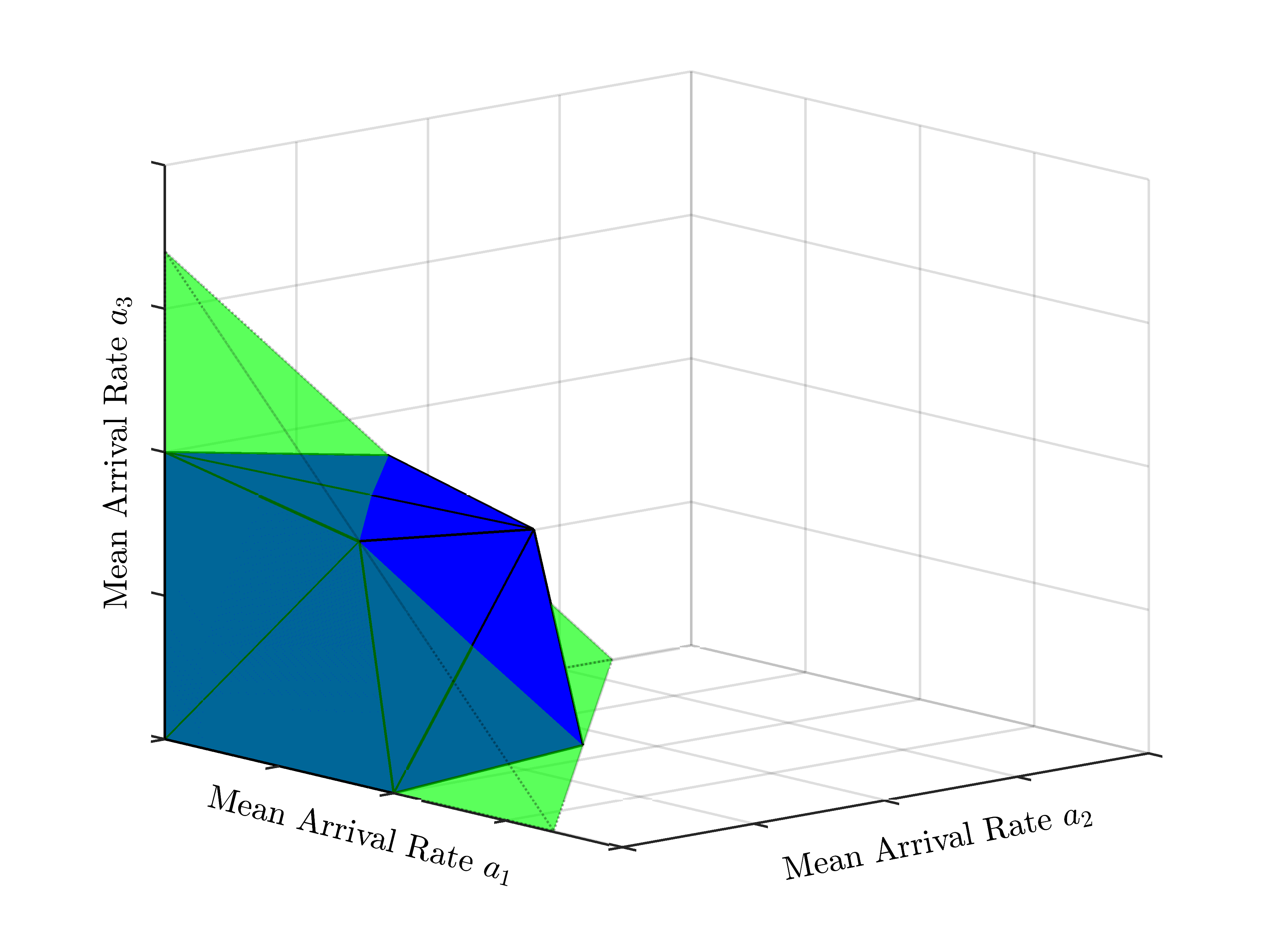
Figure 12: Stability regions of TDMA-SVD (green region) and IA under the imperfect case (blue region) for the symmetric system, where $L_{\text{I}}=N=3$. This illustration represents the case where IA outperforms TDMA-SVD, in which the blue region surpasses (partially) the green region. Note that a similar illustration can be given to compare between IA under the perfect case and TDMA-SVD.

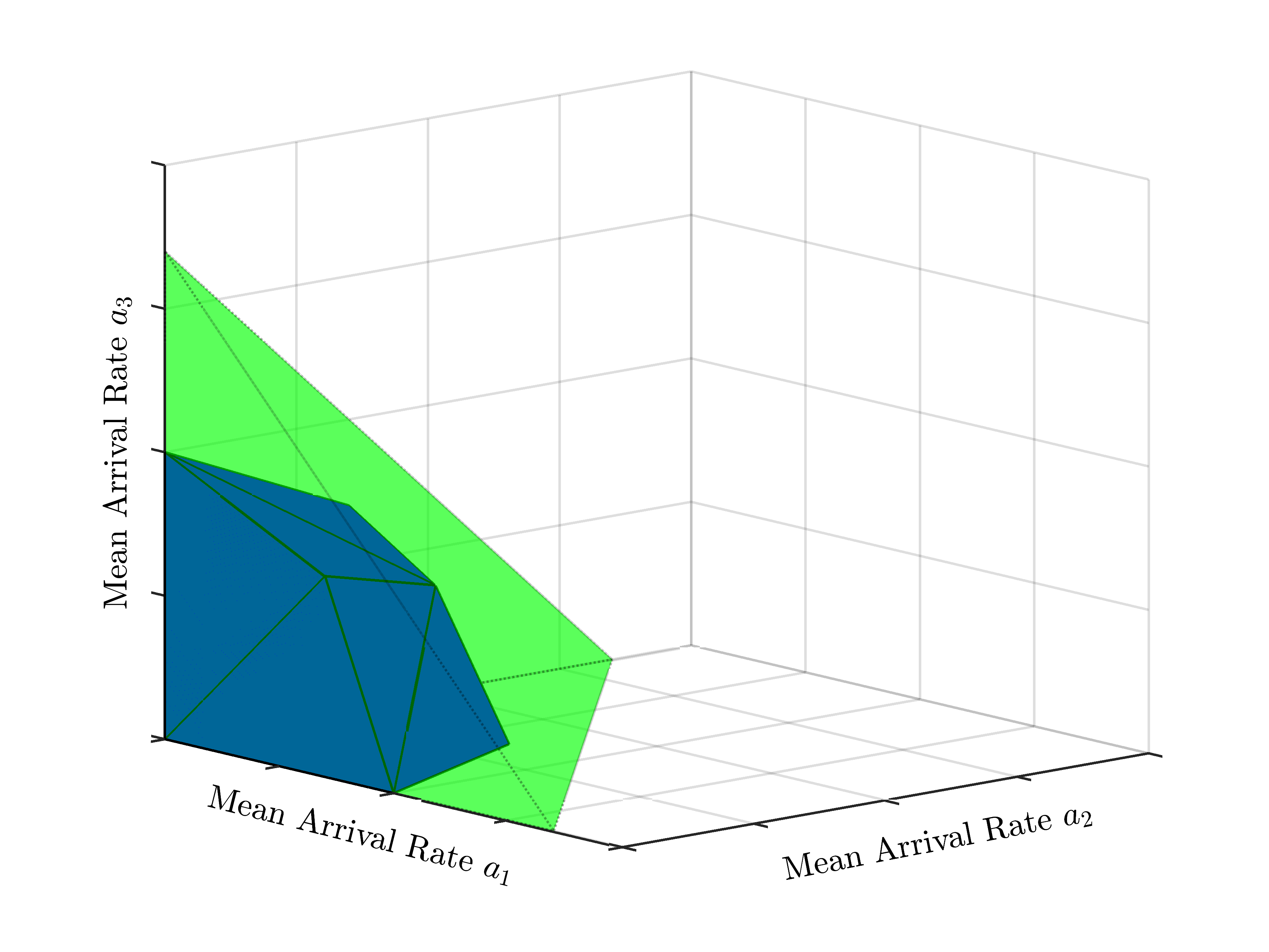
Figure 13: Stability regions of TDMA-SVD (green region) and IA under the imperfect case (blue region) for the symmetric system, where $L_{\text{I}}=N=3$. This illustration represents the case where TDMA-SVD outperforms IA, in which the green region covers the blue region. Note that a similar illustration can be given to compare between IA under the perfect case and TDMA-SVD.

References

- [1] M. Deghel, M. Assaad, and M. Debbah, “Queueing stability and CSI probing of a TDD wireless network with interference alignment,” in Information Theory (ISIT), 2015 IEEE International Symposium on, June 2015, pp. 794–798.
- [2] V. R. Cadambe and S. A. Jafar, “Interference alignment and degrees of freedom of the -user interference channel,” IEEE Trans. Inform. Theory, vol. 54, no. 8, pp. 3425–3441, August 2008.
- [3] J. Thukral and H. Bölcskei, “Interference alignment with limited feedback,” CoRR, vol. abs/0905.0374, 2009. [Online]. Available: http://arxiv.org/abs/0905.0374
- [4] R. Krishnamachari and M. Varanasi, “Interference alignment under limited feedback for MIMO interference channels,” in Information Theory Proceedings (ISIT), 2010 IEEE International Symposium on, June 2010, pp. 619–623.
- [5] M. Rezaee and M. Guillaud, “Limited feedback for interference alignment in the K-user MIMO interference channel,” in Information Theory Workshop (ITW), 2012 IEEE, Sept 2012, pp. 667–671.
- [6] N. Jindal, “MIMO broadcast channels with finite-rate feedback,” Information Theory, IEEE Transactions on, vol. 52, no. 11, pp. 5045–5060, Nov 2006.
- [7] W. Santipach and M. Honig, “Capacity of a multiple-antenna fading channel with a quantized precoding matrix,” Information Theory, IEEE Transactions on, vol. 55, no. 3, pp. 1218–1234, March 2009.
- [8] O. E. Ayach and R. W. Heath, “Interference alignment with analog channel state feedback,” IEEE Trans. Wireless Commun., vol. 11, no. 2, pp. 626–636, February 2012.
- [9] R. Tresch and M. Guillaud, “Cellular interference alignment with imperfect channel knowledge,” in Communications Workshops, 2009. ICC Workshops 2009. IEEE International Conference on, June 2009, pp. 1–5.
- [10] S. Park, O. Simeone, O. Sahin, and S. Shamai, “Performance evaluation of multiterminal backhaul compression for cloud radio access networks,” CoRR, vol. abs/1311.6492, 2013. [Online]. Available: http://arxiv.org/abs/1311.6492
- [11] M. Rezaee, M. Guillaud, and F. Lindqvist, “CSIT sharing over finite capacity backhaul for spatial interference alignment,” in IEEE International Symposium on Information Theory Proceedings (ISIT’13). IEEE, July 2013, pp. 569–573.
- [12] H. Boche and M. Wiczanowski, “The interplay of link layer and physical layer under MIMO enhancement: benefits and challenges,” Wireless Communications, IEEE, vol. 13, no. 4, pp. 48–55, Aug 2006.
- [13] N. McKeown, A. Mekkittikul, V. Anantharam, and J. Walrand, “Achieving 100 percent throughput in an input-queued switch,” Communications, IEEE Transactions on, vol. 47, no. 8, pp. 1260–1267, Aug 1999.
- [14] P. Kumar and S. Meyn, “Duality and linear programs for stability and performance analysis of queuing networks and scheduling policies,” Automatic Control, IEEE Transactions on, vol. 41, no. 1, pp. 4–17, Jan 1996.
- [15] E. Leonardi, M. Mellia, F. Neri, and M. Ajmone Marsan, “Bounds on average delays and queue size averages and variances in input-queued cell-based switches,” in INFOCOM 2001. Twentieth Annual Joint Conference of the IEEE Computer and Communications Societies. Proceedings. IEEE, vol. 2, 2001, pp. 1095–1103 vol.2.
- [16] W. Szpankowski, “Stability conditions for some distributed systems: Buffered random access systems,” Buffered Random Access Systems, Adv. Appl. Probab, vol. 26, pp. 498–515, 1993.
- [17] L. Tassiulas and A. Ephremides, “Stability properties of constrained queueing systems and scheduling policies for maximum throughput in multihop radio networks,” Automatic Control, IEEE Transactions on, vol. 37, no. 12, pp. 1936–1948, Dec 1992.
- [18] M. Neely, E. Modiano, and C. Rohrs, “Power allocation and routing in multibeam satellites with time-varying channels,” Networking, IEEE/ACM Transactions on, vol. 11, no. 1, pp. 138–152, Feb 2003.
- [19] H. Boche and M. Wiczanowski, “Optimization-theoretic analysis of stability-optimal transmission policy for multiple-antenna multiple-access channel,” Signal Processing, IEEE Transactions on, vol. 55, no. 6, pp. 2688–2702, June 2007.
- [20] C. Swannack, E. Uysal-biyikoglu, and G. Wornell, “Low complexity multiuser scheduling for maximizing throughput,” in in the MIMO Broadcast Channel,” in Proc. Allerton Conf. Commun., Contr., and Computing, 2004.
- [21] M. Kobayashi and G. Caire, “An iterative water-filling algorithm for maximum weighted sum-rate of gaussian mimo-bc,” Selected Areas in Communications, IEEE Journal on, vol. 24, no. 8, pp. 1640–1646, Aug 2006.
- [22] C. Wang and R. Murch, “Optimal downlink multi-user mimo cross-layer scheduling using hol packet waiting time,” Wireless Communications, IEEE Transactions on, vol. 5, no. 10, pp. 2856–2862, Oct 2006.
- [23] M. Kobayashi, G. Caire, and D. Gesbert, “Transmit diversity versus opportunistic beamforming in data packet mobile downlink transmission,” Communications, IEEE Transactions on, vol. 55, no. 1, pp. 151–157, Jan 2007.
- [24] M. Kobayashi and G. Caire, “Joint beamforming and scheduling for a multi-antenna downlink with imperfect transmitter channel knowledge,” Selected Areas in Communications, IEEE Journal on, vol. 25, no. 7, pp. 1468–1477, September 2007.
- [25] K. Huang and V. Lau, “Stability and delay of zero-forcing SDMA with limited feedback,” Information Theory, IEEE Transactions on, vol. 58, no. 10, pp. 6499–6514, Oct 2012.
- [26] P. Chaporkar, A. Proutiere, H. Asnani, and A. Karandikar, “Scheduling with limited information in wireless systems,” in Proceedings of the Tenth ACM International Symposium on Mobile Ad Hoc Networking and Computing, ser. MobiHoc ’09. New York, NY, USA: ACM, 2009, pp. 75–84. [Online]. Available: http://doi.acm.org/10.1145/1530748.1530759
- [27] A. Destounis, M. Assaad, M. Debbah, and B. Sayadi, “Traffic-aware training and scheduling for MISO wireless downlink systems,” Information Theory, IEEE Transactions on, vol. 61, no. 5, pp. 2574–2599, May 2015.
- [28] M. B. Stefania Sesia, Issam Toufik, “LTE, the UMTS long term evolution: From theory to practice.” Wiley, 2009.
- [29] E. T. Ar and I. E. Telatar, “Capacity of multi-antenna gaussian channels,” European Transactions on Telecommunications, vol. 10, pp. 585–595, 1999.
- [30] O. El Ayach, A. Lozano, and R. Heath, “On the overhead of interference alignment: Training, feedback, and cooperation,” Wireless Communications, IEEE Transactions on, vol. 11, no. 11, pp. 4192–4203, November 2012.
- [31] C. M. Yetis, T. Gou, S. A. Jafar, and A. H. Kayran, “On feasibility of interference alignment in MIMO interference networks,” IEEE Trans. Signal Processing, vol. 58, no. 9, pp. 4771–4782, September 2010.
- [32] L. Georgiadis, M. J, and R. Tassiulas, “Resource allocation and cross-layer control in wireless networks,” in Foundations and Trends in Networking, 2006, pp. 1–149.
- [33] X. Chen and C. Yuen, “Performance analysis and optimization for interference alignment over mimo interference channels with limited feedback,” Signal Processing, IEEE Transactions on, vol. 62, no. 7, pp. 1785–1795, April 2014.
- [34] B. Jóhannesson and N. Giri, “On approximations involving the beta distribution,” Communications in Statistics-Simulation and Computation, vol. 24, no. 2, pp. 489–503, 1995.
- [35] X. Chen and C. Yuen, “Performance analysis and optimization for interference alignment over MIMO interference channels with limited feedback,” Signal Processing, IEEE Transactions on, vol. 62, no. 7, pp. 1785–1795, April 2014.
- [36] S. Nadarajah and S. Kotz, “On the product and ratio of gamma and beta random variables,” Allgemeines Statistisches Archiv, vol. 89, no. 4, pp. 435–449, 2005. [Online]. Available: http://dx.doi.org/10.1007/s10182-005-0214-9
- [37] H. Bateman, A. Erdélyi, H. van Haeringen, and L. Kok, Tables of integral transforms. McGraw-Hill New York, 1954, vol. 1.
- [38] S. Boyd and L. Vandenberghe, Convex Optimization. New York, NY, USA: Cambridge University Press, 2004.