Lorentz invariant relative velocity and relativistic binary collisions

Abstract

This article reviews the concept of Lorentz invariant relative velocity that is often misunderstood or unknown in high energy physics literature. The properties of the relative velocity allow to formulate the invariant flux and cross section without recurring to non–physical velocities or any assumption about the reference frame. Applications such as the luminosity of a collider, the use as kinematic variable, and the statistical theory of collisions in a relativistic classical gas are reviewed. It is emphasized how the hyperbolic properties of the velocity space explain the peculiarities of relativistic scattering.

I Introduction

In every book on relativistic quantum field theory and particle physics a section or an appendix is necessarily devoted to the formulation of the Lorentz invariant cross section. To fix the ideas we consider the total cross section for binary collisions $1+2\to f$ where $f$ is a final state with 2 or more particles.

The basic quantity that is measured in experiments is the reaction rate, that is the number of events with the final state $f$ per unit volume per unit of time,

$$\mathcal{R}_{f}=\frac{dN_{f}}{dVdt}=\frac{dN_{f}}{d^{4}x}.$$ (1)

The value of the reaction rate is proportional to the number density of particles $n_{1}$ and $n_{2}$ that approach each other with a certain relative velocity, for example an incident beam on a fixed target or two colliding beams. This is the so–called initial (or incident) flux $F$. The physical quantity that gives the intrinsic quantum probability for a transition independent from the details of the initial state is the cross section defined as the ratio $\sigma={\mathcal{R}_{f}}/{F}$.

In nonrelativistic scattering the initial flux is given by

$$F_{\text{nr}}=n_{1}n_{2}v_{r},$$ (2)

where

$$v_{r}=|\boldsymbol{v}_{1}-\boldsymbol{v}_{2}|,$$ (3)

is the nonrelativistic relative velocity.

Since the number of events $N_{f}$ does not depend on the reference frame and $d^{4}x$ is invariant, it is essential that the initial flux $F$ and the cross section $\sigma$ are invariant under proper Lorentz transformations such that their product $\mathcal{R}_{f}$ is invariant. The expressions (2) and (3) are not invariant under Lorentz transformations and are not valid in the relativistic framework.

We start this review, Section II, with a critical discussion of how the relativistic flux is presented in textbooks. This will lead us to review in Section III the properties of the invariant relative velocity and to discuss a simple Lorentz invariant definition of the flux in Section IV. We then review some important applications to the theory of relativistic scattering: the luminosity of a collider in Section V, the use of the invariant relative velocity as kinematic variable in Section VI, and the theory of collisions in a relativistic gas in Section VII. Overall, we shall emphasize how the hyperbolic nature of the relativistic velocity space manifests itself in concrete physical applications.

II The definition of invariant cross section: three problems and a solution

In quantum field theory the invariant rate corresponds to the probability per unit time per unit volume of a single transition $i\to f$, $\mathcal{R}^{\text{th}}_{\text{fi}}=\frac{dP_{\text{fi}}}{dVdt}$ and is given by

$$\mathcal{R}^{\text{th}}_{\text{fi}}=\int\overline{|\mathcal{M}_{\text{fi}}|^{2}}(2\pi)^{4}\delta^{4}(P_{i}-P_{f})\prod_{j=3}^{n}\frac{d^{3}\boldsymbol{p}_{j}}{(2\pi)^{3}2E_{j}}.$$ (4)

Equation (4) refers to the scattering of unpolarized particles, hence the square of the amplitude is summed over the final spins and averaged over the initial spins. With $P_{i}$ and $P_{f}$ we indicate the total 4-momentum of the initial and final states, respectively.

In (4) we use the normalization of one–particle states $\langle p|p^{\prime}\rangle=(2\pi)^{3}2E\delta^{3}(\boldsymbol{p}-\boldsymbol{p}^{\prime})$ both for bosons and fermions, which corresponds to ‘$2E$ particles per unit volume’ instead of ‘one particle per unit volume’. The densities appearing in the flux according to this convention are thus $n=2E$. We shall see that for an experimentalist or in the case of a gas of particles, the densities are something more concrete.

Although in the Introduction we argued that Eq. (2) is not valid in the relativistic framework, the starting point of quantum field theory and particle physics textbooks is nonetheless the nonrelativistic expression

$$F=n_{1}n_{2}\rvert\boldsymbol{v}_{1}-\boldsymbol{v}_{2}\rvert,$$ (5)

where velocities $\boldsymbol{v}_{1}$ and $\boldsymbol{v}_{2}$ are required to be collinear. This includes as particular cases the expression of the flux in the rest frame of massive particles and in the center of momentum frame. We shall discuss in a moment this assumption. Let us proceed and use $\boldsymbol{v}=\boldsymbol{p}/E$ to rewrite Eq. (5) as

$$n_{1}n_{2}\Big{\rvert}\frac{E_{2}\boldsymbol{p}_{1}-E_{1}\boldsymbol{p}_{2}}{E_{1}E_{2}}\Big{\rvert}.$$

Employing $E^{2}=m^{2}+\boldsymbol{p}^{2}$ we find

$$|E_{2}\boldsymbol{p}_{1}-E_{1}\boldsymbol{p}_{2}|$$ (6)

$$=[m^{2}_{2}\boldsymbol{p}_{1}^{2}+m^{2}_{2}\boldsymbol{p}_{2}^{2}-2E_{1}E_{2}\boldsymbol{p}_{1}\cdot\boldsymbol{p}_{2}+2\boldsymbol{p}_{1}^{2}\boldsymbol{p}_{2}^{2}]^{1/2}.$$ (7)

Now we note that

$$\mathcal{F}\equiv\sqrt{(p_{1}\cdot p_{2})^{2}-m^{2}_{1}m^{2}_{2}}=$$

$$[m^{2}_{2}\boldsymbol{p}_{1}^{2}+m^{2}_{2}\boldsymbol{p}_{2}^{2}-2E_{1}E_{2}\boldsymbol{p}_{1}\cdot\boldsymbol{p}_{2}+\boldsymbol{p}_{1}^{2}\boldsymbol{p}_{2}^{2}+(\boldsymbol{p}_{1}\cdot\boldsymbol{p}_{2})^{2}]^{1/2},$$ (8)

where we used again the relativistic energy formula. If the velocities are collinear, the last two terms in (8) are equal and sum to give the last term in (7). In this case the expressions (7) and (8) coincide and the flux (5) becomes

$$F=\frac{n_{1}n_{2}}{E_{1}E_{2}}\mathcal{F}.$$ (9)

The product of the number densities is $n_{1}n_{2}=4E_{1}E_{2}$, hence

$$F=4\mathcal{F}.$$ (10)

This is the most popular form of the flux in particle physics also reported in the review of the Particle Data Group [41].

II.1 Why collinear velocities?

If we start from Eq. (5), the assumption of collinearity is necessary because, taking the velocities along the $z$ axis for example, the expression $E_{1}E_{2}|v_{1_{z}}-v_{2_{z}}|=|E_{2}p_{1_{z}}-E_{1}p_{2_{z}}|$ is at least invariant under boosts along the $z$ axis, even if not under a general Lorentz transformation. This corresponds to the simplification of the last terms in Eq. (8).

The final expression (10) is anyway a Lorentz scalar, hence also valid for noncollinear velocities as can be easily seen in the following way. Dividing Eq. (8) by $E_{1}E_{2}$, the right hand side can be written as

$$\left[\left(\frac{\boldsymbol{p}_{1}}{E_{1}}-\frac{\boldsymbol{p}_{2}}{E_{2}}\right)^{2}+\left(\frac{\boldsymbol{p}_{1}}{E_{1}}\cdot\frac{\boldsymbol{p}_{2}}{E_{2}}\right)^{2}-\left(\frac{\boldsymbol{p}_{1}}{E_{1}}\right)^{2}\left(\frac{\boldsymbol{p}_{2}}{E_{2}}\right)^{2}\right]^{1/2}$$

$$\;=[(\boldsymbol{v}_{1}-\boldsymbol{v}_{2})^{2}+(\boldsymbol{v}_{1}\cdot\boldsymbol{v}_{2})^{2}-\boldsymbol{v}^{2}_{1}\boldsymbol{v}^{2}_{2}]^{1/2}.$$ (11)

Using the vector identity

$$(\boldsymbol{a}\times\boldsymbol{b})^{2}=\boldsymbol{a}^{2}\boldsymbol{b}^{2}-(\boldsymbol{a}\cdot\boldsymbol{b})^{2}$$ (12)

in (11), it follows

$$\frac{\mathcal{F}}{E_{1}E_{2}}=\sqrt{(\boldsymbol{v}_{1}-\boldsymbol{v}_{2})^{2}-{(\boldsymbol{v}_{1}\times\boldsymbol{v}_{2})^{2}}}\equiv\bar{v}.$$ (13)

Therefore for every $\boldsymbol{v}_{1}$ and $\boldsymbol{v}_{2}$ we can write

$$F =n_{1}n_{2}\sqrt{(\boldsymbol{v}_{1}-\boldsymbol{v}_{2})^{2}-(\boldsymbol{v}_{1}\times\boldsymbol{v}_{2})^{2}}.$$ (14)

The collinear flux (5) is just a particular case of the invariant expression (14) when $\boldsymbol{v}_{1}\times\boldsymbol{v}_{2}=0$.

The Møller’s flux

Formula (14) was proposed a long time ago in [37]. In this paper Møller notes that textbooks define (at that time) the cross section in the center of momentum frame with the flux given by Eq. (5) (hence not differently from today). His purpose is to find a general expression valid also for non collinear velocities.

Møller does not derive, but affirms that such an expression is given by Eq. (14) and then prove the invariance. In order to do that, he writes the squared root in (14) as $\frac{B}{E_{1}E_{2}}$, with

$$B=\sqrt{(E_{2}\boldsymbol{p}_{1}-E_{1}\boldsymbol{p}_{2})^{2}-(\boldsymbol{p}_{1}\times\boldsymbol{p}_{2})^{2}}.$$

The squared expressions under the squared root are antisymmetric in the indices 1 and 2. Møller thus introduces the antisymmetric tensor

$$A^{\mu\nu}=p^{\mu}_{1}p^{\nu}_{2}-p^{\nu}_{1}p^{\mu}_{2},$$

and it is easy to see that

$$B=\sqrt{-\frac{1}{2}A^{\mu\nu}A_{\mu\nu}}$$

is a scalar and coincides with $\mathcal{F}$. The flux (14) is then rewritten as

$$F=\frac{n_{1}n_{2}}{E_{1}E_{2}}B.$$ (15)

Since energy is the time component of the 4-momentum and number density is the time component of the 4-current

$$J=(n,n\boldsymbol{v})=n^{0}(\gamma,\gamma\boldsymbol{v})=n^{0}u,$$ (16)

where $n^{0}$ is the number density in rest frame and $u$ the 4-velocity $u=\gamma(1,\boldsymbol{v})$, $u^{2}=1$, $n_{i}$ and $E_{i}$ transform in the same way under Lorentz transformations. The ratio $\frac{n_{1}n_{2}}{E_{1}E_{2}}$ is then a Lorentz invariant quantity. The flux is invariant because is the product of two scalar quantities.

Anyway, neither the derivation we have given, nor the Møller’s paper clarifies how to derive expression (14) from first principles without starting from (5) with collinear velocities.

II.2 ‘Who’ is the relative velocity?

It is important to remark that Møller puts the product $E_{1}E_{2}$ in ratio with the product of densities $n_{1}n_{2}$, not with the scalar $B$. He does not introduce any ‘Møller velocity’ or call relative velocity the quantity $\bar{v}$ defined in (13).

The misleading identification of $\bar{v}=\mathcal{F}/E_{1}E_{2}$ with a relative velocity or a ‘Møller velocity’ is posterior, probably suggested by the deceptive similarity of $F=n_{1}n_{2}\bar{v}$ with the nonrelativistic expression $F_{\text{nr}}=n_{1}n_{2}v_{r}$.

As a matter of fact, in particle physics literature, some authors consider the quantity $\bar{v}$ as the relative velocity that generalizes the nonrelativistic expression $v_{r}$, for others the relative velocity is $v_{r}$. In statistical physics literature [19] and in dark matter literature [18], $\bar{v}$ is called Møller velocity to distinguish it from the relative velocity, which is considered to be given by $v_{r}$ in any case.

The above identification is unfortunate because albeit the product $E_{1}E_{2}\bar{v}$ is a scalar, $\bar{v}$ by itself is not invariant. Even worse, for many configurations and magnitudes of the two velocities, $v_{r}$ and $\bar{v}$ take values larger than the velocity of light, both for massive and massless particles. For example, in the center of momentum frame of two particles with equal masses, we have $v_{r}=\bar{v}=2v_{*}$ and for $v_{*}>0.5$ the ‘relative velocity’ is superluminal.

Explicitly or tacitly, in high energy physics literature is an accepted fact that the relative velocity of two particles can be larger than the velocity of light.

In reality this is a macroscopic violation of the principles of relativity. Fock [16] expresses the point with the clearest words:

In pre-relativistic mechanics the relative velocity of two bodies was defined as the difference of their velocities. Let the velocities of two bodies, both measured in the same frame of reference, be $\bf{u}$ and $\bf{v}$ respectively. Then the velocity of the second body relative to the first used to be defined as $\bf{w}=\bf{v}-\bf{u}$. This definition is invariant with respect to Galileo transformations but not Lorentz transformations. Therefore it is not suitable in the Theory of Relativity and must be replaced by another. The fact that $\bf{w}=\bf{v}-\bf{u}$ has no physical meaning becomes evident by examining the following example. Let the velocities $\bf{u}$ and $\bf{v}$ have opposite directions and have magnitudes near to the speed of light or equal to it. The ‘velocity’ $\bf{w}$ will have a magnitude near or equal to twice the speed of light, which is evidently absurd.

In special relativity every physical velocity must satisfy

$$v^{2}_{1}+v^{2}_{2}+v^{2}_{3}<1$$ (17)

in every inertial frame. Clearly, massless particles propagate at the velocity of light, thus the relative velocity of two photons, or an electron and a photon is equal to 1 in every inertial frame.

Strictly speaking, following Fock, the mathematical expressions $|\boldsymbol{v}_{1}-\boldsymbol{v}_{2}|$ and $\bar{v}$ are not even velocities in special relativity.

II.3 Transformation of densities

The product $n_{1}n_{2}$ is not Lorentz invariant. In fact the densities in a generic frame do not coincide with the proper densities because of the volume contraction, or, from another point of view, densities are only the time component of a 4-vector. Nonetheless, the product $n_{1}n_{2}\bar{v}$ is the physical invariant flux. This means that the true relative velocity is hidden in this expression and some cancellation takes place. We shall see that this is what happens.

II.4 The Landau-Lifschitz solution

An answer to the above problems is given in [32]. Let us rephrase the somewhat cumbersome Landau–Lifschitz reasoning.

They assume that both the cross section and the relative velocity must be defined in the rest frame of one particle, say particle 1 to fix the ideas. In this frame, by definition of rate, we have $\mathcal{R}=\sigma v_{\text{rel}}n_{1}n_{2}=\sigma v_{2}n^{0}_{1}n_{2}$. In another frame, in general, the rate takes the form $\mathcal{R}=An_{1}n_{2}$, with $A$ a factor reducing to $\sigma v_{\text{rel}}$ in the rest frames. We have to find the expression of $A$ in a generic frame.

Since the rate is invariant, the product $An_{1}n_{2}$ must be invariant. Using $n=\gamma n^{0}$, with $n^{0}$ the proper density corresponding to the rest frames, and $\gamma=E/m$, we have

$$An_{1}n_{2}=A\frac{E_{1}}{m_{1}}\frac{E_{2}}{m_{2}}n^{0}_{1}n^{0}_{2}.$$

The masses and the proper densities $n_{0}$ are numbers, thus we must require that $AE_{1}E_{2}=c_{i}$, with $c_{i}$ an invariant. Divide now both sides of the previous equality by the scalar $p_{1}\cdot p_{2}$, thus

$$A\frac{E_{1}E_{2}}{p_{1}\cdot p_{2}}=c^{\prime}_{i},$$

with $c^{\prime}_{i}=c_{i}/p_{1}\cdot p_{2}$ another invariant. In the rest frame of one particle $E_{1}E_{2}/p_{1}\cdot p_{2}=1$ and $A=c^{\prime}_{i}=\sigma v_{\text{rel}}$ by assumption. Hence in a generic frame

$$A=\frac{p_{1}\cdot p_{2}}{E_{1}E_{2}}\sigma v_{\text{rel}}.$$ (18)

In the rest frame of one particle 1 we already said that $v_{\text{rel}}=|\boldsymbol{v}_{2}|$. The 4-momenta are $p_{1}=(m_{1},0)$, $p_{2}=(E_{2},\boldsymbol{p}_{2})$ with scalar product $p_{1}\cdot p_{2}=m_{1}E_{2}$. It follows that $v_{\text{rel}}={|\boldsymbol{p}_{2}|}/{E_{2}}={\sqrt{E^{2}_{2}-m^{2}_{2}}}/{E_{2}}$ can be written as

$$v_{\text{rel}}=\frac{\sqrt{(p_{1}\cdot p_{2})^{2}-m^{2}_{1}m^{2}_{2}}}{p_{1}\cdot p_{2}}.$$ (19)

Using (13) and $p_{1}\cdot p_{2}/E_{1}E_{2}=1-\boldsymbol{v}_{1}\cdot\boldsymbol{v}_{2}$, in terms of velocities Eq. (19) becomes

$$v_{\text{rel}}=\frac{\sqrt{(\boldsymbol{v}_{1}-\boldsymbol{v}_{2})^{2}-(\boldsymbol{v}_{1}\times\boldsymbol{v}_{2})^{2}}}{1-\boldsymbol{v}_{1}\cdot\boldsymbol{v}_{2}}.$$ (20)

From Eq. (18) and (19) the invariant flux is

$$F=n_{1}n_{2}\frac{\cancel{p_{1}\cdot p_{2}}}{E_{1}E_{2}}\frac{\sqrt{(p_{1}\cdot p_{2})^{2}-m^{2}_{1}m^{2}_{2}}}{\cancel{p_{1}\cdot p_{2}}},$$

which gives Eq. (9), or, in terms of velocities,

$$F=n_{1}n_{2}\cancel{(1-\boldsymbol{v}_{1}\cdot\boldsymbol{v}_{2})}\frac{\sqrt{(\boldsymbol{v}_{1}-\boldsymbol{v}_{2})^{2}-{(\boldsymbol{v}_{1}\times\boldsymbol{v}_{2})^{2}}}}{\cancel{1-{\boldsymbol{v}_{1}\cdot\boldsymbol{v}_{2}}}},$$

which coincides with Eq. (14). Landau-Lifshitz thus provide an ab initio derivation of the Møller formula (14). A similar discussion was also given in [46].

We have highlighted the cancellation because is the central point. Formula (14), and its particular case (5), arises because there is the cancellation between the factor ($1-\boldsymbol{v}_{1}\cdot\boldsymbol{v}_{2}$) that comes from the transformation of densities with the same factor in the denominator of the relative velocity. Only a posteriori we can say that the relativistic flux with collinear velocities is given by Eq. (5). The result of the cancellation is an expression which formally looks the nonrelativistic flux, but the relative velocity in the collinear case is

$$v^{\parallel}_{\text{rel}}=\frac{|\boldsymbol{v}_{1}-\boldsymbol{v}_{2}|}{1-\boldsymbol{v}_{1}\cdot\boldsymbol{v}_{2}},$$ (21)

not $|\boldsymbol{v}_{1}-\boldsymbol{v}_{2}|$ as it is generally believed.

What about the ‘Møller velocity’? It is just the numerator of formula (20) or the product of the factor $(1-\boldsymbol{v}_{1}\cdot\boldsymbol{v}_{2})$ with $v_{\text{rel}}$. This explains why it does not have any physical meaning by itself. In the next sections we shall see that leaving such factor and the relative velocity explicitly in the formulas allows for a clearer understanding of relativistic physics.

Actually it is possible to give a much general and simpler formulation than the Landau-Lifschitz’s one without any assumption about reference frames. But before, there are many interesting properties of the relative velocity that is necessary to recall.

III Properties of the invariant relative velocity

If we restore $c$ in (20), the vector product in the numerator and the scalar product in the denominator are divided by $c^{2}$. In the nonrelativistic limit $c\to\infty$, $|\boldsymbol{v}_{i}|\ll c$ they disappear, and $v_{\text{rel}}$ reduces to $v_{r}$. When one (or both) velocity is $c$, then $v_{\text{rel}}=c$, while when both are smaller than $c$ then $v_{\text{rel}}<c$. All the physical requirements are satisfied.

Formula (20) can be found in some books on relativity but to our knowledge cannot be found in any particle physics or quantum field theory book. Up to a minus sign in the numerator and in the denominator, this is the well known Einstein’s rule for the composition of velocities already written in the 1905’s paper [15].

If one prefers to reason in terms of Lorentz transformations, the easiest way is to take $S$ as the laboratory frame where $\boldsymbol{v}_{1}$ and $\boldsymbol{v}_{2}$ are given, and $S_{1}$ the rest frame of particle 1. $S_{1}$ moves with velocity $\boldsymbol{v}_{1}$ with respect to $S$, hence the velocity $\boldsymbol{v}_{21}$ of particle 2 in $S_{1}$, that is the relative velocity, is found by applying a boost $B(\boldsymbol{v}_{1})$ to $\boldsymbol{v}_{2}$. One gets, see for example [16], [47],

$$\boldsymbol{v}_{21}=\frac{\boldsymbol{v}_{2}-\boldsymbol{v}_{1}-(\gamma_{1}-1)(1-\frac{\boldsymbol{v}_{1}\cdot\boldsymbol{v}_{2}}{\boldsymbol{v}^{2}_{1}})\boldsymbol{v}_{1}}{\gamma_{1}(1-\boldsymbol{v}_{1}\cdot\boldsymbol{v}_{2})}.$$ (22)

By taking $S_{2}$ as the rest frame of particle 2, with similar reasoning, instead we have

$$\boldsymbol{v}_{12}=\frac{\boldsymbol{v}_{1}-\boldsymbol{v}_{2}-(\gamma_{2}-1)(1-\frac{\boldsymbol{v}_{1}\cdot\boldsymbol{v}_{2}}{\boldsymbol{v}^{2}_{2}})\boldsymbol{v}_{2}}{\gamma_{2}(1-\boldsymbol{v}_{1}\cdot\boldsymbol{v}_{2})}.$$ (23)

Differently from the nonrelativistic case where $\boldsymbol{v}_{12}=-\boldsymbol{v}_{21}$, the vectors $\boldsymbol{v}_{12}$ and $\boldsymbol{v}_{21}$ belong to different directions that differ by a spatial rotation. What is important for scattering theory is that the magnitude of the two vectors is the same and symmetrical in indices 1 and 2, being equal to the relative velocity (20)

$$|\boldsymbol{v}_{12}|=|\boldsymbol{v}_{21}|=v_{\text{rel}},$$ (24)

as can be verified with direct calculation.

III.1 Metric and hyperbolic properties

In nonrelativistic physics the vectors $\bm{v}=(v_{1},v_{2},v_{3})$ are points of the Euclidean 3-dimensional velocity space $\mathcal{V}_{\text{nr}}$. The relative velocity ${v}_{\textit{r}}=\rvert\boldsymbol{v}_{1}-\boldsymbol{v}_{2}\rvert$ is invariant under Galileo transformations and coincides with the Euclidean distance between the two points of $\mathcal{V}_{\text{nr}}$,

$$v_{r}=\rho_{E}.$$ (25)

In special relativity the velocity space $\mathcal{V}_{SR}$ is subject to the constraint (17). The space $\mathcal{V}_{SR}$ is given by the points in the interior of sphere of unit radius, in natural units. As it is well known, this is a Lobachevsky-Bolyai hyperbolic space with constant negative curvature [16], [32].

Using Eq. (20) we can calculate the relative velocity between two infinitesimally near points $\boldsymbol{v}$ and $\boldsymbol{v}+d\boldsymbol{v}$. This corresponds to the Riemann metric

$$d\rho^{2}_{H}=\frac{(d\boldsymbol{v})^{2}-(\boldsymbol{v}\times d\boldsymbol{v})^{2}}{(1-\boldsymbol{v}^{2})^{2}},$$ (26)

where the subscript $H$ stands for hyperbolic. As shown in [16], the geodesics of $\mathcal{V}_{SR}$ are straight lines and the points of the segment between $\boldsymbol{v}_{1}$ and $\boldsymbol{v}_{2}$ along the geodesic can be parametrized by linear relations as

$$\boldsymbol{v}_{\lambda}=\boldsymbol{v}_{1}+\lambda(\boldsymbol{v}_{2}-\boldsymbol{v}_{1}),$$ (27)

with $\lambda$ a continuous parameter varying in the interval $[0,1]$. Using (27) in (26) we find the line element

$$d\rho_{H}=\frac{\bar{v}\,d\lambda}{1-\boldsymbol{v}^{2}_{\lambda}}.$$ (28)

The length of the segment gives the distance between the two points of $\mathcal{V}_{SR}$. Performing the integration we find

$$\rho_{H}=\int^{1}_{0}\frac{\bar{v}\,d\lambda}{1-\boldsymbol{v}^{2}_{\lambda}}=\frac{1}{2}\ln\left(\frac{1+v_{\text{rel}}}{1-v_{\text{rel}}}\right).$$ (29)

This is equal to $\tanh^{-1}({v_{\text{rel}}})$; hence, the relation between the relative velocity and the distance is

$$v_{\text{rel}}=\tanh\rho_{H},$$ (30)

which represents the relativistic analogous of (25).

Every velocity in $\mathcal{V}_{SR}$ can be thought as a relative velocity with respect to the origin $O$ with magnitude given by the distance from the origin. In physics this distance is called rapidity, and is indicated commonly with $y$ or $\eta$. From (30) we have the usual relations

$$v=\tanh y,\;\;\gamma=\cosh y,\;\;v\gamma=\sinh y.$$ (31)

We now eliminate the vector product in (20) using the identity (12),

$$v_{\text{rel}}=\sqrt{1-\frac{(1-\boldsymbol{v}_{1}^{2})(1-\boldsymbol{v}^{2}_{2})}{(1-\boldsymbol{v}_{1}\cdot\boldsymbol{v}_{2})^{2}}},$$ (32)

and associate the Lorentz factor to $v_{\text{rel}}$,

$$\gamma_{{\text{r}}}=\frac{1}{\sqrt{1-v^{2}_{\text{rel}}}}.$$ (33)

From (32) and (33) it follows the fundamental relation

$$\gamma_{\text{r}} =\gamma_{1}\gamma_{2}(1-\boldsymbol{v}_{1}\cdot\boldsymbol{v}_{2}).$$ (34)

If $\theta$ is the angle between $\boldsymbol{v}_{1}$ and $\boldsymbol{v}_{2}$, then Eq. (34) can be written as

$$\cosh y_{\text{r}}=\cosh y_{1}\cosh y_{2}-\sinh y_{1}\sinh y_{2}\cos\theta,$$ (35)

which is the cosine rule of hyperbolic geometry. When the velocities are collinear, this give the well known fact that rapidities sum up $y=y_{1}\mp y_{2}$.

In Figure 1 the blue segment passing for the origin describes the scattering of two massive particles with collinear velocities with magnitudes $\boldsymbol{v}_{1}$ and $\boldsymbol{v}_{2}$. Using (29), the distance between the velocities 1 and 2 is the sum of the lengths $\rho_{1O}$ and $\rho_{2O}$

$$\frac{1}{2}\ln\left(\frac{1+v_{\text{rel}}}{1-v_{\text{rel}}}\right)=\frac{1}{2}\ln\left(\frac{1+v_{1}}{1-v_{1}}\right)+\frac{1}{2}\ln\left(\frac{1+v_{2}}{1-v_{2}}\right),$$

which gives

$$v_{\text{rel}}=\frac{v_{1}+v_{2}}{1+v_{1}v_{2}}.$$ (36)

The same result is obtained by (21) orienting the collision axis along $\boldsymbol{v}_{1}$ and taking $\boldsymbol{v}_{2}$ in the opposite direction.

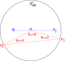
Figure 1: The hyperbolic plane of velocity space represented by the Beltrami-Klein interior disk model of radius 1. The blue segment is relative to two massive particles colliding collinearly. The red triangle describes the scattering of two ultrarelativistic particles colliding with angle $\theta$ in the laboratory.

The metric (26) also determines the angles in velocity space [16],

$$\cos\theta_{ij}=$$

$$\frac{(\boldsymbol{v}_{i}-\boldsymbol{v}_{k})\cdot(\boldsymbol{v}_{j}-\boldsymbol{v}_{k})-(\boldsymbol{v}_{i}\times\boldsymbol{v}_{k})\cdot(\boldsymbol{v}_{j}\times\boldsymbol{v}_{k})}{\sqrt{(\boldsymbol{v}_{i}-\boldsymbol{v}_{k})^{2}-(\boldsymbol{v}_{i}\times\boldsymbol{v}_{k})^{2}}\sqrt{(\boldsymbol{v}_{j}-\boldsymbol{v}_{k})^{2}-(\boldsymbol{v}_{j}\times\boldsymbol{v}_{k})^{2}}},$$ (37)

where angles are the vertices of the velocity triangle individuated by the points $\boldsymbol{v}_{1}$, $\boldsymbol{v}_{2}$ and $\boldsymbol{v}_{3}$, which must be taken in ciclic permutation in Eq. (37).

In Figure 1 we consider the example of scattering of ultrarelativistic or massless particles with velocities $\boldsymbol{v}_{1}=\hat{v}_{1}$ and $\boldsymbol{v}_{2}=\hat{v}_{2}$ in the laboratory frame at rest identified by the origin with velocity $\boldsymbol{v}_{3}=0$. Two vertices of the red triangle are at infinity and the sides are three relative velocities equal to 1, that is of infinite length. From formula (37) it is easy to see that the two angles at the ideal vertices, $\theta_{23}$ and $\theta_{31}$, are zero, while the angle at the origin $\theta_{12}$ is equal to the angle $\cos\theta=\hat{v}_{1}\cdot\hat{v}_{2}$ individuated by the velocities in the laboratory. In hyperbolic geometry the angles determine the sides of the triangle and their sum is less than $\pi$ by an amount given by the hyperbolic defect $\delta=\pi-(\theta_{12}+\theta_{13}+\theta_{23})$. The defect gives the area of the triangle $A=K^{2}\delta$ where $K=1/\sqrt{-k}=1$ being $k=-1$ the gaussian curvature. The area of the red triangle in Figure 1 is thus given by $A=\delta=\pi-\theta$.

III.2 Manifestly invariant representations

Since $v_{\text{rel}}$ is Lorentz invariant it can be written in terms of scalar products of various 4-vectors.

In terms of the 4-velocity $u=\gamma(1,\boldsymbol{v})$, $u^{2}=1$, we have

$$v_{\text{rel}} =\frac{\sqrt{(u_{1}\cdot u_{2})^{2}-1}}{u_{1}\cdot u_{2}}.$$ (38)

The 4-momentum representation is given by (19), and in terms of the 4-current (16) we obtain

$$v_{\text{rel}} =\frac{\sqrt{(J_{1}\cdot J_{2})^{2}-(J_{1})^{2}(J_{2})^{2}}}{J_{1}\cdot J_{2}}.$$ (39)

Another useful formula is found introducing the Mandelstam variable $s=(p_{1}+p_{2})^{2}$,

$$v_{\text{rel}}=\frac{\sqrt{\lambda(s,m^{2}_{1},m^{2}_{2})}}{s-(m^{2}_{1}+m^{2}_{2})},$$ (40)

where we used the triangular function

$$\lambda(s,m^{2}_{1},m^{2}_{2})=[s-(m_{1}+m_{2})^{2}][s-(m_{1}-m_{2})^{2}].$$ (41)

For example the Mandelstam representation gives $s$ as a function of ${v}_{\text{rel}}$ through the Lorentz factor $\gamma_{\text{r}}$

$$s=(m_{1}-m_{2})^{2}+2m_{1}m_{2}(1+\gamma_{\text{r}}),$$ (42)

which is useful for cross section calculations. Also the Lorentz factor can be written in terms of invariants as

$$\gamma_{\text{r}} =u_{1}\cdot u_{2}=\frac{p_{1}\cdot p_{2}}{m_{1}m_{2}}=\frac{J_{1}\cdot J_{2}}{n^{0}_{1}n^{0}_{2}}=\frac{s-(m^{2}_{1}+m^{2}_{2})}{2m_{1}m_{2}}.$$ (43)

Concluding this section we want to emphasize that the connection with the metric properties of the velocity space given by Eq. (25) and Eq. (29) shows that the relative velocity is a concept that is a logical consequence of the relativity principle. The distance, hence the relative velocity, is a number that does not depend on the coordinate system or reference frame, both in the nonrelativistic and in the relativistic case.

IV Lorentz invariant definition of flux

Let us now go back to the incident flux and present how the Landau–Lifschitz reasoning can be made simpler.

The nonrelativistic expression (2) can only by used as a limit to which the new expression reduces in the nonrelativistic limit. The product $n_{1}n_{2}$ must be replaced by some Lorentz scalar that reduces to $n_{1}n_{2}=n^{0}_{1}n^{0}_{2}$. The number densities are the time component of the 4-current (16), hence we are led to take the scalar product

$$J_{1}\cdot J_{2}=n_{1}n_{2}(1-\boldsymbol{v}_{1}\cdot\boldsymbol{v}_{2})=\frac{n_{1}}{\gamma_{1}}\frac{n_{2}}{\gamma_{2}}\gamma_{\text{r}}=n^{0}_{1}n^{0}_{2}\gamma_{\text{r}},$$

where we used Eq. (34). This is the only scalar that can be formed with two 4-currents and presents the correct nonrelativistic limit. Obviously $v_{\text{rel}}$ takes the place of $v_{r}$. It follows that the natural definition of the relativistic invariant flux is

$$F=(J_{1}\cdot J_{2})v_{\text{rel}}.$$ (44)

This expression is a Lorentz scalar at sight and does not rely on the rest frame or the center of momentum frame. For massless particles the velocity vector becomes the unitary vector in the direction of propagation and when at least one massless particle is involved in the scattering then $v_{\text{rel}}=1$. For two massless particles, say two photons, the flux reads $F=n_{1}n_{2}(1-\cos\theta)$, with $\theta$ the angle between $\hat{k}_{1}$ and $\hat{k}_{2}$. For collisions of a massless with a massive particle, $F=n_{1}n_{2}(1-v_{2}\cos\theta)$.

When computing cross sections in quantum field theory, the 4-momentum representation (19) is more useful. We can write

$$F=4(p_{1}\cdot p_{2})v_{\text{rel}},$$ (45)

and when at least one massless particle is involved $F=4(p_{1}\cdot p_{2})$. Clearly expression (10) is only one of the many ways the invariant flux (44) can be explicitly written. For example, using the Mandelstam variable representation one easily finds the well known expression $F=2\sqrt{\lambda(s,m^{2}_{1},m^{2}_{2})}$.

While formula (44) explicitly displays the invariance property, in order to highlight the physical content it is more useful write

$$F=n_{1}n_{2}k_{\text{r}}v_{\text{rel}},$$ (46)

where we have defined the hyperbolic correlation factor

$$k_{\text{r}}=1-\boldsymbol{v}_{1}\cdot\boldsymbol{v}_{2}=\frac{\gamma_{\text{r}}}{\gamma_{1}\gamma_{2}}=\frac{\cosh y_{\text{r}}}{\cosh y_{1}\cosh y_{2}}=\frac{p_{1}\cdot p_{2}}{E_{1}E_{2}}.$$ (47)

The relative velocity (20) hence enters two times in the incident flux: explicitly as a factor and implicitly through $k_{\text{r}}$ that is nothing but the hyperbolic cosine rule given by Eqs. (34) and (35). The hyperbolic correlation factor $k_{\text{r}}$ is not a scalar, only the product $n_{1}n_{2}k_{\text{r}}$ is Lorentz invariant, and attains the maximum value of 2 for example in the case of head on collinear scattering of two photons.

V Flux and luminosity at colliders

We now discuss how experimentalists in high energy particle physics use the concepts of invariant cross section and flux.

In collider physics it is common to consider the rate integrated over the interaction volume. Using the expression Eq. (46) for the flux we have

$$\frac{dN_{f}}{dt}=\sigma\int dVn_{1}n_{2}k_{\text{r}}v_{\text{rel}}=\sigma\mathcal{L}(t),$$ (48)

which defines the instantaneous luminosity $\mathcal{L}(t)$. The integrated luminosity $\mathcal{L}_{\text{int}}=\int dt\mathcal{L}(t)$ gives the total number of expected events $N_{f}=\sigma\mathcal{L}_{\text{int}}$ in a certain running time.

In storage rings like the Large Hadron Collider (LHC) the beams are constituted by bunches with n particles and Gaussian shape characterized by spatial dispersions $\sigma_{x},\sigma_{y},\sigma_{z}$ (root mean squared deviations) along the three directions. Assume further that the beams move along the $z$ axis in opposite directions with ultrarelativistic velocity $v\sim 1$ and produce head-on collisions at the origin of the $z=0$ as in Figure 2. The number densities are thus given by

$$n_{\pm}(\boldsymbol{x},t)=\frac{\texttt{n}}{(2\pi)^{3/2}\sigma_{x}\sigma_{y}\sigma_{z}}e^{-(\frac{x^{2}}{2\sigma^{2}_{x}}+\frac{y^{2}}{2\sigma^{2}_{y}}+\frac{(z\pm vt)^{2}}{2\sigma^{2}_{z}})}.$$ (49)

The luminosity is then

$$\mathcal{L}_{\parallel}(t)=fN_{b}\int d^{3}\boldsymbol{x}\,n_{+}(\boldsymbol{x},t)n_{-}(\boldsymbol{x},t)k_{\text{r}}v_{\text{rel}},$$ (50)

where we have multiplied by the revolution frequency $f$ and the number of bunches $N_{b}$. The parallel symbol indicate the collinear beams. Performing the Gaussian integrations in $x$, $y$, $s=vt$, we obtain the well known result also reported by the Particle Data Group [41]

$$\mathcal{L}_{\parallel}(t)=2\frac{\texttt{n}_{1}\texttt{n}_{2}fN_{b}}{8\pi\sigma_{x}\sigma_{y}}.$$ (51)

The factor 2 arises because for ultrarelativistic particles $v\simeq 1$, $v_{\text{rel}}\simeq 1$ and the velocities correlation factor for this configuration is $k_{\text{r}}\simeq 2$, thus $k_{\text{r}}v_{\text{rel}}\simeq 2$.

In reality at the LHC beams are not collinear but there is an angle $\theta$ between them. Collider physicist prefer to use the complementary angle $\phi=\pi-\theta$, called crossing angle, see Figure 2. The crossing angle is necessary to confine the interaction region and to avoid unwanted collisions and reduce other effects, see for example [26]. While at LHC the crossing angle is small, around 300 $\mu$rad, at the old Intersecting Storage Ring at CERN, where beams were unbunched, it was about 18^∘.

The hyperbolic correlation factor with crossing angle and ultrarelativistic velocities reads

$$k_{\text{r}}\simeq 1-\cos\theta=1+\cos\phi=2\cos^{2}\frac{\phi}{2}.$$ (52)

If the beams are contained in the $x,z$ plane with $\sigma_{z}\gg\sigma_{x},\sigma_{y}$, see Figure 2, the calculation gives [26]

$$\mathcal{L}(t,\phi)=\mathcal{L}_{\parallel}(t)S(\phi),$$ (53)

where

$$S(\phi)=\frac{1}{\sqrt{1+(\frac{\sigma_{z}}{\sigma_{x}}\tan\frac{\phi}{2})^{2}}}$$ (54)

is the reduction factor. For example, at the LHC, the crossing angle is $\phi=285$ $\mu$rad and $\sigma_{z}=7.7$ cm, $\sigma_{x}\simeq 16.7$ $\mu$m, that give $S=0.835$ [26].

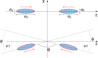
Figure 2: Schematic representation of two bunches in a collinear head-on collision, top figure, and collision with a crossing angle $\phi$, bottom figure.

Note that the crossing angle $\phi$ in the laboratory is equal to the hyperbolic defect of the velocity triangle in velocity space of Figure 1.

At this point it is necessary to make two remarks.

The quantity $A=4\pi\sigma_{x}\sigma_{y}$ that appears in Eq. (51), or $A/S(\phi)$ in Eq. (53), can be considered as an effective cross sectional area of the bunches transverse to the plane that contains the beams, but this quantity depends on the details of the machine and has nothing to do with the theoretical cross section as we argued in footnote 3.

The crossing angle affects the luminosity $\mathcal{L}_{\phi}$ and the number of observed events $\dot{N}_{f}$ but not the ratio, that is the extracted cross section $\sigma_{\text{exp}}=\dot{N}_{f}/\mathcal{L}_{\phi}$, which is an invariant quantity. The theorist does not have to care about the fact that real beams have a crossing angle if the cross section $\sigma^{\text{th}}=\mathcal{R}^{\text{th}}_{f}/F$ is invariant. For this reason the flux must be invariant under general Lorentz transformations and not only under boosts along a fixed direction. The invariant cross section can be calculated in any frame and compared with $\sigma_{\text{exp}}$.

VI Relative velocity as kinematic variable

The relative velocity $v_{\text{rel}}$ and the Lorentz factor $\gamma_{\text{r}}$ are good variables to express the invariant cross section as much as scalar product of 4-momenta, Mandelstam variables or rapidity. For a general example we consider the quantum electrodynamics processes $e^{+}e^{-}\to\gamma\gamma$, pair annihilation, and its inverse $\gamma\gamma\to e^{+}e^{-}$, pair creation.

The total annihilation cross section, see for example [8], can be written as a function of the variable $\tau={s}/{4m^{2}}$ as

$$\sigma_{\text{ann}}(\tau)=\frac{\sigma_{0}}{2\tau^{2}(\tau-1)} \left[(\tau^{2}+\tau-\frac{1}{2})\ln\frac{\sqrt{\tau}+\sqrt{\tau-1}}{\sqrt{\tau}-\sqrt{\tau-1}}\right.$$

$$\left.-(\tau+1)\sqrt{\tau}\sqrt{\tau-1}\right],$$ (55)

where $\sigma_{0}=\pi\alpha^{2}/m^{2}$, $\alpha$ the fine structure constant and $m$ the electron’s mass. Using Eq. (42) with $m_{1}=m_{2}=m$ we obtain

$$s=2m^{2}(1+\gamma_{\text{r}}),\;\;\;\tau=\frac{1}{2}(1+\gamma_{\text{r}}),$$ (56)

and the cross section can be written as

$$\sigma_{\text{ann}}(\gamma_{\text{r}})=\frac{\sigma_{0}}{1+\gamma_{\text{r}}} \left[\frac{\gamma^{2}_{\text{r}}+4\gamma_{\text{r}}+1}{\gamma^{2}_{\text{r}}-1}\ln(\gamma_{\text{r}}+\sqrt{\gamma^{2}_{\text{r}}-1})\right.$$

$$\left.-\frac{\gamma_{\text{r}}+3}{\sqrt{\gamma^{2}_{\text{r}}-1}}\right].$$ (57)

This expression is valid in any frame. In the rest frame of the electron to fix the ideas, the relative velocity coincides with positrons velocity $v_{+}$, hence

$$v_{\text{rel}}(v_{+})=v_{+},\;\;\;\;\gamma_{\text{r}}(v_{+}) =\gamma(v_{+}).$$ (58)

The cross section in the rest frame of the electron is thus given by the same Eq. (57), with $\gamma_{\text{r}}$ replaced by $\gamma(v_{+})$.

In the center of momentum frame instead Eq. (20) gives

$$v_{\text{rel}}(v_{*}) =\frac{2v_{*}}{1+v^{2}_{*}},$$ (59)

with Lorentz factor

$$\gamma_{\text{r}}(v_{*}) =\frac{1+v^{2}_{*}}{1-v^{2}_{*}}.$$ (60)

Substituting (60) into Eq. (57) we find

$$\sigma_{\text{ann}}(v_{*})=\sigma_{0}\frac{1-v^{2}_{*}}{4v_{*}}\left[\frac{3-v^{4}_{*}}{v_{*}}\ln\frac{1+v_{*}}{1-v_{*}}-2(2-v^{2}_{*})\right].$$ (61)

In this way we have obtained the known formula [8] using only the relative velocity.

The cross section of the inverse process [8] is related to Eq. (61) by

$$\sigma_{\text{pair}}(v_{*})=2v^{2}_{*}\sigma_{\text{ann}}(v_{*}).$$ (62)

In order to find the expression valid in any frame we invert Eq. (60)

$$v^{2}_{*}=\frac{\gamma_{\text{r}}-1}{\gamma_{\text{r}}+1}=\frac{\tau-1}{\tau}=1-\frac{2m^{2}}{k_{1}\cdot k_{2}},$$ (63)

where $k_{i}$ are the 4-momenta of the colliding photons. For example, using $\tau$ as variable, we can write

$$\sigma_{\text{pair}}(\tau)=2\frac{\tau-1}{\tau}\sigma_{\text{ann}}(\tau).$$ (64)

In the nonrelativistic limit $v_{\text{rel}}\sim v_{r}\ll 1$, and the expansion of (57) in powers of the relative velocity reads

$$\sigma^{\text{nr}}_{\text{ann}}(v_{\text{rel}})\sim\sigma_{0}(\frac{1}{v_{\text{rel}}}-\frac{3}{20}v^{3}_{\text{rel}}-\frac{11}{105}v^{5}_{\text{rel}}+...).$$ (65)

The expansion in terms of $v_{+}$ in the rest frame of the electron has the same coefficients. Instead, the expansion of (61) to the same order for small $v_{*}$ is

$$\sigma^{\text{nr}}_{\text{ann}}(v_{*})\sim\sigma_{0}(\frac{1}{2v_{*}}+\frac{v_{*}}{2}-\frac{6}{5}v^{3}_{*}+\frac{26}{105}v^{5}_{*}+...).$$ (66)

Both expansions follow the behavior $\sigma\propto\sum_{\ell}a_{\ell}v^{2\ell-1}$ as it is expected for inelastic exothermic processes at low energy. At very low velocities the cross section is dominated by the $\ell=0$ partial wave or $S$-wave. Anyway the coefficients are different, in particular in (65) the one corresponding to $\ell=1$ is zero. Note that (59) has an expansion in odd powers of $v_{*}$

$$v_{\text{rel}}=2v_{*}(1-v^{2}_{*}+v^{4}_{*}-v^{6}_{*}+...),$$ (67)

while

$$\frac{1}{v_{\text{rel}}}=\frac{1}{2v_{*}}+\frac{v_{*}}{2},$$ (68)

has only two terms. In order to obtain (66) from (65) it is necessary to substitute (68) in the first term of (65) and to take powers of (67) keeping all the terms of the same order. For example, $v^{3}_{\text{rel}}\sim 8v^{3}_{*}-24v^{5}_{*}$ gives the term in $v^{3}_{*}$ and a contribution to the order $v^{5}_{*}$ that must be summed to $v^{5}_{\text{rel}}\sim 32v^{5}_{*}$. In this way the expansion (66) is recovered.

If incorrectly we used the ‘Møller velocity’ $\bar{v}_{*}=2v_{*}$ in $\sigma^{\text{nr}}_{\text{ann}}(v_{\text{rel}})$, we would obtain wrong cross section and expansion in the center of mass frame. In terms of $s$ we have $\bar{v}_{*}=2\sqrt{1-4m^{2}/s}$, which gives the relation

$$s=\frac{4m^{2}}{1-\frac{\bar{v}^{2}_{*}}{4}}\sim 4m^{2}+m^{2}v^{2}_{r}+\frac{m^{2}}{4}v^{4}_{r}++\frac{m^{2}}{16}v^{6}_{r}+...,$$ (69)

where the expansion corresponds to the nonrelativistic limit $\bar{v}_{*}\sim v_{r}\ll 1$. This is different from the expansion of (56)

$$s\sim 4m^{2}+m^{2}v^{2}_{r}+\frac{3}{4}m^{2}v^{4}_{r}+\frac{5}{8}m^{2}v^{6}_{r}+...,$$ (70)

which is the correct expansion of $s$ to use in the cross section to obtain the nonrelativistic limit. The misuse of the ‘Møller velocity’ thus can also be source of errors. Examples in dark matter phenomenology are discussed in [12].

VII Relative velocity and relativistic collisions in gases

The hyperbolic correlation factor $k_{\text{r}}$ plays a fundamental role also in the theory of collisions in a relativistic gas. We consider an ideal gas composed of two species of particles with mass $m_{1}$ and $m_{2}$ in thermal equilibrium at a given temperature $T$ and work in the frame where the gas is at rest as a whole, the local rest frame or comoving frame. Before discussing the relativistic gas it is useful to briefly review the nonrelativistic case.

In kinetic theory the number density is determined by the Boltzmann one particle phase space distribution $f^{\text{eq}}=\exp(-E/T)$, $E=\boldsymbol{p}^{2}/2m$, by the integral $n=g/(2\pi)^{3}\int d^{3}\boldsymbol{p}f^{\text{eq}}$,

$$n^{\text{eq}}=g\left(\frac{mT}{2\pi}\right)^{3/2}e^{-m/T},$$ (71)

with $g$ degrees of freedoms of the particle.

It is well known, see for example [33], that the probability density function of the relative velocity $v_{r}$ such that $\int^{\infty}_{0}dv_{r}P(v_{{r}})=1$ is given by

$$P(v_{{r}})=\sqrt{\frac{2}{\pi}}\left(\frac{\mu}{T}\right)^{3/2}{v}^{2}_{{r}}\,e^{-\frac{\mu}{T}\frac{v_{r}^{2}}{2}},$$ (72)

where $\mu=m_{1}m_{2}/(m_{1}+m_{2})$ is the reduced mass. The mean value $\int^{\infty}_{0}dv_{r}P(v_{r})v_{r}$ of $v_{r}$ is given by

$$\langle v_{r}\rangle_{P}=\sqrt{\frac{8T}{\pi\mu}},$$ (73)

and, being $\sigma_{\text{nr}}$ a nonrelativistic cross section that is function of $v_{r}$, the averaged rate is then

$$\langle\mathcal{R}\rangle=\frac{n^{\text{eq}}_{1}n^{\text{eq}}_{2}}{j_{12}}\langle\sigma_{\text{nr}}v_{r}\rangle_{P},\;\;j_{12}=1+\delta_{12},$$ (74)

where $\delta_{12}$ is the Kronecker’s delta and the factor $j_{12}$ must be inserted to avoid double counting when the 1 and 2 are the same specie. The so-called thermal averaged cross section is then

$$\langle\sigma_{\text{nr}}v_{r}\rangle_{P}=\sqrt{\frac{2}{\pi}}\left(\frac{\mu}{T}\right)^{3/2}\int^{\infty}_{0}dv_{r}{v}^{2}_{{r}}\,e^{-\frac{\mu}{T}\frac{v_{r}^{2}}{2}}\sigma_{\text{nr}}v_{r}.$$ (75)

Formula (75) is commonly used for the calculation of abundances of dark matter particles that decoupled at a temperature when they were nonrelativistic, see for example [22]. Instead, expressed as a function of the relative kinetic energy $E=1/2\mu v^{2}_{r}$, Eq. (75) takes the form

$$\langle\sigma_{\text{nr}}v_{r}\rangle_{P} =\sqrt{\frac{8}{\pi\mu T^{3}}}\int^{\infty}_{0}dE\,E\,e^{-\frac{E}{T}}\,\sigma_{\text{nr}}(E),$$ (76)

which, for example, is used for calculating nuclear reaction rates in the Sun [1] and rates in big bang nucleosynthesis [27].

VII.1 The relativistic classical gas

There are other physical problems, for example the calculation of abundances of relics that decoupled when they were relativistic, the calculation of particle yields in ultrarelativistic ion collisions and reaction rates in astrophysical plasmas where the nonrelativistic approximation is not good.

The relativistic generalization of the Boltzmann distribution, also known as Jüttner distribution [19], [14], is

$$f^{\text{eq}}=\exp({-{E}/{T}}),\;\;\;E=\sqrt{\boldsymbol{p}^{2}+m^{2}}.$$ (77)

The average number density $n^{\text{eq}}=\frac{g}{(2\pi)^{3}}\int d^{3}\boldsymbol{p}f^{\text{eq}}$ in this case is given by

$$n^{\text{eq}}=\frac{g}{(2\pi)^{3}}4\pi m^{2}TK_{2}(x),$$ (78)

where $x=m/T$ and $K_{n}(x)$ are modified Bessel functions of the second kind that appear in almost all the formulas of relativistic statistical mechanics.

It is useful to introduce the normalized momentum distribution

$$f_{p}(\boldsymbol{p})=\frac{1}{4\pi m^{2}TK_{2}(x)}e^{-\sqrt{\boldsymbol{p}^{2}+m^{2}}/T},$$ (79)

such that $\int d^{3}\boldsymbol{p}f_{p}(\boldsymbol{p})=1$. In the rest of the Section we will abbreviate the notation indicating $f_{p}(\boldsymbol{p}_{i})\equiv f_{p,i}$. In this way the average value of a generic function of two momenta is given by $\int d^{3}\boldsymbol{p}_{1}d^{3}\boldsymbol{p}_{2}f_{p,1}f_{p,2}G(\boldsymbol{p}_{1},\boldsymbol{p}_{2})$.

The next step is to write the probability density function of $v_{\text{rel}}$, let us call it $\mathcal{P}(v_{\text{rel}})$. It was shown in [10], and at this point it should not come as a surprise, that is the averaged value of the hyperbolic correlation factor

$$\langle k_{\text{r}}\rangle=\int{d^{3}\boldsymbol{p}_{1}}{d^{3}\boldsymbol{p}_{2}}f_{p,1}f_{p,2}\frac{p_{1}\cdot p_{2}}{E_{1}E_{2}}=\int^{1}_{0}dv_{\text{rel}}\mathcal{P}(v_{\text{rel}})=1,$$ (80)

which determines the probability density function of $v_{\text{rel}}$,

$$\mathcal{P}(v_{\text{rel}}) =\frac{X\frac{\gamma^{3}_{{}_{\text{r}}}(\gamma^{2}_{{}_{\text{r}}}-1)}{\sqrt{\gamma_{{\text{r}}}+\varrho}}K_{1}(\sqrt{2}X\sqrt{\gamma_{{\text{r}}}+\varrho})}{\sqrt{2}\prod_{i}K_{2}(x_{i})},$$ (81)

$$X =\sqrt{x_{1}x_{2}},\;\;\varrho=\frac{x^{2}_{1}+x^{2}_{2}}{2x_{1}x_{2}}.$$ (82)

Thanks to (81) the mean value $\int^{1}_{0}dv_{\text{rel}}\mathcal{P}(v_{\text{rel}})v_{\text{rel}}$ of the relative velocity is given by the expression [10]

$$\langle v_{\text{rel}}\rangle_{\mathcal{P}}=\frac{2}{\xi}\frac{(1+\varrho)^{2}K_{3}(\xi)-(\varrho^{2}-1)K_{1}(\xi)}{K_{2}(x_{1})K_{2}(x_{2})},$$ (83)

where $\xi=x_{1}+x_{2}$. The ultra–relativistic limit $x\to 0$ of the mean value (83) is 1, and the fluctuations tend to zero, thus the bound imposed by the velocity of light is not violated even in the statistical sense.

The averaged relativistic rate is then obtained by integrating $\mathcal{R}=\frac{n_{1}n_{2}}{j_{12}}k_{\text{r}}\sigma v_{\text{rel}}$ over the momenta with distribution (79). This equivalent to averaging with the distribution of the relative velocity,

$$\langle\mathcal{R}\rangle=\frac{n^{\text{eq}}_{1}n^{\text{eq}}_{2}}{j_{12}}\langle k_{\text{r}}\sigma v_{\text{rel}}\rangle=\frac{n^{\text{eq}}_{1}n^{\text{eq}}_{2}}{j_{12}}\langle\sigma v_{\text{rel}}\rangle_{\mathcal{P}}.$$ (84)

The relativistic thermal averaged cross section is

$$\langle\sigma{v}_{\text{rel}}\rangle_{\mathcal{P}}=\frac{X\int^{1}_{0}dv_{\text{rel}}\frac{\gamma^{3}_{{}_{\text{r}}}(\gamma^{2}_{{}_{\text{r}}}-1)}{\sqrt{\gamma_{{\text{r}}}+\varrho}}K_{1}(\sqrt{2}X\sqrt{\gamma_{{\text{r}}}+\varrho})\sigma v_{\text{rel}}}{\sqrt{2}\prod_{i}K_{2}(x_{i})}.$$ (85)

Changing variable from $v_{\text{rel}}$ to $s$ using equations (40) and (42), formula (85) takes the more popular form

$$\langle\sigma{v}_{\text{rel}}\rangle_{\mathcal{P}}=\frac{\int^{\infty}_{(m_{1}+m_{2})^{2}}ds\frac{\lambda(s,m^{2}_{1},m^{2}_{2})}{\sqrt{s}}K_{1}(\frac{\sqrt{s}}{T})\sigma}{8T\prod_{i}m^{2}_{i}K_{2}(x_{i})}.$$ (86)

When $x\gg 1$ all the relativistic formulas reduce to the corresponding nonrelativistic expression. The analogy between the nonrelativistic and the relativistic case is thus complete.

VII.2 Thermal averaged cross section

In the case of the Fermi-Dirac and Bose-Einstein distributions it is not possible to obtain a close expression for the distribution of the relative velocity. Quantum effects can be considered using the expansions

$$f^{\text{F,B}}=\frac{1}{e^{E/T}\mp 1}=(\pm)\sum_{i=1}^{\infty}(\pm)^{i}e^{-iE/T},$$ (87)

which amounts to the replacement

$$K_{1}\left(\frac{\sqrt{s}}{T}\right)\rightarrow\sum_{i=1}^{\infty}\sum_{j=1}^{\infty}\frac{(\pm)^{i+j}}{\sqrt{ij}}K_{1}\left(\frac{\sqrt{ijs}}{T}\right),$$ (88)

in formula (86), see for example [34].

In general Eq. (86) must be integrated numerically but effective interactions of the type

$$\mathcal{L}_{\Lambda}=\frac{\lambda_{a}\lambda_{b}}{\Lambda^{2}}(\bar{\chi}\Gamma_{a}\chi)(\bar{\psi}\Gamma_{b}\psi),$$ (89)

give cross sections that are simple enough and the analytical integration is possible [12]. In Eq. (89), $\lambda_{a,b}$ are dimensionless coupling associated with the interactions described by a combination of Dirac matrices $\Gamma_{a,b}$. $\Lambda$ is the energy scale below which the effective field theory is valid. The $\chi$’s are Dirac or Majorana fields and have mass $m$, while $\psi$ are fermions whose mass is much smaller than $m$ and $\Lambda$ such that can be considered massless with very good approximation, $m_{\psi}=0$. Under these assumptions, the cross section for $\chi\chi\to\psi\psi$ is given by

$$\sigma=\sigma_{\Lambda}\frac{a}{2}\frac{\sqrt{s}}{\sqrt{s-4m^{2}}}\left(\frac{s}{4m^{2}}+\frac{k}{4}\right),\;\;\sigma_{{\Lambda}}=\frac{\lambda^{2}_{a}\lambda^{2}_{b}}{4\pi}\frac{m^{2}}{\Lambda^{4}},$$ (90)

while $a$ and $k$ are numerical coefficients whose value depends on the particular type of interactions and on the nature of the annihilating particles.

The thermal average (86) of the cross section (90) is given by [12]

$$\langle\sigma{v}_{\text{rel}}\rangle_{\mathcal{P}} =\sigma_{\Lambda}a\Phi_{k}(x),$$ (91)

$$\Phi_{k}(x) =\frac{1}{16}\left(8+2k+(5+2k)\frac{K^{2}_{1}(x)}{K^{2}_{2}(x)}+3\frac{K^{2}_{3}(x)}{K^{2}_{2}(x)}\right).$$ (92)

There are two particular cases that are worth to discuss in details for their frequent use in dark matter model building and phenomenology.

If $k=0$, which is the case of $s$-channel annihilation with pseudoscalar interaction $\Gamma_{a}=\Gamma_{b}=\gamma^{5}$, we have

$$\Phi_{0}(x) =\frac{1}{16}\left(8+5\frac{K^{2}_{1}(x)}{K^{2}_{2}(x)}+3\frac{K^{2}_{3}(x)}{K^{2}_{2}(x)}\right)$$ (93)

$$\sim 1+\mathcal{O}(x^{-2})\;\;x\gg 1,$$ (94)

which describes $S$-wave scattering nonrelativistic limit. In fact, the expansion of the cross section (90) is $\sigma_{\text{nr}}v_{r}\sim\sigma_{\Lambda}a+O(v^{4}_{r})$ thus the thermal average is constant and temperature independent in agreement with (92).

The value $k=-4$ is found in the case of $s$-channel annihilation with scalar $\Gamma_{a}=\Gamma_{b}=1$ and axial-vector $\Gamma_{a}=\Gamma_{b}=\gamma^{\mu}\gamma^{5}$ couplings, and $t$-channel Majorana fermion annihilation with $\Gamma_{a}=\Gamma_{b}=(1\pm\gamma^{5})/2$. The function

$$\Phi_{-4}(x) =\frac{3}{16}\left(-\frac{K^{2}_{1}(x)}{K^{2}_{2}(x)}+\frac{K^{2}_{3}(x)}{K^{2}_{2}(x)}\right)$$ (95)

$$\sim\frac{3}{2x}+\mathcal{O}(x^{-2})\;\;x\gg 1,$$

gives the pure $P$-wave behavior in the nonrelativistic limit. The cross section (90) behaves as $\sigma_{\text{nr}}v_{r}\sim\sigma_{\Lambda}a\frac{v^{2}_{r}}{4}+O(v^{4}_{r})$. Using (72) with reduced mass $\mu=\frac{m}{2}$ we have the average $\langle v^{2}_{r}\rangle_{P}=\frac{6}{x}$, thus $\langle\sigma_{\text{nr}}v_{r}\rangle_{P}=a\sigma_{\Lambda}\frac{3}{2x}$ in agreement with (94). Further examples are given in [12].

VII.3 Boltzmann equation

Let $\texttt{f}(\boldsymbol{x},\boldsymbol{p},t)$ be a non-equilibrium one particle phase space distribution. In order to shorten the notation we assume now that the factor $g/(2\pi^{3})$ is included in f and indicate $\texttt{f}_{i}\equiv\texttt{f}(\boldsymbol{x}_{i},\boldsymbol{p}_{i},t)$. The relativistic Boltzmann equation without external forces for binary collisions $1+2\to 3+4$ is usually written in the invariant form [19], [14]

$$p_{1}\cdot\partial\texttt{f}_{1}=\int\frac{d^{3}\boldsymbol{p}_{2}}{E_{2}}(\texttt{f}_{3}\texttt{f}_{4}-\texttt{f}_{1}\texttt{f}_{2})\sigma\mathcal{F},$$ (96)

where $\partial=(\partial/\partial t,-\nabla)$. Taking the scalar product on the left-hand side, dividing both sides by $E_{1}$ and remembering that $\mathcal{F}=p_{1}\cdot p_{2}v_{\text{rel}}$ we obtain

$$\frac{\partial\texttt{f}_{1}}{\partial t}+\boldsymbol{v}_{1}\cdot\nabla\texttt{f}_{1}=\int d^{3}\boldsymbol{p}_{2}\frac{p_{1}\cdot p_{2}}{E_{1}E_{2}}(\texttt{f}_{3}\texttt{f}_{4}-\texttt{f}_{1}\texttt{f}_{2})\sigma v_{\text{rel}}.$$ (97)

The hyperbolic correlation factor $k_{\text{r}}$ thus appears explicitly in the collision integral.

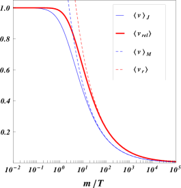
Figure 3: Mean values of relative velocity and single particle velocity given by Eqs. (100) and (101).

The average relative velocity (83) is useful in the relaxation time approximation of the Boltzmann equation [3], [14]

$$p\cdot\partial\texttt{f}=-\frac{E}{\tau_{\text{coll}}}(\texttt{f}-f^{\text{eq}}),$$ (98)

where $\tau_{\text{coll}}$ is a typical collision time. If the cross section does not vary strongly with the relative velocity, we can approximate $\langle\sigma v_{\text{rel}}\rangle_{\mathcal{P}}\simeq\sigma\langle v_{\text{rel}}\rangle_{\mathcal{P}}$ such that

$$\tau_{\text{coll}}\simeq\frac{1}{n^{\text{eq}}\sigma\langle v_{\text{rel}}\rangle}_{\mathcal{P}}.$$ (99)

For a gas composed of a single specie of mass $m$ the mean value (83) is given by the simple expression

$$\langle v_{\text{rel}}\rangle_{\mathcal{P}}=\frac{4}{x}\frac{K_{3}(2x)}{K^{2}_{2}(x)}\overset{\text{\tiny$x\gg 1$}}{\longrightarrow}\langle v_{r}\rangle=\sqrt{\frac{16}{\pi x}}.$$ (100)

This can be confronted for example with the complicated expression for $\langle\bar{v}\rangle$ calculated in [14] that in the ultrarelativistic limit tends to $4/5$, which evidently has no particular physical meaning. Another possibility is to use the mean value of the single particle velocity $\langle v\rangle_{J}=\int d^{3}\boldsymbol{p}f_{p}\frac{|\boldsymbol{p}|}{E}$, which is easily find to be

$$\langle v\rangle_{J}=2\frac{(1+x)}{x^{2}}\frac{e^{-x}}{K_{2}(x)}\overset{\text{\tiny$x\gg 1$}}{\longrightarrow}\langle v\rangle_{M}=\sqrt{\frac{8}{\pi x}}.$$ (101)

The averaged velocities and their nonrelativistic expression are shown in Figure 3. Note that $\langle v_{\text{rel}}\rangle$ and $\langle v\rangle_{J}$ tend to 1 in the ultrarelativistic limit $x\ll 1$ as required by relativity principle and that the relation $\langle v_{r}\rangle=\sqrt{2}\langle v\rangle_{M}$ is recovered in the nonrelativistic limit, $\langle v_{\text{rel}}\rangle/\langle v\rangle_{J}\sim\sqrt{2}+\mathcal{O}(x^{-1})$.

VII.4 Rate equation

The thermal averaged cross section appears in the integrated Boltzmann equation that gives the variation in time of the number density of a particle specie as a consequence of inelastic reactions and expansion of volume. The system departs from chemical equilibrium until it reaches a new stationary state or moves from a nonequilibrium state towards the equilibrium state.

An example of the former process is the departure from the equilibrium and freeze out of particle species in the early Universe.

An example of the latter is the equilibration of the hadronic system produced in high energy nucleus-nucleus collisions after the formation of the quark-gluon plasma.

Let us consider the case of the homogeneous and isotropic standard model of cosmology governed by the Friedman-Robertson-Walker metric with scale factor $a$ and Hubble parameter $H=\frac{1}{a}\frac{da}{dt}$. The distribution function depends only on $E$, $|\boldsymbol{p}|$, $t$ and the Boltzmann equation takes the form [7]

$$\frac{\partial\texttt{f}_{1}}{\partial t}-H\frac{|\boldsymbol{p}_{1}|}{E_{1}}\frac{\partial\texttt{f}_{1}}{\partial|\boldsymbol{p}_{1}|}=\int d^{3}\boldsymbol{p}_{2}k_{\text{r}}(\texttt{f}_{3}\texttt{f}_{4}-\texttt{f}_{1}\texttt{f}_{2})\sigma v_{\text{rel}},$$ (102)

where we used (97) to express the collision integral.

Assume that the product particles remain in equilibrium with zero chemical potential, then

$$\texttt{f}_{3}\texttt{f}_{4}=f^{\text{eq}}_{3}f^{\text{eq}}_{4}=f^{\text{eq}}_{1}f^{\text{eq}}_{2}=n^{\text{eq}}_{1}n^{\text{eq}}_{2}f_{p,1}f_{p,2},$$

where the second equality follows from energy conservation. Further assume that the nonequilibrium distribution of the colliding particles is proportional to the equilibrium one through the fugacity $\lambda=\exp(\mu/T)$ where $\mu$ is the chemical potential,

$$\texttt{f}_{1}\texttt{f}_{2}=\lambda_{1}\lambda_{2}f^{\text{eq}}_{1}f^{\text{eq}}_{2}=\lambda_{1}\lambda_{2}n^{\text{eq}}_{1}n^{\text{eq}}_{2}f_{p,1}f_{p,2}=n_{1}n_{2}f_{p,1}f_{p,2}.$$

Integrating in $\boldsymbol{p}_{1}$ the collision integral in (102) we have

$$(n^{\text{eq}}_{1}n^{\text{eq}}_{2}-n_{1}n_{2})\int d^{3}\boldsymbol{p}_{1}d^{3}\boldsymbol{p}_{2}k_{\text{r}}f_{p,1}f_{p,2}\sigma v_{\text{rel}},$$

where the integral is nothing but $\langle\sigma v_{\text{rel}}\rangle_{\mathcal{P}}$. The integral of the left-hand side of (102) gives $\frac{dn_{1}}{dt}+3Hn_{1}$, thus

$$\frac{1}{\nu_{1}}\frac{1}{a^{3}}\frac{d(n_{1}a^{3})}{dt}=\frac{1}{j_{12}}(n^{\text{eq}}_{1}n^{\text{eq}}_{2}-n_{1}n_{2})\langle\sigma v_{\text{rel}}\rangle_{\mathcal{P}}.$$ (103)

We have inserted the stoichiometric coefficient [11] on the left hand side and the statistical factor on the right hand side. In this way, when the species 1 and 2 are the same, the equation becomes

$$\frac{1}{a^{3}}\frac{d(na^{3})}{dt}=(n^{2}_{\text{eq}}-n^{2})\langle\sigma v_{\text{rel}}\rangle_{\mathcal{P}},$$ (104)

with $j_{12}=2$ cancelled by stoichiometric coefficient $\nu_{1}=2$. For an approach to rate equations based on nonequilibrium thermodynamics see [11].

VIII Final comments

The Lorentz invariant relative velocity given by formula (20) is practically unknown in quantum field theory and particle physics literature.

We have seen that thanks to (20), the formulation of the invariance flux, cross section and luminosity becomes simple and transparent. In this way the use of non physical velocity like the ‘Møller velocity’, and assumptions about reference frames and collinearity can be avoided. The cross sections for $2\to 2$ processes are easily expressed in the rest frame of a particle or in the center of momentum frame in terms the invariant relative velocity that also allows to obtain the correct nonrelativistic expansion.

Finally we have reviewed the statistical properties in a relativistic gas highlighting the role the probability density function of the relative velocity in the determination of reaction rates, Boltzmann equation and rate equations.

The relative velocity determines the metric and hyperbolic properties of the velocity space. This is not a mathematical curiosity but explains the peculiarities of the various ingredients that are necessary in formulating the theory of relativistic scattering.