Abstract

We study the performance of all-mode-averaging (AMA) when used in conjunction with a locally deflated SAP-preconditioned solver, determining how to optimize the local block sizes and number of deflation fields in order to minimize the computational cost for a given level of overall statistical accuracy. We find that AMA enables a reduction of the statistical error on nucleon charges by a factor of around two at the same cost when compared to the standard method. As a demonstration, we compute the axial, scalar and tensor charges of the nucleon in $N_{f}=2$ lattice QCD with non-perturbatively O($a$)-improved Wilson quarks, using O(10,000) measurements to pursue the signal out to source-sink separations of $t_{s}\sim 1.5$ fm. Our results suggest that the axial charge is suffering from a significant amount (5-10%) of excited-state contamination at source-sink separations of up to $t_{s}\sim 1.2$ fm, whereas the excited-state contamination in the scalar and tensor charges seems to be small.

1 Introduction

Recent developments in the field of numerical algorithms and computer hardware have made it possible to perform simulations of lattice QCD with dynamical light quarks at physical pion masses, enabling reliable first-principle determinations of hadronic and nuclear properties.

Indeed, with current technology the lattice computation of the light hadron spectrum, including not only the ground states, but also resonances, has become a routine task, which can be accomplished with great precision [1, 2, 3, 4, 5, 6]. On the other hand, attempts at achieving a similar precision for the prediction of nucleon structure observables from lattice QCD [7, 8, 9, 10, 11, 12, 13, 14, 15, 16] are confronted with a dilemma arising from the simultaneous problems of excited-state contamination at short, and deteriorating signal-to-noise ratio at large Euclidean times: while excited states are exponentially suppressed at large time separations, the signal-to-noise ratio likewise decays exponentially with time, and increases only with the square root of statistically independent measurements. As a result, controlling both statistical and systematic errors for nucleonic observables becomes difficult, in particular for structure observables, where both the time separation between the nucleon source and sink, and those between the source or sink and the operator insertion of interest, need to be made large to suppress excited-state contaminations.

It is therefore perhaps not surprising that the results for nucleon structure observables which have been obtained by different lattice collaborations currently show large discrepancies between the different groups (for details, cf. e.g. [17, 18, 19, 20] and references therein). The problem is particularly acute for the axial charge of the nucleon, which is both of fundamental importance for testing the limits of the Standard Model and well known experimentally, but for which lattice results differ amongst themselves by several standard deviations and show a discrepancy of about 10% from the experimental value when extrapolated to the physical point.

To address this problem, lattice studies of nucleon structure with high statistical accuracy at large Euclidean time separations are needed. Keeping the computational cost manageable requires efficient techniques of variance reduction. The present study aims to reduce the statistical noise by using the recently proposed technique of all-mode-averaging (AMA) [21, 22, 23]. AMA is able to achieve a significant reduction in statistical error at moderate cost by combining multiple cheap low-precision calculations of the quark propagator with an appropriate bias correction. This makes AMA particularly attractive for approaching the physical light quark mass, since the cost of computing quark propagators scales inversely proportional to the quark mass.

In this paper, we study the efficiency of AMA when combined with the highly efficient locally deflated SAP-preconditioned GCR solver. In an extension of our previous studies [13, 24, 25], we apply AMA to the calculation of the axial charge of the nucleon from three-point functions with large source-sink separations of around $1.5$ fm and above on large lattices satisfying $m_{\pi}L>4$ with $N_{\rm f}=2$ flavours of dynamical quarks. In addition, we also determine the scalar and tensor charges of the nucleon on the same configurations.

We find that for the axial charge as extracted from ratios of correlation functions, large source-sink separations are required to reliably suppress excited-state contaminations, which become visible only at high enough statistics, and that values close to the experimental one are obtained from the largest source-sink separations studied. The summation method [9, 13, 25] is able to extract the asymptotic behaviour already from moderate source-sink separations, but still profits greatly from having precise measurements at large separations.

This paper is organized as follows: In section 2, we explain the numerical methods, including how to properly define AMA when using the Schwartz alternating procedure (SAP) and local deflation with the GCR solver. We also define the ratios of three- and two-point functions that we use to extract the axial charge, scalar and tensor charge. In section 3, we study the performance of AMA and consider how to tune the solver parameters. In Section 4 and 5, we present a first analysis of the nucleon two-point function and three-point functions, respectively, using AMA with parameters tuned as presented in Section 3. In the last section, we summarize our results and discuss directions for further improvement and future study.

Table 1: Lattice parameters and gauge ensembles used in this analysis. The number $N_{\rm meas}$ of measurements is given by $N_{G}$ (see Table 3) multiplied by the number $N_{\rm conf}$ of configurations.

Label	Lattice($T\times L^{3}$)	$a$ [fm]	$m_{\pi}$ [MeV]	$t_{s}$ [fm]	$N_{\rm conf}$	$N_{\rm meas}$
A5	$64\times 32^{3}$	0.079	316	0.79	68	4,352
	(2.5 fm)3		($m_{\pi}L=4.0$)	0.95	74	4,672
				1.11	72	4,608
				1.26	71	4,544
				1.42	695	44,480
B6	$96\times 48^{3}$	0.079	268	0.79, 1.11	49	3,136
	(3.8 fm)3		($m_{\pi}L=5.0$)	1.26	281	17,984
				1.42	294	28,224
E5	$64\times 32^{3}$	0.063	456	0.82	559	35,776
	(2.0 fm)3		($m_{\pi}L=4.7$)	0.95	500	32,000
				1.13	489	31,296
				1.32	994	63,616
				1.51	1,605	102,720
F6	$96\times 48^{3}$	0.063	324	0.82	60	3,840
	(3.0 fm)3		($m_{\pi}L=5.0$)	0.95	150	9,600
				1.07	75	4,800
				1.32	254	16,256
				1.20, 1.51	299	19,136
F7	$96\times 48^{3}$	0.063	277	0.82, 0.95, 1.07	250	16,000
	(3.0 fm)3		($m_{\pi}L$=4.2)	1.20, 1.32	250	32,000
				1.51	250	64,000
G8	$128\times 64^{3}$	0.063	193	0.88	184	14,720
	(4.0 fm)3		($m_{\pi}L$=4.0)	1.07	112	19,040
				1.26	182	29,120
				1.51	344	44,032
N6	$96\times 48^{3}$	0.05	332	0.9	110	3,520
	(2.4 fm)3		($m_{\pi}L$=4.1)	1.1	888	28,416
				1.3, 1.5, 1.7	946	30,272

2 Numerical method

2.1 All-mode-averaging

The all-mode-averaging (AMA) estimator [21, 22, 23] for an observable $\mathcal{O}$ can be defined as

$$\mathcal{O}^{\rm AMA}=\mathcal{O}^{\rm(rest)}+\frac{1}{N_{G}}\sum_{g\in G}^{N_{G}}\mathcal{O}^{{\rm(appx)}\,g},$$ (1)

$$\mathcal{O}^{\rm(rest)}=\frac{1}{N_{\rm org}}\sum_{f\in G}^{N_{\rm org}}\Big{[}\mathcal{O}^{f}-\mathcal{O}^{{\rm(appx)}\,f}\Big{]},$$ (2)

where $\mathcal{O}^{\rm(appx)}$ denotes an approximate evaluation of $\mathcal{O}$ constructed by means of applying a “sloppy” inversion algorithm (a truncated solver with a precision of typically around $10^{-3}$) to the Dirac operator. The bias inherent in any truncated-solver method is corrected by the term $\mathcal{O}^{\rm(rest)}$. To ensure that the expectation value of $\mathcal{O}^{\rm AMA}$ is consistent with $\mathcal{O}$, both the sloppy and the exact evaluations of $\mathcal{O}$ are averaged over orbits $\mathcal{O}^{g}$ under some subset $G$ (of size $N_{G}$) of a symmetry group (such as translations) under which $\mathcal{O}$ transforms covariantly.

To improve the accuracy with which the bias correction $\mathcal{O}^{\rm(rest)}$ is estimated, it may also be averaged over an orbit $\mathcal{O}^{f}$ under a subset of size $N_{\rm org}\ll N_{G}$ of $G$. In this way, it becomes possible to reuse existing exact evaluations of $\mathcal{O}$ using different source positions to enhance the statistical accuracy without having to recalculate the exact evaluations.

The idea behind AMA is that, as long as $\mathcal{O}^{\rm(appx)}$ is an appropriate observable in the sense of having a strong correlation with the original observable $\mathcal{O}$, the statistical accuracy of $\mathcal{O}^{\rm AMA}$ evaluated on $N_{\rm conf}$ gauge configurations should be similar to that of $\mathcal{O}$ on $N_{\rm meas}=N_{G}\times N_{\rm conf}$ configurations, while the cost of evaluating $\mathcal{O}^{\rm(appx)}$ is much lower than that of evaluating $\mathcal{O}$. We should therefore expect to be able to achieve a much-increased statistical accuracy for the same effort, or conversely to have to pay only a reduced price for achieving a desired statistical error.

More specifically, the ratio between the standard deviations of $\mathcal{O}^{\rm AMA}$ and $\mathcal{O}$ is given by [23]

$$\sigma^{\rm AMA}/\sigma \simeq \sqrt{N_{G}^{-1}+2\Delta r+R},$$ (3)

$$\Delta r = \Big{(}\frac{1}{N_{\rm org}}-\frac{1}{N_{G}}\Big{)}\Big{(}1-\frac{1}{N_{\rm org}}\sum_{f\in G}^{N_{\rm org}}\frac{\langle\Delta\mathcal{O}^{f}\Delta\mathcal{O}^{{\rm(appx)}\,f}\rangle}{\sigma^{f}\sigma^{{\rm(appx)}\,f}}\Big{)},$$ (4)

$$\quad R = \frac{1}{N^{2}_{G}}\sum_{g,g^{\prime}\in G\atop g\not=g^{\prime}}^{N_{G}}\frac{\langle\Delta\mathcal{O}^{{\rm(appx)}\,g}\Delta\mathcal{O}^{{\rm(appx)}\,g^{\prime}}\rangle}{\sigma^{{\rm(appx)}\,g}\sigma^{{\rm(appx)}\,g^{\prime}}},$$ (5)

where $\Delta\mathcal{O}=\mathcal{O}-\langle\mathcal{O}\rangle$, and the standard deviation is given by $\sigma=\sqrt{\langle(\Delta\mathcal{O})^{2}\rangle}$.

The deviation from the ideal error-scaling behaviour $\sigma^{\rm AMA}\sim 1/\sqrt{N_{G}}$ is parameterised by two quantities: $\Delta r$ represents the degree of disagreement between $\mathcal{O}$ and $\mathcal{O}^{\rm(appx)}$ by tracking the amount by which the statistical fluctuations of $\mathcal{O}^{\rm(appx)}$ fail to track those of $\mathcal{O}$, while $R$ represents the amount by which using $N_{G}$ approximate measurements $\mathcal{O}^{\rm(appx)\,g}$ falls short of providing $N_{G}$ statistically independent measurements by tracking the degree to which the individual approximations $\mathcal{O}^{{\rm(appx)}\,g}$ are correlated amongst themselves. Note that we ignore the correlation between the exact measurements $\mathcal{O}^{f}$ because these are generally sufficiently few in number ($N_{\rm org}\ll N_{G}$) that it is always possible to choose the spatial separations between the sources large enough to render these correlations negligible.

To reduce the error on $\mathcal{O}^{\rm AMA}$ as far as possible, it is therefore desireable to achieve both $\Delta r\simeq 0$, indicating close tracking of the exact by the approximate measurements, and $R\simeq 0$, indicating nearly-independent measurements from different source locations. Achieving the latter primarily relies on a suitable choice of translation $g$ by large enough distances, whereas the former has to be achieved by ensuring that the parameters of the truncated solver used are suitably tuned.

2.2 AMA with a locally deflated SAP+GCR solver

So far, AMA has been mostly used with relatively inefficient solvers such as CG. It is therefore worthwhile to study whether the significant benefits reported in that context [26, 27] carry over to the case of a more efficient solver, such as Lüscher’s locally deflated SAP-preconditioned GCR solver [28, 29] used in the DD-HMC [30, 31, 32], MP-HMC [33], and openQCD [34, 35] codes.

Here we recall the basic features of the Schwarz Alternating Procedure (SAP), as discussed in refs. [28, 29]. When applied to the Dirac equation

$$D\psi=\eta\,,$$ (6)

the SAP is a “divide and conquer” strategy which starts by decomposing the lattice into two non-overlapping domains $\Omega$ and $\Omega^{*}$ consisting of blocks arranged in checkerboard fashion. The SAP then visits the blocks in turn, updating the field on each block to the solution of the Dirac equation with Dirichlet boundary conditions given by the field on the neighbouring blocks. Due to the checkerboard structure of the block decomposition, this can be done in parallel by simultaneously visiting first all black blocks and then all white blocks in parallel.

Denoting the points of $\Omega$ and $\Omega^{*}$ that have neighbours in $\Omega^{*}$ and $\Omega$, respectively, by $\partial\Omega^{*}$ and $\partial\Omega$, the Dirac operator can be decomposed into a sum

$$D=D_{\Omega}+D_{\Omega^{*}}+D_{\partial\Omega}+D_{\partial\Omega^{*}}\,,$$ (7)

where $D_{\Omega}$ acts only on the field at points $x\in\Omega$ with all terms involving fields in $\Omega^{*}$ set to zero, $D_{\partial\Omega}$ contains the terms through which points in $\Omega$ receive contributions from $\Omega^{*}$, and so forth. A complete cycle of the SAP can then be written as

$$\psi\mapsto(1-KD)\psi+K\eta$$ (8)

with the SAP kernel

$$K=D_{\Omega}^{-1}+D_{\Omega^{*}}^{-1}-D_{\Omega^{*}}^{-1}D_{\partial\Omega^{*}}D_{\Omega}^{-1}.$$ (9)

After $n_{\rm cy}$ SAP cycles starting from $\psi=0$, this corresponds to approximating the inverse of the Dirac operator by the polynomial

$$D^{-1}\approx M_{\rm SAP}=K\sum_{\nu=0}^{n_{\rm cy}-1}(1-DK)^{\nu}\,,$$ (10)

and this is used as a preconditioner by solving the right preconditioned equation

$$DM_{\rm SAP}\phi=\eta$$ (11)

using the generalised conjugate residual (GCR) algorithm and setting $\psi=M_{\rm SAP}\phi$ at the end [28]. The tunable parameters of the SAP preconditioner are therefore the block size and the number $n_{\rm cy}$ of SAP cycles.

To further accelerate the GCR solver, deflation may be used as a means of improving the condition number of the Dirac operator by separating the high and low eigenmodes for separate treatment. If the deflation fields $\{\phi_{k}\}_{k\leq N}$ span a subspace (the deflation subspace) containing good approximations to the low eigenmodes of the Dirac operator, an oblique projector to the orthogonal complement of the deflation subspace is given by

$$P_{L}=1-\sum_{k,l=1}^{N}D\phi_{k}\left(A^{-1}\right)_{kl}\phi_{l}^{\dagger}\,,$$ (12)

where

$$A_{kl}=(\phi_{k},D\phi_{l})$$ (13)

is called the little Dirac operator. The Dirac equation can then be split into a low-mode and a high-mode part by left-projecting with $1-P_{L}$ and $P_{L}$, respectively. The low-mode part can be solved in terms of the little Dirac operator, so that the solution is given by

$$\psi=\chi+\sum_{k,l=1}^{N}\phi_{k}\left(A^{-1}\right)_{kl}(\phi_{l},\eta)\,,$$ (14)

where the high-mode part $\chi=P_{R}\psi$ satisfies

$$P_{L}D\chi=P_{L}\eta\,,~{}~{}~{}~{}(1-P_{R})\chi=0$$ (15)

with $P_{L}D=DP_{R}$ [29].

Combining the block-decomposition approach with deflation leads to the construction of a deflation subspace of dimension $N=N_{s}N_{b}$, where $N_{b}$ is the number of blocks, and each deflation field has support only on a single block. In practice, such deflation fields are obtained by restricting a set of $N_{s}$ global deflation fields to each block and orthonormalising the resulting fields using the Gram-Schmidt procedure. To ensure that the deflation space approximates the low eigenspaces of the Dirac operator efficiently, the global fields should ideally be good approximations to the low modes. Such approximations can be obtained using a few rounds of the inverse iteration $\phi_{l}\mapsto D^{-1}\phi_{l}$ starting from random fields. Since only approximate low modes are needed, the exact inverse of the Dirac operator is not required, and the SAP approximation $M_{\rm SAP}$ can be used instead [29]. Note that by using the block decomposition, we effectively are able to obtain $N$ deflation vectors for the price of computing only $N_{s}\ll N$ approximate eigenmodes. The tunable parameters of the deflation procedure are then the block size and the number $N_{s}$ of global deflation fields.

For a more efficient implementation, mixed-precision calculations can be used; since the SAP preconditioner needs not be very precise, single-precision arithmetic suffices in this case. In the GCR algorithm, likewise, some operations can be carried out in single precision [28].

In line with the setup used in the generation of the Monte Carlo ensembles, we keep $n_{\rm cy}=5$ fixed in our setup. The remaining algorithmic parameters that control the quality of the sloppy solves, as measured by $\Delta r$ in Eq.(4) are then the iteration number $N_{\rm iter}$ of the GCR algorithm, the block size (which for simplicity we take to be the same for the SAP preconditioner and the deflation procedure), and the number $N_{s}$ of global deflation fields. Tuning these parameters requires one to make a trade-off between the quality of the AMA approximation and the gain in performance from using the sloppy solver. In the case of the iteration number this is obvious, while in the case of the deflation parameters the trade-off comes from the increase of the size (and hence condition number) of the little Dirac operator with $N_{s}$ and the number of blocks. We will study the dependence of the overall runtime on these parameters in section 3 below.

A notable feature of the block-decomposition technique is that for translations within the same block the translation invariance of the approximate solution $\mathcal{O}^{\rm(appx)}$ may be broken due to the limited precision of the sloppy solver in conjunction with the Dirichlet boundary conditions imposed in each SAP cycle. To preserve the translational invariance of $\mathcal{O}^{\rm(appx)\,g}$ under all transformations $g\in G$, we use only shifts that map the domains $\Omega$ and $\Omega^{*}$ onto themselves. As $M_{\rm SAP}$ is invariant under such translations, these shifts are not affected by broken translation invariance.

2.3 Computation of nucleon charges

In this paper we concentrate on the application of AMA to computating the axial ($g_{A}$), scalar ($g_{S}$) and tensor ($g_{T}$) charges of the nucleon in lattice QCD. These observables can be extracted from suitably renormalised ratios of two- and three-point functions involving the operators of the axial current $A_{\mu}=\bar{\psi}\gamma_{\mu}\gamma_{5}\psi$, scalar density $S=\bar{\psi}\psi$, and tensor current $T_{\mu\nu}=\bar{\psi}\sigma_{\mu\nu}\psi$, respectively.

For the nucleon, we use the interpolating field

$$N_{\alpha}=\varepsilon^{abc}(u^{a}C\gamma_{5}d^{b})u_{\alpha}^{c},$$ (16)

where $C$ is the charge conjugate matrix, $\alpha$ is the Dirac spinor index, and $a,b,c$ are the color indices of the quark fields. (In the following we will omit the spin indices from our notation).

In order to increase the overlap between the nucleon ground state and the state created by applying the interpolating operator to the vacuum, we apply Gaussian smearing [9] (with APE-smeared [36] gauge links in the Laplacian) at both source and sink. The smearing parameters used are the same as in [25, 37].

Using the spin-projection matrices $P^{+}=\frac{1}{2}(1+\gamma_{0})$ and $P_{53}^{+}=P_{+}\gamma_{5}\gamma_{3}$, we evaluate the charges of the nucleon through computing the ratios of three- and two-point functions given

$$R_{A}^{\rm bare}(t,t_{s}) = \frac{{\rm tr}\Big{[}P_{53}^{+}\langle N(t_{s})A_{3}(t)\bar{N}(0)\rangle\Big{]}}{{\rm tr}\Big{[}P^{+}\langle N(t_{s})\bar{N}(0)\rangle\Big{]}},$$ (17)

$$R_{S}^{\rm bare}(t,t_{s}) = \frac{{\rm tr}\Big{[}P^{+}\langle N(t_{s})S(t)\bar{N}(0)\rangle\Big{]}}{{\rm tr}\Big{[}P^{+}\langle N(t_{s})\bar{N}(0)\rangle\Big{]}},$$ (18)

$$R_{T}^{\rm bare}(t,t_{s}) = \frac{{\rm tr}\Big{[}P_{53}^{+}\langle N(t_{s})T_{12}(t)\bar{N}(0)\rangle\Big{]}}{{\rm tr}\Big{[}P^{+}\langle N(t_{s})\bar{N}(0)\rangle\Big{]}},$$ (19)

which yield the (bare) charges $g_{A}^{\rm bare}$, $g_{S}^{\rm bare}$, and $g_{T}^{\rm bare}$, respectively, at asymptotically large time separations,

$$\lim_{t_{s},t_{s}-t\rightarrow\infty}R_{\mathcal{O}}^{\rm bare}=g_{\mathcal{O}}^{\rm bare}.$$ (20)

At finite time separations the ratio $R_{\mathcal{O}}^{\rm bare}$ differs from its asymptotic value $g_{\mathcal{O}}^{\rm bare}$ by time-dependent contributions from excited states with the same quantum numbers as the ground state. We will discuss in section 5 how to best suppress these contributions, and how the use of AMA can help to obtain a good signal even at relatively large time separations.

To further improve the statistical quality of the signal for the ratio $R_{\mathcal{O}}^{\rm bare}$, we average over the forward- and backward-propagating nucleon, constructing the ratio separately for each direction in order to take optimal advantage of correlations between the two- and three-point functions. Obtaining the three-point function for both directions requires the computation of sequential propagators with sink positions at both $t_{s}$ and $T-t_{s}$, whereas the two-point function for both directions can be obtained from a single inversion by using opposite parity projections for the forward and backward directions.

We note that, since the charges are defined at zero momentum transfer and we use the spatial components of the axial vector and tensor currents, no additional operators are needed to realise O($a$) improvement. To obtain the renormalised charges $g_{\mathcal{O}}=Z_{\mathcal{O}}g_{\mathcal{O}}^{\rm bare}$, we therefore only need to include the appropriate renormalisation constants, which should ideally be chosen such that O($a$) improvement is realised. We use the non-perturbative determination of $Z_{A}$ computed in the Schrödinger functional [38] together with the perturbative mass correction $b_{A}$ from [39], while for $Z_{S}$ and $Z_{T}$ we take the non-perturbative evaluations in the $\rm\overline{MS}$ scheme at a renormalisation scale of $\mu=2$ GeV using the RI-MOM scheme [15]. Since the values of the bare coupling used in [15] are slightly different from the ones used by us, we determine the values of $Z_{S}$ and $Z_{T}$ to use by linear interpolation and extrapolation in $1/\beta$, ignoring the unknown mass correction terms. In summary, our renormalised ratios are related to the bare ones by

$$R_{A}(t,t_{s}) =Z_{A}(1+b_{A}m_{q}a)R_{A}^{\rm bare}(t,t_{s})\,,$$ (21)

$$R_{S}(t,t_{s};\mu) =Z_{S}(\mu)R_{S}^{\rm bare}(t,t_{s})\,,$$ (22)

$$R_{T}(t,t_{s};\mu) =Z_{T}(\mu)R_{T}^{\rm bare}(t,t_{s})\,.$$ (23)

Table 2 shows the values of the renormalisation constants used in this paper.

Table 2: Renormalisation factors for the axial current, $Z_{A}^{\rm eff}=Z_{A}(1+b_{A}am_{q})$, from [38, 39], and for the scalar operator, $Z_{S}^{\rm\overline{MS}}(2~{}\rm{GeV})$, and the tensor operator, $Z_{S}^{\rm\overline{MS}}(2~{}\rm{GeV})$, from [15]. A perturbative error of the same order as the one-loop contribution to $b_{A}$ is included in $Z_{A}^{\rm eff}$.

label	$Z_{A}^{\rm eff}$	$Z_{S}^{\rm\overline{MS}}$	$Z_{T}^{\rm\overline{MS}}$
A5	0.7785(83)	0.6196(54)	0.8356(15)
B6	0.7777(76)	0.6196(54)	0.8356(15)
E5	0.7866(83)	0.6152(32)	0.8540(91)
F6	0.7842(59)	0.6152(32)	0.8540(91)
F7	0.7835(51)	0.6152(32)	0.8540(91)
G8	0.7825(42)	0.6152(32)	0.8540(91)
N6	0.8022(91)	0.6082(31)	0.8886(95)

3 Tests and performance of AMA

In order to achieve the greatest possible gain in statistical accuracy for fixed computational effort, we need to appropriately tune the parameters of the sloppy solver.

3.1 Covariance test

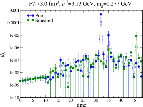
Figure 1: The covariance violation $|\delta_{c}|$ defined in (24) for the nucleon two-point function as a function of source-sink separation as measured on one F7 configuration ($96\times 48^{3}$ lattice, $m_{\pi}=0.277$ GeV). The different colors indicate the results obtained using smeared (green squares) and point (blue circles) sources and sinks, respectively.

Before discussing how to tune the parameters of AMA for use with the deflated SAP-preconditioned GCR solver, we first need to check that the covariant symmetry of the approximation is preserved in the presence of the domain decomposition underlying the SAP preconditioner.

The amount by which the assumed covariance is violated can be parameterized by [23]

$$\delta_{c}=(\mathcal{O}^{{\rm(appx)}\,g}[U^{\bar{g}}]-\mathcal{O}^{(\rm appx)}[U])/\mathcal{O}^{(\rm appx)}[U],$$ (24)

i.e. the relative difference between evaluating the original observable on the original gauge field and evaluating the approximation based on the transformation $g$ on the appropriately transformed gauge field; if covariance were exact, we would find $\delta_{c}=0$.

For a numerical test, we use the F7 ensemble from Table 1, choosing a domain size of $6^{4}$ for the SAP preconditioner. In line with the arguments laid out in Section 2.2, shift vectors need be such that each of the SAP subdomains is mapped onto itself; we therefore choose the shifted source location to be $g=(6,6,0,0)$, with the corresponding shift of the gauge field given by $\bar{g}=(-6,-6,0,0)$. Since the point of this comparison is to check that the effects of the block decomposition in the SAP are under control, we did not use deflation for this test. For the approximation, we therefore had to choose a fixed iteration count of $N_{\rm iter}=30$ for the GCR algorithm, which in our example corresponds to a residual norm of order $10^{-2}$. The resulting covariance violation $|\delta_{c}|$ for the nucleon two-point function as a function of the source-sink separation is shown in Figure 1. At large time separations $t\gtrsim 30a$, the accumulation of round-off errors in the approximation leads to a non-negligible covariance violation $|\delta_{c}|\sim 10^{-5}-10^{-3}$ (which however is still less than the statistical errors in this time region). On the other hand, the covariance assumption is well-justified in the typical signal region $t\lesssim 25a$, where $|\delta_{c}|\lesssim 10^{-6}$. We may therefore conclude that with this set of parameters, the systematic error arising from violating the covariance assumption is negligible for practical purposes.

3.2 Correlation between original and approximation

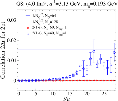
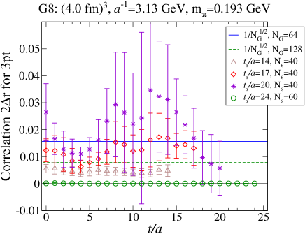
Figure 2: The correlation mismatch $2\Delta r$ on the G8 ensemble ($128\times 64^{3}$ lattice, $m_{\pi}=0.193$ GeV) for the nucleon two-point function (left) and the axial-vector nucleon three-point function (right), as a function of the source-sink separation $t_{s}$ and operator insertion time $t$. The straight lines indicate the level of the statistical error reduction achievable with AMA in the case of mutually perfectly decorrelated approximations that are each perfectly correlated with the original observable.

Given that the statistical error of the AMA result depends crucially on the discrepancy $\Delta r$ between the fluctuations of the original observable and its approximate evaluation, our tuning of the solver parameters will have to be guided by considering the parameter dependence of $\Delta r$.

The left panel of Figure 2 shows $2\Delta r$ for the nucleon two-point function as a function of source-sink separation using both $N_{s}=40$ and $N_{s}=60$ deflation vectors. For $N_{s}=40$, an increase in $\Delta r$ can be seen at larger time separations $15\leq t/a\leq 25$, where it becomes large enough to no longer be negligible compared to $1/N_{G}$ for $N_{G}=128$. For $N_{s}=60$, on the other hand, we find $\Delta r\lesssim 10^{-3}$ all the way out to $t/a=25$ (corresponding to a separation of $\sim 1.5$ fm). The optimal choice of the parameters for the approximation therefore will in general depend on the maximal time separation one is interested in.

The right panel of Figure 2 shows $\Delta r$ for the three-point function appearing in the numerator of the ratio $R_{A}$ as a function of the operator insertion time $t$ for a range of different source-sink separations $t_{s}$. For $N_{s}=40$, $\Delta r$ is seen to increase with $t_{s}$, becoming comparable to $1/N_{G}$ for $N_{G}=128$ at $t_{s}/a=20$. Since $\Delta r$ can be reduced by increasing $N_{\rm org}$ as per Eq. (4), we use $N_{\rm org}>1$ for $t_{s}/a=20$. For $N_{s}=60$, we see that $\Delta r$ is sufficiently reduced to be negligible even at $t_{s}/a=24$, albeit at the expense of a 1.6-fold increase in computing time (cf. Figure 3), indicating that the trade-off between computational cost and achievable statistical accuracy is a crucial consideration in tuning the parameters of the approximation used in AMA.

3.3 Performance of AMA for different approximation parameters

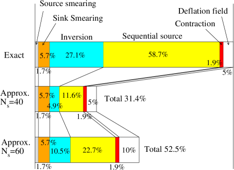
Figure 3: A comparison of the computational cost between the exact (using $N_{s}=40$ deflation vectors) and two approximate evaluations (using $N_{s}=40$ and $N_{s}=60$, respectively) of the axial charge of the nucleon on the G8 ensemble. All percentages given are relative to the total time for the exact evaluation.

In Figure 3, we show a comparison of the overall performance of two different approximations (using $N_{s}=40$ and $N_{s}=60$ deflation vectors, respectively) relative to the exact evaluation (with $N_{s}=40$ deflation vectors), using the G8 ensemble as a test case. For the approximation with $N_{s}=40$, the time required for inverting the Dirac operator is reduced by a factor of 5, whereas for $N_{s}=60$, the reduction is only by a factor of 3 due to the larger size of the “little” Dirac operator (13) in Eq. (14). Taking into account the fact that generating a larger number of deflation fields is also more costly, and including the fixed costs of source and sink smearing and contractions, the total time for an approximate evaluation using $N_{s}=40$ is about 30% of the exact calculation, whereas for $N_{s}=60$ it is about 50%.

3.4 Error scaling and computational cost

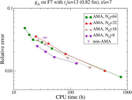
Figure 4: The relative error of the axial charge measured on the F7 ensemble using $t_{s}/a=13$, $t/a=7$ plotted against the total CPU time used. The different symbols and colours denote different values for $N_{G}$, where the error scaling for each is explored using different numbers of gauge configurations. In the case of the non-AMA evaluation, the complete gauge ensemble is used with a single source position for the exact evaluation.

Finally, we consider how the overall statistical error scales as a function of the total CPU time used when varying the total number of measurements by varying $N_{G}$, $N_{\rm conf}$, or both.

Figure 4 shows the relative error of the ratio $R_{A}(t,t_{s})$ from Eq. (21), as measured on the F7 ensemble using $t_{s}/a=13$ and $t/a=7$, plotted against the total CPU time used for AMA with $N_{G}=8$, $16$, $32$, and $64$, with different numbers of configurations used. The relative error and CPU time required when not using AMA and performing a single exact evaluation on each configuration instead is also shown for comparison.

Since increasing $N_{G}$ leads to an increase in the correlation $R$ between the different approximations (because the source positions $g$ will have to be taken closer together when using more approximate solves), the error scaling between different values of $N_{G}$ is not perfect. In our test case, using $N_{G}=8$ requires about half the computational cost at the same relative error as the larger values of $N_{G}$ considered, whereas the larger $N_{G}$ values exhibited roughly identical error scaling.

Comparing AMA to the conventional method, a reduction in error by a factor of about $1.5-3$ can be achieved at constant computational cost by using AMA. This is one of the main findings of this paper concerning the performance and effectiveness of AMA in conjunction with highly efficient solvers.

3.5 Tuning of AMA parameters

Table 3: AMA tuning parameters for each gauge ensemble.

Label	Domain size	$N_{s}$	$N_{G}$	$N_{\rm iter}$	$N_{\rm org}$	$t_{s}$ [fm]
	(T$\times$ X$\times$ Y$\times$ Z)			(2pt, 3pt)
A5	4$\times$4$\times$4$\times$4	30	64	(3,3)	1	0.79, 0.95, 1.11
						1.26, 1.42
B6	6$\times$6$\times$6$\times$6	40	64	(4,3)	1	0.79, 1.11, 1.26
		40	96	(3,3)	1	1.42
E5	4$\times$4$\times$8$\times$8	30	64	(3,3)	1	0.82, 0.95,
						1.13, 1.32
		30(994 cfgs.)	64	(3,3)	5	1.51
		40(661 cfgs.)
F6	6$\times$6$\times$6$\times$6	30	64	(4,3)	1	0.82, 0.95, 1.07
						1.20, 1.32
		40	64	(4,3)	1	1.51
F7	6$\times$6$\times$6$\times$6	30	64	(4,3)	1	0.82, 0.95, 1.07
		30	64	(4,3)	4	1.2, 1.32
		40	64
		30	192	(4,3)	15	1.51
		40	64
G8	8$\times$8$\times$8$\times$4	40	80	(4,3)	1	0.88
		40	170	(4,3)	1	1.07
		40(101 cfgs.)	160	(4,3)	5	1.26
		50(81 cfgs.)	160
		60	128	(4,3)	1	1.51
N6	6$\times$6$\times$6$\times$6	30	64	(4,3)	1	0.9, 1.1, 1.3
						1.5, 1.7

For the remaining calculations, we have tuned the parameters of the deflated SAP-preconditioned GCR solver so as to achieve the maximum reduction in computational cost while keeping $\Delta r$ sufficiently suppressed to enable good error scaling. Table 3 shows the resulting tuned parameter values.

We use fixed numbers $N_{\rm iter}$ of GCR iterations for the point-to-all propagator and the sequential propagator, as shown in Table 3; using a sloppier propagator between the sink and operator insertion point does not lead to an increase of $\Delta r$, and thus enables us to reduce the computational cost for the three-point function. We note that the iteration count of $N_{\rm iter}=3$ corresponds to a similar residual as $N_{\rm iter}=30$ in the undeflated test of section 3.1.

4 AMA study of excited-state contamination in nucleon two-point functions

The nucleon two-point correlation function may be approximated as

$$C_{N}(t)\simeq Z_{N}e^{-m_{N}t}+Z_{N^{\prime}}e^{-m_{N^{\prime}}t}+\cdots,$$ (25)

with masses $m_{N}$ and $m_{N^{\prime}}$ and overlap factors $Z_{N}$ and $Z_{N^{\prime}}$, for the ground state and first excited state respectively. In order to study the nucleon mass, we utilised single- and double-exponential fits to the correlation function eq. (25), of the form

$$C_{N}(t) = Ae^{-mt},$$ (26)

$$C_{N}(t) = Ae^{-mt}+Be^{-(m+\Delta)t}.$$ (27)

For the fitting, we used a $\chi$-squared minimisation and found that the nucleon mass could be determined reliably using a single-exponential fit performed in the interval 1.0 fm$~{}<t<~{}$1.5 fm (confirmed by the double-exponential fits), whereas in order to incorporate the excited states fitted in the double-exponential fits, an earlier fitting interval was required, starting at $t\simeq 0.5$ fm. This is highlighted by the plots in Figure 5, where the effective mass

$$m^{\rm eff}_{N}(t)=\ln\frac{C_{N}(t)}{C_{N}(t+1)},$$ (28)

is used to monitor the region of ground state dominance and of excited-state contamination. It also indicates the effectiveness of the exponential fits.

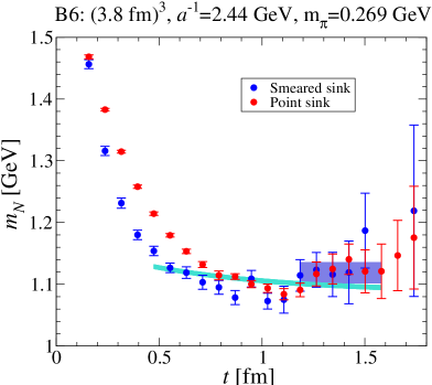
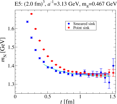
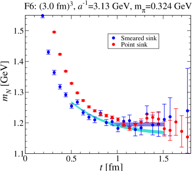
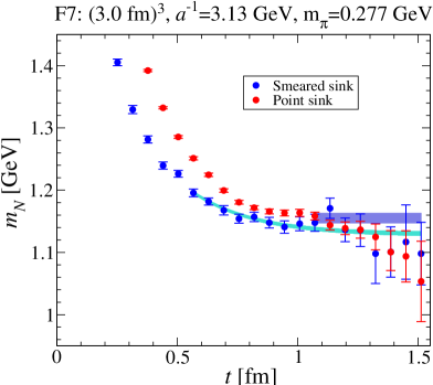
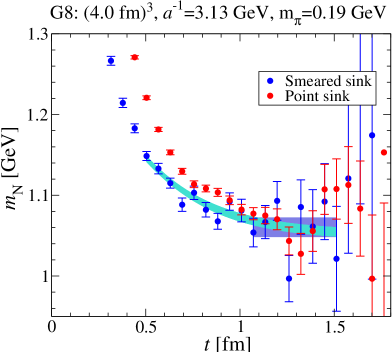
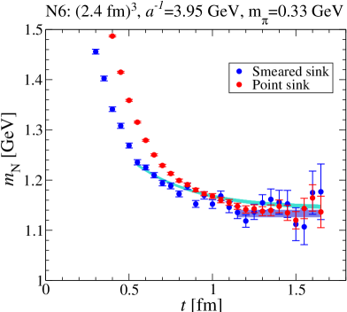
Figure 5: Effective mass plots of the nucleon for six gauge ensembles. The ensemble parameters are indicated in the plots. The two colours indicate the different nucleon sink operators. The blue and cyan bands indicate the results and errors from single- and double-exponential fits to the correlator.

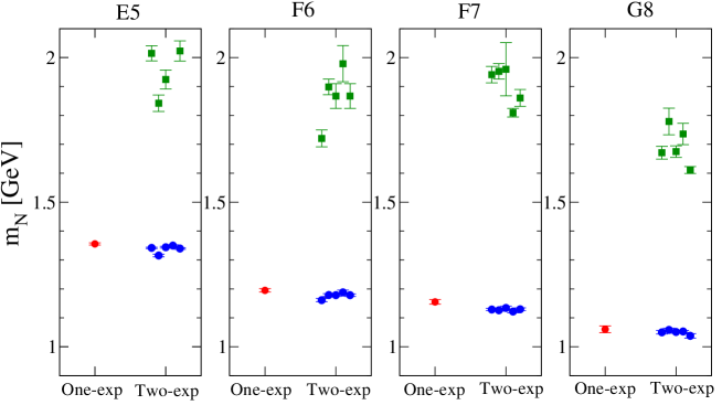
Figure 6: Results for single- (red points) and double-exponential fits to the nucleon two-point function for the $\beta=5.3$ gauge ensembles. For the double-exponential fits, the blue and green points indicate the ground and excited state masses respectively, for a number of different fitting intervals (indicated in Table 4).

Table 4: Results for single- and double-exponential fits to the nucleon two-point function on each gauge ensemble. The nucleon mass, $\chi^{2}$/dof and fitting intervals (in lattice units) are given. To determine the masses, the largest set of measurements available in Table 1 for each ensemble was used (i.e. for ensemble E5 the measurement set where $N_{\mathrm{meas}}=102,720$ was used)

	Single-exp.	Double-exp.					Ref. [40]
A5	[15,20]	[6,20]	[5,20]	[7,20]	[6,19]	[6,21]	[10,25]
$am_{N}$	0.465(6)	0.437(1)	0.444(2)	0.444(2)	0.437(2)	0.449(1)	0.468(7)
$\chi^{2}$/dof	0.8	4.6	1.54	2.9	2.6	4.8	0.9
B6	[15,20]	[6,20]	[5,20]	[7,20]	[6,19]	[6,21]	[8,20]
$am_{N}$	0.448(7)	0.436(2)	0.444(2)	0.424(1)	0.433(4)	0.434(2)	0.444(5)
$\chi^{2}$/dof	0.4	3.8	13.2	2.3	1.0	1.2	1.3
E5	[15,23]	[7,23]	[6,23]	[8,23]	[7,22]	[7,24]	[11,25]
$am_{N}$	0.433(1)	0.429(1)	0.421(1)	0.430(1)	0.432(1)	0.429(2)	0.441(4)
$\chi^{2}$/dof	0.5	2.5	5.3	1.6	0.6	2.2	1.1
F6	[15,24]	[8,24]	[7,24]	[9,24]	[8,23]	[8,25]	[11,25]
$am_{N}$	0.382(2)	0.370(2)	0.376(1)	0.376(1)	0.379(3)	0.376(1)	0.382(4)
$\chi^{2}$/dof	0.6	1.9	1.5	1.6	1.6	1.6	1.0
F7	[17,24]	[9,24]	[8,24]	[10,24]	[9,23]	[9,25]	[11,25]
$am_{N}$	0.369(3)	0.361(1)	0.360(1)	0.363(2)	0.359(2)	0.361(2)	0.367(5)
$\chi^{2}$/dof	0.9	1.1	1.3	1.1	1.5	1.2	0.58
G8	[17,24]	[8,24]	[7,24]	[9,24]	[8,23]	[8,25]	[11,24]
$am_{N}$	0.338(4)	0.335(2)	0.338(2)	0.336(1)	0.336(1)	0.331(2)	0.352(6)
$\chi^{2}$/dof	1.3	1.5	1.8	0.9	1.6	1.6	1.4
N6	[23,33]	[11,33]	[10,33]	[12,33]	[11,32]	[11,34]	[15,30]
$am_{N}$	0.288(2)	0.290(1)	0.285(2)	0.290(7)	0.293(1)	0.290(1)	0.297(3)
$\chi^{2}$/dof	1.3	2.7	2.2	3.3	2.7	2.6	0.69

The results for the single- and double-exponential fits to the correlation function for each of the ensembles are given in Table 4, four of which are displayed in Figure 6. For the subsequent analysis, we took the single-exponential results for the extracted ground state nucleon mass. Whilst we see a small discrepancy for this value obtained from double-exponential fits, we find that, overall, the double-exponential fits largely confirm the single-exponential fits to be in the ground-state region. The observed discrepancy within the double-exponential fits (dependent on the fitting interval) is, in part, due to the contamination by higher excited states, which are not accounted for by the double-exponential fitting ansatz Eq. (27).

For reference, we also show our previous results from [40] in Table 4 and note that for three ensembles (labelled E5, N6 and G8) we observe a discrepancy between the new single-exponential results and our previous results. This is due to the increased statistics on these ensembles, which allows us to better identify the contamination from excited states and hence provide a revised determination of the nucleon mass at later fitting intervals.

5 AMA study of excited-state contamination in nucleon three-point functions

The ratios $R_{A}$, $R_{S}$ and $R_{T}$,

$$R_{\mathcal{O}}(t,t_{s})=g_{\mathcal{O}}+c_{\mathcal{O}}\big{(}e^{-\Delta t_{s}}+e^{-\Delta(t_{s}-t)}\big{)}+O(e^{-\Delta^{\prime}(t_{s}-t)}),$$ (29)

with the target observable $g_{\mathcal{O}}$, mass difference $\Delta$ and unknown coefficient $c_{\mathcal{O}}$ suffer excited state contamination at finite $t$ and $t_{s}$. For the subsequent analysis, we used both the plateau method that assumes ground state dominance around the middle of each $t_{s}$ dataset and the summation method [9, 13, 25].

5.1 Axial charge

5.1.1 Plateau method

In Figure 7 we show $g_{A}$ obtained from plateau fits to the middle 4 points (3 for N6) of the ratio $R_{A}(t,t_{s})$, for each $t_{s}$. The ratio $R_{A}(t,t_{s})$ typically resembles the example shown in Figure 8 (right panel) for the F7 ensemble. This demonstrates a clear tendency for the plateau results to approach the experimental value from below as $t_{s}$ is increased and indicates a significant contribution from the excited states in Eq. (29), which is especially pronounced for N6 (small lattice spacing) and G8 (small pion mass). The excited state contamination is significant at $t_{s}=1$ fm, which supports our previous findings [25] that the plateau method still suffers from substantial excited state contamination at $t_{s}=1.3$ fm and that 1.5 fm or more may be required. The plateau fit results at each $t_{s}$ for ensemble F7 are given in Table 5, for which the extracted $g_{A}$ results can be clearly seen to approach the experimental value as the source-sink separation is increased. The results for the largest $t_{s}$ on each ensemble are summarised in Table 6.

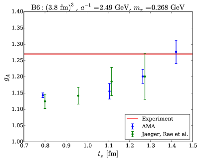
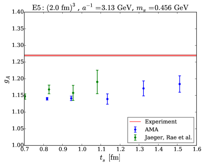
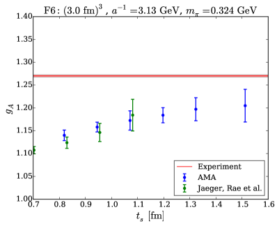
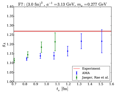
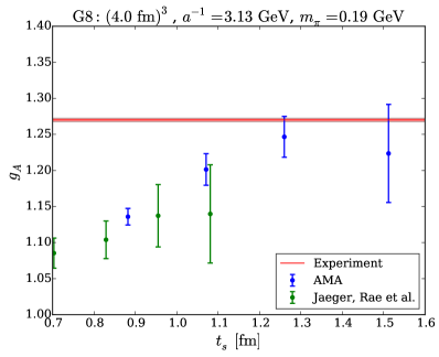
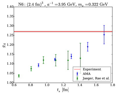
Figure 7: $g_{A}$ as a function of $t_{s}$ from plateau fits. Green symbols denote our previous results [25] on the same configurations but without AMA. These have been rescaled to account for the updated renormalisation factors in Table 2.

Table 5: $g_{A}$ on the F7 gauge ensemble, $m_{\pi}=277$ MeV. Using the plateau method for each source-sink separation and the summation method result.

$t_{s}/a$	$t_{s}$ [fm]	$g_{A}$
13	0.82	1.123(09)
15	0.95	1.139(13)
17	1.07	1.140(18)
19	1.20	1.164(26)
21	1.32	1.217(40)
24	1.51	1.217(61)
Sum (all $t_{s}$)		1.218(48)
Sum ($t_{s}>0.9$ fm)		1.244(82)
Exp.		1.272(02)

Table 6: $g_{A}$ determined using the plateau method for the largest source-sink separation, $t_{s}^{\mathrm{max}}$, for each gauge ensemble. The approximate pion and nucleon masses are given for reference.

Label	$m_{\pi}$ [MeV]	$m_{N}$ [MeV]	$g_{A}$ plateau $t_{s}^{\mathrm{max}}$
A5	316	1160	1.255(35)
B6	268	1120	1.277(36)
E5	456	1350	1.184(25)
F6	324	1190	1.205(36)
F7	277	1150	1.217(61)
G8	190	1090	1.224(68)
N6	332	1130	1.254(49)
Exp.	139	939	1.272(02)

5.1.2 Summation method

Performing the summation $S_{\mathcal{O}}(t_{s})$ parametrically reduces the excited state contamination,

$$S_{\mathcal{O}}(t_{s})\equiv\sum_{t=1}^{t_{s}-1}R_{\mathcal{O}}(t,t_{s})=d_{1}+\big{(}g_{\mathcal{O}}+O(e^{-\Delta t_{s}})\big{)}t_{s},$$ (30)

and through determining $S_{\mathcal{O}}(t_{s})$ for a number of $t_{s}$, the target observable may be obtained from the slope of a linear fit.

The $t_{s}$ dependence of the summed data points, including the linear fits, for the F7 ensemble are shown in Figure 8 and the results are summarised in Table 5. To check the dependence of the fit on the smaller $t_{s}$ points, the linear fits were performed for two intervals. One used all the $t_{s}$ points and the other used only the points where $t_{s}>0.9$ fm. We observe no statistically significant discrepancy between the two fits and therefore we quote the statistically more accurate result that incorporates all $t_{s}$ points.

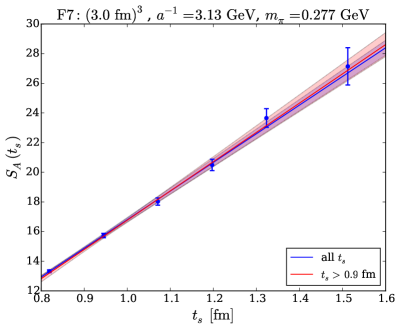
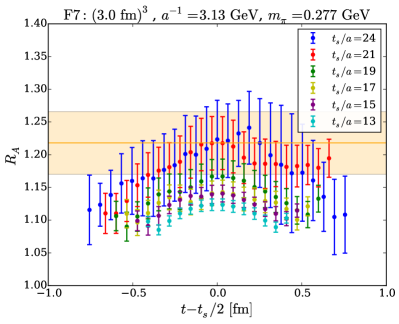
Figure 8: Left panel: $S_{A}$ as a function of $t_{s}$ on the F7 gauge ensemble. The solid lines are linear fits to all $t_{s}$ points (blue) and only for points where $t_{s}>0.9$ fm (red). The bands indicate the statistical error of the respective fit. Right panel: $R_{A}(t,t_{s})$ for the nucleon axial charge as a function of $t-t_{s}/2$ with the summation result for all $t_{s}$ overlaid.

5.2 Scalar and tensor charge

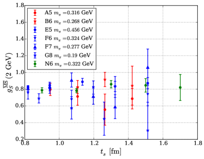
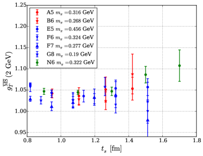
Figure 9: Renormalised scalar charge $g_{S}$ (left panel) and $g_{T}$ (right panel) as a function of $t_{s}$ obtained from plateau fits.

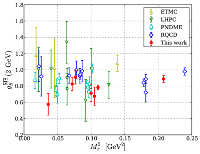
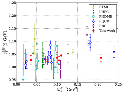
Figure 10: Left panel: results for $g_{S}$ from ETMC [41, 42], LHPC [43], PNDME [18, 44], and RQCD [15] (open symbols) compared to this work (filled symbols) as a function of $m_{\pi}^{2}$; right panel: results for $g_{T}$ from ETMC [45, 42], LHPC [43], PNDME [18, 44], RQCD [15], and RBC/UKQCD [46] (open symbols) compared to this work (filled symbols) as a function of $m_{\pi}^{2}$. All results are quoted using a renormalisation scale of 2 GeV.

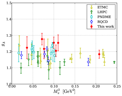
Figure 11: Results for $g_{A}$ from ETMC [47, 48, 42], LHPC [49, 50], PNDME [18, 44], and RQCD [15] (open symbols) compared to this work (filled symbols, plateau method only) as a function of $m_{\pi}^{2}$.

Figure 9 shows the renormalised scalar charge $g_{S}$ and tensor charge $g_{T}$, extracted from the ratio of the two- and three-point functions defined in Eq. (18) and Eq. (19) and obtained from plateau fits (to the same intervals as for $g_{A}$). In contrast to $g_{A}$, the dependence on $t_{s}$ is very mild with no evidence of excited state contaminations, even for a fine lattice spacing (N6) or for a light pion mass (G8). This echoes the behaviour seen by other groups, such as [18, 15]. In Figure 10 we show a comparison of lattice results for these quantities, where we use our plateau fit results for $t_{s}\sim 1.1$ fm, which we believe to be reasonable due the absence of excited state behaviour in these quantities, as seen in Figure 9. A similar comparison for the case of $g_{A}$ is shown in Figure 11, but we caution that the results obtained from the plateau method shown here should not be taken at face value due to the strong excited state contamination observed in the case of $g_{A}$, even when $t_{s}$ is as large as 1.3 fm.

6 Summary and discussion

We have investigated the performance of all-mode-averaging (AMA) [21, 22, 23] when used in conjunction with the locally deflated SAP-preconditioned GCR solver [28, 29] employed in the DD-HMC [30, 31], MP-HMC [33] and openQCD [34, 35] packages. While the block decomposition that forms the basis of the SAP preconditioner breaks the translation invariance of the Dirac operator and thus limits our choices of source position for the sloppy solver in the AMA method [51], we find that AMA provides an increase in efficiency (as measured by computer time expended to achieve a given relative statistical accuracy) by a factor of around two compared to the standard method of averaging over multiple source positions.

Using AMA with appropriately tuned parameters, we have investigated the excited-state contamination of the axial, scalar and tensor charges of the nucleon by measuring two- and three-point functions at large source-sink separations $t_{s}\gtrsim 1.5$ fm with large statistics. AMA enables us to achieve good statistical precision even at large $t_{s}$ with moderate computational effort. The results for the axial charge contained in this paper represent an extension of our earlier study [25] with statistics increased by a factor of 5–20.

From a comparison of different analysis methods (such as plateau fits and the summation method), we are able to conclude that the ratio from which $g_{A}$ is extracted still suffers from significant excited-state contamination even at source-sink separations of around $t_{s}\simeq 1.3$ fm, while the ratios for $g_{S}$ and $g_{T}$ are only weakly affected.

In a recent study by the Regensburg group [15] using similar configurations with $N_{\rm f}=2$ O($a$)-improved Wilson fermions, a value for $g_{A}$ that was around 10% below the experimental one was obtained even at $m_{\pi}\simeq 150$ MeV, using source-sink separations of $t_{s}\simeq 1$ fm. Our estimate of $g_{A}$ obtained from $t_{s}\simeq 1.5$ fm in the mass range $m_{\pi}\simeq 200-300$ MeV is consistent with experiment and shows now significant pion mass dependence; we also do not find any evidence for a sizeable finite-size correction [14] on our lattices satisfying $m_{\pi}L\geq 4$. It appears likely, therefore, that for $g_{A}$ source-sink separations $t_{s}$ larger than 1.5 fm are required in order to avoid any systematic uncertainty from excited state contamination. This must be controlled before proceeding to an estimate of other systematic uncertainties, for instance finite-size, pion-mass, and cut-off effects. Since we did not apply AMA in order to increase statistics to the entire range of lattice spacings and pion masses available, we refrain from performing a joint chiral and continuum extrapolation of $g_{A}$, $g_{S}$, and $g_{T}$, to quote a result at the physical point.

The present study has demonstrated the feasibility of obtaining statistically accurate results for nucleon structure observables from lattice QCD using large source-sink separations with AMA, and we intend to perform further studies of nucleon structure (including in particular the vector form factors, where the suppression of excited-state effects appears to be of crucial importance [40] in order to address the proton radius puzzle from first principles) using this method. Related efforts on the $N_{\rm f}=2+1$ CLS configurations [52] are under way.

References

- [1] S. Dürr et al., Ab-Initio Determination of Light Hadron Masses, Science 322 (2008) 1224–1227, [arXiv:0906.3599].
- [2] M. Mahbub, A. O. Cais, W. Kamleh, B. G. Lasscock, D. B. Leinweber, et al., Isolating the Roper Resonance in Lattice QCD, Phys.Lett. B679 (2009) 418–422, [arXiv:0906.5433].
- [3] J. Bulava, R. Edwards, E. Engelson, B. Joo, H.-W. Lin, et al., Nucleon, and excited states in lattice QCD, Phys.Rev. D82 (2010) 014507, [arXiv:1004.5072].
- [4] Hadron Spectrum Collaboration, R. G. Edwards, N. Mathur, D. G. Richards, and S. J. Wallace, Flavor structure of the excited baryon spectra from lattice QCD, Phys.Rev. D87 (2013) 054506, [arXiv:1212.5236].
- [5] C. Alexandrou, T. Korzec, G. Koutsou, and T. Leontiou, Nucleon Excited States in Nf=2 lattice QCD, Phys.Rev. D89 (2014) 034502, [arXiv:1302.4410].
- [6] S. Borsanyi et al., Ab initio calculation of the neutron-proton mass difference, Science 347 (2015) 1452–1455, [arXiv:1406.4088].
- [7] G. Martinelli and C. T. Sachrajda, A Lattice Study of Nucleon Structure, Nucl.Phys. B316 (1989) 355.
- [8] T. Draper, R. Woloshyn, and K.-F. Liu, Electromagnetic Properties of Nucleons From Lattice QCD, Phys.Lett. B234 (1990) 121–126.
- [9] S. Güsken, U. Löw, K. Mütter, R. Sommer, A. Patel, et al., Nonsinglet Axial Vector Couplings of the Baryon Octet in Lattice QCD, Phys.Lett. B227 (1989) 266.
- [10] D. B. Leinweber, R. Woloshyn, and T. Draper, Electromagnetic structure of octet baryons, Phys.Rev. D43 (1991) 1659–1678.
- [11] T. Yamazaki, Y. Aoki, T. Blum, H.-W. Lin, S. Ohta, et al., Nucleon form factors with 2+1 flavor dynamical domain-wall fermions, Phys.Rev. D79 (2009) 114505, [arXiv:0904.2039].
- [12] S. Syritsyn, J. Bratt, M. Lin, H. Meyer, J. Negele, et al., Nucleon Electromagnetic Form Factors from Lattice QCD using 2+1 Flavor Domain Wall Fermions on Fine Lattices and Chiral Perturbation Theory, Phys.Rev. D81 (2010) 034507, [arXiv:0907.4194].
- [13] S. Capitani, M. Della Morte, G. von Hippel, B. Jäger, A. Jüttner, et al., The nucleon axial charge from lattice QCD with controlled errors, Phys.Rev. D86 (2012) 074502, [arXiv:1205.0180].
- [14] R. Horsley, Y. Nakamura, A. Nobile, P. Rakow, G. Schierholz, et al., Nucleon axial charge and pion decay constant from two-flavor lattice QCD, Phys.Lett. B732 (2014) 41–48, [arXiv:1302.2233].
- [15] G. S. Bali, S. Collins, B. Glässle, M. Göckeler, J. Najjar, et al., Nucleon isovector couplings from lattice QCD, Phys.Rev. D91 (2015) 054501, [arXiv:1412.7336].
- [16] A. Abdel-Rehim, C. Alexandrou, M. Constantinou, K. Hadjiyiannakou, K. Jansen, et al., Nucleon electromagnetic form factors from twisted mass lattice QCD, arXiv:1501.01480.
- [17] S. Syritsyn, Review of Hadron Structure Calculations on a Lattice, PoS LATTICE2013 (2014) 009, [arXiv:1403.4686].
- [18] T. Bhattacharya, S. D. Cohen, R. Gupta, A. Joseph, H.-W. Lin, et al., Nucleon Charges and Electromagnetic Form Factors from 2+1+1-Flavor Lattice QCD, Phys.Rev. D89 (2014) 094502, [arXiv:1306.5435].
- [19] M. Constantinou, Hadron Structure, PoS LATTICE2014 (2014) 001, [arXiv:1411.0078].
- [20] J. Green, Hadron Structure from Lattice QCD, AIP Conf.Proc. 1701 (2014) 040007, [arXiv:1412.4637].
- [21] T. Blum, T. Izubuchi, and E. Shintani, A new class of variance reduction techniques using lattice symmetries, Phys.Rev. D88 (2013) 094503, [arXiv:1208.4349].
- [22] T. Blum, T. Izubuchi, and E. Shintani, Error reduction technique using covariant approximation and application to nucleon form factor, PoS LATTICE2012 (2012) 262, [arXiv:1212.5542].
- [23] E. Shintani, R. Arthur, T. Blum, T. Izubuchi, C. Jung, et al., Covariant approximation averaging, Phys.Rev. D91 (2014) 114511, [arXiv:1402.0244].
- [24] S. Capitani, M. Della Morte, G. von Hippel, B. Knippschild, and H. Wittig, Scale setting via the baryon mass, PoS LATTICE2011 (2011) 145, [arXiv:1110.6365].
- [25] B. Jäger, T. Rae, S. Capitani, M. Della Morte, D. Djukanovic, et al., A high-statistics study of the nucleon EM form factors, axial charge and quark momentum fraction, PoS LATTICE2013 (2014) 272, [arXiv:1311.5804].
- [26] R. Gupta, T. Bhattacharya, V. Cirigliano, H.-W. Lin, and B. Yoon, Nucleon Charges, Form-factors and Neutron EDM, PoS Lattice2015 (2015) 130, [arXiv:1601.01730].
- [27] M. Lin, Nucleon Form Factors with 2+1 Flavors of Domain Wall Fermions and All-Mode-Averaging, PoS LATTICE2013 (2014) 275, [arXiv:1401.1476].
- [28] M. Lüscher, Solution of the Dirac equation in lattice QCD using a domain decomposition method, Comput.Phys.Commun. 156 (2004) 209–220, [hep-lat/0310048].
- [29] M. Lüscher, Local coherence and deflation of the low quark modes in lattice QCD, JHEP 0707 (2007) 081, [arXiv:0706.2298].
- [30] M. Lüscher, Schwarz-preconditioned HMC algorithm for two-flavour lattice QCD, Comput. Phys. Commun. 165 (2005) 199–220, [hep-lat/0409106].
- [31] M. Lüscher, Deflation acceleration of lattice QCD simulations, JHEP 12 (2007) 011, [arXiv:0710.5417].
- [32] M. Lüscher, “DD-HMC - Simulation program for two-flavour lattice QCD.” http://luscher.web.cern.ch/luscher/DD-HMC/.
- [33] M. Marinkovic and S. Schaefer, Comparison of the mass preconditioned HMC and the DD-HMC algorithm for two-flavour QCD, PoS LATTICE2010 (2010) 031, [arXiv:1011.0911].
- [34] M. Lüscher and S. Schaefer, Lattice QCD with open boundary conditions and twisted-mass reweighting, Comput. Phys. Commun. 184 (2013) 519–528, [arXiv:1206.2809].
- [35] M. Lüscher and S. Schaefer, “openQCD - Simulation program for lattice QCD.” http://luscher.web.cern.ch/luscher/openQCD/.
- [36] APE Collaboration, M. Albanese et al., Glueball Masses and String Tension in Lattice QCD, Phys. Lett. B192 (1987) 163–169.
- [37] G. M. von Hippel, B. Jäger, T. D. Rae, and H. Wittig, The Shape of Covariantly Smeared Sources in Lattice QCD, JHEP 1309 (2013) 014, [arXiv:1306.1440].
- [38] M. Della Morte, R. Sommer, and S. Takeda, On cutoff effects in lattice QCD from short to long distances, Phys.Lett. B672 (2009) 407–412, [arXiv:0807.1120].
- [39] S. Sint and P. Weisz, Further results on O(a) improved lattice QCD to one loop order of perturbation theory, Nucl. Phys. B502 (1997) 251–268, [hep-lat/9704001].
- [40] S. Capitani, M. Della Morte, D. Djukanovic, G. von Hippel, J. Hua, et al., Nucleon electromagnetic form factors in two-flavour QCD, Phys.Rev. D92 (2015) 054511, [arXiv:1504.04628].
- [41] C. Alexandrou, M. Constantinou, K. Hadjiyiannakou, K. Jansen, C. Kallidonis, and G. Koutsou, Nucleon observables and axial charges of other baryons using twisted mass fermions, PoS LATTICE2014 (2015) 151, [arXiv:1411.3494].
- [42] A. Abdel-Rehim et al., Nucleon and pion structure with lattice QCD simulations at physical value of the pion mass, Phys. Rev. D92 (2015), no. 11 114513, [arXiv:1507.04936]. [Erratum: Phys. Rev.D93,no.3,039904(2016)].
- [43] J. R. Green, J. W. Negele, A. V. Pochinsky, S. N. Syritsyn, M. Engelhardt, and S. Krieg, Nucleon Scalar and Tensor Charges from Lattice QCD with Light Wilson Quarks, Phys. Rev. D86 (2012) 114509, [arXiv:1206.4527].
- [44] T. Bhattacharya, V. Cirigliano, S. Cohen, R. Gupta, H.-W. Lin, and B. Yoon, Axial, Scalar and Tensor Charges of the Nucleon from 2+1+1-flavor Lattice QCD, Phys. Rev. D94 (2016), no. 5 054508, [arXiv:1606.07049].
- [45] C. Alexandrou, M. Constantinou, K. Jansen, G. Koutsou, and H. Panagopoulos, Nucleon transversity generalized form factors with twisted mass fermions, PoS LATTICE2013 (2014) 294, [arXiv:1311.4670].
- [46] Y. Aoki, T. Blum, H.-W. Lin, S. Ohta, S. Sasaki, R. Tweedie, J. Zanotti, and T. Yamazaki, Nucleon isovector structure functions in (2+1)-flavor QCD with domain wall fermions, Phys. Rev. D82 (2010) 014501, [arXiv:1003.3387].
- [47] ETM Collaboration, C. Alexandrou, M. Brinet, J. Carbonell, M. Constantinou, P. A. Harraud, P. Guichon, K. Jansen, T. Korzec, and M. Papinutto, Axial Nucleon form factors from lattice QCD, Phys. Rev. D83 (2011) 045010, [arXiv:1012.0857].
- [48] C. Alexandrou, M. Constantinou, S. Dinter, V. Drach, K. Jansen, et al., Nucleon form factors and moments of generalized parton distributions using twisted mass fermions, Phys.Rev. D88 (2013) 014509, [arXiv:1303.5979].
- [49] LHPC Collaboration, J. D. Bratt et al., Nucleon structure from mixed action calculations using 2+1 flavors of asqtad sea and domain wall valence fermions, Phys. Rev. D82 (2010) 094502, [arXiv:1001.3620].
- [50] J. R. Green, M. Engelhardt, S. Krieg, J. W. Negele, A. V. Pochinsky, and S. N. Syritsyn, Nucleon Structure from Lattice QCD Using a Nearly Physical Pion Mass, Phys. Lett. B734 (2014) 290–295, [arXiv:1209.1687].
- [51] E. Shintani, Error reduction with all-mode-averaging in Wilson fermion, PoS LATTICE2014 (2015) 124.
- [52] D. Djukanovic, T. Harris, G. von Hippel, P. Junnarkar, H. B. Meyer, and H. Wittig, Nucleon electromagnetic form factors and axial charge from CLS ensembles, in Proceedings, 33rd International Symposium on Lattice Field Theory (Lattice 2015), 2015. arXiv:1511.07481.
- [53] Jülich Supercomputing Centre, JUQUEEN: IBM Blue Gene/Q supercomputer system at the Jülich Supercomputing Centre, Journal of large-scale research facilities 1 (2015) A1.