Algorithms for the Bin Packing Problem
with Overlapping Items

Abstract

We study an extension of the bin packing problem, where packing together two or more items may make them occupy less volume than the sum of their individual sizes. To achieve this property, an item is defined as a finite set of symbols from a given alphabet. Unlike the items of Bin Packing, two such sets can share zero, one or more symbols. The problem was first introduced in 2011 by Sindelar et al. [19] under the name of VM Packing with the addition of hierarchical sharing constraints making it suitable for virtual machine colocation. Without these constraints, we prefer the more general name of Pagination. After formulating it as an integer linear program, we try to approximate its solutions with several families of algorithms: from straightforward adaptations of classical Bin Packing heuristics, to dedicated algorithms (greedy and non-greedy), to standard and grouping genetic algorithms. All of them are studied first theoretically, then experimentally on an extensive random test set. Based upon these data, we propose a predictive measure of the statistical difficulty of a given instance, and finally recommend which algorithm should be used in which case, depending on either time constraints or quality requirements.

Keywords

Pagination, Bin packing, VM Packing, Integer linear programming, Heuristics, Genetic algorithms

1 Introduction

Over the last decade, the book (as a physical object) has given ground to the multiplication of screens of all sizes. However, the page arguably remains the fundamental visual unit for presenting data, with degrees of dynamism varying from video to static images, from infinite scrolling (e.g., Windows Mobile interface) to semi-permanent display without energy consumption (e.g., electronic paper). Pagination is to information what Bin Packing is to matter. Both ask how to distribute a given set of items into the fewest number of fixed-size containers. But where Bin Packing generally handles concrete, distinct, one-piece objects, Pagination processes abstract groups of data: as soon as some data are shared by two groups packed in the same container, there is no need to repeat it twice.

1.1 Practical applications

As an introductory example, consider the following problem. A publisher offers a collection of audio CDs for language learning. Say that a typical CD consists of 100 short texts read by a native speaker; for each of them, a bilingual vocabulary of about 20 terms has to be printed out on the CD booklet. How best to do this? The most expansive option, both financially and environmentally, would require the impression of a 100-page booklet, i.e., with one page per audio text. But now suppose that each page can accommodate up to fifty terms. If all individual vocabularies are collated into one single glossary, no more than $100\times 20/50=40$ pages are needed. This is the cheapest option, but the least convenient, since it forces the consumer to constantly leaf through the booklet while listening to a given text. To minimize cost without sacrificing usability, the publisher will be better off to pack into each page as many individual vocabularies as possible. If there were no common term between any two vocabularies, this problem would be Bin Packing; but obviously, most of the time, the vocabulary of a given text partially overlaps with several others: this is what we propose to call the pagination problem, in short Pagination. In this example, it takes advantage of the fact that the more terms are shared by two vocabularies, the cheaper to pack them together; as an added benefit, a good pagination will tend to group on the same page the audio texts dealing with the same topic.

Coincidentally, it was in this context of linguistics that we first stumbled across Pagination. At that time, we needed to display selected clusters of morphologically related Chinese characters on a pocket-sized screen. A full description of our initial purpose would be beyond the scope of this paper, and ultimately unnecessary, since the problem is in fact perfectly general. It only differs from Bin Packing by the nature of the items involved: instead of being atomic, each such item is a combination of elements, which themselves have two fundamental properties: first, they are all the same size (relatively to the bin capacity); and second, their combination is precisely what conveys the information we care about.

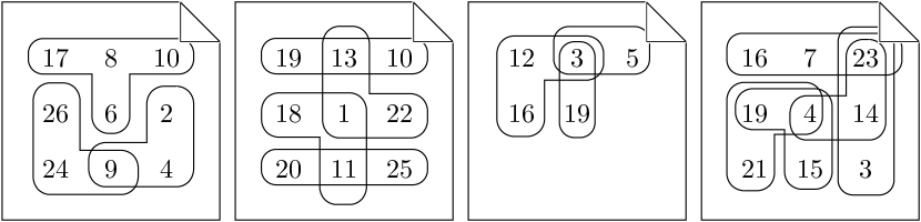
Figure 1: Application of Pagination to the visualization of the cliques of a given graph. The cliques are split over a small number of pages (here, 4) with a given capacity (here, at most 9 vertices). To allow each clique to be entirely contained in a single page, some vertices may be repeated on different pages (here, 19 on 3 pages, and 3, 4, 10, 16 on 2 pages). The individual page layouts are not relevant.

For instance, the members of a social network may interest us only to the extent that they are part of one or several friendship circles. Such groups of mutual friends are nothing more than the so-called cliques of a graph (Fig. 1, upper), but the cliques are notoriously difficult to extract visually. Visualizing them as separated sets of vertices is more effective, although quite redundant. A better compromise between compacity and clarity is attained by paginating these sets as in Fig. 1 (lower part). Note that, although no group is scattered across several pages, finding all the friends of a given person may require the consultation of several pages.

1.2 Definition and complexity

Our problem is not just about visualization. It extends to any need of segmentation of partially redundant data (see Section 1.3.1 for an application to virtual machine colocation). Let us define it in the most general way:

Definition 1.

Pagination can be expressed as the following decision problem:

• Input: a finite collection $\mathcal{T}$ of nonempty finite sets (the tiles) of symbols, an integer $C>0$ (the capacity) and an integer $n>0$ (the number of pages).

• Question: does there exist an $n$-way partition (or pagination) $\mathcal{P}$ of $\mathcal{T}$ such that, for any tile set (or page) $p$ of $\mathcal{P}$, $|\cup_{t\in p}t|\leq C$?

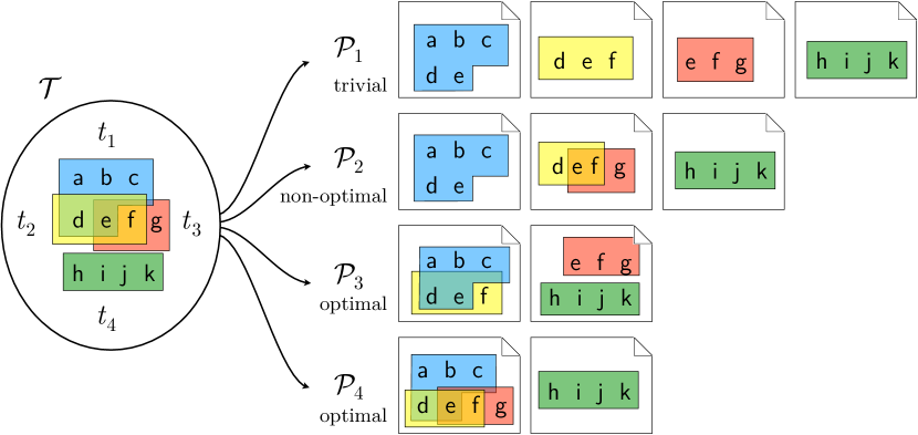
Figure 2: For the tiles $\mathcal{T}=\{\hbox{\pagecolor{tileColor}\color[rgb]{1,1,1}{\text{\sf{abcde}}}}\,\allowbreak\hbox{\pagecolor{tileColor}\color[rgb]{1,1,1}{\text{\sf{def}}}}\,\allowbreak\hbox{\pagecolor{tileColor}\color[rgb]{1,1,1}{\text{\sf{efg}}}}\,\allowbreak\hbox{\pagecolor{tileColor}\color[rgb]{1,1,1}{\text{\sf{hijk}}}}\}$ and a capacity $C=7$, $\mathcal{P}_{3}=(\{\hbox{\pagecolor{tileColor}\color[rgb]{1,1,1}{\text{\sf{abcde}}}}\,\allowbreak\hbox{\pagecolor{tileColor}\color[rgb]{1,1,1}{\text{\sf{def}}}}\},\allowbreak\{\hbox{\pagecolor{tileColor}\color[rgb]{1,1,1}{\text{\sf{efg}}}}\,\allowbreak\hbox{\pagecolor{tileColor}\color[rgb]{1,1,1}{\text{\sf{hijk}}}}\})$ is a possible optimal pagination in $n=2$ pages.

Example 1.

On the left of Fig. 2, $\mathcal{T}=\{\{\textsf{a},\textsf{b},\textsf{c},\textsf{d},\textsf{e}\}$, $\{\textsf{d},\textsf{e},\textsf{f}\}$, $\{\textsf{e},\textsf{f},\textsf{g}\}$, $\{\textsf{h},\textsf{i},\textsf{j},\textsf{k}\}\}$ denotes the tiles to be distributed on pages (with respect to a given capacity of 7). On the right, we present 4 possible such paginations of this set. For easier reading, in the remainder of this paper, any set of symbols (especially, a tile) defined by extension (for instance, $\{\textsf{w},\textsf{o},\textsf{r},\textsf{d}\}$) will be represented as a gray block: word. Moreover, in any collection of symbol sets (especially $\mathcal{T}$, or a page), the separating commas will be omitted: $\{\hbox{\pagecolor{tileColor}\color[rgb]{1,1,1}{\text{\sf{May}}}}$ June $\hbox{\pagecolor{tileColor}\color[rgb]{1,1,1}{\text{\sf{July}}}}\}$.

Proposition 1.

Pagination is NP-complete in the strong sense.

Proof.

Any given pagination $\mathcal{P}$ can be verified in polynomial time. Furthermore, Bin Packing is a special case of Pagination with no shared symbol. Hence, the latter is at least as difficult as the former, which is strongly NP-complete. ∎

In the rest of this paper, we focus on the associated NP-hard optimization problem (i.e., where the aim is to minimize the number of pages).

1.3 Related works

Bin Packing and its numerous variants are among the most studied optimization problems, and, as such, regularly subjected to comprehensive surveys [2, 3, 11, 15]. The purpose of the present section is far more limited: to extract from this vast literature the few problems which exhibit the distinguishing feature of Pagination, i.e., which deal with objects able to overlap in a non-additive fashion. For instance, despite its similar name, we will not discuss Newspaper Pagination, a Bin Packing variant studied in [14] for the placement of (obviously non overlapping) blocks of text on the columns of a generalized newspaper.

1.3.1 Virtual machine allocation

Pagination was first introduced in 2011 by Sindelar et al. [19] in the context of virtual machine (VM) colocation. A VM can be seen as a set of memory pages: although most of them belong exclusively to one machine, some pages are identical across several machines. This happens more often as the configurations are close in terms of platform, system version, software libraries, or installed applications. If these VM run on the same physical server, their common memory pages can actually be pooled in order to spare resources.

The authors study two related problems. The first one, VM Maximization, is defined as follows: being given a collection of VM (our tiles), each consisting in a set of memory pages (our symbols), determine the most profitable subset of VM that can be packed into a given set of servers (our pages) having a capacity of $k$ memory pages (of $C$ symbols). Note that, with one server, this problem can be seen equivalently as Knapsack with Overlapping Items [8], or Densest k-subhypergraph. Hajiaghayi et al. [10] have proven the latter to be hard to approximate within a factor of $2^{(\log n)^{\delta}}$ for some $\delta>0$, and Rampersaud and Grosu [17] approximated it by a greedy heuristic with an approximation ratio equal to the number of VM. Furthermore, when the sharing among VM occurs in certain hierarchical fashions, Sindelar et al. have used a left-right dynamic programming method to devise a fully-polynomial time approximation scheme (FPTAS) [19].

The second problem, VM Packing, is nothing else than Pagination: it demands to allocate the VM to a minimal number of servers. Sindelar et al. have shown that repeating their dynamic programming algorithm solves it within a $O(\log n)$ factor in a clustered version of the hierarchical model; and that a greedy algorithm achieves a factor of $3$ when each cluster is a singleton.

Although these hierarchical restrictions lead to provably-good approximations algorithms, they say nothing about the general model, which the authors left open [19]. Thereafter, efforts have mainly focused on models and methods designed specifically for the purposes of solving real-world VM allocation problems (e.g., [18] with multiple resource requirements in an online setting, or [22] for approaches based on genetic algorithms): as far as we know, the general case has been left unexplored. In the interest of differentiating it from these VM-oriented models, we take the liberty to replace the terms of VM packing, memory pages, VM and servers, by the application-agnostic terms of Pagination, symbols, tiles and pages (respectively).

1.3.2 Hypergraph partitioning

Let us recall that a hypergraph $G=(V,E)$ is defined by a set of vertices $V$ and a set of hyperedges $E$, where each element of $E$ is a subset of $V$ [1]. Bearing this in mind, it is easy to see the left-hand part of Fig. 2 as a subset-based drawing [13] of a hypergraph mapping the instance, namely with $V=\mathcal{A}$ (the set of vertices is the set of symbols) and $E=\mathcal{T}$ ((the set of hyperedges is the set of tiles). Since Pagination is a partitioning problem, it is natural to ask whether we could take advantage of the extensive literature on Hypergraph Partitioning. In [12] for instance, the latter problem is defined as “partitioning the vertices of a hypergraph into $k$ roughly equal parts, such that a certain objective function defined over the hyperedges is optimized”. Although our capacity constraint on the symbols is reminiscent of this “roughly equal” number of vertices, the main purpose of Pagination is to partition the tiles (i.e., the hyperedges), and certainly not the symbols (i.e., the vertices).

So, what happens if we try to exchange the roles of the tiles and the symbols? This gives the following alternative hypergraph representation of the instances of Pagination: $V=\mathcal{T}$ (the vertices are the tiles) and $E=\mathcal{A}$ (the hyperedges are the symbols). To be more specific, a symbol shared by several tiles connects them as a hyperedge, while a proper symbol (i.e., a symbol belonging to one tile only) connects this tile to itself as a hyperloop. Now, paginating $G$ indeed amounts to partitioning the vertices, but in the meantime two issues have arisen. First, we do not care if each part contains roughly the same number of tiles: we want instead that the number of involved hyperedges is at most equal to $C$. Second, we have to express our objective function (minimizing the number of pages) on the hyperedges (the symbols). To cite [12] again: “a commonly used objective function is to minimize the number of hyperedges that span different partitions”. At first sight, it would indeed seem reasonable to minimize the number of replications of a given symbol across the pages. However, this leads to another impasse:

Proposition 2.

Minimizing the number of pages and minimizing the number of symbol replications are not equivalent.

counterexample.

For $C=5$, let $\mathcal{T}=\{\hbox{\pagecolor{tileColor}\color[rgb]{1,1,1}{\text{\sf{a1}}}}\,\allowbreak\hbox{\pagecolor{tileColor}\color[rgb]{1,1,1}{\text{\sf{357}}}}\,\allowbreak\hbox{\pagecolor{tileColor}\color[rgb]{1,1,1}{\text{\sf{a2}}}}\,\allowbreak\hbox{\pagecolor{tileColor}\color[rgb]{1,1,1}{\text{\sf{468}}}}\}$. The optimal pagination $\{\{\hbox{\pagecolor{tileColor}\color[rgb]{1,1,1}{\text{\sf{a1}}}}\,\allowbreak\hbox{\pagecolor{tileColor}\color[rgb]{1,1,1}{\text{\sf{357}}}}\},\allowbreak\{\hbox{\pagecolor{tileColor}\color[rgb]{1,1,1}{\text{\sf{a2}}}}\,\allowbreak\hbox{\pagecolor{tileColor}\color[rgb]{1,1,1}{\text{\sf{468}}}}\}\}$ minimizes the number of pages (2), but not the number of replicas (symbol a is replicated once). Conversely, the non-optimal pagination $\{\{\hbox{\pagecolor{tileColor}\color[rgb]{1,1,1}{\text{\sf{a1}}}}\,\allowbreak\hbox{\pagecolor{tileColor}\color[rgb]{1,1,1}{\text{\sf{a2}}}}\},\{\hbox{\pagecolor{tileColor}\color[rgb]{1,1,1}{\text{\sf{357}}}}\},\allowbreak\{\hbox{\pagecolor{tileColor}\color[rgb]{1,1,1}{\text{\sf{468}}}}\}\}$ minimizes the number of symbol replications (0), but not the number of pages (3). ∎

Therefore, contrary to appearances, Pagination has very little in common with Hypergraph Partitioning.

The rest of this paper is organized as follows. In Section 2, we formulate Pagination as an integer linear program (ILP), and introduce the various metrics and rules used by our algorithms. Then, in Section 3, we describe several heuristics and meta-heuristics for the problem. Finally, we compare the results produced by all the algorithms (exact or not) in Section 4, and conclude in Section 5.

2 Theoretical tools

To look on our problem from another perspective, let us formulate it as an ILP problem. In addition, we will be able to solve some (admittedly simple) instances with a generic optimization software. Thereafter, the introduction of several supplementary concepts will permit us to actually generate the instances, and to describe our own algorithms for tackling the largest ones.

2.1 Integer linear programming model

Numberings

We use the following sets of indexes:

• $A=\{i:i=1,\dots,|\mathcal{A}|\}$ for the symbols;

• $T=\{j:j=1,\dots,|\mathcal{T}|\}$ for the tiles;

• $P=\{k:k\in\mathbb{N}\}$ for the pages.

Inputs

• $C$ is a strictly positive integer capacity;

• $a^{i}_{j}$ is an assignment of symbols to tiles: $\forall i\in A,\forall j\in T,a^{i}_{j}=1$ if $i\in t_{j}$, and 0 otherwise.

Decision variables

For any $i\in A$, $j\in T$ and $k\in P$, we define:

• $x^{i}_{k}$ as equal to 1 if symbol $i$ is present on page $k$, and 0 otherwise (pagination of the symbols);

• $y^{j}_{k}$ as equal to 1 if tile $j$ is present on page $k$, and 0 otherwise (pagination of the tiles);

• $z_{k}$ as equal to 1 if page $k$ is used, and 0 otherwise (unitary usage of the pages).

It is worth noting that $x^{i}_{k}=\max_{j\in T}(a^{i}_{j}y^{j}_{k})$ and $z_{k}=\max_{j\in T}(y^{j}_{k})$. The mathematical model of Pagination is thus entirely specified with $y^{j}_{k}$: the introduction of these auxiliary variables is only used to achieve the linearity of its formulation.

Integer linear program

A possible ILP formulation of Pagination is:

min. $$\sum_{k\in P}z_{k}$$

s. t. $$\sum_{k\in P}y^{j}_{k}=1, \forall j\in T$$ (1)

$$z_{k}\geq x^{i}_{k}, \forall i\in A,\forall k\in P$$ (2)

$$\sum_{i\in A}x^{i}_{k}\leq z_{k}C, \forall k\in P$$ (3)

$$x^{i}_{k}\geq a^{i}_{j}y^{j}_{k}, \forall i\in A,\forall j\in T,\forall k\in P$$ (4)

$$x^{i}_{k},\;y^{j}_{k},z_{k}\;\text{all binary,} \forall i\in A,\forall j\in T,\forall k\in P$$ (5)

Eq. 1 assigns each tile to exactly one page. Eq. 2 ensures that a page is used as soon as it contains one symbol. Conversely, thanks to the objective function, every used page contains at least one symbol. From Eq. 3, a page cannot contain more than $C$ symbols. Eq. 4 guarantees that, when a tile belongs to a page, this page includes all its symbols. The integrality constraints of the auxiliary variables of Eq. 5 could be relaxed.

2.2 Counting of the symbols

Definition 2 (metrics).

Let $\alpha$ be a symbol, $t$ a tile and $p$ a set of tiles (most often, a page). Then:

1. the size $|t|$ of $t$ is its number of symbols;

2. the volume $\mathcal{V}(p)$ of $p$ is its number of distinct symbols: $\mathcal{V}(p)=|\cup_{t\in p}t|$; and its complement $C-\mathcal{V}(p)$, the loss on $p$;

3. by contrast, the cardinality $\mathrm{Card}(p)$ is the total number of symbols (distinct or not) in $p$: $\mathrm{Card}(p)=\sum_{t\in p}|t|$.

4. the multiplicity $\mu_{p}(\alpha)$ counts the occurrences of $\alpha$ in the tiles of $p$: $\mu_{p}(\alpha)=|\{t\in p:\alpha\in t\}|$;

5. the relative size of $t$ on $p$ is the sum of the reciprocals of the multiplicities of the symbols of $t$ in $p$: $|t|_{p}=\sum_{\alpha\in t}\frac{1}{\mu_{p}(\alpha)}$.

In recognition of the fact that a given symbol may occur several times on the same page, the terms cardinality and multiplicity are borrowed from the multiset theory [21].

Example 2.

In pagination $\mathcal{P}_{3}$ of Fig. 2: size $|t_{1}|=5$, volume $\mathcal{V}(p_{1})=6$ (loss: $7-6$), cardinality $\mathrm{Card}(p_{1})=5+3$, multiplicity $\mu_{p_{1}}(\textsf{e})=2$, relative size $|t_{2}|_{p_{1}}=1/2+1/2+1$.

These definitions are extended to several pages (i.e., sets of sets of tiles) by summing the involved values:

Example 3.

In the same figure, volume $\mathcal{V}(\mathcal{P}_{3})=6+7$ (loss: $7-1+7-7$), cardinality $\mathrm{Card}(\mathcal{P}_{3})=\mathrm{Card}(\mathcal{T})=5+3+3+4$, multiplicity $\mu_{\mathcal{P}_{3}}(\textsf{e})=\mu_{\mathcal{T}}(\textsf{e})=2+1$, relative size $|t_{2}|_{\mathcal{P}_{3}}=|t_{2}|_{\mathcal{T}}=1/2+1/3+1/2$.

We are now able to express a first interesting difference with Bin Packing:

Proposition 3.

A pagination whose loss is minimal is not necessarily optimal.

counterexample.

For $C=4$, the tile set $\mathcal{T}=\{\hbox{\pagecolor{tileColor}\color[rgb]{1,1,1}{\text{\sf{12}}}}\,\allowbreak\hbox{\pagecolor{tileColor}\color[rgb]{1,1,1}{\text{\sf{13}}}}\,\allowbreak\hbox{\pagecolor{tileColor}\color[rgb]{1,1,1}{\text{\sf{23}}}}\,\allowbreak\hbox{\pagecolor{tileColor}\color[rgb]{1,1,1}{\text{\sf{ab}}}}\,\allowbreak\hbox{\pagecolor{tileColor}\color[rgb]{1,1,1}{\text{\sf{ac}}}}\,\allowbreak\hbox{\pagecolor{tileColor}\color[rgb]{1,1,1}{\text{\sf{bc}}}}\}$ has a loss of $1+1$ on the optimal pagination $(\{\hbox{\pagecolor{tileColor}\color[rgb]{1,1,1}{\text{\sf{12}}}}\,\allowbreak\hbox{\pagecolor{tileColor}\color[rgb]{1,1,1}{\text{\sf{13}}}}\,\allowbreak\hbox{\pagecolor{tileColor}\color[rgb]{1,1,1}{\text{\sf{23}}}}\},\allowbreak\{\hbox{\pagecolor{tileColor}\color[rgb]{1,1,1}{\text{\sf{ab}}}}\,\allowbreak\hbox{\pagecolor{tileColor}\color[rgb]{1,1,1}{\text{\sf{ac}}}}\,\allowbreak\hbox{\pagecolor{tileColor}\color[rgb]{1,1,1}{\text{\sf{bc}}}}\})$; but a loss of $0+0+0$ on the non-optimal pagination $(\{\hbox{\pagecolor{tileColor}\color[rgb]{1,1,1}{\text{\sf{12}}}}\,\allowbreak\hbox{\pagecolor{tileColor}\color[rgb]{1,1,1}{\text{\sf{ab}}}}\},\allowbreak\{\hbox{\pagecolor{tileColor}\color[rgb]{1,1,1}{\text{\sf{13}}}}\,\allowbreak\hbox{\pagecolor{tileColor}\color[rgb]{1,1,1}{\text{\sf{ac}}}}\},\allowbreak\{\hbox{\pagecolor{tileColor}\color[rgb]{1,1,1}{\text{\sf{23}}}}\,\allowbreak\hbox{\pagecolor{tileColor}\color[rgb]{1,1,1}{\text{\sf{bc}}}}\})$. ∎

As seen in this counterexample, for the complete page set, multiplicity, cardinality and relative size do not depend on the pagination. Then:

Proposition 4.

A pagination is optimal if and only if the average cardinality of its pages is maximal.

Proof.

Since the sum of the page cardinalities is always equal to $\sum_{t\in\mathcal{T}}|t|$, its average depends only of the size $n$ of the pagination. Hence, minimizing this size or that average is equivalent. ∎

2.3 Simplifying assumptions

Definition 1 encompasses many instances whose pagination is either infeasible (e.g., one tile exceeds the capacity), trivial (e.g., all tiles can fit in one page) or reducible (e.g., one tile is a subset of another one). The purpose of this subsection is to bring us closer to the core of the problem, by ruling out as many such degenerated cases as possible. For each one, we prove that there is nothing lost for an offline algorithm to ignore the corresponding instances.

Rule 1.

No tile is included in another one: $\forall(t,t^{\prime})\in\mathcal{T}^{2}:t\neq t^{\prime},t\not\subseteq t^{\prime}$.

Proof.

If $t\subseteq t^{\prime}$, then $t$ and $t^{\prime}$ can be put together on the same page of the optimal solution. ∎

Remark 1.

This does not hold for an online algorithm. Take for instance $\mathcal{T}=\{\hbox{\pagecolor{tileColor}\color[rgb]{1,1,1}{\text{\sf{12}}}}\,\allowbreak\hbox{\pagecolor{tileColor}\color[rgb]{1,1,1}{\text{\sf{345}}}}\,\allowbreak\hbox{\pagecolor{tileColor}\color[rgb]{1,1,1}{\text{\sf{126}}}}\,\allowbreak\hbox{\pagecolor{tileColor}\color[rgb]{1,1,1}{\text{\sf{378}}}}\}$ and $C=5$. If the tiles are presented in this order, the first two may be placed on the first page, making necessary to create a new page for each remaining tile: $\{\{\hbox{\pagecolor{tileColor}\color[rgb]{1,1,1}{\text{\sf{12}}}}\,\allowbreak\hbox{\pagecolor{tileColor}\color[rgb]{1,1,1}{\text{\sf{345}}}}\},\{\hbox{\pagecolor{tileColor}\color[rgb]{1,1,1}{\text{\sf{126}}}}\},\{\hbox{\pagecolor{tileColor}\color[rgb]{1,1,1}{\text{\sf{378}}}}\}\}$. An optimal pagination would require two pages only: $\{\{\hbox{\pagecolor{tileColor}\color[rgb]{1,1,1}{\text{\sf{12}}}}\,\allowbreak\hbox{\pagecolor{tileColor}\color[rgb]{1,1,1}{\text{\sf{126}}}}\},\{\hbox{\pagecolor{tileColor}\color[rgb]{1,1,1}{\text{\sf{346}}}}\,\allowbreak\hbox{\pagecolor{tileColor}\color[rgb]{1,1,1}{\text{\sf{378}}}}\}\}$.

In other words, the tile sets we deal with are Sperner families [20]. It follows that:

Corollary 1 (Sperner’s Theorem).

A page of capacity $C$ contains at most $\binom{C}{\lfloor C/2\rfloor}$ tiles.

Rule 2.

No tile contains all the symbols: $\nexists t\in\mathcal{T}:t=\mathcal{A}$.

Proof.

Direct consequence of Rule 1. ∎

Rule 3.

Each tile has less than $C$ symbols: $\forall t\in\mathcal{T},|t|<C$.

Proof.

Let $t$ be an arbitrary tile. If $|t|>C$, the problem has no solution. If $|t|=C$, then no other tile $t^{\prime}$ could appear on the same page as $t$ without violating Rule 1. Let $\mathcal{P}^{\prime}$ be an optimal pagination of the reduced instance $\mathcal{T}\setminus\{t\}$. Then $\mathcal{P}=\mathcal{P}^{\prime}\cup\{\{t\}\}$ is an optimal pagination of $\mathcal{T}$. ∎

Rule 4.

No symbol is shared by all tiles: $\nexists\alpha\in\mathcal{A}:\forall t\in\mathcal{T},\alpha\in t$.

Proof.

Otherwise, let $\mathcal{P}^{\prime}$ be an optimal pagination, for a capacity of $C-1$, of the reduced instance $\mathcal{T}^{\prime}=\{t\setminus\alpha:t\in\mathcal{T}\text{~{}and~{}}t\neq\{\alpha\}\}$. Then adding $\alpha$ to each page of $\mathcal{P}^{\prime}$ gives an optimal pagination $\mathcal{P}$ of $\mathcal{T}$ for capacity $C$. Should a tile $\{\alpha\}$ exist in $\mathcal{T}$, it can be put back at no cost on any page of $\mathcal{P}$. ∎

In other words, $\mathcal{T}$ has not the Helly property [5]. Contrast this with VM Packing [19], where the mere existence of root symbols violates this rule.

Rule 5.

Each symbol belongs to at least one tile: $\forall\alpha\in\mathcal{A},\exists t\in\mathcal{T}:\alpha\in t$.

Proof.

By Definition 1 of an instance. ∎

Rule 6.

Each tile is compatible with at least another one: $\forall t\in\mathcal{T},\exists t^{\prime}\in\mathcal{T}\setminus\{t\}:|t\cup t^{\prime}|\leq C$.

Proof.

If there exists a tile $t$ not compatible with any other, any solution should devote a complete page to $t$. The conclusion of the proof of Rule 3 still applies here. ∎

Rule 7.

$C>2$.

Proof.

Since all tiles contain at least one symbol, Rule 3 implies $C\geq 2$. Assume that $C=2$, i.e., all tiles consist in one single symbol. Hence, $\{\{t_{1},t_{2}\},\{t_{3},t_{4}\},...\}$ is an optimal pagination of $\mathcal{T}$ in $\lceil{\frac{|\mathcal{T}|}{2}\rceil}$ pages. ∎

Rule 8.

$C<|\mathcal{A}|$.

Proof.

Otherwise, all tiles could fit in one page. ∎

To sum up, an optimal solution of an instance violating Rules 1, 3 (with $|t|=C$), 4, 5 or 6, could be deduced from an optimal solution of this instance deprived of the offending tiles or symbols; an instance violating Rule 3 (with $|t|>C$) would be infeasible; an instance violating Rules 2, 7 or 8 would be trivial. All these rules can be tested in polynomial time, and are actually required by our instance generator (Section 4.1).

3 Heuristics

In this section, we investigate four families of heuristics for Pagination, from the simplest to the most sophisticated one. The first family consists of direct adaptations of the well-studied Bin Packing’s greedy Any Fit algorithms; we show that, in Pagination, their approximation factor cannot be bounded. The second family is similar, but relies on the overlapping property specific to our problem; a general instance is devised, which shows that the approximation factor of their offline version is at least 3. With the third algorithm, we leave the realm of greedy decisions for a slightly more complex, but hopefully more efficient strategy, based upon a reentering queue. Finally, we present two genetic algorithms and discuss which encoding and cost function are better suitable to Pagination. All of this is carried out from a theoretical perspective, the next section being devoted to the presentation of our benchmarks.

3.1 Greedy heuristics inspired from Bin Packing

3.1.1 Definitions

The question naturally arises of how the Bin Packing classical approximation algorithms [2] behave in the more general case of Pagination. Let us enumerate a few of them with our terminology:

• Next Fit simply stores each new tile in the last created page or, should it exceed the capacity, in a newly created page.

• First Fit rescans sequentially the pages already created, and puts the new tile in the first page where it fits.

• Best Fit always chooses the fullest page, i.e., the page with maximal volume. Such a criterion needs to be clarified in our generalization of Bin Packing: fullest before or after having put the new tile? This alternative should give rise to two variants.

• Worst Fit, contrary to Best Fit, favors the less full page.

• Almost Worst Fit is a variant of Worst Fit opting for the second less full page.

These algorithms are known under the collective name of Any Fit (AF). In their offline version, pre-sorting the items by size has a positive impact on their packing; but for Pagination, such a sorting criterion would obviously be defective: due to possible merges, a large tile often occupies less volume than a small one.

3.1.2 A general unfavorable case

Regardless of its scheduling (online or offline), no AF algorithm has performance guarantee on the following extensible Pagination instance.

Let $C$ be an even capacity ($C=4$ on Fig. 3). Let $\mathcal{A}_{\alpha}=\{\alpha_{1},...,\alpha_{C}\}$ and $\mathcal{A}_{\beta}=\{\beta_{1},...,\beta_{C}\}$ be two sets of distinct symbols such that $\mathcal{A}$ is the disjoint union of $\mathcal{A}_{\alpha}$ and $\mathcal{A}_{\beta}$. Let $\mathcal{T}_{\alpha}=\binom{\mathcal{A}_{\alpha}}{C/2}$ and $\mathcal{T}_{\beta}=\binom{\mathcal{A}_{\beta}}{C/2}$ be the set of the $\frac{C}{2}$-combinations of $\mathcal{A}_{\alpha}$ and $\mathcal{A}_{\beta}$ (respectively). Then $\mathcal{P}_{\textrm{opt}}=\{\mathcal{T}_{\alpha},\mathcal{T}_{\beta}\}$ is an optimal pagination of $\mathcal{T}=\mathcal{T}_{\alpha}\cup\mathcal{T}_{\beta}$ in $2$ pages.

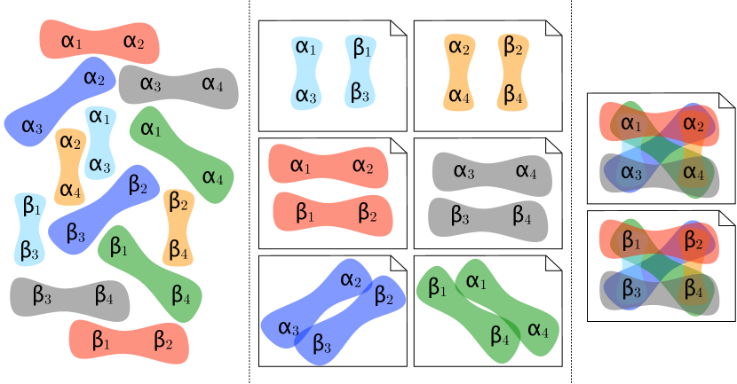
Figure 3: To the left, a set $\mathcal{T}=\mathcal{T}_{\alpha}\cup\mathcal{T}_{\beta}$ of $2\binom{4}{2}=12$ tiles; at the center, a pagination of capacity $4$ calculated by the Any Fit algorithms when the tiles of $\mathcal{T}_{\alpha}$ and $\mathcal{T}_{\beta}$ are fed alternatively; to the right, an optimal pagination.

Now, let us feed these tiles to any of our AF algorithms, but only after having sorted them in the worst order: since all of our tiles have the same size $C/2$, we are indeed free to organize them the way we want. The most unfavorable schedule simply involves alternating the tiles of $\mathcal{T}_{\alpha}$ and $\mathcal{T}_{\beta}$. In this way, regardless of the selected AF algorithm, the first two tiles would saturate the first page, the next two, the second page, and so on. In total, an AF algorithm would then create $n=|\mathcal{T}_{\alpha}|=|\mathcal{T}_{\beta}|=\binom{C}{C/2}=\frac{C!}{(C/2)!^{2}}$ pages instead of 2. In this family, the approximation factor is thus unbounded. This stands in stark contrast to the efficiency of the AF algorithms on Bin Packing—where, for instance, First Fit was recently shown [4] to achieve an absolute factor of exactly 1.7.

3.1.3 Study case: First Fit algorithm

For our tests, we have chosen to focus on First Fit (in its online version). The worst case complexity can be analyzed as follows. There are $|\mathcal{T}|$ tiles to paginate. At worst, according to Rule 6, there exists only one tile compatible with any other, resulting in $|\mathcal{T}|-1$ pages. Lastly, each set intersection costs a linear time in the size of the candidate tile. Hence, the overall complexity is $\mathcal{O}(|\mathcal{T}|^{2}\mathrm{Card}(\mathcal{T}))$.

Note that in Bin Packing, for $n$ items, an appropriate data structure can reduce the straightforward quadratic complexity to $\mathcal{O}(n\log(n))$ [11]. This optimization is not applicable here, where the current volume of a given page says little about its ability to accommodate a given tile.

3.2 Specialized greedy heuristics

3.2.1 Definition

We can easily improve on the Bin Packing heuristics by taking into account the merging property of Pagination items.

The corresponding offline greedy algorithms always select, among the remaining tiles, the one which minimizes or maximizes a certain combination of the metrics introduced in Definition 2 (e.g., volume, multiplicity, relative size, etc.). In their online version, since the new tile is given, this optimization relies only on the past assignments.

3.2.2 A general unfavorable case

Before introducing the particular heuristic we have the most thoroughly tested, Best Fusion, let us mark out the limitations of the algorithms of this family. We will design an extensible instance whose all tiles are equivalent with respect to these metrics. As such, they may be taken in any order, including the worst, which ensures that the reasoning is valid for both online and offline scheduling.

Take an even capacity $C$, and $\mathcal{A}_{0}=\{\alpha_{1},...,\alpha_{C}\}$ a first subset of $\mathcal{A}$. Let $\mathcal{T}_{0}=\binom{\mathcal{A}_{0}}{C-1}$ the $(C-1)$-combinations of $\mathcal{A}_{0}$, which amount to $C$ tiles of size $C-1$. From now on, to better understand the general construction, we will illustrate each step on an example with $C=4$:

$$\mathcal{A}_{0}=\hbox{\pagecolor{tileColor}\color[rgb]{1,1,1}{\text{\sf{1234}}}},\qquad\mathcal{T}_{0}=\{\hbox{\pagecolor{tileColor}\color[rgb]{1,1,1}{\text{\sf{123}}}}\,\hbox{\pagecolor{tileColor}\color[rgb]{1,1,1}{\text{\sf{124}}}}\,\hbox{\pagecolor{tileColor}\color[rgb]{1,1,1}{\text{\sf{134}}}}\,\hbox{\pagecolor{tileColor}\color[rgb]{1,1,1}{\text{\sf{234}}}}\}$$

Introduce two more symbols, namely a and b, which will be used to lock the pages. Partition $\mathcal{T}$ into $\frac{C}{2}$ couples of tiles: ${(t_{1},t_{2}),(t_{3},t_{4}),...,(t_{C-1},t_{C})}$. From each such couple, form $\mathcal{A}_{i}=(t_{2i-1}\cap t_{2i})\cup\{\textsf{a},\textsf{b}\}$ with $1\leq i\leq\frac{C}{2}$, a subset of $\mathcal{A}$. In the same way as on $\mathcal{A}_{0}$, define $\mathcal{T}_{i}=\binom{\mathcal{A}_{i}}{C-1}$ on each $\mathcal{A}_{i}$:

$$\mathcal{A}_{1} =\hbox{\pagecolor{tileColor}\color[rgb]{1,1,1}{\text{\sf{12ab}}}},\qquad\mathcal{T}_{1}=\{\hbox{\pagecolor{tileColor}\color[rgb]{1,1,1}{\text{\sf{12a}}}}\,\hbox{\pagecolor{tileColor}\color[rgb]{1,1,1}{\text{\sf{12b}}}}\,\hbox{\pagecolor{tileColor}\color[rgb]{1,1,1}{\text{\sf{1ab}}}}\,\hbox{\pagecolor{tileColor}\color[rgb]{1,1,1}{\text{\sf{2ab}}}}\}$$

$$\mathcal{A}_{2} =\hbox{\pagecolor{tileColor}\color[rgb]{1,1,1}{\text{\sf{34ab}}}},\qquad\mathcal{T}_{2}=\{\hbox{\pagecolor{tileColor}\color[rgb]{1,1,1}{\text{\sf{34a}}}}\,\hbox{\pagecolor{tileColor}\color[rgb]{1,1,1}{\text{\sf{34b}}}}\,\hbox{\pagecolor{tileColor}\color[rgb]{1,1,1}{\text{\sf{3ab}}}}\,\hbox{\pagecolor{tileColor}\color[rgb]{1,1,1}{\text{\sf{4ab}}}}\}$$

Constructing this instance is actually constructing an optimal solution to it. Indeed, for the whole tile set, $|\mathcal{P}_{\textrm{opt}}|=\frac{C}{2}+1$:

$$p_{1} =\{\hbox{\pagecolor{tileColor}\color[rgb]{1,1,1}{\text{\sf{123}}}}\,\hbox{\pagecolor{tileColor}\color[rgb]{1,1,1}{\text{\sf{124}}}}\,\hbox{\pagecolor{tileColor}\color[rgb]{1,1,1}{\text{\sf{134}}}}\,\hbox{\pagecolor{tileColor}\color[rgb]{1,1,1}{\text{\sf{234}}}}\}\rightarrow\hbox{\pagecolor{tileColor}\color[rgb]{1,1,1}{\text{\sf{1234}}}}$$

$$p_{2} =\{\hbox{\pagecolor{tileColor}\color[rgb]{1,1,1}{\text{\sf{12a}}}}\,\hbox{\pagecolor{tileColor}\color[rgb]{1,1,1}{\text{\sf{12b}}}}\,\hbox{\pagecolor{tileColor}\color[rgb]{1,1,1}{\text{\sf{1ab}}}}\,\hbox{\pagecolor{tileColor}\color[rgb]{1,1,1}{\text{\sf{2ab}}}}\}\rightarrow\hbox{\pagecolor{tileColor}\color[rgb]{1,1,1}{\text{\sf{12ab}}}}$$

$$p_{3} =\{\hbox{\pagecolor{tileColor}\color[rgb]{1,1,1}{\text{\sf{34a}}}}\,\hbox{\pagecolor{tileColor}\color[rgb]{1,1,1}{\text{\sf{34b}}}}\,\hbox{\pagecolor{tileColor}\color[rgb]{1,1,1}{\text{\sf{3ab}}}}\,\hbox{\pagecolor{tileColor}\color[rgb]{1,1,1}{\text{\sf{4ab}}}}\}\rightarrow\hbox{\pagecolor{tileColor}\color[rgb]{1,1,1}{\text{\sf{34ab}}}}$$

Now, let us construct a non-optimal pagination. This is done by pairing each tile of $\mathcal{T}_{0}$ with a tile including a “locking” symbol. Specifically, on pages $2i-1$ and $2i$, put respectively $t_{2i-1}$ and $t_{2i}$, and lock these pages with tiles $(t_{2i-1}\cap t_{2i})\cup\{\textsf{a}\}$ and $(t_{2i-1}\cap t_{2i})\cup\{\textsf{b}\}$ (respectively) from $\mathcal{T}_{i}$. This process creates $C$ locked pages:

$$p^{\prime}_{1} =\{\hbox{\pagecolor{tileColor}\color[rgb]{1,1,1}{\text{\sf{123}}}}\,\hbox{\pagecolor{tileColor}\color[rgb]{1,1,1}{\text{\sf{12a}}}}\}\rightarrow\hbox{\pagecolor{tileColor}\color[rgb]{1,1,1}{\text{\sf{123a}}}}$$

$$p^{\prime}_{2} =\{\hbox{\pagecolor{tileColor}\color[rgb]{1,1,1}{\text{\sf{124}}}}\,\hbox{\pagecolor{tileColor}\color[rgb]{1,1,1}{\text{\sf{12b}}}}\}\rightarrow\hbox{\pagecolor{tileColor}\color[rgb]{1,1,1}{\text{\sf{124b}}}}$$

$$p^{\prime}_{3} =\{\hbox{\pagecolor{tileColor}\color[rgb]{1,1,1}{\text{\sf{134}}}}\,\hbox{\pagecolor{tileColor}\color[rgb]{1,1,1}{\text{\sf{34a}}}}\}\rightarrow\hbox{\pagecolor{tileColor}\color[rgb]{1,1,1}{\text{\sf{134a}}}}$$

$$p^{\prime}_{4} =\{\hbox{\pagecolor{tileColor}\color[rgb]{1,1,1}{\text{\sf{234}}}}\,\hbox{\pagecolor{tileColor}\color[rgb]{1,1,1}{\text{\sf{34b}}}}\}\rightarrow\hbox{\pagecolor{tileColor}\color[rgb]{1,1,1}{\text{\sf{234b}}}}$$

But what enables us to construct such inefficient two-tile pages? All tiles having the same size, it is clear that the first one can be chosen arbitrarily. Now, let $t^{\prime}$ be an eligible second tile, and $p^{\prime}$ the resulting page. Then, all $t^{\prime}$ are equivalent under our various metrics: same size $|t^{\prime}|=C-1$, same volume $\mathcal{V}(p^{\prime})=C$, same cardinality $\mathrm{Card}(p^{\prime})=2(C-1)$, same relative size $|t^{\prime}|_{p^{\prime}}=\frac{C-2}{2}+1=\frac{C}{2}$. So, nothing prevents our greedy algorithms to systematically select the worst candidate.

If $C>2$, the $C-2$ tiles including both a and b still remain in every tile set (but $\mathcal{T}_{0}$). For each one, gather its tiles on a new page:

$$p^{\prime}_{5} =\{\hbox{\pagecolor{tileColor}\color[rgb]{1,1,1}{\text{\sf{1ab}}}}\,\hbox{\pagecolor{tileColor}\color[rgb]{1,1,1}{\text{\sf{2ab}}}}\}\rightarrow\hbox{\pagecolor{tileColor}\color[rgb]{1,1,1}{\text{\sf{12ab}}}}$$

$$p^{\prime}_{6} =\{\hbox{\pagecolor{tileColor}\color[rgb]{1,1,1}{\text{\sf{3ab}}}}\,\hbox{\pagecolor{tileColor}\color[rgb]{1,1,1}{\text{\sf{4ab}}}}\}\rightarrow\hbox{\pagecolor{tileColor}\color[rgb]{1,1,1}{\text{\sf{34ab}}}}$$

Finally, we have obtained a non-optimal pagination $\mathcal{P}$ totaling $C+\frac{C}{2}=\frac{3C}{2}$ pages. Hence, for a given even capacity $C$, any greedy algorithm of this family may yield $\frac{|\mathcal{P}|}{|\mathcal{P}_{\textrm{opt}}|}=\frac{3C}{C+2}$ times more pages than the optimal. In other words, its approximation factor is at least 3.

3.2.3 Study case: Best Fusion algorithm

In our benchmarks, the following criterion was used: for each tile $t$, let $p$ be the eligible page on which the relative size $|t|_{p}$ is minimal. If $|t|_{p}<|t|$, then put $t$ on $p$; otherwise, put $t$ on a new page. We call Best Fusion the online version of this algorithm. Its worst-case complexity is the same as in First Fit, i.e., $\mathcal{O}(|\mathcal{T}|^{2}\mathrm{Card}(\mathcal{T}))$.

Since a new page is created for every tile whose assignment to an existing page would bring no immediate benefit, the cases raised in Section 3.1.2 are solved to optimality. However, the downside of such a strategy becomes readily apparent with pure Bin Packing instances: in the absence of shared symbols, each new tile will trigger the creation of a new page. Consequently, Best Fusion has no more performance guarantee than the AF algorithms. The difference here is that no resulting page is locked in a bad state. In practice, this flaw is easily fixed by the so-called decantation post-treatment (see Section 3.5), which can be considered as a multi-scale First Fit.

3.3 Overload-and-Remove heuristic

The following non-greedy approach has the ability to reconsider past choices whenever better opportunities arise. As a result, in particular, it always finds the optimal solution of the unfavorable cases outlined in Sections 3.1.2 and 3.2.2.

The main idea is to add a given tile $t$ to the page $p$ on which $t$ has the minimal relative size, even if this addition actually overloads $p$. In this case, the algorithm immediately tries to unload $p$ by removing the tile(s) $t^{\prime}$ of strictly smallest $\text{size}\over\text{relative size}$ ratio. The removed tiles are rescheduled at the latest by adding them to a FIFO data structure, and simultaneously forbidden to reenter the same page—this ensures termination. When the main loop is over, the possible remaining overloaded pages are suppressed, and their tiles redistributed by First Fit.

Algorithm: Overload-and-Remove
 
$\mathcal{Q}\leftarrow$ queue containing all the tiles of $\mathcal{T}$
$\mathcal{P}\leftarrow$ pagination consisting of one empty page
while $\mathcal{Q}$ is nonempty:
|   $t\leftarrow$ dequeue($\mathcal{Q}$)
|   $\mathcal{P}_{t}\leftarrow$ pages of $\mathcal{P}$ where $t$ has never been put on
|   if $\mathcal{P}_{t}$ has no page $p$ such that $|t|_{p}<|t|$:
|   |   add to $\mathcal{P}$ a new page consisting solely of $\{t\}$
|   |   continue with next iteration
|   $p\leftarrow$ page $p$ of $\mathcal{P}_{t}$ such that $|t|_{p}$ is minimal
|   put tile $t$ on page $p$
|   while $\mathcal{V}(p)>C$ and $\exists t_{1},t_{2}\in p^{2}:\frac{|t_{1}|}{|t_{1}|_{p}}\neq\frac{|t_{2}|}{|t_{2}|_{p}}$:
|   |   remove from $p$ one tile $t^{\prime}$ minimizing $|t^{\prime}|/|t^{\prime}|_{p}$
|   |   enqueue($\mathcal{Q},t^{\prime}$)
remove all the overloaded pages from $\mathcal{P}$
put their tiles back in $\mathcal{P}$ (by First Fit)

In the worst case, a given tile might successively overload and be removed from all pages, whose total number is at most $|\mathcal{T}|$. Each trial requires one set intersection on each page. Hence, the overall complexity is $\mathcal{O}(|\mathcal{T}|^{3}\mathrm{Card}(\mathcal{T}))$.

3.4 Genetic algorithms

3.4.1 Standard model

Encoding

Any pagination (valid or not) on $n$ pages is encoded as a tuple $(k_{1},...,k_{|T|})$ where $k_{j}\in[1,n]$ is the index of the page containing the tile $t_{j}$.

Example 4.

The four paginations of Fig. 2 would be respectively encoded as $(1,2,3,4)$, $(1,2,2,3)$, $(1,1,2,2)$ and $(1,1,1,2)$.

Due to its overly broad encoding capabilities, Standard GA is not guaranteed to produce a valid pagination. Our fitness function is devised with this in mind, in such a way that an invalid chromosome would always cost more than a valid one. Thus, seeding the initial population with at least one valid individual will be enough to ensure success.

Evaluation

Our aim is twofold. First and foremost, to penalize the invalid paginations; second, to reduce the volume of the last nonempty page. For this purpose, we will minimize the fitness function $f$ defined as follows:

As soon as one page is overloaded (i.e., $\exists k\in P:\sum_{i\in A}x^{i}_{k}>C$), we count $|\mathcal{T}|C$ symbols (as if all possible pages were saturated), to which we also add every extra symbol:

$$f(\mathcal{P})=|\mathcal{T}|C+\sum_{k\in P}{\max\big{(}0,(\sum_{i\in A}x^{i}_{k})-C\big{)}}$$ (6a)

Otherwise, let us call $k$ the index of the last nonempty page (i.e., such that $\forall k^{\prime}>k,z_{k^{\prime}}=0$). Count $(k-1)C$ symbols (as if all nonempty pages but the last one were saturated), and add the number of symbols on page $p_{k}$:

$$f(\mathcal{P})=(k-1)C+\displaystyle\sum_{i\in A}x^{i}_{k}$$ (6b)

Example 5.

If all tiles of Fig. 2 were put on a single (invalid) page, by (6a), the fitness value would reach $4\times 7+4=32$. By (6b), the paginations $\mathcal{P}_{1}$ to $\mathcal{P}_{4}$ have a fitness value of $3\times 7+4=25$, $2\times 7+4=18$, $1\times 7+7=14$, and $1\times 7+4=11$ (respectively).

Mutation

It consists in transferring one randomly selected tile from one page to another.

Crossover

The standard two-point crossover applies here without requiring any repair process.

3.4.2 Grouping model

In [7], Falkenauer et al. show that classic GAs are not suitable to the grouping problems, namely “optimization problems where the aim is to group members of a set into a small number of families, in order to optimize a cost function, while complying with some hard constraints”. To take into account the structural properties of such problems, the authors introduce the so-called grouping genetic algorithms (GGA). Their main idea is to encode each chromosome on a one gene for one group basis. The length of these chromosomes is thus variable: it depends on the number of groups. Crucially, the belonging of several items to the same group is protected during crossovers: the good schemata are more likely to be transmitted to the next generations.

Pagination is clearly a grouping problem, moreover directly derived from Bin Packing—one of the very problems Falkenauer chooses to illustrate his meta-heuristic. We thus will adapt, and sometimes directly apply his modelization.

Encoding

A valid pagination on $n$ pages is encoded as a tuple $(p_{1},...,p_{n})$ where $p_{k}$ is the set of the indexes of the tiles put on the $k^{\text{th}}$ page.

Example 6.

This time, the paginations of Fig. 2 would be encoded as $(\{1\},\allowbreak\{2\},\allowbreak\{3\},\allowbreak\{4\})$, $(\{1\},\allowbreak\{2,3\},\allowbreak\{4\})$, $(\{1,2\},\allowbreak\{3,4\})$ and $(\{1,2,3\},\allowbreak\{4\})$ (respectively). Or, in Falkenauer’s indirect, but sequential notation: 1234:1234, 1223:123, 1122:12 and 1112:12, where the left part denotes, for each $j^{\text{th}}$ tile, the index of its page; and the right part, the list of all pages.

Evaluation

In our notation, the maximization function of [7] for Bin Packing would be expressed as $f_{\textrm{BP}}(\mathcal{P})=\frac{1}{n}\sum_{k=1}^{n}(\frac{1}{C}\mathcal{V}(p_{k}))^{d}.$ In other words, the average of volume rates raised to a certain disparity $d$, which sets the preference given to the bins’ imbalance: thus, for the same number of bins and the same total loss, the greater the disparity, the greater the value of an unbalanced packing.

Although this formula still makes sense in the context of Pagination, we should not apply it as is. Indeed, whereas minimizing the loss amounts to minimizing the number of bins, Proposition 3 warns us this is actually untrue for the number of pages: in the associated counterexample, with $d=2$ (the empirical value proposed by [7]), the optimal pagination would be evaluated to $((3/4)^{2}+(3/4)^{2})/2=0.5625$, and the suboptimal one to $((4/4)^{2}+(4/4)^{2}+(4/4)^{2})/3=1$.

Instead of privileging the high volume pages, we will privilege the high multiplicity ones (i.e., replace $\mathcal{V}(p_{k})$ by $\mathrm{Card}(p_{k})$). Proposition 4 guarantees that the higher the average page multiplicity, the better the overall pagination.

One detail remains to be settled: ensure that the quantity raised to the power $d$ never exceeds 1. Here, in the same way that $\mathcal{V}(p_{k})$ is bounded by $C$, $\mathrm{Card}(p_{k})$ is bounded by $\mathrm{Card}(\mathcal{T})$, and even, more tightly, by the sum of the multiplicities of the $C$ most common symbols, which we will note $M_{C}^{\mathcal{T}}$. This leads us to the following fitness function for Pagination:

$$f(\mathcal{P})=\frac{1}{n}\sum_{k=1}^{n}\Big{(}\frac{\mathrm{Card}(p_{k})}{M_{C}^{\mathcal{T}}}\Big{)}^{d}$$ (7)

Example 7.

In Fig. 2, $M_{C}^{\mathcal{T}}=3+2+2+1+1+1+1=11$. With $d=2$, the four paginations are respectively evaluated as follows:

$$\left((5/11)^{2}+(3/11)^{2}+(3/11)^{2}+(4/11)^{2}\right)/4 \simeq 0.12$$

$$\left((5/11)^{2}+(6/11)^{2}+(4/11)^{2}\right)/3 \simeq 0.21$$

$$\left((8/11)^{2}+(7/11)^{2}\right)/2 \simeq 0.47$$

$$\left((11/11)^{2}+(4/11)^{2}\right)/2 \simeq 0.57$$

As one can see, $\mathcal{P}_{4}$ (the most unbalanced pagination) scores better than $\mathcal{P}_{3}$. The difference would increase with disparity $d$.

Mutation

The mutation operator of [7] consists in emptying at random a few bins, shuffling their items, and then inserting them back by First Fit. We follow the exact same procedure, but without the suggested improvements: at least three reinserted bins, among which the emptiest one.

Crossover

The two parents (possibly of different length) are first sliced into three segments: $(a_{1},a_{2},a_{3})$ et $(b_{1},b_{2},b_{3})$. The tiles of $b_{2}$ are withdrawn from $a_{1}$ and $a_{3}$: $a_{1}^{\prime}=a_{1}\setminus b_{2}$ and $a_{3}^{\prime}=a_{3}\setminus b_{2}$. To construct the first offspring, we concatenate $(a_{1}^{\prime},b_{2},a_{3}^{\prime})$, sort the missing tiles in decreasing order, and insert then back by First Fit. The second offspring is calculated in the same manner (just exchange the roles of $a$ and $b$).

3.5 Post-treatment by decantation

We introduce here a quadratic algorithm which, in an attempt to reduce the number of pages, will be systematically applied to the results produced by all our heuristics but First Fit. Its three steps consist in settling at the beginning of the pagination as much pages, components and tiles as possible. First, we must specify what is a component:

Definition 3.

Two tiles are connected if and only if they share at least one symbol or are both connected to the same intermediate tile. The (connected) components are the classes of the associated equivalence relation.

Example 8.

In Fig. 2, the components of the instance are $\{\hbox{\pagecolor{tileColor}\color[rgb]{1,1,1}{\text{\sf{abcde}}}}\,\hbox{\pagecolor{tileColor}\color[rgb]{1,1,1}{\text{\sf{def}}}}\,\hbox{\pagecolor{tileColor}\color[rgb]{1,1,1}{\text{\sf{efg}}}}\}$ and $\{\hbox{\pagecolor{tileColor}\color[rgb]{1,1,1}{\text{\sf{hijk}}}}\}$.

Definition 4.

A valid pagination is said to be decanted on the pages (resp., components, tiles) if and only if no page contents (resp., component, tile) can be moved to a page of lesser index without making the pagination invalid.

Example 9.

In Fig. 2, $\mathcal{P}_{3}$ is decanted on the pages, but not on the components or the tiles. $\mathcal{P}_{4}$ is a fully decanted pagination (on the pages, the components and the tiles).

Obviously, a pagination decanted on the tiles is decanted on the components; and a pagination decanted on the components is decanted on the pages. To avoid any unnecessary repetition, the corresponding operations must then be carried out in the reverse direction. Moreover, the best decantation of a given pagination $\mathcal{P}$ is attained by decanting $\mathcal{P}$ successively on the pages, the components, and then the tiles.

Example 10.

Let $(\{\hbox{\pagecolor{tileColor}\color[rgb]{1,1,1}{\text{\sf{123}}}}\},\allowbreak\{\hbox{\pagecolor{tileColor}\color[rgb]{1,1,1}{\text{\sf{14}}}}\,\hbox{\pagecolor{tileColor}\color[rgb]{1,1,1}{\text{\sf{567}}}}\},\allowbreak\{\hbox{\pagecolor{tileColor}\color[rgb]{1,1,1}{\text{\sf{189}}}}\})$ be a pagination in 3 pages with $C=5$. Its decantation on the components, $(\{\hbox{\pagecolor{tileColor}\color[rgb]{1,1,1}{\text{\sf{123}}}}\,\hbox{\pagecolor{tileColor}\color[rgb]{1,1,1}{\text{\sf{14}}}}\},\allowbreak\{\hbox{\pagecolor{tileColor}\color[rgb]{1,1,1}{\text{\sf{567}}}}\},\allowbreak\{\hbox{\pagecolor{tileColor}\color[rgb]{1,1,1}{\text{\sf{189}}}}\})$, does not decrease the number of pages, as opposed to its decantation on the pages: $(\{\hbox{\pagecolor{tileColor}\color[rgb]{1,1,1}{\text{\sf{123}}}}\,\hbox{\pagecolor{tileColor}\color[rgb]{1,1,1}{\text{\sf{189}}}}\},\allowbreak\{\hbox{\pagecolor{tileColor}\color[rgb]{1,1,1}{\text{\sf{14}}}}\,\hbox{\pagecolor{tileColor}\color[rgb]{1,1,1}{\text{\sf{567}}}}\})$. For an example on components/tiles, let us substitute 567 with 1567 in the instance. Let $(\{\hbox{\pagecolor{tileColor}\color[rgb]{1,1,1}{\text{\sf{123}}}}\},\allowbreak\{\hbox{\pagecolor{tileColor}\color[rgb]{1,1,1}{\text{\sf{14}}}}\,\hbox{\pagecolor{tileColor}\color[rgb]{1,1,1}{\text{\sf{1567}}}}\},\allowbreak\{\hbox{\pagecolor{tileColor}\color[rgb]{1,1,1}{\text{\sf{189}}}}\})$ be a pagination in 3 pages with $C=5$. Its decantation on the tiles, $(\{\hbox{\pagecolor{tileColor}\color[rgb]{1,1,1}{\text{\sf{123}}}}\,\hbox{\pagecolor{tileColor}\color[rgb]{1,1,1}{\text{\sf{14}}}}\},\allowbreak\{\hbox{\pagecolor{tileColor}\color[rgb]{1,1,1}{\text{\sf{1567}}}}\},\allowbreak\{\hbox{\pagecolor{tileColor}\color[rgb]{1,1,1}{\text{\sf{189}}}}\})$, does not decrease the number of pages, as opposed to its decantation on the components: $(\{\hbox{\pagecolor{tileColor}\color[rgb]{1,1,1}{\text{\sf{123}}}}\,\hbox{\pagecolor{tileColor}\color[rgb]{1,1,1}{\text{\sf{189}}}}\},\allowbreak\{\hbox{\pagecolor{tileColor}\color[rgb]{1,1,1}{\text{\sf{14}}}}\,\hbox{\pagecolor{tileColor}\color[rgb]{1,1,1}{\text{\sf{1567}}}}\})$.

This decantation algorithm is thus implemented as a sequence of three First Fit procedures of decreasing granularity. In our tests, the interest of such a post-treatment varies greatly: it is of course useless on First Fit, but reduces the outcomes of GAs by one page in about 0.1 % of cases, and both Best Fusion and Overload-and-Remove by up to ten pages for about 21 % and 40 % of instances, respectively.

4 Experimental results

Supplementary material

In order to empower the interested readers to reproduce our analysis and conduct their own investigation, we provide at [9] a $\scriptstyle\sim$60 MB Git repository containing: the whole set of our random instances (gauss); a companion Jupyter Notebook (analysis.ipynb) which generates every plot and numerical result mentioned or alluded in the present section; some instructions for using this notebook interactively (README.md).

4.1 Generating a test set

First, let us introduce another simplifying assumption:

Rule 9 (optional).

All tiles contain more than one symbol: $\forall t\in\mathcal{T},|t|>1$.

This rule cannot be considered on the same level than those of Section 2.3: forbidding one-symbol tiles may theoretically make some instances easier to paginate.

counterexample.

By definition, no tile is empty. Suppose there exists a tile $t$ of size 1, and let $\mathcal{P}^{\prime}$ be an optimal pagination of the reduced instance $\mathcal{T}\setminus\{t\}$. If there exists a page $p^{\prime}\in\mathcal{P}^{\prime}$ such that $|p^{\prime}|<C$, then adding $t$ on $p^{\prime}$ produces an optimal pagination of $\mathcal{T}$. However, in the rare cases where all pages are saturated, $\mathcal{P}^{\prime}\cup\{\{t\}\}$ is not necessarily an optimal pagination of $\mathcal{T}$. Take for instance $\mathcal{T}=\{\hbox{\pagecolor{tileColor}\color[rgb]{1,1,1}{\text{\sf{0}}}}\,\allowbreak\hbox{\pagecolor{tileColor}\color[rgb]{1,1,1}{\text{\sf{123}}}}\,\allowbreak\hbox{\pagecolor{tileColor}\color[rgb]{1,1,1}{\text{\sf{45}}}}\,\allowbreak\hbox{\pagecolor{tileColor}\color[rgb]{1,1,1}{\text{\sf{167}}}}\,\allowbreak\hbox{\pagecolor{tileColor}\color[rgb]{1,1,1}{\text{\sf{89}}}}\}$ and $C=5$. The reduced instance $\mathcal{T}\setminus\{\hbox{\pagecolor{tileColor}\color[rgb]{1,1,1}{\text{\sf{0}}}}\}$ admits an optimal pagination $\mathcal{P}^{\prime}=\{\{\hbox{\pagecolor{tileColor}\color[rgb]{1,1,1}{\text{\sf{123}}}}\,\allowbreak\hbox{\pagecolor{tileColor}\color[rgb]{1,1,1}{\text{\sf{45}}}}\},\{\hbox{\pagecolor{tileColor}\color[rgb]{1,1,1}{\text{\sf{167}}}}\,\allowbreak\hbox{\pagecolor{tileColor}\color[rgb]{1,1,1}{\text{\sf{89}}}}\}\}$, all of whose pages are saturated. Nevertheless, the pagination $\mathcal{P}^{\prime}\cup\{\{\hbox{\pagecolor{tileColor}\color[rgb]{1,1,1}{\text{\sf{0}}}}\}\}$ has one page more than the optimal pagination $\mathcal{P}=\{\{\hbox{\pagecolor{tileColor}\color[rgb]{1,1,1}{\text{\sf{123}}}}\,\allowbreak\hbox{\pagecolor{tileColor}\color[rgb]{1,1,1}{\text{\sf{167}}}}\},\{\hbox{\pagecolor{tileColor}\color[rgb]{1,1,1}{\text{\sf{45}}}}\,\allowbreak\hbox{\pagecolor{tileColor}\color[rgb]{1,1,1}{\text{\sf{89}}}}\,\allowbreak\hbox{\pagecolor{tileColor}\color[rgb]{1,1,1}{\text{\sf{0}}}}\}\}$. ∎

Since the latter behavior requires both a specially constructed instance and a particularly weak pagination algorithm, we have chosen to add this constraint during the generation of our random test sets: in practice, it will have no other effect than to avoid polluting the instances with a bunch of unmergeable, interchangeable, easy-to-place tiles.

Our instance generator takes as input a capacity $C$, a number $|\mathcal{A}|$ of symbols and a number $|\mathcal{T}|$ of tiles. It follows a three-step process:

1. Calculate a standard deviation $s=\frac{C}{5}$ and a mean $m=\frac{RC}{4}$, where $R$ is a random variable uniformly distributed on $\{1,2,3\}$.

2. Draw an integer $k$ from the corresponding normal distribution: $k\sim\mathcal{N}(m,s^{2})$. If $1<k<C$ (Rules 3 and 9), make a candidate tile up from a uniform random sample of $k$ distinct symbols. Add it to the accepted set if and only if Rule 1 is still satisfied. Repeat this step until $|\mathcal{T}|$ tiles are obtained.

3. Accept the resulting instance if and only if Rules 4, 5 and 6 are satisfied.

This algorithm has been called repeatedly with $C$ varying from $15$ to $50$ in steps of $5$, $|\mathcal{A}|$ varying from $C+5$ to $100$ in steps of $5$ (for lesser values, by Rule 7, all symbols would fit in a single page) and $|\mathcal{T}|$ varying from $20$ to $100$ in steps of $5$. Although in some rare cases, numerous passes were required before halting on a result, it proved to be robust enough to produce, for each distinct combination of its parameters, six valid instances (for a total of 10,986 instances).

4.2 Measuring the statistical difficulty of a given instance

What is a difficult instance of Pagination? Although we cannot answer this question in all generality, the highly experimental nature of the present approach certainly enables some observations to be made. Indeed, we have not only generated several thousands of instances, but also submitted them to no less than six different solvers: one ILP, two genetic algorithms, two greedy algorithms, and one specialized heuristic (not counting its sorted variant), Overload-and-Remove. When these various methods all produce roughly the same number of pages, one can conclude that the instance was an easy one; conversely, when the pagination size differs greatly among methods, it clearly presents some particular challenges.

The dispersion of the pagination sizes can be measured in several ways: range (i.e., difference between minimum and maximum), average range (i.e., average difference with the minimum), standard deviation, median absolute deviation… Although, statistically speaking, the last one is the most robust, the second one proved to be slightly more suited to our problem, where outliers are arguably no accidents, but rather evidences of some significant structural features. Hence:

Conjecture 1.

The statistical difficulty of a given instance can be approximated by the difference between the average and the minimal number of pages in the paginations calculated by our various solvers.

There are some caveats. First, this measure of the statistical difficulty is intrinsically correlated (Pearson’s $r=0.792$ [16]) to the size of the best pagination (e.g., if the best algorithm produces 2 pages, it is unlikely that any of its competitors will produce 20 pages). This is by design. Intuitively, a “large” random instance is more difficult to paginate than a “small” one. For example, the larger an instance, the longer it takes for a brute force algorithm to find the optimum. In our tests, normalizing the difference by dividing it by the best size has indeed proven counterproductive.

Second caveat, this measure only makes sense for random instances. We certainly could devise a particular instance which would be easy for a special tailored algorithm, but difficult for our general-purpose solvers.

Third caveat, CPLEX gave us the optimal pagination for only 43 instances. That the minimum heuristic result is the optimum, or a tight estimate, is therefore not guaranteed. Note however that, when the optimum is known, the same number of pages is produced by at least one heuristic in $1-4/43=91$ % of the cases.

Finally, as its name suggests, this measure depends on our set of algorithms. Therefore, adding another one may either increase or decrease the statistical difficulty of any instance. Of course, the more “reasonable” algorithms would be tested, the less the prevalence of this effect.

4.3 Predicting the statistical difficulty of a given instance

Pagination can be seen as an almost continuous extension of Bin Packing: being given a pure Bin Packing instance (i.e., no tile has shared symbols), we may gradually increase its intricacy by transforming it into a Pagination instance as convoluted as desired (i.e., many tiles share many symbols). Therefore, we can expect that:

Conjecture 2.

The statistical difficulty of a given random instance is strongly correlated to the density of its shared symbols, or average multiplicity.

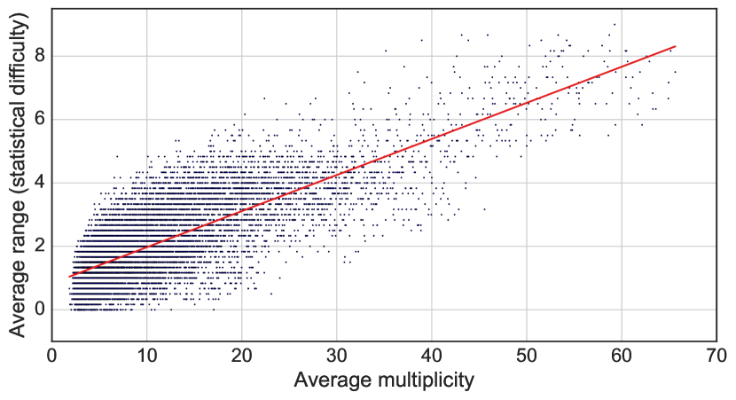
Figure 4: Statistical difficulty by average multiplicity ($r=0.784$). A multiplicity of 10 indicates that, in the corresponding instances, a given symbol is shared by an average of 10 tiles. For these instances, the average range of pagination sizes produced by our different solvers (the so-called difficulty) varies between 0 (all solvers obtain the same number of pages) and 5.

Figure 4 tests this hypothesis on our instance set: the average multiplicity of a given random instance appears to be a good predictor ($r=0.784$) of its statistical difficulty. Is it the best one? We can think of a few other possible candidates, and calculate their correlation with the statistical difficulty:

• $r=-0.082$ for $|\mathcal{A}|$, the number of symbols;

• $r=0.366$ for $|\mathcal{A}|\times|\mathcal{T}|$, the size of the instance, i.e., the number of bits required to encode it. More precisely, a stream of $|\mathcal{A}|\times|\mathcal{T}|$ bits, where the $i$th bit is 1 if and only if the $\lfloor i/|\mathcal{T}|\rfloor$-th tile of $\mathcal{T}$ includes the $(i\mod|\mathcal{T}|)$-th symbol of $\mathcal{A}$ (plus three long integers for the capacity, the size of the alphabet and the number of tiles, all of them being dominated by the first quantity).

• $r=0.563$ for $|\mathcal{T}|$, the number of tiles.

• $r=0.770$ for $\mathrm{Card}(\mathcal{T})$, the sum of the tile sizes.

Among these candidates, $\mathrm{Card}(\mathcal{T})$, the cardinality of the tile set, is almost as good a predictor as $\mathrm{Card}(\mathcal{T})/|\mathcal{A}|$, its average multiplicity. The choice of the latter value is mainly dictated by the fact that it involves the number of symbols. Indeed, when $|\mathcal{A}|$ approaches $\mathrm{Card}(\mathcal{T})$, Pagination approaches Bin Packing, which we expect to reduce the difficulty of the instance.

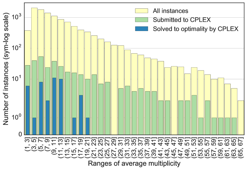
Figure 5: Number of instances by average multiplicity (sym-log scale).

Before we go any further, it is important to be aware that the average multiplicities in our test set are far from being evenly distributed (Fig. 5): for example, there are 1119 instances whose average multiplicity lies between 4 and 5, but only 107 between 23 and 24, and 10 between 53 and 54 (see [9] for these exact values). Overall, more than half of them concentrate between multiplicities 2 and 9. Thus, any observation made on the higher multiplicities (and the smaller ones) must be approached with great caution.

4.4 Discussion

4.4.1 Behavior of the integer linear program

As seen in Fig. 5, only a limited subset of our instances (342 of 10,986) have been submitted to CPLEX. This was for practical reasons: despite a powerful testing environment (Linux Ubuntu 12.04 on Intel Core i5-3570K with 4 cores of 3.4 GHz and 4 GB of RAM), CPLEX turned out to need a generous time-limit of one hour to be able to solve to optimality a mere 12.6 % of this subset (i.e., 43 instances). The ratio dropped to 3.8 % when the average multiplicity reached 13; above 20, no more success was recorded. Thus, this ILP quickly becomes irrelevant as the multiplicity increases, i.e., as Pagination starts to distinguish itself from Bin Packing.

Unless we could find strong valid inequalities to improve it, our experimentations suggest that the heuristic approach constitutes a better alternative.

4.4.2 Comparison of the heuristic methods

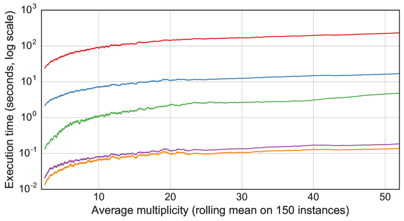
Figure 6: Performance of the main heuristics (log scale). From top (slowest) to bottom (fastest): Grouping GA, Standard GA, Overload-and-Remove, Best Fusion, First Fit.

All of our heuristics have been implemented in Python 2.7, and tested under Mac OS X 10.10 on Intel Core i5-3667U with 2 cores of 1.7 GHz and 4 GB RAM. The average execution time ranges from less than 0.1 seconds for the greedy algorithms, 1 second for Overload-and-Remove, 7 seconds for Standard GA, through 90 seconds for Grouping GA. For the two GAs, the following parameters were selected as offering the best ratio quality/time: 80 individuals, 50 generations, crossover rate of 0.90, mutation rate of 0.01. Their initial population was constituted of valid paginations obtained by applying First Fit to random permutations of the tile set. Figure 6 shows how the various algorithms scale as multiplicity grows: performance-wise at least, all remain practical on our most difficult instances.

Note that this analysis, and the next one, are carried out on a moving window of equally-sized subsets of instances sorted by increasing average multiplicity: by eliminating noise, this technique helps to visually separate the different curves; it has the side-effect of making some endpoints disappear, but, as explained in Section 4.3, their loss is greatly outweighed by the gain of a constant confidence level on the remaining data.

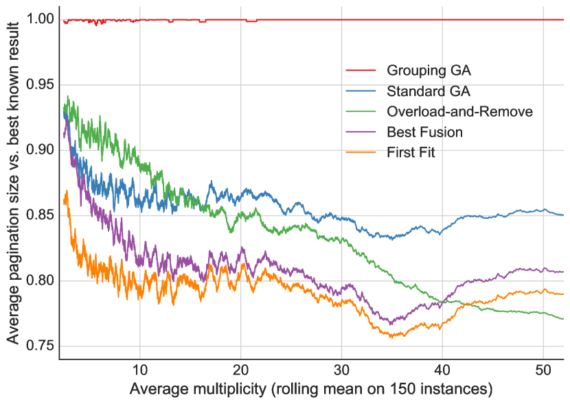
Figure 7: Relative quality of the five main heuristics. The outcomes are plotted at $y=\frac{\mathrm{best~{}size}}{\mathrm{size}}$, with $y=1$ corresponding to the best known solution (which is either the optimal or the best feasible solution found by CPLEX, or the smallest approximation calculated for the given instance).

Figure 7 compares the results of the various heuristics. The irregularities of the top line also somehow give indirect insight into the rare achievements of our ILP (among the 342 instances submitted to CPLEX, only 6 proved to have a better solution than the result of the best heuristic). General observations and recommendations that can be derived from the underlying data are as follows.

Standard GA can definitely be ruled out

As expected from Section 3.4.2, Standard GA was consistently surpassed by the more sensible Grouping GA: no more than 4 exceptions (0.036 %) occurred. Rather suspiciously, all of them involved a minimal instance, i.e., subject to a 2-page pagination. Further examination revealed that, in each case, this optimal pagination was already present in the initial random population constructed by First Fit; hence, its apparition was by no means indicative of some rare small-scale superiority of Standard GA: due to the fact that our implementation systematically transmits the best individual to the next generation, it was preserved, rather than produced by the evolution. This may also partially explain as pure chance the comparatively good performances in the lowest multiplicities; beyond that, the curve stabilizes quickly around an 85 % efficiency of Grouping GA. Finally, note that, up to an average multiplicity of 15, Standard GA is even outclassed by Overload-and-Remove, a six times faster heuristic.

Grouping GA produces the best overall results

When quality is the top priority, Grouping GA is the way to go: it almost always (99.64 % of cases) guarantees equivalent or smaller paginations than any other heuristic. ILP did improved on it in 6 cases (1.75 % of the 342 selected instances): 2 with a better feasible solution, 4 with the optimal solution. But even if such good surprises would multiply on the whole set of instances, we must keep in mind that CPLEX was given one hour on four cores, against about 90 seconds to a pure Python implementation running on a single core (twice as slow): Grouping GA has yet to unleash its full potential.

The fastest non-genetic contender is among Best Fusion and Overload-and-Remove

If speed matters, the choice depends on the average multiplicity of the instance: in most cases, Overload-and-Remove records quite honorable results. It is even the only non-genetic algorithm which proved occasionally (0.2 % of cases) able to beat Grouping GA. However, its quality regularly deteriorates (count up to 5 % for a 10 points increase in multiplicity). Around 35, somewhat surprisingly, the greedy algorithms get more and more competitive, with Best Fusion taking over at 40. Regardless of why this happens, a specialized heuristic for such deeply intricate instances would certainly be needed; in the meantime, Best Fusion represents the best tradeoff when average multiplicity meets or exceeds the 40 mark.

5 Conclusion

In this paper, we revisited an extension of Bin Packing originally devised by Sindelar et al. [19] for the virtual-machine colocation problem. We broadened its scope to an application-agnostic sharing model: in Pagination, two items can share unitary pieces of data, or symbols, in any non-hierarchical fashion. We showed that with such overlapping items, or tiles, the familiar tools and methods of Bin Packing may produce surprising results: for instance, while the family of Any Fit approximations have no more guaranteed performance, genetic algorithms still behave particularly well in the group-oriented encoding of [7]. We tested all these algorithms on a large set of random instances, along with an ILP solver, and some specialized greedy and non-greedy heuristics. The choice of the best one is not clear-cut, but depends on both time/quality requirements and the average multiplicity of the symbols. The latter measure was proposed as a predictor of the statistical difficulty of a given instance, and correlated experimentally with the actual outcome of our various algorithms.

Obviously, this work did not aim to close the problem, but rather to open it to further research, by providing the required vocabulary, several theoretical tools, and an extensive benchmark. Indeed, numerous directions should be investigated: examples of these are worst-case analysis, proof of lower bounds, elaboration of efficient cuts, etc. To make Pagination more manageable, a promising approach restricts it to one single page [8, 17].

References

- [1] Claude Berge. Graphs and Hypergraphs. Elsevier Science Ltd., Oxford, UK, UK, 1985.
- [2] Edward G. Coffman, Jr., Michael R. Garey, and David S. Johnson. Approximation algorithms for bin packing: a survey. In Dorit S. Hochbaum, editor, Approximation algorithms for NP-hard problems, chapter 2, pages 46–93. PWS Publishing Co., Boston, MA, USA, 1997.
- [3] Edward G. Coffman Jr., János Csirik, Gábor Galambos, Silvano Martello, and Daniele Vigo. Bin Packing Approximation Algorithms: Survey and Classification, pages 455–531. Springer New York, New York, NY, 2013.
- [4] György Dósa and Jiří Sgall. First Fit bin packing: A tight analysis. In 30th International Symposium on Theoretical Aspects of Computer Science (STACS 2013), volume 20, pages 538–549, Dagstuhl, Germany, 2013.
- [5] Mitre C. Dourado, Fabio Protti, and Jayme L. Szwarcfiter. Complexity aspects of the Helly property: Graphs and hypergraphs. The Electronic Journal of Combinatorics, #DS17:1–53, 2009.
- [6] John Duncan and Lawrence W. Scott. A branch-and-bound algorithm for pagination. Operations Research, 23(2):240–259, 1975.
- [7] Emanuel Falkenauer and Alain Delchambre. A genetic algorithm for bin packing and line balancing. In Proceedings of the 1992 IEEE International Conference on Robotics and Automation, pages 1186–1192, 1992.
- [8] Aristide Grange, Imed Kacem, Karine Laurent, and Sébastien Martin. On the Knapsack Problem Under Merging Objects’ Constraints. In 45th International Conference on Computers & Industrial Engineering 2015 (CIE45), volume 2, pages 1359–1366, Metz, France, 2015.
- [9] Aristide Grange, Imed Kacem, and Sébastien Martin. Algorithms for the bin packing problem with overlapping items: Dataset and experimental results. https://github.com/pagination-problem/pagination.
- [10] M. T. Hajiaghayi, K. Jain, K. Konwar, L. C. Lau, I. I. Măndoiu, A. Russell, A. Shvartsman, and V. V. Vazirani. The minimum -colored subgraph problem in haplotyping and DNA primer selection. In Proc. Int. Workshop on Bioinformatics Research and Applications, 2006.
- [11] David S. Johnson. Near-Optimal Bin Packing Algorithms. PhD thesis, Massachusetts Institute of Technology, Cambridge, 1973.
- [12] George Karypis and Vipin Kumar. Multilevel k-way Hypergraph Partitioning. In Proceedings of the 36th annual ACM/IEEE Design Automation Conference, DAC ’99, pages 343–348, New Orleans, Louisiana, USA, 1999. ACM.
- [13] Michael Kaufmann, Marc Kreveld, and Bettina Speckmann. Graph Drawing: 16th International Symposium, GD 2008, Heraklion, Crete, Greece, September 21-24, 2008. Revised Papers, chapter Subdivision Drawings of Hypergraphs, pages 396–407. Springer Berlin Heidelberg, Berlin, Heidelberg, 2009.
- [14] Krista Lagus, Ilkka Karanta, and Juha Ylä-Jääski. Paginating the generalized newspapers — A comparison of simulated annealing and a heuristic method, pages 594–603. Springer Berlin Heidelberg, Berlin, Heidelberg, 1996.
- [15] Silvano Martello and Paolo Toth. Bin-packing problem, pages 221–245. Wiley-Interscience series in discrete mathematics and optimization. J. Wiley & Sons, 1990.
- [16] Karl Pearson. Notes on regression and inheritance in the case of two parents. In Proceedings of the Royal Society of London, volume 58, pages 240–242, 1895.
- [17] Safraz Rampersaud and Daniel Grosu. A sharing-aware greedy algorithm for virtual machine maximization. In IEEE 13th International Symposium on Network Computing and Applications, NCA 2014, pages 113–120, 2014.
- [18] Safraz Rampersaud and Daniel Grosu. Sharing-aware online virtual machine packing in heterogeneous resource clouds. IEEE Transactions on Parallel and Distributed Systems, 2016. DOI 10.1109/TPDS.2016.2641937, 14 pages, to appear.
- [19] Michael Sindelar, Ramesh K. Sitaraman, and Prashant Shenoy. Sharing-aware algorithms for virtual machine colocation. In Proceedings of the 23rd ACM symposium on Parallelism in algorithms and architectures, pages 367–378, New York, New York, USA, 2011. ACM Press.
- [20] Emanuel Sperner. Ein satz über untermengen einer endlichen menge. Mathematische Zeitschrift, 27(1):544–548, 1928.
- [21] Apostolos Syropoulos. Mathematics of Multisets. Multiset Processing SE - 17, 2235(August):347–358, 2001.
- [22] David Wilcox, Andrew W. McNabb, and Kevin D. Seppi. Solving virtual machine packing with a reordering grouping genetic algorithm. In IEEE Congress on Evolutionary Computation, pages 362–369. IEEE, 2011.