Front propagation into unstable states in discrete media

Abstract

Non-equilibrium dissipative systems usually exhibit multistability, leading to the presence of propagative domain between steady states. We investigate the front propagation into an unstable state in discrete media. Based on a paradigmatic model of coupled chain of oscillators and populations dynamics, we calculate analytically the average speed of these fronts and characterize numerically the oscillatory front propagation. We reveal that different parts of the front oscillate with the same frequency but with different amplitude. To describe this latter phenomenon we generalize the notion of the Peierls-Nabarro potential, achieving an effective continuous description of the discreteness effect.

1 Introduction

Macroscopic systems under the influence of injection and dissipation energy, momenta, or matter usually exhibit coexistence of different states—this feature is usually denominated multistability [1, 2]. Inhomogeneous initial conditions, usually caused by the inherent fluctuations, generate domains that are separated by their respective interfaces. These interfaces are known as front solutions, interfaces, domain walls or wavefronts [2, 3, 4], depending on the physical context where they are considered. Interfaces between these metastable states appear in the form of propagating fronts and give rise to rich spatiotemporal dynamics [5, 6, 7]. Front dynamics occurs in systems as different as walls separating magnetic domains [8], directed solidification processes [6], nonlinear optical systems [9, 10, 11, 12], oscillating chemical reactions [13], fluidized granular media [14, 15, 16, 17], and population dynamics [18, 19, 20], to mention a few.

In one spatial dimension—from the point of view of dynamical systems theory—a front is a nonlinear solution that is identified in the co-moving frame system as a heteroclinic orbit linking two steady states [21, 22]. The evolution of front solutions can be regarded as a particle-type one, i.e., they can be characterized by a set of continuous parameters such as position, core width and so forth. The front dynamics depends on the nature of the steady states that are connected. In the case of a front connecting two stable uniform states, a variational system tends to minimize its energy or Lyapunov functional. Thus, the front solution always propagates with a well defined unique speed towards the less energetically favorable steady state. There is only one point in the parameter space for which the front is motionless, the Maxwell point. In systems with only local interaction between adjacent neighbors—a discrete medium—the front solutions persist [23, 24]. Once more, the most favorable state invades the less favorable one, being now the speed oscillatory. Actually, there is a region of the parameter space, close to the Maxwell point—the pinning range—where the fronts are motionless [24]. These properties can be explained by considering a potential for the front position, the Peierls-Nabarro barrier [25], which it is a result of the discreteness of the system.

The former scenario changes drastically for a front connecting a stable and an unstable state, usually called Fisher-Kolmogorov-Petrosvky-Piskunov (FKPP) front [18, 26, 27]. FKPP fronts have been observed in auto-catalytic chemical reaction [28], Taylor-Couette instability [29], Rayleigh-Benard experiments [30], pearling and pinching on the propagating Rayleigh instability [31], spinodal decomposition in polymer mixtures [32], and liquid crystal light valves with optical feedback [11]. One of the features of these fronts is that their speed is determined by initial conditions. When initial conditions are bounded, after a transient period, two counter propagative fronts emerge with the minimum asymptotic speed [18, 26, 27]. In discrete media, FKPP fronts also persist exhibiting an oscillatory behavior, however, the pinning phenomenon no longer exists. Beyond that, there is few understanding about their general behavior in discrete systems in our knowledge.

The aim of this article is to investigate, theoretically and numerically, the FKPP front propagation in discrete media. Based on paradigmatic models: the dissipative Frenkel-Kontorova and the discrete Fisher-Kolmogorov-Petrosvky-Piskunov equation. We determine analytically the minimum mean speed of FKPP fronts as a function of the medium discreteness. Numerically we characterize the oscillatory front propagation. We reveal that the front behaves as an extended object. Different parts of the front oscillate with the same frequency but with different amplitude. To describe this phenomenon we generalize the notion of the Peierls-Nabarro potential, which allows us to have an effective continuous description of the discreteness effect.

2 Chain of dissipative coupled pendula

Let us consider a chain of dissipative coupled pendula, known as the dissipative Frenkel-Kontorova model,

$$\ddot{\theta}_{i}=-\omega^{2}\sin\theta_{i}-\mu\dot{\theta}_{i}+\frac{\theta_{i+1}-2\theta_{i}+\theta_{i-1}}{dx^{2}},$$ (1)

where ${\theta}_{i}(t)$ is the angle formed by the pendulum and the vertical axis in the $i$-position at time t, $i$ is the index label the $i$-th pendulum, $\omega$ is the pendulum natural frequency, $\mu$ accounts for the damping coefficient, and $dx$ stands for the interaction between adjacent pendulums. This last parameter controls the degree of discreteness of the system. When $dx\to 0$ the system describes front propagation in a continuous medium, the dissipative sine-Gordon equation. In the conservative or Hamiltonian limit, $\mu=0$, the above equation is known as the Frenkel-Kontorova model, which describes the dynamics of a chain of particles interacting with the nearest neighbors in the presence of an external periodic potential. The Frenkel-Kontorova model, Eq. (1), is a paradigmatic model with application to several physical contexts. It has been used to describe the dynamics of atoms and atom layers adsorbed on crystals surfaces, incommensurate phase in dielectric, domain wall in magnetic domain, fluxon in Josephson transmission lines, rotational motion of the DNA bases, and plastic deformations in metals (see textbook [25] and references therein).

Note that equation (1) can rewrite in the following manner

$$\mu\dot{\theta}_{i}=-\frac{\delta F}{\delta\theta_{i}},$$ (2)

where the Lyapunov functional $F$ has the form

$$F\equiv\sum_{i=0}^{N}\left[\frac{\dot{\theta}_{i}^{2}}{2}-\omega^{2}\cos\theta_{i}+\frac{(\theta_{i+1}-\theta_{i+1})^{2}}{2dx^{2}}\right].$$ (3)

Hence, the dynamics of Eq. (1) is characterized by the minimization of functional $F$ when $\mu\neq 0$.

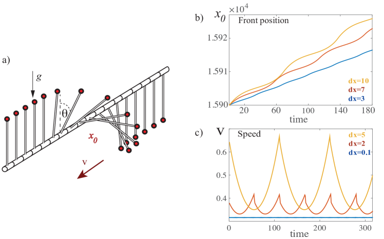
Figure 1: (color online) Chain of dissipative coupled pendula. a) Schematic representation of a chain of dissipative coupled of pendula. b) Temporal evolution of the front position $x_{0}(t)$ with $\omega=1$ and $\mu=20$. The upper (yellow), middle (orange) and lower (blue) lines correspond to $dx=10$, $dx=7$, and $dx=3$, respectively. c) Temporal evolution of the front speed $\dot{x}_{0}(t)$ with $\omega=1$ and $\mu=6$ . The upper (yellow), middle (orange) and lower (blue) lines correspond to $dx=5$, $dx=2$, and $dx=0.1$, respectively.

2.1 Propagation of a $\pi$-kink in a dissipative chain of pendula

In the range $\{0,2\pi\}$, Eq. (1) has steady states $\theta_{0}=0$ and $\theta_{1}=\pi$, which corresponds to the upright and upside-down position of pendulum, respectively. The upright (upside-down) position of the pendulum is a stable (unstable) equilibrium. Hence, the chain of dissipative coupled pendula can exhibits domains of upright or upside-down pendula as an extended state and a domain wall or connective front between both domains. This solution is usually denominated as a $\pi$-kink. Figure 1a illustrates a $\pi$-kink solution of this chain. The position of the domain wall, $x_{0}(t)$, is defined by a spatial location that interpolates a horizontal pendulum (cf. Fig. 1a). Due to coupling between pendulums, the domain wall propagates into the unstable state. Figures 1b and 1c show, respectively, front position and speed for different values of discreteness obtained from numerical simulations of equation (1). Numerical simulations were conducted using finite differences method with Runge-Kutta order-4 algorithm and specular boundary conditions. Indeed, the speed of propagation of the $\pi$-kink is oscillatory with a well defined average speed, $\langle v\rangle$. Unexpectedly, when discreteness $dx$ increases, the mean speed, amplitude and frequency of oscillation increases. Note that the oscillations exhibited by the speed are non-harmonic. Figure 2a shows the mean speed as function of the discreteness. For large discreteness, the speed increases linearly.

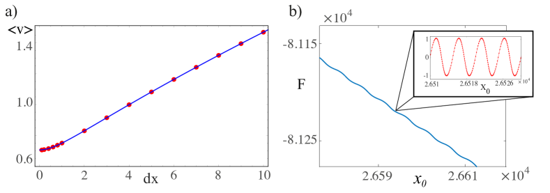
Figure 2: Front propagation into an unstable state in discrete chain of dissipative coupled pendula. a) Mean front speed as a function of the coupling parameter. Dots (red) are obtained by means of numerical simulations of Eq. (1) with $\omega=1.0$, $dx=5.0$ and $\mu=2.0$. The solid line is obtained by using the formulas (25) and (26). b) Lyapunov functional as function of front position obtained by numerical simulations of Eq. (1) for the same parameters. Inset: Lyapunov functional computed in the co-mobile system.

From a numerical solution of a chain of dissipative coupled pendula, we have computed the Lyapunov functional. Figure 2b shows evolution of the Lyapunov functional as a function of the front position $x_{0}$. As a matter of fact, the Lyapunov functional decreases with time in an oscillatory manner. It is clear from this results that the observed dynamical behavior is a consequence of the discreteness of the system.

To assess the above proposition we shall consider first a minimal theoretical model—the discrete Fisher-Kolmogorov-Petrosvky-Piskunov equation—that contains the main ingredients: coexistence between a stable and unstable state in a discrete medium.

3 The Discrete Fisher-Kolmogorov-Petrosvky-Piskunov model

Before study the effects of the discreteness in the FKPP-front, we shall establish some well-known facts about the front propagation into unstable states in the continuous case.

3.1 The Fisher-Kolmogorov-Petrosvky-Piskunov model: continuos medium

The most simple model that present front propagation into an unstable state is the Fisher-Kolmogorov-Petrosvky-Piskunov equation,

$$\partial_{t}u=u(1-u)+\partial_{xx}u,$$ (4)

where $u(x,t)$ is an order parameter that accounts for an extended transcritical bifurcation. The above model was used to study the populations dynamics in several contexts [18], where the main ingredients are linear growth, nonlinear saturation (logistic nonlinearity), and Fickian transport process.

In this model, $u=0$ is an unstable fixed point and $u=1$ is a stable one. If the initial conditions have compact support, i.e., $u(x,0)=u_{0}(x)$ with

$$u_{0}(x)=\left\{\begin{array}[c]{c}0,\text{ \ \ \ }x<x_{1}\\ f(x),\text{ \ \ \ \ }x_{1}\leq x\leq x_{2}\\ 0,\text{ \ \ \ }x<x_{2}\end{array}\right.$$ (5)

where $f(x)$ is a positive and bounded function, the solution $u(x,t)$ will evolve to a two counter propagating front solutions, which propagate to speed $v=2$. In other words, the fronts move with minimum speed $v_{min}=2$ [26, 27]. This speed was determined by considering traveling solutions in the co-mobile dynamical system. After, we perform a linear analysis around the unstable state, imposing that the front solutions do not exhibit damped spatial oscillations [26]. Henceforth, we shall denominate this method to determine the minimum speed as FKPP procedure. This result was obtained in the pioneering work of Luther [28], in the context of wave propagation in catalytic chemical reaction. As this minimum speed is determined by means of a linear analysis it is usually called linear criterion. This linear criterion for the determine the minimum speed of front propagation into unstable states is valid for weakly nonlinearity, as it is established in the work of Kolmogorov et al. [26] (for more details see Rev. [27] and references therein). For strong nonlinearity, nonlinear criterion, the front propagation into unstable states also have a minimum speed, however there is no general formulation to determine the value of such speed. For gradients equations have been developed a variational method to determine an adequate approximation to the minimum speed [33]. Fronts whose minimum speed is determined by the linear or nonlinear criteria are usually called pulled or pushed front, respectively [27].

As we have mention for different initial conditions, the front solution will strongly depend of the asymptotic behavior of $u(x,0)$ for $x\to\pm\infty$. Considering an initial conditions of the form $u(x,0)\sim Ae^{-kx}$ for $x\to\infty$ where $\{k,A\}$ are positive constants. The front propagates as a wave of the form $u(x,t)=u\left(k(x-vt)\right)$. Linearizing Eq. (4) and considering $u(x,t)\sim Ae^{-k(x-vt)}$ for $x\to\infty$, after straightforward calculations one can obtain the following relation [39],

$$v=\frac{1}{k}+k.$$ (6)

Thus, $v$ as function of $k$ is a convex function. Minimizing the previous curve with respect to $k$, we obtain the critical steepness $k\equiv k_{c}=1$, for which we obtain the minimal speed $v(k_{c})\equiv v_{min}=2$. This method is the asymptotic process. For any other value of the steepness $k$ the front propagates with a speed larger than $v_{min}$ ($v(k)\geqslant v_{min}$). Hence, using the asymptotic shape of the front solution one can determine the minimum speed, when the linear criterion is valid. Note that this procedure can only determine the minimum speed of a pulled front. It is noteworthy to mention that the asymptotic solution for all co-mobile reference systems, i.e., $z=x-vt$ is [38]

$$u(z)=\frac{1}{\left(1+e^{z/v}\right)}+\frac{1}{v^{2}}\frac{e^{z/v}}{\left(1+e^{z/v}\right)^{2}}\ln\left[\frac{4e^{z/v}}{\left(1+e^{z/v}\right)^{2}}\right]+\mathcal{O}\left(\frac{1}{v^{4}}\right)$$ (7)

where $v\geq v_{min}=2$.

3.2 Front propagation in discrete FKPP model

Let us consider a simple discrete version of the Fisher-Kolmogorov-Petrosvky-Piskunov model, Eq.(4),

$$\dot{u}_{i}=u_{i}(1-u_{i})+\frac{u_{i+1}-2u_{i}+u_{i-1}}{dx^{2}},$$ (8)

where $u_{i}(t)$ stands for the population in $i$-th position. It is assumed that locally the growth is linear, the saturation is nonlinear, and that the population flow is proportional to the population difference of near neighbors. Note that the dynamics of discrete FKPP model can rewrite in the following form

$$\partial_{t}u_{i}=-\frac{\partial{\cal F}}{\partial u_{i}}$$ (9)

where the Lyapunov function is defined as

$${\cal F}=\sum_{i}\left(-\frac{u_{i}^{2}}{2}+\frac{u_{i}^{3}}{3}+\frac{(u_{i+1}-u_{i})^{2}}{2\,dx^{2}}\right)=\sum_{i}V_{i}+\frac{(u_{i+1}-u_{i})^{2}}{2\,dx^{2}},$$ (10)

where $V_{i}$ is the potential. Hence, the dynamics of Eq. (8) is characterized by the minimization of functional $F$. Indeed, using Eq. (8), one obtains

$$\frac{d{\cal F}}{dt}=\sum_{i}\frac{\partial{\cal F}}{\partial u_{i}}\frac{\partial u_{i}}{\partial t}=-\sum_{i}\left(\frac{\partial{\cal F}}{\partial u_{i}}\right)^{2}.$$ (11)

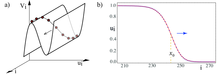
Figure 3: (color online) Front solution of the FKKP model Eq. (8). a) Schematic representation of potential $V_{i}$. b) Front solution obtained numerically from Eq. (8) (blue dots) and the asymptotic solution Eq.(7) (solid line); $x_{0}$ accounts for the front position.

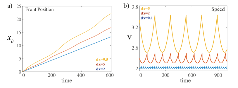
Figure 4: (color online) Front propagation into an unstable state in discrete FKPP Eq. (8). a) Temporal evolution of front position $x_{0}(t)$. The upper (yellow), middle (orange) and lower (blue) lines correspond to $dx=9.5$, $dx=5$, and $dx=2$, respectively. b) Temporal evolution of front speed $\dot{x}_{0}(t)$. The upper (yellow), middle (orange) and lower (blue) lines correspond to $dx=5$, $dx=2$, and $dx=0.1$, respectively.

The discrete Fisher-Kolmogorov-Petrosvky-Piskunov Eq. (8) exhibits front propagation into an unstable state. In Ref.[40], it has been established the existence of these solutions, however their oscillatory propagation has not been yet characterized. Figure 3 shows a schematic representation of potential $V_{i}$ and the front solution. From this figure, one trivially deduces the energy source of the front propagation.

Defining the front position as the spatial position that interpolate the maximum spatial gradient, $u(x_{0})=1/2$ (cf. Fig. 3b), one can study the front propagation. Figure 4 shows, respectively, the front position and minimum speed for different values of discreteness obtained from numerical simulations of model Eq. (8). We can observe similar dynamical behavior that those exhibit by a chain of dissipative coupled pendula (cf. Fig. 1), that is, the front propagates with an oscillatory speed with a given mean speed. When coupling parameter $dx$ increases, the mean speed, amplitude and frequency of oscillations increases. Moreover, the oscillations exhibited by the speed are non-harmonic type. Figure 5a shows the mean speed as a function of the coupling parameter. For large $dx$ the speed increases linearly.

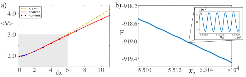
Figure 5: (color online) Front propagation into an unstable state in FKPP model, equation (8). a) Minimum mean speed as a function of the discreteness $dx$. Dots (blue) correspond to numerical simulations of model (8). The solid (red) and dashed (yellow) lines are the exact and approximative curve obtained form expressions (18) and (21), respectively. b) Lyapunov functional as a function of front position obtained from numerical simulations of Eq. (8) with $dx=10$. Inset: Lyapunov functional computed in the co-mobile system.

From a numerical solution of FKPP model Eq. (8), we have computed the Lyapunov functional (10). Figure 5b shows evolution of Lyapunov functional as a function of the front position. In the inset of Fig. 5b, we show the Lyapunov functional in the co-mobile system. As we can see, Lyapunov functional decreases with time in a oscillatory manner.

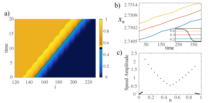
Figure 6: Front propagation into an unstable state in discrete FKPP model (8). a) Spatiotemporal evolution of the front propagation into an unstable state in discrete FKPP model (8) with $dx=7.5$. b) Trajectory of three different points or cuts: Above (upper yellow line), in (middle red line), and below (lower blue line) the front position. Inset illustrates different cuts under consideration. c) Oscillation amplitude of the front speed in different points.

Usually, the study of the front dynamics is reduced to the front position, i.e., the dynamical tracking of point $x_{0}$, where $u(x_{0})=1/2$ is the maximum of the spatial gradient. This is based on the assumption that the front behaves as a point-like particle. Thus, point $x_{0}$ will gives us enough information about the whole structure dynamics. Surprisingly, the FKPP front exhibits an extended object behavior: each point of the front shows an oscillation dynamics with the same frequency but different amplitude. Figure 6a shows the spatiotemporal diagram of the front. From this figure, is easy to infer that the front propagates as an extended object. Moreover, the oscillation with respect to front position $x_{0}$ are in anti-phase (see Fig. 6b). That is, the maximum oscillation of a point to the left of the front position coincides with the minimum oscillation of a point to the right. To explore the structure of the potential over which the front propagates, we have followed different points or ”cuts” along the front profile, studying each one separately. Figure 6c displays the amplitude of oscillation of the front speed for different cuts. From this figure, we conclude that this amplitude is minimal at the front position, increases as one moves away from the front position and decays to zero abruptly in the front tails.

3.3 Theoretical description of the mean speed for the discrete FKPP model

For discrete media, the FKPP procedure is unsuitable to determine the minimum speed. Due to there is not a continuos dynamical system associated to the co-mobile system inferred for traveling wave solutions. To compute the minimal front speed, we generalize the asymptotic procedure ansatz for the front tail [39],

$$u_{i}(t)=e^{\left(\alpha t-2i\beta\right)}\left[1+f_{dx;i}^{\omega}(t)\right],\quad\quad\quad i\gg 1,$$ (12)

with $\alpha\equiv k\langle v\rangle$ and $\beta\equiv k\,dx/2$ are parameters. The index $i\geq 0$ is a positive and large integer number, $dx$ is the discretization parameter, $\langle v\rangle$ is the mean speed of the front, and $f_{dx,i}^{\omega}(t)$ is a time periodic function with period $T\equiv 2\pi/\omega$, i.e., $f_{dx;i}^{\omega}(t)=f_{dx;i}^{\omega}(t+T)$, which accounts for the oscillation of the front speed at the $i$-th position (cf. Fig. 6). In addition, $f_{dx;i}^{\omega}(t)\to 0$ when $i\to\infty$. Hence, function $f_{dx,i}^{\omega}(t)$ takes into account the periodicity introduced by the discreteness. Linearizing discrete FKKP model (8) and replacing ansatz (12), we get

$$\begin{split}\dot{u}_{i}&=\dot{f}_{dx;i}^{\omega}+\alpha\left[1+f_{dx;i}^{\omega}\right]\\ &=\left[1+f_{dx;i}^{\omega}\right]+\frac{k^{2}}{\beta^{2}}\left[\left(\sinh^{2}\left(\beta\right)\right)+\left(\sinh^{2}\left(\beta\right)\right)f_{dx;i}^{\omega}\right].\end{split}$$

Integrating this expression in a normalized period $T$

$$\langle\dot{f}_{dx;i}^{\omega}+\alpha\left[1+f_{dx;i}^{\omega}\right]\rangle=\langle\left[1+f_{dx;i}^{\omega}\right]+\frac{k^{2}}{\beta^{2}}\left[\left(\sinh^{2}\beta\right)+\left(\sinh^{2}\beta\right)f_{dx;i}^{\omega}\right]\rangle,$$ (13)

where

$$\langle g(t)\rangle\equiv\frac{1}{T}\int_{0}^{T}g(t)dt,$$ (14)

we obtain an expression for the mean speed $\langle v\rangle$

$$\langle v\rangle=\frac{1}{k}+k\left(\frac{\sinh\beta}{\beta}\right)^{2}.$$ (15)

with $\langle f_{dx;i}^{\omega}\rangle=\langle\dot{f}_{dx;i}^{\omega}\rangle=0$, due to $f_{dx;i}^{\omega}(t)$ periodicity. This expression accounts for the mean speed as a function of steepness and discreteness parameters. Note that $\langle v\rangle$ tends to expression (6) when $dx\to 0$ ($\beta\to 0$), which corresponds to the continuous limit. Figure 7 shows the mean speed as a function of the parameter $k$ for different values of the discretization parameter $dx$. For different values of discretization parameter $dx$, $\langle v\rangle$ is a concave function. We can observe, that the minimum speed $\langle v\rangle_{min}$ increases as the discretization parameter $dx$ grows. Meanwhile, the critical steepness $k_{c}$ decreases. By differentiating the mean speed relation (15) and equating to zero, we obtain an expression for the discretization parameter,

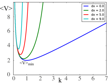
Figure 7: Mean speed $\langle v\rangle$ as a function of the steepness parameter $k$ for different values of the discretization parameter $dx$, formula (15). From the lower to upper curve we consider $dx=0,2,5$ and $9$, respectively.

$$dx^{2}=4\sinh\beta_{c}(2\beta_{c}\cosh\beta-\sinh\beta_{c}),$$ (16)

where $\beta_{c}=k_{c}dx/2$ and $k_{c}$ is the critical steepness to obtain the minimum speed. Replacing the definition of $\beta_{c}$ in above expression, we get

$$dx^{2}=4\sinh\left(\frac{k_{c}dx}{2}\right)\left[k_{c}dx\cosh\left(\frac{k_{c}dx}{2}\right)-\sinh\left(\frac{k_{c}dx}{2}\right)\right].$$ (17)

One can not explicitly determine the critical steepness as fa unction of discretization parameter $dx$, $k_{c}(dx)$. Hence, minimum speed as a function of $dx$ is a implicit formula

$$\langle v\rangle_{mim}=\frac{1}{k_{c}(dx)}+k_{c}(dx)\left(\frac{\sinh\beta(dx)}{\beta(dx)}\right)^{2}.$$ (18)

The continuos curve in Fig. 5a is the minimal mean speed as a function of the discretization, expression (18). Numerical simulations show quite good agreement with this expression (cf. Fig. 5a).

Figure 8: (color online) Parameter as function of discretization. a) Discretization as a function of $\beta$ parameter. Solid (blue) and dashed (yellow) lines are the exact and approximative analytic curves (17) and (19), respectively. b) Steepness $k$ as a function of the discretization parameter, $dx$. Solid and dashed lines are the exact and approximative analytic curves (17) and (20), respectively. Dots (blue) are obtained by numerical simulations.

To have an explicit analytical expression we consider the limit $\beta\to 0$, thus expression (19) can be simplified to

$$dx\approx 2\beta_{c}\sqrt{1+\beta_{c}^{2}}.$$ (19)

From here, we can write the parameter $\beta_{c}$

$$\beta_{c}\approx\frac{dx}{\sqrt{2\left(1+\sqrt{1+dx^{2}}\right)}}$$

and the critical steepness

$$k_{c}\approx\sqrt{\frac{2}{1+\sqrt{1+dx^{2}}}}$$ (20)

as a function of the discretization parameter $dx$. Figure 8 shows the discretization parameter $dx$ as a function of $\beta$ (Eq. (19)). The shadow area illustrates the limit where the approximation $\beta\to 0$ is valid. Likewise, figure (8) shows the steepness $k$ as a function of the parameter $dx$. From both, we can infer that expressions (19) and (20) are valid in a wide range of the parameter $dx$. Therefore, in a good approximation the mean speed $\langle v\rangle$ can take the form,

$$v\approx\sqrt{\frac{1+\sqrt{1+dx^{2}}}{2}}\left[1+\frac{4}{dx^{2}}\sinh^{2}\left(\frac{dx}{\sqrt{2\left(1+\sqrt{1+dx^{2}}\right)}}\right)\right].$$ (21)

Figure 5 shows the mean speed as a function of the discretization parameter $dx$. Up to a value of $dx=6.0$, expression (21) is an adequate approximation. We observe a good accordance between the analytic expression and the mean speed obtained by numerical simulations.

In brief, the asymptotic procedure allows an adequate characterization of the average features of front propagation into unstable states in discrete media. In the next section, we shall apply this procedure to characterize the mean properties of front propagation into unstable state in a chain of dissipative coupled pendula.

3.4 Theoretical description of the mean speed for the Chain of dissipative coupled pendula

For the chain of dissipative coupled pendula, Eq. (1), the unstable state correspond to $\theta_{i}=\pi/2$. Considering the asymptotic ansatz for the front tail around this state, we get,

$$\theta_{i}(t)=\frac{\pi}{2}+A_{0}e^{\left(\alpha t-2i\beta\right)}\left[1+f_{dx;i}^{\omega}(t)\right],$$ (22)

where $A_{0}$ is a constant that characterizes the shape of the front tail, $\alpha\equiv k\langle v\rangle$ and $\beta\equiv k\,dx/2$ are parameters. $f_{dx;i}^{\omega}(t)$ is a periodic function of frequency $\omega$ in $i$-th position of the chain that describes the oscillatory behavior of the speed. Introducing the above ansatz in Eq. (1) and taking into account only the linear leading terms, we obtain,

$$\begin{split}\ddot{\theta}_{i}&=\alpha^{2}\left[1+f_{dx;i}^{\omega}(t)\right]+2\alpha\dot{f}_{dx;i}^{\omega}(t)+\ddot{f}_{dx;i}^{\omega}(t)\\ &=\omega^{2}\left[1+f_{dx;i}^{\omega}(t)\right]-\mu\left[\alpha\left[1+f_{dx;i}^{\omega}(t)\right]+\dot{f}_{dx;i}^{\omega}(t)\right]+\frac{4}{dx^{2}}\sinh^{2}(\beta)\left[1+f_{dx;i}^{\omega}(t)\right]\end{split}$$

Integrating this expression in a normalized period $T=2\pi/\omega$, and considering $\langle f_{dx;i}^{\omega}(t)\rangle=\langle\dot{f}_{dx;i}^{\omega}(t)\rangle=\langle\ddot{f}_{dx;i}^{\omega}(t)\rangle=0$, after straightforward calculations, we obtain

$$\begin{split}\alpha^{2}=\omega^{2}-\mu\alpha+\frac{4}{dx^{2}}\sinh^{2}(\beta).\end{split}$$ (23)

Substituting the definition of $\alpha$, the mean speed reads

$$\langle v\rangle=-\frac{\mu}{k}+\frac{1}{k}\sqrt{\mu^{2}+\omega^{2}+\frac{k^{2}}{\beta^{2}}\sinh^{2}(\beta)},$$ (24)

and replacing $k=2\beta/dx$,

$$\langle v\rangle=-\frac{\mu}{2\beta}dx+\frac{1}{2\beta}\sqrt{dx^{2}\left(\mu^{2}+\omega^{2}\right)+4\sinh^{2}(\beta)}$$ (25)

The above expression accounts for front speed as a function of the steepness. In order to deduce the minimal front speed, we differentiate the above speed with respect to $\beta$

$$\begin{split}&\omega^{2}\left(\mu^{2}+\omega^{2}\right)dx^{4}+4\left[\left(\mu^{2}+2\omega^{2}\right)\sinh^{2}(\beta)-2\left(\mu^{2}+\omega^{2}\right)\beta\sinh(\beta)\cosh(\beta)\right]dx^{2}\\ &+16\sinh^{2}(\beta)\left[\sinh(\beta)-\beta\cosh(\beta)\right]^{2}=0.\end{split}$$ (26)

This expression gives us a relation between the critical steepness $k_{c}$ and the coupling parameter $dx$. An explicit expression $k_{c}(dx)$ cannot be derived. Using expression (26) in formula (25), we obtain the minimal front speed for the chain of dissipative coupled pendula, Eq (1). Note that this analytical results has quite fair agreement with the numerical simulations as it is shown in Fig. 2a. Therefore, the asymptotic procedure is a suitable method to characterize the mean properties of front propagation.

4 Effective continuous model: oscillatory properties of front propagation

Due to the complexity of discrete dissipative systems, to obtain analytical results is a daunting task. In order to figure out the oscillatory behavior of the front, we shall consider a similar strategy to that used in Ref. [24], which is based on considering an effective continuous equation that accounts for the dynamics of the discrete system. The benefit of this approach is that analytical calculations are accessible.

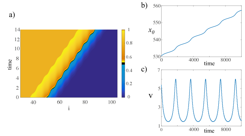
Figure 9: (color online) Front propagation into an unstable state in FKPP Eq. (29) with a harmonic generalized Peierls-Nabarro potential, $\Gamma_{dx}(x)=A\cos(2\pi x/dx)$ with $A=0.06$, and $dx=5.0$. The numerical discretization parameter of the finite differences method is $0.1$. a) Spatiotemporal evolution of the front propagation into unstable state. b) Temporal evolution of the front position and c) minimum speed.

4.1 Generalized Peierls-Nabarro potential

Let us consider the continuos order parameter $u(x,t)$, which satisfies

$$\partial_{t}u=-\frac{\delta{\cal F}}{\delta u},$$ (27)

where the Lyapunov functional has the form

$${\cal F}=\int\left(-\frac{u^{2}}{2}+\frac{u^{3}}{3}+\frac{(\partial_{x}u)^{2}}{2}+(\partial_{x}u)^{2}\Gamma_{dx}(x)\right)dx,$$ (28)

$\Gamma_{dx}(x)$ is a spatial periodic function with $dx$ period, $\Gamma_{dx}(x+dx)=\Gamma_{dx}(x)$. This function accounts for the discreteness of the system. The last term of the free energy is a generalization of the Peierls-Nabarro potential. An effective potential has been used to explain the dynamics of defects position such as dislocations in condensed matter physics or dynamics of the position of kink or fronts (see textbook [25] and reference therein). Here, we consider an effective equation for the entire field $u(x,t)$, which reads

$$\partial_{t}u=u(1-u)+D\partial_{xx}u+2\Gamma_{dx}(x)\partial_{xx}u+2\Gamma^{\prime}_{dx}(x)\partial_{x}u.$$ (29)

This equation is a populations dynamical model with linear growth, nonlinear saturation, inhomogeneous diffusion and drift force. Numerical simulations with a harmonic potential $\Gamma_{dx}$ exhibit front solutions. It is important to note that for these numerical simulations, we have discretized the Laplacian and gradient of $u$ to first neighbors considering a small $dx$. For which the discreteness effects are negligible. Figura 9 shows the spatiotemporal diagram of the front into an unstable state of the effective FKPP, Eq. (29), with a harmonic generalized Peierls-Nabarro potential. Its trajectory and speed are also illustrated. We can observe that the numerical simulations of the effective FKPP, Eq. (29), and discrete FKPP, Eq. (8), have similar qualitative dynamical behaviors.

To understand better the generalized Peierls-Nabarro potential, Figure 11a shows the effective force for the harmonic case and the amplitude speed for the effective FKPP Eq. (29). From this figure, we infer that the effective force, $f\equiv 2\Gamma_{dx}(x)\partial_{xx}u+2\Gamma^{\prime}_{dx}(x)\partial_{x}u$, has an oscillatory structure concentrated in the region where the front displays larger spatial variations. Moreover, we observe that the structure of the amplitude of the speed is similar to that observed in the discrete case (cf. Figs. 11b and 6c).

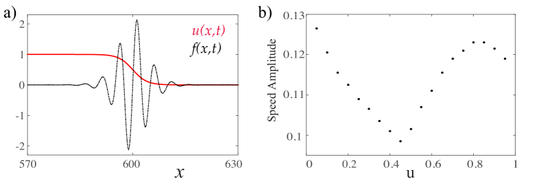
Figure 10: The generalized Peierls-Nabarro force for a harmonic case, $\Gamma_{dx}(x)=A\cos(2\pi x/dx)$. a) Front solution and effective force $f\equiv 2\Gamma_{dx}(x)\partial_{xx}u+2\Gamma^{\prime}_{dx}(x)\partial_{x}u$. b) Amplitude of the speed for the effective FKPP Eq. (29) with $D=1.97$, $A=0.03$, and $dx=5.0$. The numerical discretization parameter of the finite differences method is $0.1$.

4.2 Dynamics of front position

The equilibria are not affected by the presence of the periodical extra terms, effective force. In the continuous limit, $dx\to 0$ and $\Gamma_{dx}(x)\to 0$ one recovers the Fisher-Kolmogorov-Petrosvky-Piskunov model Eq. (4). Then for $dx\ll 1$, the last two terms of Eq. (29) are perturbative. We shall analyze this region of parameters, where we can obtain analytical results.

The Fisher-Kolmogorov-Petrosvky-Piskunov model Eq. (4) has front solutions of the form $u_{FKPP}(x-vt-p)$, where $p$ is a constant that accounts for the front position and $v$ the front speed. Analytical expressions of this solution are unknown, however solutions in the form of perturbative series are available [18]. Considering the following ansatz for small discreteness ($dx\ll 1$)

$$u(x,t)=u_{FKPP}\left(x-vt-p(t)\right)+w(x-vt-p(t),p(t)),$$ (30)

where front position is promoted to a temporal function, $p(t)$ and $w$ is a corrective function on the order of the perturbative force. Introducing the above ansatz in Eq. (29) and linearizing in $w$, after straightforward calculations, we obtain

$${\cal L}w=-\dot{p}(t)\partial_{\xi}u_{FKPP}-2\Gamma_{dx}(x)\partial_{\xi\xi}u_{FKPP}-2\Gamma^{\prime}_{dx}(x)\partial_{\xi}u_{FKPP},$$ (31)

where ${\cal L}\equiv\partial_{\xi\xi}+v\partial_{\xi}+1-2u_{FKPP}(\xi)$ is a linear operator and $\xi=x-vt-p$ is the coordinate in the co-mobile system. Considering the inner product

$$\left<f|g\right>=\int_{-L}^{L}f(\xi)g(\xi)d\xi,$$ (32)

where $2L$ is the system size. In order to solve the linear Eq. (31), we apply the Fredholm alternative or solvability condition [2], and obtain

$$\dot{p}(t)=-2\frac{\left<\Gamma_{dx}(\xi+vt+p)\partial_{\xi\xi}u_{FKPP}|\psi\right>}{\left<\partial_{\xi}u_{FKPP}|\psi\right>}-2\frac{\left<\Gamma^{\prime}_{dx}(\xi+vt+p)\partial_{\xi}u_{FKPP}|\psi\right>}{\left<\partial_{\xi}u_{FKPP}|\psi\right>},$$ (33)

where $\psi(\xi)$ is an element of kernel of adjoint of $\cal L$, ${\cal L^{\dagger}}\equiv\partial_{\xi\xi}-v\partial_{\xi}+1-2u_{FKPP}(\xi)$, that is ${\cal L}^{\dagger}\psi=0$. The $\psi$ function is unknown analytically, however the asymptotic behavior of this function are characterized to diverges exponentially with the the same exponent that $u_{FKPP}$ converges to their equilibria. Therefore the above integrals diverge proportional to $L$, however the ratio is well defined.

To understand the dynamics described by the above equation for simplicity we shall consider the generalized Peierls-Nabarro potential for a harmonic case, that is,

$$\Gamma_{dx}(x)=\gamma(x)\equiv A\cos\left(\frac{2\pi x}{dx}\right),$$ (34)

Replacing this expression in Eq. (33), after straightforward calculations, we obtain

$$\dot{p}(t)=\sqrt{K_{1}^{2}+K_{2}^{2}}\cos\left(\frac{2\pi}{dx}(p-vt)+\phi_{0}\right),$$ (35)

with

$$K_{1} = A\frac{\left<\cos\left(\frac{2\pi\xi}{dx}\right)\partial_{\xi\xi}u_{FKPP}(\xi)-\frac{2\pi\xi}{dx}\sin\left(\frac{2\pi\xi}{dx}\right)\partial_{\xi}u_{FKPP}|\psi(\xi)\right>}{\left<\partial_{\xi}u_{FKPP}|\psi(\xi)\right>},$$

$$K_{2} = -A\frac{\left<\sin\left(\frac{2\pi\xi}{dx}\right)\partial_{\xi\xi}u_{FKPP}(\xi)+\frac{2\pi\xi}{dx}\cos\left(\frac{2\pi\xi}{dx}\right)\partial_{\xi}u_{FKPP}|\psi(\xi)\right>}{\left<\partial_{\xi}u_{FKPP}|\psi(\xi)\right>},$$

$$\tan(\phi_{0}) = \frac{K_{1}}{K_{2}}.$$ (36)

Therefore, the front position propagates in a oscillatory manner. Notice that the Peierls-Nabarro potential propagates together with the front. Figure 11 shows fitting curve for $\dot{p}$ using solution of (35) if $\Gamma_{dx}(x)$ is given by (34). We can see that the analytical result is in good agreement with the observed dynamics.

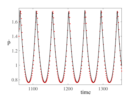
Figure 11: Fitting curve for $\dot{p}$ given by the expression $\ \dot{p}=\frac{a\sec^{2}(bx+c)}{1+\left(d\tan(bx+c)-e\right)^{2}}+f$ with $a=0.57$, $b=0.0682$, $c=0.6157$, $d=1$, $e=0.8$, and $f=0.5$

5 Conclusions and remarks

We have studied, theoretically and numerically, the front propagation into unstable states in discrete dissipative systems. Based on a paradigmatic model of coupled chain of oscillators (the dissipative Frenkel-Kontorova model) and population dynamic model (the discrete and effective Fisher-Kolmogorov-Petrosvky-Piskunov model), we have determined analytically the mean speed of FKPP fronts when nonlinearities are weak. Numerically we have characterized the oscillatory front propagation. Likewise, we have revealed that different parts of the front oscillate with the same frequency but with different amplitude. To describe this phenomenon, we have generalized the notion of the Peierls-Nabarro potential, which allows us to have an effective continuous description of discreteness effect.

The analysis presented only is valid for weak nonlinearity, where linear criterium is valid. The characterization of pushed front in local coupling dissipative systems is an open and relevant question. Propagation fronts in two dimensions is affected by the curvature of the interface, which can increase o decrease the speed of the propagating interface. Study of front propagation into unstable states in these contexts are in progress.

References

References

- [1] Nicolis G, Prigogine I. Self-Organization in Non Equilibrium Systems. New York: J. Wiley and Sons; 1977.
- [2] Pismen LM. Patterns and Interfaces in Dissipative Dynamics. Berlin Heidelberg: Springer Series in Synergetics; 2006.
- [3] Cross MC, Hohenberg PC. Pattern formation outside of equilibrium. Rev Mod Phys 1993;65:851.
- [4] Cross M, Greenside H. Pattern Formation and Dynamics in Nonequilibrium Systems. New York: Cambridge University Press; 2009.
- [5] Pomeau Y. Front motion, metastability and subcritical bifurcations in hydrodynamics. Physica D 1986;23:3.
- [6] Langer JS. Instabilities and pattern formation in crystal growth. Rev Mod Phys 1980;52:1.
- [7] Collet P, Eckman J. Instabilities and Fronts in Extended Systems. Princeton: Princeton University Press; 2014.
- [8] Eschenfelder AH. Magnetic Bubble Technology. Berlin Heidelberg: Springer; 1980.
- [9] Clerc MG, Residori S, Riera CS. First-Order Freedericksz transition in the presence of a light driven feedback. Phys Rev E 2001;63:060701.
- [10] Gomila D, Colet P, Oppo GL, San Miguel M. Stable droplets and growth laws close to the modulational instability of a domain wall. Phys Rev Lett 2001;87:194101.
- [11] Clerc MG, Nagaya T, Petrossian A, Residori S, Riera C. First-Order Fr edericksz Transition and Front Propagation in a Liquid Crystal Light Valve with Feedback. Eur Phys J 2004;28:435.
- [12] Residori S. Patterns, fronts and structures in a liquid-crystal-light-valve with optical feedback. Physics Reports 2005;416:201.
- [13] Petrov V, Ouyang Q, Swinney HL. Resonant pattern formation in a chemical system. Nature 1997;388:655.
- [14] Aranson I, Tsimring L. Granular Patterns. Oxford: Oxford University Press; 2008.
- [15] Douady S, Fauve S, Laroche C. Subharmonic instabilities and defects in a granular layer under vertical vibrations. Europhysics Letters 1989;8:621.
- [16] Moon SJ, Goldman DI, Swift JB, Swinney HL. Kink-induced transport and segregation in oscillated granular layers. Phys Rev Lett 2003;91:134301.
- [17] Macias JE, Clerc MG, Falcon C, Garcia-Nustes MA. Spatially modulated kinks in shallow granular layers. Phys Rev E 2013;88:020201.
- [18] Murray JD. Mathematical Biology. Berlin Heidelberg: Springer; 1989.
- [19] Fisher RA. The wave of advance of advantageous genes. Ann Eugenics 1937;7:353.
- [20] Clerc MG, Escaff D, Kenkre VM. Patterns and localized structures in population dynamics. Phys Rev E 2005;72:056217.
- [21] Saarloos W van, Hohenberg PC. Fronts, pulses, sources and sinks in generalized complex Ginzburg-Landau equations. Physica D 1992;56:303.
- [22] Coullet P. Localized patterns and fronts in nonequilibrium systems. Int J Bifurcation Chaos 2002;12:2445.
- [23] Fáth G. Propagation failure of traveling waves in a discrete bistable medium. Physica D 1998;116:176.
- [24] Clerc MG, Elías RG, Rojas RG. Continuous description of lattice discreteness effects in front propagation. Phil Trans R Soc A 2011;369:1.
- [25] Braun OM, Kivshar YS. The Frenkel-Kontorova model: concepts, methods, and applications. Berlin Heidelberg : Springer-Verlag; 2004.
- [26] Kolmogoroff A, Petrovsky I, Piscounoff N. Study of the diffusion equation with growth of the quantity of matter and its application to a biology problem. Bulletin de l’université d’état à Moscou Ser int Section A;1:1.
- [27] van Saaloos W. Front propagation into unstable states. Physics Reports 2003;386:29.
- [28] Luther R. Propagation of Chemical Reactions in Space. Z für Elektrochemie 1906;12:596.
- [29] Ahlers G, Cannell DS. Vortex-Front Propagation in Rotating Couette-Taylor Flow. Phys Rev Lett 1983;50:1583.
- [30] Fineberg J, Steinberg V. Vortex-front propagation in Rayleigh-B nard convection. Phys Rev Lett 1987;58:1332.
- [31] Powers TR, Goldstein RE. Pearling and Pinching: Propagation of Rayleigh Instabilities. Phys Rev Lett 1997;78:2555.
- [32] Langer J. An introduction to the kinetics of first-order phase transition, In Solids Far from Equilibrium, edited by ed Godroche C. Cambridge: Cambridge University Press; 1992.
- [33] Benguria RD, Depassier MC. Variational characterization of the speed of propagation of fronts for the nonlinear diffusion equation. Communications in mathematical physics 1996;175:221.
- [34] Showalter K, Tyson JJ. Luther’s 1906 discovery and analysis of chemical waves. J Chem Educ 1987;64:742.
- [35] Fisher RA. The wave of advance of advantageous genes. Ann Eugenics 1937;7:355.
- [36] Zinner B, Harris G, Hudson W. Traveling wavefronts for the discrete Fisher’s equation. J Differential Equations 1993;105:46.
- [37] Ebert U, van Saarloos W. Front propagation into unstable states: universal algebraic convergence towards uniformly translating pulled fronts. Physica D 2000;146:1.
- [38] Murray JD. Mathematical Biology. New York: Springer; 1989.
- [39] Mollison D. Spatial contact models for ecological and epidemic spread. J Roy Stat Soc (B) 1977;39:283.
- [40] Zinner B, Harris G, Hudson W. Traveling Wavefronts for the Discrete Fisher’s Equation, Journal of Differential Equations 1993;105:46.