Random Antagonistic matrices

Abstract.

The ensemble of antagonistic matrices is introduced and studied. In antagonistic matrices the entries $\mathcal{A}_{i,j}$ and $\mathcal{A}_{j,i}$ are real and have opposite signs, or are both zero, and the diagonal is zero. This generalization of antisymmetric matrices is suggested by the linearized dynamics of competitive species in ecology.

1. Introduction

In the past $60$ years the theory of random matrices had an impressive development in theoretical physics and in a variety of disciplines. Further progress and usefulness of random matrices will be linked to the ability of a specific class of random matrices to encode the relevant properties of a specific problem.

For instance, random matrices with entries that vanish outside a band around the diagonal have been studied for decades as models for the crossover between a strongly disordered insulating regime, with localized eigenfunctions and weak eigenvalue correlations, and a weakly disordered metallic regime, with extended eigenfunctions and strong eigenvalue repulsion [1, 2, 3]. Such crossover is believed to occur in the spectra of certain random partial differential (or difference) operators as the spectral parameter (energy) is changed. A review is [4].
A very different case, which deserves much study, is the network of neurons. In several models the interconnections are represented by a synaptic matrix with elements drawn randomly. The distribution of eigenvalues of this matrix is useful in the study of spontaneous activity and evoked responses. It was pointed out by Rajan and Abbott [5] that each node in a synaptic conductivity network is either purely excitatory or inhibitory (Dale’s Law), which leads to constraints on the signs of the matrix elements: all entries in a row describing an excitatory neuron must be positive or zero, and all entries in an inhibitory row must be negative or zero. Little is known of the generic properties of this ensemble of random matrices [6].

In this paper we study a new class of matrices, here called antagonistic matrices. They are characterized by real entries $\mathcal{A}_{i,j}$ and $\mathcal{A}_{j,i}$ having opposite signs, for all $i<j$, or both zero, and $\mathcal{A}_{i,i}=0$. As such, they are a generalization of real antisymmetric matrices. An example of order $4$ is

$${\mathcal{A}}=\left(\begin{array}[]{cccc}0&5.3&0&-1.7\\ -3.2&0&2.3&2.0\\ 0&-8.7&0&-6.3\\ 1.1&-1.8&1.9&0\end{array}\right)$$

The reason for the name and the interest of such matrices is their possible relevance in models for competitive species (predator-prey) and for the complexity-stability debate or paradox in theoretical ecology [7], which is here summarized.

In a large island, a large number $n$ of species live. Let $n_{i}(t)$ be the number of living individuals of species $i=1,\dots,n$ at time $t$. Let us suppose that the interactions are described by the model

(1) $$\frac{d\,n_{i}(t)}{d\,t}=h_{i}\left(n_{1}(t),\dots,n_{n}(t)\right)\;,\quad i=1,\dots,n$$

A stationary feasible configuration, also called equilibrium point, is a configuration such that for all species:

$$h_{i}\left(n_{1}^{*},\dots,n_{n}^{*}\right)=0\;,\quad n^{*}_{i}\geq 0.$$

Let $x_{i}(t)=n_{i}(t)-n_{i}^{*}$ represent the deviation from the equilibrium point. For small deviations the dynamics is linearized:

(2) $$\frac{d\,x_{i}(t)}{d\,t}\sim\sum_{j=1}^{n}M_{i,j}x_{j}(t),\quad M_{i,j}=\frac{\partial h_{i}}{\partial n_{j}}\bigg{|}_{n_{r}=n_{r}^{*}}$$

Linear stability of the equilibrium point requires that all the eigenvalues of the matrix $M$ should have negative real part.

In general, the matrix $M$ is huge and the entries are almost impossible to quantify. Robert May [8] considered a model where the diagonal elements are all equal, $M_{k,k}=-\mu$, $\mu>0$, and the matrix $\tilde{M}$ of off-diagonal elements is a real $n\times n$ random matrix. He chose the entries as independent identically distributed (i.i.d.) random variables, the single probability density $p(\tilde{M}_{i,j})$ having zero mean and variance $\sigma^{2}$. In the limit $n\to\infty$, with proper assumptions on the moments of the probability law, the density of eigenvalues of the matrix ${\tilde{M}}$ converges weakly to the uniform distribution on the disk $\{z\in{\mathbb{C}},\;|z|\leq\sigma\sqrt{n}\}$. This is known as the circular law; a survey is [9].
Provided that $-\mu+\sigma\sqrt{n}\leq 0$, the eigenvalues of $M$ are predicted with large probability to have negative real part. However, with a fixed value $\mu$, a more complex system (that is increasing the number $n$ of interacting species) will have an increasing number of eigenvalues with positive real part, and will be linearly unstable.
The assertion that the increasing complexity of the ecological system leads to its instability was (and is) considered false in view of evidence. The critical analysis of R. May’s paradox may be found in [11, 12, 13, 14, 15, 16].

The extreme simplicity of R. May’s argument is challenging. Is it possible that all the eigenvalues of a matrix $M=D+\tilde{M}$ with structure plausible to describe an ecological population, have negative real part?
In the mathematical literature, a matrix is said to be stable if its spectrum lies in the open left half-plane (a survey is [17]). However, the conditions on the principal minors make this approach of little use for matrices of large order. The location of eigenvalues in the complex plane may be bounded by constraining norms of the matrix or matrix rows or columns [10]. Every norm increases as the size of the matrix increases, suggesting a larger region for the location of eigenvalues.

An interesting analysis of the dynamics (1), was done by Fyodorov and Khoruzhenko [18]. Instead of brute linearisation, they consider an appropriate non-linear form of the driving forces $h_{i}(\vec{x})$, modelled by $\vec{x}$-dependent random matrices. They evaluate the average number of minima $\vec{x}^{*}$ for large $n$ and observe a sharp transition between a single minimum and a very large number of minima, stable and unstable, as the parameter $\mu$ crosses a critical value. Therefore the dynamics could be not as May’s catastrophe, but a meandering between minima.

In this paper we pursue a route suggested by empirical evidence. The extensive literature on models of real systems of many species points to three features which increase the stability of the system: 1) the species have a competitive (i.e. antagonistic) interaction: the signs in every pair $M_{i,j}$ and $M_{j,i}$ are opposite; 2) there are weak couplings among several species; 3) the matrix is sparse. The ensemble of random antagonistic matrices may accommodate the three features.

Random antagonistic matrices are related to random real antisymmetric matrices and to the elliptic ensembles, whose properties are summarized in Sect.2. In Sect.3 the new set of antagonistic matrices is introduced, with a discussion of single-matrix properties as well as ensemble properties, with examples. The last Sect.4 is devoted to ”almost antagonist” matrices, where the spectral goal of negative real part of eigenvalues is achieved and the matrices become strictly antagonistic in the large $n$ limit.

We summarize here the conclusions of this work: ensembles of random antagonistic matrices seem to provide a proper model to describe interactions among antagonistic species in ecological systems or possibly in other complex systems. They seem useful for their controlled spectral properties.
In this paper some analytic statements show a correspondence between certain functions of antisymmetric matrices and analogous functions of antagonistic matrices.

Notation. In this paper $M$ indicates a matrix $n\times n$ with real entries, $D$, $S$, $A$ and $\mathcal{A}$ indicate respectively a real diagonal, symmetric, antisymmetric and antagonistic matrix (see Sect. 3).

2. Antisymmetric ensemble, elliptic ensemble, dilute matrices

2.1. The antisymmetric ensemble.

We recall elementary properties of the eigenvalues of a real antisymmetric matrix $A$. The non-vanishing eigenvalues are pairs of opposite imaginary numbers. If $n$ is odd, zero is always an eigenvalue (with odd multiplicity) and $\det A=0$. If $n$ is even and if zero is not an eigenvalue, then $\det A>0$. We shall find that expectation values of the determinant of random antagonistic matrices reproduce these properties.

Let us consider matrices $M=D+A$, where $A$ is real antisymmetric and $D$ is a real diagonal matrix, with entries in an interval, $a\leq d_{j}\leq b$.
It is known that the eigenvalues $z_{k}$ of any matrix $Z$ are in the rectangle Re $z_{k}\in\sigma_{1}$, Im $z_{k}\in\sigma_{2}$ where $\sigma_{1}$ is the range of $\frac{1}{2}(Z+Z^{\dagger})$ and $\sigma_{2}$ is the range of $\frac{1}{2i}(Z-Z^{\dagger})$ (Bendixson, see for ex. [19]). It follows that the eigenvalues $z_{k}$ of the matrix $M$ are in the rectangular region $a\leq Re\,z_{k}\leq b$ , $-\beta\leq Im\,z_{k}\leq\beta$ , where $\pm i\beta$ are the extreme eigenvalues of $A$. Since the result holds for any matrix $M=D+A$, we have:

Proposition 2.1.

Let $D$ be diagonal real random matrices with elements $d_{j}$ drawn with a probability law such that $a\leq d_{j}\leq b$ for every $j=1,\dots,n$. Let $A$ be any real antisymmetric matrix. The eigenvalues of $M=D+A$ are in the strip $a\leq Re\,z\leq b$.

A simple simulation exhibits the relevant features. The eigenvalues of a random matrix $M=D+g\,A$ of order $n=500$, $g=0.01,\,0.08,\,0.5$, are depicted in fig.1. The panel shows the evolution from the diagonally dominant case to the case where merely the barycenter $x=-6$ of the diagonal matrix affects the dominant antisymmetric component.

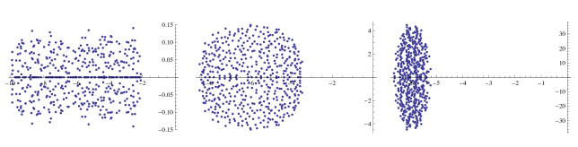
Figure 1. Eigenvalues of $M=D+gA$, $n=500$. The entries of $D$ are random numbers with uniform probability in $(-10,-2)$, while the independent entries of $A$ are random numbers with uniform probability in $(-4,4)$. $g=0.01,\,0.08,\,0.5$.

Fig.2 again depicts the eigenvalues of $M=D+g\,A$, with the same choice for the entries of $D$ and $A$, but with $g$ fixed to $1$ and increasing values of the order $n$. Only the vertical spread of the eigenvalues increases with $n$.

Figure 2. Eigenvalues of $M=D+gA$, $g=1$, $n=250,\,500,\,750$.

Clearly, the random matrices $M=D+g\,A$ satisfy the stability requirement that all eigenvalues have negative real part, independent of the size of the matrix and of the size of the entries of the antisymmetric component. However they would provide a model too rigid to describe a realistic community.

Remark 2.2.

Let’s consider again the matrix $M=D+g\,A$, where the entries of the diagonal matrix are negative, $a\leq d_{j}\leq b<0$ for all $j$, $A$ is any real antisymmetric matrix. The eigenvalues of $M$ are in the strip $a\leq{\rm Re}\,z_{j}\leq b$. If $O$ is an orthogonal matrix, consider the new matrix

$$M^{\prime}=O\,(D+g\,A)\,O^{-1}=\bar{D}+\tilde{S}+g\,A^{\prime}$$

where $\bar{D}$ is the diagonal part and $\tilde{S}$ is the off-diagonal part of the symmetric matrix $ODO^{-1}$. The entries of $\bar{D}$ are bounded:

$$a\leq{\bar{d}}_{j}=\sum_{k}O_{j,k}^{2}d_{k}\leq b$$

This suggests a possible structure for a real matrix $M$ with the desired spectral properties: the antisymmetric part $(M-M^{T})/2$ is arbitrary and the symmetric part $S=(M+M^{T})/2={\bar{D}}+\tilde{S}$ is diagonally dominant. A simple way to achieve it is to choose the diagonal elements $\bar{d}_{j}=S_{j,j}$ in the interval $(a,b)$ and the off-diagonal elements $S_{i,j}=O(1/\sqrt{n})$. This example is made explicit in Sect.4.

2.2. The Elliptic Ensemble

The best known elliptic ensemble is a model of random real matrices $J_{i,k}$ with Gaussian probabilities [20]:

(3) $$P(J)\,\prod_{i,j}dJ_{i,j}=\frac{1}{Z}\exp\left[-\frac{n}{2(1-\tau^{2})}{\rm Tr}(J\,J^{T}-\tau\,J\,J)\right]\,\prod_{i,j}dJ_{i,j},\quad|\tau|\leq 1$$

By writing $J=S+A$ with $S=\frac{1}{2}(J+J^{T})$ and $A=\frac{1}{2}(J-J^{T})$ one evaluates ${\rm Tr}(J\,J^{T})={\rm Tr}(S^{2}-A^{2})$ and ${\rm Tr}(J\,J)={\rm Tr}(S^{2}+A^{2})$. Then

$$P(S+A)=\frac{1}{Z}\left[\prod_{i=1}^{n}e^{-\frac{n}{2(1+\tau)}(S_{i,i})^{2}}\right]\left[\prod_{i=1}^{n}\prod_{k>i}e^{-\frac{n}{1+\tau}(S_{i,k})^{2}}\right]\left[\prod_{i=1}^{n}\prod_{k>i}e^{-\frac{n}{1-\tau}(A_{i,k})^{2}}\right]$$

$$Z=\left(\frac{\pi}{n}\right)^{n^{2}}\left[2(1+\tau)\right]^{n}\left[1-\tau^{2}\right]^{n(n-1)/2}$$

The set of $n^{2}$ random real variables is partitioned into three sets of independent central normal random variables: $n$ variables $S_{i,i}$ with $\sigma^{2}=(1+\tau)/n$, $\frac{n(n-1)}{2}$ variables $S_{i,k}$ ($i<k$) with $\sigma^{2}=(1+\tau)/(2n)$, and $\frac{n(n-1)}{2}$ variables $A_{i,k}$ ($i<k$) with $\sigma^{2}=(1-\tau)/(2n)$. One evaluates

$$\mathbb{E}\left[J_{i,k}\right]=0,\quad\mathbb{E}\left[J_{i,k}J_{k,i}\right]=\frac{\tau}{n},\quad\mathbb{E}\left[(J_{i,k})^{2}\right]=\frac{1}{n}.$$

In the limit $n\to\infty$, the distribution of the eigenvalues of $J_{n}\sqrt{n}$ converges to the uniform distribution on the elliptic region with semi-axes $a=(1+\tau)\sqrt{n}$, $b=(1-\tau)\sqrt{n}$.

Some decades of progress are evident in the more recent works [21, 22]. The following theorem is a generalization of the Circular Theorem, by Girko and Ginibre, and is important for the present discussion.

Theorem 2.3 (Elliptic theorem).

Let $M$ be a real random matrix such that:
a) pairs $\{M_{i,j}\,,\,M_{j,i}\}$, ${i\neq j}$, are i.i.d. random vectors and

$$\mathbb{E}(M_{1,2}\,M_{2,1})=\rho,\quad|\rho|\leq 1$$

b) $\mathbb{E}(M_{1,2})=\mathbb{E}(M_{2,1})=0$, $\mathbb{E}(M_{1,2}^{2})=\mathbb{E}(M_{2,1}^{2})=1$, $\mathbb{E}(M_{1,2}^{4}),\mathbb{E}(M_{2,1}^{4})\leq C$;
c) The diagonal entries $m_{i,i}$ are i.i.d. random variables with

$$\mathbb{E}(M_{1,1})=0\;,\quad\mathbb{E}(M_{1,1}^{2})<\infty$$

Then the distribution of the eigenvalues $x_{k}+iy_{k}$ of the matrix $\frac{1}{\sqrt{n}}M$ converges, in the limit $n\to\infty$, to the uniform distribution on the ellipse

$$\frac{x^{2}}{(1+\rho)^{2}}+\frac{y^{2}}{(1-\rho)^{2}}\leq 1$$

2.3. Dilute matrices

In realistic models the different species do not have all-to-all connectivity. We should expect most of the matrix elements of $M$ to vanish. As one introduces an increasing number of zero entries, the circular law continues to hold, up to a point.
Let us suppose that the $n^{2}$ real entries $M_{i,j}$ of the matrix $M$ are i.i.d. random variables with a probability $1-Q_{n}$ to be zero:

$$P\left(M_{i,j}\right)=Q_{n}\,\pi(M_{i,j})+(1-Q_{n})\,\delta(M_{i,j})$$

where $\pi(M_{i,j})$ is a probability distribution with variance $\sigma^{2}$.
If $0<Q_{n}<1-\frac{1}{n^{1-\alpha}}$, $0<\alpha\leq 1$, the eigenvalues of $M$ converge to the uniform distribution on a disk of radius $\sigma\,\sqrt{n\,Q_{n}}$ [23].
If $Q_{n}=p/n$, the graph associated to the matrix typically decomposes into a giant cluster ($p=1$ is a percolation transition) and a large number of small clusters, mostly trees. The spectral density of eigenvalues shows spikes corresponding to the eigenvalues of trees [24, 25, 26, 27, 28, 29].

Neri and Metz [30] obtained the analytic form of the spectrum of diluted random matrices with entries $\{M_{i,j},M_{j,i}\}$ that take values $(a,b)$, $(b,a)$ or $(0,0)$ according to a tuneable hierarchic structure of the graph of the matrix. In the dense limit it recovers the elliptic distribution.

S. Allesina and Si Tang [7] correctly argued that to consider elliptic ensembles (with the antisymmetric part greater than the symmetric part) with an amount of dilution increases the stability of the system. Still the axes of the ellipse are proportional to $\sqrt{n}$ and, for sufficiently large $n$ and if the center of the ellipse is kept fixed at a real negative value, the elliptic domain will not be confined to the left complex half-plane.

3. Antagonistic matrices

The goal of this investigation is to explore a class of real matrices useful to describe an ecological community, such that the real part of all the eigenvalues of the matrix is negative despite $n$ being large, in order to evade the stability-complexity paradox.

Definition 3.1.

An antagonistic matrix ${\mathcal{A}}$ is a real $n\times n$ matrix such that $\mathcal{A}_{i,i}=0$ and, for every pair $i<j$, the entries $\mathcal{A}_{i,j}$ and ${\mathcal{A}}_{j,i}$ have opposite sign or are both zero.

Remark 3.2.

If $\mathcal{A}$ is an antagonistic matrix, also $-\mathcal{A}$ and $\mathcal{A}^{T}$ are antagonistic. If $D$ is real diagonal then $D\mathcal{A}D^{-1}$ is antagonistic. If $P$ is a permutation matrix, also $P^{T}{\mathcal{A}}P$ is antagonistic, with same eigenvalues.

In ref.[31], it was shown by standard perturbation methods that the non-degenerate spectrum of a real symmetric matrix perturbed by an antisymmetric matrix is squeezed to a narrower rectangle in the complex plane. We show a similar result:

Proposition 3.3.

Let $D$ be a real diagonal matrix with entries $d_{1},\dots,d_{n}$, with non degenerate extremal values $d_{M}$ and $d_{m}$, and let ${\mathcal{A}}$ be an antagonistic matrix. For small $\epsilon$ and at leading order, the eigenvalues of $M(\epsilon)=D+\epsilon\,{\mathcal{A}}$ are in the strip

(4) $$d_{m}+\epsilon^{2}\frac{|\mathcal{A}^{2}_{m,m}|}{d_{M}-d_{m}}<z<d_{M}-\,\epsilon^{2}\frac{|\mathcal{A}^{2}_{M,M}|}{d_{M}-d_{m}}$$

Proof.

Let us expand in $\epsilon$ the characteristic polynomial:

$$P(z,\epsilon) =\det(z-D-\epsilon\mathcal{A})$$

$$=P(z,0)\exp[{\rm tr}\log(1-\epsilon(z-D)^{-1}\mathcal{A})]$$

(5) $$=P(z,0)\left[1-\frac{\epsilon^{2}}{2}\sum_{i,j}\frac{\mathcal{A}_{i,j}\mathcal{A}_{j,i}}{(z-d_{i})(z-d_{j})}+\mathcal{O}(\epsilon^{3})\right]$$

The term linear in $\epsilon$ is zero because $\mathcal{A}_{j,j}=0$. To leading order, the extremal eigenvalues of the perturbed matrix $M(\epsilon)$ are:

(6) $$\lambda_{\max}=d_{M}-\epsilon^{2}\sum_{j\neq M}\frac{|\mathcal{A}_{M,j}\mathcal{A}_{j,M}|}{d_{M}-d_{j}},\qquad\lambda_{\min}=d_{m}+\epsilon^{2}\sum_{j\neq m}\frac{|\mathcal{A}_{m,j}\mathcal{A}_{j,m}|}{d_{j}-d_{m}}$$

The result follows by a simple inequality. ∎

Proposition 3.4.

With the same setting of proposition 3.3, let the lowest eigenvalue $d_{\min}$ of $D$ have degeneracy $h$. Then a pair of eigenvalues of $M(\epsilon)$ are complex conjugate, and $h-2$ are unperturbed at order $\epsilon$.

Proof.

Let $\sigma$ be the set of $h$ indices such that $d_{j}=d_{min}$. The expansion (5) is

$$P(z,\epsilon)= P(z,0)\left[1-\frac{\epsilon^{2}}{2}\sum_{i,j\in\sigma}\frac{\mathcal{A}_{i,j}\mathcal{A}_{j,i}}{(z-d_{\min})^{2}}-\epsilon^{2}\sum_{i\in\sigma}\sum_{j\notin\sigma}\frac{\mathcal{A}_{i,j}\mathcal{A}_{j,i}}{(z-d_{\min})(z-d_{j})}+\dots\right]$$

The solution of $P(z,\epsilon)=0$ for $z=d_{\min}+\epsilon\delta_{1}+\epsilon^{2}\delta_{2}+\dots$ shows that $h-2$ minimal eigenvalues remain unchanged and two become complex:

$$\lambda=d_{\min}\pm i\frac{|\epsilon|}{\sqrt{2}}\sqrt{\sum_{i,j\in\sigma}|\mathcal{A}_{i,j}\mathcal{A}_{j,i}|}+\frac{\epsilon^{2}}{2}\sum_{i\in\sigma}\sum_{j\notin\sigma}\frac{\mathcal{A}_{i,j}\mathcal{A}_{j,i}}{d_{\min}-d_{j}}+\mathcal{O}(\epsilon^{3})$$

Note that $\delta_{2}>0$. A similar result would hold for a degenerate highest eigenvalue. ∎

3.1. Random antagonistic ensembles

The simplest model of an ensemble of random antagonistic matrices has a joint probability density for the $n^{2}-n$ matrix entries ${\mathcal{A}}_{i,j}$ in the form of a product of joint probability densities for the pairs, i.e. the pairs are independent random vectors, like in the elliptic ensemble:

(7) $$P\left({\mathcal{A}}\right)=\prod_{i<j}f_{i,j}({\mathcal{A}}_{i,j}\,,\,{\mathcal{A}}_{j,i})$$

where $f_{i,j}(x,y)=P(\mathcal{A}_{i,j}=x,\mathcal{A}_{j,i}=y)$. If $f_{i,j}(x,y)=f_{i,j}(y,x)$, the resulting marginal probabilities $p(\mathcal{A}_{i,j}=x)$ and $p(A_{j,i}=y)$ are equal.
The support of each pair density $f_{i,j}$ is a subset in $(x,y)$ plane where $x\,y\leq 0$. This constraint increases the stability of the model because it increases the weight of the antisymmetric component versus the symmetric component.
If $\pm\mathcal{A}$ belong to the ensemble with the same probability, it follows that if $z$ belongs to the spectrum of the ensemble, then the four points $\pm z$ and $\pm z^{*}$ belong to it with same probability.

Remark 3.5.

If the independent random pairs are chosen to be identically distributed and the random antagonistic model satisfies the conditions of theorem 2.3 then, in the large $n$ limit, the eigenvalues converge to a (slim) ellipse.
For the purpose of stability it is necessary to choose different probability distribution for the pairs.

The following proposition is reminiscent of the known property of a real antisymmetric matrix $A$: $\det A=0$ ($n$ odd), $\det A=(pf[A])^{2}=-pf[A]\cdot pf[A^{T}]$ ($n$ even).
We recall the notion of Pfaffian. Let $n$ be even. Given a triangular array $a=\{a_{i,j}\}$, $1\leq i<j\leq n$,

$$pf[a]=\sum_{P}{}^{\prime}\epsilon_{P}\,a_{i_{1},i_{2}}a_{i_{3},i_{4}}\dots a_{i_{n-1},i_{n}}$$

where the sum is on all permutations $P=\left(\begin{array}[]{cccc}1&2&\dots&n\\ i_{1}&i_{2}&\dots&i_{n}\end{array}\right)$ such that

$$i_{1}<i_{2},\,i_{3}<i_{4},\,\dots,i_{n-1}<i_{n},\quad\text{and}\quad i_{1}<i_{3}<i_{5}<\dots<i_{n-1}$$

$\epsilon_{P}$ is the sign of the permutation. If $n$ is odd, $pf[a]=0$ by definition.
In the case of a square matrix $M$, $pf[M]$ is a multinomial in the entries of the triangular array $\{M_{i,j}\}$, $1\leq i<j\leq n$. If $A$ is a real antisymmetric matrix, $pf[A]=-pf[A^{T}]$.

Proposition 3.6.

Let ${\mathcal{A}}$ belong to a random antagonistic ensemble where the joint probability density of the entries is the product of probability of independent pairs, as in eq.(5) and the average of each entry is zero, $\mathbb{E}\left[\mathcal{A}_{i,j}\right]=0$. Then:

$$\mathbb{E}\left[\det\mathcal{A}\right]=0 n$$ odd

$$\mathbb{E}\left[\det\mathcal{A}\right]=(-1)^{n/2}\mathbb{E}\left[\,pf[{\mathcal{A}}]\,\cdot\,pf[{\mathcal{A}}^{T}]\,\right]>0 n$$ even

The expectation of the characteristic polynomial $\mathbb{E}(\det[z\,I_{n}-\mathcal{A}])$ is a polynomial in $z^{2}$ with positive coefficients. In particular, $\mathbb{E}(\sum_{k}\lambda^{2}_{k})=\mathbb{E}({\rm tr}[\mathcal{A}^{2}])=-\sum_{i<j}\theta_{i,j}$ where $\theta_{i,j}=-\mathbb{E}(\mathcal{A}_{i,j}\mathcal{A}_{j,i})\geq 0.$

The proofs with the explicit expressions of the average Pfaffian or characteristic polynomial are given in the appendix, with two different techniques.

3.2. Simple probability measures and spectral domains

We briefly describe some simple probability densities for random antagonistic matrices, yielding the most common marginal probabilities. In the first three examples the independent pairs are identically distributed, $f_{i,j}(x,y)=f(x,y)$.

3.2.1. Gaussian marginal probability

$$f(x,y)=\frac{1}{\pi}e^{-\frac{1}{2}(x^{2}+y^{2})}\theta(-xy)$$

The marginal probabilities are standard normal

$$f(x)=\frac{1}{\pi}\int_{-\infty}^{\infty}dy\,e^{-(x^{2}+y^{2})/2}\theta(-xy)=\frac{1}{\sqrt{2\pi}}e^{-x^{2}/2}$$

and $\mathbb{E}[{\mathcal{A}}_{i,j}]=0$, $\mathbb{E}[({\mathcal{A}}_{i,j})^{2}]=1$, $\mathbb{E}[{\mathcal{A}}_{i,j}{\mathcal{A}}_{j,i}]=-\frac{2}{\pi}$.

3.2.2. Uniform marginal probability

$$f(x,y)=\begin{cases}1/2&\text{if $x\in(0,1)$ and $y\in(-1,0)$}\\ 1/2&\text{if $x\in(-1,0)$ and $y\in(-1,0)$}\\ 0&\text{otherwise}\end{cases}$$

The marginal probabilities are uniform in $(-1,1)$:

$$f(x)=\int_{-1}^{1}f(x,y)\,dy=\begin{cases}1/2&\text{if $x\in(-1,1)$}\\ 0&\text{otherwise}\end{cases}$$

Each random variable ${\mathcal{A}}_{i,k}$ is identically distributed, with $\mathbb{E}[\mathcal{A}_{i,j}]=0$, $\mathbb{E}[(\mathcal{A}_{i,j})^{2}]=\frac{1}{3}$, $\mathbb{E}[(\mathcal{A}_{i,j})^{4}]=\frac{1}{5}$ and, for every pair, $\mathbb{E}[{\mathcal{A}}_{i,k}{\mathcal{A}}_{k,i}]=-\frac{1}{4}$.

3.2.3. Marginal probability with support on two symmetric intervals

If the joint probability density for a pair has support on strips, the marginal probability has support on two disjoint intervals.
For example, let us define the function

$$g_{w}(x)=\begin{cases}\frac{1}{2w}&\text{if $-w<x<w$}\\ 0&\text{ otherwise}\end{cases}\quad 0<w<1$$

and the joint probability density of the pair

$$f(x,y)=\tfrac{1}{2}\left[g_{w}(x+1)\,g_{w}(y-1)+g_{w}(x-1)g_{w}(y+1)\right]$$

and $\mathbb{E}\left[{\mathcal{A}}_{i,k}{\mathcal{A}}_{k,i}\right]=-1$. The marginal densities are $f(x)=\tfrac{1}{2}\left[g_{w}(x-1)+g_{w}(x+1)\right]$, that is, the probability density of any ${\mathcal{A}}_{i,k}$ has support on the union of two intervals, $(-1-w,-1+w)\,\cup\,(1-w,1+w)$, with $\mathbb{E}[\mathcal{A}_{i,j}]=0$, $\mathbb{E}[(\mathcal{A}_{i,j})^{2}]=1+\frac{w^{2}}{3}$.

Remark 3.7.

The three models agree with the conditions in Proposition 2.3. The parameter $\rho$ describing the elliptic domain of the spectrum in the limit $n\to\infty$ of the random antagonistic matrix is

$$\rho=\begin{cases}-\frac{2}{\pi}&\text{\rm Gaussian}\\ -\frac{3}{4}&\text{\rm uniform}\\ -\frac{3}{3+w^{2}}&\text{\rm two intervals}\end{cases}$$

3.3. Independent pairs not-identically distributed.

A useful probability density for the antagonistic matrix is

$$f_{i,k}(x,y)=\begin{cases}C_{i,k}&\text{if $x\in(1,1+\delta)$ and $y\in(-1-\delta,-1)$}\\ C_{i,k}&\text{if $y\in(1,1+\delta)$ and $x\in(-1-\delta,-1)$ }\\ 0&\text{otherwise}\end{cases},\quad\delta=\frac{c}{1+(k-i)^{p}}$$

As the order $n$ of the antagonistic matrix ${\mathcal{A}}$ increases, the pair of entries far from the diagonal are increasingly similar to an antisymmetric matrix, see fig.3. All eigenvalues are in a strip $-a<Re\,z<a$ where the width of the strip does not increase with $n$; actually it slightly decreases.

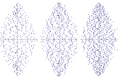
Figure 3. Eigenvalues of a random antagonistic matrix with $c=50$, $p=8$, $n=400,\,600,\,800.$

Next, we add a diagonal matrix, with random entries $d_{j}$ uniform in $(-6,-4)$. The eigenvalues of $D+{\mathcal{A}}$ are shown in fig.4. They are like the plots in fig.3, but shifted by 5 units to the left in the complex plane.

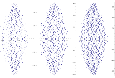
Figure 4. The eigenvalues of $D+\mathcal{A}$, $n=400,\,600,\,800$.

4. “Small” symmetric plus “big” antisymmetric.

A simple way to define an ensemble of real random matrices with eigenvalues that with high probability are in the le ft complex half-plane, is to consider real matrices

$$D+\frac{1}{\sqrt{n}}S+A$$

where the symmetric matrix $S$ has zero diagonal and is “small” compared to the antisymmetric matrix $A$, and $D$ is a properly chosen diagonal matrix.

If the entries $S_{i,j}$, for $i>j$, are i.i.d. with zero mean and variance $\sigma_{S}^{2}$ , most of the eigenvalues of the matrix $S/\sqrt{n}$ are, for large $n$, in the interval $(-2\sigma_{S}\,,\,2\sigma_{S})$.
If the entries $A_{i,j}$, for $i>j$, are i.i.d. with zero mean and variance $\sigma_{A}^{2}$, most of its eigenvalues, for large $n$, are in the interval $(-2i\sigma_{A}\sqrt{n}\,,\,2i\sigma_{A}\sqrt{n})$.
Therefore, for large $n$, the eigenvalues of the matrix $\frac{1}{\sqrt{n}}S+A$ are with high probability inside the rectangular box with fixed horizontal side $-2\sigma_{S}\,<x<\,2\sigma_{S}$ and increasing vertical side $-2i\sigma_{A}\sqrt{n}\,<y<\,2i\sigma_{A}\sqrt{n}$.
Fig.5 shows $800$ eigenvalues of a matrix $S/\sqrt{n}+A$ with entries $S_{i,j}$ ($i>j$) uniformly distributed in $(-30,30)$ (then $\sigma_{s}=30/\sqrt{3}$), and $A_{i,j}$ ($i>j$) uniformly distributed in $(-10,10)$ (then $\sigma_{A}=10/\sqrt{3}$).

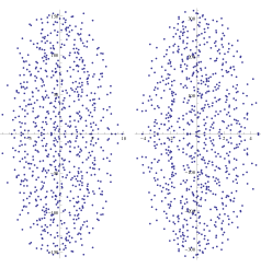
Figure 5. Left: combined eigenvalues of $4$ random matrices $n=200$. Right: eigenvalues of a single random matrix $n=800$.

Already for $n=200$ the eigenvalues appear to be confined in a rectangular domain with sides $20\times 160$, much smaller then the estimated rectangular domain with sides $\left(\frac{120}{\sqrt{3}}\sim 69.2\right)\,\times\left(\frac{40\sqrt{200}}{\sqrt{3}}\sim 326.6\right)$.
Furthermore the right panel in fig.5 shows that the horizontal side of the domain decreases for increasing values of $n$. This shrinking effect is analogous to that shown in Section 2.1 for the matrix $D+g\,A$.
One may also remark that with the above distribution for $S_{i,j}$ and $A_{i,j}$ the random matrix $\frac{1}{\sqrt{n}}S+A$ is not antagonistic, but it is antagonistic if the distribution of the $A_{i,j}$ is chosen to have a gap, for instance uniform distribution on $(-10,-1.5)\cup(1.5,10)$ , then $\max|S_{i,j}|/\sqrt{n}<1.5$ for $n\geq 800$ .

Finally we add a diagonal matrix: $D+\frac{1}{\sqrt{n}}S+A$ . With proper choice of $D$, the domain is shifted so that all eigenvalues are, with high probability in the left part of the complex plane. Fig.6 shows the eigenvalues for $n=800$, with $\frac{1}{\sqrt{n}}S+A$ having the above distribution and the diagonal entries $d_{j}$ being uniformly distributed in $(-10,-5)$. All the eigenvalues of the simulation have the real part in the interval $-12.58<x<-3.246$. It is reasonable to expect that for greater values of $n$ the eigenvalues would be confined into a more narrow strip centered around $x\sim-7.5$.

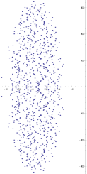
Figure 6.

5. Appendix

Proof 1 (combinatorial). $\mathbb{E}\left[\det{\mathcal{A}}\right]=\sum_{P}\epsilon_{P}\mathbb{E}\left[\,\mathcal{A}_{1,i_{1}}\dots\mathcal{A}_{n,i_{n}}\right]$. In analogy with Wick’s theorem, the expectation of each term of the sum factorizes and is non-zero only if $n$ is even, and if for every factor $\mathcal{A}_{k,n_{k}}$ there is the symmetric factor $\mathcal{A}_{n_{k},k}$. For example, for $n=4$ the non-zero terms are:

$$\mathbb{E}\left[\det\mathcal{A}\right]=\mathbb{E}\left[\mathcal{A}_{1,2}\mathcal{A}_{2,1}\mathcal{A}_{3,4}\mathcal{A}_{4,3}+\mathcal{A}_{1,3}\mathcal{A}_{2,4}\mathcal{A}_{3,1}\mathcal{A}_{4,2}+\mathcal{A}_{1,4}\mathcal{A}_{2,3}\mathcal{A}_{3,2}\mathcal{A}_{4,1}\right]>0.$$

The expectation is non-vanishing only for the permutations which are products of $n/2$ cycles of length two. The number $c_{n}$ of terms that contribute to the expectation value of $\det[{\mathcal{A}}]$ is

$$c_{n}=(n-1)(n-3)\dots 3\cdot 1=\frac{(n)!}{2^{n/2}\left(\frac{n}{2}\right)!}$$

The sign of such permutations is $\epsilon_{P}=(-1)^{3n/2}$ .
For an antagonistic matrix, the Pfaffian is multilinear in the entries of the upper triangular part of the matrix, $\mathcal{A}_{i,j}$ with $i<j$. For example ($n=4$):

$$pf\left[{\mathcal{A}}\right]=\mathcal{A}_{1,2}\mathcal{A}_{3,4}-\mathcal{A}_{1,3}\mathcal{A}_{2,4}+\mathcal{A}_{1,4}\mathcal{A}_{2,3},\quad pf\left[{\mathcal{A}}^{T}\right]=\mathcal{A}_{2,1}\mathcal{A}_{4,3}-\mathcal{A}_{3,1}\mathcal{A}_{4,2}+\mathcal{A}_{4,1}\mathcal{A}_{3,2}$$

If $n$ is even, the number of terms in $pf\left[\mathcal{A}\right]$ is $c_{n}$.

In the evaluation of the average $\mathbb{E}\left[\,pf[\mathcal{A}]\,\cdot\,pf[\mathcal{A}^{T}]\,\right]$ the only non-zero terms are the $c_{n}$ terms that are product of entries symmetric with respect of the matrix diagonal. $\Box$

Proof 2 (Grassmann integral). We compute the ensemble average of the characteristic polynomial $p(z)=\mathbb{E}[\det\left(z\,I_{n}-{\mathcal{A}}\right)]$, via a representation of the determinant of a matrix as a Gaussian integral on anti commuting variables ${\bar{\psi}}_{i}$ , $\psi_{i}$ , $i=1,\dots,n$.

$$\det\left(z\,I_{n}-{\mathcal{A}}\right)= \int\prod_{k=1}^{n}\left(d{\bar{\psi}}_{k}d\psi_{k}\right)\,e^{\sum_{i,j}{\bar{\psi}}_{i}\left(z\,I-{\mathcal{A}}\right)_{i,j}\psi_{j}}=$$

$$= \int\prod_{k=1}^{n}\left(d{\bar{\psi}}_{k}d\psi_{k}\right)\,e^{z\sum_{r=1}^{n}{\bar{\psi}}_{r}\psi_{r}}\,e^{-\sum_{i<j}{\bar{\psi}}_{i}{\mathcal{A}}_{i,j}\psi_{j}+{\bar{\psi}}_{j}{\mathcal{A}}_{j,i}\psi_{i}}=$$

$$= \int\prod_{k=1}^{n}\left(d{\bar{\psi}}_{k}d\psi_{k}\right)\,\prod_{r=1}^{n}\left(1+z\,{\bar{\psi}}_{r}\psi_{r}\right)\times$$

$$\times\prod_{i<j}\left(1-{\bar{\psi}}_{i}{\mathcal{A}}_{i,j}\psi_{j}-{\bar{\psi}}_{j}{\mathcal{A}}_{j,i}\psi_{i}-{\bar{\psi}}_{i}\psi_{i}{\bar{\psi}_{j}}\psi_{j}\,{\mathcal{A}}_{i,j}{\mathcal{A}}_{j,i}\right)$$

The ensemble average is taken, with $\theta_{i,j}=-\mathbb{E}[{\mathcal{A}}_{i,j}{\mathcal{A}}_{j,i}]\geq 0$:

$$p(z)= \int\prod_{k=1}^{n}\left(d{\bar{\psi}}_{k}d\psi_{k}\right)\,\prod_{r=1}^{n}\left(1+z\,{\bar{\psi}}_{r}\psi_{r}\right)\,\prod_{i<j}\left(1+{\bar{\psi}}_{i}\psi_{i}{\bar{\psi}_{j}}\psi_{j}\,\theta_{i,j}\right)=$$

$$= z^{n}+z^{n-2}\sum_{i<j}\theta_{i,j}+z^{n-4}\sum^{\prime}_{i_{1}<j_{1}\,,\,i_{2}<j_{2}}\theta_{i_{1},j_{1}}\theta_{i_{2},j_{2}}+$$

$$+z^{n-6}\sum^{\prime}_{i_{1}<j_{1}\,,i_{2}<j_{2}\,,\,i_{3}<j_{3}}\theta_{i_{1},j_{1}}\theta_{i_{2},j_{2}}\theta_{i_{3},j_{3}}+\ldots;$$

if $n$ is even, the sum terminates with

(8) $$\mathbb{E}[\det\mathcal{A}]=\sum^{\prime}_{i_{k}<j_{k}}\theta_{i_{1},j_{1}}\dots\theta_{i_{n/2},j_{n/2}}.$$

The primed sums are restricted to have all indices different and $i_{1}<i_{2}<\dots<i_{k}$. $\Box$

References

- [1] T. Seligman, J. Verbaarschot and M. Zirnbauer, J. Phys. A: Math. Gen. 18 (1985) 2751.
- [2] G. Casati, L. Molinari, and F. Izrailev, Scaling properties of band random matrices, Phys. Rev. Lett. 64 (1990), 1851–1854. G. Casati, F. Izrailev and L. Molinari, J. Phys. A: Math. Gen. 24 (1991) 4755.
- [3] G. Casati, B. V. Chirikov, I. Guarneri, F. M. Izrailev, Band-random-matrix model for quantum localization in conservative systems, Phys. Rev. E 48 (1993), R1613.
- [4] T. Spencer, Random Band Matrices and Random Sparse Matrices, chapter in Handbook on Random Matrix Theory, Editors: G. Akemann, J. Baik, and Ph. Di Francesco. Oxford University Press, 2011.
- [5] K. Rajan and L. F. Abbott, Eigenvalue Spectra of Random Matrices for Neural Networks, Phys. Rev. Lett. 97, 188104 (2006).
- [6] A. Amir, N. Hatano and D. R. Nelson, Localization in non-Hermitian chains with excitatory/inhibitory connections, arXiv:1512.05478.
- [7] S. Allesina and Si Tang, The stability – complexity relationship at age 40: a random matrix perspective, Popul. Ecol. 57 (2015), 63–75.
- [8] R. M. May, Will a large complex system be stable?, Nature 238, 413–414 (1972).
- [9] C. Bordenave and D. Chafai, Around the circular law, Probability Surveys Vol. 9 (2012) 1–89.
- [10] R. A. Horn and C. R. Johnson, Matrix Analysis, chapter 5 and 6, Cambridge Univ. Press 1985.
- [11] ESA Report, D. U. Hooper et al., Effects of biodiversity on ecosystem functioning: a consensus of current knowledge, Ecological Monographs, 75(1), 2005, 3–35, by the Ecological Society of America.
- [12] A. Roberts, Stability of a feasible random system , Nature 251 (1974) 607–608.
- [13] P. Kirk, D. M. Y. Rolando, A. L. MacLean and M. P. H. Stumpf , Conditional random matrix ensembles and the stability of dynamical systems, New J. Phys. 17 (2015) 083025.
- [14] D. T. Haydon, Maximally stable model ecosystem can be highly connected, Ecology 81 (9), (2000) 2631–2636.
- [15] K. S. McCann, The diversity - stability debate, Nature 405 (2000), 228–233.
- [16] M. A. Fortuna, D. B. Stouffer, J. M. Olesen, P. Jordano, D. Mouillot, B. R. Krasnov, R. Poulin and J. Bascompte, Nestedness versus modularity in ecological networks: two sides of the same coin?, J. of Animal Ecology 79 (2010), 811–817.
- [17] D. Hershkowitz, Recent directions in matrix stability, Linear Algebra Appl. 171 (1992) 161-186.
- [18] Y. V. Fyodorov and B. A. Khoruzhenko, A nonlinear analogue of May-Wigner instability transition, arXiv:1509.05737 [cond-mat.dis-nn] (sept.2015).
- [19] M. L. Mehta, Matrix Theory, Selected Topics and Useful Results, chapt. 11, Les Editions de Physique 1989.
- [20] H. J. Sommers, A. Crisanti, H. Sompolinsky and Y. Stein, Spectrum of large random asymmetric matrices, Phys. Rev. Lett. 60 (1988), 1895.
- [21] A. Naumov, Elliptic law for real random matrices, arXiv:1201.1639.
- [22] Hoi H. Nguyen and S. O’Rourke, The elliptic law, Int. Math. Res. Notices (2015) Vol. 2015, 7620–7689.
- [23] P. Matchett Wood, Universality and the circular law for sparse random matrices, Ann. Appl. Probab. 22, No.3 (2012), 1266–1300.
- [24] G. J. Rodgers and A. J. Bray, Density of states of a sparse random matrix , Phys. Rev. B 37 (1988), 3557. G. J. Rodgers and C. De Dominicis, Density of states of sparse random matrices, J. of Phys. A: Math. Gen 23 (1990), 1567.
- [25] Y.V. Fyodorov and A.D. Mirlin, On the density of states of sparse random matrices, J. of Phys. A: Math. Gen. 24 (1991), 2219.
- [26] M. Bauer and O. Golinelli, Random incidence matrices: moments of the spectral density, J. Stat. Phys. 103 (2001), 301.
- [27] G. Semerjian and L. F. Cugliandolo, Sparse random matrices: the eigenvalue spectrum revisited, J. of Phys. A: Math. Gen. 35 (2002), 4837.
- [28] R. Kühn, Spectra of sparse random matrices, J. Phys. A: Math. Theor. 41 (2008) 295002 (21pp).
- [29] T. Rogers, New Results on the Spectral Density of Random Matrices, Ph.D. thesis, Dept. of Math., King’ s College London, July 2010
- [30] I. Neri and F. L. Metz, Spectra of sparse non-Hermitian random matrices: an analytical solution, Phys. Rev. Lett 109 (2012) 030602 (5pp).
- [31] J. Bloch, F. Bruckmann, N. Meyer and S. Schierenberg, Level spacings for weakly asymmetric real random matrices and application to two-color QCD with chemical potential, JHEP 08 (2012) 066.