Minimising the number of triangular edges

Abstract

We consider the problem of minimising the number of edges that are contained in triangles, among $n$-vertex graphs with a given number of edges. We prove a conjecture of Füredi and Maleki that gives an exact formula for this minimum, for sufficiently large $n$.

1 Introduction

Mantel [8] proved that a triangle-free graph on $n$ vertices has at most $\lfloor n^{2}/4\rfloor$ edges. In other words, a graph on $n$ vertices with at least $\lfloor n^{2}/4\rfloor+1$ edges contains a triangle. A natural question arises from this classical result: how many triangles must such a graph have? And, indeed, Rademacher [10] extended Mantel’s result by showing that any graph on $n$ vertices with $\lfloor n^{2}/4\rfloor+1$ edges contains at least $\lfloor n/2\rfloor$ triangles, a bound that can readily be seen to be best possible (see Figure 1).

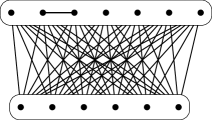
Figure 1: $\lfloor n^{2}/4\rfloor+1$ edges, $\lfloor n/2\rfloor$ triangles, $2\lfloor n/2\rfloor+1$ triangular edges

Erdős [1] conjectured that a further generalisation holds: any graph on $n$ vertices with at least $\lfloor n^{2}/4\rfloor+l$ edges contains at least $l\lfloor n/2\rfloor$ triangles, for every $1\leq l<\lfloor n/2\rfloor$. Erdős [1, 2] proved his conjecture for $l\leq cn$ for some constant $c>0$. It is not hard to see that the bound on the number of triangles is best possible, by adding $l$ edges, that do not span a triangle, to the larger part of the complete bipartite graph $K_{\lfloor n/2\rfloor,\lceil n/2\rceil}$. Furthermore, it is not hard to see that the bound on $l$ is best possible, by considering a similar construction.

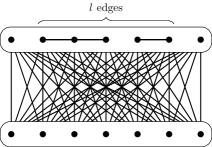
Figure 2: $\lfloor n^{2}/4\rfloor+l$ edges, $l\lfloor n/2\rfloor$ triangles

Erdős’s conjecture was resolved by Lovász and Simonovits [6], who also characterised [7] the graphs with $n$ vertices and $\lfloor n^{2}/4\rfloor+l$ edges that minimise the number of triangles, for every $l\leq cn^{2}$ where $c>0$ is fixed. Razborov [11] determined the asymptotic behaviour of the number of triangles in graphs with $n$ vertices and $\lfloor n^{2}/4\rfloor+l$ edges where $l=\Omega(n^{2})$.

In this paper we consider a similar problem, concerning the number of edges that are contained in triangles (we shall call such edges triangular edges) rather than the number of triangles. The first result in this direction was obtained by Erdős, Faudree and Rousseau [3] who proved that any graph with $n$ vertices and $\lfloor n^{2}/4\rfloor+1$ edges has at least $2\lfloor n/2\rfloor+1$ triangular edges. This bound is best possible (see Figure 1).

It is very natural, similarly to the question about the number of triangles, to ask how many triangular edges an $n$-vertex graph with $e$ edges must have, where $e$ is any integer satisfying $\lfloor n^{2}/4\rfloor<e\leq\binom{n}{2}$. After some thought, a natural example comes to mind. Given integers $a,b,c$, we denote by $G(a,b,c)$ the graph with $n=a+b+c$ vertices, which consists of a clique $A$ of size $a$ and two independent sets $B$ and $C$ of sizes $b$ and $c$ respectively, such that all edges between $B$ and $A\cup C$ are present, and there are no edges between $A$ and $C$ (see Figure 3).

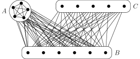
Figure 3: The graph $G(a,b,c)$ (here $a=4,b=6,c=5$)

Note that the graph $G(a,b,c)$ has $\binom{a}{2}+b(a+c)$ edges, $bc$ of them are non-triangular. We remark that the extremal example (depicted in Figure 1) for the aforementioned result by Erdős, Faudree and Rousseau [3] is isomorphic to $G(2,\lfloor n/2\rfloor,\lceil n/2\rceil-2)$.

Füredi and Maleki [4] conjectured that the minimisers of the number of triangular edges are graphs of the form $G(a,b,c)$, or subgraphs of such graphs.

Conjecture 1.

Let $n$ and $e>\lfloor n^{2}/4\rfloor$ be integers and let $G$ be a graph with $n$ vertices and $e$ edges that minimises the number of triangular edges. Then $G$ is a subgraph of a graph $G(a,b,c)$ for some $a,b,c$.

The condition that $G$ is a subgraph of a graph $G(a,b,c)$ (rather than simply requiring equality) is due to the fact that we specify the exact number of edges, so the minimiser may be isomorphic to $G(a,b,c)$ with a few edges removed.

Conjecture 1 is a generalisation of the case of $n$-vertex graphs with $\lfloor n^{2}/4\rfloor+1$ edges, where, as mentioned above, the minimiser is indeed $G(2,\lfloor n/2\rfloor,\lceil n/2\rceil-2)$.

The conjecture implies, in particular, that every graph with $n$ vertices and $e$ edges has at least the following number of triangular edges:

$$g(n,e)=\min\{e-bc:a+b+c=n,\binom{a}{2}+b(a+c)\geq e\}.$$

Füredi and Maleki [4] proved an approximate version of the latter statement, which reads as follows.

Theorem 2 (Füredi and Maleki [4]).

Every $n$-vertex graph with $e$ edges has at least $g(n,e)-3n/2$ triangular edges.

Our main result is an exact version of Theorem 2: we shall prove that a graph with $n$ vertices and $e$ edges has at least $g(n,e)$ triangular edges, provided that $n$ is large enough.

Before we state our result, we make a few remarks. We find it convenient to consider a reformulation of the latter statement. Firstly, it turns out to be more convenient to consider the clearly equivalent problem of maximising the number of non-triangular edges among $n$-vertex graphs with $e$ edges. Thus, given a graph $G$, we denote by $t(G)$ the number of non-triangular edges in $G$. Secondly, given $n$ and $e$, instead of restricting our attention to $n$-vertex graphs with exactly $e$ edges, we consider $n$-vertex graphs with at least $e$ edges. Since the maximum number of non-triangular edges cannot increase by adding edges (assuming that we have at least $\lfloor n^{2}/4\rfloor$ edges), this does not affect the problem of maximising the number of non-triangular edges, yet it allows us to concentrate on graphs $G(a,b,c)$ without having to consider their subgraphs.

We are now ready to state our main result.

Theorem 3.

There exists $n_{0}$ such that for any graph $G$ with at least $n_{0}$ vertices there is a graph $H=G(a,b,c)$ (for some integers $a,b,c$) that satisfies $|H|=|G|$, $e(H)\geq e(G)$ and $t(H)\geq t(G)$.

We note that Theorem 3 comes close to proving Conjecture 1 (for sufficiently large $n$) as it shows that the minimum number of triangular edges is attained by a graph $G(a,b,c)$ or a subgraph of $G(a,b,c)$, but we do not explicitly show that such graphs are the only minimisers.

1.1 Structure of the paper

The proof of our main result, Theorem 3, is divided into three parts, according to the number of edges: graphs that are close to being bipartite, i.e., where the number of edges is close to $n^{2}/4$; graphs that are close to being complete, i.e., the number of edges is close to $\binom{n}{2}$; and the middle range, where the number of edges is bounded away from both $n^{2}/4$ and $\binom{n}{2}$.

We state Theorems 4, 5 and 6, which are the theorems corresponding to the aforementioned three ranges, in Section 2, and give an overview of their proofs. In Section 3 we describe the tools that we shall use and introduce relevant notation. We prove the three theorems in Sections 4, 5 and 6: Theorem 4, which deals with graphs with close to $n^{2}/4$ edges, will be proved in Section 4; the proof of Theorem 5, for the middle range, is the heart of this paper and will be given in Section 5; and Theorem 6 will be proved in Section 6. We conclude the paper with Section 7 where we make some remarks and mention open problems.

2 Overview

We split the proof of Theorem 3 into three part, according to the number of edges $e$. We state the theorems corresponding to these three parts here.

The following theorem deals with $e$ that is close to $n^{2}/4$, i.e. $e\leq(1/4+\delta)n^{2}$, where $\delta$ is a sufficiently small constant.

Theorem 4.

There exist $n_{0}$ and $\delta>0$ such that the following holds. Let $G$ be a graph with $n\geq n_{0}$ vertices and $e$ edges, where $n^{2}/4\leq e\leq(1/4+\delta)n^{2}$. Then there is a graph $H=G(a,b,c)$ that satisfies $|H|=n$, $e(H)\geq e$ and $t(H)\geq t(G)$.

The next theorem considers the case where $e$ is bounded away from $n^{2}/4$ and $\binom{n}{2}$, namely $(1/4+\delta)n^{2}\leq e\leq(1/2-\delta)n^{2}$ for any constant $\delta>0$.

Theorem 5.

For every $\delta>0$ there exist $n_{0}$ such that the following holds. Let $G$ be a graph with $n\geq n_{0}$ vertices and $e$ edges, where $(1/4+\delta)n^{2}\leq e\leq(1/2-\delta)n^{2}$. Then there is a graph $H=G(a,b,c)$ that satisfies $|H|=n$, $e(H)\geq e$ and $t(H)\geq t(G)$.

Finally, we consider the remaining case, when $e$ is close to $\binom{n}{2}$, i.e. $e\geq(1/2-\delta)n^{2}$ for $\delta$ sufficiently small.

Theorem 6.

There exist $n_{0}$ and $\delta>0$ such that the following holds. Let $G$ be a graph with $n\geq n_{0}$ vertices and $e$ edges, where $e\geq(1/2-\delta)n^{2}$. Then there is a graph $H=G(a,b,c)$ that satisfies $|H|=n$, $e(H)\geq e$ and $t(H)\geq t(G)$.

We now try to give some insight into our proofs. The rough plan in the proof of each of the theorem is the same. Assuming that $G$ is a graph on $n$ vertices and at least $e$ edges, that maximises the number of non-triangular edges, we first try to obtain information about the rough structure of the graph. In each of the cases, we find a partition of the vertices $\{A,B,C\}$, where the three parts relate to the three parts in a graph $G(a,b,c)$, in a way that will be explained in the proofs. In the next stage we use lower bounds on the number of non-triangular edges (coming from examples $G(a,b,c)$) to estimate the size of the sets $A,B,C$. The final stage uses the estimates on the sizes to conclude that $G$ has the required structure, namely, it is isomorphic to the graph $G(|A|,|B|,|C|)$.

The proofs of the two extremal cases, where $e$ is close to either $n^{2}/4$ or $\binom{n}{2}$, are considerably easier than the middle range. The main reason for that is that in the extremal cases, it is fairly easy to show that the graph $G$ should be close to a graph $G(a,b,c)$, whereas in the middle range, getting any handle on the structure of the graph is hard, and the initial structural properties that we find are less restrictive than in the two extremal cases.

To help us with the proof of the middle range, we introduce two tools. The first one is a process of ‘compression’ that allows us to ‘simplify’ a graph without decreasing the number of edges or non-triangular edges. The second is the ‘exchange lemma’, that allows us to ‘exchange’ edges by non-triangular edges (and vice versa), i.e. by moderately reducing the number of edges, we can increase the number of non-triangular edges by a given amount. Both these tools will be presented and explained in Section 3.

3 Tools

In this section we introduces the tools that will be used in the paper. We start by describing some notation and simple definitions in Subsection 3.1. We introduce the notion of weighted graphs in Subsection 3.2 and list some results by Füredi and Maleki [4] that involve weighted graphs. An important tool in the proof of the middle range is the so-called Exchange Lemma, Lemma 13. We prove Lemma 13 and explain its importance in Subsection 3.3. Our last tool is the notion of compressed graphs which is a class of graphs with somewhat restrictive structure. In Subsection 3.4, we give our definition of a compressed graph in and prove Lemma 16, that shows that it suffices to prove Theorem 3 for compressed graphs.

3.1 Notation

The following notation is standard. Write $|G|$ for the order of a graph $G$ and $e(G)$ for the number of edges in $G$. We denote the degree of $u$ in $G$ by $\deg_{G}(u)$, or $\deg(u)$ if $G$ is clear from the context. Given a set $U$ of vertices of $G$, we denote by $G[U]$ the graph induced by $G$ on $U$.

We now turn to notation that is more specific to our context. An edge $e\in E(G)$ is called triangular if it is contained in a triangle of $G$. Similarly, we say that $e$ is non-triangular if it is not contained in a triangle. We denote by $t(G)$ the number of non-triangular edges of $G$.

Given a vertex $u$, a vertex $v$ is a triangular neighbour of $u$, if $uv$ is a triangular edge. Similarly, the triangular neighbourhood of $u$ is the set of triangular neighbours of $u$, and the triangular degree of $u$ is the number of triangular edges adjacent to $u$. The notions of a non-triangular neighbour, non-triangular neighbourhood and non-triangular degree can defined similarly. We denote the non-triangular degree of $u$ in $G$ by $\deg_{\text{Non-}\Delta}(u)$. A vertex $u$ is called triangular if $\deg_{\text{Non-}\Delta}(u)=0$, i.e., if all edges adjacent to $u$ are triangular.

We say that a set of vertices $U\subseteq V(G)$ is a set of clones if any two vertices in $U$ have the same neighbourhood in $G$. In particular, a set of clones is independent. For example, in $G(a,b,c)$ the sets $B$ and $C$ are sets of clones. We remark that the notion of clones will play an important role in the definition of a compressed graph (which will be defined in Subsection 3.4).

We now introduce the natural notion of an optimal graph.

Definition 7.

A graph $G$ on $n$ vertices is called optimal if there is no graph $H$ on $n$ vertices such that either $t(H)>t(G)$ and $e(H)\geq e(G)$ or $e(H)>e(G)$ and $t(H)\geq t(G)$.

In other words, $G$ is optimal if it maximises $t(G)$ among graphs with $n$ vertices and at least $e(G)$ edges and, in addition, it maximises $e(G)$ among graphs with $n$ vertices and at least $t(G)$ non-triangular edges.

It clearly suffices to prove the main result, Theorem 3, for optimal graphs. The following observation is a simple property of optimal graphs.

Observation 8.

Let $G$ be an optimal graph and let $u$ and $v$ be vertices in $G$. Then either $\deg(u)\geq\deg(v)-1$ or $\deg_{\text{Non-}\Delta}(u)\geq\deg_{\text{Non-}\Delta}(v)-1$.

• Suppose that $\deg(u)\leq\deg(v)-2$ and $\deg_{\text{Non-}\Delta}(u)\leq\deg_{\text{Non-}\Delta}(v)-2$. Consider the graph $G^{\prime}$ obtained by removing the edges adjacent to $u$ and adding the edges between $u$ and the neighbours of $v$. Then $e(G^{\prime})\geq e(G)-\deg(u)+\deg(v)-1>e(G)$ and, similarly, $t(G^{\prime})>t(G)$, contradicting the assumption that $G$ is optimal. ∎

We shall use big-O notation extensively throughout this paper, so, for the sake of clarity, we briefly explain how we interpret the symbols $O$, $o$ and $\Omega$. We write $f(n)=O(g(n))$ if there exists an absolute constant $C>0$ such that $|f(n)|\leq C|g(n)|$. In particular, the expression $f(n)=g(n)+O(h(n))$ consists of the following inequalities: $g(n)-C|h(n)|\leq f(n)\leq g(n)+C|h(n)|$. Similarly, $f(n)=o(g(n))$ means that $\lim_{n\rightarrow\infty}|f(n)/g(n)|=0$. Finally, we write $f(n)=\Omega(g(n))$ if $f(n)\geq C\cdot g(n)$ for an absolute constant $C>0$.

Throughout this paper, we omit integer parts whenever they do not affect the argument. We always assume that $n$ is large.

3.2 Weighted graphs

Our most basic tool is the concept of a weighted graph, which is a graph whose vertices have non-negative weights. The total weight of a weighted graph $G$ is the sum of the weights of its vertices and is denoted by $|G|$. Throughout this paper we require that the number of vertices of a weighted graph does not exceed its total weight. Equivalently, we require that the average weight of a vertex in a weighted graph is at least $1$.

Given weighted graphs $G$ and $H$ we say that $H$ is a weighted subgraph of $G$ if, as graphs, $H$ is a subgraph of $G$. Note that this definition does not impose any conditions on the weight function of $H$. In particular, if $H$ is a weighted subgraph of $G$ then the weight in $H$ of a vertex in $H$ may be larger than its weight in $G$.

Given a weighted graph $G$ with weight function $w:V(G)\to\mathbb{R}^{\geq 0}$ we define $e(G)$ to be the sum of $w(u)w(v)$ over all edges $uv$ of $G$. Similarly, we define $t(G)$ to be the same sum over the non-triangular edges of $G$. Note that any graph $G$ can be seen either as a graph or as a weighted graph whose every vertex has weight $1$, and the definitions of $|G|,e(G)$ and $t(G)$ do not depend on the point of view.

The notions of the degree and the non-triangular degree of a vertex may be similarly generalised to weighted graphs. For instance, the degree of $u$ in a weighted graph $G$ is the sum of weights of the neighbours of $u$. We use the notation $\deg(u)$ and $\deg_{\text{Non-}\Delta}(u)$ for the degree and the non-triangular degree of a vertex $u$ in a weighted graph.

We now define a good weighted graph (see also Figure 4).

Definition 9.

We call a weighted graph $G$ good if its vertex set can be partitioned into a set $K$ that induces a clique, and a pair $(u,v)$ of adjacent vertices, such that $uv$ is the only non-triangular edge in $G$.

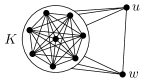
Figure 4: a good weighted graph

A good weighted graph can be viewed as a weighted analogue of a graph $G(a,b,c)$ (see Figure 3). Indeed, a graph $G(a,b,c)$ can be represented by a good weighted graph, by replacing the independent sets (of sizes $b$ and $c$) by vertices of weight $b$ and $c$ respectively. However, a good weighted graph may have non-integer weights. We remark that we shall often use this correspondence between an independent set of clones $I$ and a vertex of weight $|I|$ with the same neighbourhood.

Motzkin and Straus [9] used weighted graphs to give an alternative proof of Turán’s theorem [12]. They observed that Turán’s theorem for weighted graphs is very easy: given a weighted graph $G$, there exists a weighted graph $H$ that satisfies $|H|=|G|$ and $e(H)\geq e(G)$, and, as a graph, is a complete subgraph of $G$. Therefore, among $K_{r+1}$-free weighted graphs with total weight $\alpha\geq r$, $e(G)$ is maximised when $G$ is a complete graph with $r$ vertices whose every vertex has weight $\alpha/r$. If $\alpha/r$ is an integer, then this corresponds to a complete $r$-partite graph, implying Turán’s theorem. However, if $\alpha/r$ is not an integer, then this argument gives only an approximate form of Turán’s theorem, and Motzkin and Straus needed an additional argument to recover the full theorem.

Füredi and Maleki [4] modified this result to also give $t(H)\geq t(G)$ at the cost of making the structure of $H$ more complicated (here we use Definition 9 of a good weighted graph, see Figure 4).

Lemma 10 (Füredi and Maleki [4]).

Let $G$ be a weighted graph with $t(G)>0$. Then there exists a good weighted subgraph $H$ of $G$ that satisfies $|H|=|G|$, $e(H)\geq e(G)$ and $t(H)\geq t(G)$.

We will use both this result and the key observation that leads to its proof. We state and prove this observation next, but we do not present the careful analysis that the aforementioned authors perform to complete the proof of Lemma 10.

Lemma 11 (Füredi and Maleki [4]).

Let $G$ be a weighted graph and suppose that $I$ is an independent set of three vertices. Then there exists a weighted graph $H$, which can be obtained from $G$ by removing one of the vertices in $I$ and changing the weights of the other two vertices in $I$, such that $|H|=|G|$, $e(H)\geq e(G)$ and $t(H)\geq t(G)$.

• Denote $I=\{u_{1},u_{2},u_{3}\}$, $d_{i}=\deg(u_{i})$ and $t_{i}=\deg_{\text{Non-}\Delta}(u_{i})$. It is not hard to see that there exist $s_{1},s_{2},s_{3}$, not all $0$, such that $s_{1}d_{1}+s_{2}d_{2}+s_{3}d_{3}\geq 0$, $s_{1}t_{1}+s_{2}t_{2}+s_{3}t_{3}\geq 0$ and $s_{1}+s_{2}+s_{3}=0$. Denote by $G_{\lambda}$ the weighted graph obtained by adding $\lambda s_{i}$ to the weight $w(u_{i})$ of $u_{i}$ for each $i\in[3]$; this definition is valid for the values of $\lambda$ for which $w(u_{i})+\lambda s_{i}\geq 0$ for $i\in[3]$. Pick $\lambda>0$ such that $w(u_{i})+\lambda s_{i}\geq 0$ for $i\in[3]$ with equality for at least one value, say $1$. Then $|G_{\lambda}|=|G|$, $e(G_{\lambda})\geq e(G)$ and $t(G_{\lambda})\geq e(G)$, so the weighted graph $H=G_{\lambda}\setminus\{u_{1}\}$ satisfies the requirements of the lemma. ∎

Füredi and Maleki deduce their main result from Lemma 10. We present their theorem with minor modifications, which make it more suitable for our application.

Corollary 12 (Füredi and Maleki [4]).

Let $G$ be a weighted graph $G$ with $|G|=n$. Then there exists a graph $H=G(a,b,c)$ satisfying $|H|=n$, $e(H)\geq e(G)$ and $t(H)\geq t(G)-5n$.

• Let $G$ be a weighted graph with total weight $n$. We may assume that $t(G)>5n$ because otherwise the complete graph $K_{n}$ satisfies the requirements (here we use the fact that, according to our definition of a weighted graph, $G$ has at most $n$ vertices, so $e(G)\leq\binom{n}{2}$). Let $H$ be the good weighted graph that satisfies $|H|=n$, $e(H)\geq e(G)$ and $t(H)\geq t(G)$, whose existence is ensured by Lemma 10. Since $H$ is good, there exists a partition $\{K,\{u,v\}\}$ of $V(H)$ such that $K$ induces a clique and $uv$ is the only non-triangular edge. Denote the sum of weights (in $H$) of the vertices in $K$ by $\alpha$ and the weights of $u$ and $v$ by $\beta$ and $\gamma$; we may assume that $\beta\geq\gamma$. Then $e(G)\leq\alpha^{2}/2+\alpha\beta+\beta\gamma$ and $t(G)=\beta\gamma$.

  We now show that for some integers $a,b,c\geq 0$ the graph $G^{\prime}=G(a,b,c)$ has the desired properties. It is enough to choose $a,b,c$ so that

  $$a+b+c \,=\,n,$$ (1)

  $$\binom{a}{2}+(n-b)b\,\geq\, \frac{\alpha^{2}}{2}+(n-\beta)\beta,$$ (2)

  $$bc\,\geq\,\beta\gamma -5n.$$ (3)

  Of course, the plan is to set $a\approx\alpha,b\approx\beta,c\approx\gamma$, but there are some tedious details to check. We set $a=\lceil\alpha\rceil+2$ and, depending on whether $\beta\geq n/2$ or $\beta<n/2$, either $b=\lfloor\beta\rfloor$ or $b=\lceil\beta\rceil$. Finally, we set $c=n-a-b$. Note that by the assumption that $t(G)\geq 5n$, it follows that $\beta,\gamma>5$. In particular, since $c\geq\gamma-4$, $c$ is positive. Now, (1) is immediate from the definition; (3) is immediate from the fact that $b\geq\beta-1>0$ and $c\geq\gamma-4>0$; and the only case when (2) is not immediate is when $(n-1)/2\leq\beta\leq(n+1)/2$. However, in this case the difference between $(n-\beta)\beta$ and $(n-b)b$ is at most $1$, and it is compensated by the difference between $\binom{a}{2}$ and $\alpha^{2}/2$. ∎

3.3 Exchange lemma

The following lemma, Lemma 13, will prove very useful in the proof of our main result in the middle range. Roughly speaking, it says that there is a positive number $\zeta$, which we informally call the ‘exchange rate’, with the following property. For any graph $G$, not too dense and not too sparse, and any number $x$, not too big and not too small, we can exchange $x$ edges of $G$ for at least $\zeta x$ non-triangular edges. That is, there is a graph $H$ such that $|H|=|G|$, $e(H)\geq e(G)-x$ and $t(H)\geq t(G)+\zeta x$. Similarly, we can exchange $x$ non-triangular edges for at least $\zeta x$ edges.

This tool is very useful for us, because now we can arrive at a contradiction by finding a graph $G$ whose either parameter $e(G)$ or $t(G)$ is too large, even if the other parameter is slightly smaller than needed.

For any positive integer $n$ and real $e\leq\binom{n}{2}$, denote by $t(n,e)$ the maximum number of non-triangular edges among $n$-vertex graphs with at least $e$ edges. Note that if $e\leq\lfloor n^{2}/4\rfloor$, then $t(n,e)=\lfloor n^{2}/4\rfloor$. Moreover, for any $n$, the function $t(n,e)$ is a non-increasing function of $e$.

Lemma 13.

For any $\delta>0$ there exist $\zeta,\varepsilon,C>0$ and $n_{0}$ such that the following holds. Here $G$ is a weighted graph with $n\geq n_{0}$ vertices and $x$ is a real satisfying $Cn\leq x\leq\varepsilon n^{2}$.

1. If $e(G)\geq e+x$ for some real $e$ satisfying $n^{2}/4\leq e\leq(1/2-\delta)n^{2}$, then $t(G)\leq t(n,e)-\zeta x$.

2. If $t(G)\geq t(n,e)+x$ for some real $e\geq(1/4+\delta)n^{2}$, then $e(G)\leq e-\zeta x$.

Before turning to the proof of lemma 13, we give a brief overview of the proof. To prove the first statement, we note that by Lemma 10, we may assume that $G$ is good. We shift the weights of the vertices in $G$ so as to increase $t(G)$ while decreasing $e(G)$ only slightly. An upper bound on $t(G)$ then follows from Corollary 12. The second statement is proved in a similar way.

• Let $\delta\in(0,1/10)$. To prove the first statement, suppose that $n,e,x$ satisfy $e\leq(1/2-\delta)n^{2}$ and $Cn\leq x\leq\varepsilon n^{2}$ for constants $C$ and $\varepsilon$ that will be determined later. Let $G$ be a weighted graph such that $|G|=n$ and $e(G)\geq e+x$. We note that $t(n,e)\geq\frac{\delta^{3/2}}{2}n^{2}$. Indeed, the graph $G(a,b,c)$ where $c=\frac{\delta}{2}n$, $b=\mathchoice{{\hbox{$\displaystyle\sqrt{\delta\,}$}\lower 0.4pt\hbox{\vrule height=6.94444pt,depth=-5.55559pt}}}{{\hbox{$\textstyle\sqrt{\delta\,}$}\lower 0.4pt\hbox{\vrule height=6.94444pt,depth=-5.55559pt}}}{{\hbox{$\scriptstyle\sqrt{\delta\,}$}\lower 0.4pt\hbox{\vrule height=4.8611pt,depth=-3.8889pt}}}{{\hbox{$\scriptscriptstyle\sqrt{\delta\,}$}\lower 0.4pt\hbox{\vrule height=3.47221pt,depth=-2.77779pt}}}n$ and $a=n-b-c$ has at least $(1/2-\delta)n^{2}$ edges and $\frac{\delta^{3/2}}{2}n^{2}$ non-triangular edges. By taking $\varepsilon,\zeta$ to satisfy $\varepsilon\zeta\leq\frac{\delta^{3/2}}{4}$, we may assume that

  $$t(G)\geq\frac{\delta^{3/2}}{4}n^{2},$$ (4)

  because otherwise we get $t(G)\leq t(n,e)-\zeta x$ for free. By Lemma 10, we may assume that $G$ is a good weighted graph, so $V(G)$ can be partitioned into a clique $K$ and two adjacent vertices $u$ and $v$ such that $uv$ is the only non-triangular edge. Denote by $\alpha$ the sum of the weights of the vertices in $K$ and let $\beta$ and $\gamma$ be the weights of $u$ and $v$ respectively. By Inequality (4), we have $\beta,\gamma\geq\frac{\delta^{3/2}}{4}n$. Moreover, the removal of the edges spanned by $K$ would make $G$ bipartite, so we have $e(G)\leq n^{2}/4+\alpha^{2}/2\leq n^{2}/4+\alpha n/2$. Recall that $e(G)\geq e+x\geq n^{2}/4+x$, hence $\alpha\geq 2x/n$.

  Let $G^{\prime}$ be a weighted graph obtained by increasing the weight of $u$ by $x/n$ and decreasing the weights of the vertices in $K$ so that their new sum of weights is $\alpha-x/n$. It is easy to check that $e(G^{\prime})\geq e(G)-x\geq e$ and $t(G^{\prime})=(\beta+x/n)\gamma\geq t(G)+\frac{\delta^{3/2}}{4}x$. Furthermore, it follows from Corollary 12 that $t(G^{\prime})\leq t(n,e)+5n$, hence $t(G)\leq t(n,e)+5n-\frac{\delta^{3/2}}{4}x\leq t(n,e)-\left(\frac{\delta^{3/2}}{4}-\frac{5}{C}\right)x$. By taking $C$ large and $\zeta$ small with respect to $\delta$, we can ensure that $t(G)\leq t(n,e)-\zeta x$.

  To prove the second statement, suppose that $n,e,x$ satisfy $e\geq(1/4+\delta)n^{2}$ and $10n<x\leq\varepsilon n^{2}$ for a sufficiently small constant $\varepsilon>0$. Let $G$ be a weighted graph such that $|G|=n$ and $t(G)\geq t(n,e)+x$. Note that by taking $\varepsilon,\zeta$ to satisfy $\varepsilon\zeta\leq\delta/2$, we may assume that

  $$e(G)\geq\left(\frac{1}{4}+\frac{\delta}{2}\right)n^{2},$$ (5)

  because otherwise we can conclude immediately that $e(G)\leq e-\zeta x$. Furthermore, by Lemma 10 we may assume $G$ is a good weighted graph. Denote by $K$, $u$ and $v$ the corresponding clique and vertices and let $\alpha$ be the total weight of $K$ and let $\beta$ and $\gamma$ be the weights of $u$ and $v$. As before, it follows from Inequality (5) that $\alpha\geq\mathchoice{{\hbox{$\displaystyle\sqrt{\delta\,}$}\lower 0.4pt\hbox{\vrule height=6.94444pt,depth=-5.55559pt}}}{{\hbox{$\textstyle\sqrt{\delta\,}$}\lower 0.4pt\hbox{\vrule height=6.94444pt,depth=-5.55559pt}}}{{\hbox{$\scriptstyle\sqrt{\delta\,}$}\lower 0.4pt\hbox{\vrule height=4.8611pt,depth=-3.8889pt}}}{{\hbox{$\scriptscriptstyle\sqrt{\delta\,}$}\lower 0.4pt\hbox{\vrule height=3.47221pt,depth=-2.77779pt}}}n$. Moreover, $K$ must contain at least two vertices, so in particular a vertex $w\in K$ whose weight does not exceed $\alpha/2$. Let $G^{\prime}$ be the weighted graph obtained by reducing the weight of $v$ by $x/2n$ (note that $\beta\gamma=t(G)\geq x$, so $\gamma\geq x/n$) and increasing the weight of $w$ by the same amount . Then, since $x>10n$,

  $$t(G^{\prime})=\beta(\gamma-x/2n)\geq t(G)-x/2\geq t(n,e)+x/2>t(n,e)+5n.$$ (6)

  Furthermore, since $\alpha\geq\mathchoice{{\hbox{$\displaystyle\sqrt{\delta\,}$}\lower 0.4pt\hbox{\vrule height=6.94444pt,depth=-5.55559pt}}}{{\hbox{$\textstyle\sqrt{\delta\,}$}\lower 0.4pt\hbox{\vrule height=6.94444pt,depth=-5.55559pt}}}{{\hbox{$\scriptstyle\sqrt{\delta\,}$}\lower 0.4pt\hbox{\vrule height=4.8611pt,depth=-3.8889pt}}}{{\hbox{$\scriptscriptstyle\sqrt{\delta\,}$}\lower 0.4pt\hbox{\vrule height=3.47221pt,depth=-2.77779pt}}}n$,

  $$e(G^{\prime})\geq e(G)+\frac{x}{2n}\cdot\frac{\alpha}{2}\geq e(G)+\frac{\mathchoice{{\hbox{$\displaystyle\sqrt{\delta\,}$}\lower 0.4pt\hbox{\vrule height=6.94444pt,depth=-5.55559pt}}}{{\hbox{$\textstyle\sqrt{\delta\,}$}\lower 0.4pt\hbox{\vrule height=6.94444pt,depth=-5.55559pt}}}{{\hbox{$\scriptstyle\sqrt{\delta\,}$}\lower 0.4pt\hbox{\vrule height=4.8611pt,depth=-3.8889pt}}}{{\hbox{$\scriptscriptstyle\sqrt{\delta\,}$}\lower 0.4pt\hbox{\vrule height=3.47221pt,depth=-2.77779pt}}}}{4}x.$$

  By Corollary 12 and Inequality (6), $e(G^{\prime})<e$, because otherwise there exists a graph $H$ with $n$ vertices, at least $e$ edges and more than $t(n,e)$ non-triangular edges, which contradicts the definition of $t(n,e)$. Thus $e(G)\leq e-\zeta x$ for any $\zeta\leq\frac{\mathchoice{{\hbox{$\displaystyle\sqrt{\delta\,}$}\lower 0.4pt\hbox{\vrule height=4.8611pt,depth=-3.8889pt}}}{{\hbox{$\textstyle\sqrt{\delta\,}$}\lower 0.4pt\hbox{\vrule height=4.8611pt,depth=-3.8889pt}}}{{\hbox{$\scriptstyle\sqrt{\delta\,}$}\lower 0.4pt\hbox{\vrule height=3.40277pt,depth=-2.72223pt}}}{{\hbox{$\scriptscriptstyle\sqrt{\delta\,}$}\lower 0.4pt\hbox{\vrule height=2.43054pt,depth=-1.94444pt}}}}{4}$. ∎

3.4 Compressed graphs

We now present the notion of compressed graphs. The proof of Motzkin and Straus [9] shows that that it suffices to prove Turán’s theorem for complete $r$-partite graphs. Indeed, they show (using the notion of weighted graphs) that for every $K_{r}$-free graph $G$ there exists a complete $r$-partite graph with at least as many edges as $G$. The class of compressed graphs will play a similar role in this paper as the class of complete $r$-partite graphs in the proof of Motzkin and Straus. Compressed graphs have fairly restrictive structure (though not quite as simple as complete $r$-partite graphs) and we shall see (via Lemma 16 below) that it suffices to prove Theorem 3 for compressed graphs. The logarithm in the following definition is taken in base $2$.

Definition 14.

A graph $G$ on $n$ vertices is called compressed if the following assertions hold.

1. Every independent set in $G$ is a union of at most $3\log n$ sets of clones, each one of which, with at most four exceptions, has size at most $3n^{1/3}$.

2. The set $U$ of triangular vertices induces a clique in $G$. Furthermore, the vertices of $U$ all have the same neighbourhood outside of $U$.

To demonstrate how compressed graphs may be of use to us, we mention the following observation.

Observation 15.

Let $G$ be a compressed graph with $n$ vertices and let $I$ be an independent set of size at least $45n^{1/3}\log n$. Then $I$ contains a set of clones of size at least $|I|/5$.

Indeed, let $m$ be the size of the largest set of clones in $I$. Then Condition 1 of Definition 14 implies that $|I|\leq 4m+9n^{1/3}\log n\leq 4m+|I|/5$, so $m\geq|I|/5$.

The following lemma is the main reason we chose to introduce the notion of compressed graphs: it shows that it suffices to prove Theorem 3 for compressed graphs.

Lemma 16.

Let $G$ be a graph on $n$ vertices. Then there is a compressed graph $H$ such that $|H|=n$, $e(H)\geq e(G)$ and $t(H)\geq t(G)$.

• Given a graph $G$ on $n$ vertices, we let $H$ be a weighted graph with the following properties.

  • $|H|=n$, $e(H)\geq e(G)$ and $t(H)\geq t(G)$.

  • All vertices of $H$ have integer weights.

  • The number of vertices of $H$ is minimal under the first two conditions.

  • The number of vertices of weight at least $3n^{1/3}$ is minimal under the first three conditions.

  We shall show that the graph obtained by replacing each vertex of $H$ by a set of clones of size equal to the weight of the vertex, is compressed. To that end, we show that $H$ has no independent set of size larger than $3\log n$, and that the vertices with weight larger than $3n^{1/3}$ do not contain an independent set of size at least five.

  We first show that every independent set of $H$ contains at most $3\log n$ vertices. Suppose to the contrary that $H$ contains an independent set $I$ of size $m\geq 3\log n$. For any set $A\subseteq I$ denote $S_{A}=\sum_{x\in A}\deg(x)$ and $T_{A}=\sum_{x\in A}\deg_{\text{Non-}\Delta}(x)$. Note that $S_{A}\leq n^{2}$ for every $A\subseteq I$. Since $\binom{m}{m/2}\geq 2^{m}/\mathchoice{{\hbox{$\displaystyle\sqrt{2m\,}$}\lower 0.4pt\hbox{\vrule height=6.44444pt,depth=-5.15558pt}}}{{\hbox{$\textstyle\sqrt{2m\,}$}\lower 0.4pt\hbox{\vrule height=6.44444pt,depth=-5.15558pt}}}{{\hbox{$\scriptstyle\sqrt{2m\,}$}\lower 0.4pt\hbox{\vrule height=4.51111pt,depth=-3.6089pt}}}{{\hbox{$\scriptscriptstyle\sqrt{2m\,}$}\lower 0.4pt\hbox{\vrule height=3.22221pt,depth=-2.57779pt}}}\geq n^{3}/\mathchoice{{\hbox{$\displaystyle\sqrt{2n\,}$}\lower 0.4pt\hbox{\vrule height=6.44444pt,depth=-5.15558pt}}}{{\hbox{$\textstyle\sqrt{2n\,}$}\lower 0.4pt\hbox{\vrule height=6.44444pt,depth=-5.15558pt}}}{{\hbox{$\scriptstyle\sqrt{2n\,}$}\lower 0.4pt\hbox{\vrule height=4.51111pt,depth=-3.6089pt}}}{{\hbox{$\scriptscriptstyle\sqrt{2n\,}$}\lower 0.4pt\hbox{\vrule height=3.22221pt,depth=-2.57779pt}}}>n^{2}$, it follows that there exist distinct sets $A,B\subseteq I$ such that $|A|=|B|$ and $S_{A}=S_{B}$. By replacing $A$ and $B$ by $A\setminus B$ and $B\setminus A$, we may assume that $A\cap B=\emptyset$. Also, without loss of generality, $T_{A}\geq T_{B}$.

  Let $w$ be the minimum weight of a vertex in $B$. Consider the weighted graph $H^{\prime}$, obtained by increasing the weight of each vertex in $A$ by $w$ and decreasing the weight of each vertex in $B$ by $w$ (and removing vertices whose weight becomes $0$). Then $|H^{\prime}|=|H|$, $e(H^{\prime})=e(H)$, $t(H^{\prime})\geq t(H)$ and the number of vertices in $H^{\prime}$ is smaller than the number of vertices in $H$, contradicting the choice of $H$. It follows that every independent set of $H$ contains at most $3\log n$ vertices.

  We now show that given an independent set of five vertices $\{u_{1},\ldots,u_{5}\}$ in $H$ at least one of the vertices $u_{i}$ has weight at most $3n^{1/3}$. Indeed, suppose that the weight of each of the vertices exceeds $3n^{1/3}$. For any quintuple of non-negative integers $k=(k_{1},\ldots,k_{5})$, denote $S_{k}=k_{1}\deg(u_{1})+\ldots+k_{5}\deg(u_{5})$ and $T_{k}=k_{1}\deg_{\text{Non-}\Delta}(u_{1})+\ldots+k_{5}\deg_{\text{Non-}\Delta}(u_{5})$. Consider only the quintuples $k$ that satisfy $k_{1}+\ldots+k_{5}=3n^{1/3}$: there are at least $\binom{3n^{1/3}+4}{4}\geq\frac{81}{24}n^{4/3}$ such quintuples and for each of them we have $S_{k}\leq 3n^{4/3}$. Thus, there exist distinct quintuples $k$ and $l$, whose coordinates are non-negative integers whose sum is $3n^{1/3}$, such that $S_{k}=S_{l}$. Without loss of generality, we may assume that $T_{k}\geq T_{l}$.

  Consider the graph $H^{\prime}$, obtained by repeatedly adding $k_{i}-l_{i}$ to the weight of each vertex $u_{i}$, as long as all weights remain non-negative (note that this process will end because $k_{i}<l_{i}$ for some $i\in[5]$). The resulting graph $H^{\prime}$ satisfies $|H^{\prime}|=|H|$, $e(H^{\prime})=e(H)$ and $t(H^{\prime})\geq t(H)$. Furthermore, since $|k_{i}-l_{i}|\leq 3n^{1/3}$, for some $i\in[5]$ the weight of $u_{i}$ in $H^{\prime}$ is smaller than $3n^{1/3}$. In particular, $H^{\prime}$ has fewer vertices with weight at least $3n^{1/3}$ than $H$. This is, again, a contradiction to the choice of $H$. It follows that every independent set in $H$ has at most four vertices with weight at least $3n^{1/3}$.

  Recall that $H$ has integer weights, so we may view it as a graph where a vertex of weight $w$ represents a set of clones of size $w$. The graph $H$ satisfies Condition 1 of Definition 14. Denote by $U$ the set of triangular vertices in $H$. We may add all edges missing from $H[U]$ without creating new triangles, so we may assume that $U$ induces a clique in $H$. Let $u\in U$ be a vertex of maximum degree in $H$. For every $v\in U\setminus\{u\}$, we remove the edges between $v$ and $V(H)\setminus U$ and add the edges between $v$ and the neighbourhood of $u$ in $V(H)\setminus U$. This process does not decrease the total number of edges and does not create new triangles. Moreover, it results in a graph $H^{\prime}$ that retains Condition 1 and whose triangular vertices have the same neighbourhood outside of $U$. It follows that $H^{\prime}$ satisfies Conditions 1 and 2, i.e., $H^{\prime}$ is compressed, as required. ∎

4 Almost bipartite

In this section we prove Theorem 4.

See 4

Throughout this section we assume that $G$ is an optimal graph (this means that increasing the number of edges reduced the number of non-triangular edges and vice versa, see Definition 7) with $n$ vertices and $e=(1/4+\varepsilon)n^{2}$ edges, where $0<\varepsilon\leq\delta$ and $\delta$ is a small fixed positive constant. Moreover, we always assume that $n$ is large enough to satisfy any inequalities that we may write down.

To get a rough idea about how large $t(G)$ is, we derive the following lower bound. Consider the graph $G(a,b,c)$ where $a=\lceil\mathchoice{{\hbox{$\displaystyle\sqrt{2\varepsilon\,}$}\lower 0.4pt\hbox{\vrule height=6.44444pt,depth=-5.15558pt}}}{{\hbox{$\textstyle\sqrt{2\varepsilon\,}$}\lower 0.4pt\hbox{\vrule height=6.44444pt,depth=-5.15558pt}}}{{\hbox{$\scriptstyle\sqrt{2\varepsilon\,}$}\lower 0.4pt\hbox{\vrule height=4.51111pt,depth=-3.6089pt}}}{{\hbox{$\scriptscriptstyle\sqrt{2\varepsilon\,}$}\lower 0.4pt\hbox{\vrule height=3.22221pt,depth=-2.57779pt}}}n\rceil+1$, $b=\lceil n/2\rceil$ and $c=n-a-b=\lfloor n/2\rfloor-\lceil\mathchoice{{\hbox{$\displaystyle\sqrt{2\varepsilon\,}$}\lower 0.4pt\hbox{\vrule height=6.44444pt,depth=-5.15558pt}}}{{\hbox{$\textstyle\sqrt{2\varepsilon\,}$}\lower 0.4pt\hbox{\vrule height=6.44444pt,depth=-5.15558pt}}}{{\hbox{$\scriptstyle\sqrt{2\varepsilon\,}$}\lower 0.4pt\hbox{\vrule height=4.51111pt,depth=-3.6089pt}}}{{\hbox{$\scriptscriptstyle\sqrt{2\varepsilon\,}$}\lower 0.4pt\hbox{\vrule height=3.22221pt,depth=-2.57779pt}}}n\rceil-1$. Then $e(G(a,b,c))=\binom{a}{2}+(n-b)b\geq(1/4+\varepsilon)n^{2}$ and $t(G(a,b,c))=bc\geq\left(1/4-\mathchoice{{\hbox{$\displaystyle\sqrt{\varepsilon/2\,}$}\lower 0.4pt\hbox{\vrule height=7.5pt,depth=-6.00003pt}}}{{\hbox{$\textstyle\sqrt{\varepsilon/2\,}$}\lower 0.4pt\hbox{\vrule height=7.5pt,depth=-6.00003pt}}}{{\hbox{$\scriptstyle\sqrt{\varepsilon/2\,}$}\lower 0.4pt\hbox{\vrule height=5.25pt,depth=-4.20003pt}}}{{\hbox{$\scriptscriptstyle\sqrt{\varepsilon/2\,}$}\lower 0.4pt\hbox{\vrule height=3.75pt,depth=-3.00002pt}}}-O(1/n)\right)n^{2}$. Since $G$ is optimal, it follows that

$$t(G)\geq\left(\frac{1}{4}-\mathchoice{{\hbox{$\displaystyle\sqrt{\frac{\varepsilon}{2}\,}$}\lower 0.4pt\hbox{\vrule height=7.52776pt,depth=-6.02223pt}}}{{\hbox{$\textstyle\sqrt{\frac{\varepsilon}{2}\,}$}\lower 0.4pt\hbox{\vrule height=5.26944pt,depth=-4.21558pt}}}{{\hbox{$\scriptstyle\sqrt{\frac{\varepsilon}{2}\,}$}\lower 0.4pt\hbox{\vrule height=3.76387pt,depth=-3.01111pt}}}{{\hbox{$\scriptscriptstyle\sqrt{\frac{\varepsilon}{2}\,}$}\lower 0.4pt\hbox{\vrule height=3.76387pt,depth=-3.01111pt}}}-O\left(\frac{1}{n}\right)\right)n^{2}.$$ (7)

Moreover, we have $e\geq\lfloor n^{2}/4\rfloor+1$, so in fact $\varepsilon n^{2}\geq 1/2$ and therefore $1/n=O(\mathchoice{{\hbox{$\displaystyle\sqrt{\varepsilon\,}$}\lower 0.4pt\hbox{\vrule height=4.30554pt,depth=-3.44446pt}}}{{\hbox{$\textstyle\sqrt{\varepsilon\,}$}\lower 0.4pt\hbox{\vrule height=4.30554pt,depth=-3.44446pt}}}{{\hbox{$\scriptstyle\sqrt{\varepsilon\,}$}\lower 0.4pt\hbox{\vrule height=3.01389pt,depth=-2.41113pt}}}{{\hbox{$\scriptscriptstyle\sqrt{\varepsilon\,}$}\lower 0.4pt\hbox{\vrule height=2.15277pt,depth=-1.72223pt}}})$. It follows that

$$t(G)\geq\left(\frac{1}{4}-O\left(\mathchoice{{\hbox{$\displaystyle\sqrt{\varepsilon\,}$}\lower 0.4pt\hbox{\vrule height=4.30554pt,depth=-3.44446pt}}}{{\hbox{$\textstyle\sqrt{\varepsilon\,}$}\lower 0.4pt\hbox{\vrule height=4.30554pt,depth=-3.44446pt}}}{{\hbox{$\scriptstyle\sqrt{\varepsilon\,}$}\lower 0.4pt\hbox{\vrule height=3.01389pt,depth=-2.41113pt}}}{{\hbox{$\scriptscriptstyle\sqrt{\varepsilon\,}$}\lower 0.4pt\hbox{\vrule height=2.15277pt,depth=-1.72223pt}}}\right)\right)n^{2}.$$ (8)

We divide the proof of Theorem 4 into four parts, represented by the following four propositions. In the first of these propositions we show that $G$ has the following structure (see also Figure 5), which already shows that $G$ is close to a graph $G(a,b,c)$.

Proposition 17.

There is a partition $\{A,B,C,D\}$ of $V(G)$ satisfying the following assertions.

1. All possible edges between $B$ and $C$ are present in $G$ and are non-triangular. In particular, $B$ and $C$ are independent sets. Moreover, $|B|,|C|\geq(1/2-O(\mathchoice{{\hbox{$\displaystyle\sqrt{\varepsilon\,}$}\lower 0.4pt\hbox{\vrule height=4.30554pt,depth=-3.44446pt}}}{{\hbox{$\textstyle\sqrt{\varepsilon\,}$}\lower 0.4pt\hbox{\vrule height=4.30554pt,depth=-3.44446pt}}}{{\hbox{$\scriptstyle\sqrt{\varepsilon\,}$}\lower 0.4pt\hbox{\vrule height=3.01389pt,depth=-2.41113pt}}}{{\hbox{$\scriptscriptstyle\sqrt{\varepsilon\,}$}\lower 0.4pt\hbox{\vrule height=2.15277pt,depth=-1.72223pt}}}))n$.

2. There are no edges between $A$ and $C$ nor between $B$ and $D$.

3. The induced subgraphs $G[A]$ and $G[D]$ do not have isolated vertices.

4. Every vertex in $A\cup D$ is incident with at most $O(\mathchoice{{\hbox{$\displaystyle\sqrt{\varepsilon\,}$}\lower 0.4pt\hbox{\vrule height=4.30554pt,depth=-3.44446pt}}}{{\hbox{$\textstyle\sqrt{\varepsilon\,}$}\lower 0.4pt\hbox{\vrule height=4.30554pt,depth=-3.44446pt}}}{{\hbox{$\scriptstyle\sqrt{\varepsilon\,}$}\lower 0.4pt\hbox{\vrule height=3.01389pt,depth=-2.41113pt}}}{{\hbox{$\scriptscriptstyle\sqrt{\varepsilon\,}$}\lower 0.4pt\hbox{\vrule height=2.15277pt,depth=-1.72223pt}}}n)$ non-triangular edges of $G$. Moreover, the sets $A$ and $D$ do not span non-triangular edges (but there may be non triangular edges between $A$ and $D$).

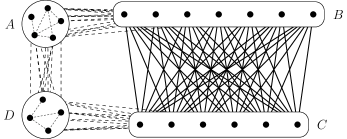
Figure 5: The partition $\{A,B,C,D\}$

From here the proof of Theorem 4 splits into two cases: $\varepsilon\leq\kappa/n$ and $\varepsilon\geq\kappa/n$, where $\kappa$ is a small absolute positive constant that will be determined (implicitly) later. The following proposition completes the proof when $\varepsilon$ is small.

Proposition 18.

Suppose that $\varepsilon\leq\kappa/n$ for a sufficiently small absolute constant $\kappa>0$. Then $G\cong G(a,b,c)$ for some $a,b,c$.

If $\varepsilon$ is large, we first obtain sharp estimates for the sizes of the sets $A,B,C,D$.

Proposition 19.

Let $G$ and $A,B,C,D$ satisfy the conclusions of Proposition 17 and suppose that $|B|\geq|C|$ and that $\varepsilon\geq\kappa/n$ for some constant $\kappa>0$. Then

$$|A\cup D| =\left(\mathchoice{{\hbox{$\displaystyle\sqrt{2\varepsilon\,}$}\lower 0.4pt\hbox{\vrule height=6.44444pt,depth=-5.15558pt}}}{{\hbox{$\textstyle\sqrt{2\varepsilon\,}$}\lower 0.4pt\hbox{\vrule height=6.44444pt,depth=-5.15558pt}}}{{\hbox{$\scriptstyle\sqrt{2\varepsilon\,}$}\lower 0.4pt\hbox{\vrule height=4.51111pt,depth=-3.6089pt}}}{{\hbox{$\scriptscriptstyle\sqrt{2\varepsilon\,}$}\lower 0.4pt\hbox{\vrule height=3.22221pt,depth=-2.57779pt}}}+O_{\kappa}(\varepsilon)\right)n,$$

$$|B| =\left(\frac{1}{2}-O_{\kappa}(\varepsilon^{3/4})\right)n,$$

$$|C| =\left(\frac{1}{2}-\mathchoice{{\hbox{$\displaystyle\sqrt{2\varepsilon\,}$}\lower 0.4pt\hbox{\vrule height=6.44444pt,depth=-5.15558pt}}}{{\hbox{$\textstyle\sqrt{2\varepsilon\,}$}\lower 0.4pt\hbox{\vrule height=6.44444pt,depth=-5.15558pt}}}{{\hbox{$\scriptstyle\sqrt{2\varepsilon\,}$}\lower 0.4pt\hbox{\vrule height=4.51111pt,depth=-3.6089pt}}}{{\hbox{$\scriptscriptstyle\sqrt{2\varepsilon\,}$}\lower 0.4pt\hbox{\vrule height=3.22221pt,depth=-2.57779pt}}}+O_{\kappa}(\varepsilon^{3/4})\right)n.$$

The next proposition completes the proof of Theorem 4 in the case where $\varepsilon$ is large.

Proposition 20.

Suppose that $\varepsilon\geq\kappa/n$ for some absolute constant $\kappa>0$. Then $G\cong G(a,b,c)$ for some $a,b,c$.

• Theorem 4 immediately follows from Propositions 17, 18, 19 and 20. The only minor technicality is that when we replace a graph with at most $(1/4+\delta)n^{2}$ edges by an optimal graph, we may increase the number of edges and lose this condition. However, Lemma 13 implies that the number of edges can increase by at most $O(n)$, so the condition is satisfied with a slightly relaxed value of $\delta$. ∎

The rest of this section is devoted to the proofs of Propositions 17, 18, 19 and 20, each of which is proved in a separate subsection.

4.1 Structure of an optimal graph

In this subsection, we prove Proposition 17 (see also Figure 5).

See 17

The first assertion follows fairly easily from the fact that the number of non-triangular edges is almost $n^{2}/4$. To complete the proof we use basic properties of optimal graphs.

• Let $H$ be the subgraph of $G$ whose edges are the non-triangular edges of $G$. We note that $H$ is a triangle-free graph with close to $n^{2}/4$ edges, which implies that $H$ is close to being a complete bipartite graph. This enables us to find independent (with respect to $G$) sets $U$ and $W$ of size almost $n/2$ each, such that $H$ contains almost all of the possible edges between them.

  Claim 21.

  There exist disjoint independent sets $U,W\subseteq V(G)$ such that every vertex in $U$ has at least $(1/2-O(\varepsilon^{1/4}))n$ non-triangular neighbours in $W$ and vice versa. In particular, $|U|,|W|\geq(1/2-O(\varepsilon^{1/4}))n$.

• Inequality (8) states that $e(H)=t(G)\geq(1/4-c\mathchoice{{\hbox{$\displaystyle\sqrt{\varepsilon\,}$}\lower 0.4pt\hbox{\vrule height=4.30554pt,depth=-3.44446pt}}}{{\hbox{$\textstyle\sqrt{\varepsilon\,}$}\lower 0.4pt\hbox{\vrule height=4.30554pt,depth=-3.44446pt}}}{{\hbox{$\scriptstyle\sqrt{\varepsilon\,}$}\lower 0.4pt\hbox{\vrule height=3.01389pt,depth=-2.41113pt}}}{{\hbox{$\scriptscriptstyle\sqrt{\varepsilon\,}$}\lower 0.4pt\hbox{\vrule height=2.15277pt,depth=-1.72223pt}}})n^{2}$ for some absolute constant $c$. From this we deduce that there are at most $2d\varepsilon^{1/4}$ vertices in $H$ of degree smaller than $(1/2-d\varepsilon^{1/4})n$ where $d=\mathchoice{{\hbox{$\displaystyle\sqrt{c\,}$}\lower 0.4pt\hbox{\vrule height=4.30554pt,depth=-3.44446pt}}}{{\hbox{$\textstyle\sqrt{c\,}$}\lower 0.4pt\hbox{\vrule height=4.30554pt,depth=-3.44446pt}}}{{\hbox{$\scriptstyle\sqrt{c\,}$}\lower 0.4pt\hbox{\vrule height=3.01389pt,depth=-2.41113pt}}}{{\hbox{$\scriptscriptstyle\sqrt{c\,}$}\lower 0.4pt\hbox{\vrule height=2.15277pt,depth=-1.72223pt}}}$. Indeed, suppose that we can find a set $S$ consisting of exactly $2d\varepsilon^{1/4}n$ vertices of degree smaller than $(1/2-d\varepsilon^{1/4})n$ in $H$. Since $H$ is triangle-free, $e(H\setminus S)\leq(n-|S|)^{2}/4$. Hence,

  $$e(H)\, <\,\frac{\left(n-|S|\right)^{2}}{4}+|S|\left(\frac{1}{2}-d\varepsilon^{1/4}\right)n$$

  $$=\,\frac{n^{2}}{4}-|S|\left(d\varepsilon^{1/4}n-\frac{|S|}{4}\right)$$

  $$=\,\left(\frac{1}{4}-d^{2}\mathchoice{{\hbox{$\displaystyle\sqrt{\varepsilon\,}$}\lower 0.4pt\hbox{\vrule height=4.30554pt,depth=-3.44446pt}}}{{\hbox{$\textstyle\sqrt{\varepsilon\,}$}\lower 0.4pt\hbox{\vrule height=4.30554pt,depth=-3.44446pt}}}{{\hbox{$\scriptstyle\sqrt{\varepsilon\,}$}\lower 0.4pt\hbox{\vrule height=3.01389pt,depth=-2.41113pt}}}{{\hbox{$\scriptscriptstyle\sqrt{\varepsilon\,}$}\lower 0.4pt\hbox{\vrule height=2.15277pt,depth=-1.72223pt}}}\right)n^{2}$$

  $$=\,\left(\frac{1}{4}-c\mathchoice{{\hbox{$\displaystyle\sqrt{\varepsilon\,}$}\lower 0.4pt\hbox{\vrule height=4.30554pt,depth=-3.44446pt}}}{{\hbox{$\textstyle\sqrt{\varepsilon\,}$}\lower 0.4pt\hbox{\vrule height=4.30554pt,depth=-3.44446pt}}}{{\hbox{$\scriptstyle\sqrt{\varepsilon\,}$}\lower 0.4pt\hbox{\vrule height=3.01389pt,depth=-2.41113pt}}}{{\hbox{$\scriptscriptstyle\sqrt{\varepsilon\,}$}\lower 0.4pt\hbox{\vrule height=2.15277pt,depth=-1.72223pt}}}\right)n^{2},$$

  a contradiction.

  Let $u\in V(H)$ be any vertex with $\deg_{H}(u)\geq(1/2-d\varepsilon^{1/4})n$. Denote by $U$ the set of vertices in $N_{H}(u)$ that have at least $(1/2-d\varepsilon^{1/4})n$ neighbours in $H$. Since the edges of $H$ are non-triangular in $G$, it follows that $U$ is independent in $G$. Moreover, $|U|\geq\deg_{H}(u)-2d\varepsilon^{1/4}n\geq(1/2-O(\varepsilon^{1/4}))n$.

  Now let $v\in U$ and denote by $W$ the set of vertices in $N_{H}(v)$ whose degree in $H$ is at least $(1/2-d\varepsilon^{1/4})n$. As before, $W$ is independent in $G$ and has size at least $(1/2-O(\varepsilon^{1/4}))n$. Finally, every vertex in $U$ has at least $(1/2-d\varepsilon^{1/4})n-(n-|U|-|W|)\geq(1/2-O(\varepsilon^{1/4}))n$ non-triangular neighbours in $W$, and vice versa. ∎

Let $U$ and $W$ be the disjoint independent sets given Claim 21. The following similar claim, allows us to enlarge $U$ and $W$ to obtain sets $B$ and $C$ which will be shown to satisfy the requirements of Proposition 17.

Claim 22.

There exist disjoint independent sets $B,C\subseteq V(G)$, satisfying $U\subseteq B$ and $W\subseteq C$ and $|B\cup C|\geq(1-O(\mathchoice{{\hbox{$\displaystyle\sqrt{\varepsilon\,}$}\lower 0.4pt\hbox{\vrule height=4.30554pt,depth=-3.44446pt}}}{{\hbox{$\textstyle\sqrt{\varepsilon\,}$}\lower 0.4pt\hbox{\vrule height=4.30554pt,depth=-3.44446pt}}}{{\hbox{$\scriptstyle\sqrt{\varepsilon\,}$}\lower 0.4pt\hbox{\vrule height=3.01389pt,depth=-2.41113pt}}}{{\hbox{$\scriptscriptstyle\sqrt{\varepsilon\,}$}\lower 0.4pt\hbox{\vrule height=2.15277pt,depth=-1.72223pt}}}))n$, such that every vertex in $B$ has at least $2n/5$ non-triangular neighbours in $C$ and vice versa.

• We first show that there are at most $O(\mathchoice{{\hbox{$\displaystyle\sqrt{\varepsilon\,}$}\lower 0.4pt\hbox{\vrule height=4.30554pt,depth=-3.44446pt}}}{{\hbox{$\textstyle\sqrt{\varepsilon\,}$}\lower 0.4pt\hbox{\vrule height=4.30554pt,depth=-3.44446pt}}}{{\hbox{$\scriptstyle\sqrt{\varepsilon\,}$}\lower 0.4pt\hbox{\vrule height=3.01389pt,depth=-2.41113pt}}}{{\hbox{$\scriptscriptstyle\sqrt{\varepsilon\,}$}\lower 0.4pt\hbox{\vrule height=2.15277pt,depth=-1.72223pt}}}n)$ vertices of degree at most $21n/50$ in $H$. To this end we recall Inequality (8), which states that $e(H)=t(G)\geq(1/4-c\mathchoice{{\hbox{$\displaystyle\sqrt{\varepsilon\,}$}\lower 0.4pt\hbox{\vrule height=4.30554pt,depth=-3.44446pt}}}{{\hbox{$\textstyle\sqrt{\varepsilon\,}$}\lower 0.4pt\hbox{\vrule height=4.30554pt,depth=-3.44446pt}}}{{\hbox{$\scriptstyle\sqrt{\varepsilon\,}$}\lower 0.4pt\hbox{\vrule height=3.01389pt,depth=-2.41113pt}}}{{\hbox{$\scriptscriptstyle\sqrt{\varepsilon\,}$}\lower 0.4pt\hbox{\vrule height=2.15277pt,depth=-1.72223pt}}})n$ for some absolute constant $c$. Importantly, this constant does not depend on $\delta$, so we may choose $\delta$ to satisfy $c\mathchoice{{\hbox{$\displaystyle\sqrt{\delta\,}$}\lower 0.4pt\hbox{\vrule height=6.94444pt,depth=-5.55559pt}}}{{\hbox{$\textstyle\sqrt{\delta\,}$}\lower 0.4pt\hbox{\vrule height=6.94444pt,depth=-5.55559pt}}}{{\hbox{$\scriptstyle\sqrt{\delta\,}$}\lower 0.4pt\hbox{\vrule height=4.8611pt,depth=-3.8889pt}}}{{\hbox{$\scriptscriptstyle\sqrt{\delta\,}$}\lower 0.4pt\hbox{\vrule height=3.47221pt,depth=-2.77779pt}}}\leq 1/100$. Recall that $\delta$ is an upper bound for $\varepsilon$, so we have $c\mathchoice{{\hbox{$\displaystyle\sqrt{\varepsilon\,}$}\lower 0.4pt\hbox{\vrule height=4.30554pt,depth=-3.44446pt}}}{{\hbox{$\textstyle\sqrt{\varepsilon\,}$}\lower 0.4pt\hbox{\vrule height=4.30554pt,depth=-3.44446pt}}}{{\hbox{$\scriptstyle\sqrt{\varepsilon\,}$}\lower 0.4pt\hbox{\vrule height=3.01389pt,depth=-2.41113pt}}}{{\hbox{$\scriptscriptstyle\sqrt{\varepsilon\,}$}\lower 0.4pt\hbox{\vrule height=2.15277pt,depth=-1.72223pt}}}\leq 1/100$.

  Suppose that $S$ is a set consisting of exactly $25c\mathchoice{{\hbox{$\displaystyle\sqrt{\varepsilon\,}$}\lower 0.4pt\hbox{\vrule height=4.30554pt,depth=-3.44446pt}}}{{\hbox{$\textstyle\sqrt{\varepsilon\,}$}\lower 0.4pt\hbox{\vrule height=4.30554pt,depth=-3.44446pt}}}{{\hbox{$\scriptstyle\sqrt{\varepsilon\,}$}\lower 0.4pt\hbox{\vrule height=3.01389pt,depth=-2.41113pt}}}{{\hbox{$\scriptscriptstyle\sqrt{\varepsilon\,}$}\lower 0.4pt\hbox{\vrule height=2.15277pt,depth=-1.72223pt}}}n$ vertices of degree at most $21n/50$ in $H$. Then, similarly to the previous claim,

  $$e(H) \leq\frac{\left(n-|S|\right)^{2}}{4}+|S|\frac{21n}{50}$$

  $$=\frac{n^{2}}{4}-|S|\left(\frac{4n}{25}-\frac{|S|}{4}\right)$$

  $$<\left(\frac{1}{4}-2c\mathchoice{{\hbox{$\displaystyle\sqrt{\varepsilon\,}$}\lower 0.4pt\hbox{\vrule height=4.30554pt,depth=-3.44446pt}}}{{\hbox{$\textstyle\sqrt{\varepsilon\,}$}\lower 0.4pt\hbox{\vrule height=4.30554pt,depth=-3.44446pt}}}{{\hbox{$\scriptstyle\sqrt{\varepsilon\,}$}\lower 0.4pt\hbox{\vrule height=3.01389pt,depth=-2.41113pt}}}{{\hbox{$\scriptscriptstyle\sqrt{\varepsilon\,}$}\lower 0.4pt\hbox{\vrule height=2.15277pt,depth=-1.72223pt}}}\right)n^{2},$$

  a contradiction to Inequality (8). Therefore, there are at most $O(\mathchoice{{\hbox{$\displaystyle\sqrt{\varepsilon\,}$}\lower 0.4pt\hbox{\vrule height=4.30554pt,depth=-3.44446pt}}}{{\hbox{$\textstyle\sqrt{\varepsilon\,}$}\lower 0.4pt\hbox{\vrule height=4.30554pt,depth=-3.44446pt}}}{{\hbox{$\scriptstyle\sqrt{\varepsilon\,}$}\lower 0.4pt\hbox{\vrule height=3.01389pt,depth=-2.41113pt}}}{{\hbox{$\scriptscriptstyle\sqrt{\varepsilon\,}$}\lower 0.4pt\hbox{\vrule height=2.15277pt,depth=-1.72223pt}}}n)$ vertices with degree at most $21n/50$ in $H$.

  Recall that every vertex in $U$ has at least $(1/2-O(\varepsilon^{1/4}))n\geq 2n/5$ non-triangular neighbours in $W$ and vice versa. Here we implicitly assume that $\delta$ is small enough to make this inequality true, and we shall do so throughout this proof.

  Denote by $X$ the set of vertices in $V(G)\setminus(U\cup W)$ whose degree in $H$ is at least $21n/50$. We note that no vertex in $X$ has neighbours in both $U$ and $W$. Indeed, suppose that $v\in X$ is adjacent to $u\in U$ and $w\in W$. Since $v$ is not adjacent to any non-triangular neighbour of either $u$ or $w$, it has at most $O(\varepsilon^{1/4}n)$ neighbours in $U$ and at most $O(\varepsilon^{1/4}n)$ neighbours in $W$, implying that $\deg_{H}(v)\leq O(\varepsilon^{1/4}n)$, a contradiction to the assumption that $\deg_{H}(v)\geq 21n/50$.

  Let $Y$ be the set of vertices in $X$ that are adjacent to vertices in $U$ and, similarly, let $Z$ be the set of vertices in $X$ that have neighbours in $W$. Then every vertex in $Y$ has at least $21/50n-O(\varepsilon^{1/4}n)\geq 2n/5$ non-triangular neighbours in $U$ and no neighbours in $W$. In particular, since $|U|\leq n-|W|<4n/5$, any two vertices in $Y$ share a non-triangular neighbour in $U$, hence $Y$ is an independent set in $G$. Denote $B=Y\cup W$ and $C=Z\cup U$. Then $B$ and $C$ are independent sets, such that every vertex in $B$ has at least $2n/5$ non-triangular neighbours in $C$, and vice versa. Furthermore, $|B\cup C|=|V(G)\setminus X|\geq(1-O(\mathchoice{{\hbox{$\displaystyle\sqrt{\varepsilon\,}$}\lower 0.4pt\hbox{\vrule height=4.30554pt,depth=-3.44446pt}}}{{\hbox{$\textstyle\sqrt{\varepsilon\,}$}\lower 0.4pt\hbox{\vrule height=4.30554pt,depth=-3.44446pt}}}{{\hbox{$\scriptstyle\sqrt{\varepsilon\,}$}\lower 0.4pt\hbox{\vrule height=3.01389pt,depth=-2.41113pt}}}{{\hbox{$\scriptscriptstyle\sqrt{\varepsilon\,}$}\lower 0.4pt\hbox{\vrule height=2.15277pt,depth=-1.72223pt}}}))n$, so the proof of Claim 22 is complete. ∎

We can now finish the proof of Proposition 17. Let $B$ and $C$ be as in Claim 22. Since every vertex in $B\cup C$ has at least $2n/5$ non-triangular neighbours, it follows from Observation 8 and the assumption that $G$ is optimal that every vertex in $G$ has degree at least $2n/5-1$. We conclude (similarly to the proof of Claim 22) that no vertex in $G$ has neighbours in both $B$ and $C$. Indeed, suppose that some $v\in V(G)$ is adjacent to some $u\in B$ and $w\in C$. Since $u$ has at least $2n/5$ non-triangular neighbours in $C$, $v$ is adjacent to at most $|C|-2n/5$ vertices in $C$ and, similarly, to at most $|B|-2n/5$ vertices in $B$. It follows that $u$ has degree at most $n/5$, a contradiction.

Since no vertex in $G$ is adjacent to a vertex in $B$ and a vertex in $C$, we may add all missing edges between $B$ and $C$ without creating new triangles. However, $G$ is an optimal graph, so in fact all edges between $B$ and $C$ are present in $G$. Again, since vertices in $B$ and $C$ do not have common neighbours, all edges between $B$ and $C$ are non-triangular.

We may assume that $|B|\geq|C|$. Then $|B|\geq(1/2-O(\mathchoice{{\hbox{$\displaystyle\sqrt{\varepsilon\,}$}\lower 0.4pt\hbox{\vrule height=4.30554pt,depth=-3.44446pt}}}{{\hbox{$\textstyle\sqrt{\varepsilon\,}$}\lower 0.4pt\hbox{\vrule height=4.30554pt,depth=-3.44446pt}}}{{\hbox{$\scriptstyle\sqrt{\varepsilon\,}$}\lower 0.4pt\hbox{\vrule height=3.01389pt,depth=-2.41113pt}}}{{\hbox{$\scriptscriptstyle\sqrt{\varepsilon\,}$}\lower 0.4pt\hbox{\vrule height=2.15277pt,depth=-1.72223pt}}}))n$ and hence every vertex in $C$ has non-triangular degree at least $(1/2-O(\mathchoice{{\hbox{$\displaystyle\sqrt{\varepsilon\,}$}\lower 0.4pt\hbox{\vrule height=4.30554pt,depth=-3.44446pt}}}{{\hbox{$\textstyle\sqrt{\varepsilon\,}$}\lower 0.4pt\hbox{\vrule height=4.30554pt,depth=-3.44446pt}}}{{\hbox{$\scriptstyle\sqrt{\varepsilon\,}$}\lower 0.4pt\hbox{\vrule height=3.01389pt,depth=-2.41113pt}}}{{\hbox{$\scriptscriptstyle\sqrt{\varepsilon\,}$}\lower 0.4pt\hbox{\vrule height=2.15277pt,depth=-1.72223pt}}}))n$. Again, by Observation 8, every vertex in $G$ has degree at least $(1/2-O(\mathchoice{{\hbox{$\displaystyle\sqrt{\varepsilon\,}$}\lower 0.4pt\hbox{\vrule height=4.30554pt,depth=-3.44446pt}}}{{\hbox{$\textstyle\sqrt{\varepsilon\,}$}\lower 0.4pt\hbox{\vrule height=4.30554pt,depth=-3.44446pt}}}{{\hbox{$\scriptstyle\sqrt{\varepsilon\,}$}\lower 0.4pt\hbox{\vrule height=3.01389pt,depth=-2.41113pt}}}{{\hbox{$\scriptscriptstyle\sqrt{\varepsilon\,}$}\lower 0.4pt\hbox{\vrule height=2.15277pt,depth=-1.72223pt}}}))n$. Since $B$ is an independent set, it follows that $n-|B|\geq(1/2-O(\mathchoice{{\hbox{$\displaystyle\sqrt{\varepsilon\,}$}\lower 0.4pt\hbox{\vrule height=4.30554pt,depth=-3.44446pt}}}{{\hbox{$\textstyle\sqrt{\varepsilon\,}$}\lower 0.4pt\hbox{\vrule height=4.30554pt,depth=-3.44446pt}}}{{\hbox{$\scriptstyle\sqrt{\varepsilon\,}$}\lower 0.4pt\hbox{\vrule height=3.01389pt,depth=-2.41113pt}}}{{\hbox{$\scriptscriptstyle\sqrt{\varepsilon\,}$}\lower 0.4pt\hbox{\vrule height=2.15277pt,depth=-1.72223pt}}}))n$. Therefore $|C|=|B\cup C|-|B|\geq(1/2-O(\mathchoice{{\hbox{$\displaystyle\sqrt{\varepsilon\,}$}\lower 0.4pt\hbox{\vrule height=4.30554pt,depth=-3.44446pt}}}{{\hbox{$\textstyle\sqrt{\varepsilon\,}$}\lower 0.4pt\hbox{\vrule height=4.30554pt,depth=-3.44446pt}}}{{\hbox{$\scriptstyle\sqrt{\varepsilon\,}$}\lower 0.4pt\hbox{\vrule height=3.01389pt,depth=-2.41113pt}}}{{\hbox{$\scriptscriptstyle\sqrt{\varepsilon\,}$}\lower 0.4pt\hbox{\vrule height=2.15277pt,depth=-1.72223pt}}}))n$.

We are now done with the first assertion of Proposition 17, and the remaining ones follow easily. Let $A$ be the set of vertices outside of $B\cup C$ that are adjacent to a vertex in $B$ and, similarly, let $D$ be the set of vertices outside of $B\cup C$ that have a neighbour in $C$. Then $\{A,B,C,D\}$ forms a partition of $G$, because a vertex without neighbours in $B\cup C$ would have too small a degree. This establishes the second assertion.

To prove the third assertion, we may assume that every vertex in $A$ has a neighbour in $A$: if some $u\in A$ has no neighbours in $A$, then we may add all edges between $u$ and the vertices in $B$ without creating new triangles and then reassign $u$ to $C$. Similarly, we may assume that every vertex in $D$ has a neighbour in $D$.

By inspecting the degrees, any two vertices in $A$ have a common neighbour in $B$. Therefore there cannot be any non-triangular edges with both ends in $A$ or, similarly, with both ends in $D$. It remains to conclude that every vertex in $A\cup D$ is incident with at most $O(\mathchoice{{\hbox{$\displaystyle\sqrt{\varepsilon\,}$}\lower 0.4pt\hbox{\vrule height=4.30554pt,depth=-3.44446pt}}}{{\hbox{$\textstyle\sqrt{\varepsilon\,}$}\lower 0.4pt\hbox{\vrule height=4.30554pt,depth=-3.44446pt}}}{{\hbox{$\scriptstyle\sqrt{\varepsilon\,}$}\lower 0.4pt\hbox{\vrule height=3.01389pt,depth=-2.41113pt}}}{{\hbox{$\scriptscriptstyle\sqrt{\varepsilon\,}$}\lower 0.4pt\hbox{\vrule height=2.15277pt,depth=-1.72223pt}}}n)$ non-triangular edges. Let $u\in A$ and let $v\in A$ by a neighbour of $u$. Since $u$ and $v$ have neighbours only in $A\cup D\cup B$ and the degree of $v$ is at least $(1/2-O(\mathchoice{{\hbox{$\displaystyle\sqrt{\varepsilon\,}$}\lower 0.4pt\hbox{\vrule height=4.30554pt,depth=-3.44446pt}}}{{\hbox{$\textstyle\sqrt{\varepsilon\,}$}\lower 0.4pt\hbox{\vrule height=4.30554pt,depth=-3.44446pt}}}{{\hbox{$\scriptstyle\sqrt{\varepsilon\,}$}\lower 0.4pt\hbox{\vrule height=3.01389pt,depth=-2.41113pt}}}{{\hbox{$\scriptscriptstyle\sqrt{\varepsilon\,}$}\lower 0.4pt\hbox{\vrule height=2.15277pt,depth=-1.72223pt}}}))n$, it follows that $u$ has at most $|A\cup D\cup B|-(1/2-O(\mathchoice{{\hbox{$\displaystyle\sqrt{\varepsilon\,}$}\lower 0.4pt\hbox{\vrule height=4.30554pt,depth=-3.44446pt}}}{{\hbox{$\textstyle\sqrt{\varepsilon\,}$}\lower 0.4pt\hbox{\vrule height=4.30554pt,depth=-3.44446pt}}}{{\hbox{$\scriptstyle\sqrt{\varepsilon\,}$}\lower 0.4pt\hbox{\vrule height=3.01389pt,depth=-2.41113pt}}}{{\hbox{$\scriptscriptstyle\sqrt{\varepsilon\,}$}\lower 0.4pt\hbox{\vrule height=2.15277pt,depth=-1.72223pt}}}))n=O(\mathchoice{{\hbox{$\displaystyle\sqrt{\varepsilon\,}$}\lower 0.4pt\hbox{\vrule height=4.30554pt,depth=-3.44446pt}}}{{\hbox{$\textstyle\sqrt{\varepsilon\,}$}\lower 0.4pt\hbox{\vrule height=4.30554pt,depth=-3.44446pt}}}{{\hbox{$\scriptstyle\sqrt{\varepsilon\,}$}\lower 0.4pt\hbox{\vrule height=3.01389pt,depth=-2.41113pt}}}{{\hbox{$\scriptscriptstyle\sqrt{\varepsilon\,}$}\lower 0.4pt\hbox{\vrule height=2.15277pt,depth=-1.72223pt}}}n)$ non-triangular neighbours. The same holds for any vertex in $D$. This establishes the fourth assertion and completes the proof of Proposition 17. ∎

4.2 Completing the proof if $\varepsilon n$ is small

We now prove Proposition 18, which completes the proof of Theorem 4 in case $\varepsilon$ is small.

See 18

• It follows from the assumptions on the sets $A,B,C,D$ that $|A\cup D|=O(\mathchoice{{\hbox{$\displaystyle\sqrt{\varepsilon\,}$}\lower 0.4pt\hbox{\vrule height=4.30554pt,depth=-3.44446pt}}}{{\hbox{$\textstyle\sqrt{\varepsilon\,}$}\lower 0.4pt\hbox{\vrule height=4.30554pt,depth=-3.44446pt}}}{{\hbox{$\scriptstyle\sqrt{\varepsilon\,}$}\lower 0.4pt\hbox{\vrule height=3.01389pt,depth=-2.41113pt}}}{{\hbox{$\scriptscriptstyle\sqrt{\varepsilon\,}$}\lower 0.4pt\hbox{\vrule height=2.15277pt,depth=-1.72223pt}}}n)$ and that each vertex in $A\cup D$ is incident with at most $O(\mathchoice{{\hbox{$\displaystyle\sqrt{\varepsilon\,}$}\lower 0.4pt\hbox{\vrule height=4.30554pt,depth=-3.44446pt}}}{{\hbox{$\textstyle\sqrt{\varepsilon\,}$}\lower 0.4pt\hbox{\vrule height=4.30554pt,depth=-3.44446pt}}}{{\hbox{$\scriptstyle\sqrt{\varepsilon\,}$}\lower 0.4pt\hbox{\vrule height=3.01389pt,depth=-2.41113pt}}}{{\hbox{$\scriptscriptstyle\sqrt{\varepsilon\,}$}\lower 0.4pt\hbox{\vrule height=2.15277pt,depth=-1.72223pt}}}n)$ non-triangular edges. Therefore the number of non-triangular edges with an end in $A\cup D$ is $O(\varepsilon n^{2})=O(\kappa n)$. We show that, in fact, there are no such edges.

  Suppose that $uv$ is a non-triangular edge with $u\in A\cup D$. Without loss of generality, we may assume that $u\in A$ and $v\in B\cup D$. Observe that the neighbours of $u$ are not adjacent to $v$. Let $G^{\prime}$ be the graph obtained by adding the edges between $v$ and the neighbours of $u$ in $A$, removing the edges between $u$ and $A\setminus\{u\}$ and also adding all missing edges between $u$ and $B$. Then $e(G^{\prime})\geq e(G)$ and $t(G^{\prime})\geq t(G)+|B|-O(\kappa n)>t(G)$, where the last inequality holds provided that we choose $\kappa$ small enough. However, this contradicts the optimality of $G$, so there cannot be such an edge $uv$.

  It is now easy to finish the proof. By what we have just proved, all the missing edges with both ends in $A\cup D$ may be added without causing a non-triangular edge to become triangular, i.e., $A\cup D$ is a clique. We may assume that $|B|\geq|C|$. Remove the edges between $D$ and $C$ and add all possible edges between $D$ and $B$. The result is a graph which is isomorphic to $G(|A\cup D|,|B|,|C|)$, with at least as many edges and non-triangular edges as $G$. ∎

4.3 Sizes of $A,B,C,D$

In this subsection we prepare for the proof of Theorem 4 in the case where $\varepsilon n$ is large. In particular, we obtain good bounds for the sizes of the sets $A\cup D$, $B$ and $C$.

See 19

The proof is fairly technical, and its main tool is the lower bound on $t(G)$ from Inequality (7).

• Denote $a=|A\cup D|$, $b=|B|$ and $c=|C|$ and write

  $$a =\left(\mathchoice{{\hbox{$\displaystyle\sqrt{2\varepsilon\,}$}\lower 0.4pt\hbox{\vrule height=6.44444pt,depth=-5.15558pt}}}{{\hbox{$\textstyle\sqrt{2\varepsilon\,}$}\lower 0.4pt\hbox{\vrule height=6.44444pt,depth=-5.15558pt}}}{{\hbox{$\scriptstyle\sqrt{2\varepsilon\,}$}\lower 0.4pt\hbox{\vrule height=4.51111pt,depth=-3.6089pt}}}{{\hbox{$\scriptscriptstyle\sqrt{2\varepsilon\,}$}\lower 0.4pt\hbox{\vrule height=3.22221pt,depth=-2.57779pt}}}+\alpha\right)n,$$

  $$b =\left(\frac{1}{2}-\beta\right)n,$$

  $$c =\left(\frac{1}{2}-\mathchoice{{\hbox{$\displaystyle\sqrt{2\varepsilon\,}$}\lower 0.4pt\hbox{\vrule height=6.44444pt,depth=-5.15558pt}}}{{\hbox{$\textstyle\sqrt{2\varepsilon\,}$}\lower 0.4pt\hbox{\vrule height=6.44444pt,depth=-5.15558pt}}}{{\hbox{$\scriptstyle\sqrt{2\varepsilon\,}$}\lower 0.4pt\hbox{\vrule height=4.51111pt,depth=-3.6089pt}}}{{\hbox{$\scriptscriptstyle\sqrt{2\varepsilon\,}$}\lower 0.4pt\hbox{\vrule height=3.22221pt,depth=-2.57779pt}}}+\beta-\alpha\right)n,$$

  where the quantities $\alpha$ and $\beta$ are defined by these identities. We cannot assume that $\alpha$ and $\beta$ are positive, but we have $-\mathchoice{{\hbox{$\displaystyle\sqrt{2\varepsilon\,}$}\lower 0.4pt\hbox{\vrule height=6.44444pt,depth=-5.15558pt}}}{{\hbox{$\textstyle\sqrt{2\varepsilon\,}$}\lower 0.4pt\hbox{\vrule height=6.44444pt,depth=-5.15558pt}}}{{\hbox{$\scriptstyle\sqrt{2\varepsilon\,}$}\lower 0.4pt\hbox{\vrule height=4.51111pt,depth=-3.6089pt}}}{{\hbox{$\scriptscriptstyle\sqrt{2\varepsilon\,}$}\lower 0.4pt\hbox{\vrule height=3.22221pt,depth=-2.57779pt}}}\leq\alpha\leq O(\mathchoice{{\hbox{$\displaystyle\sqrt{\varepsilon\,}$}\lower 0.4pt\hbox{\vrule height=4.30554pt,depth=-3.44446pt}}}{{\hbox{$\textstyle\sqrt{\varepsilon\,}$}\lower 0.4pt\hbox{\vrule height=4.30554pt,depth=-3.44446pt}}}{{\hbox{$\scriptstyle\sqrt{\varepsilon\,}$}\lower 0.4pt\hbox{\vrule height=3.01389pt,depth=-2.41113pt}}}{{\hbox{$\scriptscriptstyle\sqrt{\varepsilon\,}$}\lower 0.4pt\hbox{\vrule height=2.15277pt,depth=-1.72223pt}}})$, where the second inequality comes from Proposition 17. Since there are at most $O(\varepsilon n^{2})$ non-triangular edges with an end in $A\cup D$, we have

  $$t(G)\, \leq\,bc+O(\varepsilon n^{2})$$

  $$\leq\,\frac{(n-a)^{2}}{4}+O(\varepsilon n^{2})$$

  $$\leq\,\frac{n^{2}}{4}-\frac{an}{2}+O(\varepsilon n^{2}).$$

  Combining this with Inequality (7), which states that $t(G)\geq\left(1/4-\mathchoice{{\hbox{$\displaystyle\sqrt{\varepsilon/2\,}$}\lower 0.4pt\hbox{\vrule height=7.5pt,depth=-6.00003pt}}}{{\hbox{$\textstyle\sqrt{\varepsilon/2\,}$}\lower 0.4pt\hbox{\vrule height=7.5pt,depth=-6.00003pt}}}{{\hbox{$\scriptstyle\sqrt{\varepsilon/2\,}$}\lower 0.4pt\hbox{\vrule height=5.25pt,depth=-4.20003pt}}}{{\hbox{$\scriptscriptstyle\sqrt{\varepsilon/2\,}$}\lower 0.4pt\hbox{\vrule height=3.75pt,depth=-3.00002pt}}}-O(1/n)\right)n^{2}$ , we get

  $$\frac{1}{4}-\mathchoice{{\hbox{$\displaystyle\sqrt{\frac{\varepsilon}{2}\,}$}\lower 0.4pt\hbox{\vrule height=7.52776pt,depth=-6.02223pt}}}{{\hbox{$\textstyle\sqrt{\frac{\varepsilon}{2}\,}$}\lower 0.4pt\hbox{\vrule height=5.26944pt,depth=-4.21558pt}}}{{\hbox{$\scriptstyle\sqrt{\frac{\varepsilon}{2}\,}$}\lower 0.4pt\hbox{\vrule height=3.76387pt,depth=-3.01111pt}}}{{\hbox{$\scriptscriptstyle\sqrt{\frac{\varepsilon}{2}\,}$}\lower 0.4pt\hbox{\vrule height=3.76387pt,depth=-3.01111pt}}}-O_{\kappa}(\varepsilon)\;\leq\;\frac{t(G)}{n^{2}}\;\leq\;\frac{1}{4}-\frac{(\mathchoice{{\hbox{$\displaystyle\sqrt{2\varepsilon\,}$}\lower 0.4pt\hbox{\vrule height=6.44444pt,depth=-5.15558pt}}}{{\hbox{$\textstyle\sqrt{2\varepsilon\,}$}\lower 0.4pt\hbox{\vrule height=6.44444pt,depth=-5.15558pt}}}{{\hbox{$\scriptstyle\sqrt{2\varepsilon\,}$}\lower 0.4pt\hbox{\vrule height=4.51111pt,depth=-3.6089pt}}}{{\hbox{$\scriptscriptstyle\sqrt{2\varepsilon\,}$}\lower 0.4pt\hbox{\vrule height=3.22221pt,depth=-2.57779pt}}}+\alpha)}{2}+O(\varepsilon).$$

  Therefore $\alpha=O_{\kappa}(\varepsilon)$. Using the fact that $b\geq c$ and that any vertex in $A\cup D$ sends edges to only one of $B$ and $C$, we obtain the following upper bound on the number of edges in $G$.

  $$e(G) \leq b(n-b)+a^{2}/2.$$

  Combining this with the definition $e(G)=(1/4+\varepsilon)n^{2}$, we get

  $$1/4+\varepsilon\, \leq\,\left(1/2-\beta\right)\left(1/2+\beta\right)+\frac{\left(\mathchoice{{\hbox{$\displaystyle\sqrt{2\varepsilon\,}$}\lower 0.4pt\hbox{\vrule height=6.44444pt,depth=-5.15558pt}}}{{\hbox{$\textstyle\sqrt{2\varepsilon\,}$}\lower 0.4pt\hbox{\vrule height=6.44444pt,depth=-5.15558pt}}}{{\hbox{$\scriptstyle\sqrt{2\varepsilon\,}$}\lower 0.4pt\hbox{\vrule height=4.51111pt,depth=-3.6089pt}}}{{\hbox{$\scriptscriptstyle\sqrt{2\varepsilon\,}$}\lower 0.4pt\hbox{\vrule height=3.22221pt,depth=-2.57779pt}}}+\alpha\right)^{2}}{2}$$

  $$=\,1/4-\beta^{2}+\varepsilon+\alpha(\mathchoice{{\hbox{$\displaystyle\sqrt{2\varepsilon\,}$}\lower 0.4pt\hbox{\vrule height=6.44444pt,depth=-5.15558pt}}}{{\hbox{$\textstyle\sqrt{2\varepsilon\,}$}\lower 0.4pt\hbox{\vrule height=6.44444pt,depth=-5.15558pt}}}{{\hbox{$\scriptstyle\sqrt{2\varepsilon\,}$}\lower 0.4pt\hbox{\vrule height=4.51111pt,depth=-3.6089pt}}}{{\hbox{$\scriptscriptstyle\sqrt{2\varepsilon\,}$}\lower 0.4pt\hbox{\vrule height=3.22221pt,depth=-2.57779pt}}}+\alpha/2)$$

  It follows that $\beta\leq\alpha(\mathchoice{{\hbox{$\displaystyle\sqrt{2\varepsilon\,}$}\lower 0.4pt\hbox{\vrule height=6.44444pt,depth=-5.15558pt}}}{{\hbox{$\textstyle\sqrt{2\varepsilon\,}$}\lower 0.4pt\hbox{\vrule height=6.44444pt,depth=-5.15558pt}}}{{\hbox{$\scriptstyle\sqrt{2\varepsilon\,}$}\lower 0.4pt\hbox{\vrule height=4.51111pt,depth=-3.6089pt}}}{{\hbox{$\scriptscriptstyle\sqrt{2\varepsilon\,}$}\lower 0.4pt\hbox{\vrule height=3.22221pt,depth=-2.57779pt}}}+\alpha/2)$. In particular, $\alpha\geq 0$ and $\beta=O_{\kappa}(\varepsilon^{3/4})$, implying that the assertions of Proposition 19 hold. ∎

4.4 Completing the proof if $\varepsilon n$ is large

We are now able to complete the proof of Theorem 4 under the assumption that $\varepsilon\geq\kappa/n$ for some absolute constant $\kappa>0$.

See 20

The proof consists of two stages. In the first stage we use the bounds from Proposition 19 to conclude that $D$ is very small and that the number of vertices in $A$ which are adjacent to a non-triangular edges is small. In the second stage, we show that if $D$ is non-empty or if there is a vertex in $A$ with a non-triangular neighbour then $G$ can be manipulated to obtain a graph with more edges and more non-triangular edges, contradicting the assumption that $G$ is optimal. It follows that $G$ is isomorphic to a graph $G(a,b,c)$.

• We start by showing that the edges between $B\cup D$ and $A\cup C$ form an almost complete bipartite subgraph. We shall be using the estimates on the size of the sets $A\cup D$, $B$ and $C$ from Proposition 19. Note that $\kappa$ is an absolute constant (determined implicitly in Proposition 18). Thus we may remove the dependence on $\kappa$ in the estimates of these sizes.

  Claim 23.

  Every vertex in $B\cup D$ is adjacent to all but $O(\varepsilon^{3/4}n)$ vertices in $A\cup C$. Furthermore, $|D|=O(\varepsilon^{3/4}n)$.

• The non-triangular degree of any vertex in $C$ is at least $|B|$. Hence by Observation 8 every vertex in $G$ has degree at least $|B|-1$. The vertices in $B\cup D$ are not adjacent to any vertex in $B$. Since $|B|\geq(1/2-O(\varepsilon^{3/4}))n$, it follows that every vertex in $B\cup D$ is adjacent to all but $O(\varepsilon^{3/4}n)$ vertices in $V(G)\setminus B=A\cup C\cup D$. Since there are no edges between $B$ and $D$, $|D|=O(\varepsilon^{3/4}n)$. ∎

Denote by $T$ the set of triangular vertices in $A$ (recall that a triangular vertex is incident only with triangular edges) and let $S=A\setminus T$. We show that the vertices in $S$ have few neighbours in $A$.

Claim 24.

Every vertex in $S$ has $O(\varepsilon^{3/4}n)$ neighbours in $A$.

• Let $u\in S$ and let $v$ be a non-triangular neighbour of $u$. Then $v\in B\cup D$, because there are no edges between $A$ and $C$, and there are no non-triangular edges with both ends in $A$. Recall that by Claim 23, $v$ is adjacent to all but $O(\varepsilon^{3/4}n)$ vertices in $A$. Since $uv$ is non-triangular, $u$ and $v$ have no common neighbours, implying that $u$ has $O(\varepsilon^{3/4}n)$ neighbours in $A$. ∎

We conclude that almost all of the vertices in $A$ are also in $T$.

Claim 25.

$|T|\geq(\mathchoice{{\hbox{$\displaystyle\sqrt{2\varepsilon\,}$}\lower 0.4pt\hbox{\vrule height=6.44444pt,depth=-5.15558pt}}}{{\hbox{$\textstyle\sqrt{2\varepsilon\,}$}\lower 0.4pt\hbox{\vrule height=6.44444pt,depth=-5.15558pt}}}{{\hbox{$\scriptstyle\sqrt{2\varepsilon\,}$}\lower 0.4pt\hbox{\vrule height=4.51111pt,depth=-3.6089pt}}}{{\hbox{$\scriptscriptstyle\sqrt{2\varepsilon\,}$}\lower 0.4pt\hbox{\vrule height=3.22221pt,depth=-2.57779pt}}}-O(\varepsilon^{3/4}))n^{2}$.

• By removing the edges with both ends in $A$ or in $D$ from $G$, we remain with a bipartite graph, so $(1/4+\varepsilon)n^{2}=e(G)\leq n^{2}/4+e(G[A])+e(G[D])$. Since $|D|=O(\varepsilon^{3/4}n)$, we have $e(G[D])=O(\varepsilon^{3/2}n^{2})$, and hence $e(G[A])\geq(\varepsilon-O(\varepsilon^{3/2}))n^{2}$.

  Claim 24 implies that $e(G[A])-e(G[T])\leq O(|S|\varepsilon^{3/4}n)=O(|A|\varepsilon^{3/4}n)=O(\varepsilon^{5/4}n^{2})$, where the rightmost inequality is a consequence of Proposition 19. Therefore, $e(G[T])\geq(\varepsilon-O(\varepsilon^{5/4}))n^{2}$, and so $|T|\geq(\mathchoice{{\hbox{$\displaystyle\sqrt{2\varepsilon\,}$}\lower 0.4pt\hbox{\vrule height=6.44444pt,depth=-5.15558pt}}}{{\hbox{$\textstyle\sqrt{2\varepsilon\,}$}\lower 0.4pt\hbox{\vrule height=6.44444pt,depth=-5.15558pt}}}{{\hbox{$\scriptstyle\sqrt{2\varepsilon\,}$}\lower 0.4pt\hbox{\vrule height=4.51111pt,depth=-3.6089pt}}}{{\hbox{$\scriptscriptstyle\sqrt{2\varepsilon\,}$}\lower 0.4pt\hbox{\vrule height=3.22221pt,depth=-2.57779pt}}}-O(\varepsilon^{3/4}))n$, as required. ∎

Since $G$ is optimal, we may assume that $T$ induces a clique (because the addition of edges to $T$ does not cause a non-triangular edge to become triangular). Furthermore, we may assume that all vertices in $T$ have the same neighbourhood outside of $T$. Indeed, let $u$ be a vertex with largest degree among ehe vertices in $T$. We replace $G$ by the graph obtained by removing all edges between $T$ and $V(G)\setminus T$, and adding all edges between $T$ and the neighbourhood of $u$ (in $G$) outside of $T$. This modification does not decrease the number of edges or non-triangular edges in $G$.

In particular, if a vertex $v\in S$ is adjacent to a vertex in $T$, then it is adjacent to all vertices in $T$. However, this is impossible since by Claim 24 $v$ has at most $O(\varepsilon^{3/4}n)$ neighbours in $A$, while by Claim 25 there are at least $\Omega(\varepsilon^{1/2}n)$ vertices in $T$. Therefore there are no edges between $T$ and $S$.

In the following claim we deduce that, in fact, the set $S$ is empty. The key observation is that a pair of adjacent vertices in $S$ can be replaced by one vertex in $C$ and one in $T$, increasing both the number of edges and the number of non-triangular edges.

Claim 26.

The set $S$ is empty.

• Suppose that $S$ contains a vertex $u$. By Proposition 17, $u$ has a neighbour $v\in A$. Since there are no edges between $T$ and $S$, we conclude that $v\in S$. In particular, $u$ and $v$ have no neighbours in $T$. Now let $H$ be the graph obtained from $G$ by removing the vertices $u$ and $v$ and adding new vertices $x$ and $y$ where $x$ is joined by edges to $B\cup T$ and $y$ is joined to $B$. It follows from Claims 23, 24 and 25 that $e(H)\geq e(G)-O(\varepsilon^{3/4}n)+(\mathchoice{{\hbox{$\displaystyle\sqrt{2\varepsilon\,}$}\lower 0.4pt\hbox{\vrule height=6.44444pt,depth=-5.15558pt}}}{{\hbox{$\textstyle\sqrt{2\varepsilon\,}$}\lower 0.4pt\hbox{\vrule height=6.44444pt,depth=-5.15558pt}}}{{\hbox{$\scriptstyle\sqrt{2\varepsilon\,}$}\lower 0.4pt\hbox{\vrule height=4.51111pt,depth=-3.6089pt}}}{{\hbox{$\scriptscriptstyle\sqrt{2\varepsilon\,}$}\lower 0.4pt\hbox{\vrule height=3.22221pt,depth=-2.57779pt}}}-O(\varepsilon^{3/4}))n>e(G)$. Recall that the by Proposition 17, the non-triangular degree of any vertex in $A$ is at most $O(\mathchoice{{\hbox{$\displaystyle\sqrt{\varepsilon\,}$}\lower 0.4pt\hbox{\vrule height=4.30554pt,depth=-3.44446pt}}}{{\hbox{$\textstyle\sqrt{\varepsilon\,}$}\lower 0.4pt\hbox{\vrule height=4.30554pt,depth=-3.44446pt}}}{{\hbox{$\scriptstyle\sqrt{\varepsilon\,}$}\lower 0.4pt\hbox{\vrule height=3.01389pt,depth=-2.41113pt}}}{{\hbox{$\scriptscriptstyle\sqrt{\varepsilon\,}$}\lower 0.4pt\hbox{\vrule height=2.15277pt,depth=-1.72223pt}}}n)$, implying that $t(H)\geq t(G)-O(\mathchoice{{\hbox{$\displaystyle\sqrt{\varepsilon\,}$}\lower 0.4pt\hbox{\vrule height=4.30554pt,depth=-3.44446pt}}}{{\hbox{$\textstyle\sqrt{\varepsilon\,}$}\lower 0.4pt\hbox{\vrule height=4.30554pt,depth=-3.44446pt}}}{{\hbox{$\scriptstyle\sqrt{\varepsilon\,}$}\lower 0.4pt\hbox{\vrule height=3.01389pt,depth=-2.41113pt}}}{{\hbox{$\scriptscriptstyle\sqrt{\varepsilon\,}$}\lower 0.4pt\hbox{\vrule height=2.15277pt,depth=-1.72223pt}}}n)+|B|>t(G)$. $H$ has more edges and more non-triangular edges than $G$, a contradiction to the assumption that $G$ is optimal. Thus, $S$ is empty. ∎

Similarly, we prove that $D$ is empty. The trick here is to replace two adjacent vertices in $D$ by one vertex in $C$ and one in $T$.

Claim 27.

The set $D$ is empty.

• Suppose that $D$ is non-empty, so we may pick adjacent vertices $u,v\in D$. Consider the graph $H$, obtained by removing the vertices $u$ and $v$ and adding new vertices $x$ and $y$ with $x$ joined to $A\cup B$ and $y$ joined to $B$. Note that, since $A=T$ is a clique of triangular vertices, the addition of $x$ and $y$ does not destroy any non-triangular edges in $G\setminus\{u,v\}$. It therefore follows from the bounds given by Propositions 19 and 23 that $e(H)\geq e(G)+(\mathchoice{{\hbox{$\displaystyle\sqrt{2\varepsilon\,}$}\lower 0.4pt\hbox{\vrule height=6.44444pt,depth=-5.15558pt}}}{{\hbox{$\textstyle\sqrt{2\varepsilon\,}$}\lower 0.4pt\hbox{\vrule height=6.44444pt,depth=-5.15558pt}}}{{\hbox{$\scriptstyle\sqrt{2\varepsilon\,}$}\lower 0.4pt\hbox{\vrule height=4.51111pt,depth=-3.6089pt}}}{{\hbox{$\scriptscriptstyle\sqrt{2\varepsilon\,}$}\lower 0.4pt\hbox{\vrule height=3.22221pt,depth=-2.57779pt}}}-O(\varepsilon^{3/4}))n>e(G)$. Moreover, since $u$ and $v$ each have at most $O(\mathchoice{{\hbox{$\displaystyle\sqrt{\varepsilon\,}$}\lower 0.4pt\hbox{\vrule height=4.30554pt,depth=-3.44446pt}}}{{\hbox{$\textstyle\sqrt{\varepsilon\,}$}\lower 0.4pt\hbox{\vrule height=4.30554pt,depth=-3.44446pt}}}{{\hbox{$\scriptstyle\sqrt{\varepsilon\,}$}\lower 0.4pt\hbox{\vrule height=3.01389pt,depth=-2.41113pt}}}{{\hbox{$\scriptscriptstyle\sqrt{\varepsilon\,}$}\lower 0.4pt\hbox{\vrule height=2.15277pt,depth=-1.72223pt}}}n)$ non-triangular neighbours, $t(H)\geq t(G)+(1/2-O(\mathchoice{{\hbox{$\displaystyle\sqrt{\varepsilon\,}$}\lower 0.4pt\hbox{\vrule height=4.30554pt,depth=-3.44446pt}}}{{\hbox{$\textstyle\sqrt{\varepsilon\,}$}\lower 0.4pt\hbox{\vrule height=4.30554pt,depth=-3.44446pt}}}{{\hbox{$\scriptstyle\sqrt{\varepsilon\,}$}\lower 0.4pt\hbox{\vrule height=3.01389pt,depth=-2.41113pt}}}{{\hbox{$\scriptscriptstyle\sqrt{\varepsilon\,}$}\lower 0.4pt\hbox{\vrule height=2.15277pt,depth=-1.72223pt}}}))n>t(G)$, contradicting the assumption that $G$ is optimal. ∎

Now the proof of Proposition 20 is complete. Indeed, we know from Claim 26 that $A=T$. This means that $A$ induces a clique and that every vertex in $A$ is adjacent to every vertex in $B$. Therefore, $G=G(|A|,|B|,|C|)$. ∎

5 Middle range

In this section we prove Theorem 5, in which we consider the case where the graph is neither close to being complete nor close to being complete bipartite. Out of the three ranges, the middle range turns out to be the hardest to prove. One of the main difficulties that arises here is that, unlike the other two ranges, we cannot directly conclude that the graph is close to a graph $G(a,b,c)$.

See 5

Fix $\delta>0$. Throughout this section we assume that $G$ is a compressed and optimal graph with $n$ vertices and $e$ edges, where $(1/4+\delta)n^{2}\leq e\leq(1/2-\delta)n^{2}$. Moreover, whenever we write down an inequality that holds for large $n$, we assume that $n$ is large enough to satisfy it.

We split the proof of Theorem 5 into four stages, as described by the four following propositions. In the first stage we show that $G$ has many triangular vertices.

Proposition 28.

$G$ has $\Omega(n)$ triangular vertices.

In the second stage we conclude that $G$ admits the following structure (see also Figure 6). This implies that $G$ vaguely resembles a graph $G(a,b,c)$.

Proposition 29.

There is a partition $\{A,B,C\}$ of $V(G)$ such that all parts have size $\Omega(n)$ and the following properties are satisfied.

1. $A$ is the set of triangular vertices in $G$, it spans a clique and its vertices are adjacent to all of $B$ and none of $C$.

2. $B$ may be partitioned into $O(1)$ sets of clones and a remainder of size $O(n^{1/2}\log n)$.

3. $C$ may be partitioned into $O(1)$ sets of clones, each having $\Omega(n)$ non-triangular neighbours in $B$, and a remainder of size $O(n^{1/3}\log n)$.

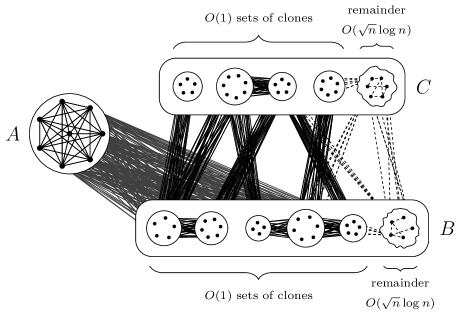
Figure 6: The partition $\{A,B,C\}$

In the third stage we show that the number of edges (and non-triangular edges) in $G$ is close to the number of edges (and non-triangular edges) in $G(|A|,|B|,|C|)$.

Proposition 30.

Let $A,B,C$ be as in Proposition 29 and denote $a=|A|,b=|B|,c=|C|$. Then $e(G)=a^{2}/2+ab+bc+O(ֿn^{7/4}\mathchoice{{\hbox{$\displaystyle\sqrt{\log n\,}$}\lower 0.4pt\hbox{\vrule height=6.94444pt,depth=-5.55559pt}}}{{\hbox{$\textstyle\sqrt{\log n\,}$}\lower 0.4pt\hbox{\vrule height=6.94444pt,depth=-5.55559pt}}}{{\hbox{$\scriptstyle\sqrt{\log n\,}$}\lower 0.4pt\hbox{\vrule height=4.8611pt,depth=-3.8889pt}}}{{\hbox{$\scriptscriptstyle\sqrt{\log n\,}$}\lower 0.4pt\hbox{\vrule height=3.47221pt,depth=-2.77779pt}}})$ and $t(G)=bc+O(n^{7/4}\mathchoice{{\hbox{$\displaystyle\sqrt{\log n\,}$}\lower 0.4pt\hbox{\vrule height=6.94444pt,depth=-5.55559pt}}}{{\hbox{$\textstyle\sqrt{\log n\,}$}\lower 0.4pt\hbox{\vrule height=6.94444pt,depth=-5.55559pt}}}{{\hbox{$\scriptstyle\sqrt{\log n\,}$}\lower 0.4pt\hbox{\vrule height=4.8611pt,depth=-3.8889pt}}}{{\hbox{$\scriptscriptstyle\sqrt{\log n\,}$}\lower 0.4pt\hbox{\vrule height=3.47221pt,depth=-2.77779pt}}})$.

In the final fourth stage we complete the proof of Theorem 5.

Proposition 31.

$G\cong G(a,b,c)$ for some $a,b,c$.

• The proof is immediate from Propositions 28, 29, 30 and 31. The only slight technicality is that when we replace a graph with at most $(1/2-\delta)n^{2}$ edges by an optimal and compressed graph, the number of edges may increase and exceed this bound. However, Lemma 13 implies that the number of edges can increase by at most $O(n)$, so the condition is still satisfied for a relaxed value of $\delta$. ∎

We now turn to the proofs of Propositions 28, 29, 30 and 31. We present them in separate subsections.

5.1 Many triangular vertices

In this subsection we prove Proposition 28.

See 28

The main ingredient of this proof is a surprising application of the exchange lemma, Lemma 13, and the assumption that $G$ is compressed. First, we conclude from Lemma 10 that $G$ has a large clique. Then, we partition the graph into fairly large independent sets of clones and a very dense part, using the fact that $G$ is compressed. It is then possible to conclude that only few of the vertices of the clique are adjacent to non-triangular edges.

• Our first aim is to show that $G$ has a clique of size at least $\Omega(n)$. This can be done fairly easily, as shown in the proof of the following claim.

  Claim 32.

  $G$ has a clique of size $\Omega(n)$.

• By Lemma 10, there exists a good weighted subgraph $H$ of $G$ satisfying $|H|=|G|=n$, $e(H)\geq e(G)$, $t(H)\geq t(G)$ (see Definition 9 for the definition of a good weighted graph). Let $\{K,\{u,v\}\}$ be a partition of $V(H)$ into a clique $K$ and an edge $uv$, which is the only non-triangular edge in $H$.

  Let $\alpha$ be the sum of the weights of the vertices in $K$ and let $m$ be the number of vertices in $K$. Let $\beta$ and $\gamma$ be the weights of $u$ and $v$ and suppose that $\beta\geq\gamma$. Note that $\alpha+\beta+\gamma=n$. By the Cauchy-Schwarz inequality, the contribution of the vertices in $K$ towards $e(H)$ is maximised if all of these vertices have weight $\alpha/m$. Therefore this contribution does not exceed $(\alpha/m)^{2}\binom{m}{2}=(1-1/m)\alpha^{2}/2$. Moreover, since no vertex is adjacent to both $u$ and $v$, the contribution of the edges between $K$ and $\{u,v\}$ towards $e(H)$ is maximised when every vertex in $K$ is adjacent to $u$, but not $v$. Hence,

  $$e(G)\leq e(H)\leq\left(1-\frac{1}{m}\right)\frac{\alpha^{2}}{2}+\alpha\beta+\beta\gamma.$$ (9)

  In particular, since $\beta\gamma\leq n^{2}/4$, we have $e(G)\leq n^{2}/4+\alpha n$. Recall that $e(G)\geq(1/4+\delta)n^{2}$. It follows that $\alpha\geq\delta n$.

  Denote $b=\lceil\beta\rceil$, $c=\lceil\gamma\rceil$ and $a=n-b-c$ and consider the graph $F=G(a,b,c)$. Note that $t(G)\leq t(H)=\beta\gamma\leq bc=t(F)$. Since $G$ is optimal, it follows that $e(G)\geq e(F)$. Therefore,

  $$e(G)\geq e(F) =\binom{a}{2}+ab+bc$$

  $$\geq\frac{(\alpha-2)(\alpha-3)}{2}+(\alpha-2)\beta+\beta\gamma$$

  $$\geq\frac{\alpha^{2}}{2}+\alpha\beta+\beta\gamma-2.5n$$

  $$=\left(1-\frac{5n}{\alpha^{2}}\right)\frac{\alpha^{2}}{2}+\alpha\beta+\beta\gamma.$$

  By (9) we have $m\geq\frac{\alpha^{2}}{5n}\geq\frac{\delta^{2}}{5}n$. It follows that $G$ has a clique of size at least $\frac{\delta^{2}}{5}n$. ∎

Recall that $G$ is compressed. It follows from Definition 14 that every independent set in $G$ of size at least $5n^{1/2}$ contains a set of clones of size at least $n^{1/2}$ (see Observation 15).

We construct a set $U\subseteq V(G)$ as follows. We start with $U=\emptyset$. At each stage, if the complement $U^{\mathsf{c}}=V(G)\setminus U$ contains an independent set $I$ of size at least $5n^{1/2}$, then $I$ contains a set of clones of size at least $n^{1/2}$. We add this set of clones to $U$ and continue until $U^{\mathsf{c}}$ has no independent set of size at least $5n^{1/2}$. Observe that $U$ is a disjoint union of sets of clones each of size at least $n^{1/2}$, while the complement $U^{\mathsf{c}}$ has no independent set of size at least $5n^{1/2}$ (see Figure 7).

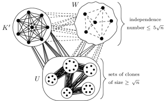
Figure 7: The sets $U$, $W$ and $K^{\prime}$

In the following claim we deduce from Lemma 13 that $G[U^{\mathsf{c}}]$ is very dense.

Claim 33.

$G[U^{\mathsf{c}}]$ has $O(n^{3/2})$ non-edges.

• Since $G[U^{\mathsf{c}}]$ has no independent set of size at least $5n^{1/2}$, every vertex in $G$ has at most $5n^{1/2}$ non-triangular neighbours in $U^{\mathsf{c}}$. It follows that the number of non-triangular edges with at least one end in $U^{\mathsf{c}}$ is at most $5n^{3/2}$.

  Denote by $m$ the number of non-edges in $G[U^{\mathsf{c}}]$. By adding these edges to $G$ we obtain a graph $G^{\prime}$ with $n$ vertices and $e(G)+m$ edges such that $t(G^{\prime})\geq t(G)-5n^{3/2}$. It follows from Lemma 13 that $m=O(n^{3/2})$. ∎

Let $K$ be a largest clique in $G$, so $|K|=\Omega(n)$ by Claim 32. Let $K^{\prime}=K\setminus U$ and denote $W=U^{\mathsf{c}}\setminus K^{\prime}$ (see Figure 7). Note that, since $U$ contains no clique of size greater than $n^{1/2}$, we have $|K^{\prime}|\geq|K|-n^{1/2}=\Omega(n)$. In the following claim we use the structure of $U$ and the previous claim to deduce that almost all the vertices in $K^{\prime}$ are triangular, i.e. are incident with triangular edges only.

Claim 34.

All but $O(n^{1/2})$ vertices in $K^{\prime}$ are triangular.

• Since $K^{\prime}$ is a clique, any vertex in the complement $V(G)\setminus K^{\prime}$ sends at most one non-triangular edge to $K^{\prime}$. In fact, if $u\in V(G)\setminus K^{\prime}$ has a non-triangular neighbour $v\in K^{\prime}$ then $u$ has no neighbours in $K^{\prime}$ except for $v$.

  Denote by $m$ the number of vertices in $W$ that have a non-triangular neighbour in $K^{\prime}$. Then the number of missing edges in $G[U^{\mathsf{c}}]$ is at least $m(|K^{\prime}|-1)=\Omega(mn)$. From Claim 33 we conclude that $m=O(n^{1/2})$. This implies that the number of vertices in $K^{\prime}$ that have a non-triangular neighbour in $U^{\mathsf{c}}$ is at most $O(n^{1/2})$.

  Finally, $U$ is a union of at most $n^{1/2}$ sets of clones, and any one set of clones can send non-triangular edges to at most one vertex in $K^{\prime}$. Therefore there are at most $n^{1/2}$ vertices in $K^{\prime}$ with a non-triangular neighbour in $U$. ∎

The clique $K^{\prime}$ is of size $\Omega(n)$ and we now know that all but $O(n^{1/2})$ vertices in $K^{\prime}$ are triangular. It follows that $G$ has $\Omega(n)$ triangular, completing the proof of Proposition 28. ∎

5.2 Structure

In this subsection we build on the fact that $G$ has $\Omega(n)$ triangular vertices and prove that, in terms of structure, $G$ is not far off from being isomorphic to a graph $G(a,b,c)$. In particular, we prove that the vertices of $G$ can be partitioned into three linearly sized sets $A,B,C$ such that $A$ is a clique, and all edges between $A$ and $B$ are present in $G$, while all edges between $A$ and $C$ are missing. We do not yet prove that the sets $B,C$ are independent, but we show that both of them can be partitioned into a small number of independent sets (see Figure 6). Our main tool in this subsection is the assumption that $G$ is compressed, we also use Lemma 13.

See 29

• Denote by $A$ the set of triangular vertices in $G$. Recall that $G$ is compressed, hence by Definition 14, the vertices of $A$ have the same neighbourhood outside of $A$. Denote this neighbourhood by $B$ and let $C=V(G)\setminus(A\cup B)$. Condition 1 follows.

  Note that the graph $G(a,b,c)$, where $c=\frac{\delta}{2}n$, $b=\mathchoice{{\hbox{$\displaystyle\sqrt{\delta\,}$}\lower 0.4pt\hbox{\vrule height=6.94444pt,depth=-5.55559pt}}}{{\hbox{$\textstyle\sqrt{\delta\,}$}\lower 0.4pt\hbox{\vrule height=6.94444pt,depth=-5.55559pt}}}{{\hbox{$\scriptstyle\sqrt{\delta\,}$}\lower 0.4pt\hbox{\vrule height=4.8611pt,depth=-3.8889pt}}}{{\hbox{$\scriptscriptstyle\sqrt{\delta\,}$}\lower 0.4pt\hbox{\vrule height=3.47221pt,depth=-2.77779pt}}}n$ and $a=n-b-c$, has at least $(1/2-\delta)n^{2}$ edges and $\frac{\delta^{3/2}}{2}n^{2}$ non-triangular edges. Hence, since $G$ is optimal and $e(G)\leq(1/2-\delta)n^{2}$, it follows that $t(G)=\Omega(n^{2})$.

  By Proposition 28 we have $|A|=\Omega(n)$. Note that there are no non-triangular edges with both ends in $B$, so the number of non-triangular edges in $G$ is at most $|C|(|B|+|C|)$. Since $t(G)=\Omega(n^{2})$, it follows that $|C|=\Omega(n)$. We will deduce that $|B|=\Omega(n)$ from a stronger statement that almost all vertices in $C$ have $\Omega(n)$ non-triangular neighbours in $B$.

  Claim 35.

  All but $O(1)$ vertices of $C$ have $\Omega(n)$ non-triangular neighbours in $B$.

• Let $c>0$ and $k\in\mathbb{N}$ be constants. Suppose that there is a set $Z\subseteq C$ of size $k$ whose every vertex has at most $cn$ non-triangular neighbours in $B$. Our aim is to show that if $c$ is sufficiently small and $k$ is sufficiently large, then no such set $Z$ exists.

  Consider the graph $G^{\prime}$, obtained from $G$ by adding the edges between $Z$ and $A$. Then $e(G^{\prime})=e(G)+k|A|$ and $t(G^{\prime})\geq t(G)-ckn-\binom{k}{2}\geq t(G)-2ckn$. Provided that $k$ is sufficiently large, Lemma 13 implies that $t(G^{\prime})\leq t(G)-\zeta k|A|$ for some constant $\zeta>0$ that does not depend on $c$ or $k$. Therefore $\zeta|A|\leq 2cn$ must hold. However, we may choose $c$ small enough to make this false, thus obtaining a contradiction. ∎

Denote by $C^{\prime}$ the set of vertices in $C$ that have $\Omega(n)$ neighbours in $B$. The previous claim implies that $|C\setminus C^{\prime}|=O(1)$. The following claim implies that $C^{\prime}$ may be partitioned into $O(1)$ independent sets.

Claim 36.

There exists a set $S\subseteq B$ of size $O(1)$ such that every vertex in $C^{\prime}$ has a non-triangular neighbour in $S$.

• We construct $S=\{u_{1},\dotsc,u_{k}\}$ by selecting the elements $u_{1},\dotsc,u_{k}\in B$ and subsets $I_{1},\ldots,I_{k}\subseteq B$ in the following way. Suppose that $u_{1},\ldots,u_{j}$ and $I_{1},\ldots,I_{j}$ have been selected, where $j\geq 0$. Consider the set $U_{j}$ consisting of vertices in $C^{\prime}$ that have a non-triangular neighbour in $\{u_{1},\ldots,u_{j}\}$ (so in particular $U_{0}=\emptyset$). If $U_{j}=C^{\prime}$, we stop the process. Otherwise, pick a vertex $v\in C^{\prime}\setminus U_{j}$ and consider the set $N$ consisting of the non-triangular neighbours of $v$ in $B$. By the definition of $C^{\prime}$, we have $|N|=\Omega(n)$. Moreover, since $N$ is independent and $G$ is compressed, $N$ contains a set of clones of size at least $|N|/5$. Denote this set of clones by $I_{j+1}$ and pick $u_{j+1}\in I_{j+1}$ arbitrarily.

  It is clear that when the process terminates, every vertex in $C^{\prime}$ has a non-triangular neighbour in the resulting set $S$. It remains to check that the process stops after $O(1)$ steps. Indeed, suppose that it ran for $k$ steps. The sets $I_{1},\ldots,I_{k}$ are pairwise disjoint and have size at least $\Omega(n)$ each, whence $k=O(1)$. ∎

The non-triangular neighbourhoods of the vertices in $S$ cover $C^{\prime}$. Therefore $C^{\prime}$ can be partitioned into $O(1)$ independent sets. Since $G$ is compressed, each independent set can be partitioned into $O(\log n)$ sets of clones, all but at most four of which have size $O(n^{1/3})$. Therefore $C^{\prime}$ can be partitioned into $O(1)$ sets of clones and a remainder of size $O(n^{1/3}\log n)$ (the $O(1)$ sets of clones being the four largest sets of clones within each independent set in the decomposition of $C^{\prime}$, and the remainder consisting of the remaining $O(\log n)$ sets of clones, each of which has size at most $O(n^{1/3})$). Note that, by definition, every vertex in $C^{\prime}$ has $\Omega(n)$ non-triangular neighbours in $B$. Now throw all of the $O(1)$ vertices of $C\setminus C^{\prime}$ into the remainder to get a partition of $C$ that satisfies Condition 3.

It remains to prove Condition 2. Let $Z$ denote the remainder in the partition of $C$ and denote $C^{\prime\prime}=C\setminus Z$. Let $Y$ be the set of vertices in $B$ that do not have non-triangular neighbours in $C^{\prime\prime}$ and denote $B^{\prime}=B\setminus Y$. We will show that $|Y|=O(n^{1/2}\log n)$ and that $B^{\prime}$ can be partitioned into $O(1)$ independent sets (from which it follows as before that $B^{\prime}$ can be partitioned into $O(1)$ sets of clones and a remainder of size $O(n^{1/3}\log n)$).

Claim 37.

$|Y|=O(n^{1/2}\log n)$.

• Recall that $A$ is the set of triangular vertices in $G$. Therefore every vertex in $B$ has a non-triangular neighbour, and that neighbour must be in $C$. In particular, the non-triangular neighbourhoods of $Z$ cover $Y$. Since $Z$ is a union of $O(\log n)$ sets of clones, this implies that $Y$ can be partitioned into $O(\log n)$ independent sets. In particular, $Y$ contains an independent set $I$ of size $\Omega(|Y|/\log n)$.

  Let $G^{\prime}$ be the graph obtained from $G$ by adding all possible edges spanned by $|I|$. Then $e(G^{\prime})=e(G)+\binom{|I|}{2}$ and $t(G^{\prime})\geq t(G)-|I||Z|\geq t(G)-O(|I|n^{1/3}\log n)$. This is a contradiction to Lemma 13 unless $\binom{|I|}{2}=O(n)$ or $\binom{|I|}{2}=O(|I|n^{1/3}\log n)$. In either case $|I|=O(n^{1/2})$ and so $|Y|=O(n^{1/2}\log n)$. ∎

To complete the proof of Proposition 29, it remains to show that $B^{\prime}$ can be partitioned into $O(1)$ independent sets. This is immediate upon recalling that $C^{\prime\prime}$ is the union of $O(1)$ sets of clones and that every vertex of $B^{\prime}$ has a non-triangular neighbour in $C^{\prime\prime}$. Indeed, $B^{\prime}$ is the union of the non-triangular neighbourhoods of the vertices in $C^{\prime\prime}$, and we have $O(1)$ such neighbourhoods. ∎

5.3 Sizes

In the previous subsection we proved that $V(G)$ can be partitioned into sets $A,B,C$ that correspond to the three parts of a graph $G(|A|,|B|,|C|)$. In this subsection we consider the sizes of the sets $A,B,C$. We show that the number of edges (and non-triangular edges) of $G$ is very close to the number of edges (and non-triangular edges) of $G(|A|,|B|,|C|)$.

See 30

In the proof of this proposition we revisit Füredi and Maleki’s proof [4] of Theorem 2 which is an approximate version of our main theorem. We simulate their proof of Lemma 10, but keep tight control on the order of vertices to which we apply Lemma 11.

• Recall that by Proposition 29 each of the sets $B$ and $C$ can be partitioned into $O(1)$ sets of clones and a remainder of size $O(n^{1/2}\log n)$. Let $G^{\prime}$ be the graph obtained by removing the edges adjacent to vertices in these remainders. Then $e(G^{\prime})\geq e(G)-O(n^{3/2}\log n)$ and $t(G^{\prime})\geq t(G)-O(n^{3/2}\log n)$.

  The following claim is a variation of Lemma 10. It allows us to approximate $G^{\prime}$ by a weighted graph that induces a clique on $C$.

  Claim 38.

  There is a weighted subgraph $H$ of $G^{\prime}$ such that $|H|=n$, $e(H)\geq e(G^{\prime})$ and $t(H)\geq t(G^{\prime})$. Furthermore, $H$ has the following properties.

  • All vertices in $A$ that are present in $H$, with at most one exception, have weight $1$.

  • All vertices in $B$ are present in $H$ and have weight $1$.

  • The vertices in $C$ that are present in $H$ induce a clique.

• We perform the following process to obtain the weighted graph $H$. Initially, we set $H$ to be $G^{\prime}$ with every vertex being given weight $1$. Then we perform multiple steps, during which we modify the weights of the vertices in $A\cup C$ (and remove some of these vertices) so that at any given time $A$ has at most one vertex with weight other than $1$. At each step we select vertices $u\in A$ and $v,w\in C$. We take $u$ to be the unique vertex in $A$ of weight not equal to $1$, and if there is no such vertex, we take it to be an arbitrary vertex remaining in $A$. We take $v$ and $w$ to be any pair of non-adjacent (in $G^{\prime}$) vertices in $C$. If choosing $u,v,w$ according to these rules is impossible, then we terminate the process.

  Suppose that we successfully selected the vertices $u,v,w$. We may remove one or two of them and redistribute their weight onto the remaining ones according to Lemma 11 so that the new weights are still positive, the total weight does not change and neither $e(H)$ nor $t(H)$ decrease. It is clear that this process terminates, because each step decreases the number of vertices remaining in $H$.

  Let us consider the resulting weighted graph $H$. Since the process terminated, either no vertices of $A$ are present in $H$, or the remaining vertices of $C$ induce a clique. We show that the latter condition must hold.

  Suppose that all vertices of $A$ were removed from $H$. Denote by $m$ the size of the largest clique that can be formed from vertices remaining in $H$. Since the vertex set of $G^{\prime}$ can be partitioned into $A$ and $O(1)$ independent sets, we have $m=O(1)$. Apply Lemma 10 to obtain a good weighted subgraph $F$ of $H$, with $xy$ being its only non-triangular edge, such that $|F|=n$, $e(F)\geq e(G^{\prime})$ and $t(F)\geq t(G^{\prime})$. Let $\beta$ and $\gamma$ be the weights of $x$ and $y$ in $F$ and suppose that $\beta\geq\gamma$. Then $\alpha=n-\beta-\gamma$ is the sum of the weights of the other vertices in $F$. We have $t(F)=\beta\gamma$ and, as in Inequality (9) from Claim 32, $e(F)\leq(1-1/m)\alpha^{2}/2+\alpha\beta+\beta\gamma$. It follows that $t(G)\leq\beta\gamma+O(n^{3/2}\log n)$ and $e(G)\leq\alpha^{2}/2+\alpha\beta+\beta\gamma-\Omega(n^{2})$. Consider the graph $G^{\prime\prime}=G(n-\lceil\beta\rceil-\lceil\gamma\rceil,\lceil\beta\rceil,\lceil\gamma\rceil)$. It is easy to check that $t(G^{\prime\prime})\geq t(G)-O(n^{3/2}\log n)$ and $e(G^{\prime\prime})\geq e(G)+\Omega(n^{2})$. This is a contradiction to Lemma 13, since $G$ is optimal.

  It follows that the set of vertices in $C$ that are present in $H$ induces a clique. Hence, the weighted graph $H$ satisfies the requirements of Claim 38. ∎

Let $H$ be a weighted graph as given by Claim 38, so in particular, $e(H)\geq e(G)-O(n^{3/2}\log n)$ and $t(H)\geq t(G)+O(n^{3/2}\log n)$. By Lemma 13, since $G$ is optimal,

$$\begin{split}e(H)&=e(G)+O\big{(}n^{3/2}\log n\big{)},\\ t(H)&=t(G)+O\big{(}n^{3/2}\log n\big{)}.\end{split}$$ (10)

We remark that these two lines express both upper and lower bounds for the quantities $e(H)$ and $t(H)$. In the following claim we prove that, in fact, only one vertex of $C$ is present in $H$.

Claim 39.

Exactly one vertex of $C$ is present in $H$. Moreover, all but at most $O(n^{3/4}\mathchoice{{\hbox{$\displaystyle\sqrt{\log n\,}$}\lower 0.4pt\hbox{\vrule height=6.94444pt,depth=-5.55559pt}}}{{\hbox{$\textstyle\sqrt{\log n\,}$}\lower 0.4pt\hbox{\vrule height=6.94444pt,depth=-5.55559pt}}}{{\hbox{$\scriptstyle\sqrt{\log n\,}$}\lower 0.4pt\hbox{\vrule height=4.8611pt,depth=-3.8889pt}}}{{\hbox{$\scriptscriptstyle\sqrt{\log n\,}$}\lower 0.4pt\hbox{\vrule height=3.47221pt,depth=-2.77779pt}}})$ vertices of $B$ are non-triangular neighbours of that vertex.

• Denote by $u_{1},\ldots,u_{m}$ the vertices in $C$ that are present in $H$, and let $N_{1},\dotsc,N_{m}$ be their non-triangular neighbourhoods in $B$. Since the set $\{u_{1},\dotsc,u_{m}\}$ forms a clique, there are no edges between $u_{i}$ and $N_{j}$ for $i\neq j$. In particular, the sets $N_{1},\dotsc,N_{m}$ are pairwise disjoint.

  Let $Z$ be the set of vertices in $B$ that have no non-triangular neighbours in $H$, that is, $Z=B\setminus(N_{1}\cup\ldots\cup N_{m})$. We will show that $|Z|=O(n^{3/4}\mathchoice{{\hbox{$\displaystyle\sqrt{\log n\,}$}\lower 0.4pt\hbox{\vrule height=6.94444pt,depth=-5.55559pt}}}{{\hbox{$\textstyle\sqrt{\log n\,}$}\lower 0.4pt\hbox{\vrule height=6.94444pt,depth=-5.55559pt}}}{{\hbox{$\scriptstyle\sqrt{\log n\,}$}\lower 0.4pt\hbox{\vrule height=4.8611pt,depth=-3.8889pt}}}{{\hbox{$\scriptscriptstyle\sqrt{\log n\,}$}\lower 0.4pt\hbox{\vrule height=3.47221pt,depth=-2.77779pt}}})$. Indeed, recall that $B$ is the union of $O(1)$ independent sets and a remainder of size at most $O(n^{1/2}\log n)$. Thus if $|Z|\geq\Omega(n^{3/4}\mathchoice{{\hbox{$\displaystyle\sqrt{\log n\,}$}\lower 0.4pt\hbox{\vrule height=6.94444pt,depth=-5.55559pt}}}{{\hbox{$\textstyle\sqrt{\log n\,}$}\lower 0.4pt\hbox{\vrule height=6.94444pt,depth=-5.55559pt}}}{{\hbox{$\scriptstyle\sqrt{\log n\,}$}\lower 0.4pt\hbox{\vrule height=4.8611pt,depth=-3.8889pt}}}{{\hbox{$\scriptscriptstyle\sqrt{\log n\,}$}\lower 0.4pt\hbox{\vrule height=3.47221pt,depth=-2.77779pt}}})$, there is an independent set $I\subseteq Z$ of size $\Omega(|Z|)$. Consider the weighted graph $H^{\prime}$ obtained from $H$ by adding the edges spanned by $I$. Then $e(H^{\prime})=e(H)+\Omega(|Z|^{2})\geq e(G)-O(n^{3/2}\log n)+\Omega(|Z|^{2})$ and $t(H^{\prime})=t(H)\geq t(G)-O(n^{3/2}\log n)$. It follows from Lemma 13 that $|Z|=O(n^{3/4}\mathchoice{{\hbox{$\displaystyle\sqrt{\log n\,}$}\lower 0.4pt\hbox{\vrule height=6.94444pt,depth=-5.55559pt}}}{{\hbox{$\textstyle\sqrt{\log n\,}$}\lower 0.4pt\hbox{\vrule height=6.94444pt,depth=-5.55559pt}}}{{\hbox{$\scriptstyle\sqrt{\log n\,}$}\lower 0.4pt\hbox{\vrule height=4.8611pt,depth=-3.8889pt}}}{{\hbox{$\scriptscriptstyle\sqrt{\log n\,}$}\lower 0.4pt\hbox{\vrule height=3.47221pt,depth=-2.77779pt}}})$.

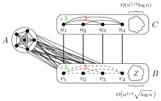
Figure 8: The graph $H^{\prime}$

Our aim is to prove that $m=1$. We assume for contradiction that $m\geq 2$. In particular, since in $G^{\prime}$ every vertex in $C$ is either isolated or has $\Omega(n)$ non-triangular neighbours in $B$, the vertices $u_{1},\dotsc,u_{m}$ have the latter property. In other words, $|N_{i}|=\Omega(n)$ for every $i$.

For each $i$, let $\gamma_{i}$ denote the weight of $u_{i}$ in $H$. We will show that $\gamma_{i}=\Omega(n)$ for every $i$. Indeed, fix any $i$. Denote by $H_{i}$ the weighted graph obtained from $H$ by adding all edges spanned by $N_{i}$. Since $N_{i}$ is an independent set in $H$, we have $e(H_{i})\geq e(G)+\Omega(n^{2})$ and $t(H_{i})\geq t(G)-|N_{i}|\gamma_{i}-O(n^{3/2}\log n)$. By Lemma 13, $\gamma_{i}=\Omega(n)$.

Write $\beta_{i}=|N_{i}|$. Construct a weighted graph $F$, starting from $H$ and carrying out the following steps. Firstly, remove all edges with an end in $Z$. Secondly, replace each set $N_{i}$ by a vertex $v_{i}$ of weight $\beta_{i}$. Finally, connect each vertex $v_{i}$ to all of the vertices in $A$ (that are present in $H$) as well as to $u_{i}$ and $v_{j}$ for every $j\neq i$. We have $e(F)\geq e(G)-O(n^{7/4}\mathchoice{{\hbox{$\displaystyle\sqrt{\log n\,}$}\lower 0.4pt\hbox{\vrule height=6.94444pt,depth=-5.55559pt}}}{{\hbox{$\textstyle\sqrt{\log n\,}$}\lower 0.4pt\hbox{\vrule height=6.94444pt,depth=-5.55559pt}}}{{\hbox{$\scriptstyle\sqrt{\log n\,}$}\lower 0.4pt\hbox{\vrule height=4.8611pt,depth=-3.8889pt}}}{{\hbox{$\scriptscriptstyle\sqrt{\log n\,}$}\lower 0.4pt\hbox{\vrule height=3.47221pt,depth=-2.77779pt}}})$ and $t(F)\geq t(H)\geq t(G)-O(n^{3/2}\log n)$.

Pick any real $\lambda$ such that $|\lambda|\leq\min\{\beta_{1},\beta_{2},\gamma_{1},\gamma_{2}\}$. Let $F_{\lambda}$ be the weighted graph obtained from $F$ by adding $\lambda$ to the weights of $u_{1}$ and $v_{1}$ and subtracting $\lambda$ from the weights of $u_{2}$ and $v_{2}$. Clearly, $|F_{\lambda}|=|F|=n$ and it is easy to check that $e(F_{\lambda})=e(F)$.

If $m\geq 3$, then the only non-triangular edges in $F$ are $u_{i}v_{i}$. Hence, in this case,

$$t(F_{\lambda}) =t(F)-(\beta_{1}\gamma_{1}+\beta_{2}\gamma_{2})+(\beta_{1}+\lambda)(\gamma_{1}+\lambda)+(\beta_{2}-\lambda)(\gamma_{2}-\lambda)$$

$$=t(F)+(\beta_{1}+\gamma_{1}-\beta_{2}-\gamma_{2})\lambda+2\lambda^{2}.$$

If $\beta_{1}+\gamma_{1}\geq\beta_{2}+\gamma_{2}$, then take $\lambda=\min\{\beta_{1},\gamma_{1},\beta_{2},\gamma_{2}\}$. Otherwise, take $\lambda=-\min\{\beta_{1},\gamma_{1},\beta_{2},\gamma_{2}\}$. In either case, $|\lambda|=\Omega(n)$ and $t(F_{\lambda})\geq t(F)+\Omega(n^{2})\geq t(G)+\Omega(n^{2})$, contradicting Lemma 13.

This calculation is slightly different in the case when $m=2$, because then we have to account for the edge $u_{1}u_{2}$, which is also non-triangular. In this case

$$t(F_{\lambda}) =t(F)-(\beta_{1}\gamma_{1}+\beta_{2}\gamma_{2}+\gamma_{1}\gamma_{2})+(\beta_{1}+\lambda)(\gamma_{1}+\lambda)+(\beta_{2}-\lambda)(\gamma_{2}-\lambda)+(\gamma_{1}+\lambda)(\gamma_{2}-\lambda)$$

$$=t(F)+(\beta_{1}-\beta_{2})\lambda+\lambda^{2}.$$

We may reach a contradiction to Lemma 13 by choosing $\gamma$ to be of the same sign as $\beta_{1}-\beta_{2}$ and $|\lambda|=\min\{\beta_{1},\beta_{2},\gamma_{1},\gamma_{2}\}$. We conclude that $m=1$, completing the proof of the claim. ∎

Recall that all but one vertex in $A$ has weight either $0$ or $1$ in $H$. In fact, we may assume that there are no vertices in $H$ with weight $0$. In the following claim we show that the remaining vertex cannot have very large weight.

Claim 40.

If some vertex in $A$ has weight (in $H$) other than $1$, then that weight is at most $O(n^{3/4}\mathchoice{{\hbox{$\displaystyle\sqrt{\log n\,}$}\lower 0.4pt\hbox{\vrule height=6.94444pt,depth=-5.55559pt}}}{{\hbox{$\textstyle\sqrt{\log n\,}$}\lower 0.4pt\hbox{\vrule height=6.94444pt,depth=-5.55559pt}}}{{\hbox{$\scriptstyle\sqrt{\log n\,}$}\lower 0.4pt\hbox{\vrule height=4.8611pt,depth=-3.8889pt}}}{{\hbox{$\scriptscriptstyle\sqrt{\log n\,}$}\lower 0.4pt\hbox{\vrule height=3.47221pt,depth=-2.77779pt}}})$.

• Let $u$ be a vertex of $A$ of maximal weight in $H$, and let $\omega$ be its weight. Suppose that $\omega>1$, in which case all other vertices in $A$ have weight $1$ in $H$.

  Replace the vertex $u$ by a clique of size $\lfloor\omega\rfloor$ whose vertices have weight $\omega/\lfloor\omega\rfloor$ and are adjacent to all of $(A\setminus\{u\})\cup B$ and denote the resulting weighted graph by $H^{\prime}$. We have to check the technical condition that the average weight of a vertex in $H^{\prime}$ is at least $1$. However, this can be easily verified, since the total weight of $H^{\prime}$ is an integer and $H^{\prime}$ has at most one vertex whose weight is smaller than $1$ (namely, the only vertex of $C$ that remains in $H^{\prime}$).

  We have $t(H^{\prime})=t(H)\geq t(G)-O(n^{3/2}\log n)$ and $e(H^{\prime})\geq e(G)-O(n^{3/2}\log n)+\Omega(\omega^{2})$. It follows from Lemma 13 that $\omega=O(n^{3/4}\mathchoice{{\hbox{$\displaystyle\sqrt{\log n\,}$}\lower 0.4pt\hbox{\vrule height=6.94444pt,depth=-5.55559pt}}}{{\hbox{$\textstyle\sqrt{\log n\,}$}\lower 0.4pt\hbox{\vrule height=6.94444pt,depth=-5.55559pt}}}{{\hbox{$\scriptstyle\sqrt{\log n\,}$}\lower 0.4pt\hbox{\vrule height=4.8611pt,depth=-3.8889pt}}}{{\hbox{$\scriptscriptstyle\sqrt{\log n\,}$}\lower 0.4pt\hbox{\vrule height=3.47221pt,depth=-2.77779pt}}})$. ∎

Recall that $a,b,c$ are the sizes of the sets $A,B,C$ in the original graph $G$. Let $\alpha,\beta,\gamma$ be the sums of weights (in $H$) of the vertices in these sets, summing over the vertices that are present in $H$. So, for example, $\beta=b$ and $\gamma$ is the weight of the single vertex in $C$ that is present in $H$. Clearly, $\alpha+\gamma=a+c$, because both sides are equal to $n-b$. Now we use the properties of $H$ that we have proved to get good bounds on $e(H)$ and $t(H)$ in terms of $\alpha,\beta,\gamma$.

Recall that the set $A$ induces a clique in $G$, so its remainder induces a clique in $H$. Combined with Claim 40, this implies that the contribution of the edges within $A$ to $e(H)$ is $\alpha^{2}/2-O(n^{3/2}\log n)$. By Claim 39, the set $B$ contains an independent set of size at least $|B|-O(n^{3/4}\mathchoice{{\hbox{$\displaystyle\sqrt{\log n\,}$}\lower 0.4pt\hbox{\vrule height=6.94444pt,depth=-5.55559pt}}}{{\hbox{$\textstyle\sqrt{\log n\,}$}\lower 0.4pt\hbox{\vrule height=6.94444pt,depth=-5.55559pt}}}{{\hbox{$\scriptstyle\sqrt{\log n\,}$}\lower 0.4pt\hbox{\vrule height=4.8611pt,depth=-3.8889pt}}}{{\hbox{$\scriptscriptstyle\sqrt{\log n\,}$}\lower 0.4pt\hbox{\vrule height=3.47221pt,depth=-2.77779pt}}})$. Therefore the contribution of the edges within $B$ to $e(H)$ (and in particular to $t(H)$) is $O(n^{7/4}\mathchoice{{\hbox{$\displaystyle\sqrt{\log n\,}$}\lower 0.4pt\hbox{\vrule height=6.94444pt,depth=-5.55559pt}}}{{\hbox{$\textstyle\sqrt{\log n\,}$}\lower 0.4pt\hbox{\vrule height=6.94444pt,depth=-5.55559pt}}}{{\hbox{$\scriptstyle\sqrt{\log n\,}$}\lower 0.4pt\hbox{\vrule height=4.8611pt,depth=-3.8889pt}}}{{\hbox{$\scriptscriptstyle\sqrt{\log n\,}$}\lower 0.4pt\hbox{\vrule height=3.47221pt,depth=-2.77779pt}}})$. Moreover, Claim 39 implies that the edges between $B$ and $C$ contribute $\beta\gamma-O(n^{7/4}\mathchoice{{\hbox{$\displaystyle\sqrt{\log n\,}$}\lower 0.4pt\hbox{\vrule height=6.94444pt,depth=-5.55559pt}}}{{\hbox{$\textstyle\sqrt{\log n\,}$}\lower 0.4pt\hbox{\vrule height=6.94444pt,depth=-5.55559pt}}}{{\hbox{$\scriptstyle\sqrt{\log n\,}$}\lower 0.4pt\hbox{\vrule height=4.8611pt,depth=-3.8889pt}}}{{\hbox{$\scriptscriptstyle\sqrt{\log n\,}$}\lower 0.4pt\hbox{\vrule height=3.47221pt,depth=-2.77779pt}}})$ to both $e(H)$ and $t(H)$. Putting this together, we get

$$\begin{split}e(H)&=\alpha^{2}/2+\alpha\beta+\beta\gamma+O\big{(}n^{7/4}\mathchoice{{\hbox{$\displaystyle\sqrt{\log n\,}$}\lower 0.4pt\hbox{\vrule height=6.94444pt,depth=-5.55559pt}}}{{\hbox{$\textstyle\sqrt{\log n\,}$}\lower 0.4pt\hbox{\vrule height=6.94444pt,depth=-5.55559pt}}}{{\hbox{$\scriptstyle\sqrt{\log n\,}$}\lower 0.4pt\hbox{\vrule height=4.8611pt,depth=-3.8889pt}}}{{\hbox{$\scriptscriptstyle\sqrt{\log n\,}$}\lower 0.4pt\hbox{\vrule height=3.47221pt,depth=-2.77779pt}}}\big{)}\\ t(H)&=\beta\gamma+O\big{(}n^{7/4}\mathchoice{{\hbox{$\displaystyle\sqrt{\log n\,}$}\lower 0.4pt\hbox{\vrule height=6.94444pt,depth=-5.55559pt}}}{{\hbox{$\textstyle\sqrt{\log n\,}$}\lower 0.4pt\hbox{\vrule height=6.94444pt,depth=-5.55559pt}}}{{\hbox{$\scriptstyle\sqrt{\log n\,}$}\lower 0.4pt\hbox{\vrule height=4.8611pt,depth=-3.8889pt}}}{{\hbox{$\scriptscriptstyle\sqrt{\log n\,}$}\lower 0.4pt\hbox{\vrule height=3.47221pt,depth=-2.77779pt}}}\big{)}.\end{split}$$ (11)

Again, we remark that these are both upper and lower bounds for the quantities $e(H)$ and $t(H)$. We deduce that $\alpha$ almost equals $a$ and $\gamma$ almost equals $c$.

Claim 41.

$\alpha=a+O(n^{3/4}\mathchoice{{\hbox{$\displaystyle\sqrt{\log n\,}$}\lower 0.4pt\hbox{\vrule height=6.94444pt,depth=-5.55559pt}}}{{\hbox{$\textstyle\sqrt{\log n\,}$}\lower 0.4pt\hbox{\vrule height=6.94444pt,depth=-5.55559pt}}}{{\hbox{$\scriptstyle\sqrt{\log n\,}$}\lower 0.4pt\hbox{\vrule height=4.8611pt,depth=-3.8889pt}}}{{\hbox{$\scriptscriptstyle\sqrt{\log n\,}$}\lower 0.4pt\hbox{\vrule height=3.47221pt,depth=-2.77779pt}}})$ and $\gamma=c+O(n^{3/4}\mathchoice{{\hbox{$\displaystyle\sqrt{\log n\,}$}\lower 0.4pt\hbox{\vrule height=6.94444pt,depth=-5.55559pt}}}{{\hbox{$\textstyle\sqrt{\log n\,}$}\lower 0.4pt\hbox{\vrule height=6.94444pt,depth=-5.55559pt}}}{{\hbox{$\scriptstyle\sqrt{\log n\,}$}\lower 0.4pt\hbox{\vrule height=4.8611pt,depth=-3.8889pt}}}{{\hbox{$\scriptscriptstyle\sqrt{\log n\,}$}\lower 0.4pt\hbox{\vrule height=3.47221pt,depth=-2.77779pt}}})$.

• We can read the inequality $\alpha\leq a+O(n^{3/4}\mathchoice{{\hbox{$\displaystyle\sqrt{\log n\,}$}\lower 0.4pt\hbox{\vrule height=6.94444pt,depth=-5.55559pt}}}{{\hbox{$\textstyle\sqrt{\log n\,}$}\lower 0.4pt\hbox{\vrule height=6.94444pt,depth=-5.55559pt}}}{{\hbox{$\scriptstyle\sqrt{\log n\,}$}\lower 0.4pt\hbox{\vrule height=4.8611pt,depth=-3.8889pt}}}{{\hbox{$\scriptscriptstyle\sqrt{\log n\,}$}\lower 0.4pt\hbox{\vrule height=3.47221pt,depth=-2.77779pt}}})$ off Claim 40. To get the upper bound on $\alpha$, we consider the quantity $e(H)-t(H)$. On one hand, the inequalities in (11) give

  $$e(H)-t(H)=\alpha^{2}/2+\alpha\beta+O\big{(}n^{7/4}\mathchoice{{\hbox{$\displaystyle\sqrt{\log n\,}$}\lower 0.4pt\hbox{\vrule height=6.94444pt,depth=-5.55559pt}}}{{\hbox{$\textstyle\sqrt{\log n\,}$}\lower 0.4pt\hbox{\vrule height=6.94444pt,depth=-5.55559pt}}}{{\hbox{$\scriptstyle\sqrt{\log n\,}$}\lower 0.4pt\hbox{\vrule height=4.8611pt,depth=-3.8889pt}}}{{\hbox{$\scriptscriptstyle\sqrt{\log n\,}$}\lower 0.4pt\hbox{\vrule height=3.47221pt,depth=-2.77779pt}}}\big{)}.$$

  On the other hand, we can use the inequalities in (10) to get

  $$e(H)-t(H) =e(G)-t(G)+O(n^{3/2}\log n)$$

  $$\geq a^{2}/2+ab+O(n^{3/2}\log n),$$

  where the latter inequality comes from the fact that the quantity $e(G)-t(G)$ counts the triangular edges in $G$, and all vertices in $A$ are triangular. Recall that $b=\beta$. Combining the two inequalities for $e(H)-t(H)$ we get $\alpha\geq a+O(n^{3/4}\mathchoice{{\hbox{$\displaystyle\sqrt{\log n\,}$}\lower 0.4pt\hbox{\vrule height=6.94444pt,depth=-5.55559pt}}}{{\hbox{$\textstyle\sqrt{\log n\,}$}\lower 0.4pt\hbox{\vrule height=6.94444pt,depth=-5.55559pt}}}{{\hbox{$\scriptstyle\sqrt{\log n\,}$}\lower 0.4pt\hbox{\vrule height=4.8611pt,depth=-3.8889pt}}}{{\hbox{$\scriptscriptstyle\sqrt{\log n\,}$}\lower 0.4pt\hbox{\vrule height=3.47221pt,depth=-2.77779pt}}})$, so $\alpha=a+O(n^{3/4}\mathchoice{{\hbox{$\displaystyle\sqrt{\log n\,}$}\lower 0.4pt\hbox{\vrule height=6.94444pt,depth=-5.55559pt}}}{{\hbox{$\textstyle\sqrt{\log n\,}$}\lower 0.4pt\hbox{\vrule height=6.94444pt,depth=-5.55559pt}}}{{\hbox{$\scriptstyle\sqrt{\log n\,}$}\lower 0.4pt\hbox{\vrule height=4.8611pt,depth=-3.8889pt}}}{{\hbox{$\scriptscriptstyle\sqrt{\log n\,}$}\lower 0.4pt\hbox{\vrule height=3.47221pt,depth=-2.77779pt}}})$. To complete the proof of the claim, note that $a+c=\alpha+\gamma$. ∎

Proposition 29 follows from the last claim and the inequalities in (11). ∎

5.4 End of the proof

We are now ready to complete the proof of Theorem 5.

See 31

We gradually get closer to proving that $G\cong G(a,b,c)$. We start by showing that $b$ is much bigger than $c$, which leads to the conclusion that $C$ spans no non-triangular edges. This implies that almost all possible edges between $B$ and $C$ are present in $G$ and are non-triangular, by Proposition 30. In fact, using the fact that $G$ is compressed, we deduce that there are large subsets of $B$ and of $C$ that span a complete bipartite graph consisting of non-triangular edges. With some more effort, using the optimality of $G$, we conclude that $B$ and $C$ themselves induce a complete bipartite graph, thus completing the proof.

• Let $\{A,B,C\}$ be the partition of $V(G)$ given by Proposition 29. As in the statement of Proposition 30, write $a=|A|,b=|B|,c=|C|$. We start by showing that $b$ is significantly larger than $c$.

  Claim 42.

  We have $b\geq c+\Omega(n)$.

• Suppose to the contrary that $b\leq c+o(n)$. Then we have $n=a+b+c\geq 2b+a-o(n)$, and hence $b\leq(n-a+o(n))/2$. Since $a=\Omega(n)$, we can conclude that $b\leq n/2-\Omega(n)$.

  Consider the graph $H=G(a,b,c)$. Proposition 30 implies that $e(H)=e(G)+O(n^{7/4}\mathchoice{{\hbox{$\displaystyle\sqrt{\log n\,}$}\lower 0.4pt\hbox{\vrule height=6.94444pt,depth=-5.55559pt}}}{{\hbox{$\textstyle\sqrt{\log n\,}$}\lower 0.4pt\hbox{\vrule height=6.94444pt,depth=-5.55559pt}}}{{\hbox{$\scriptstyle\sqrt{\log n\,}$}\lower 0.4pt\hbox{\vrule height=4.8611pt,depth=-3.8889pt}}}{{\hbox{$\scriptscriptstyle\sqrt{\log n\,}$}\lower 0.4pt\hbox{\vrule height=3.47221pt,depth=-2.77779pt}}})$ and $t(H)=t(G)+O(n^{7/4}\mathchoice{{\hbox{$\displaystyle\sqrt{\log n\,}$}\lower 0.4pt\hbox{\vrule height=6.94444pt,depth=-5.55559pt}}}{{\hbox{$\textstyle\sqrt{\log n\,}$}\lower 0.4pt\hbox{\vrule height=6.94444pt,depth=-5.55559pt}}}{{\hbox{$\scriptstyle\sqrt{\log n\,}$}\lower 0.4pt\hbox{\vrule height=4.8611pt,depth=-3.8889pt}}}{{\hbox{$\scriptscriptstyle\sqrt{\log n\,}$}\lower 0.4pt\hbox{\vrule height=3.47221pt,depth=-2.77779pt}}})$. Consider also the graph $H^{\prime}=G(a,b+d,c-d)$, where $d=\lfloor n^{1.999}\rfloor$. Note that $b+d\leq n/2-\Omega(n)$. Therefore, from the expression $e(H)=\binom{a}{2}+(n-b)b$ and the corresponding expression for $e(H^{\prime})$, we can see that $e(H^{\prime})\geq e(H)+\Omega(dn)=e(G)+\Omega(dn)$. Similarly, $t(H^{\prime})\geq t(H)-o(dn)=t(G)-o(dn)$. However, this contradicts Lemma 13, so $b=c+\Omega(n)$. ∎

In the following claim we conclude that $C$ spans no non-triangular edges.

Claim 43.

There are no non-triangular edges with both ends in $C$.

• By Proposition 30 there are $bc+o(n^{2})$ non-triangular edges in $G$, and each one of them is incident with a vertex in $C$. Therefore some vertex in $C$ has at least $b-o(n)$ non-triangular neighbours. Thus, by Observation 8, every vertex in $C$ has degree at least $b-o(n)$, so the sum of the degrees of any two vertices in $C$ is at least $2b-o(n)>b+c=|B\cup C|$, where the latter inequality comes from the previous claim. Since the vertices in $C$ have neighbours only in $B\cup C$, it follows that any pair of vertices in $C$ have a common neighbour, hence they cannot be joined by a non-triangular edge. ∎

Recall that by Proposition 29 each of the sets $B$ and $C$ can be partitioned into $O(1)$ sets of clones and a remainder of size $O(n^{1/2}\log n)$. In such a partition of $B$ consider the sets of clones of size at least $n^{9/10}$ and let $B^{\prime}$ be their union. Similarly, let $C^{\prime}$ be the union of the sets of clones in the partition of $C$ that have size at least $n^{9/10}$ and denote $Z=C\setminus C^{\prime}$ and $Y=B\setminus B^{\prime}$. Then $|Y|=O(n^{9/10})$ and $|Z|=O(n^{9/10})$. We show that all possible edges between $B^{\prime}$ and $C^{\prime}$ are present in $G$ and are non-triangular.

Claim 44.

All possible edges between $B^{\prime}$ and $C^{\prime}$ are present in $G$ and are non-triangular.

• From the previous claim we know that every non-triangular edge in $G$ has one end in $B$ and one end in $C$. Suppose that there is a pair of vertices, one in $B^{\prime}$ and one in $C^{\prime}$, that are not joined by a non-triangular edge. Then there are two sets of clones of size at least $n^{9/10}$, one contained in $B^{\prime}$ and the other in $C^{\prime}$, between which there are no non-triangular edges. But then $t(G)\leq bc-n^{9/5}$, contradicting Proposition 30. ∎

In the following claim we obtain additional information about $Y$ and $Z$, thereby we get close to showing that $B$ and $C$ induce a complete bipartite graph.

Claim 45.

There are no edges between $B^{\prime}$ and $Y$ and between $C^{\prime}$ and $Z$. Moreover, every vertex in $B$ has at least $c-o(n)$ neighbours in $C$, and every vertex in $C$ has at least $b-o(n)$ neighbours in $B$.

• Any vertex in $C^{\prime}$ has at least $|B^{\prime}|=b-o(n)$ non-triangular neighbours, so Observation 8 implies that every vertex in $G$ has degree at least $b-o(n)$. Claim 42 implies that $|C|+|B\setminus B^{\prime}|\leq c+o(n)$ is smaller than this quantity, hence every vertex in $C$ has a neighbour in $B^{\prime}$. Therefore, because all possible edges between $B^{\prime}$ and $C^{\prime}$ are present in $G$ and are non-triangular (by Claim 44), there are no edges between $C^{\prime}$ and $Z$. In particular, every vertex in $C$ has at most $o(n)$ neighbours in $C$, so it has at least $b-o(n)$ neighbours in $B$.

  Pick any vertex $u\in Y$. Since $u$ is not in $A$, $u$ has a non-triangular neighbour $v\in C$. We have just proved that $v$ has at least $b-o(n)$ neighbours in $B^{\prime}$. Therefore, $u$ has at most $o(n)$ neighbours in $B$. Now suppose that $u$ is adjacent to a vertex in $B^{\prime}$. Then $u$ has no neighbours in $C^{\prime}$. Hence, $u$ has at most $a+o(n)$ neighbours, of which at most $o(n)$ are non-triangular. However, any vertex of $B^{\prime}$ has at least $a+c-o(n)$ neighbours and at least $c-o(n)$ of them are non-triangular. This contradicts Observation 8.

  It remains to verify that every vertex in $Y$ has at least $c-o(n)$ neighbours in $C$. Let $w\in Y$ and denote by $d$ the number of neighbours of $w$ in $C$. Then the degree of $w$ is at most $a+d+o(n)$ and its non-triangular degree is at most $d$. By Observation 8, applied to $w$ and any vertex in $B^{\prime}$, we know that $a+d\geq a+c-o(n)$ or $d\geq c-o(n)$. In either case $d\geq c-o(n)$. ∎

In the following claim we prove that no edges are spanned by $Z$. We use a trick that we have used several times before, replacing a pair of adjacent vertices in $Z$ by copies of vertices in $A$ and $B^{\prime}$, thus increasing both the number of edges and of triangular edges.

Claim 46.

$Z$ spans no edges.

• Suppose to the contrary that $Z$ contains a pair of adjacent vertices $u,v$. All of the non-triangular neighbours of $u$ are in $B$ and they are not adjacent to $v$. By Claim 45, $v$ has $b-o(n)$ neighbours in $B$, and hence $u$ has at most $o(n)$ non-triangular neighbours. Likewise, $v$ has at most $o(n)$ non-triangular neighbours.

  Consider the graph $G^{\prime}$ obtained from $G$ by removing $u,v$ and adding new vertices $x$ and $y$, where $x$ is joined by edges to all vertices in $A\cup B$, and $y$ is joined to all vertices in $B^{\prime}$ (in other words, $u$ and $v$ are replaced by two new vertices, one in $A$ and one in $B^{\prime}$). We have $e(G^{\prime})\geq e(G)+a-o(n)$ and $t(G^{\prime})\geq t(G)+b-o(n)$. This contradicts the optimality of $G$, because $a=\Omega(n)$ and $b=\Omega(n)$. ∎

A similar trick enables us to conclude that $Y$ spans no edges, but here we replace all non-isolate vertices in $Y$ with suitable copies of other vertices.

Claim 47.

There are no edges with both ends in $Y$.

• Let $S$ be the set of vertices in $Y$ that have a neighbour in $Y$. Our aim is to prove that $S=\emptyset$. To this end, write $m=|S|$ and suppose that $m\neq 0$. Then $2\leq m=o(n)$. Let $G^{\prime}$ be the graph obtained from $G$ by removing all vertices in $S$, adding $\lfloor m/2\rfloor$ new vertices to $A$ and adding $\lceil m/2\rceil$ new vertices to $B^{\prime}$. More precisely, we add $\lfloor m/2\rfloor$ new vertices adjacent to all of $A\cup B^{\prime}$ and $\lceil m/2\rceil$ more new vertices adjacent to all of $A\cup C^{\prime}$.

  Let us compare $e(G^{\prime})$ and $t(G^{\prime})$ with $e(G)$ and $t(G)$. It follows from Claims 44 and 45 that if an edge in $G$ has both ends in $B$, then in fact it has both ends in $S$. In particular, the removal of $S$ decreases the total number of edges by at most $(a+c)m+\binom{m}{2}=(a+c+o(n))m$. On the other hand, the addition of the new vertices increases this number by $(a+c-o(n))m+(b-c)\lfloor m/2\rfloor\geq(a+c+\Omega(n))m$. Therefore, $e(G^{\prime})\geq e(G)+\Omega(mn)>e(G)$.

  Moreover, in $G$, every vertex in $S$ has at most $o(n)$ non-triangular neighbours, because every vertex in $S$ is adjacent to another vertex in $S$, which has at least $c-o(n)$ neighbours in $C$. Therefore, the removal of $S$ decreases the number of non-triangular edges by at most $o(mn)$. On the other hand, the addition of new vertices increases this number by $(b-o(n))\lceil m/2\rceil=\Omega(mn)$. Therefore, $t(G^{\prime})>t(G)$ and this contradicts the optimality of $G$. This means that $m=0$, so $Y$ spans no edges. ∎

Proposition 31 easily follows from Claims 44, 45, 46 and 47. Indeed, these claims together imply that $B$ and $C$ are independent sets in $G$. Therefore, if there were missing edges between $B$ and $C$, we could add them to $G$ without creating new triangles. Since $G$ is an optimal graph, all possible edges between $B$ and $C$ are present. It follows that $G\cong G(|A|,|B|,|C|)$. ∎

6 Almost complete

In this section we prove Theorem 6.

See 6

The proof in this range is easier than the other two ranges, though far from immediate. We start by proving that $G\cong G(a,b,c)$ for some $a,b,c$ if there are only very few (at most $2n-8$) missing edges. For the remaining range, we obtain a partition of the vertices into sets $A,B,C$ according to the degrees of the vertices and aim to show that $G\cong G(|A|,|B|,|C|)$. We first prove that the sets have the correct orders of magnitude using a rough lower bound on $t(G)$. We are then able to prove better estimates for the size of the sets, and, finally, we deduce that $G$ has the required structure.

Fix a small constant $\delta>0$ (whose value can be worked out from the proof) and let $G$ be an optimal graph with $n$ vertices and $\binom{n}{2}-\varepsilon n^{2}$ edges, where $0\leq\varepsilon\leq\delta$. We may assume that the set of triangular induces a clique and all its vertices have the same neighbourhood among the remaining vertices (see e.g. Lemma 16). As usually, we assume that $n$ is large enough to satisfy all inequalities that we write down in the proof.

We first consider the case $e(G)\geq\binom{n}{2}-(2n-9)$.

Claim 48.

If $e(G)\geq\binom{n}{2}-(2n-9)$ then $G\cong G(a,b,c)$ for some $a,b,c$.

• If $G$ has no non-triangular edges, then by optimality, it is a clique, so we are done ($G=G(n,0,0)$). We claim that $G$ does not have two independent non-triangular edges. Indeed, if $uv$ and $xy$ are such edges, then for any other vertex $w$ one of the two possible edges $uw$ and $vw$ is missing, as well as one of $xw$ and $yw$. Therefore $G$ has at least $2n-8$ missing edges, contradicting our assumption. Therefore, since the triangle-free edges cannot form a triangle, they form a star. Let $uv_{1},\dotsc,uv_{k}$ be the non-triangular edges. Then the set $A=V(G)\setminus\{u,v_{1},\dotsc,v_{k}\}$ is the set of triangular vertices in $G$, so $A$ induces a clique and all of the vertices in $A$ have the same neighbourhood in $V(G)\setminus A$. So there are two possibilities: either $u$ is adjacent to all of $A$, or $u$ is not adjacent to any vertex in $A$. In the former case, there are no edges between $A$ and $\{u_{1},\dotsc,u_{k}\}$, so $G\cong G(|A|,1,k)$. In the latter case, optimality of $G$ implies that all possible edges between $A$ and $\{u_{1},\dotsc,u_{k}\}$ are present in $G$, so $G\cong G(|A|,k,1)$. ∎

From this point onwards we assume that $e(G)\leq\binom{n}{2}-(2n-8)$. In particular, $\varepsilon\geq(2-o(1))/n$. We wish to prove that $G$ is isomorphic to the graph $G(a,b,c)$ for some parameters $a,b,c$. It is easy to see that these parameters should be approximately equal to $b\approx\mathchoice{{\hbox{$\displaystyle\sqrt{2\varepsilon/3\,}$}\lower 0.4pt\hbox{\vrule height=7.5pt,depth=-6.00003pt}}}{{\hbox{$\textstyle\sqrt{2\varepsilon/3\,}$}\lower 0.4pt\hbox{\vrule height=7.5pt,depth=-6.00003pt}}}{{\hbox{$\scriptstyle\sqrt{2\varepsilon/3\,}$}\lower 0.4pt\hbox{\vrule height=5.25pt,depth=-4.20003pt}}}{{\hbox{$\scriptscriptstyle\sqrt{2\varepsilon/3\,}$}\lower 0.4pt\hbox{\vrule height=3.75pt,depth=-3.00002pt}}}n$ and $c\approx(2\varepsilon/3)n$, because this is when $bc$ is maximised subject to conditions $n=a+b+c$ and $cn+\binom{b}{2}\leq\varepsilon n$. We use this observation to get a lower bound for $t(G)$.

Claim 49.

$t(G)=\Omega(\varepsilon^{3/2}n^{2})$.

• Let $G^{\prime}=G(a,b,c)$, where $b=\lfloor\mathchoice{{\hbox{$\displaystyle\sqrt{2\varepsilon/3\,}$}\lower 0.4pt\hbox{\vrule height=7.5pt,depth=-6.00003pt}}}{{\hbox{$\textstyle\sqrt{2\varepsilon/3\,}$}\lower 0.4pt\hbox{\vrule height=7.5pt,depth=-6.00003pt}}}{{\hbox{$\scriptstyle\sqrt{2\varepsilon/3\,}$}\lower 0.4pt\hbox{\vrule height=5.25pt,depth=-4.20003pt}}}{{\hbox{$\scriptscriptstyle\sqrt{2\varepsilon/3\,}$}\lower 0.4pt\hbox{\vrule height=3.75pt,depth=-3.00002pt}}}n\rfloor$, $c=\lfloor(2\varepsilon/3)n\rfloor$ and $a=n-b-c$. Then the number of edges missing from $G^{\prime}$ is at most $\binom{b}{2}+cn\leq\varepsilon n$. We now find a lower bound for $t(G^{\prime})$, but we need to be careful with the rounding-down errors in the definitions of $b$ and $c$.

  Recall that $\varepsilon n^{2}\geq 2n-9$, implying that $(2\varepsilon/3)n\geq 4/3-6/n$, hence $c=\lfloor(2\varepsilon/3)n\rfloor\geq\frac{1}{5}(2\varepsilon/3)n=(2\varepsilon/15)n$. Since $\varepsilon n^{2}\geq 2n-9$, we have $\mathchoice{{\hbox{$\displaystyle\sqrt{\varepsilon\,}$}\lower 0.4pt\hbox{\vrule height=4.30554pt,depth=-3.44446pt}}}{{\hbox{$\textstyle\sqrt{\varepsilon\,}$}\lower 0.4pt\hbox{\vrule height=4.30554pt,depth=-3.44446pt}}}{{\hbox{$\scriptstyle\sqrt{\varepsilon\,}$}\lower 0.4pt\hbox{\vrule height=3.01389pt,depth=-2.41113pt}}}{{\hbox{$\scriptscriptstyle\sqrt{\varepsilon\,}$}\lower 0.4pt\hbox{\vrule height=2.15277pt,depth=-1.72223pt}}}n\geq\mathchoice{{\hbox{$\displaystyle\sqrt{2n-9\,}$}\lower 0.4pt\hbox{\vrule height=6.44444pt,depth=-5.15558pt}}}{{\hbox{$\textstyle\sqrt{2n-9\,}$}\lower 0.4pt\hbox{\vrule height=6.44444pt,depth=-5.15558pt}}}{{\hbox{$\scriptstyle\sqrt{2n-9\,}$}\lower 0.4pt\hbox{\vrule height=4.51111pt,depth=-3.6089pt}}}{{\hbox{$\scriptscriptstyle\sqrt{2n-9\,}$}\lower 0.4pt\hbox{\vrule height=3.22221pt,depth=-2.57779pt}}}$, hence, very crudely, $b\geq(\mathchoice{{\hbox{$\displaystyle\sqrt{\varepsilon/3\,}$}\lower 0.4pt\hbox{\vrule height=7.5pt,depth=-6.00003pt}}}{{\hbox{$\textstyle\sqrt{\varepsilon/3\,}$}\lower 0.4pt\hbox{\vrule height=7.5pt,depth=-6.00003pt}}}{{\hbox{$\scriptstyle\sqrt{\varepsilon/3\,}$}\lower 0.4pt\hbox{\vrule height=5.25pt,depth=-4.20003pt}}}{{\hbox{$\scriptscriptstyle\sqrt{\varepsilon/3\,}$}\lower 0.4pt\hbox{\vrule height=3.75pt,depth=-3.00002pt}}})n$. It follows that $t(G^{\prime})=bc\geq\lambda\varepsilon^{3/2}n^{2}$, for $\lambda=2/(15\mathchoice{{\hbox{$\displaystyle\sqrt{3\,}$}\lower 0.4pt\hbox{\vrule height=6.44444pt,depth=-5.15558pt}}}{{\hbox{$\textstyle\sqrt{3\,}$}\lower 0.4pt\hbox{\vrule height=6.44444pt,depth=-5.15558pt}}}{{\hbox{$\scriptstyle\sqrt{3\,}$}\lower 0.4pt\hbox{\vrule height=4.51111pt,depth=-3.6089pt}}}{{\hbox{$\scriptscriptstyle\sqrt{3\,}$}\lower 0.4pt\hbox{\vrule height=3.22221pt,depth=-2.57779pt}}})$. Since $G$ is optimal, it follows that $t(G)\geq t(G^{\prime})=\Omega(\varepsilon^{3/2}n^{2})$. ∎

We now define three sets $A,B,C\subseteq V(G)$ that correspond to the three parts of a graph $G(a,b,c)$. Let $C$ be the set of vertices of degree at most $3n/4$; let $B$ be the set of vertices in $V(G)\setminus C$ that have a non-triangular neighbour in $C$; and let $A=V(G)\setminus(B\cup C)$. Since any two vertices in $A\cup B$ have at least $n/2$ common neighbours, there are no non-triangular edges in $A\cup B$. Therefore, all vertices in $A$ are triangular, so $A$ induces a clique and its vertices have the same neighbourhood in $V(G)\setminus A$.

The next step is to obtain tight bounds for the sizes of $A,B,C$. First, we determine the order of magnitude of $|B|$ and $|C|$.

Claim 50.

$|B|=\Theta(\mathchoice{{\hbox{$\displaystyle\sqrt{\varepsilon\,}$}\lower 0.4pt\hbox{\vrule height=4.30554pt,depth=-3.44446pt}}}{{\hbox{$\textstyle\sqrt{\varepsilon\,}$}\lower 0.4pt\hbox{\vrule height=4.30554pt,depth=-3.44446pt}}}{{\hbox{$\scriptstyle\sqrt{\varepsilon\,}$}\lower 0.4pt\hbox{\vrule height=3.01389pt,depth=-2.41113pt}}}{{\hbox{$\scriptscriptstyle\sqrt{\varepsilon\,}$}\lower 0.4pt\hbox{\vrule height=2.15277pt,depth=-1.72223pt}}}n)$ and $|C|=\Theta(\varepsilon n)$.

• By definition, every vertex in $C$ is an end of at least $n/4$ non-edges. Since there are $\varepsilon n^{2}$ non-edges in total, we have $|C|=O(\varepsilon n)$. We know from the previous claim that there are at least $\Omega(\varepsilon^{3/2}n^{2})$ non-triangular edges. All of these edges have at least one end in $C$, and so some vertex in $C$ has at least $\Omega(\mathchoice{{\hbox{$\displaystyle\sqrt{\varepsilon\,}$}\lower 0.4pt\hbox{\vrule height=4.30554pt,depth=-3.44446pt}}}{{\hbox{$\textstyle\sqrt{\varepsilon\,}$}\lower 0.4pt\hbox{\vrule height=4.30554pt,depth=-3.44446pt}}}{{\hbox{$\scriptstyle\sqrt{\varepsilon\,}$}\lower 0.4pt\hbox{\vrule height=3.01389pt,depth=-2.41113pt}}}{{\hbox{$\scriptscriptstyle\sqrt{\varepsilon\,}$}\lower 0.4pt\hbox{\vrule height=2.15277pt,depth=-1.72223pt}}}n)$ non-triangular neighbours. By Observation 8, every vertex in $G$ has at least $\Omega(\mathchoice{{\hbox{$\displaystyle\sqrt{\varepsilon\,}$}\lower 0.4pt\hbox{\vrule height=4.30554pt,depth=-3.44446pt}}}{{\hbox{$\textstyle\sqrt{\varepsilon\,}$}\lower 0.4pt\hbox{\vrule height=4.30554pt,depth=-3.44446pt}}}{{\hbox{$\scriptstyle\sqrt{\varepsilon\,}$}\lower 0.4pt\hbox{\vrule height=3.01389pt,depth=-2.41113pt}}}{{\hbox{$\scriptscriptstyle\sqrt{\varepsilon\,}$}\lower 0.4pt\hbox{\vrule height=2.15277pt,depth=-1.72223pt}}}n)$ neighbours.

  Pick any $v\in B$. By the definition of $B$, $v$ has a non-triangular neighbour $u\in C$. This means that $v$ is not adjacent to any of the neighbours of $u$, so $v$ is an end of at least $\Omega(\mathchoice{{\hbox{$\displaystyle\sqrt{\varepsilon\,}$}\lower 0.4pt\hbox{\vrule height=4.30554pt,depth=-3.44446pt}}}{{\hbox{$\textstyle\sqrt{\varepsilon\,}$}\lower 0.4pt\hbox{\vrule height=4.30554pt,depth=-3.44446pt}}}{{\hbox{$\scriptstyle\sqrt{\varepsilon\,}$}\lower 0.4pt\hbox{\vrule height=3.01389pt,depth=-2.41113pt}}}{{\hbox{$\scriptscriptstyle\sqrt{\varepsilon\,}$}\lower 0.4pt\hbox{\vrule height=2.15277pt,depth=-1.72223pt}}}n)$ non-edges. Therefore, $|B|=O(\mathchoice{{\hbox{$\displaystyle\sqrt{\varepsilon\,}$}\lower 0.4pt\hbox{\vrule height=4.30554pt,depth=-3.44446pt}}}{{\hbox{$\textstyle\sqrt{\varepsilon\,}$}\lower 0.4pt\hbox{\vrule height=4.30554pt,depth=-3.44446pt}}}{{\hbox{$\scriptstyle\sqrt{\varepsilon\,}$}\lower 0.4pt\hbox{\vrule height=3.01389pt,depth=-2.41113pt}}}{{\hbox{$\scriptscriptstyle\sqrt{\varepsilon\,}$}\lower 0.4pt\hbox{\vrule height=2.15277pt,depth=-1.72223pt}}}n)$. Moreover, since every non-triangular edge has both ends in $C$, or one in $B$ and one in $C$, we have $|B||C|+|C|^{2}/2\geq\Omega(\varepsilon^{3/2}n^{2})$, which implies that $|B|=\Omega(\mathchoice{{\hbox{$\displaystyle\sqrt{\varepsilon\,}$}\lower 0.4pt\hbox{\vrule height=4.30554pt,depth=-3.44446pt}}}{{\hbox{$\textstyle\sqrt{\varepsilon\,}$}\lower 0.4pt\hbox{\vrule height=4.30554pt,depth=-3.44446pt}}}{{\hbox{$\scriptstyle\sqrt{\varepsilon\,}$}\lower 0.4pt\hbox{\vrule height=3.01389pt,depth=-2.41113pt}}}{{\hbox{$\scriptscriptstyle\sqrt{\varepsilon\,}$}\lower 0.4pt\hbox{\vrule height=2.15277pt,depth=-1.72223pt}}}n)$ and $|C|=\Omega(\varepsilon n)$. ∎

An immediate consequence of the previous claim is that $|A|=(1-O(\mathchoice{{\hbox{$\displaystyle\sqrt{\varepsilon\,}$}\lower 0.4pt\hbox{\vrule height=4.30554pt,depth=-3.44446pt}}}{{\hbox{$\textstyle\sqrt{\varepsilon\,}$}\lower 0.4pt\hbox{\vrule height=4.30554pt,depth=-3.44446pt}}}{{\hbox{$\scriptstyle\sqrt{\varepsilon\,}$}\lower 0.4pt\hbox{\vrule height=3.01389pt,depth=-2.41113pt}}}{{\hbox{$\scriptscriptstyle\sqrt{\varepsilon\,}$}\lower 0.4pt\hbox{\vrule height=2.15277pt,depth=-1.72223pt}}}))n$. Recall that all vertices in $A$ have the same neighbourhood in $V(G)\setminus A$. In particular, each vertex in $B\cup C$ is adjacent either to all vertices in $A$ or to none of them. Since the vertices in $B$ have degree at least $3n/4$, they are all adjacent to all of $A$, and, similarly, there are no edges between $A$ and $C$. We can use the latter fact to give a better upper bound for $C$.

Claim 51.

There is a constant $\xi>0$ such that $\xi\varepsilon n\leq|C|\leq(1-\xi)\varepsilon n$.

• The lower bound follows from the previous claim. To prove the upper bound, note that every vertex in $B$ is an end of $\Omega(\mathchoice{{\hbox{$\displaystyle\sqrt{\varepsilon\,}$}\lower 0.4pt\hbox{\vrule height=4.30554pt,depth=-3.44446pt}}}{{\hbox{$\textstyle\sqrt{\varepsilon\,}$}\lower 0.4pt\hbox{\vrule height=4.30554pt,depth=-3.44446pt}}}{{\hbox{$\scriptstyle\sqrt{\varepsilon\,}$}\lower 0.4pt\hbox{\vrule height=3.01389pt,depth=-2.41113pt}}}{{\hbox{$\scriptscriptstyle\sqrt{\varepsilon\,}$}\lower 0.4pt\hbox{\vrule height=2.15277pt,depth=-1.72223pt}}}n)$ missing edges and $|B|=\Theta(\mathchoice{{\hbox{$\displaystyle\sqrt{\varepsilon\,}$}\lower 0.4pt\hbox{\vrule height=4.30554pt,depth=-3.44446pt}}}{{\hbox{$\textstyle\sqrt{\varepsilon\,}$}\lower 0.4pt\hbox{\vrule height=4.30554pt,depth=-3.44446pt}}}{{\hbox{$\scriptstyle\sqrt{\varepsilon\,}$}\lower 0.4pt\hbox{\vrule height=3.01389pt,depth=-2.41113pt}}}{{\hbox{$\scriptscriptstyle\sqrt{\varepsilon\,}$}\lower 0.4pt\hbox{\vrule height=2.15277pt,depth=-1.72223pt}}}n)$, so there are $\Omega(\varepsilon n^{2})$ missing edges with an end in $B$. Since all edges between $A$ and $C$ are missing, we have $(1-O(\mathchoice{{\hbox{$\displaystyle\sqrt{\varepsilon\,}$}\lower 0.4pt\hbox{\vrule height=4.30554pt,depth=-3.44446pt}}}{{\hbox{$\textstyle\sqrt{\varepsilon\,}$}\lower 0.4pt\hbox{\vrule height=4.30554pt,depth=-3.44446pt}}}{{\hbox{$\scriptstyle\sqrt{\varepsilon\,}$}\lower 0.4pt\hbox{\vrule height=3.01389pt,depth=-2.41113pt}}}{{\hbox{$\scriptscriptstyle\sqrt{\varepsilon\,}$}\lower 0.4pt\hbox{\vrule height=2.15277pt,depth=-1.72223pt}}}))n|C|+\Omega(\varepsilon n^{2})\leq\varepsilon n^{2}$. Therefore, $|C|\leq(1-\Omega(1))\varepsilon n/(1-O(\mathchoice{{\hbox{$\displaystyle\sqrt{\varepsilon\,}$}\lower 0.4pt\hbox{\vrule height=4.30554pt,depth=-3.44446pt}}}{{\hbox{$\textstyle\sqrt{\varepsilon\,}$}\lower 0.4pt\hbox{\vrule height=4.30554pt,depth=-3.44446pt}}}{{\hbox{$\scriptstyle\sqrt{\varepsilon\,}$}\lower 0.4pt\hbox{\vrule height=3.01389pt,depth=-2.41113pt}}}{{\hbox{$\scriptscriptstyle\sqrt{\varepsilon\,}$}\lower 0.4pt\hbox{\vrule height=2.15277pt,depth=-1.72223pt}}}))$, and the claim follows provided that $\varepsilon$ is sufficiently small. ∎

It is now possible to accurately relate the sizes of $B$ and $C$. Write $|C|=\gamma\varepsilon n$, where $\xi\leq\gamma\leq 1-\xi$. Define $\beta=\mathchoice{{\hbox{$\displaystyle\sqrt{2(1-\gamma)\,}$}\lower 0.4pt\hbox{\vrule height=7.5pt,depth=-6.00003pt}}}{{\hbox{$\textstyle\sqrt{2(1-\gamma)\,}$}\lower 0.4pt\hbox{\vrule height=7.5pt,depth=-6.00003pt}}}{{\hbox{$\scriptstyle\sqrt{2(1-\gamma)\,}$}\lower 0.4pt\hbox{\vrule height=5.25pt,depth=-4.20003pt}}}{{\hbox{$\scriptscriptstyle\sqrt{2(1-\gamma)\,}$}\lower 0.4pt\hbox{\vrule height=3.75pt,depth=-3.00002pt}}}$ and note that $\beta=\Theta(1)$, by the previous claim.

Claim 52.

$|B|=\beta\mathchoice{{\hbox{$\displaystyle\sqrt{\varepsilon\,}$}\lower 0.4pt\hbox{\vrule height=4.30554pt,depth=-3.44446pt}}}{{\hbox{$\textstyle\sqrt{\varepsilon\,}$}\lower 0.4pt\hbox{\vrule height=4.30554pt,depth=-3.44446pt}}}{{\hbox{$\scriptstyle\sqrt{\varepsilon\,}$}\lower 0.4pt\hbox{\vrule height=3.01389pt,depth=-2.41113pt}}}{{\hbox{$\scriptscriptstyle\sqrt{\varepsilon\,}$}\lower 0.4pt\hbox{\vrule height=2.15277pt,depth=-1.72223pt}}}n+O(\varepsilon n)$. Moreover, there are at least $|B||C|-O(\varepsilon^{2}n^{2})$ non-triangular edges between $B$ and $C$.

• Let $G^{\prime}$ be the graph $G(a,b,c)$, where $c=|C|$, $b=\lfloor\beta\mathchoice{{\hbox{$\displaystyle\sqrt{\varepsilon\,}$}\lower 0.4pt\hbox{\vrule height=4.30554pt,depth=-3.44446pt}}}{{\hbox{$\textstyle\sqrt{\varepsilon\,}$}\lower 0.4pt\hbox{\vrule height=4.30554pt,depth=-3.44446pt}}}{{\hbox{$\scriptstyle\sqrt{\varepsilon\,}$}\lower 0.4pt\hbox{\vrule height=3.01389pt,depth=-2.41113pt}}}{{\hbox{$\scriptscriptstyle\sqrt{\varepsilon\,}$}\lower 0.4pt\hbox{\vrule height=2.15277pt,depth=-1.72223pt}}}n\rfloor$ and $a=n-b-c$. It is easy to see that $b^{2}/2+cn\leq\varepsilon n^{2}$. In particular, we have $e(G^{\prime})\geq\binom{n}{2}-\varepsilon n^{2}=e(G)$. Therefore, since $G$ is optimal, $t(G)\geq t(G^{\prime})=bc$.

  Let us again restrict our attention to $G$. Since every non-triangular edge has an end in $C$, some vertex in $C$ has at least $b$ non-triangular neighbours. It follows from Observation 8 that every vertex in $G$ has degree at least $b-1$. Moreover, since any vertex in $C$ is adjacent only to vertices in $B$ and $C$, we have $|B|\geq b-c-1=b-O(\varepsilon n)$.

  Every vertex of $B$ has a non-triangular neighbour, and therefore is non-adjacent to at least $b-1$ vertices. Hence, there are at least $|B|(b-1)/2$ missing edges with an end in $B$. Since there are no edges between $A$ and $C$, we have

  $$\frac{1}{2}|B|(b-1)+\left(1-O(\mathchoice{{\hbox{$\displaystyle\sqrt{\varepsilon\,}$}\lower 0.4pt\hbox{\vrule height=4.30554pt,depth=-3.44446pt}}}{{\hbox{$\textstyle\sqrt{\varepsilon\,}$}\lower 0.4pt\hbox{\vrule height=4.30554pt,depth=-3.44446pt}}}{{\hbox{$\scriptstyle\sqrt{\varepsilon\,}$}\lower 0.4pt\hbox{\vrule height=3.01389pt,depth=-2.41113pt}}}{{\hbox{$\scriptscriptstyle\sqrt{\varepsilon\,}$}\lower 0.4pt\hbox{\vrule height=2.15277pt,depth=-1.72223pt}}})\right)cn\;\leq\;\varepsilon n^{2}\;\leq\;\frac{1}{2}b^{2}+cn+O(\mathchoice{{\hbox{$\displaystyle\sqrt{\varepsilon\,}$}\lower 0.4pt\hbox{\vrule height=4.30554pt,depth=-3.44446pt}}}{{\hbox{$\textstyle\sqrt{\varepsilon\,}$}\lower 0.4pt\hbox{\vrule height=4.30554pt,depth=-3.44446pt}}}{{\hbox{$\scriptstyle\sqrt{\varepsilon\,}$}\lower 0.4pt\hbox{\vrule height=3.01389pt,depth=-2.41113pt}}}{{\hbox{$\scriptscriptstyle\sqrt{\varepsilon\,}$}\lower 0.4pt\hbox{\vrule height=2.15277pt,depth=-1.72223pt}}}n),$$

  where the latter inequality follows from the definition of $b$. It follows that $|B|\leq b+O(\varepsilon n)$. To finish the proof, observe that $t(G)\geq bc=|B||C|-O(\varepsilon^{2}n^{2})$, and recall that the non-triangular edges of $G$ are either spanned by $C$ (but there are $O(\varepsilon^{2}n^{2})$ such edges) or they have one end in $B$ and the other in $C$. ∎

A standard trick, which we have been using throughout the paper, allows us to conclude that $C$ is an independent set.

Claim 53.

$C$ is independent.

• The second conclusion of Claim 52 implies that some vertex in $C$ has at least $|B|-O(\varepsilon n)$ non-triangular neighbours in $B$. As a consequence, $B$ contains an independent set $I$ of size $|B|-O(\varepsilon n)$. Moreover, Observation 8 implies that every vertex in $C$ is adjacent to all but at most $O(\varepsilon n)$ vertices in $B$.

  Suppose that $C$ contains a pair of adjacent vertices $u,v$. Let $G^{\prime}$ be the graph obtained from $G$ by removing the vertices $u$ and $v$ and adding new vertices $x$ and $y$ where $x$ is adjacent to all of $A\cup B$, and $y$ is adjacent to all of $I$. The removal of $u$ and $v$ decreases the total number of edges by at most $2(|B|+|C|)=O(\mathchoice{{\hbox{$\displaystyle\sqrt{\varepsilon\,}$}\lower 0.4pt\hbox{\vrule height=4.30554pt,depth=-3.44446pt}}}{{\hbox{$\textstyle\sqrt{\varepsilon\,}$}\lower 0.4pt\hbox{\vrule height=4.30554pt,depth=-3.44446pt}}}{{\hbox{$\scriptstyle\sqrt{\varepsilon\,}$}\lower 0.4pt\hbox{\vrule height=3.01389pt,depth=-2.41113pt}}}{{\hbox{$\scriptscriptstyle\sqrt{\varepsilon\,}$}\lower 0.4pt\hbox{\vrule height=2.15277pt,depth=-1.72223pt}}}n)$, while the addition of $x$ and $y$ increases this number by at least $|A|=(1-O(\mathchoice{{\hbox{$\displaystyle\sqrt{\varepsilon\,}$}\lower 0.4pt\hbox{\vrule height=4.30554pt,depth=-3.44446pt}}}{{\hbox{$\textstyle\sqrt{\varepsilon\,}$}\lower 0.4pt\hbox{\vrule height=4.30554pt,depth=-3.44446pt}}}{{\hbox{$\scriptstyle\sqrt{\varepsilon\,}$}\lower 0.4pt\hbox{\vrule height=3.01389pt,depth=-2.41113pt}}}{{\hbox{$\scriptscriptstyle\sqrt{\varepsilon\,}$}\lower 0.4pt\hbox{\vrule height=2.15277pt,depth=-1.72223pt}}}))n$. Therefore, $e(G^{\prime})>e(G)$. Moreover, since $u$ and $v$ are adjacent, they do not form non-triangular edges with their common neighbours. Hence, $u$ and $v$ have at most $O(\varepsilon n)+|C|=O(\varepsilon n)$ non-triangular neighbours in total. On the other hand, the addition of $x$ and $y$ adds $|I|=\Omega(\mathchoice{{\hbox{$\displaystyle\sqrt{\varepsilon\,}$}\lower 0.4pt\hbox{\vrule height=4.30554pt,depth=-3.44446pt}}}{{\hbox{$\textstyle\sqrt{\varepsilon\,}$}\lower 0.4pt\hbox{\vrule height=4.30554pt,depth=-3.44446pt}}}{{\hbox{$\scriptstyle\sqrt{\varepsilon\,}$}\lower 0.4pt\hbox{\vrule height=3.01389pt,depth=-2.41113pt}}}{{\hbox{$\scriptscriptstyle\sqrt{\varepsilon\,}$}\lower 0.4pt\hbox{\vrule height=2.15277pt,depth=-1.72223pt}}}n)$ non-triangular edges. Therefore, $t(G^{\prime})>t(G)$, a contradiction to the optimality of $G$. ∎

Finally, we prove that $B$ is an independent set.

Claim 54.

$B$ is independent.

• Suppose that $u,v\in B$ are adjacent. There are at most $|C|$ non-triangular edges with an end in $\{u,v\}$, because every vertex can only be a non-triangular neighbour of at most one of $u$ and $v$. Moreover, by definition, every vertex in $B$ has a non-triangular neighbour. Let $w\in C$ be a non-triangular neighbour of $u$. Since the edge $uw$ is non-triangular, it follows that $u$ is not adjacent to any of the neighbours of $w$. As explained in Claim 53, $w$ is adjacent to all but at most $O(\varepsilon n)$ vertices in $B$. Therefore, $u$ had at most $O(\varepsilon n)$ neighbours in $B$ and, likewise, so does $v$.

  Let $G^{\prime}$ be the graph obtained by replacing $u$ and $v$ with new vertices $x$ and $y$ where $x$ is adjacent to all of $A\cup C$ and $y$ is adjacent to all of $(A\cup B)\setminus\{u,v\}$. We have $t(G^{\prime})\geq t(G)$ and $e(G^{\prime})\geq e(G)+|B|-2-O(\varepsilon n)>e(G)$, contradicting the optimality of $G$. Therefore, there are no $B$ is independent. ∎

We have proved that $B$ and $C$ are independent, $A$ is complete, and its vertices are adjacent to all of $B$ and none of $C$. We may add any missing edges between $B$ and $C$ without creating new triangles, so by the optimality of $G$, the vertices in $B$ are connected to all of $C$. It follows that $G$ is isomorphic to $G(|A|,|B|,|C|)$, completing the proof of Theorem 6. ∎

7 Concluding remarks

We note that we have not fully resolved Conjecture 1. See 1

Theorem 3 shows that the minimum number of non-triangular edges among $n$-vertex graphs with $e$ is attained on a graph $G(a,b,c)$. However, we have not shown that such graphs are the only minimisers. Nevertheless, we believe that this fact can be proved (for sufficiently large $n$) by retracing our proofs. Since our paper is already quite long, we spare the reader any further details. In any case, we are only able to prove the conjecture for sufficiently large $n$, and it would be interesting to extend our result to work for all $n$.

We have not specified explicitly how large $n$ should in order for our proof to hold, mainly because, due to the complexity of the proof, it is quite hard to find such an explicit bound. Nevertheless, we expect this bound to be ‘reasonably small’ (say, much smaller than a bound that may arise from the use of the regularity lemma), because the inequalities we need to hold are polynomial in $n$.

The following question arises from Conjecture 1, by considering edges on $K_{r}$ for $r\geq 4$.

Problem 55.

How many edges in copies of $K_{r}$ must an $n$-vertex graph with $e$ edges have? Or, more generally, which $n$-vertex graph with $e$ edges minimise the number of edges contained in $K_{r}$’s?

It seems reasonable to believe that the extremal examples are analogues of graphs $G(a,b,c)$, namely, they may be formed by adding a clique to one of the parts of a complete $(r-1)$-partite graph with $n$ vertices. We believe that the methods used in this paper may be useful when tackling this more general problem.

We mention another possible generalisation, where instead of minimising the number of triangular edges, one wishes to minimise the number of edges contained in copies of an odd cycle.

Problem 56.

How many edges in copies of $C_{2k+1}$ must an $n$-vertex graph with $e$ edges have? Which graphs minimise this quantity?

It turns out that the case $k\geq 2$ is quite different from $k=1$ (i.e. a triangle). Erdős, Faudree and Rousseau [3] proved that for any fixed $k\geq 2$, any graph with $n$ vertices and $\lfloor n^{2}/4\rfloor+1$ edges has at least $\frac{11}{144}n^{2}-O(n)$ edges in copies of $C_{2k+1}$, whereas the number of edges on triangles is, as mentioned in the introduction, at least $2\lfloor n/2\rfloor+1$, and the latter bound is best possible. So, the jump in the number of $C_{2k+1}$-edges (for $k\geq 2$) is very sharp, while the jump in the number of triangular edges is much smoother.

In the same paper, Erdős, Faurdree and Rousseau conjectured a more precise statement: for any fixed $k=2$, there are at most $n^{2}/36+O(n)$ non-pentagonal edges (where a pentagonal edge is an edge contained in a $C_{5}$). This can be attained by the union of a complete graph on roughly $n/3$ vertices and a complete bipartite graph on the remaining vertices. However, an example by Füredi and Maleki (see the last section in [4]) shows that the conjecture is false: there are $n$-vertex graphs with $\lfloor n/4\rfloor+1$ edges and $n^{2}/27.3\ldots+O(n)$ non-pentagonal edges. The example is somewhat similar to a graph $G(a,b,c)$: here we have four sets, $A,B,C,D$ of sizes $a,b,c,d$, such that $A$ induces a clique, and all possible $A-B$, $B-C$ and $C-D$ edges are present. The non-pentagonal edges are the $C-D$ edges, and the above value is obtained by optimising $a,b,c,d$. They are able to calculate, asymptotically, the minimum number of edges on $C_{2k+1}$ (where $k\geq 2$) among $n$-vertex graphs with $e$ edges, where $e=\gamma n^{2}$ for any fixed $1/4<\gamma<1/2$. In particular, it turns out that the example of Erdős, Faudree and Rousseau [3] is asymptotically best possibly for $C_{2k+1}$ when $k\geq 3$. It would be interesting to prove exact versions of these results, in particular, it would be interesting to resolve Problem 56 for $e=\lfloor n^{2}/4\rfloor+1$, where the methods of Füredi and Maleki do not apply.

Finally, we mention that all the aforementioned problems are special cases of the following general problem.

Problem 57.

What is the minimum number of edges contained in copies of $F$ among $n$-vertex graphs with $e$ edges (where $F$ is any fixed graph)? Moreover, what are the extremal examples?

Füredi and Maleki [5] calculated the minimum, asymptotically, for $3$-chromatic graphs $F$. For any other $F$, this problems is wide open. Finally, we note that it is possible to go even further and generalise the problem to the context of hypergraphs.

Acknowledgements

We would like to thank Béla Bollobás for bringing this problem to our attention. The work on this project started during our stay in IMT Lucca, and we would like to thank the institute for their hospitality.

References

- [1] P. Erdős, Some theorems on graphs, Riveon Lematematika 9 (1955), 13–17, in Hebrew.
- [2] , On a theorem of Rademacher-Turán, Illinois J. Math 6 (1962), 122–127.
- [3] P. Erdős, R. J. Faudree, and C. C. Rousseau, Extremal problems involving vertices and edges on odd cycles, Discr. Math. 101 (1992), no. 1–3, 23–31.
- [4] Z. Füredi and Z. Maleki, The minimum number of triangular edges and a symmetrization for multiple graphs, preprint, arXiv:1411.0771.
- [5] , A proof and a counterexample for a conjecture of Erdős concerning the minimum number of edges on odd cycles, manuscript.
- [6] L. Lovász and M. Simonovits, On the number of complete subgraphs of a graph, Proc. Fifth British Combinatorial Conference (Aberdeen) (1975), 431–442.
- [7] , On the number of complete subgraphs of a graph II, Studies in pure mathematics, Birkhäuser, Basel, 1983, pp. 459–495.
- [8] W. Mantel, Problem 28, Wiskundige Opaven 10 (1907), 60–61.
- [9] T. S. Motzkin and E. G. Straus, Maxima for graphs and a new proof of a theorem of Turán, Canad. J. Math. 17 (1965), 533–540.
- [10] H. Rademacher, (1941), unpublished.
- [11] A. Razborov, On the minimal density of triangles in graphs, Combin. Probab. Comput. 17 (2008), 603–618.
- [12] P. Turán, Eine Extremalaufgabe aus der Graphentheorie, Mat. Fiz Lapook 48 (1941), 436–452.