Turbulent Plasmoid Reconnection

Abstract

In weakly dissipative plasmas the plasmoid instability may lead, in principle, to fast magnetic reconnection through long current sheets (CS). On the other hand it is well known that weakly dissipative, large-Reynolds-number plasmas easily become turbulent. We address the question whether turbulence enhances the energy conversion rate of plasmoid-unstable current sheets. For this sake we carry out appropriate numerical MHD simulations. Unfortunately, it is technically impossible to simultaneously resolve, even on most advanced computers the relevant large-scale (mean-) fields and at the same time the corresponding small-scale, turbulent, quantities by means of direct numerical simulations. Hence we investigate the influence of small scale turbulence on large scale MHD processes by utilizing a subgrid-scale (SGS) turbulence model. We first verify the applicability of our SGS model. Then we use the SGS model to investigate the influence of turbulence on the plasmoid instability. We start the simulation with appropriate CS equilibria of the Harris-type and force-free sheets in the presence of a finite guide field in the direction perpendicular to the reconnection plane. We first use high resolution simulations to investigate the growth of the plasmoid instability. Then we express the energy and cross-helicity due to the turbulence in terms of the mean fields. For this sake we obtain the mean fields by a Gaussian filtering in the framework of a Reynolds averaging turbulence model. This way we investigate the influence of turbulence on the reconnection rate of the plasmoid instability. To verify the predictions of the SGS-model, the electromotive force (${\bf\cal{E}}$) is calculated for the SGS-model as well as for the coarse data obtained by filtering. In both cases of initial CS equilibria - of Harris-type and force-free - the electromotive force points in the direction opposite to the current flow. The strength of ${\bf\cal{E}}$ coincides with that obtained for the mean fields. The symmetry breakage with respect to the guide field direction causes, however, a turbulent helicity which reduces the influence of the apparent turbulent resistivity. This results in a reduction of the reconnection rate of guide field plasmoid reconnection which, therefore, is attributed to a balancing between the different physical effects related to turbulence.

I Introduction

The dynamics of the solar corona, heliosphere and astrophysics is heavily influenced by turbulence of collisionless plasmas. This is true, in particular, for the reconnection process which converts magnetic energy into particle and plasma kinetic and thermal energy, reshaping structures such as coronal loops. Reconnection can also trigger events above active regions out of critically stressed magnetized structures. Unfortunately, the rate produced by laminar reconnection for usual collisionless space plasmas described by the Sweet-Parker model is not fast enough to explain the dynamic timescale, for example, of a solar flare.Yamada, Kulsrud, and Ji (2010) For the high Reynolds numbers, i.e. typically for the weakly collisional plasma of the solar corona, fast magnetic reconnection could be, in principle, reached by a plasmoid instability of long current sheets.Loureiro, Schekochihin, and Cowley (2007) The Lundquist number $S=LV_{A}/\eta$ (Reynolds number for $V=V_{A}$) provides an approximated threshold $S_{crit}\sim 10^{4}$ below which a Harris-type current sheet is Sweet-Parker stable.Loureiro et al. (2012) It has been numerically confirmed that above $S_{crit}$, a plasmoid instability is triggered which leads to fast reconnection.Bhattacharjee et al. (2009) In most astrophysical plasmas, a guide magnetic field, which is perpendicular or oblique to the reconnection field, is observed. In solar plasmas, the plasma-$\beta$ is small due to large guide magnetic fields. These conditions requires to investigate guide field effects for both simulations and theoretical models.Simakov, Chacón, and Zocco (2010) Two dimensional PIC-code simulations of force-free CS with guide magnetic field revealed a reduction of the reconnection rate proportional to the guide field strength.Muñoz et al. (2015); Ricci, Lapenta, and Brackbill (2004) In MHD simulations, finite guide magnetic fields were shown to slow the reconnection rate. In addition, guide magnetic field effects seem to reduce the maximum value of the reconnection rate.Ni et al. (2015); Widmer, Büchner, and Yokoi (2016) Such reduction of the reconnection rate was also observed in laboratory experiments.Yamada, Kulsrud, and Ji (2010) A better understanding of the role of the guide magnetic field in plasmoid reconnection is, therefore, necessary as well.
Plasmoid instability is cascading the magnetic islands size down to small scales causing a repeated break-up of the current sheet. This highly increases the current density and the vorticity around the ’X’-lines which enhances the reconnection rate. Note that plasmoid instability is triggered independently on the presence of a guide magnetic field. It is well known that high magnetic Reynolds number plasmas are prone to turbulence.Matthaeus and Lamkin (1985) The plasmoid instability might be enhanced by turbulence as well. In this context, we investigate the influence of turbulence on the reconnection rate through plasmoid unstable long current sheets.
Unfortunately, simulations with finite grid spacing does not allow to follow turbulence down to small scales. We investigate, therefore, the influence of turbulence on the plasmoid reconnection with a subgrid-scale (SGS) turbulence model. In particular, we consider a Gaussian filter formulation extended from a Reynolds-averaged Navier-Stokes turbulence model.Yokoi (2013) The model reveals turbulence-related contributions to the electromotive force proportional to the mean magnetic field, the current density and the vorticity. Turbulence is, in this model, self-generated and -sustained due to the inhomogeneities of mean fields. Energy, cross-helicity and helicity of the turbulence are statistically determined as following the Reynolds averaging rules.
The dynamic balance between the energy and cross-helicity of the turbulence has been shown to control the rate of magnetic reconnection in anti-parallel Harris-type current sheets (CSs).Yokoi, Higashimori, and Hoshino (2013) In two dimensions, the turbulent helicity is negligible if the system has no mirror-symmetry breakage. From a kinetic viewpoint, the guide field is considered to provide an anisotropy of the pressure tensor components. Mirror-symmetry is then broken in two dimensions by an out-of-reconnection-plane finite guide magnetic field. Such a situation allows for the production of a turbulent kinetic and magnetic helicities. This latter has been presented to act against the generation of turbulent energy.Yokoi et al. (2008) The reduction of turbulent energy in presence of large guide magnetic field was shown to reduce the reconnection rate.Widmer, Büchner, and Yokoi (2016) In this context, the consequences of an enhanced turbulent helicity can provide important insights on influence of a guide field on turbulent reconnection.
In order to investigate the influence of turbulence on reconnection, it is appropriate to carry out high resolution MHD simulations. We did this by considering the plasmoid instability in Harris-type CSs with and without finite constant guide magnetic field as well as in force-free CSs with finite guide magnetic field. In order to compute turbulence, simulation results are coarse grained using a Gaussian filter. The Reynolds averaged turbulence model is extended to a Gaussian filter formulation (GFF). The filter width is chosen to be inside the inertial range of the energy spectrum of the total field. This enable us to compute the statistical turbulence quantities in terms of filtered variables. The GFF of turbulence allows us to investigated the prediction of the Reynolds averaged turbulence model on the spatial localisation of the turbulent energy by cross-helicity.Yokoi (2013) Through this formulation, the applicability of the turbulence model is tested by comparing the SGS electromotive force with its statistical description. The reconnection rate of the plasmoid unstable CS obtained from the filtered fields can then be related to the SGS turbulence. Finally, the turbulent helicity associated with the guide magnetic field is compared to a dynamo-like source for the total magnetic energy and its influence on resistive and turbulence effects is investigated.

II Resistive MHD equations

The high resolution MHD simulations are carried out by solving the following set of resistive compressible MHD equations

$$\frac{\partial\rho}{\partial t} = -\nabla\cdot(\rho\boldsymbol{V}),$$ (1)

$$\frac{\partial\rho\boldsymbol{V}}{\partial t} = -\nabla\cdot\left[\rho\boldsymbol{V}\otimes\boldsymbol{V}+\frac{1}{2}(p+B^{2})\boldsymbol{I}-\boldsymbol{B}\otimes\boldsymbol{B}\right]$$ (2)

$$+\chi\nabla^{2}\rho\boldsymbol{V},$$

$$\frac{\partial\boldsymbol{B}}{\partial t} = {\color[rgb]{1,1,1}+}\nabla\times(\boldsymbol{V}\times\boldsymbol{B})+\eta\nabla^{2}\boldsymbol{B},$$ (3)

$$\frac{\partial h}{\partial t} = -\nabla\cdot(h\boldsymbol{V})+\frac{\gamma_{0}-1}{\gamma_{0}h^{\gamma_{0}-1}}(\eta\boldsymbol{J}^{2})+\chi\nabla^{2}h.$$ (4)

The symbols $\rho$, $\boldsymbol{V}$, and $\boldsymbol{B}$ denote the mass density, velocity, and the magnetic field, respectively. The mean entropy $h$ is used instead of the internal energy in order to have the equation in conservative form if no sources or sinks are present. The heat effects are neglected. It is related to the thermal pressure by the equation of state $p=2h^{\gamma_{0}}$. The ratio of specific heats for adiabatic conditions $\gamma_{0}=5/3$ is used. The entropy is therefore conserved if no turbulence, Joule or viscous heating is present. The current density is calculated from Ampère’s law as $\mu_{0}\boldsymbol{J}=\nabla\times\boldsymbol{B}$. The symbol $\boldsymbol{I}$ is the three-dimensional identity matrix. The set of equations (1)-(4) uses dimensionless variable for a typical length scale $L_{0}$, a normalizing mass density $\rho_{0}$ and a magnetic field strength $B_{0}$. The normalization of the remaining variables and parameters is given by $p_{0}=B_{0}^{2}/(2\mu_{0})$ for the pressure and $V_{\mathrm{A}}=B_{0}/(\sqrt{\mu_{0}\rho_{0}})$ for velocities. The current density is normalized by $J_{0}=B_{0}/(\mu_{0}L_{0})$, the resistivity by $\eta_{0}=\mu_{0}L_{0}V_{\mathrm{A}}$ and the energy by $E_{0}=B_{0}^{2}L_{0}^{2}/\mu_{0}$. The resistivity of the plasma is constant ($\eta=10^{-3}$). The terms containing $\chi$ are used for stabilisation of the code. They are switched on locally if the derivative of the associated quantity (for example $\rho$ in the momentum equation) reaches a minimum (maximum).

III Turbulence Model and Simulations

III.1 Filtering or Subgrid-Scale Modelling Approach

We divide a field quantity $F$ into the grid-scale (GS) $\overline{F}$ and subgrid-scale (SGS) $f^{\prime}$ components by a filtering as

$$\rho=\overline{\rho}+\rho^{\prime},\ {\bf{V}}=\overline{\bf{V}}+\boldsymbol{v}^{\prime},\ {\bf{\Omega}}=\overline{\bf{\Omega}}+\boldsymbol{\omega}^{\prime},$$ (5)

$${\bf{B}}=\overline{\bf{B}}+\boldsymbol{b}^{\prime},\ {\bf{J}}=\overline{\bf{J}}+\boldsymbol{j}^{\prime},\ {\bf{E}}=\overline{\bf{E}}+\boldsymbol{e}^{\prime},$$ (6)

where ${\bf{\Omega}}=\nabla\times{\bf{V}}$ is the vorticity and ${\bf{E}}$ is the electric field. The filtered, or GS fields, are considered to be the mean fields. The GS correlation between $F$ and a second field variable $G$ is denoted by

$$C_{GS}=\overline{F}\ \overline{G},$$ (7)

while the SGS counterpart is defined by

$$C_{SGS}=\overline{FG}-\overline{F}\ \overline{G}.$$ (8)

If the filtering procedure has the projection property $\overline{\overline{F}}=\overline{F}$ ($\overline{f^{\prime}}=0$), the $C_{SGS}$ recovers the usual Reynolds averaging:

$$C_{SGS} = \overline{FG}-\overline{F}\ \overline{G}=\overline{\left(\overline{F}+f^{\prime}\right)\left(\overline{G}+g^{\prime}\right)}$$ (9)

$$= \overline{\overline{F}\ \overline{G}}+\overline{\overline{F}g^{\prime}}+\overline{f^{\prime}\overline{G}}+\overline{\overline{f^{\prime}}\overline{g^{\prime}}}-\overline{F}\ \overline{G}$$

$$= \overline{f^{\prime}g^{\prime}}.$$ (10)

The chosen filter width is such that the SGS correlation is as close as possible to a Reynolds averaging (Appendix A). The induction equation after filtering is given as

$$\partial_{t}\overline{\boldsymbol{B}}=\nabla\times\left(\overline{\boldsymbol{V}}\times\overline{\boldsymbol{B}}+\cal{E}\right)+\eta\nabla^{2}\overline{\boldsymbol{B}},$$ (11)

The additional electromotive force $\cal{E}$ arising in the induction equation due to the filtering is given by

$$\cal{E}\equiv\overline{\bf{V\times B}}-\overline{\bf{V}}\times\overline{\bf{B}}.$$ (12)

The electromotive force can be modelled similarly to the Reynolds formulation of Yokoi and Hoshino (2011) as

$${\cal{E}}_{M}=-\beta\mu_{0}\overline{\bf{J}}+\gamma\sqrt{\mu_{0}\rho}\overline{\bf{\Omega}}+\alpha\overline{\bf{B}},$$ (13)

where $\beta$ acts as a turbulent resistivity and $\gamma$ and $\alpha$ as turbulent dynamo effects. They are considered as scalar fields and are related to the turbulent energy $K$, cross-helicity $W$ and residual helicity $H$ by the following expressions

$$\beta=\tau C_{\beta}K,\ \ \ \gamma=\tau C_{\gamma}W,\ \ \ \alpha=\tau C_{\alpha}H.$$ (14)

The turbulence timescale $\tau$ is algebraically related to $K$ and its dissipation rate $\epsilon$ as $\tau=K/\epsilon$. The model constants $C_{\beta}$, $C_{\gamma}$ and $C_{\alpha}$ are of the order $\mathcal{O}(10^{-1})$. The turbulent energy $K$, turbulent cross-helicity $W$ and turbulent residual helicity $H$ are obtained in the GFF by

$$K = \frac{1}{2}\left[\left(\overline{\bf{V^{2}}}-\overline{\bf{V}}^{2}\right)+\frac{\left(\overline{\bf{B^{2}}}-\overline{\bf{B}}^{2}\right)}{\mu_{0}\bar{\rho}}\right],$$ (15)

$$W = \left(\frac{\overline{\bf{V\cdot B}}-\overline{\bf{V}}\cdot\overline{\bf{B}}}{\sqrt{\mu_{0}\bar{\rho}}}\right),$$ (16)

$$H = -\left(\overline{\bf{V\cdot\Omega}}-\overline{\bf{V}}\cdot\overline{\bf{\Omega}}\right)+\left(\frac{\overline{\bf{B\cdot J}}-\overline{\bf{B}}\cdot\overline{\bf{J}}}{\bar{\rho}}\right).$$ (17)

III.2 Simulations Framework

The simulations (DNSs) are carried out for Harris-type with and without constant out-of-reconnection-plane guide field and force-free CS with finite guide fields $b_{g}=2$ and 5 by solving Eqs. (1)-(4). The initial set-up is $4\times 3200\times 12800$ grid points for a box of $0.4\times 80\times 320L_{0}^{3}$ in the $x\times y\times z$ directions. A system of double current sheets with periodic boundary conditions is initialised as

$${\bf{B}} = b_{g}{\bf{e}}_{x}+B_{0}\left(\tanh{\left(y+d\right)}-\tanh{\left(y-d\right)}-1\right)\boldsymbol{e}_{z},$$ (18)

$$h = \frac{1}{2}\left(1+\beta_{p}-\boldsymbol{B}^{2}\right)^{1/\gamma_{0}},$$ (19)

for the Harris-type CS and as

$$\boldsymbol{B} = {\color[rgb]{1,1,1}+}B_{0}\sqrt{b_{g}^{2}+\cosh^{2}{\left(y+d\right)}+\cosh^{2}{\left(y-d\right)}}\boldsymbol{e_{x}}$$ (20)

$$+B_{0}\left(\tanh{\left(y+d\right)}-\tanh{\left(y-d\right)}-1\right)\boldsymbol{e}_{z},$$

$$h = \frac{1}{2}\left(\beta_{p}\right)^{1/\gamma_{0}},$$ (21)

for the force-free current sheets. Where ${\bf{b}}_{g}={\bf{B}}_{g}/|{\bf{B}}_{0}|$ is the constant out-of-reconnection-plane guide magnetic field and $\beta_{p}$ is the plasma-$\beta$. The CS are located at $\pm y\equiv\pm d=\pm 20L_{0}$. The initial mass density is $\rho=1$ and the initial velocity field is ${\bf{V}}=0$ for both equilibrium. The reconnection plane is in $y\times z$, where $y$ is directed across and $z$ along the current sheet. The out-of-reconnection-plane direction is $x$. The typical length scale, magnetic field and mass density for normalisation are given by the current sheets halfwidth $L_{0}$, the asymptotic mean magnetic field $B_{0}$ and a mean mass density $\rho_{0}$. The initial perturbation for all equilibria is given by

$$B_{y}(z)=\sum\limits_{k=1}^{128}0.01\chi_{1}\sin\left(2\pi k\left(\frac{z}{L_{z}}+\chi_{2}\right)\right)$$ (22)

where $\chi_{1}$ and $\chi_{2}$ are random numbers in the range of [0,1] and $L_{z}$ is normalised to $L_{0}$ length scale in the $z$ direction.
We obtain turbulence terms [Eqs. (15)-(17)] by coarse graining the full simulation data by means of a filter. While an ensemble average over many realisations would be computationally too expensive, a time average can be used only for stationary turbulence. We choose a Gaussian filter since it conserves its properties in the transition between real to Fourier space. Its width is chosen such that the maximum wave number $k$ cutoff lies inside the inertial range of the energy spectrum. For the method to be applicable, the filter width is further chosen such that it minimizes the deviations of the SGS to the Reynolds correlation as well as to sufficiently resolve the fluctuations (see Appendix A). This way, fluctuating quantities are obtained from the SGS correlation $C_{SGS}$ Eq. (8). Mean quantities as the velocity, magnetic field, mass density and entropy are obtained by averaging (filtering) the fields on the fine mesh. Turbulence are obtained from the SGS correlation Eqs. (15)-(17). All calculations and figures presented in the following are for the mean variables obtained by filtering high resolution simulation results.
Since the evolution of the current sheets is dynamically non-linear and periodic boundary conditions are used, the reconnection rate is computed using the vector potential. At each time step of the simulation, the out-of-plane mean electric field is calculated along the current sheet when the vector potential is minimum. Since the original long current sheet is evolving by cascading reconnection, any shorter current sheets are formed and many reconnection sites appear with time. The reconnection rate is then obtained as the averaged mean electric field for all reconnection sites.

III.3 Simulations Results

Figure 1: Time history of the reconnection rate in for: H0 Harris-type CS $b_{g}=0$, H2 Harris-type CS $b_{g}=2$, H5 Harris-type CS $b_{g}=5$, FF2 force-free CS $b_{g}=2$ and FF5 force-free CS $b_{g}=5$.

In the first $100t/\tau_{A}$, the reconnection is similar in all equilibria. It then reaches a higher value sooner for a anti-parallel Harris-type CS ($b_{g}=0$). The reconnection rate for in guide field reconnection finally reaches a comparable value as in Harris-type CS with $b_{g}=0$. We compare the spatial localisation of the mean magnetic field magnitude (Fig. 2 a) ), current density in the out-of-plane direction (Fig. 2 b) ), out-flow velocities (Fig. 2 c) ) and the out-of-plane vorticity (Fig. 2 d) ) at $t=100\tau_{A}$.

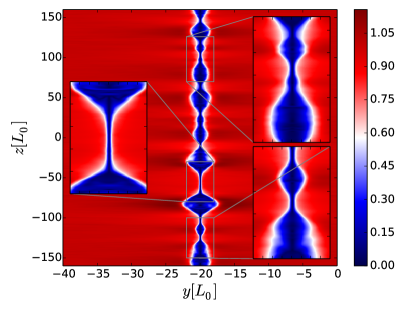
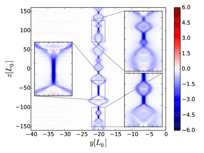
a) Magnetic field $\bf{B}$	b) Current density $\bf{J}$
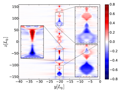
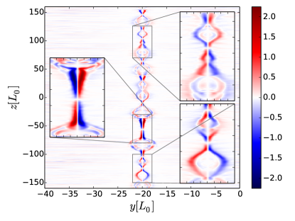
c) Outflow velocity $\bf{V}_{z}$	d) Vorticity $\bf{\Omega}$

Figure 2: Spatial distribution of the filtered field at $t=100\tau_{A}$ in the Harris-type CS equilibrium with $b_{g}=0$

The smaller reconnection rates in the first 100 $t/\tau_{A}$ in force-free equilibria can be related to the slightly lower maximum value of the current density $\boldsymbol{J}$ and mean vorticity $\boldsymbol{\Omega}$. The amplitude of these mean variables represent the stress felt by the mean magnetic and velocity fields, i.e., the strength of the gradients on these mean fields.

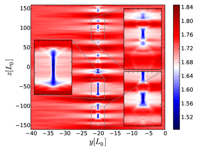
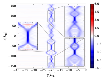
a) Magnetic field $\bf{B}$	b) Current densitiy $\bf{J}$
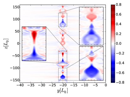
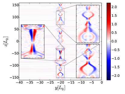
c) Outflow velocity $\bf{V}_{z}$	d) Vorticity $\bf{\Omega}$

Figure 3: Spatial distribution of the filtered field at $t=100\tau_{A}$ in the force-free CS equilibrium $b_{g}=2$.

Magnetic reconnection releases critically stressed magnetic fields and the stress strength at ’X’-point locations is related to the reconnection rate.Tsiklauri and Haruki (2007) A Harris-type CS equilibrium is unchanged by an additional out-of-plane constant guide magnetic field. On the other hand, a force-free current sheet has an initial in-plane current density which is reduced by the addition of a constant out-of-plane guide field. Hence, an increase of the guide magnetic field strength reduces the Lorentz force component due to the in-plane currents but not its total amplitude. In most astrophysical plasmas a guide magnetic field can exceed the anti-parallel reconnection magnetic field component (e.g.: in the solar corona). The reconnection rate can be estimated by dimensional analysis of the Lorentz force (Appendix B). At the boundary layer of the CS where the electric field identically vanishes $\overline{\bf{J}}\approx\overline{\bf{V}}\times\overline{\bf{B}}/\eta$. The guide magnetic field influence on the reconnection rate can be described as

$$M_{A,b_{g}}=M_{A}\left(\frac{\overline{B_{z}^{2}}}{\overline{B_{x}^{2}}+\overline{B_{z}^{2}}}\right)^{2},$$ (23)

where $\overline{B_{x}}$ is the out-of-plane component of the magnetic field (guide field) and $\overline{B_{z}}$ the reconnecting component of the magnetic field. $M_{A}$ represents the estimated value of the reconnection rate when no guide magnetic field is considered. A larger guide magnetic field decreases the reconnection rate as found in our simulations. This was also observed in other numerical simulations and laboratory experiment.Ni et al. (2015); Ricci, Lapenta, and Brackbill (2004); Tharp et al. (2013)
A turbulent helicity can be generated due to guide magnetic field effects. Hence, the guide magnetic field can be related to turbulence by the turbulent energy, turbulent cross-helicity and turbulent helicity. The influence of the magnetic stress on the mean magnetic and velocity fields and the turbulent reconnection rate by turbulence is discussed in the following sections.

IV Effect of turbulence on plasmoid reconnection

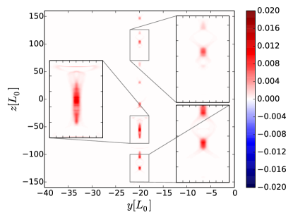
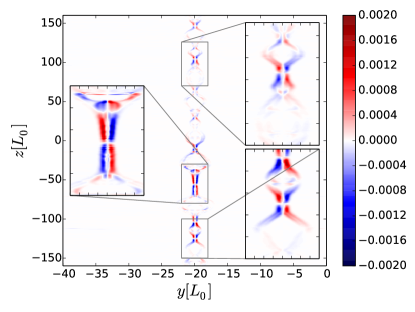
a) Turbulent energy $K$	b) Turbulent cross-helicity $W$
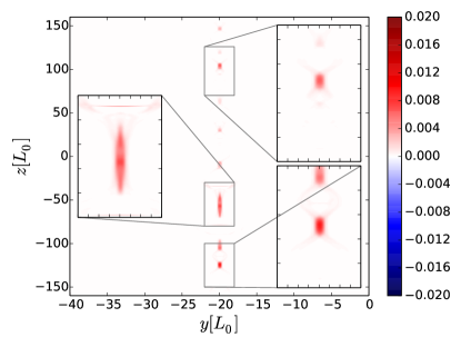
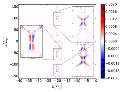
c) Turbulent energy $K$	d) Turbulent cross-helicity $W$

Figure 4: Spatial distribution of the turbulent energy $K$, cross-helicity $W$ at $t=100\tau_{A}$ in the Harris with $b_{g}=0$ ( a) and b) ) and force-free with $b_{g}=2$ ( c) and d)).

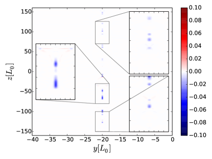
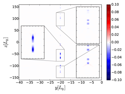
a) $H_{kin}$ Harris $b_{g}=2$	b) $H_{kin}$ force-free $b_{g}=2$
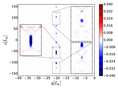
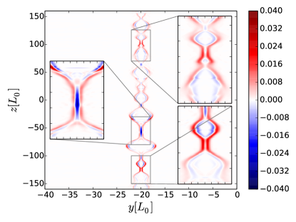
c) $H_{mag}$ Harris $b_{g}=2$	d) $H_{mag}$ force-free $b_{g}=2$
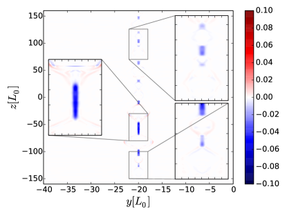
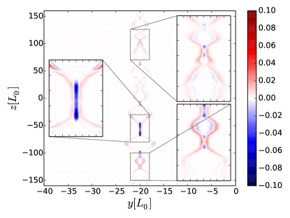
e) $H$ Harris $b_{g}=2$	f) $H$ force-free $b_{g}=2$

Figure 5: Spatial distribution of the turbulent kinetic helicity $H_{kin}$, magnetic helicity $H_{mag}$ and the total residual helicity at $t=100\tau_{A}$ in Harris with $b_{g}=2$ ( a), c) and e)) and force-free with $b_{g}=2$ ( b), d) ) and f)).

The dynamic balance of the turbulence quantities in the course of plasmoid unstable CSs is investigated by calculating the mean turbulent energy, turbulent cross-helicity and turbulent helicity obtained for the Gaussian filter formulation from the RANS turbulence model. The mean electric field equation is modified by the SGS model electromotive force ${\cal{E}}_{M}$ following Eq. (13) as

$$\overline{\bf{E}}=-\overline{\boldsymbol{V}}\times\overline{\boldsymbol{B}}+\left(\eta+\beta\right)\overline{\bf{J}}-\gamma\overline{\boldsymbol{\Omega}}-\alpha\overline{\boldsymbol{B}}$$ (24)

leading to the following mean induction equation

$$\partial_{t}\overline{\boldsymbol{B}}=\nabla\times\left(\overline{\boldsymbol{V}}\times\overline{\boldsymbol{B}}+\gamma\overline{\boldsymbol{\Omega}}+\alpha\overline{\boldsymbol{B}}-\beta\overline{\boldsymbol{J}}\right)+\eta\nabla^{2}\overline{\boldsymbol{B}}.$$ (25)

Equation (24) is used to obtain the current density $\overline{\bf{J}}$ which crossed with the mean magnetic field $\overline{\bf{B}}$ yields the following mean Lorentz force

$$\overline{\bf{J}}\times\overline{\bf{B}}=\frac{1}{\eta+\beta}\left(\overline{\bf{E}}\times\overline{\bf{B}}+\left(\overline{\bf{V}}\times\overline{\bf{B}}\right)\times\overline{\bf{B}}+\gamma\overline{\bf{\Omega}}\times\overline{\bf{B}}\right).$$ (26)

The amplitude of the turbulent resistivity $\beta$ and that of the $\gamma$ term related to the turbulent cross-helicity control the Lorentz force around the diffusion region of reconnection where they are finite. For high Reynolds number plasmas, the turbulent Reynolds number $R_{\beta}\sim 1/\beta$ is lower than the molecular one $R_{\eta}\sim 1/\eta$. In such a situation, the Lorentz force is decreased by an increased turbulence. The size of the diffusion region is enlarged and the reconnection rate is enhanced. The turbulent heicity $H$ related to the $\alpha$ term does not enter Eq. (26) directly but through its effect on the production of the turbulent energy and the turbulent cross-helicity which are both related to the $\beta$ and $\gamma$ terms. The turbulent helicity $H$ reduces the strength of the turbulent energy $K$. The turbulent resistivity $\beta$ is reduced and the Lorentz force is increased. As a result, the size of the diffusion region is diminished and the reconnection rate is slowed down. This way the mean Lorentz force, as well as Eq. (23), is directly related to the turbulence dynamics.
Our simulations show that the turbulent energy $K$ is located near the mean current density $\boldsymbol{J}$ concentration. Reconnection is enhanced by the turbulent resistivity $\beta$ related to $K$. The cross-helicity $W$, on the other hand, appears to be distributed around the current density maxima due to the mean vorticity $\boldsymbol{\Omega}$. This is true for all initial equilibria considered (Fig. 4) as theoretically predicted.Yokoi (2013)
In addition to the energy and cross-helicity of the turbulence, a turbulent helicity is generated as soon as an out-of-plane guide magnetic field is considered. According to its definition [Eq. (17)], the total mean turbulent helicity consists of kinetic and magnetic contributions

$$H_{tot} = -H_{kin}+H_{mag}$$ (27)

$$= -\left(\overline{\bf{V\cdot\Omega}}-\overline{\bf{V}}\cdot\overline{\bf{\Omega}}\right)+\left(\frac{\overline{\bf{B\cdot J}}-\overline{\bf{B}}\cdot\overline{\bf{J}}}{\bar{\rho}}\right)$$ (28)

An anti-parallel Harris-type CS equilibrium does not produce any turbulent helicity due to mirror-symmetry. A guide magnetic field can be added, however, to a Harris-type CS without changing its equilibrium. It produces initially a turbulent magnetic helicity $H_{mag}$ due to the alignment of the guide field and the mean current density (mirror-symmetry broken). The initial force-free CS equilibrium produces a force directed out of the reconnection plane which aligns of the mean velocity and vorticity field. It generates a kinetic helicity $H_{kin}$ in addition to a magnetic helicity $H_{mag}$. The initial conditions for the force-free equilibrium produced, therefore, both kinetic ($H_{kin}$) and magnetic ($H_{mag}$) turbulent helicity while a Harris-type CS equilibrium with guide field initially only generates a turbulent magnetic helicity ($H_{mag}$). Even though in a Harris-type CS with guide field there is no turbulent kinetic helicity present initially, it is later generated during the non-linear evolution of the reconnecting current sheet (Fig. 5). In both Harris-type and force-free CSs, the turbulent magnetic and kinetic helicity are located mainly at and near the ’X’-points of reconnection. Its location at the ’X’-point is due to the magnetic contribution $H_{mag}$. On the other hand, the distribution of the total turbulent helicity near the ’O’-points is a consequence of its kinetic contribution $H_{kin}$. Hence, the guide magnetic field is the reason for an increase of the total turbulent helicity $H_{tot}$. This relates the maximum reconnection rate to the guide field strength.
A strong guide field slows the reconnection rate [Eq. (23)]. This reduction can be attributed to the turbulent helicity $H$ related to the $\alpha$ term in Eq. (13). Its influence on the rate of magnetic reconnection can be obtained by the Alfvén Mach number $M_{A}$. Supposing steady state reconnection at each ’X’-point, a dimensional analysis reveals

$$M_{A}^{2}=\eta_{\ast}+\beta_{\ast}\left(1-\frac{|\gamma_{\ast}|+|\alpha_{\ast}|}{\beta_{\ast}}\eta_{\ast}^{1/2}\right).$$ (29)

The _∗ indicates that only the dimensions of the variables are used for the derivation. The normalisation is given by the Alfvén speed $V_{A}$ and the half-width $L_{0}$ for $\eta_{\ast}$, $\beta_{\ast}$ and $\gamma_{\ast}$. The $\alpha_{\ast}$ term is normalised by $V_{A}$. The reconnection rate decreases as soon as the $\alpha_{\ast}$ term is finite. This effect can be traced back to Eq. (13), where the influence of the turbulent resistivity ($\beta_{\ast}$) is attenuated by the turbulent helicity ($\alpha_{\ast}$). In fact, the turbulent helicity, as well as the turbulent cross-helicity, reduces the production of turbulent energy.Yokoi, Higashimori, and Hoshino (2013) The cross-helicity localises the turbulent energy near the ’X’-points in the diffusion region by suppressing its production around it. It is further suppressed by the turbulent helicity at the ’X’-points. This suppression of the apparent turbulent resistivity $\beta$ reduces the reconnection rate. This relates the rate of energy conversion in guide field reconnection to the turbulence dynamics.

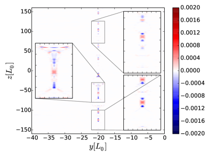
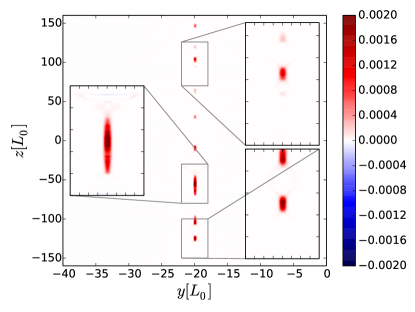
a) ${\cal{E}}$, Harris $b_{g}=0$	b) Model ${\cal{E}}_{M}$, Harris $b_{g}=0$
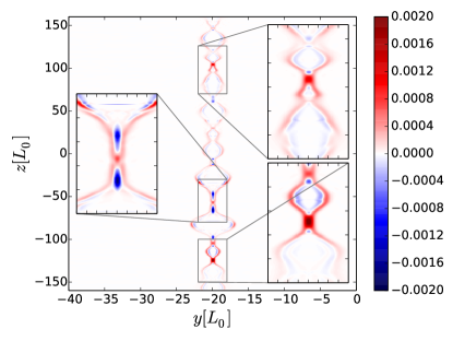
c) ${\cal{E}}$, force-free $b_{g}=2$	d) Model ${\cal{E}}_{M}$, force-free $b_{g}=2$

Figure 6: Spatial distribution at $100t/\tau_{A}$ of the electromotive force $\cal{E}$ and its modelling ${\cal{E}}_{M}$ in Harris-type CS $b_{g}=0$ a) and b)) and force-free CS $b_{g}=2$ ( c) and d)). The intensity of ${\cal{E}}$ is multiplied by a factor of two for visualisation purposes.

IV.1 Electromotive force

The electromotive force $\cal{E}$ is compared to the model ${\cal{E}}_{M}$ (Fig. 6). In anti-parallel Harris-type CS, the ${\cal{E}}_{M}$ is located at and around the ’X’-points similarly to the electromotive force ${\cal{E}}$. The amplitude of ${\cal{E}}_{M}$ is of the same order as the mean electromotive force but does, however, not reproduce the negative value near the ’O’-points. As soon as an out-of-plane guide magnetic field is considered in Harris-type CS, both the negative and positive signs of the electromotive force are recovered by ${\cal{E}}_{M}$. The turbulent helicity, generated after the mirror-symmetry breakage by the guide magnetic field, contributes to the negative sign of ${\cal{E}}_{M}$. The model ${\cal{E}}_{M}$ is, however, overestimating the electromotive force ${\cal{E}}$ calculation by a factor of three. The force-free CS shows similar results. Two reasons can be responsible for the overestimation. First the constants $C_{\alpha}$, $C_{\beta}$ and $C_{\gamma}$ influence the result. While $C_{\beta}$ and $C_{\gamma}$ are well established for the model under consideration, the value of $C_{\alpha}$ is not well known.Hamba (1992) On the other hand, the same turbulence timescale $\tau$ is chosen for all three turbulence variables $\beta$, $\gamma$ and $\alpha$. In fact it should be defined by the turbulence dynamics itself. On average over all reconnection site, the model electromotive force ${\cal{E}}_{M}$ corresponds to the behavior of $\cal{E}$ (Fig. 7).

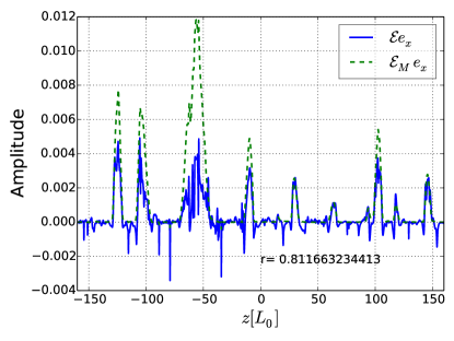
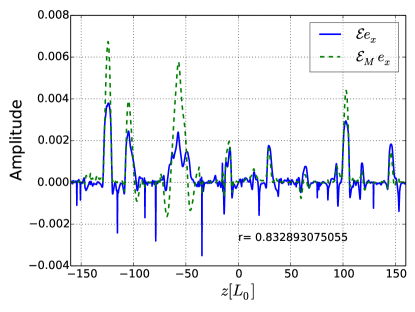
a) Harris $b_{g}=0$, $r=0.81$	b) Force-free $b_{g}=2$, $r=0.83$

Figure 7: Comparison of the electromotive forces along the center of the CS at $t=100\tau_{A}$ with correlation factor $r$ for a) Harris-type CS $b_{g}=0$, b) force-free $b_{g}=2$. Solid line: ${\cal{E}}$. Dashed line: ${\cal{E}}_{M}$. The model ${\cal{E}}_{M}$ is rescaled by 3 to be in the range of the electromotive force definition ${\cal{E}}$.

IV.2 Energy Consideration

In our Gaussian filter approach, the mean energy density of the magnetic field $\overline{{\bf{B}}^{2}}/2\mu_{0}$ can be split into its mean $\overline{{\bf{B}}}^{2}$ and its fluctuation part $\overline{{\bf{b}}^{\prime 2}}$. The evolution equation for the former is

$$\frac{d}{dt}\int\limits_{V}\frac{\overline{\bf{B}}^{2}}{2\mu_{0}}d\boldsymbol{x}=\int\limits_{V}\left[-\eta\overline{\bf{J}}^{2}-\overline{\bf{V}}\cdot(\overline{\bf{J}}\times\overline{\bf{B}})+\overline{\bf{J}}\cdot{\cal{E}}\right]\ d\boldsymbol{x},$$ (30)

where, depending on its sign, the last term on the right-hand side may be a source or a sink of energy. A stretching of field lines increases the magnetic energy while a contraction decreases it. Figure 8 a) depicts the evolution of the total magnetic energy and b) of the total kinetic energy within the simulation box. Note that the magnetic energy of the force-free equilibria is rescaled by a factor of three to be in the same range as the Harris-type CSs energy. While the magnetic energy rapidly decreases in Harris-type CSs without guide magnetic field, a force-free equilibrium with guide magnetic field retains a high level of magnetic energy. On the other hand, the plasma kinetic energy is lower for force-free CSs compared with anti-parallel Harris-type CS ($b_{g}=0$).

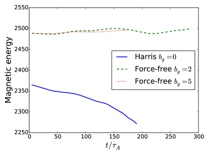
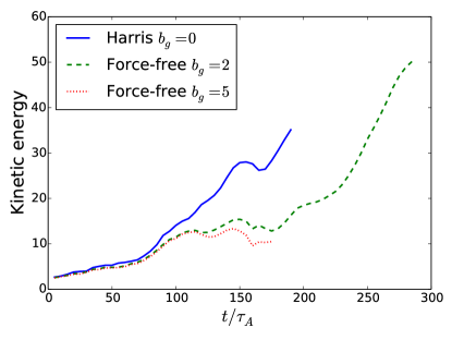
a) Magnetic energy	b) Kinetic energy

Figure 8: Time history of a) the total magnetic energy and b) the total kinetic energy. The energies are computed for the Harris-type current sheet without guide field and force-free current sheet with guide magnetic field $b_{g}=2$ and 5.

The electromotive force is positive near ’X’-points and negative near ’O’-points (Fig. 6). From turbulence viewpoint, the apparent turbulent resistivity $\beta$ is positive at and around the ’X’-points. Since the mean current $\overline{\bf{J}}$ is negative in the present geometry, the first term in Eq. (13) is positive at the ’X’-points where the current density accumulates the most. At the ’O’-point vicinity, the residual turbulent helicity is found to be negative for a positive guide magnetic field, the last term in Eq. (13) is then negative. The product $\overline{\bf{J}}\cdot\cal{E}$ is then negative close to the ’X’-points while it is positive close to the ’O’-points due to the balance of turbulence dynamics. The electromotive force causes a decrease of the magnetic energy at ’X’-points enhancing its conversion into the kinetic energy and heat. Near the ’O’-points, it causes an increase of the magnetic energy, converting the kinetic (plasma flow) energy into the magnetic energy and heat. Hence, the total kinetic energy is reduced and the total magnetic energy is increased there (Fig. 8). The modeled ${\cal{E}}_{M}$ [Eq. (13)] behaves similarly: the turbulent energy related to the $\beta$ term enhances the annihilation of magnetic energy while the $\gamma$ term (depending on its sign) together with the $\alpha$ term acts like a source term for the magnetic energy. The dynamical balance of turbulence modifies the contribution of the electromotive force to the mean magnetic energy. In Fig. 9, the different terms contributing to the right-hand side of Eq. (25) are shown for a given time as they are distributed along the current sheet. Figure 9 presents the result for the force-free equilibrium with $b_{g}=2$ but similar results are obtained for the other CS configurations and guide magnetic field strengths. The gradients of the turbulent helicity ($\alpha$ related term) and the turbulent resistivity $\beta$ cause important effects. The $\alpha$ term acts against the turbulent ($\beta$) and molecular ($\eta$) resistivity. In some locations, the turbulent helicity suppresses the turbulent diffusion ($\beta$ term), only the Joule dissipation ($\eta$) can convert the magnetic energy into heat. On the other hand, there is no mechanism to produce turbulent helicity in two dimensional Harris-type CSs without guide field since mirror-symmetry is not broken. The turbulent cross-helicity is the only source term for the magnetic energy near ’O’-points. The production of magnetic energy near the ’O’-points is, however, less than the counterpart in presence of turbulent helicity.

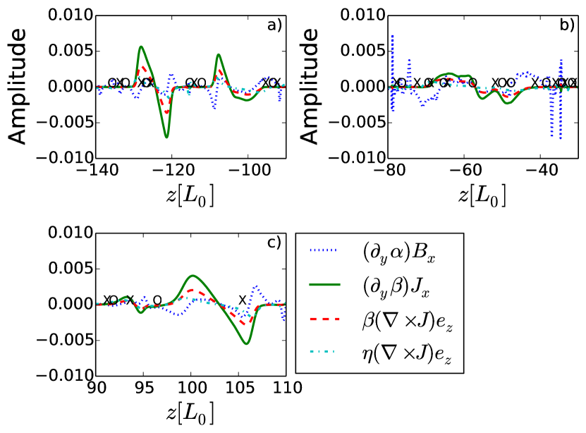
Figure 9: Components of the diffusion and advection terms along the current sheet from the mean induction equation. They correspond to the zoomed regions of reconnection in Fig. 3: a) the lower right zoom, b) the middle left zoom and c) the upper right zoom. The X and O denote the ’X’- and ’O’-points. The amplitude is multiplied by 100.0 for visualisation purposes.

In such a situation, the annihilation of the mean magnetic field is enhanced by the turbulent resistivity $\beta$ because no turbulent helicity ($\alpha$ related term), neither kinetic or magnetic, effects take place. There is no mechanism to reduce the turbulent energy at the ’X’-points and magnetic reconnection can grow fast.

IV.3 Turbulence relation to mean fields

For a reconnecting current sheet, the relation between turbulence and the ratio $|\boldsymbol{\Omega}|/|\boldsymbol{J}|$ was shown to be related to the reconnection rate.Yokoi and Hoshino (2011); Widmer, Büchner, and Yokoi (2016) The amount of turbulence in the system, represented by $|\gamma|/\beta$ in the Reynolds averaged turbulence model, can be estimated as

$$\left(\frac{|\gamma|}{\eta_{T}}\right)\cong M_{A}\frac{|\boldsymbol{J}_{\star}|}{|\boldsymbol{\Omega}|},$$ (31)

where $\boldsymbol{J}_{\star}=(\boldsymbol{J}\sqrt{\mu_{0}})/\sqrt{\rho}$ and $\eta_{T}=\eta+\beta$. In the limit of $\beta\gg\eta$, it is mainly the turbulent diffusivity $\beta$ that determines the denominator. In this limit, the turbulence dominates the dissipation of magnetic energy in the diffusion regions [Eq. (29)]. The estimated amount of turbulence can be compared with the actual level obtained by the filtered $K$ and $W$. Figure 10 shows the time history of the amount of turbulence estimated by Eq. (31) and calculated from the filtered $K$ and $W$ with $\tau=1$, $C_{\beta}=0.05$, $C_{\gamma}=0.04$ and $C_{\alpha}=0.02$. For this set of parameters, the estimation (31) is in quiet good agreement with the ratio computed directly from $\gamma$ and $\beta$.

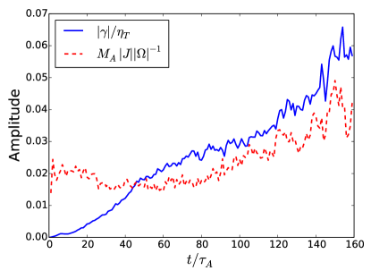
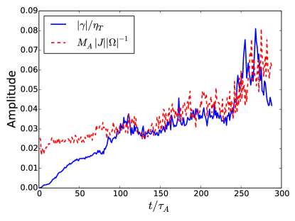
a)	b)

Figure 10: Time history of the amount of turbulence in the system according to the RANS model. a) Harris-type and b) Force free with $b_{g}=2$. Dashed line: calculated from Eq. (31). Solid line: the ratio of the filtered turbulence quantities

Finally, the reconnection rate determined as before as the averaged out-of-plane electric field $|E_{x}|$ at the ’X’-points is compared with

$$M_{A}=\frac{|\boldsymbol{\Omega}|}{|\boldsymbol{J}_{\star}|}\left(\frac{|\gamma|}{\eta_{T}}\right).$$ (32)

The reconnection given by Eq. (32) corresponds well with the value directly obtained by the out-of-plane electric field $|E_{x}|$ (Fig. 11).

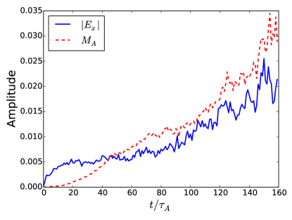
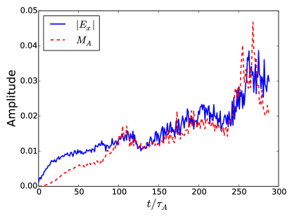
a) Harris, $b_{g}=0$	b) Force free, $b_{g}=2$

Figure 11: Time history of the reconnection rate $|E_{x}|$ compared with the prediction $M_{A}$ of Eq. (32) for a) Harris-type current sheet with $b_{g}=2$ and b) force free equilibrium with $b_{g}=2$.

According to the Sweet-Parker (SP) scaling, the reconnection rate reduces as $\eta$ decreases: $M_{A}\propto S^{-1/2}\sim\eta^{1/2}$. Long current sheets unstable to plasmoid instability show, however, an independence of the reconnection rate with respect to the Reynolds number.Bhattacharjee et al. (2009) Since turbulence is ubiquitous at large Reynolds number plasmas (small $\eta$), the deviation from the SP scaling can be attributed to turbulence. Following Eq. (29), the reconnection rate is determined by turbulence at small molecular resistivity $\eta$. Figure 12 shows the deviation from the SP scaling (solid line) of the reconnection as well as the amount of turbulence calculated as Eq. (31). The turbulence saturates and the deviation from the SP scaling can be attributed to turbulence as well.

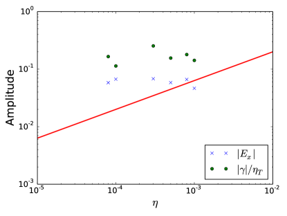
Figure 12: Time average of the reconnection rate $|E_{x}|$ and amount of turbulence $|\gamma|/\eta_{T}$ [Eq. (31)] for different molecular resistivity $\eta$. There is a deviation from the Sweet-Parker scaling as $\eta$ decreases. The reconnection rate and the turbulence saturate similarly. Solid line: Sweet-Parker scaling.

V Discussion and conclusions

We utilized a Reynolds averaged turbulence model in order to investigate the influence of small scale MHD turbulence on the plasmoid instability of long current current sheets in weakly dissipative plasmas. For this sake we first validated the applicability of this turbulence model by filtering the data obtained by high resolution simulations of plasmoid-unstable Harris-type and force-free current sheets in the presence of finite guide fields with different strength. We found that the energy of the turbulence $K$ is growing mainly near ’X’-points in the dissipation region of magnetic reconnection. There it causes additional, apparent "turbulent resistivity" (a $\beta$ -effect). The cross-helicty of the turbulence $W$ is growing around the ’X’-points where it forms in a quadrupolar structure with signs following the mean vorticity. This constrains the turbulent resistivity $\beta$ near the ’X’-points, enhancing the rate of magnetic reconnection. The turbulent helicity is growing, following the out-of-the-reconnection-plane (guide-) magnetic field, both near the ’X’- and ’O’-points. While near the ’X’-points the produced turbulent helicity is mainly magnetic ($H_{mag}$), it is mainly a kinetic turbulent helicity $H_{kin}$ which is produced at the ’O’-points (Fig. 13).

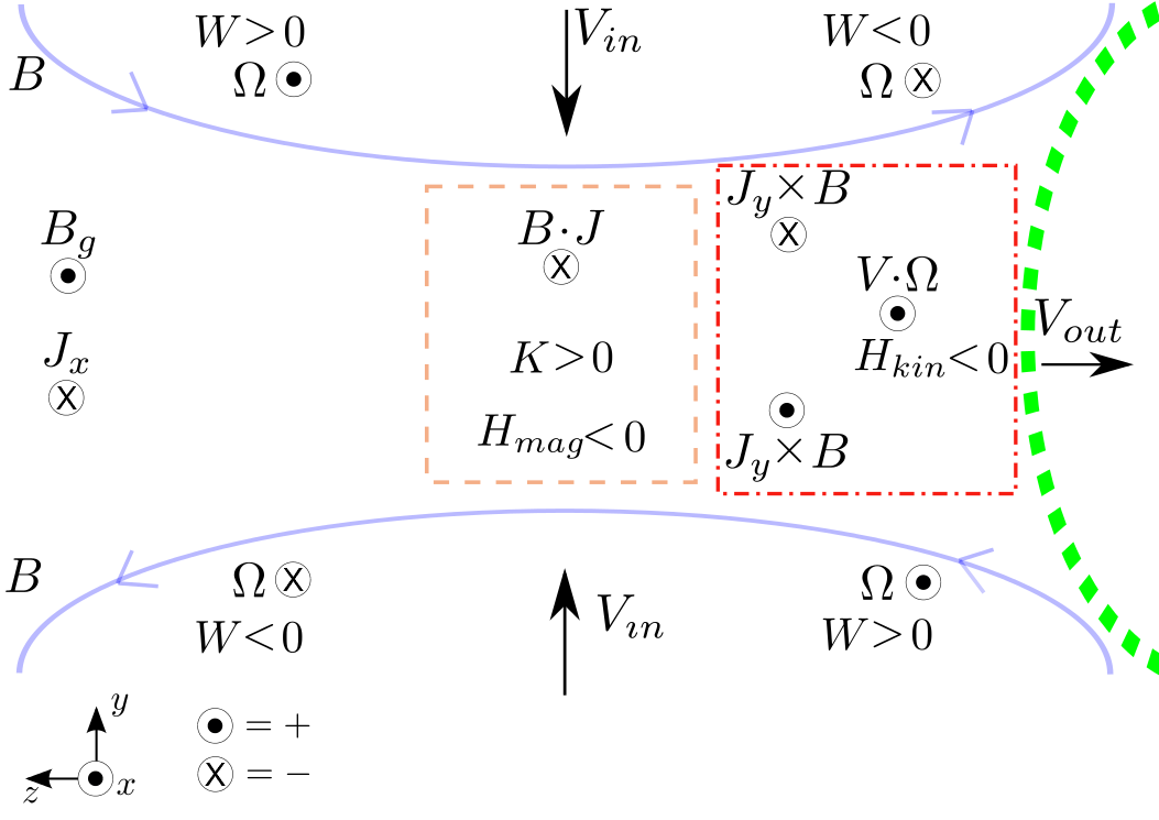
Figure 13: Schematic representation of an ’X’-point. The turbulent cross-helicity $W$ has the same sign as the mean vorticity $\Omega$. The dashed box represents the region near the ’X’-point. There the turbulent magnetic helicity is negative as $\overline{\bf{B}}\cdot\overline{\bf{J}}<0$ and the turbulent energy $K>0$. The line dashed box represents the region close to an ’O’-point (curved dashed line). The mean current $\overline{\bf{J_{y}}}$ produced by the guide magnetic field generates a force $\overline{\bf{J_{y}}}\times\overline{\bf{B}}$. It generates a velocity in the ${\bf{e_{x}}}$ direction. The turbulent kinetic helicity is negative since $-\overline{\bf{V}}\cdot\overline{\bf{\Omega}}<0$.

As a result the turbulent kinetic helicity converts near ’O’-points plasma kinetic energy into magnetic energy and heat. This increases the total mean magnetic energy which then retains a high level even though reconnection takes place. Note that the turbulent-helicity related $\alpha$ term can reduce the turbulent and resistive annihilation of magnetic flux near ’X’-points if a guide field breaks the mirror-symmetry of a pure Harris-type current sheet with anti-parallel magnetic fields only. At ’X’-points the apparent effective turbulent resistivity $\beta$ can become, therefore, balanced by turbulent helicity effects which slows down the conversion of magnetic into kinetic energy and reduces the reconnection rate compared to the case of anti-parallel Harris-type current sheets with vanishing guide fields ($b_{g}=0$). A reduction of the reconnection rate in presence of large guide magnetic field can, therefore, be explained by means of turbulent helicity.
The modelled electromotive force ${\cal{E}}_{M}$ which depends on the energy of the turbulence $K$, the turbulent cross-helicity $W$ and the turbulent helicity $H$, agrees with the statistically determined $\cal{E}$. It is, however, about three times larger than the calculated electromotive force. In fact, in the course of plasmoid reconnection many differently sized islands are formed while in our model we choose the same constant turbulence timescale for all reconnection sites without taking into account their correlation. As it previously was found for single ’X’-point, turbulent reconnection becomes fast if the turbulence time scale is of the order of the Alfvén crossing time $\tau_{A}$. Higashimori, Yokoi, and Hoshino (2013); Widmer, Büchner, and Yokoi (2016) A choice of constant turbulence time scale is, therefore, a good approximation. The mean field turbulence model was, therefore, found to apply not only to the problem of single ’X’-point but also for cascading plasmoid-type reconnection.
According to the model, the turbulence is driven by the inhomogeneities of the large scale (mean-) fields, current density and vorticity. The mean fields and the ratio of turbulent energy to the turbulent cross-helicity determine the reconnection rate calculated as the out-of-plane mean electric field at the ’X’-points. The deviation of the reconnection rate from the Sweet-Parker scaling is found to be related to the saturation of the SGS turbulence. The proposed Reynolds-averaged turbulence model is, therefore, able to reproduce the consequences of SGS effects for the reconnection rate of turbulent plasmoid-unstable current-sheet reconnection as well as its deviation from the Sweet-Parker scaling. The SGS turbulence model reproduces the macroscopic electromotive force and explain its dependencies. The model also allows to describe guide magnetic field effects controlling the turbulent helicity $H$ and its influence on the energy conversion rate.

Appendix A Effects of the Filter Width

The mean field quantities are calculated by means of a Gaussian filter. Such a filter cannot, however, strictly fulfill Reynolds rules, i.e., $\left<f^{\prime}\right>\neq 0$. This means that cross-terms such as $\overline{\bf{v^{\prime}\times B}}$ may have important influence on the results. To avoid such issues, mean field are usually defined by global average. This cannot be done in 2.5D simulations because the spatial variations of the mean fields describing the substructures of the current sheet are required. A time average can not be carried out either, as a steady state is not reached properly. To reduce the effect of the cross-terms, different filter widths have been tested. Applying the filter on the Reynolds decomposition of a physical quantity $f$ gives

$$\overline{f}=\overline{\overline{f}}+\overline{f^{\prime}},$$ (33)

where the over line correspond to a filtered quantity. The mean field is considered to be $\overline{f}$. To apply Reynolds rules, $\overline{f^{\prime}}/\overline{\overline{f}}$ should be as close to zero as possible and $\overline{f}/\overline{\overline{f}}$ should be close to one. Figure 14 shows that an increased filter width increases both ratios values. In our calculation, the filter width was chosen such that these ratios are close enough to fulfill Reynolds rules while turbulence quantities is still sufficiently spatially resolved. The chosen width in normalised unit is 5.

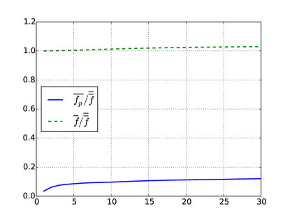
Figure 14: Amplitude of the box average of the ratio $\overline{f^{\prime}}/\overline{\overline{f}}$ and $\overline{f}/\overline{\overline{f}}$ with respect to the filter width. $f_{p}\equiv f^{\prime}$

Appendix B Heuristic derivation of the Lorentz Force

The electric field vanishes identically at the current sheet (CS) boundary. This provides $\overline{\bf{J}}\cong\overline{\bf{V}}\times\overline{\bf{B}}/\eta$. The Lorentz force components across the CS for both guide field and non guide field equilibrium are (over lines are omitted)

$$\overline{F_{L}}\bf{e_{y}}=\left\{\begin{array}[]{rcl}\left(-V_{y}B_{z}^{2}+V_{z}B_{y}B_{z}-V_{y}B_{x}^{2}\right)/\eta&\mbox{for}&B_{x}\neq 0\\ \left(-V_{y}B_{z}^{2}+V_{z}B_{y}B_{z}\right)/\eta&\mbox{for}&B_{x}=0\end{array}\right.$$ (34)

where the guide field is represented by the component $B_{x}$. When a magnetic field line changes its topology at the ’X’-point, it is assumed that $\overline{F_{L}}\bf{e_{y}}\equiv 0$. This condition yields

$$\overline{F_{L}}\bf{e_{y}}=\left\{\begin{array}[]{rcl}\frac{V_{y}}{V_{z}}=\frac{B_{y}B_{z}}{B_{z}^{2}+B_{x}^{2}}&\mbox{for}&B_{x}\neq 0\\ \frac{V_{y}}{V_{z}}=\frac{B_{y}}{B_{z}}&\mbox{for}&B_{x}=0\end{array}\right.$$ (35)

We finally obtain from the definition of the Alfvén Mach number $M_{A}=V_{y}^{2}/V_{z}^{2}$ the relation

$$M_{A,b_{g}}=M_{A}\left(\frac{B_{z}^{2}}{B_{z}^{2}+B_{x}^{2}}\right)^{2},$$ (36)

where $M_{A,b_{g}}$ and $M_{A}$ are the reconnection rates for guide field and non-guide field CS equilibria.