Methods for Sparse and Low-Rank Recovery under Simplex Constraints

Abstract

The de-facto standard approach of promoting sparsity by means of $\ell_{1}$-regularization becomes ineffective in the presence of simplex constraints, i.e., the target is known to have non-negative entries summing up to a given constant. The situation is analogous for the use of nuclear norm regularization for low-rank recovery of Hermitian positive semidefinite matrices with given trace. In the present paper, we discuss several strategies to deal with this situation, from simple to more complex. As a starting point, we consider empirical risk minimization (ERM). It follows from existing theory that ERM enjoys better theoretical properties w.r.t. prediction and $\ell_{2}$-estimation error than $\ell_{1}$-regularization. In light of this, we argue that ERM combined with a subsequent sparsification step like thresholding is superior to the heuristic of using $\ell_{1}$-regularization after dropping the sum constraint and subsequent normalization.

At the next level, we show that any sparsity-promoting regularizer under simplex constraints cannot be convex. A novel sparsity-promoting regularization scheme based on the inverse or negative of the squared $\ell_{2}$-norm is proposed, which avoids shortcomings of various alternative methods from the literature. Our approach naturally extends to Hermitian positive semidefinite matrices with given trace. Numerical studies concerning compressed sensing, sparse mixture density estimation, portfolio optimization and quantum state tomography are used to illustrate the key points of the paper.

1 Introduction

In this paper, we study the case in which the parameter of interest $\beta^{*}$ is sparse and non-negative with known sum, i.e., $\beta^{*}\in c\Delta^{p}\cap{\mathbb{B}}_{0}^{p}(s)$, where for $c>0$ and $1\leq s\leq p$, $c\Delta^{p}=\{\beta\in{\mathbb{R}}_{+}^{p}:\,\bm{1}^{\top}\beta=c\}$ is the (scaled) canonical simplex in ${\mathbb{R}}^{p}$, ${\mathbb{B}}_{0}^{p}(s)=\{\beta\in{\mathbb{R}}^{p}:\,\left\lVert\beta\right\rVert_{0}\leq s\}$ and $\left\lVert\beta\right\rVert_{0}=|S(\beta)|=|\{j:\,\beta_{j}\neq 0\}|$ is referred to as $\ell_{0}$-norm (the cardinality of the support $S(\beta)$). Unlike the constant $c$, the sparsity level $s$ is regarded as unknown. The specific value of the constant $c$ is not essential; in the sequel, we shall work with $c=1$ as for all problem instances studied herein, the data can be re-scaled accordingly. The elements of $\Delta^{p}$ can represent probability distributions over $p$ items, proportions or normalized weights, which are quantities frequently arising in instances of contemporary data analysis. A selection is listed below.

• Estimation of mixture proportions.      Specific examples are the determination of the proportions of chemical constituents in a given sample or the endmember composition of pixels in hyperspectral imaging (Keshava, 2003).

• Probability density estimation, cf. Bunea et al. (2010).      Let $(\mathcal{Z},\mathcal{A},P)$ be a probability space with $P$ having a density $f$ w.r.t. some dominating measure $\nu$. Given a sample $\{Z_{i}\}_{i=1}^{n}\overset{\text{i.i.d.}}{\sim}P$ and a dictionary $\{\phi_{j}\}_{j=1}^{p}$ of densities (w.r.t. $\nu$), the goal is to find a mixture density $\phi_{\beta}=\sum_{j=1}^{p}\beta_{j}\phi_{j}$ well approximating $f$, where $\beta\in\Delta^{p}$.

• Convex aggregation/ensemble learning.      The following problem has attracted much interest in non-parametric estimation, cf. Nemirovski (2000). Let $f$ be the target in a regression/classification problem and let $\{\phi_{j}\}_{j=1}^{p}$ be an ensemble of regressors/classifiers. The goal is to approximate $f$ by a convex combination of $\{\phi_{j}\}_{j=1}^{p}$.

• Markowitz portfolios (Markowitz, 1952) without short positions.      Given $p$ assets whose returns have expectation $r=(r_{1},\ldots,r_{p})^{\top}$ and covariance $\Sigma$, the goal is to distribute the total investment according to proportions $\beta\in\Delta^{p}$ such that the variance $\beta^{\top}\Delta\beta$ is minimized subject to a lower bound on the expected return $\beta^{\top}r$.

Sparsity is often prevalent or desired in these applications.

• In hyperspectral imaging, a single pixel usually contains few endmembers.

• In density estimation, the underlying density may be concentrated in certain regions of the sample space.

• In aggregation, it is common to work with a large ensemble to improve approximation capacity, while specific functions may be well approximated by few members of the ensemble.

• A portfolio involving a small number of assets incurs less transaction costs and is much easier to manage.

At the same time, promoting sparsity in the presence of the constraint $\beta\in\Delta^{p}$ appears to be more difficult as $\ell_{1}$-regularization does not serve this purpose anymore. As clarified in $\S$2, the naive approach of employing $\ell_{1}$-regularization and dropping the sum constraint is statistically not sound. The situation is similar for nuclear norm regularization and low-rank matrices that are Hermitian positive semidefinite with fixed trace as arising (e.g.,) in quantum state tomography (Gross et al., 2010), where the constraint set is given by $\bm{\Delta}^{m}=\{B\in{\mathbb{C}}^{m\times m}:B=B^{H},\,B\succeq 0,\,\operatorname*{tr}(B)=1\}$, where ^H denotes conjugate transposition. Both the presence of simplex constraints and its matrix counterpart thus demand different strategies to deal with sparsity and low-rankedness, respectively. The present paper proposes such strategies that are statistically sound, straightforward to implement, adaptive in the sense that the sparsity level $s$ (resp. the rank in the matrix case) is not required to be known, and that work with a minimum amount of hyperparameter tuning.

Related work. The problem outlined above is nicely discussed in Kyrillidis et al. (2013). In that paper, the authors consider the sparsity level $s$ to be known as well and suggest to deal with the constraint set $\Delta_{0}^{p}(s)=\Delta^{p}\cap{\mathbb{B}}_{0}^{p}(s)$ by projected gradient descent based on a near-linear time algorithm for computing the projection. This approach can be seen as a natural extension of iterative hard thresholding (IHT, Blumensath and Davies (2009)). It has clear merits in the matrix case, where significant computational savings are achieved in the projection step. On the other hand, it is a serious restriction to assume that $s$ is known. Moreover, the method has theoretical guarantees only under the restricted isometry property (RIP, Candes and Tao (2007)) and a certain choice of the step size depending on RIP constants, which are not accessible in practice.

Pilanci et al. (2012) suggest the regularizer $\beta\mapsto 1/\left\lVert\beta\right\rVert_{\infty}$ to promote sparsity on $\Delta^{p}$ and show that in the case of squared loss, the resulting non-convex optimization problem can be reduced to $p$ second-order cone programs. In practice, however, in particular when combined with tuning of the regularization parameter, the computational cost quickly becomes prohibitive.

Relevant prior work also includes Larsson and Ugander (2011) and Shashanka et al. (2008) who discuss the problem of this paper in the context of latent variable representations (PLSA, Hofmann (1999)) for image and bag-of-words data. Larsson and Ugander (2011) proposes a so-called pseudo-Dirichlet prior correponding to the log-penalty in Candes et al. (2007). Shashanka et al. (2008) suggest to use the Shannon entropy as regularizer. Both approaches are cumbersome regarding optimization due to the singularity of the logarithm at the origin which is commonly handled by adding a constant $\varepsilon>0$ to the argument, thereby introducing one more hyperparameter; we refer to $\S$4.4 below for a more detailed discussion.

A conceptually different approach is pursued in Jojic et al. (2011). Instead of the usual loss + $\ell_{1}$-norm formulation with the $\ell_{1}$-norm arising as the convex envelope (also known as bi-conjugate, cf. Rockafellar (1970), §12) of the $\ell_{0}$-norm on the unit $\ell_{\infty}$-ball, the authors suggest to work with the convex envelope of loss + $\ell_{0}$-norm. A major drawback is computational cost since evaluation of the convex envelope already entails solving a convex optimization problem.

Outline and contributions of the paper.

As a preliminary step, we provide a brief analysis of high-dimensionsal estimation under simplex constraints in $\S$2. Such analysis provides valuable insights when designing suitable sparsity-promoting schemes. An important observation is that empirical risk minimization (ERM) and elements of $\Delta^{p}$ contained in a “high confidence set” for $\beta^{*}$ (a construction inspired by the Dantzig selector of Candes and Tao (2007)) already enjoy nice statistical guarantees, among them adaptation to sparsity under a restricted strong convexity condition weaker than that in Negahban et al. (2012). This situation does not seem to be properly acknowledged in the work cited in the previous paragraph. As a result, methods have been devised that may not even achieve the guarantees of ERM. By contrast, we here focus on schemes designed to improve over ERM, particularly with respect to sparsity of the solution and support recovery. As a basic strategy, we consider simple two-stage procedures, thresholding and re-weighted $\ell_{1}$ regularization on top of ERM in §3.

Alternatively, we propose a novel regularization-based scheme in $\S$4 in which $\beta\mapsto 1/\left\lVert\beta\right\rVert_{2}^{2}$ serves as a relaxation of the $\ell_{0}$-norm on $\Delta^{p}$. This approach naturally extends to the matrix case (positive semidefinite Hermitian matrices of trace one) as discussed in $\S$5. On the optimization side, the approach can be implemented easily by DC (difference of convex) programming (Pham Dinh and Le Thi, 1997). Unlike other popular forms of concave regularization such as the SCAD, capped $\ell_{1}$ or MCP penalties (Zhang and Zhang, 2013) no extra parameter besides the regularization parameter needs to be specified. For this purpose, we consider a generic BIC-type criterion (Schwarz (1978); Kim et al. (2012)) with the aim to achieve correct model selection respectively rank selection in the matrix case. The effectiveness of both the two-stage procedures and the regularization-based approach is demonstrated by several sets of numerical experiments covering applications in compressed sensing, density estimation, portfolio optimization and quantum state tomography. All proofs can be found in the appendix.

Notation.

For the convenience of readers, we here gather essential notation. We denote by $\lVert\cdot\rVert_{q}$, $0\leq q\leq\infty$, the usual $\ell_{q}$-norm or the Schatten $\ell_{q}$-norm depending on the context, and by $\left\langle\cdot,\cdot\right\rangle$ the usual Euclidean inner product. We use $|\cdot|$ for the cardinality of a set. We write $\mathbf{I}(\cdot)$ for the indicator function. We denote by $\{e_{1},\ldots,e_{d}\}$ the canonical basis of ${\mathbb{R}}^{d}$. For $A\subseteq{\mathbb{R}}^{d}$, $\Pi_{A}:{\mathbb{R}}^{d}\rightarrow A$ denotes the Euclidean projection on $A$. For functions $f(n)$ and $g(n)$, we write $f(n)\gtrsim g(n)$ and $f(n)\lesssim g(n)$ to express that $f(n)\geq Cg(n)$ respectively $f(n)\leq Cg(n)$ for some constant $C>0$. We write $f(n)\asymp g(n)$ if both $f(n)\gtrsim g(n)$ and $f(n)\lesssim g(n)$. We also use the Landau symbols $O(\cdot)$ and $o(\cdot)$.

2 Simplex constraints in high-dimensional statistical inference: basic analysis

Before designing schemes promoting sparsity under the constraint $\beta\in\Delta^{p}$, it is worthwhile to derive basic performance bounds and to establish adaptivity to underlying sparsity when only simplex constraints are used for estimation, without explicitly enforcing sparse solutions. Note that the constraint $\beta\in\Delta^{p}$ is stronger than the $\ell_{1}$-ball constraint $\lVert\beta\rVert_{1}\leq 1$. As a consequence, it turns out that ERM enjoys properties known from the analysis of (unconstrained) $\ell_{1}$-regularized estimation, including adaptivity to sparsity under certain conditions. This already sets a substantial limit on what can be achieved in addition by sparsity-promoting schemes.

We first fix some notation. Let $\{Z_{1},\ldots,Z_{n}\}$ be i.i.d. copies of a random variable $Z$ following a distribution $P$ on some sample space $\mathcal{Z}\subseteq{\mathbb{R}}^{d}$. Let further $L:{\mathbb{R}}^{p}\times\mathcal{Z}\rightarrow{\mathbb{R}}$ a loss function such that $\forall z\in\mathcal{Z}$, $L(\cdot,z)$ is convex and differentiable. For $\beta\in{\mathbb{R}}^{p}$, $R(\beta)=\operatorname*{\mathbf{E}}[L(\beta,Z)]$ denotes the expected risk and $R_{n}(\beta)=n^{-1}\sum_{i=1}^{n}L(\beta,Z_{i})$ its empirical counterpart. The goal is to recover $\beta^{*}=\operatorname*{argmin}_{\beta\in\Delta^{p}}\operatorname*{\mathbf{E}}[L(\beta,Z)]$.

Besides ERM which yields $\widehat{\beta}\in\operatorname*{argmin}_{\beta\in\Delta^{p}}R_{n}(\beta)$, our analysis simultaneously covers all elements of the set

$$\mathcal{D}(\lambda)=\{\beta\in\Delta^{p}:\,\lVert\nabla R_{n}(\beta)\rVert_{\infty}\leq\lambda\},$$ (1)

for suitably chosen $\lambda\geq 0$ as precised below. The construction of $\mathcal{D}(\lambda)$ is inspired by the constraint set of the Dantzig selector (Candes and Tao, 2007), which is extended to general loss functions in Lounici (2008); James and Radchenko (2009); Fan (2013). Elements of $\mathcal{D}(\lambda)$ will be shown to have performance comparable to $\widehat{\beta}$. The set $\mathcal{D}(\lambda)$ need not be convex in general. For squared loss it becomes a convex polyhedron. It is non-empty as long as $\lambda\geq\lambda_{*}$, where $\lambda_{*}=\lVert\nabla R_{n}(\beta^{*})\rVert_{\infty}$. In many settings of interest (cf. Lounici (2008); Negahban et al. (2012)), it can be shown that

$$\vspace{-1ex}\operatorname*{\mathbf{P}}(\lambda_{*}\gtrsim\sqrt{\log(p)/n})=o(1)\;\;\,\text{as}\;n\rightarrow\infty.$$ (2)

2.1 Excess risk

The first result bounds the excess risk of $\widehat{\beta}$ and $\widetilde{\beta}_{\lambda}$, where in the sequel $\widetilde{\beta}_{\lambda}$ represents an arbitrary element of $\mathcal{D}(\lambda)$.

Proposition 1.

For $\beta\in{\mathbb{R}}^{p}$, let $\psi_{n}(\beta)=R_{n}(\beta)-R(\beta)$ and $\overline{\psi}_{n}(\beta)=\psi_{n}(\beta)-\psi_{n}(\beta^{*})$. For $r>0$, let ${\mathbb{B}}_{1}^{p}(r;\beta^{*})=\{\beta\in{\mathbb{R}}^{p}:\left\lVert\beta-\beta^{*}\right\rVert_{1}\leq r\}$ denote the $\ell_{1}$-ball of radius $r$ centered at $\beta^{*}$ and $\overline{\Psi}_{n}(r)=\sup\{|\overline{\psi}_{n}(\beta)|:\;\beta\in{\mathbb{B}}_{1}^{p}(r;\beta^{*})\}$. We then have

$$R(\widehat{\beta})-R(\beta^{*}) \leq\overline{\Psi}_{n}(\lVert\widehat{\beta}-\beta^{*}\rVert_{1})\leq\overline{\Psi}_{n}(2),$$

$$R(\widetilde{\beta}_{\lambda})-R(\beta^{*}) \leq\overline{\Psi}_{n}(\lVert\widetilde{\beta}_{\lambda}-\beta^{*}\rVert_{1})+\lambda\lVert\widetilde{\beta}_{\lambda}-\beta^{*}\rVert_{1}$$

$$\leq\overline{\Psi}_{n}(2)+2\lambda.$$

The excess risk of ERM and points in $\mathcal{D}(\lambda)$ can thus be bounded by controlling $\overline{\Psi}_{n}(r)$, the supremum of the empirical process $\overline{\psi}_{n}(\beta)$ over all $\beta$ with $\ell_{1}$-distance at most $r$ from $\beta^{*}$. This supremum is well-studied in the literature on $\ell_{1}$-regularization. For example, for linear regression with fixed or random sub-Gaussian design and sub-Gaussian errors as well as for Lipschitz loss (e.g. logistic loss), it can be shown that (van de Geer, 2008)

$$\operatorname*{\mathbf{P}}(\overline{\Psi}_{n}(r)\gtrsim r\sqrt{\log(p)/n})=o(1)\;\;\,\text{as}\;n\rightarrow\infty.$$ (3)

Using that $\widehat{\beta}\in\Delta^{p}$ and $\widetilde{\beta}_{\lambda}\in\Delta^{p}$, choosing $\lambda\asymp\lambda_{*}$ and invoking (2), Proposition 1 yields that the excess risk of ERM and points in $\mathcal{D}(\lambda)$ scales as $O(\sqrt{\log(p)/n})$. As a result, ERM and finding a point in $\mathcal{D}(\lambda)$ constitute persistent procedures in the sense of Greenshtein and Ritov (2004).

2.2 Adaptation to sparsity

Proposition 1 does not entail further assumptions on $\beta^{*}$ or $R_{n}$. In the present subsection, however, we suppose that $\beta^{*}\in\Delta_{0}^{p}(s)$ and that $R_{n}$ obeys a restricted strong convexity (RSC) condition defined as follows. Consider the set

$$\mathcal{C}^{\Delta}(s)=\{\delta\in{\mathbb{R}}^{p}:\;\exists J\subseteq\{1,\ldots,p\},|J|\leq s\;\,\,\,\text{s.t.}\;\bm{1}^{\top}\delta_{J^{c}}=-\bm{1}^{\top}\delta_{J},\;\;\delta_{J^{c}}\succeq 0\}.$$ (4)

Observe that $\{\beta-\beta^{*}:\;\beta\in\Delta^{p}\}\subseteq\mathcal{C}^{\Delta}(s)$. For the next result, we require $R_{n}$ to be strongly convex over $\mathcal{C}^{\Delta}(s)$.

Condition 1.

We say that the $\Delta$-RSC condition is satified for sparsity level $1\leq s\leq p$ and constant $\kappa>0$ if for all $\beta\in\Delta_{0}^{p}(s)$ and all $\delta\in\mathcal{C}^{\Delta}(s)$, one has

$$\vspace{-1ex}R_{n}(\beta+\delta)-R_{n}(\beta)-\nabla R_{n}(\beta)^{\top}\delta\geq\kappa\lVert\delta\rVert_{2}^{2}.$$

Condition 1 is an adaptation of a corresponding condition employed in Negahban et al. (2012) for the analysis of (unconstrained) $\ell_{1}$-regularized ERM. Our condition here is weaker, since the RSC condition in Negahban et al. (2012) is over the larger set

$$\mathcal{C}(\alpha,s)=\{\delta\in{\mathbb{R}}^{p}:\;\exists J\subseteq\{1,\ldots,p\},|J|\leq s\;\,\,\,\text{s.t.}\;\lVert\delta_{J^{c}}\rVert_{1}\leq\alpha\lVert\delta_{J}\rVert_{1}\},\;\,\text{for}\;\alpha\geq 1.$$

We are now in position to state a second set of bounds.

Proposition 2.

Suppose that the $\Delta$-RSC condition is satisfied for sparsity level $s$ and $\kappa>0$. We then have

$$\lVert\widehat{\beta}-\beta^{*}\rVert_{2}^{2}\leq\frac{4s\lambda_{*}^{2}}{\kappa^{2}},\quad\lVert\widetilde{\beta}_{\lambda}-\beta^{*}\rVert_{2}^{2}\leq\frac{4s(\lambda+\lambda_{*})^{2}}{\kappa^{2}},$$

$$\lVert\widehat{\beta}-\beta^{*}\rVert_{1}\leq\frac{4s\lambda_{*}}{\kappa},\quad\lVert\widetilde{\beta}_{\lambda}-\beta^{*}\rVert_{1}\leq\frac{4s(\lambda+\lambda_{*})}{\kappa}$$

Invoking (2) and choosing $\lambda\asymp\lambda_{*}$, we recover the rates $O(s\log(p)/n)$ for squared $\ell_{2}$-error and $O(s\sqrt{\log(p)/n})$ for $\ell_{1}$-error, respectively. Combining the bounds on $\ell_{1}$-error with (3) and Proposition 1, we obtain

$$R(\widehat{\beta})-R(\beta^{*})\lesssim\frac{s\log p}{n},\quad R(\widetilde{\beta}_{\lambda})-R(\beta^{*})\lesssim\frac{s\log p}{n}.$$

The above rates are known to be minimax optimal for the parameter set ${\mathbb{B}}_{0}^{p}(s)$ and squared loss (Ye and Zhang, 2010). Under the $\Delta$-RSC condition, there hence does not seem to be much room for improving over $\widehat{\beta}$ and $\widetilde{\beta}_{\lambda}$ as far as the $\ell_{1}$-error, $\ell_{2}$-error and excess risk are concerned. An additional plus of $\widehat{\beta}$ is that it does not depend on any hyperparameter.

3 Two-stage procedures

While $\widehat{\beta}$ has appealing adaptation properties with regard to underlying sparsity, $\lVert\widehat{\beta}\rVert_{0}$ may be significantly larger than the sparsity level $s$. Note that the $\ell_{2}$-bound of Proposition 2 yields that $S(\widehat{\beta})\supseteq S(\beta^{*})$ as long as $b_{\min}^{*}\gtrsim\lambda^{*}\sqrt{s}$, where $b_{\min}^{*}=\min\{\beta_{j}^{*}:\,j\in S(\beta^{*})\}$. If the aim is to construct an estimator $\widehat{\theta}$ achieving support recovery, i.e., $S(\widehat{\theta})=S(\beta^{*})$, $\widehat{\beta}$ needs to be further sparsified by a suitable form of post-processing. We here consider two common schemes, thresholding and weighted $\ell_{1}$-regularization. The latter is often referred to as “adaptive lasso” (Zou, 2006). Specifically, we define

thresholding: $$\quad\widehat{\beta}_{\tau}=(\widehat{\beta}_{j}\cdot\textbf{I}(\widehat{\beta}_{j}\geq\tau))_{1\leq j\leq p}$$ (5)

weighted $$\ell_{1} \quad\widehat{\beta}_{\lambda}^{w}\in\operatorname*{argmin}_{\beta\in\Delta^{p}}R_{n}(\beta)+\lambda\left\langle w,\beta\right\rangle,$$: (6)

where $\textbf{I}(\cdot)$ denotes the indicator function and $w=(w_{j})_{j=1}^{p}$ is a vector of non-negative weights. We here restrict ourselves to the common choice $w_{j}=1/\widehat{\beta}_{j}$ if $\widehat{\beta}_{j}>0$ and $w_{j}=+\infty$ otherwise (in which case $(\widehat{\beta}_{\lambda}^{w})_{j}=0$), $j=1,\ldots,p$.

A third approach is to ignore the unit sum constraint first, so that $\ell_{1}$-regularization has a sparsity-promoting effect, and then divide the output by its sum as a simple way to satisfy the constraint. Altogether, the two stages are as follows.

$$1.\;\text{Compute}\;\widehat{\beta}_{\lambda}^{\ell_{1}}\in\operatorname*{argmin}_{\beta\in{\mathbb{R}}_{+}^{p}}R_{n}(\beta)+\lambda\bm{1}^{\top}\beta\qquad 2.\;\text{Return}\;\widehat{\beta}_{\lambda}^{\ell_{1}}/(\bm{1}^{\top}\widehat{\beta}_{\lambda}^{\ell_{1}}).$$ (7)

An alternative to the second step is to compute the Euclidean projection of $\widehat{\beta}_{\lambda}^{\ell_{1}}$ on $\Delta^{p}$. From the point of view of optimization, (7) has some advantages. Non-negativity constraints alone tend to be easier to handle than simplex constraints. For projected gradient-type algorithms the projection on the constraint set becomes trivial. Moreover, coordinate descent is applicable as non-negativity constraints do not couple several variables (whereas simplex constraints do). Coordinate descent is one of the fastest algorithms for sparse estimation (Friedman et al., 2010; Mazumder et al., 2011), in particular for large values of $\lambda$. On the other hand, from a statistical perspective, it is advisable to prefer $\widehat{\beta}$ since it incorporates all given constraints into the optimization problem, which leads to a weaker RSC condition and eliminates the need to specify $\lambda$ appropriately. Indeed, taking a large value of $\lambda$ in (7) in order to obtain a highly sparse solution increases the bias and may lead to false negatives. In addition, (7) may also lead to false positives if the “irrepresentable condition” (Zhao and Yu, 2006) is violated. Our experimental results (cf. §6) confirm that (7) has considerably larger estimation error than ERM.

Model selection.

In this paragraph, we briefly discuss a data driven-approach for selecting the parameters $\tau$ and $\lambda$ in (5) and (6) when the aim is support recovery. It suffices to pick $\tau$ from $T=\{\widehat{\beta}_{j}\}_{j=1}^{p}$, whereas for (6) we consider a finite set $\Lambda\subset{\mathbb{R}}^{+}$. We first obtain $\{\widehat{\beta}_{\tau},\;\tau\in T\}$ resp. $\{\widehat{\beta}_{\lambda}^{w},\;\lambda\in\Lambda\}$ and then perform model selection on the candiate models induced by the support sets $\{S(\widehat{\beta}_{\tau}),\;\tau\in T\}$ resp. $\{S(\widehat{\beta}_{\lambda}^{w}),\;\lambda\in\Lambda\}$. Model selection can either be done by means of a hold-out dataset or an appropriate model selection criterion like the RIC in the case of squared loss (Foster and George, 1994). To be specific, let $Z_{i}=(X_{i},Y_{i})$, $i=1,\ldots,n$, and suppose that

$$Y_{i}=X_{i}^{\top}\beta^{*}+\varepsilon_{i},\quad\varepsilon_{i}\sim N(0,\sigma^{2}),i=1,\ldots,n.$$ (8)

Then for $S\subseteq\{1,\ldots,p\}$, the RIC is defined as

$$\vspace{-1ex}\text{RIC}(S)=\min_{\beta\in{\mathbb{R}}^{p}:\beta_{S^{c}}=0}\frac{1}{n}\sum_{i=1}^{n}(Y_{i}-X_{i}^{\top}\beta)^{2}+\frac{2\sigma^{2}\log p}{n}|S|.$$

Note that minimizing RIC with respect to $S$ is equivalent to solving an $\ell_{0}$-norm-regularized least squares problems with regularization parameter $2\sigma^{2}\log(p)/n$. This approach is known to be model selection consistent in a high-dimensional setting (Kim et al., 2012; Zhang and Zhang, 2013). This implies that as long as $\ell_{0}$-norm-regularized least squares with above choice of the regularization parameter achieves support recovery, the same is achieved by thresholding as long as the indices of the $s$ largest coefficients of $\widehat{\beta}$ equal $S(\beta^{*})$ (and thus $S(\beta^{*})\in\{S(\widehat{\beta}_{\tau})\}_{\tau\in T}$). The same is true for weighted $\ell_{1}$-regularization provided $S(\beta^{*})\in\{S(\widehat{\beta}_{\lambda}^{w})\}_{\lambda\in\Lambda}$. In fact, the approach is not specific to thresholding/weighted $\ell_{1}$-regularization and applies to any other method yielding candidate support sets indexed by a tuning parameter.

If $\sigma$ is unknown, it has to be replaced by an estimator $\widehat{\sigma}$ at least obeying $\widehat{\sigma}\asymp\sigma$ (Kim et al., 2012). We refer to Sun and Zhang (2012); Fan et al. (2012) for suggestions of specific estimators $\widehat{\sigma}$.

4 Regularization with the negative $\ell_{2}$-norm

A natural concern about ERM (optionally followed by a sparsification step) is that possible prior knowledge about sparsity is not incorporated into estimation. The hope is that if such knowledge is taken into account, the guarantees of $\S$2 can even be improved upon. In particular, one may be in position to weaken $\Delta$-RSC significantly.

It turns out that any sparsity-promoting regularizer $\Omega$ on $\Delta^{p}$ cannot be convex. To see this, note that if $\Omega$ is sparsity-promoting, it should assign strictly smaller values to the vertices of $\Delta^{p}$ (which are maximally sparse) than to its barycentre (which is maximally dense), i.e.,

$$\Omega(e_{j})<\Omega(\{e_{1}+\ldots+e_{p}\}/p),\;\;j=1,\ldots,p,$$ (9)

where $\{e_{j}\}_{j=1}^{p}$ is the standard basis of ${\mathbb{R}}^{p}$. However, (9) contradicts convexity of $\Omega$, since by Jensen’s inequality

$$\Omega(\{e_{1}+\ldots+e_{p}\}/p)\leq\{\Omega(e_{1})+\ldots\Omega(e_{p})\}/p.$$

4.1 Approach

For $0\neq\beta\in{\mathbb{R}}^{p}$, consider $\Omega(\beta)=\lVert\beta\rVert_{1}^{2}/\lVert\beta\rVert_{2}^{2}$. $\Omega$ can be seen as a “robust” measure of sparsity. One has $\lVert\beta\rVert_{0}\geq\Omega(\beta)$ with equality holding iff $\{|\beta_{j}|,\;j\in S(\beta)\}$ is constant. By “robustness” we here mean that $\Omega$ is small for vectors that have few entries of large magnitude while the number of non-zero elements may be as large as $p$. Using that $\lVert\beta\rVert_{2}^{2}\leq\lVert\beta\rVert_{\infty}\lVert\beta\rVert_{1}$ yields the alternative $\overline{\Omega}(\beta)=\lVert\beta\rVert_{1}/\lVert\beta\rVert_{\infty}$. As $\lVert\beta\rVert_{1}=1\;\forall\beta\in\Delta^{p}$, we have

$$\frac{1}{\lVert\beta\rVert_{\infty}}\leq\frac{1}{\lVert\beta\rVert_{2}^{2}}\leq\lVert\beta\rVert_{0}\;\;\forall\beta\in\Delta^{p}.$$ (10)

The map $\beta\mapsto 1/\lVert\beta\rVert_{\infty}$ is proposed as a sparsity-promoting regularizer on $\Delta^{p}$ in Pilanci et al. (2012). It yields a looser lower bound on $\beta\mapsto\lVert\beta\rVert_{0}$ than the map $\beta\mapsto 1/\lVert\beta\rVert_{2}^{2}$ advocated in the present work. Both these lower bounds are sparsity-promoting on $\Delta^{p}$ as indicated by Figure 1.

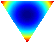
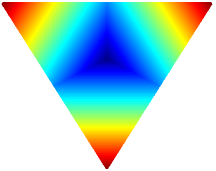
Figure 1: Contours of $\beta\mapsto\lVert\beta\rVert_{2}^{2}$ (left) and $\beta\mapsto\lVert\beta\rVert_{\infty}$ (right) on $\Delta^{3}$.

From the above discussion, we conclude that finding points of large $\ell_{2}$-norm is a reasonable surrogate for finding sparse solutions. This makes us propose the following modifications of $\widehat{\beta}$ and $\widetilde{\beta}_{\lambda}$, respectively.

$$\widehat{\beta}_{\lambda}^{\ell_{2}}\in\operatorname*{argmin}_{\beta\in\Delta^{p}}R_{n}(\beta)-\lambda\lVert\beta\rVert_{2}^{2},$$ (11)

$$\widetilde{\beta}_{\lambda}^{\ell_{2}}\in\operatorname*{argmin}_{\beta\in\mathcal{D}(\lambda)}-\lVert\beta\rVert_{2}^{2},\;\;\text{with $\mathcal{D}(\lambda)$ as in \eqref{eq:fcs}}$$ (12)

Note the correspondence of (11) / (12) on the one hand, and the lasso respectively Dantzig selector on the other hand.

Regarding (11), it appears more consequent to use $1/\lVert\beta\rVert_{2}^{2}$ in place of $-\lVert\beta\rVert_{2}^{2}$ in light of (10). Eventually, this is a matter of parameterization. While $\beta\mapsto\lVert\beta\rVert_{0}$ is the canonical measure of sparsity, $\beta\mapsto-1/\lVert\beta\rVert_{0}$ is another one. It is lower bounded by $\beta\mapsto-\lVert\beta\rVert_{2}^{2}$. We prefer the negative over the inverse for computational reasons: the optimization problem in (11) is a “difference of convex” (DC) program (Pham Dinh and Le Thi, 1997) and hence more amenable to optimization; see the next subsection for details.

The problem in (12) is also a DC program if $\mathcal{D}(\lambda)$ is convex. Note that for (12) minimizing the negative $\ell_{2}$-norm is equivalent to minimizing the inverse $\ell_{2}$-norm.

4.2 Least squares denoising

In order to show that the negative $\ell_{2}$-norm, when combined with simplex constraints, promotes exactly sparse solutions, we elaborate on (11) in the simple setup of denoising. Let $Z_{i}=\beta_{i}^{*}+\varepsilon_{i}$, $i=1,\ldots,n=p$, where $\beta^{*}\in\Delta_{0}^{n}(s)$ and the $\{\varepsilon_{i}\}_{i=1}^{n}$ represent random noise. We consider squared loss, i.e., $L(\beta,Z_{i})=(Z_{i}-\beta)^{2}$, $i=1,\ldots,n$. This yields the optimization problem

$$\vspace{-1ex}\min_{\beta\in\Delta^{n}}\frac{1}{n}\lVert\mathbf{Z}-\beta\rVert_{2}^{2}-\lambda\lVert\beta\rVert_{2}^{2},\;\;\mathbf{Z}=(Z_{i})_{i=1}^{n}.$$ (13)

It turns out that (13) can be recast as Euclidean projection of $\mathbf{Z}/\gamma$ on $\Delta^{n}$, where $\gamma$ is a function of $\lambda$. Based on this re-formulation, one can derive conditions on $\beta^{*}$ and $\lambda$ such that $\widehat{\beta}_{\lambda}^{\ell_{2}}$ achieves support recovery.

Proposition 3.

Consider (13) and suppose that $z_{(1)}>\ldots>z_{(n)}$, where the $\{z_{(i)}\}_{i=1}^{n}$ denote the ordered realizations of the $\{Z_{i}\}_{i=1}^{n}$. For all $\lambda\geq 1/n$, we have $\widehat{\beta}_{\lambda}^{\ell_{2}}=\big{(}\mathbf{I}(Z_{i}=z_{(1)})\big{)}_{i=1}^{n}$. For all $0\leq\lambda<1/n$, we have $\widehat{\beta}_{\lambda}^{\ell_{2}}=\operatorname*{argmin}_{\beta\in\Delta^{n}}\lVert\mathbf{Z}/\gamma-\beta\rVert_{2}^{2}$, where $\gamma=1-n\lambda$. Moreover, if $2s\max_{1\leq i\leq n}|\varepsilon_{i}|/n<\lambda<1/n$ and $b_{\min}^{*}>(n\lambda)/s+2\max_{1\leq i\leq n}|\varepsilon_{i}|$, we have $S(\widehat{\beta}_{\lambda}^{\ell_{2}})=S(\beta^{*})$.

In particular, for $\lambda=(1+\delta)2s\max_{1\leq i\leq n}|\varepsilon_{i}|/n$ for any $\delta>0$, the required lower bound on $b_{\min}^{*}$ becomes $4(1+\delta)\max_{1\leq i\leq n}|\varepsilon_{i}|$. For the sake of reference, we note that in the Gaussian sequence model with $\varepsilon_{i}\sim N(0,\sigma^{2}/n)$ (cf. Johnstone (2013)), we have $\max_{1\leq i\leq n}|\varepsilon_{i}|\asymp\sqrt{\log(n)/n}$.

The denoising problem (13) can be seen as least squares regression problem in which the design matrix equals the identity. For general design matrices, analysis becomes harder, in particular because the optimization problem may be neither convex nor concave. In the latter case, the minimum is attained at one of the vertices of $\Delta^{p}$.

4.3 Optimization

Both (11) and (12) are non-convex in general. Even more, maximizing the Euclidean norm over a convex set is NP-hard in general (Pardalos and Vavasis, 1991). To get a handle on these two problems, we exploit the fact that both objectives are in DC form, i.e., can be represented as $f(\beta)=g(\beta)-h(\beta)$ with $g$ and $h$ both being convex. Linearizing $-h$ at a given point yields a convex majorant of $f$ that is tight at that point. Minimizing the majorant and repeating yields an iterative procedure known as concave-convex procedure (CCCP, Yuille and Rangarajan (2003)) that falls into the more general framework of majorization-minimization (MM) algorithms (Lange et al., 2000). When applied to (11) and (12), this approach yields Algorithm 1.

Algorithm 1

(11): $\min_{\beta\in\Delta^{p}}R_{n}(\beta)-\lambda\lVert\beta\rVert_{2}^{2}$

  Initialization: $\beta^{0}\in\Delta^{p}$

  repeat $\;\beta^{k+1}\in\operatorname*{argmin}_{\beta\in\Delta^{p}}R_{n}(\beta)-2\left\langle\beta^{k},\beta-\beta^{k}\right\rangle$

  until $\;\;\,R_{n}(\beta^{k+1})-2\left\langle\beta^{k},\beta^{k+1}\right\rangle=R_{n}(\beta^{k})$

  (12): $\min_{\beta\in\mathcal{D}(\lambda)}-\lVert\beta\rVert_{2}^{2}$

  Initialization: $\beta^{0}\in\mathcal{D}(\lambda)$

  repeat $\beta^{k+1}\in\operatorname*{argmin}_{\beta\in\mathcal{D}(\lambda)}-2\left\langle\beta^{k},\beta-\beta^{k}\right\rangle$

  until $\left\langle\beta^{k},\beta^{k+1}-\beta^{k}\right\rangle=0$

For the second part of Algorithm 1 to be practical, it is assumed that $\mathcal{D}(\lambda)$ is convex. The above algorithms can be shown to yield strict descent until convergence to a limit point satisfying the first-order optimality condition of the problems (11)/(12). This is the content of the next proposition.

Proposition 4.

Let $f$ denote the objective in (11) or (12). The elements of the sequence $\{\beta^{k}\}_{k\geq 0}$ produced by the above algorithms are feasible for problems (11) resp. (12) and satisfy $f(\beta^{k+1})<f(\beta^{k})$ until convergence. Moreover, the limit satisfies the first-order optimality condition of the respective problem.

An appealing feature of Algorithm 1 is that solving each sub-problem in the repeat step only involves minor modifications of the computational approaches used for ERM resp. finding a feasible point in $\mathcal{D}(\lambda)$.

When selecting the parameter $\lambda$ by means of a grid search, we suggest solving the associated instances of (11)/(12) from the smallest to the largest value of $\lambda$, using the solution from the current instance as initial iterate for the next one. For the smallest value of $\lambda$, we recommend using $\widehat{\beta}$ and any point from $\mathcal{D}(\lambda)$ as initial iterate for (11) respectively (12). Running Algorithm 1 for formulation (12) has the advantage that all iterates are contained in $\mathcal{D}(\lambda)$ and thus enjoy at least the statistical guarantees of $\widetilde{\beta}_{\lambda}$ derived in $\S$2. According to our numerical results, it is formulation (11) that achieves better performance (cf. $\S$6).

4.4 Comparison to other regularization schemes

There exist a variety of other regularization schemes one may want to consider for the given problem, in particular those already mentioned in the introduction. The present subsection provides a more detailed overview on such alternatives, and we justify why we think that our proposal offers advantages.

Iterative Hard Thresholding (Kyrillidis et al., 2013).      This is an iterative algorithm whose iterates are given by the relation

$$\beta^{k+1}\leftarrow\Pi_{\Delta_{0}^{p}(s)}(\beta^{k}-\alpha^{k}\nabla R_{n}(\beta^{k})),$$

where the projection operator $\Pi_{\Delta_{0}^{p}(s)}$ can be evaluated in near-linear time (Kyrillidis et al., 2013). As pointed out above, $s$ is typically not known. Numerical results suggest that the approach is sensitive to over-specification of $s$ (cf. ). A second issue is the choice of the step-sizes $\{\alpha^{k}\}$. Kyrillidis et al. (2013) consider a constant step-size based on the Lipschitz constant of the gradient as normally used for projected gradient descent with convex constraint sets (Bertsekas, 1999), as well as strategy developed in Kyrillidis and Cevher (2011). Neither of these has been supported by theoretical analysis. For squared loss, convergence guarantees can be established under the restricted isometry property (RIP) and a constant step-size depending on RIP constants, which are not accessible in practice.

Inverse $\ell_{\infty}$-regularization (Pilanci et al., 2012).      Pilanci et al. (2012) consider regularized risk estimation with the inverse of the $\ell_{\infty}$-norm as regularizer, that is

$$\operatorname*{argmin}_{\beta\in\Delta^{p}}R_{n}(\beta)+\lambda(1/\lVert\beta\rVert_{\infty}).$$ (14)

As discussed above and illustrated by Figure 1, the function $\beta\mapsto 1/\lVert\beta\rVert_{\infty}$ is sparsity-promoting on $\Delta^{p}$. While this function is non-convex, problem (14) can be reduced to $p$ convex optimization problems (one for each coordinate, Pilanci et al. (2012)). This is an appealing property, but the computational effort that is required to solve these $p$ convex optimization problem is out of proportion compared to most other approaches considered herein. In noiseless settings, computation is more manageable since $\lambda$ does not need to be tuned. In our numerical studies, the performance is inferior to (11)/(12).

Entropy regularization (Shashanka et al., 2008).      For $\beta\in\Delta^{p}$, consider the Shannon entropy $\beta\mapsto\mathcal{H}(\beta)\mathrel{\mathop{:}}=-\sum_{j=1}^{p}\log(\beta_{j})\beta_{j}$ with the convention $\log(0)\cdot 0=0$. While $\mathcal{H}$ is a natural measure of sparsity on $\Delta^{p}$, there is a computational issue that makes it less attractive. It is not hard to show that the subdifferential (Rockafellar, 1970) of $\mathcal{H}$ is empty at any point in $\partial\Delta^{p}\mathrel{\mathop{:}}=\{x\in\Delta^{p}:\,\exists j\;\text{s.t.}\;x_{j}=0\}$. Because of this, approaches that make use of (sub-)gradients of the regularizer such as projected (sub-)gradient descent or DC programming) cannot be employed. As already mentioned, coordinate descent is not an option given the simplex constraints. A workaround would be the use of $\mathcal{H}_{\varepsilon}(\beta)=-\sum_{j=1}^{p}\log(\beta_{j}+\varepsilon)\beta_{j}$ for some $\varepsilon>0$. This leads to an extra parameter in addition to the regularization parameter, which we consider as a serious drawback. In fact, $\varepsilon$ needs to be tuned as values very close to zero may negatively affect convergence of iterative algorithms used for optimization.

$\ell_{q}$-regularization for $0<q<1$.      The regularizer $\beta\mapsto\lVert\beta\rVert_{q}^{q}=\sum_{j=1}^{p}\beta_{j}^{q}$ for $\beta\in{\mathbb{R}}_{+}^{p}$suffers from the same issue as the entropy regularizer: the subdifferential is empty for all points in $\partial\Delta^{p}$. Apart from that, it is not clear how close $q$ needs to be to zero so that appropriately sparse solutions are obtained.

Log-sum regularization (Candes et al., 2007; Larsson and Ugander, 2011).      The regularizer $\beta\mapsto\sum_{j=1}^{p}\log(\beta_{j}+\varepsilon)$ for $\beta\in{\mathbb{R}}_{+}^{p}$ and $\varepsilon>0$ is suggested in Candes et al. (2007). When restricted to $\Delta^{p}$, the above regularizer can be motivated from a Bayesian viewpoint as in terms of a specific prior on $\beta$ called pseudo-Dirichlet in Larsson and Ugander (2011). The above regularizer is concave and continuously differentiable and can hence be tackled numerically via DC programming in the same manner as in Algorithm 1. Again, the choice of $\varepsilon$ may have a significant effect on the result/convergence and thus needs to be done with care. Small values of $\varepsilon$ lead to a close approximation of the $\ell_{0}$-norm. While this is desired in principle, optimization (e.g. via Algorithm 1) becomes more challenging as the regularizer approaches discontinuity at zero.

Minimax concave penalty (Zhang, 2010) and related regularizers.      The minimax concave penalty (MCP) can be written as $P(\beta)=\lambda\lVert\beta\rVert_{1}+Q(\beta)$ with

$$Q(\beta)=\sum_{j=1}^{p}\left\{-\frac{\beta_{j}^{2}}{2b}\textbf{I}(|\beta_{j}|\leq b\lambda)+\left(\frac{b\lambda^{2}}{2}-\lambda|\beta_{j}|\right)\textbf{I}(|\beta_{j}|>b\lambda)\right\},$$

where $\lambda,b>0$ are parameters. Since $\lVert\beta\rVert_{1}=1\,\forall\beta\in\Delta^{p}$, the MCP reduces to $Q$ under simplex constraints. Using the re-parameterization $(\lambda,b)\mapsto(\lambda,\theta\mathrel{\mathop{:}}=b\lambda)$, we have

$$Q(\beta)=\sum_{j=1}^{p}\left\{-\frac{\lambda}{2\theta}\beta_{j}^{2}\textbf{I}(|\beta_{j}|\leq\theta)+\left(\frac{\lambda\theta}{2}-\lambda\beta_{j})\textbf{I}(|\beta_{j}|>\theta\right)\right\}$$

Under simplex constraints, $\theta$ can be restricted to $(0,1]$. Note that for $\theta=1$, $Q(\beta)=-(\lambda/2)\lVert\beta\rVert_{2}^{2}$, in which case the MCP boils down to the negative $\ell_{2}$-regularizer suggested in the present work. On the other hand, as $\theta\rightarrow 0$, the MCP behaves like the $\ell_{0}$-norm. The MCP is concave and continuously differentiable so that the approach of Algorithm 1 can be applied. Clearly, by optimizing the choice of the parameter $\theta$, MCP has the potential to improve over the negative $\ell_{2}$-regularizer in (11), which results as special case for $\theta=1$. Substantial improvement is not guaranteed though and entails additional effort for tuning $\theta$.

The SCAD (Fan and Li, 2001) and capped $\ell_{1}$-regularization (Zhang and Zhang, 2013) follow a design principle similar to that of MCP. All three are coordinate-wise separable and resemble the $\ell_{1}$-norm for values close to zero and flatten out for larger values so as to serve as better proxy of the $\ell_{0}$-norm than the $\ell_{1}$-norm. A parameter (like $\theta$ for MCP) controls what exactly is meant by “close to zero” respectively “large”. Note the conceptual difference between this class of regularizers and negative $\ell_{2}$-regularization: members of the former have been designed as concave approximations to the $\ell_{0}$-norm at the level of a single coordinate, whereas the latter has been motivated as a proxy for the $\ell_{0}$-norm on the simplex.

Convex envelope (Jojic et al., 2011).      An approach completely different from those discussed so far can be found in Jojic et al. (2011). A common way of motivating $\ell_{1}$-regularization is that the $\ell_{1}$-norm is the convex envelope (also known as bi-conjugate, Rockafellar (1970)), i.e., the tightest convex minorant, of the $\ell_{0}$-norm on the unit $\ell_{\infty}$-ball. Instead of using the convex envelope of only the regularizer, Jojic et al. (2011) suggest that one may also use convex envelope of the entire regularized risk $R_{n}(\beta)+\lambda\lVert\beta\rVert_{0}$. The authors argue that this approach is suitable for promoting sparsity under simplex constraints. Moreover, the resulting optimization problem is convex so that computing a global optimum appears to be feasible. However, it is in general not possible to derive a closed form expression for the convex envelope of the entire regularized risk. In this case, alreay evaluating the convex envelope at a single point requires solving a convex optimization problem via an iterative algorithm. It is thus not clear whether there exist efficient algorithms for minimizing the resulting convex envelope.

5 Extension to the matrix case

As pointed out in the introduction, there is a matrix counterpart to the problem discussed in the previous settings in which the object of interest is a low-rank Hermitian positive semidefinite matrix of unit trace. This set of matrices covers density matrices of quantum systems (Nielsen and Chuang, 2000). The task of reconstructing such density matrices from so-called observables (as e.g. noisy linear measurements) is termed quantum state tomography (Paris and Rehacek, 2004). In the past few years, quantum state tomography based on Pauli measurements has attracted considerable interest in mathematical signal processing and statistics (Gross et al., 2010; Gross, 2011; Koltchinskii, 2011; Wang, 2013; Cai et al., 2016).

Specifically, the setup that we have in mind throughout this section is as follows. Let ${\mathbb{H}}^{m}=\{B\in{\mathbb{C}}^{m\times m}:B=B^{H}\}$ be the Hilbert space of complex Hermitian matrices with innner product $\left\langle F,G\right\rangle=\operatorname*{tr}(FG)$, $(F,G)\in{\mathbb{H}}\times{\mathbb{H}}$, and let henceforth $\lVert\cdot\rVert_{q}$, $0\leq q\leq\infty$, denote the Schatten $q$-’norm’ of a Hermitian matrix, defined as the $\ell_{q}$-norm of its eigenvalues. In particular, $\lVert\cdot\rVert_{0}$ denotes the number of non-zero eigenvalues, or equivalently, the rank. We suppose that the target $B^{*}$ is contained in the set $\bm{\Delta}_{0}^{m}(r)\mathrel{\mathop{:}}=\bm{B}_{0}^{m}(r)\cap\bm{\Delta}^{m}$, where

$$\bm{B}_{0}^{m}(r)\mathrel{\mathop{:}}=\{B\in{\mathbb{H}}^{m}:\;\lVert B\rVert_{0}\leq r\},\quad\;\,\text{and}\;\;\bm{\Delta}^{m}\mathrel{\mathop{:}}=\{B\in{\mathbb{H}}^{m}:B\succeq 0,\,\operatorname*{tr}(B)=1\}.$$

i.e., $B^{*}$ is additionally positive semidefinite, of unit trace and has rank at most $r$. In low-rank matrix recovery, the Schatten 1-norm (typically referred to as the nuclear norm) is commonly used as convex surrogate for the rank of a matrix (Recht et al., 2010). Since the nuclear norm is constant over $\bm{\Delta}^{m}$, one needs a different strategy to promote low-rankendess under that constraint. In the sequel, we carry over our treatment of the vector case to the matrix case. The analogies are rather direct; at certain points, however, an extension to the matrix case may yield additional complications as detailed below. To keep matters simple, we restrict ourselves to the setup in which the $Z_{i}=(X_{i},Y_{i})$ are such that

$$\vspace{-1ex}Y_{i}=\left\langle X_{i},B^{*}\right\rangle+\varepsilon_{i},\;\;\varepsilon_{i}\sim N(0,\sigma^{2}),\;i=1,\ldots,n,$$ (15)

with $\{X_{i}\}_{i=1}^{n}\subset{\mathbb{H}}^{m}$. Equivalently,

$$\mathbf{Y}=\mathcal{X}(B^{*})+\varepsilon,\;\;\mathbf{Y}=(Y_{i})_{i=1}^{n},\;\varepsilon=(\varepsilon_{i})_{i=1}^{n},$$

where $\mathcal{X}:{\mathbb{H}}^{m}\rightarrow{\mathbb{R}}^{n}$ is a linear operator defined by $(\mathcal{X}(B))_{i}=\left\langle X_{i},B\right\rangle$, $B\in{\mathbb{H}}^{m}$, $i=1,\ldots,n$. We consider squared loss, i.e., for $B\in\bm{\Delta}^{m}$ the empirical risk reads

$$\vspace{-1ex}R_{n}(B)=\lVert\mathbf{Y}-\mathcal{X}(B)\rVert_{2}^{2}/n.$$

Basic estimators.

As basic estimators, we consider empirical risk minimization given by $\widehat{B}\in\operatorname*{argmin}_{B\in\bm{\Delta}^{m}}R_{n}(B)$, as well as $\widetilde{B}_{\lambda}$, where $\widetilde{B}_{\lambda}$ is any point in the set

$$\bm{D}(\lambda)=\{B\in\bm{\Delta}^{m}:\lVert\nabla R_{n}(B)\rVert_{\infty}\leq\lambda\}=\Big{\{}B\in\bm{\Delta}^{m}:\frac{2}{n}\lVert\mathcal{X}^{\star}(\mathcal{X}(B)-y)\rVert_{\infty}\leq\lambda\Big{\}},$$ (16)

where $\mathcal{X}^{\star}:{\mathbb{R}}^{n}\rightarrow{\mathbb{H}}^{m}$ is the adjoint of $\mathcal{X}$. Both $\widehat{B}$ and $\widetilde{B}_{\lambda}$ show adaptation to the rank of $B^{*}$ under the following restricted strong convexity condition. For $B\in\bm{B}_{0}^{m}(r)\subset{\mathbb{H}}^{m}$, let ${\mathbb{T}}(B)$ be the tangent space of $\bm{B}_{0}^{m}(r)\subset{\mathbb{H}}^{m}$ at $B$ (see Definition E.1 in the appendix). and let $\Pi_{V}$ denote the projection on a subspace $V$ of ${\mathbb{H}}^{m}$.

Condition 2.

We say that the $\bm{\Delta}$-RSC condition is satified for rank $r$ and constant $\kappa>0$ if $\forall\Phi\in\mathcal{K}^{\bm{\Delta}}(r)$ $\lVert\mathcal{X}(\Phi)\rVert_{2}^{2}/n\geq\kappa\lVert\Phi\rVert_{2}^{2}$, where

$$\mathcal{K}^{\bm{\Delta}}(r)=\{\Phi\in\mathbb{H}^{m}:\,\exists B\in\bm{B}_{0}^{m}(r)\,\text{s.t.}$$

$$\operatorname*{tr}(\Pi_{\mathbb{T}(B)^{\perp}}(\Phi))=-\operatorname*{tr}(\Pi_{\mathbb{T}(B)}\Phi)\;\text{and}\;\Pi_{\mathbb{T}(B)^{\perp}}(\Phi)\succeq 0\}.$$

The $\bm{\Delta}$-RSC condition is weaker than the corresponding condition employed in Negahban and Wainwright (2011), which in turn is weaker than the matrix RIP condition Recht et al. (2010). The next statement parallels Proposition 2, asserting that the constraint $B\in\bm{\Delta}^{m}$ alone is strong enough to take advantage of low-rankedness.

Proposition 5.

Suppose that the $\bm{\Delta}$-RSC condition is satisfied for rank $r$ and $\kappa>0$. Set $\lambda_{*}=2\lVert\mathcal{X}^{\star}(\varepsilon)\rVert_{\infty}/n$, where $\mathcal{X}^{\star}:{\mathbb{R}}^{n}\rightarrow{\mathbb{H}}^{m}$ is the adjoint of $\mathcal{X}$. We then have

$$\lVert\widehat{B}-B^{*}\rVert_{2}^{2}\leq\frac{4s\lambda_{*}^{2}}{\kappa^{2}},\quad\lVert\widetilde{B}_{\lambda}-B^{*}\rVert_{2}^{2}\leq\frac{4s(\lambda+\lambda_{*})^{2}}{\kappa^{2}},$$

$$\lVert\widehat{B}-B^{*}\rVert_{1}\leq\frac{4s\lambda_{*}}{\kappa},\quad\lVert\widetilde{B}_{\lambda}-B^{*}\rVert_{1}\leq\frac{4s(\lambda+\lambda_{*})}{\kappa}.$$

Obtaining solutions of low rank.

While $\widehat{B}$ may have low estimation error its rank can by far exceed the rank of $B^{*}$, even though the extra non-zero eigenvalues of $\widehat{B}$ may be small. The simplest approach to obtain solutions of low rank is to apply thresholding to the spectrum of $\widehat{B}=\widehat{U}\widehat{\Phi}\widehat{U}^{\top}$ (the r.h.s. representing the usual spectral decomposition), that is $\widehat{B}_{\tau}=\widehat{U}\widehat{\Phi}_{\tau}\widehat{U}^{\top}$, where $\widehat{\Phi}_{\tau}=\text{diag}(\{\mathbf{I}(\widehat{\phi}_{j}\geq\tau)\}_{j=1}^{m})$ for a threshold $\tau>0$. Likewise, one may consider the following analog to weighted $\ell_{1}$-regularization:

$$\begin{split}&\widehat{B}_{w}=\widehat{U}\text{diag}(\{\widehat{\phi}_{w,j}\}_{j=1}^{m})\widehat{U}^{\top},\\ \text{where}\;\,&\widehat{\phi}_{w}\in\operatorname*{argmin}_{\phi\in\Delta^{p}}\frac{1}{n}\lVert\mathbf{Y}-\mathcal{X}(\widehat{U}\text{diag}(\{\phi_{j}\}_{j=1}^{m})\widehat{U}^{\top})\rVert_{2}^{2}+\lambda\left\langle w,\phi\right\rangle\end{split}$$ (17)

for non-negative weights $\{w_{j}\}_{j=1}^{m}$ as in the vector case. Note that the matrix of eigenvectors $\widehat{U}$ is kept fixed at the second stage; the optimization is only over the eigenvalues. Alternatively, one may think of optimization over $\bm{\Delta}^{m}$ with regularizer $B\mapsto\lVert B\rVert_{w}=\sum_{j=1}^{m}w_{j}\phi_{j}(B)$ for eigenvalues $\phi_{1}(B)\geq\ldots\geq\phi_{m}(B)\geq 0$ of $B$ in decreasing order. However, from the point of view of optimization $\lVert\cdot\rVert_{w}$ poses difficulties, possible non-convexity (depending on $w$) in particular.

Regularization with the negative $\ell_{2}$-norm.

One more positive aspect about the regularization scheme proposed in $\S$4 is that it allows a straightforward extension to the matrix case, including the algorithm used for optimization (Algorithm 1). By contrast, for regularization with the inverse $\ell_{\infty}$-norm, which can be reduced to $p$ convex optimization problems in the vector case, no such reduction seems to be possible in the matrix case. The analogs of (11)/(12) are given by

$$\widehat{B}_{\lambda}^{\ell_{2}}\in\operatorname*{argmin}_{B\in\bm{\Delta}^{m}}R_{n}(\beta)-\lambda\lVert B\rVert_{2}^{2},$$ (18)

$$\widetilde{B}_{\lambda}^{\ell_{2}}\in\operatorname*{argmin}_{B\in\bm{D}(\lambda)}-\lVert B\rVert_{2}^{2}.$$ (19)

Algorithm 1 can be employed for optimization mutatis mutandis. In the vector case and for squared loss, formulations (11) and (12)are comparable in terms of computational effort: each minimization problem inside the ’repeat’-loop becomes a quadratic respectively a linear program with a comparable number of variables/constraints. In the matrix case, however, (18) appears to be preferable as the sub-problems are directly amenable to a proximal gradient method. By contrast, the constraint set in (19) requires a more sophisticated approach.

Denoising.

Negative $\ell_{2}$-regularization in combination with the constraint set $\bm{\Delta}^{m}$ enforces solution of low rank as exemplified here in the special case of denoising of a real-valued matrix (i.e., $B^{*}\in{\mathbb{H}}^{m}\cap{\mathbb{R}}^{m\times m}$) contaminated by Gaussian noise. Specifically, the sampling operator $\mathcal{X}(\cdot)=(\left\langle X_{i},\cdot\right\rangle)_{i=1}^{n}$, $n=m(m+1)/2$, here equals the symmetric vectorization operator, that is

$$\begin{split}&X_{1}=e_{1}e_{1}^{\top},\;\;X_{2}=\frac{e_{1}e_{2}^{\top}+e_{2}e_{1}^{\top}}{\sqrt{2}},\ldots,X_{m}=\frac{e_{1}e_{m}^{\top}+e_{m}e_{1}^{\top}}{\sqrt{2}},\;\;X_{m+1}=e_{2}e_{2}^{\top},\ldots,\\ &X_{2m-1}=\frac{e_{2}e_{m}^{\top}+e_{m}e_{2}^{\top}}{\sqrt{2}},\ldots,X_{m(m+1)/2}=\frac{e_{m-1}e_{m}^{\top}+e_{m}e_{m-1}^{\top}}{\sqrt{2}}\end{split}$$ (20)

The following proposition makes use of a result in random matrix theory due to Peng (2012).

Proposition 6.

Let $B^{*}\in\bm{\Delta}_{0}^{m}(r)\cap{\mathbb{R}}^{m\times m}$ with eigenvalues $\phi_{1}^{*}\geq\ldots\geq\phi_{r}^{*}>0$ and $\phi_{r+1}^{*}=\ldots=\phi_{m}^{*}=0$, let $\mathcal{X}$ be defined according to (20), and let futher $\varepsilon\sim N(0,\sigma^{2}I_{m}/m)$, $\mathbf{Y}=\mathcal{X}(B^{*})+\varepsilon$. Consider the optimization problem

$$\min_{B\in\bm{\Delta}^{m}}\frac{1}{n}\lVert\mathbf{Y}-\mathcal{X}(B)\rVert_{2}^{2}-\lambda\lVert B\rVert_{2}^{2}$$

with minimizer $\widehat{B}_{\lambda}^{\ell_{2}}$ and define $\Upsilon=B^{*}+\mathcal{X}^{\star}(\varepsilon)$. Then, for all $\lambda\geq 1/n$, we have $\widehat{B}_{\lambda}^{\ell_{2}}=u_{1}u_{1}^{\top}$, where $u_{1}$ is the eigenvector of $\Upsilon$ corresponding to its largest eigenvalue. For all $0\leq\lambda<1/n$, we have $\widehat{B}_{\lambda}^{\ell_{2}}=\operatorname*{argmin}_{B\in\bm{\Delta}^{m}}\lVert\Upsilon/\gamma-B\rVert_{2}^{2}$, where $\gamma=1-n\lambda$. Moreover, there exists constants $c_{0},c,C>0$ so that if $r<c_{0}m$, $\lambda\geq 6\sigma r/n$ and $\phi_{r}^{*}\geq 5\sigma+n\lambda/r$, we have $\lVert\widehat{B}_{\lambda}^{\ell_{2}}\rVert_{0}=r$ with probability at least $1-C\exp(-cm)$.

In particular, for $\lambda=(1+\delta)6\sigma r/n$ for some $\delta>0$, the required lower bound on $\phi_{r}^{*}$ becomes $11(1+\delta)\sigma$, which is proportional to the noise level of the problem as follows from the proof of the proposition.

Alternative regularization schemes.

The approaches of $\S$4.4 can in principle all be extended to the matrix case by defining corresponding regularizers in terms of the spectrum of a positive semidefinite matrix. For example, the Shannon entropy becomes the von Neumann entropy (Nielsen and Chuang, 2000). It is important to note that in Koltchinskii (2011), the negative of the von Neumann entropy is employed, without constraining the target to be contained in $\bm{\Delta}^{m}$. The negative von Neumann entropy still ensures positive semidefiniteness and boundedness of the solution. Schatten $\ell_{q}$-regularization with $0<q<1$ for low rank matrix recovery is discussed in Mohan and Fazel (2012); Rohde and Tsybakov (2011). In a recent paper, Gui and Gu (2015) analyze statistical properties of the counterparts of MCP and SCAD in the matrix case. For details, we refer to the cited references and the references therein; our reasoning for prefering negative $\ell_{2}$-regularization persists.

6 Empirical results

We have conducted a series of simulations to compare the different methods considered herein and to provide additional support for several key aspects of the present work. Specifically, we study compressed sensing, least squares regression, mixture density estimation, and quantum state tomography based on Pauli measurements in the matrix case. The first two of these only differ by the presence respectively absence of noise. We also present a real data analysis example concerning portfolio optimization for NASDAQ stocks based on weekly price data from 03/2003 to 04/2008.

6.1 Compressed sensing

We consider the problem of recovering $\beta^{*}\in\Delta_{0}^{p}(s)$ from a small number of random linear measurements $Y_{i}=\left\langle X_{i},\beta^{*}\right\rangle$, where $X_{i}$ is standard Gaussian, $i=1,\ldots,n$. In short, $\mathbf{Y}=\bm{X}\beta^{*}$ with $\mathbf{Y}=(Y_{i})_{i=1}^{n}$ and $\bm{X}$ having the $\{X_{i}\}_{i=1}^{n}$ as its rows. Identifying $\beta^{*}$ with a probability distribution $\pi$ on $\{1,\ldots,p\}$, we may think of the problem as recovering such distribution from expectations of the form $Y_{i}=\sum_{j=1}^{p}(X_{i})_{j}\pi(\{j\})$. We here show the results for $p=500$, $s=50$ and $n=cs\log(p/s)$ with $c\in[0.8,2]$ (cf. Figure 2). The target $\beta^{*}$ is generated by selecting its support uniformly at random, drawing the non-zero entries randomly from $[0,1]$ and normalizing subsequently. This is replicated $50$ times for each value of $n$.

The following approaches are compared for the given task, assuming squared loss $R_{n}(\beta)=\lVert\mathbf{Y}-\bm{X}\beta\rVert_{2}^{2}/n$.

’Feasible set’: Note that ERM here amounts to finding a point in $\mathcal{D}(0)$. The output is used as initial iterate for ’L2’, ’weighted L1’, and ’IHT’ below.
’L2’: $\ell_{2}$-norm maximization (12) with $\lambda=0$, i.e., over

$$\begin{split}\mathcal{D}(0)&=\{\beta\in\Delta^{p}:\;\bm{X}^{\top}(\bm{X}\beta-\mathbf{Y})=0\}\\ &=\{\beta\in\Delta^{p}:\;\bm{X}\beta=\mathbf{Y}\}\;\;\text{with probability 1}.\end{split}$$ (21)

’Pilanci’: The method of Pilanci et al. (2012) that maximizes the $\ell_{\infty}$-norm over (21).

’weighted L1’: Weighted $\ell_{1}$-norm minimization (cf. $\S$3) over (21).

’IHT’: Iterative hard threshold under simplex constraints (Kyrillidis et al., 2013). Regarding the step size used for gradient projection, we use the method in Kyrillidis and Cevher (2011) which empirically turned out to be superior compared to a constant step size. ’IHT’ is run with the correct value of $s$ and is hence given an advantage.

Results.    Figure 2 visualizes the fractions of recovery out of $50$ replications. A general observation is that the constraint $\beta\in\Delta^{p}$ is powerful enough to reduce the required number of measurements considerably compared to $2s\log(p/s)$ when using standard $\ell_{1}$-minimization without constraints. At this point, we refer to Donoho and Tanner (2005) who gave a precise asymptotic characterization of this phenomenon in a “proportional growth” regime, i.e., $n/p\rightarrow c\in(0,1)$ and $s/n\rightarrow c^{\prime}\in(0,1)$. When solving the feasibility problem, one does not explicitly exploit sparsity of the solution (even though the constraint implicitly does). Enforcing sparsity via ’Pilanci’, ’IHT’, ’L2’ further improves performance. The improvements achieved by ’L2’ are most substantial and persist throughout all sparsity levels. ’weighted L1’ does not consistenly improve over the solution of the feasibility problem.

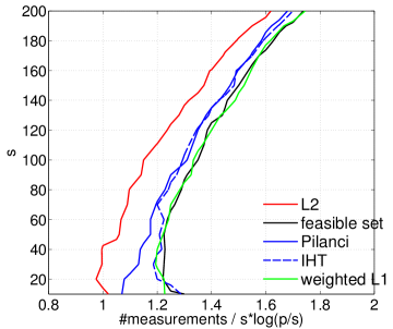
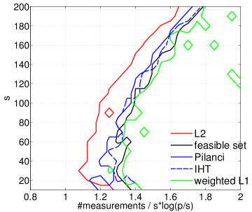
Figure 2: Contour plots of the empirical relative frequencies of exact recovery in dependency of the number of measurements (horizontal axis) and $s$ (vertical axis). The left and right plot show the contour levels $.75$ and $.99$, respectively. Note that the smaller the area “left” to and “above” the curve, the better the performance.

6.2 Least squares regression

We next consider the Gaussian linear regression model (8) with the $\{X_{i}\}_{i=1}^{n}$ as in the previous subsection. Put differently, the previous data-generating model is changed by an additive noise component. The target $\beta^{*}$ is generated as before, with the change that the subvector $\beta_{S(\beta^{*})}^{*}$ corresponding to $S(\beta^{*})$ is projected on $[b_{\min}^{*},1]^{s}\cap\Delta^{s}$ to ensure sufficiently strong signal, where $b_{\min}^{*}=\varrho\sigma\sqrt{2\log(p)/n}$ with $\sigma=s^{-1}$ and $\varrho=1.7$ controlling the signal strength relative to the noise level $\lambda_{0}=\sigma\sqrt{2\log(p)/n}$. The following approaches are compared.

’ERM’: Empirical risk minimization.

’Thres’: ’ERM’ followed by hard thresholding (cf. $\S$3).

’L2-ERM’: Regularized ERM with negative $\ell_{2}$-regularization (11). For the parameter $\lambda$, we consider a grid $\Lambda$ of 100 logarithmically spaced points from $0.01$ to $\phi_{\max}(\bm{X}^{\top}\bm{X}/n)$, the maximum eigenvalue of $\bm{X}^{\top}\bm{X}/n$. Note that for $\lambda\geq\phi_{\max}(\bm{X}^{\top}\bm{X}/n)$, the optimization problem (11) becomes concave and the minimizer must consequently be a vertex of $\Delta^{p}$, i.e., the solution is maximally sparse at this point, and it hence does not make sense to consider even larger values of $\lambda$. When computing the solutions $\{\widehat{\beta}_{\lambda}^{\ell_{2}},\,\lambda\in\Lambda\}$, we use a homotopy-type scheme in which for each $\lambda\in\Lambda$, Algorithm 1 is initialized with the solution for the previous $\lambda$, using the output $\widehat{\beta}$ of ’ERM’ as initialization for the smallest value of $\lambda$.

’L2-D’: $\ell_{2}$-norm maximization (12) over $\mathcal{D}(C\lambda_{0})$ with $\lambda_{0}$ being the noise level defined above and $C\in\{0.5,0.55,\ldots,2\}$. Algorithm 1 is initialized with $\widehat{\beta}$ provided it is feasible. Otherwise, a feasible point is computed by linear programming.
’weighted L1’: The approach in (6). Regarding the regularization parameter, we follow van de Geer et al. (2013) who let $\lambda=C\lambda_{0}^{2}$. We try 100 logarithmically spaced values between 0.1 and 10 for $C$.

’IHT’: As above, again with the correct value of $s$. We perform a second sets of experiments though in which $s$ is over-specified by different factors ($1.2$, $1.5$, $2$) in order to investigate the sensitivity of the method w.r.t. the choice of the sparsitity level.

’L1’: The approach (7), i.e., dropping the unit sum constraint and normalizing the output of the non-negative $\ell_{1}$-regularized estimator $\widehat{\beta}_{\lambda}^{\ell_{1}}$. We use $\lambda=\lambda_{0}$ as recommended in the literature, cf. e.g. Negahban et al. (2012).

’oracle’: ERM given knowledge of the support $S(\beta^{*})$.

For ’Thres’,’L2-ERM’ and other methods for which multiple values of a hyperparameter are considered, hyperparameter selection is done by minimizing the RIC as defined in $\S$3 after evaluating each support set returned for a specific value of the hyperparameter.

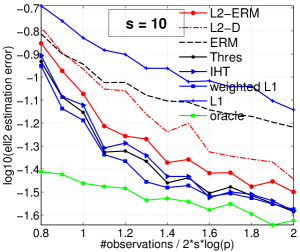
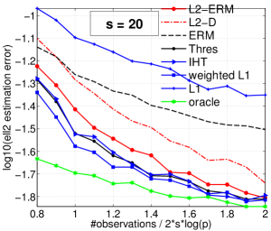
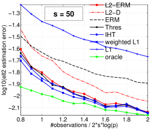
$\begin{array}[]{l}\text{{Standard errors}(rounded):}\\ \begin{array}[]{|c|c|c|c|}\hline\cr\textbf{{L2-ERM}}&\textbf{{L2-D}}&\textbf{{ERM}}&\textbf{{Thres}}\\ .04&.04&.02&0.04\\ \hline\cr\textbf{{weightedL1}}&\textbf{{IHT}}&\textbf{{L1}}&\textbf{{oracle}}\\ .04&.04&.02&.02\\ \hline\cr\end{array}\end{array}$	$\begin{array}[]{l}\text{{Standard errors}(rounded):}\\ \begin{array}[]{|c|c|c|c|}\hline\cr\textbf{{L2-ERM}}&\textbf{{L2-D}}&\textbf{{ERM}}&\textbf{{Thres}}\\ .03&.03&.01&0.03\\ \hline\cr\textbf{{weightedL1}}&\textbf{{IHT}}&\textbf{{L1}}&\textbf{{oracle}}\\ .03&.03&.01&.01\\ \hline\cr\end{array}\end{array}$	$\begin{array}[]{l}\text{{Standard errors}(rounded):}\\ \begin{array}[]{|c|c|c|c|}\hline\cr\textbf{{L2-ERM}}&\textbf{{L2-D}}&\textbf{{ERM}}&\textbf{{Thres}}\\ .02&.02&.01&0.02\\ \hline\cr\textbf{{weightedL1}}&\textbf{{IHT}}&\textbf{{L1}}&\textbf{{oracle}}\\ .02&.02&.01&.01\\ \hline\cr\end{array}\end{array}$

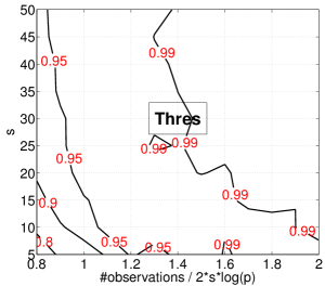
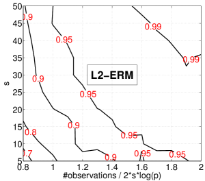
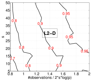
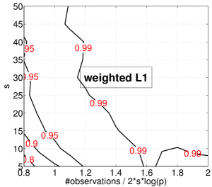
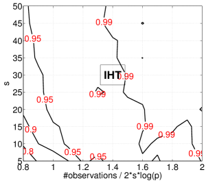
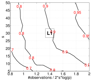
Figure 3: Upper panel: Average estimation errors $\lVert\widehat{\theta}-\beta^{*}\rVert_{2}$ ($\log_{10}$ scale) in dependence of $n$ over 50 trials for selected values of $s$. Here, $\widehat{\theta}$ is a placeholder for any of the the estimators under consideration. Middle and Lower panel: contour plots of the average Matthew’s correlation in dependence of $n$ (horizontal axis) and $s$ (vertical axis) for the contour levels $0.7,0.8,0.9,0.95$. Note that the smaller the area between the lower left corner of the plot and a contour line of a given level, the better the performance.

Results. The results are summarized in Figures 3 and 4. Turning to the upper panel of Figure 3, the first observation is that ’L1’ yields noticeably higher $\ell_{2}$ estimation errors than ’ERM’, which yields a reductions roughly between a factor of $10^{-.1}\approx 0.79$ and $10^{-.2}\approx 0.63$. A further reduction in error of about the same order is achieved by several of the above methods. Remarkably, the basic two-stage methods, thresholding and weighted $\ell_{1}$-regularization for the most part outperform the more sophisticated methods. Among the two methods based on negative $\ell_{2}$-regularization, ’L2-ERM’ achieves better performance than ’L2-D’. We also investigate sucess in support recovery by comparing $S(\widehat{\theta})$ and $S(\beta^{*})$, where $\widehat{\theta}$ represents any of the considered estimators, by means of Matthew’s correlation coefficient (MCC) defined by

$$\text{MCC}=(\text{TP}\cdot\text{TN}-\text{FP}\cdot\text{FN})/\left\{(\text{TP}+\text{FP})(\text{TP}+\text{FN})(\text{TN}+\text{FP})(\text{TN}+\text{FN})\right\}^{1/2},$$

with TP,FN etc. denoting true positives, false negatives etc. The larger the criterion, which takes values in $[0,1]$, the better the performance. The two lower panels of Figure 3 depict the MCCs in the form of contour plots, split by method. The results are consistent with those of the $\ell_{2}$-errors. The performance of ’weighted L1’ and ’thres’ improves respectively is on par with that of ’IHT’ which is provided the sparsity level. Figure 4 reveals that this is a key advantage since the performance drops sharply as the sparsity level is over-specified by an increasing extent.

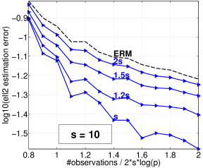
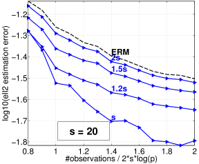
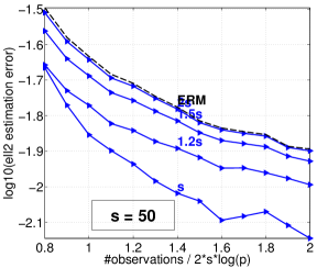
Figure 4: Sensitivity of ’IHT’ w.r.t. the choice of $s$. The plots display error curves of IHT run with the correct value of $s$ as appearing in Figure 3 as well with overspecification of $s$ by the factors $1.2,1.5,2$. The drop in performance is substantial: for $2s$, the improvement over ERM (here used as a reference) is only minor.

6.3 Density estimation

Let us recall the setup from the corresponding bullet in $\S$1. For simplicity, we here suppose that the $\{Z_{i}\}_{i=1}^{n}$ are i.i.d. random variables with density $\phi_{\beta^{*}}$, where for $\beta\in\Delta^{p}$, $\phi_{\beta}=\sum_{j=1}^{p}\phi_{j}\beta_{j}$ and $\mathcal{F}=\{\phi_{j}\}_{j=1}^{p}$ is a given collection of densities. Specifically, we consider univariate Gaussian densities $\phi_{j}=\phi_{\theta_{j}}$, where $\theta_{j}=(\mu_{j},\sigma_{j})$ contains mean and standard deviation, $j=1,\ldots,p$. As an example, one might consider $p_{0}$ locations and $K$ different standard deviations per location so that $p=p_{0}K$, i.e., $\theta_{(k-1)p_{0}+l}=(\mu_{l},\sigma_{k})$, $k=1,\ldots,K$, and $l=1,\ldots,p_{0}$. This construction provides more flexibility compared to usual kernel density estimation where the locations equal the data points, a single bandwidth is used, and the coefficients $\beta$ are all $1/n$. For large $\mathcal{F}$, sparsity in terms of the coefficients is common as a specific target density can typically be well approximated by using an appropriate subset of $\mathcal{F}$ of small cardinality.
As in Bunea et al. (2010), we work with the empirical risk

$$\vspace{-1ex}R_{n}(\beta)=\beta^{\top}Q\beta-2c^{\top}\beta,\quad c=\left(\textstyle\sum\nolimits_{i=1}^{n}\phi_{j}(Z_{i})/n\right)_{j=1}^{p},$$

and $Q=(\left\langle\phi_{j},\phi_{k}\right\rangle)_{j,k=1}^{p}$, where $\left\langle f,g\right\rangle=\int_{{\mathbb{R}}}fg$ for $f$,$g$ such that $\lVert f\rVert,\lVert g\rVert<\infty$ with $\lVert f\rVert=\left\langle f,f\right\rangle^{1/2}$.
In our simulations, we let $p_{0}=100$, $K=2$, $\sigma_{k}=k$, $k=1,2$. The locations $\{\mu_{l}\}_{l=1}^{p_{0}}$ are generated sequentially by selecting $\mu_{1}$ randomly from $[0,\delta]$, $\mu_{2}$ from $[\mu_{1}+\delta,\mu_{1}+2\delta]$ etc. where $\delta$ is chosen such that the ’correlations’ $\left\langle\phi_{j},\phi_{k}\right\rangle/\lVert\phi_{j}\rVert\lVert\phi_{k}\rVert\leq 0.5$ for all $(j,k)$ corresponding to different locations. An upper bound away from $1$ is needed to ensure identifiability of $S(\beta^{*})$ from finite samples. Data generation, the methods compared, and the way they are run is almost identical to the previous subsections. Slight changes are made for $S(\beta^{*})$ (still uniformly at random, but it is ruled that any location is selected twice), $b_{\min}^{*}$ ($\varrho$ set to $2$) and hyperparameter selection. For the latter, a separate validation data set (also of size $n$) is generated, and hyperparameters are selected as to minimize the empirical risk from the validation data.

Results. Figure 5 confirms once again that making use of simplex constraints yields markedly lower error than $\ell_{1}$-regularization followed by normalization (Bunea et al., 2010). ’L2-ERM’ and weighted $\ell_{1}$ perform best, improving over ’IHT’ (which is run with knowledge of $s$).

$\begin{array}[]{c}\includegraphics[width=178.50919pt]{plots/density/bw2/ell2/ell2_s_10}\\ {\tiny\begin{array}[]{l}\text{{Standard errors}(rounded):}\\ \begin{array}[]{|c|c|c|c|}\hline\cr\textbf{{L2-ERM}}&\textbf{{L2-D}}&\textbf{{ERM}}&\textbf{{Thres}}\\ .03&.03&.02&0.02\\ \hline\cr\textbf{{weightedL1}}&\textbf{{IHT}}&\textbf{{L1}}&\textbf{{oracle}}\\ .03&.03&.02&.02\\ \hline\cr\end{array}\end{array}}\end{array}$

$\begin{array}[]{c}\includegraphics[width=178.50919pt]{plots/density/bw2/ell2/ell2_s_20}\\ {\tiny\begin{array}[]{l}\text{{Standard errors}(rounded):}\\ \begin{array}[]{|c|c|c|c|}\hline\cr\textbf{{L2-ERM}}&\textbf{{L2-D}}&\textbf{{ERM}}&\textbf{{Thres}}\\ .02&.02&.02&0.02\\ \hline\cr\textbf{{weightedL1}}&\textbf{{IHT}}&\textbf{{L1}}&\textbf{{oracle}}\\ .02&.02&.01&.01\\ \hline\cr\end{array}\end{array}}\end{array}$

$\begin{array}[]{l}\includegraphics[width=105.69774pt]{plots/density/bw2_ell1/ell2/ell2_s_10}\\ \includegraphics[width=105.69774pt]{plots/density/bw2_ell1/ell2/ell2_s_20}\end{array}$

Figure 5: Average estimation errors $\lVert\widehat{\theta}-\beta^{*}\rVert_{2}$ for density estimation over 50 trials. Since the performance of ’L1’ falls short of the rest of the competitors, whose differences we would like to focus on, ’L1’ is compared to ’ERM’ and ’oracle’ in separate plots in the right column. Standard errors are smaller than $0.025$ for all methods.

6.4 Portfolio Optimization

We use a data set available from http://host.uniroma3.it/docenti/cesarone/datasetsw3_tardella.html containing the weekly returns of $p=2196$ stocks in the NASDAQ index collected during 03/2003 and 04/2008 (264 weeks altogether). For each stock, the expected returns is estimated as the mean return $\widehat{\mu}$ from the first four years (208 weeks). Likewise, the covariance of the returns is estimated as the sample covariance $\widehat{\Sigma}$ of the returns of the first four years. Given $\widehat{\mu}$ and $\widehat{\Sigma}$, portfolio selection (without short positions) is based on the optimization problem

$$\min_{\beta\in\Delta^{p}}\beta^{\top}\widehat{\Sigma}\beta-\tau\widehat{\mu}^{\top}\beta$$ (22)

where $\tau\in[0,\tau_{\max}]$ is a parameter controlling the trade-off between return and variance of the portfolio. Assuming that $\widehat{\mu}$ has a unique maximum entry, $\tau_{\max}$ is defined as the smallest number such that the solution of (22) has exactly one non-zero entry equal to one at the position of the maximum of $\widehat{\mu}$. As observed in Brodie et al. (2009), the solution of (22) tends to be sparse already because of the simplex constraint. Sparsity can be further enhanced with the help of the strategies discussed in this paper, treating (22) as the empirical risk. We here consider ’L2-ERM’, ’weighted L1’, ’Thres’ and ’IHT’ for a grid of values for the regularization parameter (’L2-ERM’ and ’weighted L1’) respectively sparsity level (’L2-ERM’ and ’Thres’). The solutions are evaluated by computing the Sharpe ratios (mean return divided by the standard deviation) of the selected portfolios on the return data of the last 56 weeks left out when computing $\widehat{\mu}$ and $\widehat{\Sigma}$.

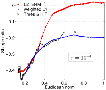
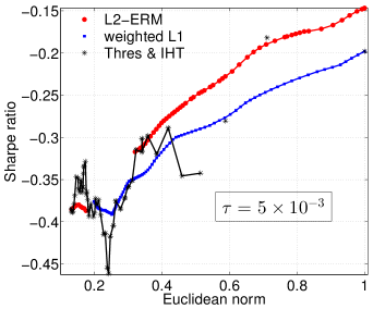
Figure 6: Sharpe ratios of the portfolios selected by ’L2-ERM’, ’weighted L1’, ’Thres’ and ’IHT’ on the hold-out portion of the NASDAQ data set in dependency of different choices for ther regularization parameter/sparsity level (to allow for joint display, we use the $\ell_{2}$-norm as measure of sparsity on the horizontal axis). Left panel: $\tau=10^{-4}$, Right panel: $\tau=5\cdot 10^{-3}$, cf. (22). The results of ’Thres’ and ’IHT’ are essentially indistinguishable and are hence not plotted separately for better readability. Note that points that are too far away from each other with respect to the horizontal axis are not connected by lines.

Results. Figure 6 displays the Sharpe ratios of the portfolios returned by these approaches in dependency of the $\ell_{2}$-norms of the solutions corresponding to different choices of the regularization parameter respectively sparsity level and two values of $\tau$ in (22). One observes that promoting sparsity is beneficial in general. The regularization-based methods ’L2-ERM’ and ’weighted L1’ differ from ’L2-ERM’ and ’Thres’ (whose results are essentially not distinguishable) in that the former two yield comparatively smooth curves. ’L2-ERM’ achieves the best Sharpe ratios for a wide range of $\ell_{2}$-norms for both values of $\tau$.

6.5 Quantum State Tomography

We now turn to the matrix case of Section 5. The setup of this subsection is based on model (15), where the measurements $\{X_{i}\}_{i=1}^{n}$ are chosen uniformly at random from the (orthogonal) Pauli basis of ${\mathbb{H}}^{m}$ (here, $m=2^{q}$ for some integer $q\geq 1$). For $q=1$, the Pauli basis of ${\mathbb{H}}^{2}$ is given by the following four matrices:

$$P_{1,1}=\begin{pmatrix}1&0\\ 0&1\end{pmatrix},\quad P_{1,2}=\begin{pmatrix}0&-\sqrt{-1}\\ \sqrt{-1}&0\end{pmatrix},\quad P_{1,3}=\begin{pmatrix}1&0\\ 0&-1\end{pmatrix},\quad P_{1,4}=\begin{pmatrix}0&1\\ 1&0\end{pmatrix}.$$

For $q>1$, the Pauli basis $\{P_{q,1},\ldots,P_{q,m^{2}}\}$is constructed as the $q$-fold tensor product of $\{P_{1,1},\ P_{1,2},\ P_{1,3},\ P_{1,4}\}$. The set of measurements is then given by $\{P_{q,i},i\in\mathcal{I}\}$, where $\mathcal{I}\subseteq\{1,\ldots,m^{2}\}$, $|\mathcal{I}|=n$, is chosen uniformly at random. Pauli measurements are commonly used in quantum state tomography in order to recover the density matrix of a quantum state (see Section 5 above). In Gross et al. (2010), it is shown that if $B^{*}$ is of low rank, it can be estimated accurately from few such random measurements by using nuclear norm regularization; the constraint $B^{*}\in\bm{\Delta}^{m}$ is not taken advantage of. Proposition 5 asserts that this constraint alone is well-suited for recovering matrices of low rank as long as the measurements satisfy a restricted strong convexity condition (Condition 2). It is shown in Liu (2011) that Pauli measurements satisfy the matrix RIP condition of Recht et al. (2010) as long as $n\gtrsim mr\log^{6}(m)$. Since the matrix RIP condition is stronger than Condition 2, Proposition 5 applies here. The requirement on $n$ is near-optimal: up to a polylogarithmic factor, it equals the ’degrees of freedom’ of the problem, which is given by $d=mr-r(r-1)/2\gtrsim mr$, which is the dimension of the space ${\mathbb{T}}(B^{*})\subset{\mathbb{H}}^{m}$ (cf. Definition E.1 in the appendix).

6.5.1 Noiseless measurements

In the first numerical study, we work with noiseless measurements. We fix $m=2^{7}$ and let $r\in\{1,2,5,10\}$ vary. The target is generated randomly as $B^{*}=AA^{\top}$, where $A$ is an $m\times r$ matrix, whose entries are drawn i.i.d. from $N(0,1)$. The number of random Pauli measurements $n$ are varied from $2d$ to $5d$ in steps of $0.5d$, where $d$ equals the ’degrees of freedom’ as defined above. For each possible combination of $n$ and $r$, $50$ trials are performed. The following three approaches for recovering $B^{*}$ are compared.

’Feasible set’: The counterpart to ERM in the noiseless case: finding a point in

$$\bm{D}(0)=\{B\in\bm{\Delta}^{m}:\;\mathcal{X}^{\star}(\mathcal{X}(B)-y)=0\}=\{B\in\bm{\Delta}^{m}:\mathcal{X}(B)=y\},$$ (23)

where the second identity follows from the orthogonality of the Pauli matrices.

’L2’: The counterpart to (18)/(19) in the noiseless case, which amounts to maximizing the Schatten $\ell_{2}$-norm (i.e., Frobenius norm) over (23). As initial iterate for Algorithm 1, the output from ’feasible set’ is used.

’IHT’: The matrix version of iterative hard thresholding under simplex constraints as proposed by Kyrillidis et al. (2013). Under the assumption that the rank of the target is known, one tries to solve directly the rank-constrained optimization problem $\min_{\bm{\Delta}_{0}^{m}(r)}R_{n}(B)$ using projected gradient descent. Projections onto $\bm{\Delta}_{0}^{m}(r)$ can be efficiently computed using partial eigenvalue decompositions. We use a constant step size as in Kyrillidis et al. (2013). The output of ’feasible set’ is used as initial iterate.

Results. Figure 7 shows a clear benefit of using $\ell_{2}$-norm maximization on top of solving the feasibility problem. For ’L2’, $2.5d$ measurements suffice to obtain highly accurate solutions, while ’feasible set’ requires $3.5d$ up to $5d$ measurements. The performance of IHT falls in between the two other approaches even though the knowledge of $r$ provides an extra advantage.

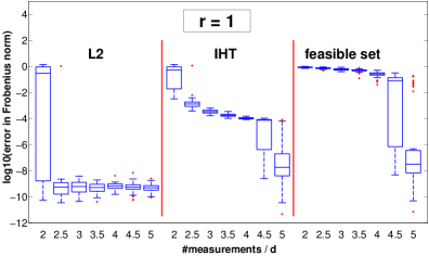
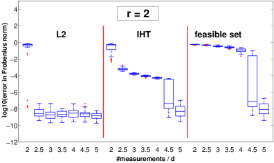
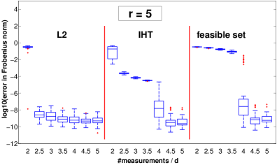
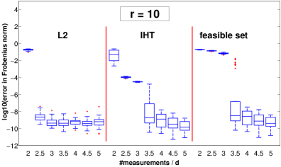
Figure 7: Boxplots of the errors $\lVert\widehat{\Theta}-B^{*}\rVert_{2}$ (50 trials) in recovering $B^{*}$ with respect to the Frobenius norm ($\log_{10}$ scale) in dependence of the number of Pauli measurements ($d=$ ’degrees of freedom’). Here, $\widehat{\Theta}$ is representative for any of the three estimators under consideration.

6.5.2 Noisy measurements

We maintain the setup of the previous paragraph, but the measurements are now subject to additive Gaussian noise with standard deviation $\sigma=0.1$. In order to adjust for the increased difficulty of the problem, the range for the number of measurements $n$ is multiplied by the factor $\log(m/r)$. Our comparison covers the following methods.
’ERM’: Empirical risk minimization, the counterpart to ’Feasible set’ above.
’Thres’: ’ERM’ followed by eigenvalue thresholding as outlined below Proposition 5.
’L2-ERM’: Regularized ERM with negative $\ell_{2}$-regularization (11). A grid search over 20 different values of the regularization parameter $\lambda$ is performed analogously to the vector case.
’weighted L1’: The approach in (17). The grid search for $\lambda$ follows the vector case.
’IHT’: As in the noiseless case.
’L1’: In analogy to the corresponding approach (7) in the vector case, the unit trace constraint is dropped, and a nuclear-norm regularized empirical risk is minimized over the positive semidefinite cone. The result is then divided by its trace. The regularization parameter is fixed to a single value $\lambda_{0}=2\sigma\sqrt{\log(m)/n}$ according to the literature (Negahban and Wainwright, 2011; Koltchinskii, 2011).

For ’Thres’, ’L2-ERM’ and other methods for which multiple values of a hyperparameter are considered, hyperparameter selection is done by minimizing a RIC-type criterion. Specifically, for some estimate $\widehat{\Theta}_{\lambda}$ of $B^{*}$, we use

$$\text{sel}(\lambda)=R_{n}(\widehat{\Theta}_{\lambda})+\frac{C\sigma^{2}\log(m^{2})\lVert\widehat{\Theta}_{\lambda}\rVert_{0}}{n}$$

The use of this criterion is justified in light of results in Klopp (2011) on trace regression with rank penalization. We have experimented with different choices of the constant $C$. Satisfactory results are achieved for $C=2^{6}$, which is the choice underlying the results displayed in Figure 8. Once $\lambda$ has been determined, the matrix of eigenvectors is fixed and the eigenvalues are re-fitted via least squares similar to (17).

Results. For space reasons, we only display the results for $r=2,10$ in Figures 8 and 9. ’IHT’ achieves best performance even though the error curve of ’L2’ is essentially identical for $r=2$. Figure 9 indicates that ’IHT’ is sensitive to the choice of $r$: over-specification by a factor of two can lead to a performance that is significantly worse than ’Thres’ and only slightly better than ’ERM’. Both ’L2’ and ’Thres’ are adaptive to the rank which is correctly recovered in almost all cases. In the matrix case, ’L2’ improves over ’Thres’ (as opposed to the vector case), possibly because for ’Thres’ the eigenvectors remain unchanged compared to ’ERM’, only the eigenvalues are modified. The performance of ’L1’ clearly falls short of all other competitors, which underpins the importance of the unit trace constraint.

$\begin{array}[]{c}\includegraphics[width=164.4171pt]{plots/tomography_noisy/errs_2/errs_2_r2.eps}\\ {\scriptsize\begin{array}[]{l}\text{{Standard errors}(rounded):}\\ \begin{array}[]{|c|c|c|}\hline\cr\textbf{{L2-ERM}}&\textbf{{ERM}}&\textbf{{Thres}}\\ 3\cdot 10^{-3}&3\cdot 10^{-3}&3\cdot 10^{-3}\\ \hline\cr\textbf{{weightedL1}}&\textbf{{IHT}}&\textbf{{L1}}\\ 1.4\cdot 10^{-2}&3\cdot 10^{-3}&1.7\cdot 10^{-2}\\ \hline\cr\end{array}\end{array}}\end{array}$

$\begin{array}[]{c}\includegraphics[width=164.4171pt]{plots/tomography_noisy/errs_2/errs_2_r10.eps}\\ {\scriptsize\begin{array}[]{l}\text{{Standard errors}(rounded):}\\ \begin{array}[]{|c|c|c|}\hline\cr\textbf{{L2-ERM}}&\textbf{{ERM}}&\textbf{{Thres}}\\ 2\cdot 10^{-3}&1.2\cdot 10^{-2}&1.7\cdot 10^{-2}\\ \hline\cr\textbf{{weightedL1}}&\textbf{{IHT}}&\textbf{{L1}}\\ 1.2\cdot 10^{-2}&1.1\cdot 10^{-2}&8\cdot 10^{-3}\\ \hline\cr\end{array}\end{array}}\end{array}$

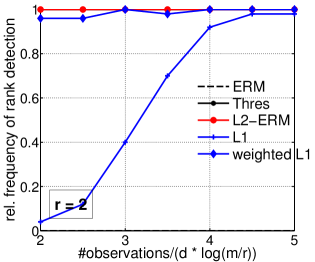
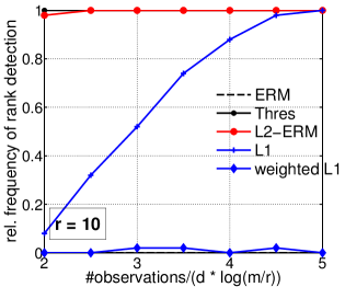
Figure 8: Bottom: Average estimation errors $\lVert\widehat{\Theta}-B^{*}\rVert_{2}$ over 50 trials ($\log_{10}$-scale) in dependence of the number of measurements ($d=$ ’degrees of freedom’). Top: Relative frequency of rank detection, i.e., of the event $\{\lVert\widehat{\Theta}\rVert_{0}=\lVert B^{*}\rVert_{0}\}$; for ’IHT’ this relative frequency is always one, which is not shown in the plots. Here, $\widehat{\Theta}$ is representative for any of the estimators under consideration.

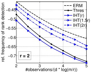
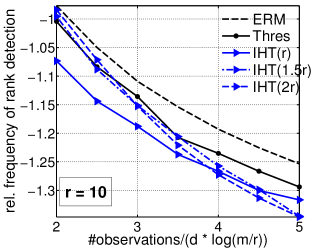
Figure 9: Sensitivity of ’IHT’ w.r.t. the choice of $r$. The dashed-dotted and dashed lines show the average estimation errors when ’IHT’ is run with $1.5r$ and $2r$, respectively. The results of ’Thres’ and ’ERM’ serve as reference.

7 Conclusion

Simplex constraints are beneficial in high-dimensional estimation, typically achieving noticeably lower estimation error than using $\ell_{1}$-norm regularization in place of the constraint. In order to enhance sparsity of the solution, simple two-stage methods - thresholding and weighted $\ell_{1}$-regularization - can be rather effective. A more principled way to incorporate sparsity is the use of a suitable regularizer. We have pointed out that under simplex constraints, sparsity cannot be promoted by convex regularizers. We have therefore considered non-convex alternatives among which regularization by means of the negative $\ell_{2}$-norm turns out to be a natural approach lending itself to a straightforward computational strategy. As an attractive feature, there is a direct and practical generalization to the matrix counterpart as opposed to the two-stage methods.

Appendix A Proof of Proposition 1

By definition of $\widehat{\beta}$, we have

$$R_{n}(\widehat{\beta})\leq R_{n}(\beta^{*})$$

$$\Rightarrow\quad \{R_{n}(\widehat{\beta})-R(\widehat{\beta})\}+R(\widehat{\beta})\leq\{R_{n}(\beta^{*})-R(\beta^{*})\}+R(\beta^{*})$$

$$\Rightarrow\quad R(\widehat{\beta})\leq R(\beta^{*})+\sup_{\beta\in\mathbb{B}_{1}^{p}(\lVert\widehat{\beta}-\beta^{*}\rVert_{1};\beta^{*})}|\underbrace{\{R_{n}(\beta)-\{R_{n}(\beta^{*})\}-\{R(\beta)-R(\beta^{*})\}}_{\overline{\psi}_{n}(\beta)}|$$

$$\qquad=R(\beta^{*})+\overline{\Psi}_{n}(\lVert\widehat{\beta}-\beta^{*}\rVert_{1})$$

$$\qquad\leq R(\beta^{*})+\overline{\Psi}_{n}(2).$$

The last inequality follows from $\widehat{\beta}\in\Delta^{p}$, $\beta^{*}\in\Delta^{p}$ and the triangle inequality.
We now turn to $\widetilde{\beta}_{\lambda}$. Consider the curve (segment) $\gamma(t)=\beta^{*}+t(\widetilde{\beta}_{\lambda}-\beta^{*})$ for $t\in[0,1]$ and the function $g(t)=R_{n}(\beta^{*}+t(\widetilde{\beta}_{\lambda}-\beta^{*}))$. Then $g=R_{n}\circ\gamma$ is convex, as it is the composition of an affine and a convex function. Consequently, the derivative

$$g^{\prime}(t)=\nabla R_{n}(\beta^{*}+t(\widetilde{\beta}_{\lambda}-\beta^{*}))^{\top}(\widetilde{\beta}_{\lambda}-\beta^{*})$$

is non-decreasing. As a result, we have

$$R_{n}(\widetilde{\beta}_{\lambda})-R_{n}(\beta^{*}) =\int_{0}^{1}\nabla R_{n}(\beta^{*}+t(\widetilde{\beta}_{\lambda}-\beta^{*}))^{\top}(\widetilde{\beta}_{\lambda}-\beta^{*})\;dt$$

$$\leq\nabla R_{n}(\widetilde{\beta}_{\lambda})^{\top}(\widetilde{\beta}_{\lambda}-\beta^{*})$$

$$\leq\lVert\nabla R_{n}(\widetilde{\beta}_{\lambda})\rVert_{\infty}\lVert\widetilde{\beta}_{\lambda}-\beta^{*}\rVert_{1}$$

$$\leq\lambda\lVert\widetilde{\beta}_{\lambda}-\beta^{*}\rVert_{1},$$

where the first inequality follows from the definition and monotonicity property of $g^{\prime}$, the second inequality is Hölder’s inequality and the last inequality follows from the definition of $\widetilde{\beta}_{\lambda}$. Given the above upper bound on $R_{n}(\widetilde{\beta}_{\lambda})-R_{n}(\beta^{*})$, the proof can be completed by following the scheme used for $\widehat{\beta}$.

Appendix B Proof of Proposition 2

We have

$$R_{n}(\widehat{\beta})-R_{n}(\beta^{*})-\nabla R_{n}(\beta^{*})^{\top}(\widehat{\beta}-\beta^{*})\geq\kappa\lVert\widehat{\beta}-\beta^{*}\rVert_{2}^{2},$$

by the $\Delta$-RSC. On the other hand, by the definition of $\widehat{\beta}$

$$R_{n}(\widehat{\beta})-R_{n}(\beta^{*})-\nabla R_{n}(\beta^{*})^{\top}(\widehat{\beta}-\beta^{*}) \leq-\nabla R_{n}(\beta^{*})^{\top}(\widehat{\beta}-\beta^{*})$$

$$\leq\lVert\nabla R_{n}(\beta^{*})\rVert_{\infty}\lVert\widehat{\beta}-\beta^{*}\rVert_{1}.$$

Combining these two bounds, we obtain that

$$\kappa\lVert\widehat{\beta}-\beta^{*}\rVert_{2}^{2}\leq\lVert\nabla R_{n}(\beta^{*})\rVert_{\infty}\lVert\widehat{\beta}-\beta^{*}\rVert_{1}.$$

This implies that

$$\lVert\widehat{\beta}-\beta^{*}\rVert_{2}^{2}\leq\frac{\lVert\nabla R_{n}(\beta^{*})\rVert_{\infty}^{2}}{\kappa^{2}}\left(\frac{\lVert\widehat{\beta}-\beta^{*}\rVert_{1}}{\lVert\widehat{\beta}-\beta^{*}\rVert_{2}}\right)^{2}\leq\frac{4s\lambda_{*}^{2}}{\kappa^{2}},$$

$$\lVert\widehat{\beta}-\beta^{*}\rVert_{1}\leq\frac{\lVert\nabla R_{n}(\beta^{*})\rVert_{\infty}}{\kappa}\left(\frac{\lVert\widehat{\beta}-\beta^{*}\rVert_{1}}{\lVert\widehat{\beta}-\beta^{*}\rVert_{2}}\right)^{2}\leq\frac{4s\lambda_{*}}{\kappa},$$

where $\lambda_{*}=\lVert\nabla R_{n}(\beta^{*})\rVert_{\infty}$. The rightmost inequalities follow from the fact that $\widehat{\beta}-\beta^{*}\in\mathcal{C}^{\Delta}(s)$ and hence $\lVert\widehat{\beta}_{S(\beta^{*})^{c}}\rVert_{1}\leq\lVert\widehat{\beta}_{S(\beta^{*})}-\beta_{S(\beta^{*})}^{*}\rVert_{1}$ so that

$$\lVert\widehat{\beta}-\beta^{*}\rVert_{1} =\lVert\widehat{\beta}_{S(\beta^{*})}-\beta_{S(\beta^{*})}^{*}\rVert_{1}+\lVert\widehat{\beta}_{S(\beta^{*})^{c}}\rVert_{1}$$

$$\leq 2\lVert\widehat{\beta}_{S(\beta^{*})}-\beta_{S(\beta^{*})}^{*}\rVert_{1}\leq 2\sqrt{s}\lVert\widehat{\beta}_{S(\beta^{*})}-\beta_{S(\beta^{*})}^{*}\rVert_{2}.$$

We now turn to $\widetilde{\beta}_{\lambda}$. Starting from

$$R_{n}(\widetilde{\beta}_{\lambda})-R_{n}(\beta^{*})-\nabla R_{n}(\beta^{*})^{\top}(\widetilde{\beta}_{\lambda}-\beta^{*})\geq\kappa\lVert\widetilde{\beta}_{\lambda}-\beta^{*}\rVert_{2}^{2},$$

and using the upper bound on $R_{n}(\widetilde{\beta}_{\lambda})-R_{n}(\beta^{*})$ as derived in the proof of Proposition 1, we obtain

$$\kappa\lVert\widetilde{\beta}_{\lambda}-\beta^{*}\rVert_{2}^{2} \leq\lVert\nabla R_{n}(\widetilde{\beta}_{\lambda})\rVert_{\infty}\lVert\widetilde{\beta}_{\lambda}-\beta^{*}\rVert_{1}+\lVert\nabla R_{n}(\beta^{*})\rVert_{\infty}\lVert\widetilde{\beta}_{\lambda}-\beta^{*}\rVert_{1}$$

$$\leq(\lambda+\lambda_{*})\lVert\widetilde{\beta}_{\lambda}-\beta^{*}\rVert_{1},$$

Arguing similarly as for $\widehat{\beta}$, it follows that

$$\lVert\widetilde{\beta}_{\lambda}-\beta^{*}\rVert_{2}^{2}\leq\frac{4s(\lambda+\lambda_{*})^{2}}{\kappa^{2}},\qquad\lVert\widetilde{\beta}_{\lambda}-\beta^{*}\rVert_{1}\leq\frac{4s(\lambda+\lambda_{*})}{\kappa}.$$

Appendix C Proof of Proposition 4

We prove the statement for problem (11)

$$\min_{\beta\in\Delta^{p}}R_{n}(\beta)-\lambda\left\lVert\beta\right\rVert^{2}_{2}.$$ (24)

The proof for problem (12) follows similarly. The subproblem solved in each iteration in the case of (24) is given by

$$\min_{\beta\in\Delta^{p}}R_{n}(\beta)-2\lambda\left\langle\beta^{k},\beta-\beta^{k}\right\rangle$$ (25)

First note that the constraint sets of both (24) and (25) are compact and the objectives are continuous, hence these problems have at least one minimizer by Weierstrass theorem and the minima are finite.

The current iterate $\beta^{k}$ is always feasible for (25). Hence the optimal value of (25) is either $R_{n}(\beta^{k})$ (in which case the algorithm terminates) or strictly smaller than $R_{n}(\beta^{k})$,

$$R_{n}(\beta^{k+1})-2\lambda\left\langle\beta^{k},\beta^{k+1}-\beta^{k}\right\rangle<R_{n}(\beta^{k}).$$ (26)

On the other hand, by convexity of $\lambda\left\lVert\beta\right\rVert^{2}_{2}(\lambda\geq 0)$, we have

$$f(\beta^{k+1})=R_{n}(\beta^{k+1})-\lambda\left\lVert\beta^{k+1}\right\rVert_{2}^{2} \leq R_{n}(\beta^{k+1})-\lambda\left\lVert\beta^{k}\right\rVert_{2}^{2}-2\lambda\left\langle\beta^{k},\beta^{k+1}-\beta^{k}\right\rangle$$

$$\stackrel{{\scriptstyle\eqref{eq:descent}}}{{<}}R_{n}(\beta^{k})-\lambda\left\lVert\beta^{k}\right\rVert_{2}^{2}$$

$$=f(\beta^{k})$$

This establishes the strict monotonicity of the iterates in terms of the objective $f$ of the original problem (24) until convergence. It is clear that all the elements of the sequence $\{\beta^{k}\}$ are feasible for (24) and satisfy $f^{*}\leq f(\beta^{k}),\ k\geq 0$, where $f^{*}$ is the global minimum of (24). Since $\{f(\beta^{k})\}$ is a strictly decreasing sequence bounded below by a finite $f^{*}$, the sequence converges to a limit

$$\bar{f}=\lim_{k\rightarrow\infty}f(\beta^{k}).$$

Since all the elements of the sequence $\{\beta^{k}\}$ are contained in $\Delta^{p}$, a compact set, there exists a subsequence $\{\beta^{k_{i}}\}$ converging to an element $\bar{\beta}\in\Delta^{p}$. The sequence $\{f(\beta^{k_{i}})\}$ is a subsequence of $\{f(\beta^{k})\}$ that is shown to converge to the limit $\bar{f}$; hence the subsequence $\{f(\beta^{k_{i}})\}$ also converges to the same limit

$$\lim_{k\rightarrow\infty}f(\beta^{k_{i}})=\bar{f}.$$

Let us define $\phi_{\bar{\beta}}(\beta)=R_{n}(\beta)-2\lambda\left\langle\bar{\beta},\beta-\bar{\beta}\right\rangle$. We now argue that $\bar{\beta}\in\operatorname*{argmin}_{\beta\in\Delta^{p}}\phi_{\bar{\beta}}(\beta)$. To see this note that $\bar{\beta}$ is feasible for this problem and hence $\min_{\beta\in\Delta^{p}}\phi_{\bar{\beta}}(\beta)\leq f(\bar{\beta})=\bar{f}$. Assume for the sake of contradiction that a minimizer $\check{\beta}$ of this problem has a strictly smaller objective,

$$\phi_{\bar{\beta}}(\check{\beta})=R_{n}(\check{\beta})-2\lambda\left\langle\bar{\beta},\check{\beta}-\bar{\beta}\right\rangle<\bar{f}.$$

Similar to the argument above regarding strict descent, we can show that

$$f(\check{\beta})<\bar{f},$$

which contradicts the fact that the sequence $\{f(\beta^{k})\}$ has converged to the limit $\bar{f}$. Thus, we must have,

$$\bar{\beta}\in\operatorname*{argmin}_{\beta\in\Delta^{p}}R_{n}(\beta)-2\lambda\left\langle\bar{\beta},\beta-\bar{\beta}\right\rangle.$$

The first order optimality condition for $\bar{\beta}$ then implies

$$-\nabla R_{n}(\bar{\beta})+2\lambda\bar{\beta}\in N_{\Delta^{p}}(\bar{\beta}),$$

where $N_{\Delta^{p}}(\bar{\beta})$ is the normal cone of $\Delta^{p}$ at $\bar{\beta}$ (see e.g. Rockafellar and Wets (2004) for a definition). Note that this is exactly the first-order optimality condition for the original problem (24). Finally note that the argument is true for any subsequence $\{\beta^{k_{i}}\}$ and hence each of such subsequences and consequently the original sequence $\{\beta^{k}\}$ converge to the same limit $\bar{\beta}$, which has been shown to satisfy the required optimality condition.

Appendix D Proof of Proposition 3

The optimization problem under consideration is equivalent to the following one:

$$\min_{\beta\in\Delta^{n}}\left(\frac{1}{n}-\lambda\right)\lVert\beta\rVert_{2}^{2}-\frac{2}{n}\mathbf{Z}^{\top}\beta.$$ (27)

For $\lambda\geq 1/n$, the objective becomes concave. If $\lambda>1/n$, the objective is strictly concave and the unique minimum is attained at one of the vertices $\{e_{i}\}_{i=1}^{n}$ of $\Delta^{n}$. It must be any unit vector $e_{i}$ for which $z_{i}=\max_{1\leq k\leq n}z_{k}$. Since we have assumed that $z_{(1)}>\ldots>z_{(n)}$, such vector is unique. If $\lambda=1/n$, we have

$$\widehat{\beta}_{\lambda}^{\ell_{2}}\in\operatorname*{conv}\left\{e_{i}:\;z_{i}=\max_{1\leq k\leq n}z_{k}\right\}.$$

By the same argument as above, that convex hull equals the unique unit vector $e_{i}$ for which $z_{i}=\max_{1\leq k\leq n}z_{k}$.
For $0\leq\lambda<1/n$, the problem becomes strictly convex. Setting $\gamma=1-n\lambda$, problem (27) is equivalent to

$$\min_{\beta\in\Delta^{n}}\gamma\lVert\beta\rVert_{2}^{2}-2\mathbf{Z}^{\top}\beta.$$

Re-arranging terms, this can be seen to be equivalent to

$$\min_{\beta\in\Delta^{n}}\left\lVert\beta-\frac{\mathbf{Z}}{\gamma}\right\rVert_{2}^{2},$$

i.e. $\widehat{\beta}_{\lambda}^{\ell_{2}}=\Pi_{\Delta^{n}}(\mathbf{Z}/\gamma)$, with $\Pi_{\Delta^{n}}$ denoting the Euclidean projection onto $\Delta^{n}$.
Suppose that the realizations $\mathbf{z}=(z_{i})_{i=1}^{n}$ are arranged such that

$$z_{1}=\beta_{1}^{*}+\varepsilon_{1}>z_{2}=\beta_{2}^{*}+\varepsilon_{2}>\ldots>z_{s}=\beta_{s}^{*}+\varepsilon_{s}>z_{s+1}=\varepsilon_{s+1}>\ldots>z_{p}=\varepsilon_{p}.$$

Under the event $\{b_{\min}^{*}=\min_{i\in S(\beta^{*})}|\beta_{i}^{*}|\geq 2\max_{1\leq i\leq n}|\varepsilon_{i}|\}$, this can be assumed without loss of generality. The projection of $\mathbf{z}/\gamma$ onto $\Delta^{n}$ can then can be expressed as (cf. Kyrillidis et al. (2013))

$$\left(\Pi_{\Delta^{n}}(\mathbf{z}/\gamma)\right)_{i}=\max\{z_{i}/\gamma-\tau,0\},\quad\text{where}\;\tau=\frac{1}{q}\left(\sum_{i=1}^{q}(z_{i}/\gamma)-1\right),$$

and

$$q=\max\left\{k:\;(z_{k}/\gamma)>\frac{1}{k}\left(\sum_{i=1}^{k}(z_{i}/\gamma)-1\right)\right\}.$$

In order to establish that $S(\widehat{\beta}_{\lambda}^{\ell_{2}})=S(\beta^{*})$, it remains to be shown that under the given conditions on $b_{\min}^{*}$ and $\lambda$ respectively $\gamma$, it holds that

$$(a)\quad \frac{\beta_{s}^{*}+\varepsilon_{s}}{\gamma}>\frac{1}{\gamma}\frac{\beta_{1}^{*}+\ldots+\beta_{s}^{*}-\gamma}{s}+\frac{1}{\gamma}\frac{\varepsilon_{1}+\ldots+\varepsilon_{s}}{s}=\frac{1}{s}\,\frac{1-\gamma}{\gamma}+\frac{1}{\gamma}\frac{\varepsilon_{1}+\ldots+\varepsilon_{s}}{s}$$

$$\Longleftrightarrow \;\beta_{s}^{*}>\frac{1}{s}(\{1-\gamma\}-\left\{\varepsilon_{1}+\ldots+\varepsilon_{s}-s\varepsilon_{s}\right\}).$$

and

$$(b)\quad\frac{\varepsilon_{s+1}}{\gamma}<\frac{1}{\gamma}\frac{1-\gamma}{s+1}+\frac{1}{\gamma}\frac{\varepsilon_{1}+\ldots+\varepsilon_{s}+\varepsilon_{s+1}}{s+1}.$$

Re-arranging (b), we find that

$$n\lambda=(1-\gamma)>s\varepsilon_{s+1}-(\varepsilon_{1}+\ldots+\varepsilon_{s}),$$

which is implied by

$$n\lambda>2s\max_{1\leq i\leq n}|\varepsilon_{i}|.$$

Likewise, the inequality in (a) holds as long as

$$\beta_{s}^{*}>\frac{n\lambda}{s}+2\max_{i}|\varepsilon_{i}|.$$

This concludes the proof.

Appendix E Proof of Proposition 5

Before providing a proof of Proposition 5, we first provide a precise definition of the linear spaces ${\mathbb{T}}(B)$, $B\in\bm{B}_{0}^{m}(r)\subset{\mathbb{H}}^{m}$.

Definition E.1.

Let $B\in\bm{B}_{0}^{m}(r)$ have eigenvalue decomposition $B=U\Lambda U^{H}$, where

$$U=\left[\begin{array}[]{cc}U_{\parallel}&U_{\perp}\\ \mbox{{\footnotesize$m\times r$}}&\mbox{{\footnotesize$m\times(m-r)$}}\end{array}\right]\begin{bmatrix}\Lambda_{r}&0_{r\times(m-r)}\\ 0_{(m-r)\times r}&0_{(m-r)\times(m-r)}\end{bmatrix}$$

for $\Lambda_{r}$ real and diagonal. We then define

$${\mathbb{T}}(B)=\{M\in\mathbb{H}^{m}:\;M=U_{\parallel}\Gamma+\Gamma^{H}U_{\parallel}^{H},\quad\Gamma\in{\mathbb{C}}^{r\times m}\}.$$

It is immediate from the definition of ${\mathbb{T}}(B)$ that its orthogonal complement is given by

$$\mathbb{T}(B)^{\perp}=\{M\in\mathbb{H}^{m}:\;M=U_{\perp}AU_{\perp}^{H},\quad A\in\mathbb{H}^{m-r}\}.$$

Proof.

We first show that $\widehat{\Phi}=\widehat{B}-B^{*}\in\mathcal{K}^{\bm{\Delta}}(r)$, where we recall that

$$\mathcal{K}^{\bm{\Delta}}(r)=\{\Phi\in\mathbb{H}^{m}:\,\exists B\in\bm{B}_{0}^{m}(r)\,\text{s.t.}$$

$$\operatorname*{tr}(\Pi_{\mathbb{T}(B)^{\perp}}(\Phi))=-\operatorname*{tr}(\Pi_{\mathbb{T}(B)}\Phi)\;\text{and}\;\Pi_{\mathbb{T}(B)^{\perp}}(\Phi)\succeq 0\}.$$

Define the shortcuts $\widehat{\Phi}_{{\mathbb{T}}}=\Pi_{\mathbb{T}(B^{*})}\widehat{\Phi}$ and $\widehat{\Phi}_{{\mathbb{T}}^{\perp}}=\Pi_{\mathbb{T}(B^{*})^{\perp}}\widehat{\Phi}$. Since $\widehat{B}$ is feasible, it must hold that $\operatorname*{tr}(\widehat{\Phi})=0$ and thus $\operatorname*{tr}(\widehat{\Phi}_{{\mathbb{T}}^{\perp}})=-\operatorname*{tr}(\widehat{\Phi}_{{\mathbb{T}}})$. Since $\widehat{B}$ must also be positive definite, it must hold that $\operatorname*{tr}(\widehat{B}{W})\geq 0$ for all $W\in{\mathbb{T}}(B^{*})^{\perp}$, $W\succeq 0$. We have

$$\operatorname*{tr}(\widehat{B}{W})=\operatorname*{tr}((B^{*}+\widehat{\Phi})W)=\operatorname*{tr}(\widehat{\Phi}_{{\mathbb{T}}^{\perp}}W)\;\;\forall W\in{\mathbb{T}}(B^{*})^{\perp},$$

since $B^{*}\in{\mathbb{T}}(B^{*})$. We conclude that $\operatorname*{tr}(\widehat{\Phi}_{{\mathbb{T}}^{\perp}}W)\geq 0$ for all $W\in{\mathbb{T}}(B^{*})^{\perp}$, $W\succeq 0$, and thus $\widehat{\Phi}_{{\mathbb{T}}^{\perp}}\succeq 0$. Altogether, we have shown that $\widehat{\Phi}\in\mathcal{K}^{\bm{\Delta}}(r)$.
Since $\widehat{B}$ is a minimizer, we have

$$\frac{1}{n}\lVert\mathbf{Y}-\mathcal{X}(\widehat{B})\rVert_{2}^{2}\leq\frac{1}{n}\lVert\mathbf{Y}-\mathcal{X}(B^{*})\rVert_{2}^{2}\\$$

After re-arranging terms, we obtain

$$\frac{1}{n}\lVert\mathcal{X}(B^{*}-\widehat{B})\rVert_{2}^{2} \leq\frac{2}{n}\left\langle\varepsilon,\mathcal{X}(\widehat{B}-B^{*})\right\rangle$$

$$=\frac{2}{n}\left\langle\mathcal{X}^{\star}(\varepsilon),\widehat{B}-B^{*}\right\rangle$$

$$\leq 2\lVert\mathcal{X}^{\star}(\varepsilon)/n\rVert_{\infty}\lVert\widehat{B}-B^{*}\rVert_{1}$$

$$=\lambda_{*}\lVert\widehat{B}-B^{*}\rVert_{1}.$$

where $\mathcal{X}^{\star}$ is the adjoint of $\mathcal{X}$. By $\bm{\Delta}$-RSC, we now have

$$\frac{1}{n}\lVert\mathcal{X}(B^{*}-\widehat{B})\rVert_{2}^{2}\geq\kappa\lVert B^{*}-\widehat{B}\rVert_{2}^{2}.$$

Combining this with the preceding upper bound, we hence obtain

$$\lVert\widehat{B}-B^{*}\rVert_{2}^{2}\leq\frac{\lambda_{*}^{2}}{\kappa^{2}}\left(\frac{\lVert\widehat{B}-B^{*}\rVert_{1}}{\lVert\widehat{B}-B^{*}\rVert_{2}}\right)^{2}\leq\frac{8r\lambda_{*}^{2}}{\kappa^{2}},$$

$$\lVert\widehat{B}-B^{*}\rVert_{1}\leq\frac{\lambda_{*}}{\kappa}\left(\frac{\lVert\widehat{B}-B^{*}\rVert_{1}}{\lVert\widehat{B}-B^{*}\rVert_{2}}\right)^{2}\leq\frac{8r\lambda_{*}}{\kappa},$$

The rightmost inequalities follow from the fact that $\widehat{B}-B^{*}=\widehat{\Phi}\in\mathcal{K}^{\bm{\Delta}}(r)$ and hence $\lVert\widehat{\Phi}_{{\mathbb{T}}^{\perp}}\rVert_{1}\leq\lVert\widehat{\Phi}_{{\mathbb{T}}}\rVert_{1}$ so that

$$\lVert\widehat{B}-B^{*}\rVert_{1}=\lVert\widehat{\Phi}\rVert_{1} =\lVert\widehat{\Phi}_{{\mathbb{T}}}\rVert_{1}+\lVert\widehat{\Phi}_{{\mathbb{T}}^{\perp}}\rVert_{1}$$

$$\leq 2\lVert\widehat{\Phi}_{{\mathbb{T}}}\rVert_{1}$$

$$\leq 2\sqrt{2r}\lVert\widehat{\Phi}_{{\mathbb{T}}}\rVert_{2}\leq 2\sqrt{2r}\lVert\widehat{B}-B^{*}\rVert_{2},$$

where for the third inequality, we have used that $\lVert M\rVert_{0}\leq 2r$ for all $M\in{\mathbb{T}}(B^{*})$.
The bound for $\widetilde{B}_{\lambda}$ can be established by combining the proof scheme used for $\widetilde{\beta}_{\lambda}$ with the scheme used for $\widehat{B}$ and is thus omitted. ∎

Appendix F Proof of Proposition 6

We start by expanding the objective function of the optimization problem under consideration. Define $\mathbb{S}^{m}:{\mathbb{H}}^{m}\cap{\mathbb{R}}^{m\times m}$ which is a subspace of ${\mathbb{H}}^{m}$ which is isometrically isomorphic (w.r.t. to the standard inner product) to ${\mathbb{R}}^{\delta_{m}}$, $\delta_{m}=m(m+1)/2$ under the isometry $\mathcal{X}$ (20). Therefore,

$$\frac{1}{n}\lVert\mathbf{Y}-\mathcal{X}(B)\rVert_{2}^{2} =\frac{1}{n}\lVert\mathcal{X}^{\star}(\mathbf{Y})-B\rVert_{2}^{2}$$

$$=\frac{1}{n}\lVert B^{*}+E-B\rVert_{2}^{2},\quad E\mathrel{\mathop{:}}=\mathcal{X}^{\star}(\varepsilon),$$

$$=\frac{1}{n}\lVert\Upsilon-B\rVert_{2}^{2},\quad\Upsilon\mathrel{\mathop{:}}=B^{*}+E.$$ (28)

It follows directly from the definition of $\mathcal{X}^{\star}$ that the symmetric random matrix $E=(\varepsilon_{jk})_{1\leq j,k\leq m}$ is distributed according to the Gaussian orthogonal ensemble (GOE, see e.g. Tao (2012)), i.e., $E\sim\text{GOE}(m)$, where

$$\vspace*{-1ex}\text{GOE}(m)=\{X=(x_{jk})_{1\leq j,k\leq m},\; \{x_{jj}\}_{j=1}^{m}\overset{\text{i.i.d.}}{\sim}N(0,1/m),$$

$$\{x_{jk}=x_{kj}\}_{1\leq j<k\leq m}\overset{\text{i.i.d.}}{\sim}N(0,1/2m)\}.$$

In virtue of (28), we have

$$\min_{B\in\bm{\Delta}^{m}}\frac{1}{n}\lVert\mathbf{Y}-\mathcal{X}(B)\rVert_{2}^{2} =\min_{B\in\bm{\Delta}^{m}}\left\{(1/n-\lambda)\lVert B\rVert_{2}^{2}-\frac{2}{n}\left\langle\Upsilon,B\right\rangle\right\}+\frac{1}{n}\lVert\Upsilon\rVert_{2}^{2}.$$

At this point, the proof parallels the proof of Proposition 3. We see that for $\lambda\geq 1/n$, $\widehat{B}_{\lambda}^{\ell_{2}}=u_{1}u_{1}^{\top}$, where $u_{1}$ is the eigenvector of $\Upsilon$ corresponding to its largest eigenvalue. This follows from the duality of the Schatten $\ell_{1}$/$\ell_{\infty}$ norms and the fact that for all feasible $B$, it holds that $\lVert B\rVert_{2}^{2}\leq\lVert B\rVert_{1}^{2}=1$ with equality if and only if $B$ has rank one. Conversely, if $0\leq\lambda<1/n$, we define $\gamma\mathrel{\mathop{:}}=1-n\lambda>0$ and deduce that the optimization problem in the previous display is equivalent to $\min_{B\in\bm{\Delta}^{m}}\lVert\Upsilon/\gamma-B\rVert_{2}^{2}$ with minimizer $\widehat{B}_{\lambda}^{\ell_{2}}=U\text{diag}(\{\widehat{\phi}_{j}\}_{j=1}^{m})U^{\top}$, where $\widehat{\phi}=\Pi_{\Delta^{m}}(\upsilon/\gamma)$ with $\upsilon=(\upsilon_{j})_{j=1}^{m}$ denoting the eigenvalues of $\Upsilon$ (in decreasing order) corresponding to the eigenvectors in $U$. We now prove the last claim of the proposition, combining the proof of Proposition 3 for the vector case with concentration results by Peng (2012) for the spectrum of the random matrix $\Upsilon=B^{*}+E$, which are here rephrased as follows. Define

$$\widetilde{\phi}_{j}^{*}=\begin{cases}\phi_{j}^{*}+\frac{\sigma^{2}}{\phi_{j}^{*}}\quad&\text{if}\;\sigma<\phi_{j}^{*}\leq 1\\ 2\sigma\quad&\text{if}\;0\leq\phi_{j}^{*}\leq\sigma,\quad j=1,\ldots,m,\end{cases}$$

where we recall that the $\{\phi_{j}^{*}\}_{j=1}^{m}$ denote the ordered eigenvalues of $B^{*}$ and $\sigma^{2}$ is the variance of the noise (up to a scaling factor of $1/m$). We then have

$$\operatorname*{\mathbf{P}}(\upsilon_{j}\geq\widetilde{\phi}_{j}^{*}+t) \leq C_{1}\exp(-c_{1}mt^{2}/\sigma^{2}),\quad j=1,\ldots,m.$$

Furthermore, let $r_{0}$ denote the number of eigenvalues of $B^{*}$ that are larger than $\sigma$. Then, there is a constant $c_{0}>0$ so that if $r\leq c_{0}m$, it holds that

$$\operatorname*{\mathbf{P}}(\upsilon_{j}\leq\widetilde{\phi}_{j}^{*}-t-2\sigma) \leq\exp(-c_{2}m/\sigma^{2})+C_{2}^{\prime}\exp(-c_{2}^{\prime}mt^{2}/\sigma^{2}),\quad j=1,\ldots,r_{0},$$

where $c_{1},c_{2},C_{1},C_{2},C_{2}^{\prime}$ are positive constants.
It needs to be shown that for a suitable choice of $\lambda$ and for $\phi_{r}^{*}$ large enough, it holds that $\lVert\widehat{B}_{\lambda}^{\ell_{2}}\rVert_{0}=\lVert B^{*}\rVert_{0}=r$ with high probability as specified in the proposition. This is the case if and only if $\widehat{\phi}=\Pi_{\Delta^{m}}(\upsilon/\gamma)$ has precisely $r$ non-zero entries.

a) $\lVert\widehat{\phi}\rVert_{0}\geq r$:
It follows from the proof in the vector case that a) is satisfied if

$$\frac{\upsilon_{r}}{\gamma}>\frac{\upsilon_{1}+\ldots+\upsilon_{r}-\gamma}{r\gamma}$$

Write $\xi_{j}=\upsilon_{j}-\widetilde{\phi}_{j}^{*}$, $b_{j}=\widetilde{\phi}_{j}^{*}-\phi_{j}^{*}$, $j=1,\ldots,m$, and $\overline{\xi}=\max_{1\leq j\leq m}\xi_{j}$, $\underline{\xi}=\min_{1\leq j\leq r_{0}}\xi_{j}$. Then the above condition can equivalently be expressed as

$$\upsilon_{r}> \frac{1}{r}\left\{\sum_{j=1}^{r}(\widetilde{\phi}_{j}^{*}+\xi_{j})-\gamma\right\}$$

$$= \frac{1}{r}\left\{\sum_{j=1}^{r}(b_{j}+\xi_{j})+(1-\gamma)\right\},\quad\text{since}\sum_{j=1}^{r}\phi_{j}^{*}=1$$

$$= \frac{1}{r}\sum_{j=1}^{r}(b_{j}+\xi_{j})+\frac{n\lambda}{r}$$

As $\phi_{j}^{*}\geq 5\sigma$ for $j=1,\ldots,r$ by assumption, we have $r=r_{0}$ and

$$\frac{1}{r}\sum_{j=1}^{r}(b_{j}+\xi_{j})\leq\sigma+\overline{\xi}.$$

Since $\upsilon_{r}\geq\phi_{r}^{*}+\underline{\xi}$, we obtain the sufficient condition

$$(A)\qquad\phi_{r}^{*}>-\underline{\xi}+\sigma+\overline{\xi}+\frac{n\lambda}{r}.$$

b) $\lVert\widehat{\phi}\rVert_{0}\leq r$
In analogy to a), we start with the condition

$$\frac{\upsilon_{r+1}}{\gamma}<\frac{\upsilon_{1}+\ldots+\upsilon_{r}+\upsilon_{r+1}-\gamma}{(r+1)\gamma}$$

After cancelling $\gamma$ on both sides, we lower bound the right hand side as follows:

$$\frac{\upsilon_{1}+\ldots+\upsilon_{r}+\upsilon_{r+1}-\gamma}{r+1}\geq\frac{(1-\gamma)+\upsilon_{r+1}+r\underline{\xi}}{r+1}.$$

Back-subtituting this lower bound, we obtain the following sufficient condition

$$(B)\qquad\lambda>\frac{r}{n}(\upsilon_{r+1}-\underline{\xi}).$$

Consider the following two events:

$$E_{1}:\;\,\{\overline{\xi}>\sigma\},\qquad E_{2}:\;\,\{\underline{\xi}<-3\sigma\}$$

The concentration results stated above yield that $\operatorname*{\mathbf{P}}(E_{1}\cup E_{2})\leq C\exp(-cm)$ for constants $c,C>0$. Note that conditional on the complement of $E_{1}\cup E_{2}$, $\upsilon_{r+1}\leq 3\sigma$ so that condition $(B)$ is fulfilled as long as $\lambda>6\sigma r/n$. Likewise, condition $(A)$ is fulfilled as long as $\phi_{r}^{*}>5\sigma+n\lambda/r$.

References

- Bertsekas (1999) D. Bertsekas. Nonlinear Programming. Athena Scientific, 1999.
- Blumensath and Davies (2009) T. Blumensath and M. Davies. Iterative hard thresholding for compressed sensing. Applied and Computational Harmonic Analysis, 27:265–274, 2009.
- Brodie et al. (2009) J. Brodie, I. Daubechies, C. De Mol, D. Giannone, and I. Loris. Sparse and stable Markowitz portfolios. Proceedings of the National Academy of Sciences, 106:12267–12272, 2009.
- Bunea et al. (2010) F. Bunea, A. Tsybakov, M. Wegkamp, and A. Barbu. SPADES and mixture models. The Annals of Statistics, 38:2525–2558, 2010.
- Cai et al. (2016) T. Cai, D. Kim, Y. Wang, M. Yuan, and H. Zhou. Optimal large-scale quantum state tomography with Pauli measurements. The Annals of Statistics, 44:681–712, 2016.
- Candes and Tao (2007) E. Candes and T. Tao. The Dantzig selector: statistical estimation when is much larger than . The Annals of Statistics, 35:2313–2351, 2007.
- Candes et al. (2007) E. Candes, M. Wakin, and S. Boyd. Enhancing sparsity by reweighted -minimization. Journal of Fourier Analysis and Applications, 14:877–905, 2007.
- Donoho and Tanner (2005) D. Donoho and J. Tanner. Neighbourliness of randomly projected simplices in high dimensions. Proceedings of the National Academy of Science, 102:9452–9457, 2005.
- Fan (2013) J. Fan. Features of big data and sparsest solution in high confidence set. Technical report, Department of Operations Research and Financial Engineering, Princeton University, 2013.
- Fan and Li (2001) J. Fan and R. Li. Variable selection via nonconcave penalized likelihood and its oracle properties. Journal of the American Statistical Association, 97:210–221, 2001.
- Fan et al. (2012) J. Fan, S. Guo, and N. Hao. Variance estimation using refitted cross-validation in ultrahigh dimensional regression. Journal of the Royal Statistical Society Series B, 74:37–65, 2012.
- Foster and George (1994) D. Foster and E. George. The risk inflation criterion for multiple regression. The Annals of Statistics, 22:1947–1975, 1994.
- Friedman et al. (2010) J. Friedman, T. Hastie, and R. Tibshirani. Regularized paths for generalized linear models via coordinate descent. Journal of Statistical Software, 33:1–22, 2010.
- Greenshtein and Ritov (2004) E. Greenshtein and Y. Ritov. Persistence in high-dimensional linear predictor selection and the virtue of overparametrization. Bernoulli, 6:971–988, 2004.
- Gross (2011) D. Gross. Recovering low-rank matrices from few coefficients in any basis. IEEE Transactions on Information Theory, 57:1548–1566, 2011.
- Gross et al. (2010) D. Gross, Y.-K. Liu, S. Flammia, S. Becker, and J. Eisert. Quantum State Tomography via Compressed Sensing. Physical Review Letters, 105:150401–15404, 2010.
- Gui and Gu (2015) H. Gui and Q. Gu. Towards Faster Rates and Oracle Property for Low-Rank Matrix Estimation. arXiv:1505.04780, 2015.
- Hofmann (1999) T. Hofmann. Probabilistic latent semantic indexing. In Proceedings of the International ACM Conference on Research and Development in Information Retrieval (SIGIR), volume 22, pages 50–57, 1999.
- James and Radchenko (2009) G. James and P. Radchenko. A Generalized Dantzig Selector with Shrinkage tuning. Biometrika, 96:323–337, 2009.
- Johnstone (2013) I. Johnstone. Gaussian estimation: Sequence and wavelet models. http://statweb.stanford.edu/~imj/GE06-11-13.pdf, 2013.
- Jojic et al. (2011) V. Jojic, S. Saria, and D. Koller. Convex envelopes of complexity controlling penalties: the case against premature envelopement. In International Conference on Artificial Intelligence and Statistics (AISTATS), volume 15 of JMLR W&CP, pages 399–406, 2011.
- Keshava (2003) N. Keshava. A survey of spectral unmixing algorithms. Lincoln Laboratory Journal, 14:55–78, 2003.
- Kim et al. (2012) Y. Kim, S. Kwon, and H. Choi. Consistent Model Selection Criteria on High Dimensions. Journal of Machine Learning Research, 13:1037–1057, 2012.
- Klopp (2011) O. Klopp. Rank penalized estimators for high-dimensional matrices. Electronic Journal of Statistics, 5:1161–1183, 2011.
- Koltchinskii (2011) V. Koltchinskii. Von Neumann entropy penalization and low-rank matrix estimation. The Annals of Statistics, 39:2936–2973, 2011.
- Kyrillidis and Cevher (2011) A. Kyrillidis and V. Cevher. Recipes on Hard Thresholding Methods. In International Workshop on Computational Advances in Multi-Sensor Adaptive Processing (CAMSAP), pages 353–356, 2011.
- Kyrillidis et al. (2013) A. Kyrillidis, S. Becker, V. Cevher, and C.Koch. Sparse projections onto the simplex. In International Conference on Machine Learning (ICML), volume 28 of JMLR W&CP, pages 235–243, 2013.
- Lange et al. (2000) K. Lange, D. Hunter, and I. Yang. Optimization transfer using surrogate objective functions. Journal of Computational and Graphical Statistics, 9:1–20, 2000.
- Larsson and Ugander (2011) M. Larsson and J. Ugander. A concave regularization technique for sparse mixture models. In Advances in Neural Information Processing Systems (NIPS), volume 24, pages 1890–1898. 2011.
- Liu (2011) Y.-K. Liu. Universal low-rank matrix recovery from Pauli measurements. In Advances in Neural Information Processing Systems, volume 24, pages 1638–1646, 2011.
- Lounici (2008) K. Lounici. High-dimensional stochastic optimization with the generalized Dantzig estimator. arXiv:0811.2281, 2008.
- Markowitz (1952) H. Markowitz. Portfolio selection. Journal of Finance, 7:77–91, 1952.
- Mazumder et al. (2011) R. Mazumder, J. Friedman, and T. Hastie. SparseNet: Coordinate Descent with Non-Convex Penalties. Journal of the American Statistical Association, 106:1125–1138, 2011.
- Mohan and Fazel (2012) K. Mohan and M. Fazel. Iterative Reweighted Algorithms for Matrix Rank Minimization. Journal of Machine Learning Research, 13:3441–3473, 2012.
- Negahban and Wainwright (2011) S. Negahban and M. Wainwright. Estimation of (near) low-rank matrices with noise and high-dimensional scaling. The Annals of Statistics, 39:1069–1097, 2011.
- Negahban et al. (2012) S. Negahban, P. Ravikumar, M. Wainwright, and B. Yu. A unified framework for high-dimensional analysis of -estimators with decomposable regularizers. Statistical Science, 27:538–557, 2012.
- Nemirovski (2000) A. Nemirovski. Ecole d’Ete de Probabilites de Saint-Flour XXVIII, chapter ’Topics in non-parametric statistics’. Springer, 2000.
- Nielsen and Chuang (2000) M. Nielsen and I. Chuang. Quantum Computation and Quantum Information. Cambridge University Press, 2000.
- Pardalos and Vavasis (1991) P. Pardalos and S. Vavasis. Quadratic programming with one negative eigenvalue is NP-hard. Journal of Global Optimization, 1:15–22, 1991.
- Paris and Rehacek (2004) M. Paris and J. Rehacek, editors. Quantum State Estimation. Springer, 2004.
- Peng (2012) M. Peng. Eigenvalues of Deformed Random Matrices. arXiv:1205.0572, 2012.
- Pham Dinh and Le Thi (1997) T. Pham Dinh and H. Le Thi. Convex analysis approach to D.C. programming: theory, algorithms and applications. Acta Mathematica Vietnamica, 22:289–355, 1997.
- Pilanci et al. (2012) M. Pilanci, L. El Ghaoui, and V. Chandrasekaran. Recovery of Sparse Probability Measures via Convex Programming. In Advances in Neural Information Processing Systems (NIPS), volume 25, pages 2420–2428. 2012.
- Recht et al. (2010) B. Recht, M. Fazel, and P. Parillo. Guaranteed minimum-rank solutions of linear matrix equations via nuclear norm minimization. SIAM Review, 52:471–501, 2010.
- Rockafellar (1970) T. Rockafellar. Convex Analysis. Princeton University Press, 1970. reprint 1997.
- Rockafellar and Wets (2004) T. Rockafellar and R. Wets. Variational Analysis. Springer, 2004.
- Rohde and Tsybakov (2011) A. Rohde and A. Tsybakov. Estimation of high-dimensional low-rank matrices. The Annals of Statistics, 39:887–930, 2011.
- Schwarz (1978) G. Schwarz. Estimating the Dimension of a Model. The Annals of Statistics, 6:461–464, 1978.
- Shashanka et al. (2008) M. Shashanka, B. Raj, and P. Smaragdis. Sparse Overcomplete Latent Variable Decomposition of Counts Data. In Advances in Neural Information Processing Systems (NIPS), volume 20, pages 1313–1320. 2008.
- Sun and Zhang (2012) T. Sun and C.-H. Zhang. Scaled sparse linear regression. Biometrika, 99:879–898, 2012.
- Tao (2012) T. Tao. Topics in Random Matrix Theory. American Mathematical Society, 2012.
- van de Geer (2008) S. van de Geer. High-dimensional generalized linear models and the lasso. The Annals of Statistics, 36:614–645, 2008.
- van de Geer et al. (2013) S. van de Geer, P. Bühlmann, and S. Zhou. The adaptive and the thresholded lasso for potentially misspecified models (and a lower bound for the lasso). Electronic Journal of Statistics, 5:688–749, 2013.
- Wang (2013) Y. Wang. Asymptotic equivalence of quantum state tomography and noisy matrix completion. The Annals of Statistics, 41:2462–2504, 2013.
- Ye and Zhang (2010) F. Ye and C.-H. Zhang. Rate Minimaxity of the Lasso and Dantzig Selector for the loss in balls. Journal of Machine Learning Research, 11:3519–3540, 2010.
- Yuille and Rangarajan (2003) A. Yuille and A. Rangarajan. The concave-convex procedure. Neural Computation, 15:915–936, 2003.
- Zhang (2010) C.-H. Zhang. Nearly unbiased variable selection under minimax concave penalty. The Annals of Statistics, 38:894–942, 2010.
- Zhang and Zhang (2013) C.-H. Zhang and T. Zhang. A general theory of concave regularization for high-dimensional sparse estimation problems. Statistical Science, 27:576–593, 2013.
- Zhao and Yu (2006) P. Zhao and B. Yu. On model selection consistency of the lasso. Journal of Machine Learning Research, 7:2541–2567, 2006.
- Zou (2006) H. Zou. The adaptive lasso and its oracle properties. Journal of the American Statistical Association, 101:1418–1429, 2006.