A HIFI view on circumstellar H₂O in M-type AGB stars:
radiative transfer, velocity profiles, and H₂O line cooling

Abstract

Aims. We aim to constrain the temperature and velocity structures, and H₂O abundances in the winds of a sample of M-type Asymptotic Giant Branch (AGB) stars. We further aim to determine the effect of H₂O line cooling on the energy balance in the inner circumstellar envelope.

Methods. We use two radiative-transfer codes to model molecular emission lines of CO and H₂O towards four M-type AGB stars. We focus on spectrally resolved observations of CO and H₂O from HIFI aboard the Herschel Space Observatory. The observations are complemented by ground-based CO observations, and spectrally unresolved CO and H₂O observations with PACS aboard Herschel. The observed line profiles constrain the velocity structure throughout the circumstellar envelopes (CSEs), while the CO intensities constrain the temperature structure in the CSEs. The H₂O observations constrain the o-H₂O and p-H₂O abundances relative to H₂. Finally, the radiative-transfer modelling allows to solve the energy balance in the CSE, in principle including also H₂O line cooling.

Results. The fits to the line profiles only set moderate constraints on the velocity profile, indicating shallower acceleration profiles in the winds of M-type AGB stars than predicted by dynamical models, while the CO observations effectively constrain the temperature structure. Including H₂O line cooling in the energy balance was only possible for the low-mass-loss-rate objects in the sample, and required an ad hoc adjustment of the dust velocity profile in order to counteract extreme cooling in the inner CSE. H₂O line cooling was therefore excluded from the models. The constraints set on the temperature profile by the CO lines nevertheless allowed us to derive H₂O abundances. The derived H₂O abundances confirm previous estimates and are consistent with chemical models. However, the uncertainties in the derived abundances are relatively large, in particular for p-H₂O, and consequently the derived o/p-H₂O ratios are not well constrained.

1 Introduction

AGB stars play an important role in the chemical evolution of galaxies and the universe (Busso et al., 1999; Schneider et al., 2014). Elements created inside the star get returned to interstellar space in the form of molecules and dust grains in a wind from the stellar surface. This mass loss is driven by radiation pressure on dust grains formed in the upper atmosphere, which drag the gas along through collisions (Bowen, 1988; Hoefner et al., 1998; Simis et al., 2001; Höfner, 2008). The lifetime on the AGB is determined through the mass loss.

In order to determine stellar elemental yields to interstellar space from AGB stars, and to understand their role in the chemical evolution of the universe, it is important to determine the molecular content of the CSE, the chemical reaction paths, and the characteristics of the mass-loss process. Observations of molecular emission lines have been used to determine these properties. In particular, observations of CO emission lines have proven to be a useful tool to describe the mass loss (e.g., Schöier et al., 2002; González Delgado et al., 2003; Ramstedt et al., 2008; De Beck et al., 2010; Khouri et al., 2014a). Observations of other molecules have led to important insights in the chemistry and structure of AGB CSEs (e.g., González Delgado et al., 2003; Schöier et al., 2007; Maercker et al., 2008, 2009; Decin et al., 2010a; Cernicharo et al., 2010, 2011; De Beck et al., 2012; Justtanont et al., 2012; Khouri et al., 2014b; Lombaert et al., 2016).

A molecule of particular importance for M-type AGB stars is H₂O. It is one of the most abundant molecules in the winds of these stars, rivalled only by CO and H₂ (Cherchneff, 2006; Maercker et al., 2008, 2009; Decin et al., 2010a, c; Khouri et al., 2014b). As an oxygen-bearing molecule it plays an important role in the oxygen chemistry and the formation of other molecules. Due to its many far infrared transitions it is a dominant coolant in the inner CSE (Truong-Bach et al., 1999). The H₂O lines are emitted in the warm, inner envelope, and observations of emission lines also probe the acceleration of the wind (Decin et al., 2010a, c). As such, observations of H₂O serve as an excellent diagnostic for the chemistry and physics of AGB CSEs. At the same time, a correct treatment of H₂O and its effects on the physical structure of the CSE is essential in all radiative-transfer calculations and mass-loss descriptions.

Observations of H₂O lines are difficult to obtain from ground-based telescopes due to the absorption in Earth’s atmosphere (although it is possible to observe masers and vibrationally excited lines in the $\nu_{2}=1$ bending mode; Menten et al., 2006). The Infrared Space Observatory (ISO) observed a large number of H₂O lines in the wavelength range between 43 $\mu$m and 197 $\mu$m towards AGB stars (e.g., Barlow et al., 1996; Truong-Bach et al., 1999; Maercker et al., 2008). Radiative-transfer models generally require relatively high amounts of H₂O to fit the observations of H₂O emission lines towards the CSEs of M-type AGB stars. However, the ISO observations are spectrally unresolved, increasing the uncertainty in the determined H₂O abundances, and entirely eliminating any information on the velocity field of the H₂O line emitting region. The SWAS (Melnick et al., 2000) and Odin (Nordh et al., 2003) satellites provided spectrally resolved observations of the ground-state ortho-H₂O ($1_{10}-1_{01}$) transition at 557 GHz towards M-type AGB stars. Modelling the line-width of this transition further constrained the determined H₂O abundances, and demonstrated that the H₂O line emitting region extends into the wind acceleration zone (Justtanont et al., 2005; Hasegawa et al., 2006; Maercker et al., 2009).

The Heterodyne Instrument for the Far-infrared (HIFI) aboard the Herschel Space Observatory (Herschel) for the first time provided high-sensitivity and spectrally resolved observations of a large number of H₂O lines towards AGB CSEs. The observations used here were done as part of the HIFISTARS guaranteed time key program (P.I.: V. Bujarrabal) to study the CSEs around evolved stars of all chemical types, mainly targeting the CO and H₂O lines (see Sect. 2.2). In particular, HIFISTARS contained a sample of M-type AGB stars for which, in addition to CO and H₂O, a total of seven different molecules were detected (Justtanont et al., 2012). The HIFI observations allow us to determine the abundance and distribution of H₂O in the CSEs of the observed sources, as well as to constrain the velocity profile, through radiative-transfer modelling of the observed CO and H₂O lines.

In this paper we use advanced radiative-transfer models in order to determine the abundance of H₂O in the CSEs of M-type AGB stars, constrain the velocity profile of the stellar wind, as well as explore the significance of H₂O line cooling in the energy balance of the inner CSE. The basic modelling method has been used previously for models of H₂O lines (Maercker et al., 2008, 2009), and has been upgraded to also include velocity profiles and the effect of H₂O line cooling on the energy balance (Schöier et al., 2011; Danilovich et al., 2014). In addition to the HIFI observations, we use spectrally unresolved lines of CO and H₂O observed with the Photoconductor Array Camera and Spectrometer (PACS) aboard Herschel to further constrain the models. All abundances are relative to H₂. In Sect. 2 we present the observations and basic information on the modelled M-type AGB stars. In Sect. 3 the radiative-transfer models are presented. We present and discuss the results in Sects. 4 and 5, respectively, and summarise our conclusions in Sect. 6.

2 Observations

We model rotational lines from the main isotopologues of CO and H₂O from both ground-based and space telescopes. The observations have been published previously, and are summarised below.

2.1 Ground-based observations of CO

We included ground-based observations in the molecular line radiative modelling of CO. The observations were taken at Onsala Space Observatory, the JCMT, and SEST (for details, see Kerschbaum & Olofsson, 1999; González Delgado et al., 2003; Justtanont et al., 2005; Ramstedt et al., 2008; Maercker et al., 2008, and Table 3). Transitions from CO($1-0$) to CO($4-3$) were included for all sources except R Dor, which lacks CO($4-3$). The uncertainty in the integrated intensities is assumed to be 20%.

2.2 HIFI observations of CO and H₂O

The HIFI observations covered a number of expected strong CO and H₂O lines in the frequency range 556.6–1843.5 GHz. For CO the CO($6-5$), CO($10-9$), and CO($16-15$) were observed. The observed integrated intensities for CO and the observed H₂O lines are presented in Tables 3 to 5. These observations were already presented in Justtanont et al. (2012), but were reprocessed using the latest main beam efficiencies. For some of the bands this led to an increase in the integrated fluxes of up to 20%. We assume an average uncertainty in the integrated intensity for all lines of 20%.

2.3 PACS observations of CO and H₂O

The PACS observations were taken as part of the MESS guaranteed-time key project (Groenewegen et al., 2011), which covered a sample of AGB stars of all chemical types. The observations and the detailed data reduction will be presented in a forthcoming paper dedicated to the M-type AGB stars of the MESS sample (Decin et al. in prep). The PACS spectra cover the entire frequency range from 1580 up to 5450 GHz. For this study, we only include non-blended CO and H2O emission lines. For a detailed description on how line blends are identified, we refer to Lombaert et al. (2016). The observed integrated intensities are presented in Tables 3 to 5. We assume an average uncertainty in the integrated intensity for all PACS lines of 20

2.4 Sources

The HIFISTARS program included nine M-type AGB stars. Of these we include only fours stars: R Dor, R Cas, TX Cam, and IK Tau. R Dor is a SRb variable, and the remaining sources are Mira-type variables. The HIFI observations of IK Tau were modelled by Decin et al. (2010c) using a different radiative-transfer code. We include IK Tau here for a comparison of the modelling approaches. The HIFI observations of W Hya were modelled in detail by Khouri et al. (2014a, b) using the same code as Decin et al. (2010c). Mira has a very complex circumstellar environment due to binary interaction (Ramstedt et al., 2014), and the remaining sources are OH/IR stars with high mass-loss rates. These sources are therefore not included in this study.

The mass-loss rates and H₂O abundances of the remaining sources have been modelled previously (Maercker et al., 2008, 2009). The lowest and highest mass-loss rates of the sample were estimated to be $2\times 10^{-7}$ $M_{\odot}$ yr^-1 (R Dor) and $1\times 10^{-5}$ $M_{\odot}$ yr^-1 (IK Tau), respectively, based on ground-based CO observations only. Ortho-H₂O abundances were estimated to be between $2.0\times 10^{-4}$ (R Dor) and $3.5\times 10^{-4}$ (IK Tau) relative to H₂, based on ISO observations. For the Mira-variables R Cas, TX Cam and IK Tau the luminosities were derived from a period-luminosity relation (Feast et al., 1989) and the distances were derived in the dust modelling, while for the SRb variable R Dor we assumed a distance of 59 pc and derived the luminosity in the dust modelling. The same procedure was used in Maercker et al. (2008).

3 Radiative-transfer modelling

The radiative-transfer modelling is done by combining results from models of the dust radiation field, CO radiative-transfer models, and H₂O radiative-transfer models. All models assume a spherically symmetric, homogenous wind produced by a constant mass-loss rate. The procedure allows us to determine the dust temperature profile, the mass-loss rate, the kinetic temperature profile, the gas expansion velocity profile, and the fractional H₂O abundance (relative to H₂) distribution throughout the CSE. Since the aim of the paper is to compare the derived H₂O abundances between the sources, derive gas-velocity profiles, and investigate the significance of H₂O line cooling, we treat the sources as homogenously as possibly. Therefore basic properties, such as the dust grain sizes, dust composition, and the initial wind velocity, are assumed to be the same for all sources. Although detailed modelling of these parameters for individual sources may result in different values, the uncertainties in these individual models would complicate the comparative study that is the goal of this work. This basic modelling strategy has been thoroughly tested and used previously (e.g., Schöier & Olofsson, 2001; Olofsson et al., 2002; Ramstedt et al., 2008; Maercker et al., 2008, 2009; Schöier et al., 2011; Danilovich et al., 2014).

3.1 The basic CO model

The code used for the modelling of the CO lines is described in detail in Schöier & Olofsson (2001). It employs the Monte Carlo method and is a non-local, non-LTE radiative-transfer code that solves the energy balance and derives a self-consistent kinetic temperature profile. We include radiation from dust by calculating the spectral energy distribution using DUSTY (Ivezić et al., 1999), constrained by 2MASS and IRAS fluxes. We used amorphous silicate dust with optical constants from Justtanont & Tielens (1992), assuming spherical grains with a radius of 0.05 $\mu$m and a density of 3 g cm^-3. The dust model calculates the dust condensation radius, the dust optical depth, $\tau_{\rm{d}}$, at 10 $\mu$m and gives a dust temperature profile, both of which are included in the CO model. Our dust models are largely based on the results presented in Maercker et al. (2008), with possible slight adjustments in the luminosity and/or dust optical depth. The radius of the CO envelope is determined by models of photodissociation of CO (Mamon et al., 1988). The code and modelling method has been used extensively to model the emission lines from various molecules, including CO (e.g., Olofsson et al., 2002), SiO (Ramstedt et al., 2009), and HCN (Schöier et al., 2013).

Models of CO lines up to the $J=4-3$ transition were used to determine the basic properties of the CSE in the modelling of H₂O lines observed by ISO and Odin (Maercker et al., 2008, 2009). The emission of these lines is dominated by the outer parts of the envelope, where the wind has already reached its terminal velocity. HIFI provides new observations of higher-energy CO transitions. These are emitted in the inner CSE, and it is now possible to constrain the velocity profile. The models describe a velocity law for the gas and the dust separately. The gas-velocity profile follows the form

$$\upsilon_{g}(r)=\upsilon_{g,i}+(\upsilon_{g,\infty}-\upsilon_{g,i})\times\left(1-\frac{{R_{i}}}{{r}}\right)^{\beta},$$ (1)

where $\upsilon_{\rm{g,i}}$ is the gas expansion velocity at the inner radius (assumed to be 3 km s^-1 in all models), $\upsilon_{g,\infty}$ is the gas terminal velocity, $R_{\rm{i}}$ is the inner radius (set to the dust condensation radius), and $\beta$ describes how fast the wind accelerates. The dust expansion velocity is connected to the gas expansion through the dust drift velocity $\upsilon_{dr}(r)$:

$$\upsilon_{d}(r)=\upsilon_{g}(r)+\upsilon_{dr}(r),$$ (2)

where $\upsilon_{dr}(r)$ follows the same shape as Eq. 1, with $\upsilon_{\rm{dr,i}}$ the drift velocity at the inner radius. The terminal drift velocity $\upsilon_{dr,\infty}$ is calculated by

$$\upsilon_{dr,\infty}=\sqrt{\frac{L_{\odot}\upsilon_{g,\infty}Q}{\dot{M}c}},$$ (3)

where $L$ is the stellar luminosity, $\upsilon_{g,\infty}$ is the terminal gas expansion velocity, $Q$ is the scattering efficiency assumed to be 3%, $\dot{M}$ is the mass-loss rate, and $c$ is the speed of light. The terminal dust velocity is then given by $\upsilon_{d,\infty}=\upsilon_{dr,\infty}+\upsilon_{g,\infty}$. Note that there are no constraints on the dust velocity profile, and we assume Eqs. 2 and  3 to give reasonable values. However, the exact shape of the drift velocity profile strongly affects the heating in the inner envelope (see Sect. 3.3).

The gas expansion velocity at the inner radius, $\upsilon_{\rm{g,i}}$, equals typical values of the sound-speed in the inner winds of AGB stars (e.g., Decin et al., 2006). The gas-velocity profile is constrained by fitting the widths of the CO lines at the zero-intensity level. Low-$J$ lines constrain the terminal velocity, while higher-$J$ lines are emitted from closer to the star and constrain the shape of the expansion profile. This is not affected very much by the adopted mass-loss rate, and the expansion velocity profile can be constrained by initially assuming reasonable parameters for the mass-loss rate. We base our initial values on previous models of CO lines for these sources assuming constant expansion velocities. Once the new expansion velocity profile is determined, we proceed to model the mass-loss rate and temperature profile of the CSE to include in the H₂O modelling. The best-fit CO model is determined by calculating a grid of models varying the mass-loss rate and dust-to-gas ratio. To find the best fit to the data, a $\chi^{2}$ analysis comparing the observed line intensities with the model intensities is then performed by minimising

$$\chi^{2}=\sum{\left(\frac{I_{\rm{obs,i}}-I_{\rm{mod,i}}}{\sigma_{\rm{obs,i}}}\right)^{2}},$$ (4)

where $I_{\rm{obs,i}}$ is the integrated intensity of the observation $i$, $I_{\rm{mod,i}}$ is the modelled intensity, $\sigma_{\rm{obs,i}}$ is the uncertainty in the observation. An error of 20% in the integrated intensities is assumed for all the CO lines.

3.2 The basic H₂O model

We use an accelerated lambda iteration (ALI) method to calculate the radiative transfer of H₂O lines. The model is the same as described in Maercker et al. (2008), but now includes a velocity profile in the same form as Eq. 1. We include the same dust-radiation field and velocity profiles as for CO. The mass-loss rate and kinetic temperature profiles are included from the results of the CO modelling. The remaining free parameters in the H₂O models are the fractional H₂O abundance at the inner radius and the $e$-folding radius of the H₂O envelope (see Maercker et al., 2008). Together these describe the fractional abundance distribution of H₂O. We model both ortho- and para-H₂O. The best-fit H₂O model is found by performing the same $\chi^{2}$ analysis as for CO, but now on a grid of models in H₂O-abundance and radius of the H₂O envelope. An error of 20% is assumed for the integrated intensities of the HIFI and PACS lines. A good estimate of the H₂O radius is obtained from photodissociation models as the radius where the OH abundance peaks (as a photodissociation product of H₂O; Netzer & Knapp, 1987; Maercker et al., 2008, 2009). From here on, we will refer to the photodissociation radius of H₂O as $R_{\rm{NK}}$, given by

$$$$R_{\rm{NK}}$ $=5.4\times 10^{16}\left(\cfrac{\dot{M}}{10^{-5}}\right)^{0.7}\left(\cfrac{\upsilon_{g,\infty}}{\rm{km\,s^{-1}}}\right)^{-0.4}\,\rm{cm}.$$ (5)

3.3 Heating and cooling in the energy balance: the problem of H₂O line cooling

The CO model self-consistently solves the energy balance throughout the CSE by including all (known) heating and cooling terms (Schöier & Olofsson, 2001). The effect of heating due to dust-gas collisions, photoelectric heating, and heat exchange between the dust and the gas is included. The total cooling includes cooling due to adiabatic expansion, and molecular line cooling from CO and H₂. In order to determine the effect of H₂O line cooling on the energy balance in the inner CSE, the contribution to the cooling by H₂O lines is given as output in the H₂O model. This can be included in the energy balance when calculating the CO model.

To fully include H₂O line cooling, a careful iterative procedure is necessary, slowly increasing the contribution from H₂O line cooling in each step. Immediately including full H₂O line cooling typically leads to over-cooling in the inner envelope and results in negative temperatures. This iterative procedure was followed previously for the S-type stars $\chi$ Cyg and W Aql using HIFI data as constraints (Schöier et al., 2011; Danilovich et al., 2014, respectively).

In the case of M-type AGB stars, the abundance of H₂O is high enough to make it one of the dominant sources of cooling, in particular in the inner envelope. Here we attempt to include H₂O line cooling in an iterative procedure for the M-type stars R Dor and R Cas. We start from the best-fit CO model that does not include H₂O line cooling. The kinetic temperature profile, velocity profile, and mass-loss rate are included as input in the H₂O models. The abundance of H₂O is then adjusted to fit the observed HIFI and PACS lines, and the H₂O line cooling is calculated (see Sect. 5.1 for details). Only a fraction of the resulting H₂O line cooling is then included in the CO model. This allows us to adjust the CO model in a way that counteracts extreme cooling and to ensure that the model still fits the observations by, e.g., increasing the mass-loss rate, increasing/decreasing the dust-to-gas ratio, and adjusting the drift-velocity profile. Once a new satisfactory CO model has been calculated, a new H₂O model is calculated based on the new parameters, giving a new H₂O abundance and hence cooling function. This procedure is repeated, increasing the fraction with which H₂O line cooling is included with every step. Full H₂O line cooling is included when 100% of the cooling function is included in the energy balance, good fits have been obtained to the observed lines for both CO and H₂O, and the temperature profile has converged between iterations.

While this procedure was successful for the S-type stars, we come to the conclusion that it is not feasible for the high H₂O abundances in M-type AGB stars. The iterative procedure makes the modelling very computationally expensive. It is therefore unfeasible to run a grid of models to properly probe parameter space, making the model results very unreliable. For the same reason the H₂O $e$-folding radius is treated as a fixed parameter and is set to $R_{\rm{NK}}$. We nevertheless attempted to include 100% H₂O line cooling for the low mass-loss-rate objects R Dor and R Cas and find that either a complete understanding of the heating and cooling processes in the CSE is lacking, or that the numerical implementation of radiative line cooling may have to be revised (see Sect. 5.1). Although a sufficient number of CO-lines nevertheless constrain the temperature profile of the CSE, a correct treatment of H₂O line cooling is necessary for a full understanding of the physical processes in the CSEs of M-type AGB stars. Consequently the final CO and H₂O models do not include H₂O line cooling.

Note that Decin et al. (2010b) do manage to include H₂O line cooling in the energy balance for the M-type AGB star IK Tau. However, they do not include any explicit discussion on the issues of H₂O line cooling, and it is not clear how they avoid the problems with the energy balance that we encounter in our modelling.

4 Results

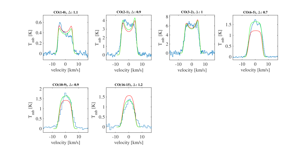
Figure 1: Best-fit CO models for R Dor. The blue histograms are the observations. The red lines are the model lines, the green lines are the model lines scaled to the same integrated intensities as the observations. The velocities are given with respect to the $\varv_{\rm{LSR}}$ = 6.5 km s^-1.

4.1 CO models

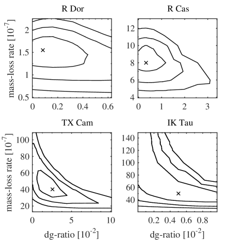
Figure 2: $\chi^{2}$-maps of the CO model grids for R Dor (top left), R Cas (top right), TX Cam (bottom left), and IK Tau (bottom right). The contours show the 1$\sigma$, 2$\sigma$, and 3$\sigma$ levels. The cross marks the lowest $\chi^{2}_{red}$ model.

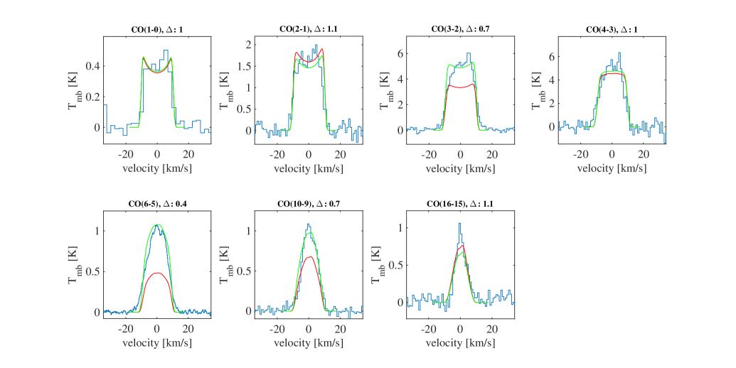
Figure 8: Best-fit CO models for R Cas. The blue histograms are the observations. The red lines are the model lines, the green lines are the model lines scaled to the same integrated intensities as the observations. The velocities are given with respect to the $\varv_{\rm{LSR}}$ = 24.5 km s^-1.

Figure 1 shows the best-fit CO models compared to the observed ground-based and HIFI lines for R Dor. Figures 8 to 10 show the equivalent for R Cas, TX Cam, and IK Tau, respectively. Table 3 gives the observed and modelled integrated intensities of all CO lines, including the PACS lines, together with the upper-level energies (E_up) and the ratios between models and observations for individual lines ($\Delta$). Fig. 2 shows the $\chi^{2}_{red}$ maps for the different CO model grids and Table 1 gives the best-fit parameters. The integrated intensities of the individual observed lines are all reproduced to within $\approx$25%. The average ratios between all observed and model lines ($\delta$) are all close to 1. Although observed by HIFI, the CO($16-15$) transition towards TX Cam is extremely over-estimated in the model by an order of magnitude, while the PACS line is well reproduced. The HIFI line is therefore excluded in the $\chi^{2}$ analysis. The ratio between modelled and observed line intensities as a function of $E_{\rm{up}}$ is shown in Fig. 3 (red crosses). Generally the lines scatter around a ratio of one, although there might be a slight correlation, with models preferentially under-predicting the intensities for low-$E_{\rm{up}}$ transitions.

For all models we use the photodissociation radius described by Mamon et al. (1988). This generally leads to overly resolved model line-profiles for the lower transitions, as evidenced by the double-peaked model line-profiles (specifically discussed for R Dor by Olofsson et al., 2002). This is a common problem in CO radiative-transfer models (e.g., Justtanont et al., 2005; Maercker et al., 2008; Danilovich et al., 2015). We attempted to fit the low-$J$ line profiles by reducing the CO envelope size. However, this generally leads to an underestimation of the total integrated intensity compared to the high-$J$ transitions. A possible way of correcting for this is by changing the dust parameters and the velocity field. However, the angular size of the envelope also depends on the assumed and uncertain distance to the source. Since this is a degenerate problem, we chose to fix the radius to the CO photodissociation radius and use the integrated intensities when determining the best-fit models.

In principle the terminal expansion velocity of the gas, $\upsilon_{g,\infty}$, should be well constrained by the width at zero power (in the following referred to as the width of the line) of the low-$J$ CO transitions, while the widths of the higher-$J$ CO transitions and H₂O transitions constrain the shape of the velocity profile ($\beta$ in Eq. 1). We attempt to constrain the velocity law using the observed CO and H₂O lines, adjusting $\beta$ in the radiative-transfer models to fit the observed line widths. For R Cas we derive $\beta=2.5$, and for the remaining three sources $\beta$=1.5. For IK Tau the momentum equation gives a steeper profile with $\beta=0.6$ (Decin et al., 2010c). Although comparatively shallow velocity profile seem to be preferred, the $\beta$ is not very well constrained by the observed CO and H₂O lines (Fig. 4), and we estimate the uncertainty in $\beta$ to be $\pm 1$.

The estimated mass-loss rates are consistent with previous estimates using the same radiative-transfer code and based on ground-based data alone (Maercker et al., 2008). Only for TX Cam do we derive a mass-loss rate a factor of $\approx$2 higher than the previous estimate $-$ still within the absolute uncertainty of independent mass-loss rate estimates of a factor of three (Ramstedt et al., 2008). The uncertainty in the mass-loss rate within the adopted model is $\approx$30%. For IK Tau it proved difficult to find an upper limit to the mass-loss rate, likely due to a saturation effect of the CO lines at high mass-loss rates, caused by increasing line optical depths and cooler envelopes (Ramstedt et al., 2008). See Sect. 5.5 for a comparison with similar codes.

The derived dust-to-gas ratios have considerable uncertainties. For R Dor and R Cas we derive values of a few times $10^{-4}$ with relatively strong constraints on the upper limit. For TX Cam we derive a value a factor $\approx$50 larger. For IK Tau the best-fit value is $\approx$10 times larger than for R Dor and R Cas, and agrees with chemical models at 6 R_∗ (Gobrecht et al., 2016), however no limits can be set. Ramstedt et al. (2008) derive values of a few times $10^{-3}$. The dust-to-gas ratio mainly affects the energy balance, where it is part of the heating of the gas through dust-gas collisions. This heating term depends degenerately also on the grain size and density. For this reason Schöier & Olofsson (2001) chose to combine these parameters in the so-called h-parameter. The derived d/g-ratios give h-parameters of 0.05, 0.03, 1.7, and 0.3 for R Dor, R Cas, TX Cam, and IK Tau, respectively. Ramstedt et al. (2008) derive values of 1.0 and 0.3 for TX Cam and IK Tau, respectively.

Finally, the kinetic temperature profiles are shown in Fig. 5. Note again that although the energy balance is solved in the CO models, the contribution from H₂O line cooling is not included in any of the models (see Sect. 3.3). For TX Cam, R Cas, and R Dor the profiles can be described well by power laws of the form

$$T(r)=T_{i}\times\left({\frac{r}{R_{i}}}\right)^{\alpha},$$ (6)

where $T_{i}$ is the temperature at the inner radius $R_{i}$. The exponents $\alpha$ are between $-0.6$ and $-1.0$. For the low mass-loss-rate M-type AGB star W Hya Khouri et al. (2014a) derive an exponent of $-0.65\pm 0.05$. In models of the chemical network in the CSE of AGB stars, Willacy & Millar (1997) use $\alpha$ = $-0.6$ for R Dor, TX Cam, and IK Tau.

Our profile for IK Tau deviates more from a simple power law in the inner and outermost parts of the CSE, but can generally be fit with $\alpha$ = $-0.98$. Solving the energy balance including H₂O line cooling in the modelling of CO lines towards IK Tau, Decin et al. (2010b) derive a temperature profile consistent with an exponent of $-0.6$, significantly different from our value. Their derived mass-loss rate is $\approx$50% higher than our value, and they use a dust-to-gas ratio a factor four higher. These values lie within the uncertainties quoted here and in Decin et al. (2010b), and it is not clear why there is a difference in temperature profile and whether this is related to the H₂O line cooling.

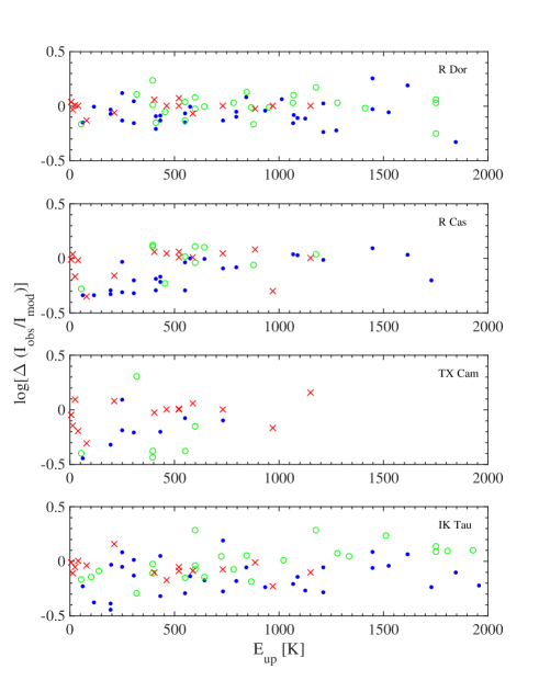
Figure 3: Ratio between observed and modelled integrated intensities vs. upper-level energy for the different transitions (CO: red crosses, ortho-H₂O: blue dots, para-H₂O: green circles).

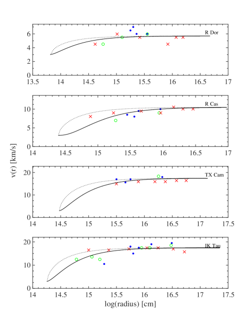
Figure 4: Velocity profiles derived for R Dor, R Cas, TX Cam and IK Tau (top to bottom) compared to the measured line-widths from lines emitted at different radii in the CSE (CO: red crosses, ortho-H₂O: blue dots, para-H₂O: green circles. The widths are measured at zero power. The radii are determined by the peak in the brightness profiles of each transition). The solid black lines give the profiles with the $\beta$ given in Table 1, the dotted black lines give the profile for $\beta=0.6$.

Table 1: Stellar parameters and results of the SED and CO line-emission models. T_∗ and L_∗ are the stellar effective temperature and luminosity, respectively. $R_{i}$ is the inner radius from which the CSE is modelled, and $T_{i}$ the temperature at the inner radius. $D$ is the distance to the source. $\tau_{\rm{d}}$ is the dust optical depth at 10 $\mu$m, $\upsilon_{\infty}$ the terminal gas expansion velocity, $\beta$ the exponent of the velocity law, d/g the derived dust-to-gas ratio, $\dot{M}$ the gas mass-loss rate, $R_{\rm{e}}$ the CO-photodissociation radius, $\delta$ the average ratio between integrated model and observed line intensities, and $\chi^{2}_{red}$ the reduced $\chi^{2}$ value of the best-fit model.

Source	$T_{*}$	$L_{*}$	$R_{i}$	$T_{i}$	$D$	$\tau_{d}$	$\upsilon_{\rm{\infty}}$	$\beta$	d/g	$\dot{M}$	$R_{\rm{e}}$	$\delta$	$\chi^{2}_{red}$
	[K]	[L⊙]	[$10^{13}$ cm]	[K]	[pc]		[km/s]		[$10^{-2}$]	[$10^{-7}$ M⊙]	[$10^{16}$ cm]
R Dor	2400	6500	6.6	1680	59	0.05	5.7	1.5	0.08	1.6	1.6	1.0	0.65
R Cas	1800	8725	25	1050	172	0.09	10.5	2.5	0.04	8.0	3.2	0.9	1.7
TX Cam	2400	8600	30	845	380	0.4	17.5	1.5	2.6	40	6.6	0.9	3.1
IK Tau	2100	7700	18	960	265	1.0	17.5	1.5	0.5	50	7.5	0.9	2.9

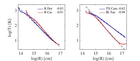
Figure 5: Kinetic temperature profiles (solid lines) calculated in the energy balance of the CO modelling for R Dor (left panel, blue), R Cas (left panel, red), TX Cam (right panel, blue), and IK Tau (right panel, red). The dashed lines show power-law fits to the individual profiles (Eq. 6). The numbers give the exponents for the respective fits.

4.2 H₂O models

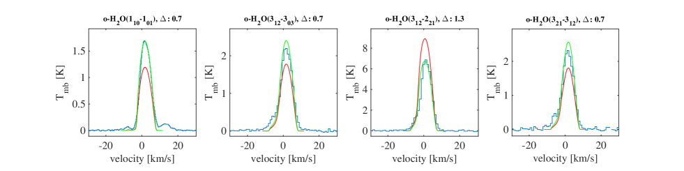
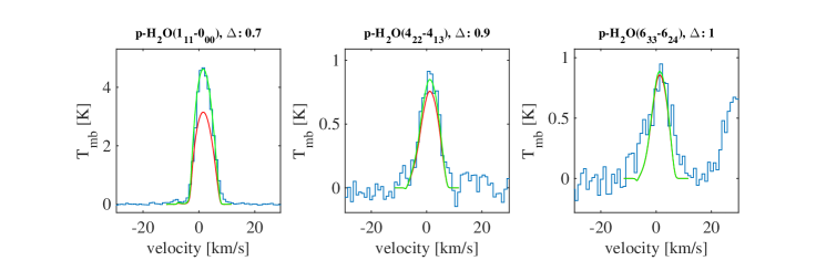
Figure 6: Best-fit o-H₂O and p-H₂O models of the HIFI Lines for R Dor. The blue histograms are the observations. The red lines are the model lines, the green lines are the model lines scaled to the same integrated intensities as the observations. The velocities are given with respect to the $\varv_{\rm{LSR}}$ = 6.5 km s^-1.

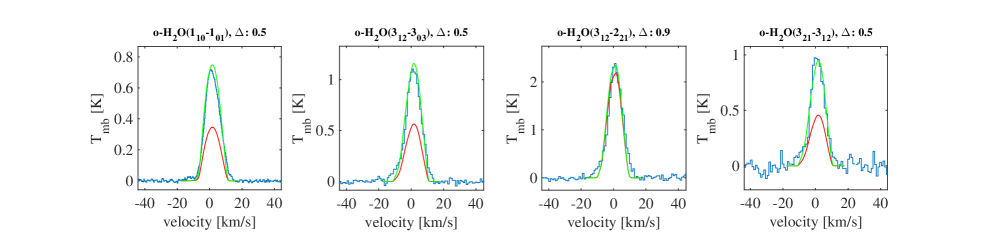
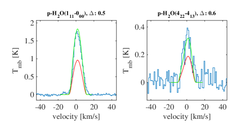
Figure 11: Best-fit o-H₂O and p-H₂O models of the HIFI Lines for R Cas. The blue histograms are the observations. The red lines are the model lines, the green lines are the model lines scaled to the same integrated intensities as the observations. The velocities are given with respect to the $\varv_{\rm{LSR}}$ = 24.5 km s^-1.

Figure 6 shows the best-fit ortho-H₂O and para-H₂O models for the HIFI lines compared to the observed lines for R Dor. Figures 11 to 13 show the equivalent for R Cas, TX Cam, and IK Tau, respectively. Tables 4 and 5 list the same parameters as Table 3, but for the HIFI and PACS lines of ortho-H₂O and para-H₂O, respectively. Figure 7 shows the $\chi^{2}_{red}$-maps for ortho-H₂O and para-H₂O for all objects. We indicate both the best-fit radius in the grid, as well as the best-fit H₂O abundance using the radius determined by Netzer & Knapp (1987), $R_{\rm{NK}}$. It is not possible to set upper limits to the H₂O radii. The H₂O line emitting region is limited by radiative excitation, and the H₂O lines hence do not probe the outer regions very well. In all cases $R_{\rm{NK}}$ is consistent with the best-fit radius when allowing $R$ to vary freely, and we use this radius for the H₂O envelope. All model results refer to models using $R_{\rm{NK}}$. Table 2 gives the best-fit values for the abundance, the average ratios between all integrated model and observed line intensities ($\delta$), and the $\chi^{2}_{red}$ values. The dependence of the model and observed line ratios on the upper level energy $E_{\rm{up}}$ is shown in Fig. 3. As with the CO lines, the scatter lies around one, with a slight under-prediction by the model lines. However, no clear trend with $E_{\rm{up}}$ can be seen.

The derived ortho-H₂O abundances lie between $\approx$$10^{-5}$–$10^{-4}$ relative to H₂. For R Dor and R Cas this is significantly lower than previously derived values based only on ISO observations (Maercker et al., 2008). Including the spectrally resolved 557 GHz line observed with Odin required a reduction of the (constant) expansion velocity to fit the observed line-width, and led to a slight reduction in the ortho-H₂O abundance for R Dor, albeit well within the uncertainties (Maercker et al., 2009). Including a velocity profile forces a significant reduction of the H₂O abundance to reproduce the observed intensities. Observations of several para-H₂O lines allow us to set constraints on the para-H₂O abundances and derive ortho/para-H₂O ratios (o/p-ratio). The uncertainties in the derived abundances lead to considerable uncertainties in the derived o/p-ratios. This is especially true for TX Cam, where the low number of observed para-H₂O lines leads to a bad fit to the observations with the by-far highest $\chi^{2}_{red}$ value.

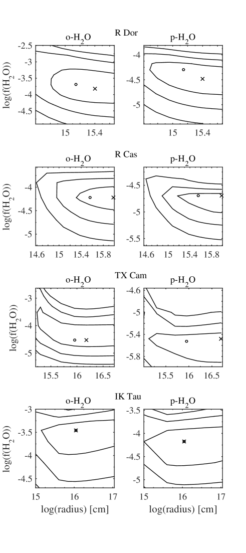
Figure 7: $\chi^{2}$-maps of the o-H₂O (left) and p-H₂O (right) model grids for R Dor , R Cas , TX Cam , and IK Tau (top to bottom). The cross marks the best-fit model using the H₂O radius as a free parameter, the circle the best-fit model using R_NK.

Table 2: Results of the H₂O modelling. The H₂O abundances are given relative to H₂. The values in brackets give the 1$\sigma$ ranges.

Source	$R_{\rm{NK}}$	f(o-H2O)	$\delta$	$\chi^{2}_{red}$	f(p-H2O)	$\delta$	$\chi^{2}_{red}$	o/p-ratio
	[$\times 10^{15}$ cm]	[$\times 10^{-4}$]			[$\times 10^{-4}$]
R Dor	1.4	2 (0.7 – 5.6)	0.9	1.11	0.5 (0.2 – 0.7)	1.0	1.0	4 (1 – 26)
R Cas	3.6	0.6 (0.4 – 0.9)	0.8	1.9	0.2 (0.1 – 0.3)	1.0	1.6	3 (1 –9)
TX Cam	9.0	0.3 (0.2 – 1.0)	0.6	3.9	0.03 (0.01 – 0.04)	0.7	6.7	10 (5 – 100)
IK Tau	11	3.5 (1.1 – 5)	0.8	1.8	0.7 (0.2 – 1.3)	0.9	1.2	5 (0.8 – 25)

5 Discussion

5.1 The significance of H₂O line cooling

The current implementation of H₂O line cooling in the radiative-transfer codes implies that line cooling by H₂O significantly affects the temperature in the inner envelope of M-type AGB stars (at radii $R_{\rm{i}}<r<$ a few $R_{\rm{i}}$). The energy balance in this inner part of the CSE is very sensitive to the amount of H₂O line cooling included in the model, quickly leading to extreme cooling. Models of the S-type stars $\chi$ Cyg and W Aql, that include H₂O line cooling, had H₂O abundances factors $2-35$ lower than the abundances estimated for the M-type stars here (Schöier et al., 2011; Danilovich et al., 2014). For our high mass-loss-rate objects, H₂O line cooling is too strong to be included in the energy balance. For R Dor and R Cas we nevertheless managed to include 100% H₂O line cooling. While the iterative procedure does not allow us to realistically calculate a grid of models due to computational limitations, the resulting fit to the observed lines gives similar $\chi^{2}_{red}$ values to the models without H₂O line cooling. The derived mass-loss rates and H₂O abundances do not change significantly between models with and without cooling, since the observed CO lines effectively constrain the temperature profile. However, to balance the additional cooling in the inner envelope the d/g ratio needs to be increased by a factor of approximately two. Much more importantly, the only way we managed to include full H₂O line cooling was to change the drift-velocity profile from starting low and increasing with radius to starting high and decreasing with radius. This changes the dust-velocity profile to a constant value throughout the entire CSE. Although the dust velocity profile and the drift velocity are not constrained observationally, theoretical models of dust-driven winds generally predict very low drift velocities between the dust and the gas for high mass-loss rates, and increasing drift-velocity with increasing distance (as assumed in this paper), or a constant drift velocity. A situation where the dust velocity is constant throughout the envelope therefore seems unphysical.

A constant dust velocity drastically increases the heating due to the dust-gas interaction in the inner CSE, and hence balances the cooling due to H₂O. While this scenario is unrealistic, it indicates that some physics leading to heating in the inner envelope may be missing. Since the dust-velocity profile is not constrained by observations, changing the profile in an ad hoc manner becomes similar to adding an arbitrary heating term to counter-balance the cooling by H₂O. We have no suggestion as to what this additional heating may be, or whether this indicates a fundamental problem in our understanding of the physics in the inner CSEs of AGB stars.

Another possible explanation for the problem of extreme H₂O line cooling is the way the line cooling is calculated. In the current version of the radiative transfer, the contribution due to line cooling (for any molecule) is included following Sahai (1990):

$$C_{line}(r)=\sum_{l,u>l}\Delta E_{ul}k_{B}(p_{l}c_{lu}-p_{u}c_{ul}),$$ (7)

where $\Delta E_{ul}$ is the energy difference of a transition from upper level $u$ to lower level $l$, $k_{B}$ the Boltzmann constant, $p_{l}$ and $p_{u}$ the lower and upper level population densities, and $c_{lu}$ and $c_{ul}$ the collisional excitation and de-excitation rates from the lower to upper and upper to lower levels, respectively. If the total sum is positive, the rate of downward collisions is lower than the rate of upward collisions. The difference in energy is assumed to be radiated away, leading to net cooling. The contribution to the cooling is calculated in each radial bin. While this approach may be valid for lines that are optically thin throughout the CSE, the fact that no description of the optical depth is included may be problematic at the very high optical depths of the majority of the H₂O-transitions. The net cooling assumes that the lost energy leaves the radial bin (and CSE). For very high optical depths, however, the radiated energy may be re-absorbed – either in a radial bin further out, or possibly still in the same radial bin. This would feed energy back into the envelope and reduce the net cooling. The current implementation may hence overestimate the amount of line cooling from H₂O.

This problem could possibly be solved by simply scaling the contribution to the cooling in Eq. 7 by the escape probability $(1-e^{-\tau})/\tau$. The implementation of this in the code is however not trivial. The optical depth depends on the direction and is affected by the surrounding density and velocity profiles. Since the code only works along the radial direction, an angle-averaged optical depth $\bar{\tau}$ would have to be calculated at each radial point, which is not straight-forward. We are currently working on this problem, trying to address the issue of properly including radiative line cooling into the code.

Note that this does not only affect the cooling due to H₂O. In principle CO can also reach high optical depths, and in carbon AGB stars cooling due to HCN lines affect the temperature structure in the inner CSE in a very similar way to H₂O in M-type AGB stars. Including line cooling correctly in the radiative-transfer codes, and identifying any potentially missed heating (or cooling mechanisms) is essential for a complete understanding of the physical conditions in the inner CSEs of AGB stars. This in turn affects chemical and dynamical models of the inner winds, and our understanding of the evolution of the star on the AGB in general.

5.2 The velocity profiles

Although not very well constrained, we derive comparatively shallow velocity profiles for all sources, with $\beta=1.5\pm 1.0$. For IK Tau, Decin et al. (2010c) derive a $\beta=1-1.8$. The velocity profiles derived here and by Decin et al. (2010c) are consistent with measurements of maser lines in the CSE of IK Tau (Bains et al., 2003). The momentum equation for IK Tau on the other hand gives $\beta=0.6$ (Decin et al., 2010c). Khouri et al. (2014a) adopt a $\beta=1.5$ to describe the velocity profile in W Hya, and find evidence that higher values may fit the high-$J$ transitions of CO better. Note that using the upper-state energy $\rm{E_{up}}$ as a measure of the distance in the CSE and the line width to constrain the velocity profile as done by Justtanont et al. (2012) can be misleading. For R Dor the measured line width vs. $\rm{E_{up}}$ for all molecules detected in the HIFISTARS observations implies that R Dor has a decelerating wind (Justtanont et al., 2012), showing the importance of using full radiative transfer in order to derive correct velocity profiles.

All measurements indicate that the wind follows a more shallow profile than generally predicted by dynamical models solving the coupled momentum equations of the dust and gas (e.g., Decin et al., 2006; Ramstedt et al., 2008; Decin et al., 2010c). Note however, that Ramstedt et al. (2008) derive a velocity profile for IK Tau that is consistent with the results by Bains et al. (2003), showing that it is possible to derive velocity profiles from dynamical models that are consistent with the observed, shallow profiles. At the same time this shows the large uncertainty in the dynamical models, likely due to a sensitive dependence on the input parameters, and the assumption of a fully momentum coupled wind. The choice of $\upsilon_{\rm{g,i}}$ does not significantly affect our results. The observed lines are emitted from too far out in the wind to effectively constrain the wind velocity at the inner radius. Any reasonable changes in $\upsilon_{\rm{g,i}}$ would not change the derived $\beta$ values, but would mainly affect the energy balance in the inner CSE. However, compared to the uncertainty in the treatment of the line cooling, this effect is small.

5.3 H₂O abundances

For all sources we derive total H₂O abundances between $(0.3--4.0)\times 10^{-4}$ relative to H₂ (at the inner radius of our model CSE, i.e. $R_{i}$). Previous modelling of ISO observations of o-H₂O resulted in the same o-H₂O abundances for R Dor and IK Tau, while the values for R Cas and TX Cam were factors 5 and 10 higher, respectively. For IK Tau, Decin et al. (2010c) derive a total H₂O abundance of $6.6\times 10^{-5}$, uncertain by a factor of 2. Within our uncertainties we just manage to meet the value derived by Decin et al. (2010c). However, they use a mass-loss rate that is higher by $\approx$50% than our value, likely resulting in a lower H₂O abundance. For the M-type AGB star W Hya, previously derived H₂O abundances are $8\times 10^{-4}$ and $3\times 10^{-4}$ (at radii smaller and larger than $4.5\times 10^{14}$ cm, respectively; Barlow et al., 1996) ,and $9\times 10^{-4}$ (Khouri et al., 2014b). For non-LTE chemical models, the predicted H₂O abundance in the inner CSE ($<5\,R_{*}$) of M-type AGB stars is $4\times 10^{-4}$ relative to H₂, while LTE models predict H₂O abundances closer to $7\times 10^{-5}$ (using TX Cam as an example; Cherchneff, 2006). Non-LTE chemical models of IK Tau predict H₂O abundances of $\approx 2\times 10^{-4}$ at 6 R_∗ (Gobrecht et al., 2016), consistent with our value derived here. Although the H₂O abundances derived here and in other publications based on radiative-transfer modelling cover a large range, values of a few times $10^{-4}$ appear to be an upper limit. Taken at face value, and assuming that H₂O abundances remain largely unaffected by processes in the intermediate wind, the results here favour the formation of H₂O under non-LTE conditions in the inner wind. However, within the uncertainties, the derived abundances seem also to be consistent with the formation of H₂O under equilibrium conditions at $1\,R_{*}$. The derived ortho- to para-H₂O ratio is very uncertain, but is generally consistent with a value of 3, implying formation of H₂O under warm conditions.

5.4 Discrepancies between models and observations

Although the 1D radiative-transfer models generally reproduce the overall line shapes (line-width and double-peaked, flat-topped, parabolic, or triangular lines), it is clear that deviations from these simple profiles are not reproduced. In addition to over-resolved low-$J$ lines in CO, asymmetries between the red- and blue-shifted sides of the lines, and bumps and additional peaks (e.g. in R Dor and R Cas, CO($6-5$) at $\approx$3km s^-1), are not reproduced. In the H₂O lines the self-absorption on the blue side due to the high optical depths of the lines is generally well reproduced, however also with some deviations.

These differences may be caused by several effects. Varying mass-loss rates, velocity profiles, and photodissociation efficiencies will affect the spatial density distribution of the circumstellar wind, and the fractional abundance distribution of the molecules. This will change the optical depths of the lines and the excitation conditions. Such effects could, in principle, be included in the 1D radiative transfer. However, effects due to the three dimensional structure may have an equal, or even stronger, effect on the observed lines. These include asymmetric winds, disks and tori, and clumpiness of the circumstellar matter. Shocks in the inner wind and asymmetric illumination of the CSE due to convection cells on the stellar surface and atmospheric molecular absorption bands can also strongly affect the observed line shapes. Since the beginning of science observations with ALMA (Atacama Large Millimeter/submillimeter Array), an increasingly complex picture of the inner winds of AGB stars is being established, including the effects mentioned above. VLT-SPHERE observations in the optical of R Dor resolve the stellar disk, and show clear signs of an irregular brightness distribution from the stellar surface due to convection cells (Khouri et al. in preparation).

5.5 Comparison to radiative transfer with GASTRoNOoM

Solving the molecular line radiative transfer for CSEs around AGB stars encounters several physical (e.g. energy balance, radiation fields, velocity profiles, molecular data) and numerical (e.g. modelling strategies, matrix inversion, optical depths) problems that have to be solved. As such, the number of advanced, non-LTE radiative-transfer codes in use is limited. This is unfortunate, since this makes benchmarking, and comparison and verification of model results difficult. One of the radiative-transfer codes that approaches the modelling of AGB CSEs in a similar way to our code is GASTRoNOoM (Decin et al., 2006, 2007, 2008).

The estimate of the mass-loss rate for IK Tau based on GASTRoNOoM lies within 50% of our results (Decin et al., 2010c). Khouri et al. (2014a) derive a mass-loss rate for W Hya of $1.5\times 10^{-7}$ $M_{\odot}$ yr^-1, compared to $1.0\times 10^{-7}$ $M_{\odot}$ yr^-1 in our previous modelling (Maercker et al., 2008). Based on a grid of models using GASTRoNOoM, De Beck et al. (2010) derive a formula to estimate the mass-loss rates from AGB stars based on the intensities of the CO lines. Using their formula results in mass-loss rates that are less than a factor two different from the values derived here. This is well within the limit of the absolute uncertainty expected from this modelling method (Ramstedt et al., 2008). Compared to what we find in our modelling, the derived H₂O abundances using GASTRoNOoM appear to be lower by a factor of two for IK Tau. Comparing the results by Khouri et al. (2014b) with Maercker et al. (2008), they are a factor of five lower for W Hya. However, the absolute uncertainties are relatively large, and a more systematic comparison between the two radiative-transfer codes is necessary to identify whether the discrepancy in H₂O abundances is due to numerical differences in the codes, or simply reflects the uncertainty and difficulty in modelling H₂O line emission.

6 Conclusions

We have successfully modelled CO and H₂O lines observed towards four M-type AGB stars, including spectrally resolved ground-based and HIFI observations for CO, spectrally resolved HIFI observations of o-H₂O and p-H₂O, and spectrally unresolved observations of CO and H₂O with PACS. These are the first models of a larger sample of sources with spectrally resolved H₂O line profiles. We derive H₂O abundances, o/p-H₂O ratios, the sizes of the H₂O line emitting regions, velocity and temperature profiles, and attempt to include full H₂O line cooling in the energy balance in the radiative transfer. Based on the modelling we arrive at following conclusions.

• Our modelling indicates that the winds around these four M-type AGB stars have a comparatively shallow acceleration profile, in contrast to what is generally expected from dynamical models of dust-driven winds. However, we also note that the widths of the line profiles only moderately constrain the velocity profile.

• Although we managed to include H₂O line cooling in the energy balance for the low mass-loss rate objects R Dor and R Cas, this required an unphysical description of the dust expansion velocity in order to counter-balance the extreme cooling from H₂O in the inner CSE. This implies that the physical processes that describe the heating and cooling in the inner envelope are not completely understood and/or that the formal implementation of line cooling is not correct.

• We derive generally high H₂O abundances, up to a few times $10^{-4}$ relative to H₂. Within the uncertainties, all derived abundances are consistent with both NLTE and LTE abundances derived from chemical models, emphasizing the importance of improved radiative transfer models to reduce uncertainties on abundances derived from observations.

• The derived o/p-ratios are uncertain, however consistent with a value of three, indicating formation of H₂O in the warm, inner CSE.

Computational limitations currently do not allow us to self-consistently solve the physics and dynamics throughout the CSE in three dimensions. 1D radiative-transfer models as presented here are important for constraining the basic physical parameters of the envelopes (e.g., temperature, velocity, average mass-loss rates). These can be used as input for 3D models  (e.g. LIME; Brinch & Hogerheijde, 2010) to study the effect of structure in three dimensions. In order to arrive at a self-consistent model that fully describes the physical conditions throughout the CSE, however, it is important to solve the problem of radiative line cooling, in particular for H₂O.

Appendix A Observed and model line intensities, and model line profiles

Table 3: Observed and modelled CO lines.

				R Dor				R Cas				TX Cam				IK Tau
Transition	$\lambda$	Eup		Iobs	Imod	$\Delta$		Iobs	Imod	$\Delta$		Iobs	Imod	$\Delta$		Iobs	Imod	$\Delta$
$J$-level	[GHz]	[K]		[K km s-1 ]				[K km s-1 ]				[K km s-1 ]				[K km s-1 ]
Ground based
CO$(1-0)$	115.3	3.85		5.00	5.52	1.10		8.40	8.21	0.98		14.5	13.0	0.90		33.0	32.0	0.97
CO$(2-1)$	230.5	11.54		41.6	38.5	0.93		32.1	35.1	1.09		60.6	43.7	0.72		95.0	74.1	0.78
CO$(3-2)$	345.8	23.07		70.4	72.4	1.03		100	68.3	0.68		70.0	87.4	1.25		125	110	0.88
CO$(4-3)$	461.0	38.45		–	–	–		89.6	85.7	0.96		149	95.7	0.64		130	130	1.00
$J$-level	[GHz]	[K]		[K km s-1 ]				[K km s-1 ]				[K km s-1 ]				[K km s-1 ]
HIFI
CO$(6-5)$	691.5	80.74		16.8	12.5	0.74		17.2	7.74	0.45		16.6	8.19	0.49		12.0	10.9	0.91
CO$(10-9)$	1152.0	211.40		15.9	13.8	0.87		12.8	8.87	0.69		8.15	9.86	1.21		9.45	13.7	1.45
CO$(16-15)$	1841.3	522.48		11.6	13.8	1.19		6.76	7.69	1.14		–	–	–		15.9	14.1	0.89
$J$-level	[$\mu$m]	[K]		[$10^{-16}$ W m-2]				[$10^{-16}$ W m-2]				[$10^{-16}$ W m-2]				[$10^{-16}$ W m-2]
PACS
CO$(14-13)$	186.00	403.46		2.43	2.78	1.14		1.45	1.65	1.14		2.06	1.96	0.95		3.63	2.85	0.79
CO$(15-14)$	173.63	461.05		2.94	2.96	1.01		1.53	1.70	1.11		2.07	2.06	1.00		4.55	3.03	0.67
CO$(16-15)$	162.81	522.48		–	–	–		1.70	1.74	1.02		2.07	2.14	1.03		3.93	3.18	0.81
CO$(17-16)$	153.27	587.72		3.77	3.26	0.86		1.70	1.75	1.03		1.93	2.20	1.14		4.06	3.30	0.81
CO$(19-18)$	137.20	729.68		–	–	–		1.55	1.72	1.11		–	–	–		4.06	3.44	0.85
CO$(21-20)$	124.19	886.90		3.77	3.55	0.94		1.35	1.63	1.21		8.77	2.21	0.25		3.53	3.46	0.98
CO$(22-21)$	118.58	971.23		–	–	–		3.16	1.57	0.50		3.18	2.17	0.68		5.79	3.42	0.59
CO$(24-23)$	108.76	1151.32		–	–	–		–	–	–		1.40	2.03	1.45		4.16	3.27	0.79

Table 4: Observed and modelled ortho-H₂O lines.

				R Dor				R Cas				TX Cam				IK Tau
Transition	$\lambda$	Eup		Iobs	Imod	$\Delta$		Iobs	Imod	$\Delta$		Iobs	Imod	$\Delta$		Iobs	Imod	$\Delta$
$J_{\mathrm{K}_{\mathrm{a}},\mathrm{K}_{\mathrm{c}}}$-level	[GHz]	[K]		[K km s-1 ]				[K km s-1 ]				[K km s-1 ]				[K km s-1 ]
HIFI
o-H2O $(1_{10}-1_{01})$	556.9	60.96		12.3	8.72	0.71		8.36	3.87	0.46		6.71	2.45	0.36		11.4	6.8	0.59
o-H2O $(5_{32}-4_{41})$	620.7	732.06		–	–	–		–	–	–		–	–	–		18.2	28.2	1.55
o-H2O $(3_{12}-3_{03})$	1097.4	249.43		18.6	13.7	0.74		13.1	6.36	0.49		7.24	4.68	0.65		15.7	14.1	0.89
o-H2O $(3_{12}-2_{21})$	1153.1	249.43		51.6	68.3	1.32		24.9	23.1	0.93		10.6	13.2	1.24		28.4	34.4	1.21
o-H2O $(3_{21}-3_{12})$	1162.9	305.24		19.3	13.6	0.70		10.4	5.02	0.48		4.91	3.07	0.62		15.1	11.2	0.74
o-H2O $(3_{02}-2_{12})$	1716.8	196.77		–	–	–		–	–	–		–	–	–		32.2	30.1	0.93
$J_{\mathrm{K}_{\mathrm{a}},\mathrm{K}_{\mathrm{c}}}$-level	[$\mu$m]	[K]		[$10^{-16}$ W m-2]				[$10^{-16}$ W m-2]				[$10^{-16}$ W m-2]				[$10^{-16}$ W m-2]
PACS
o-H2O $(2_{21}-2_{12})$	180.49	194.09		5.92	5.51	0.93		2.65	1.25	0.47		3.77	1.00	0.27		5.93	2.14	0.36
o-H2O $(2_{12}-1_{01})$	179.53	114.38		14.3	14.1	0.99		7.32	3.39	0.46		8.56	2.56	0.30		10.0	4.18	0.42
o-H2O $(7_{34}-7_{25})$	166.81	1211.96		2.32	1.35	0.58		0.33	0.32	0.97		–	–	–		2.52	1.31	0.52
o-H2O $(5_{32}-5_{23})$	160.51	732.06		4.27	3.16	0.74		1.07	0.86	0.81		0.79	0.63	0.80		4.20	2.21	0.53
o-H2O $(8_{45}-7_{52})$	159.05	1615.32		4.87	7.54	1.55		0.56	0.61	1.08		–	–	–		1.94	2.25	1.16
o-H2O $(5_{14}-5_{05})$	134.94	574.73		6.48	6.38	0.99		1.71	1.70	1.00		–	–	–		6.37	4.65	0.73
o-H2O $(8_{36}-7_{43})$	133.55	1447.57		10.1	18.2	1.80		–	–	–		–	–	–		4.45	5.44	1.22
o-H2O $(4_{23}-4_{14})$	132.41	432.15		9.88	8.10	0.82		3.28	2.01	0.61		2.51	1.58	0.63		9.47	4.59	0.48
o-H2O $(9_{45}-9_{36})$	129.34	1957.06		–	–	–		–	–	–		–	–	–		2.61	1.56	0.60
o-H2O $(7_{25}-7_{16})$	127.88	1125.71		3.07	2.35	0.77		–	–	–		–	–	–		5.82	3.16	0.54
o-H2O $(9_{36}-9_{27})$	123.46	1845.82		2.72	1.29	0.47		–	–	–		–	–	–		2.23	1.75	0.79
o-H2O $(4_{32}-4_{23})$	121.72	550.35		9.33	6.65	0.71		3.17	1.61	0.51		1.60	1.34	0.84		9.86	5.00	0.51
o-H2O $(7_{34}-6_{43})$	116.78	1211.96		15.7	16.7	1.06		–	–	–		–	–	–		7.48	6.56	0.88
o-H2O $(2_{21}-1_{10})$	108.07	194.09		32.7	27.8	0.85		13.3	6.76	0.51		10.2	4.94	0.48		24.5	10.2	0.41
o-H2O $(6_{34}-6_{25})$	104.09	933.73		5.96	5.43	0.91		–	–	–		–	–	–		10.8	6.23	0.58
o-H2O $(6_{25}-6_{16})$	94.64	795.51		11.3	8.99	0.80		3.05	2.52	0.83		–	–	–		12.4	8.22	0.66
o-H2O $(6_{43}-6_{34})$	92.81	1088.75		8.60	6.68	0.78		1.60	1.72	1.07		–	–	–		10.3	7.40	0.72
o-H2O $(8_{36}-8_{27})$	82.98	1447.57		5.74	5.42	0.94		1.16	1.44	1.24		–	–	–		9.33	8.08	0.87
o-H2O $(6_{16}-5_{05})$	82.03	643.49		–	–	–		9.97	9.85	0.99		–	–	–		9.44	6.35	0.67
o-H2O $(9_{27}-9_{18})$	81.41	1729.29		–	–	–		1.65	1.04	0.63		–	–	–		29.8	17.4	0.58
o-H2O $(4_{23}-3_{12})$	78.74	432.15		50.4	37.1	0.74		16.3	11.0	0.68		–	–	–		7.19	8.07	1.12
o-H2O $(7_{52}-7_{43})$	77.76	1524.86		6.16	5.42	0.88		–	–	–		–	–	–		11.4	10.4	0.91
o-H2O $(5_{50}-5_{41})$	75.91	1067.68		13.7	9.65	0.70		1.99	2.16	1.09		–	–	–		36.6	22.6	0.62
o-H2O $(3_{21}-2_{12})$	75.38	305.24		51.4	57.2	1.11		20.9	13.2	0.63		–	–	–		18.0	18.5	1.03
o-H2O $(7_{07}-6_{16})$	71.95	843.47		30.4	36.9	1.21		–	–	–		–	–	–		14.7	12.9	0.88
o-H2O $(8_{27}-8_{18})$	70.70	1274.17		19.0	11.4	0.60		–	–	–		–	–	–		–	–	–
o-H2O $(3_{30}-3_{03})$	67.27	410.65		51.9	32.0	0.62		13.8	7.05	0.51		–	–	–		–	–	–
o-H2O $(3_{30}-2_{21})$	66.44	410.65		62.8	50.6	0.81		17.8	11.6	0.65		–	–	–		–	–	–
o-H2O $(7_{16}-6_{25})$	66.09	1013.20		42.1	48.6	1.16		–	–	–		–	–	–		–	–	–
o-H2O $(6_{25}-5_{14})$	65.17	795.51		40.7	36.3	0.89		–	–	–		–	–	–		–	–	–
o-H2O $(8_{18}-7_{07})$	63.32	1070.68		52.0	42.9	0.83		–	–	–		–	–	–		–	–	–
o-H2O $(4_{32}-3_{21})$	58.70	550.35		54.3	46.5	0.86		14.2	13.1	0.92		–	–	–		–	–	–

Table 5: Observed and modelled para-H₂O lines.

				R Dor				R Cas				TX Cam				IK Tau
Transition	$\lambda$	Eup		Iobs	Imod	$\Delta$		Iobs	Imod	$\Delta$		Iobs	Imod	$\Delta$		Iobs	Imod	$\Delta$
$J_{\mathrm{K}_{\mathrm{a}},\mathrm{K}_{\mathrm{c}}}$-level	[GHz]	[K]		[K km s-1 ]				[K km s-1 ]				[K km s-1 ]				[K km s-1 ]
HIFI
p-H2O $(2_{11}-2_{02})$	752.0	136.94		–	–	–		–	–	–		–	–	–		13.2	10.9	0.82
p-H2O $(5_{24}-4_{31})$	970.3	598.83		–	–	–		–	–	–		–	–	–		17.5	33.7	1.93
p-H2O $(2_{02}-1_{11})$	987.9	100.84		–	–	–		–	–	–		–	–	–		23.7	17.0	0.72
p-H2O $(1_{11}-0_{00})$	1113.3	53.54		33.6	22.9	0.68		19.8	10.4	0.53		13.2	5.31	0.40		24.4	16.5	0.68
p-H2O $(4_{22}-4_{13})$	1207.6	454.33		6.72	5.99	0.89		3.36	1.98	0.59		–	–	–		–	–	–
p-H2O $(5_{33}-6_{06})$	1717.0	725.09		–	–	–		–	–	–		–	–	–		2.70	3.01	1.11
p-H2O $(6_{33}-6_{24})$	1762.0	951.82		6.18	5.97	0.97		–	–	–		–	–	–		2.10	7.49	3.57
$J_{\mathrm{K}_{\mathrm{a}},\mathrm{K}_{\mathrm{c}}}$-level	[$\mu$m]	[K]		[$10^{-16}$ W m-2]				[$10^{-16}$ W m-2]				[$10^{-16}$ W m-2]				[$10^{-16}$ W m-2]
PACS
p-H2O $(4_{13}-4_{04})$	187.11	396.38		2.61	2.66	1.02		0.74	0.95	1.29		0.94	0.35	0.37		2.28	2.17	0.95
p-H2O $(7_{35}-6_{42})$	169.74	1175.03		2.74	4.05	1.48		0.53	0.58	1.10		–	–	–		1.66	3.21	1.93
p-H2O $(6_{24}-6_{15})$	167.03	867.25		1.08	1.05	0.97		–	–	–		–	–	–		2.64	1.72	0.65
p-H2O $(4_{31}-4_{22})$	146.92	552.26		3.34	3.66	1.10		1.05	1.09	1.04		0.82	0.34	0.42		4.20	2.93	0.70
p-H2O $(4_{13}-3_{22})$	144.52	396.38		11.6	19.8	1.71		3.22	4.29	1.33		2.63	1.11	0.42		8.46	6.62	0.78
p-H2O $(4_{04}-3_{13})$	125.35	319.48		20.2	25.9	1.28		–	–	–		0.88	1.78	2.03		15.0	7.59	0.51
p-H2O $(9_{37}-8_{44})$	118.41	1749.88		3.30	1.86	0.56		–	–	–		–	–	–		1.83	2.51	1.37
p-H2O $(9_{46}-8_{53})$	117.68	1929.22		–	–	–		–	–	–		–	–	–		1.53	1.95	1.27
p-H2O $(5_{24}-5_{15})$	111.63	598.83		6.18	5.82	0.94		1.92	1.77	0.92		0.97	0.68	0.70		7.28	6.12	0.84
p-H2O $(5_{42}-5_{33})$	94.21	877.81		7.38	5.01	0.68		1.49	1.29	0.87		–	–	–		–	–	–
p-H2O $(7_{44}-7_{35})$	90.05	1334.81		–	–	–		–	–	–		–	–	–		5.29	5.91	1.12
p-H2O $(6_{06}-5_{15})$	83.28	642.69		31.9	31.7	0.99		5.81	7.33	1.26		–	–	–		20.2	14.6	0.72
p-H2O $(8_{35}-7_{44})$	81.69	1510.93		–	–	–		–	–	–		–	–	–		4.79	82.4	1.72
p-H2O $(7_{26}-7_{17})$	81.22	1020.93		–	–	–		–	–	–		–	–	–		9.42	9.68	1.03
p-H2O $(8_{53}-8_{44})$	80.56	1806.97		–	–	–		–	–	–		–	–	–		4.60	5.76	1.25
p-H2O $(6_{15}-5_{24})$	78.93	781.12		29.1	31.5	1.08		–	–	–		–	–	–		19.8	16.7	0.84
p-H2O $(6_{51}-6_{42})$	76.42	1278.54		–	–	–		–	–	–		–	–	–		7.63	9.08	1.19
p-H2O $(9_{37}-9_{28})$	73.61	1749.88		–	–	–		–	–	–		–	–	–		5.54	6.74	1.22
p-H2O $(5_{51}-6_{24})$	71.79	1067.67		–	–	–		–	–	–		–	–	–		6.20	0.62	0.10
p-H2O $(7_{17}-6_{06})$	71.54	843.81		25.3	34.1	1.35		–	–	–		–	–	–		15.1	17.0	1.13
p-H2O $(5_{24}-4_{13})$	71.07	598.83		29.4	35.4	1.20		6.91	8.91	1.29		–	–	–
p-H2O $(3_{31}-2_{20})$	67.09	410.36		50.8	35.9	0.71		–	–	–		–	–	–		–	–	–
p-H2O $(8_{08}-7_{17})$	63.46	1070.54		24.8	31.5	1.27		–	–	–		–	–	–		–	–	–
p-H2O $(4_{31}-4_{04})$	61.81	552.26		25.8	19.1	0.74		–	–	–		–	–	–		–	–	–
p-H2O $(8_{26}-7_{35})$	60.16	1749.82		19.3	22.0	1.14		–	–	–		–	–	–		–	–	–
p-H2O $(7_{26}-6_{15})$	59.99	1414.18		31.7	30.5	0.96		–	–	–		–	–	–		–	–	–

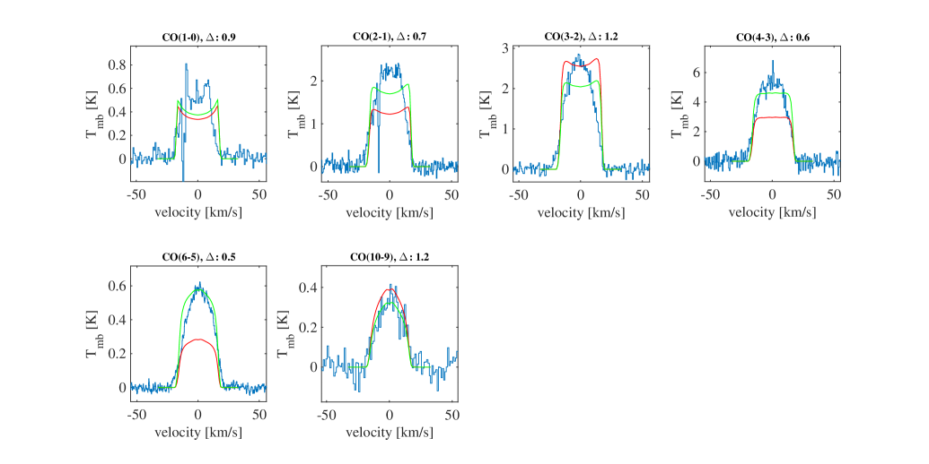
Figure 9: Best-fit CO models for TX Cam.The blue histograms are the observations. The red lines are the model lines, the green lines are the model lines scaled to the same integrated intensities as the observations. The velocities are given with respect to the $\varv_{\rm{LSR}}$ = 12.0 km s^-1.

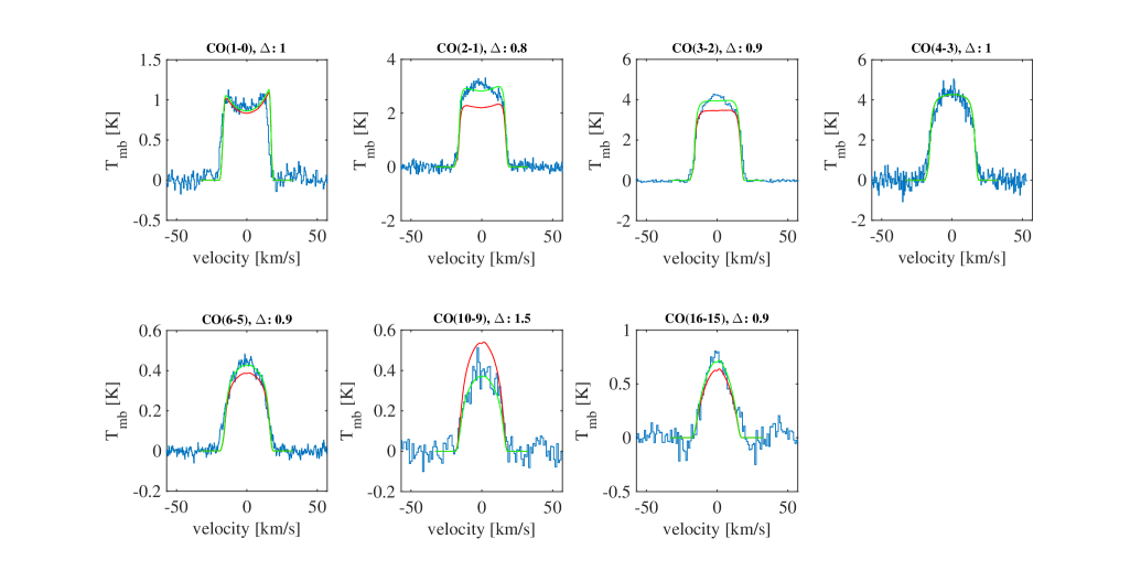
Figure 10: Best-fit CO models for IK Tau.The blue histograms are the observations. The red lines are the model lines, the green lines are the model lines scaled to the same integrated intensities as the observations. The velocities are given with respect to the $\varv_{\rm{LSR}}$ = 34.0 km s^-1.

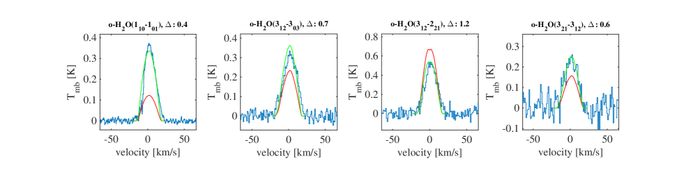
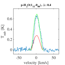
Figure 12: Best-fit o-H₂O and p-H₂O models of the HIFI Lines for TX Cam. The blue histograms are the observations. The red lines are the model lines, the green lines are the model lines scaled to the same integrated intensities as the observations. The velocities are given with respect to the $\varv_{\rm{LSR}}$ = 12.0 km s^-1.

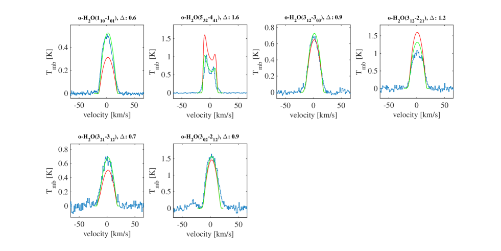
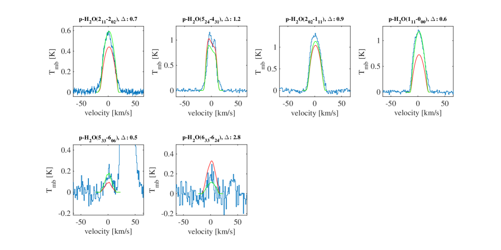
Figure 13: Best-fit o-H₂O and p-H₂O models of the HIFI Lines for IK Tau. The blue histograms are the observations. The red lines are the model lines, the green lines are the model lines scaled to the same integrated intensities as the observations. The velocities are given with respect to the $\varv_{\rm{LSR}}$ = 34.0 km s^-1.