Diffractive Propagation on Conic Manifolds
Séminaire Laurent Schwartz
January 26, 2016

Abstract.

In this survey, we review some applications and extensions of the author’s results with Richard Melrose on propagation of singularities for solutions to the wave equation on manifolds with conical singularities. These results mainly concern: the local decay of energy on noncompact manifolds with diffractive trapped orbits (joint work with Dean Baskin); singularities of the wave trace created by diffractive closed geodesics (joint work with G. Austin Ford); and the distribution of scattering resonances associated to such closed geodesics (joint work with Luc Hillairet).

1. Introduction

Consider the wave equation on a Riemannian manifold $X:$

$$\Box u=0\text{ on }\mathbb{R}\times X$$

where $\Box=D_{t}^{2}-\Delta_{g},$

$$\Delta_{g}=\sum\frac{1}{\sqrt{g}}D_{j}g^{jk}\sqrt{g}D_{k}$$

and $D_{j}\equiv i^{-1}{\partial}_{x_{j}}$.

If $X$ happens to be an odd dimensional Euclidean space, then Huygens’ Principle applies, i.e., the solution

$$\cos t\sqrt{\Delta}\delta_{q}$$

which has initial data a delta-function (and initial derivative zero) is supported exactly on sphere of radius ${\left\lvert{t}\right\rvert}.$ In even space dimensions, or on a general odd dimensional manifold, this principle is well known to fail, but quite a nice proxy for it persists: we in general have

$$\operatorname{sing-supp}u(t)\subset\big{\{}p:\ \text{there exists a geodesic of length }{\left\lvert{t}\right\rvert}\text{ with endpoints }p,q\big{\}}.$$

(Recall that the singular support of a distribution is the set of points near which is it not locally a smooth function.) A more precise result yet is the refinement of this statement to deal with the wavefront set of the distribution $u;$ $\operatorname{WF}u$ is a conic closed subset of $T^{*}X$ such that $\pi\operatorname{WF}u=\operatorname{sing-supp}u.$ Hörmander’s rather general theorem [Hormander9] on propagation of singularities tells us in this special case that for a solution $u$ of the wave equation, $\operatorname{WF}u$ is invariant under the (forward and backward) geodesic flow on $T^{*}X.$ Thus the initial wavefront given by (the lift to the light cone of) $N^{*}\{q\}$ then spreads into the conormal bundle of expanding distance spheres.

Generalizing this result to manifolds with boundary (with Dirichlet or Neumann boundary conditions) turns out be a rather complicated story. Chazarain [Ch:73] showed that singularities striking the boundary transversely simply reflect according to the usual law of geometric optics (conservation of energy and tangential momentum, hence “angle of incidence equals angle of reflection”) for the reflection of bicharacteristics. The difficulties arise, however, in the treatment of geodesics tangent to the boundary: in [Melrose-Sjostrand1] and [Melrose-Sjostrand2] Melrose–Sjöstrand showed that, at these “glancing points,” singularities may only propagate along certain generalized bicharacteristics. By parametrix constructions of Melrose [Melrose14] and Taylor [Taylor1], these $\mathcal{C}^{\infty}$ singularities do not propagate along concave boundaries (e.g. they do not “stick” to the exterior of a convex obstacle). Note that this last result ceases to be true in the analytic, rather than smooth, category.

A simple summary of some of the fundamental results in the subject is provided by Figure 1.

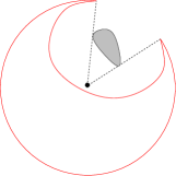
Figure 1. Singularities of the fundamental solution of the wave equation exterior to a convex obstacle.

This figure shows the singularities of the fundamental solution the wave equation in the exterior of a convex obstacle in the plane. There is (part of) a circular front of directly propagated singularities as well as a curved front of singularities reflected off the obstacle in accordance with Snell’s law. Most crucially, there are no singularities behind the obstacle in the “shadow region,” as a consequence of the parametrix construction of Melrose and Taylor.

By contrast, it has been known since the late 19th century (starting with work of Sommerfeld [Sommerfeld1]) that if the obstacle has a sharp corner, singularities do propagate, i.e., diffract, into the shadow region behind the obstacle. Figure 2 shows the fundemental solution of the wave equation in the exterior of a wedge; we can easily see a circular wave of singularities emanating from the tip of the wedge and giving rise to singularities in the shadow region.

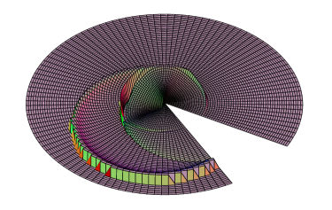
Figure 2. Singularities of the fundamental solution of the wave equation exterior to a wedge.

As alluded to above, general boundaries present special difficulties of their own, so in order to study the diffraction phenomenon in a simple setting, we now mostly set aside this class of manifolds, and focus on manifolds with conic singularities where wave equation solutions will exhibit diffraction, but the geometry of geodesics is relatively manageable.

2. Conic geometry

We define a conic manifold to be a manifold $X$ (of dimension $n$) with boundary $Y={\partial}X,$ and a Riemannian metric on $X^{\circ}$ such that in terms of some boundary defining function $x$ we have in a collar neighborhood of $Y,$

$$g=dx^{2}+x^{2}h$$

where $h$ is a smooth symmetric 2-cotensor such that $h|_{Y}$ is a metric on $Y.$ Note in particular that $g$ degenerates at ${\partial}X$ so as not to be a metric uniformly up to the boundary.

The upshot is that while $X$ looks like a manifold with boundary from the point of view of $\mathcal{C}^{\infty}$ structure, it is metrically a manifold with conic singularities: from the point of view of metric geometry, if we write the connected components of the boundary as

$$Y=\bigsqcup Y_{i}$$

then each boundary component $Y_{i}$ should be viewed as a cone point. (See Figure 3.)

Figure 3. Smooth structure, and Riemannian picture of $X$

The conic manifold as defined here should thus be viewed as a manifold with conic singularities already equipped with the blow-up that has desingularized it to a smooth manifold with boundary. Here the cost of having a smooth manifold is of course having a degenerate metric.

A very special case of a conic manifold is that of a surface obtained by gluing together two copies of the interior (or exterior) of a polygonal planar domain along their common edges. This gives a flat surface with cone points where the polygon had vertices. The study of the wave equation on the original domains with Dirichlet/Neumann conditions is equivalent to the study of odd/even solutions of the wave equation on the doubled manifold—see Hillairet [Hillairet:2005].

The behavior of geodesics on conic manifolds is of considerable interest near the cone point. The crucial observation is that it is in fact quite hard to aim a geodesic so as to hit the cone point: most will pass nearby and miss. Indeed, starting out near the cone point, there is a unique direction to aim in, in order to reach a nearby cone point.

Proposition 1 (Melrose–Wunsch [Melrose-Wunsch1]).

Every $y\in Y={\partial}X$ is the endpoint of a unique geodesic; these geodesics foliate a collar neighborhood of $Y$:

This is equivalent to a normal-form statement for the metric: we can find coordinates so that $h=h(x,y,dy)$ has no $dx$ components, and thus the curves $x=x_{0}\pm t,y=y_{0}$ are unit-speed geodesics.

A crucial point in trying to make sense of propagation of singularites is to make a reasonable definition of the continuation of a geodesic that reaches a cone point. There are two reasonable candidates for this definition, one more restrictive than the other, and both play a role here:

Definition 2.

We define geodesics passing through $\bigsqcup Y_{j}\equiv{\partial}X$ as follows:

• A diffractive geodesic is a geodesic which, upon reaching the boundary component $Y_{i}$ along a geodesic ending at a point $y\in Y_{i},$ immediately then leaves the boundary from some point $y^{\prime}\in Y_{i}.$

• A geometric geodesic is a geodesic which, upon reaching the boundary component $Y_{i}$ along a geodesic ending at a point $y\in Y_{i},$ immediately then leaves the boundary from some point $y^{\prime}\in Y_{i}$ such that $y,y^{\prime}$ are endpoints of a geodesic in $Y_{i}$ (w.r.t. the metric $h|_{Y_{i}})$ of length $\pi.$

• A strictly diffractive geodesic is one which is diffractive but not geometric.

A more intuitive definition of geometric geodesics is as follows: they are the geodesics that are locally approximable by families of geodesics in $X^{\circ}$. We refer the reader to [Melrose-Wunsch1] for more detail on these definitions.

3. Propagation of singularities on conic manifolds

Consider now solutions to the wave equation on a manifold with conic singularities. We always employ the Friedrichs extension of the Laplacian acting on $\mathcal{C}_{c}^{\infty}(X^{\circ}).$ (This stipulation is important only in dimension two, where $\Delta$ is not essentially self-adjoint.)

We now can (roughly) state the following:

Theorem 3 (Melrose–Wunsch [Melrose-Wunsch1]).

Singularities for solutions to the wave equation propagate along diffractive geodesics; strictly diffractive geodesics generically propagate weaker singularities than geometric geodesics.

The genericity condition is that the incident singularities not be precisely focused on the cone tip and applies, e.g., to Cauchy data that are conormal with respect to a manifold that is at most simply tangent to the hypersurfaces at constant distance from a cone tip. In this case—and in particular for the fundamental solution—we find that the diffracted wave for the fundamental solution is $(n-1)/2-\epsilon$ derivatives smoother than the main wavefront, where $n$ is the dimension of $X.$

We remark that this result has been subsequently generalized to cover the cases of manifolds with incomplete edge singularities [MVW1], as well as manifolds with corners [Va:04], [MeVaWu:13].

The rest of this paper is essentially applications and extensions of this result in various contexts.

4. Local energy decay on conic manifolds with Euclidean ends

Consider now a noncompact $n$-manifold $X$ with ends that are Euclidean. We will consider solutions to the wave equation

$$\Box u=0$$

on $X$ with compactly supported Cauchy data in the energy space.

If $X$ is a smooth manifold, it has long been known that the decay of local energy can be obstructed by the trapping of geodesics; recall that a geodesic is said to be forward- or backward-trapped if it remains in a compact set as $t\to\pm\infty.$ Classic work of Lax–Philips [Lax-Phillips1] and Morawetz [Morawetz:Decay] shows that, for odd $n,$ absence of trapping implies exponential local energy decay; on the other hand, results starting with Ralston [Ralston:Localized] show that trapping of rays implies that exponential local energy decay cannot hold. The usual line of reasoning in obtaining such estimates involves obtained bounds on the cutoff resolvent

$$\chi(\Delta-\lambda^{2})^{-1}\chi,\quad\chi\in\mathcal{C}_{c}^{\infty}.$$

It is well known that in odd dimensions this operator can be meromorphically continued from $\operatorname{Im}\lambda>0$ to $\mathbb{C},$ and its poles are known as resonances. Exponential local energy decay is then obtained by showing that no resonances lie in some strip $\operatorname{Im}\lambda>-\nu,$ $\nu>0$ (and that the resolvent has an upper bound with polynomial growth in this strip).

The situation with conic manifolds is thus interesting for the following reason: as soon as we have more than one cone point (or, indeed, at least one cone point if the manifold is non-simply connected) there must be trapped diffractive geodesics: we can simply continue traversing geodesics connecting the various cone points. An example of particular interest is (the double of) a domain exterior to one or more polygons in $\mathbb{R}^{2}$: diffractive geodesics can move along edges of one polygon and also along lines connecting vertices of two different polygons.

To what degree, one wonders, does this obstruct energy decay? The following theorem (which answers affirmatively a conjecture of Chandler-Wilde–Graham–Langdon–Spence [CWGLS:2012] for polygonal exterior domains) shows that the obstruction is very minor:

Theorem 4 (Baskin–Wunsch [BaWu:13]).

Assume that no three cone points in $X$ are collinear and no two are conjugate. Assume that geodesics missing the cone points escape to infinity at a uniform rate.

For $\chi\in\mathcal{C}_{c}^{\infty}(X),$ there exists $\delta>0$ such that the cut-off resolvent

$$\chi(\Delta-\lambda^{2})^{-1}\chi$$

can be analytically continued from $\operatorname{Im}\lambda>0$ to the region

$$\operatorname{Im}\lambda>-\rho\log{\lvert{\operatorname{Re}\lambda}\rvert},\ {\lvert{Re\lambda}\rvert}>\rho^{-1}$$

and for some $C,T>0$ enjoys the estimate

$${\left\lVert{\chi(\Delta-\lambda^{2})^{-1}\chi}\right\rVert}_{L^{2}\to L^{2}}\leq C{\lvert{\lambda}\rvert}^{-1}e^{T{\lvert{\operatorname{Im}\lambda}\rvert}}$$

in this region.

We contrast this with the the standard result for smooth non-trapping perturbations of Euclidean space. In that case the methods of Vainberg [Vainberg:Asymptotic] and Lax–Phillips [Lax-Phillips1] yield precisely the same resolvent estimate on $\mathbb{R}$ and a slightly stronger result on resonance-free regions: any region of the form $\operatorname{Im}\lambda>-\rho{\lvert{\log\operatorname{Re}\lambda}\rvert}$ is free of resonances outside a large disc. Thus the effect of diffractive trapping by cone points is extremely weak. Previous results in this direction include energy decay results of [Cheeger-Taylor2], Section 6, in certain special cases of conic singularities; analogous results for multiple inverse square potentials were previously proved by Duyckaerts [Duyckaerts1]. Burq [Burq:Coin] gave a precise description of the resonances in the closely related case of two convex analytic domains in the plane, one of which has a corner facing the other. The diffractive trajectory here bounces back and forth between the corner and the other obstacle, and Burq showed the associated resonances lie along a family of logarithmic curves.

We now briefly describe some results on evolution equations that follow from Theorem 4. We let $\mathcal{D}_{s}$ denote the domain of $\Delta^{s/2}$ (hence locally just $H^{s}$ away from cone points) and let $\sin t\sqrt{\Delta}/\sqrt{\Delta}$ be the wave propagator. Let $\chi$ equal $1$ on the set where $X$ is not isometric to $\mathbb{R}^{n}.$ In odd dimensions, the resolvent is a meromorphic function of $\lambda\in\mathbb{C}$ (with no difficulties at $\lambda=0$) so in this case Theorem 4 shows that there are only finitely many resonances in any horizontal strip in $\mathbb{C}.$ This enables us to show the following by a contour deformation argument:

Corollary 5.

Let $n$ be odd. Under the assumptions of Theorem 4, for all $A>0,$ small ${\epsilon}>0,$ $t>0$ sufficiently large, and $f\in\mathcal{D}_{1},$

$$\chi\frac{\sin t\sqrt{\Delta}}{\sqrt{\Delta}}\chi f=\sum_{\begin{subarray}{c}\lambda_{j}\in\operatorname{Res}(\Delta)\\ \operatorname{Im}\lambda>-A\end{subarray}}\sum_{m=0}^{M_{j}}e^{-it\lambda_{j}}t^{m}w_{j,m}+E_{A}(t)f$$

where the sum is of resonances of $\Delta,$ i.e. over the poles of the meromorphic continuation of the resolvent, and the $w_{j,m}$ are the associated resonant states corresponding to $\lambda_{j}.$ The error satisfies

$${\left\lVert{E_{A}(t)}\right\rVert}_{\mathcal{D}_{1}\to L^{2}}\leq C_{\epsilon}e^{-(A-{\epsilon})t}.$$

In particular, since the resonances have imaginary part bounded above by a negative constant, $\chi\frac{\sin t\sqrt{\Delta}}{\sqrt{\Delta}}\chi f$ is exponentially decaying in this case.

Another corollary is a local smoothing estimate for the Schrödinger equation. As it comes from the resolvent estimate on $\mathbb{R},$ this is again lossless as compared to the situation on free $\mathbb{R}^{n}$:

Corollary 6.

Suppose $u$ satisfies the Schrödinger equation on $X$:

$$i^{-1}{\partial}_{t}u(t,z)+\Delta u(t,z) =0$$

$$u(0,z) =u_{0}(z)\in L^{2}(X)$$

Under the assumptions of Theorem 4, for all $\chi\in C^{\infty}_{c}(X)$, $u$ satisfies the local smoothing estimate without loss:

$$\int_{0}^{T}{\left\lVert{\chi u(t)}\right\rVert}_{\mathcal{D}_{1/2}}^{2}\,dt\leq C_{T}{\left\lVert{u_{0}}\right\rVert}_{L^{2}}^{2}.$$

The elements of the proof of Theorem 4 are twofold. The first step is to show that a very weak Huygens principle holds. We recall that in nontrapping manifolds, a solution to the wave equation with compactly supported initial data is eventually smooth—this is the usual “weak Huygens principle.” Here we show instead that the solution eventually gets as smooth as we like:

Proposition 7.

Let $\chi\in\mathcal{C}_{c}^{\infty}(X).$ For any $s\in\mathbb{R},$ there exists $T_{s}\gg 0$ such that whenever $t>T_{s},$

$$\chi U(t)\chi:H^{r}\to H^{r+s}$$

for all $r.$

The second part of the theorem is a modification of the celebrated parametrix construction of Vainberg [Vainberg:Asymptotic] (see also [Tang-Zworski1]). This argument in its original form builds a parametrix for the resolvent out of the fundamental solution to the wave equation, assuming that the latter satisfies the weak Huygens principle; the new variant, by contrast, makes the weaker assumption of the output of Proposition 7 and produces a very slightly weaker result (smaller resonance-free region).

Among the further applications of this line of reasoning is the following theorem on Strichartz estimates for exterior polygonal domains (joint work with Baskin and Marzuola) [BaskinMarzuolaWunsch:2014]): for an exterior polygonal domain where the only trapped geodesics are strictly diffractive (and where no three vertices are collinear) we find that the same Strichartz estimates for the Schrödinger equation hold as on Euclidean space (locally in time for Neumann conditions, and globally for Dirichlet).

5. The wave trace

If $X$ is a compact Riemannian manifold without boundary let

$$(\phi_{j},\lambda_{j}^{2})$$

denote the eigenfunctions and eigenvalues of $\Delta.$ One might like to study the “inverse spectral problem” of using the $\lambda_{j}$ to characterize $X$ by forming a useful generating function out of the $\lambda_{j}.$ An obvious but not directly useful one might be

$$\sum_{j}\delta(\lambda-\lambda_{j}),$$

but a much more tractable one is the Fourier transform of this quantity,

$$\sum_{j}e^{-it\lambda_{j}}.$$

The utility of this generating function stems from its identification as

$$\operatorname{Tr}U(t),$$

where

$$U(t)\equiv e^{-it\sqrt{\Delta}}$$

is the “half-wave” evolution operator, mapping functions on $X$ to (certain) solutions to the wave equation. If we can say something about the trace of $U(t)$ in terms of the geometry of $X,$ we can thus hope to learn something about spectral geometry.

In the setting of smooth boundaryless manifolds, we have the following classical results on the wave trace. Let

$$\operatorname{L-Spec}(X)=\{0\}\bigcup\big{\{}\pm\text{lengths of periodic geodesics on }X\big{\}}.$$

Theorem 8 (Chazarain [Chazarain1], Duistermaat–Guillemin [Duistermaat-Guillemin1]; cf. also Colin de Verdière [Co:73a], [Co:73b]).

$$\operatorname{sing-supp}\operatorname{Tr}U(t)\subset\operatorname{L-Spec}(X).$$

This allows one to dream of “hearing” lengths of closed geodesics, but does not rule out the possibility that the allowable singularities do not, in fact, arise. The presence of honest singularities is, however, guaranteed by:

Theorem 9 (Duistermaat–Guillemin [Duistermaat-Guillemin1]).

Let $L$ be the length of an nondegenerate periodic closed geodesic $\gamma$ on $L$ that is isolated in the length spectrum. Then near $t=L$ we have

$$\operatorname{Tr}U(t)\sim\frac{L_{0}}{2\pi}i^{\sigma}{\left\lvert{I-P}\right\rvert}^{-1/2}(t-L)^{-1},$$

where

• $L_{0}$ is the length of the primitive closed geodesic if $\gamma$ is an iterate of a shorter one.

• $\sigma$ is the Morse index of the variational problem for a periodic geodesic, evaluated at $\gamma.$

• $P$ is the linearized Poincaré map, obtained as the linearization at $\gamma$ of the first return map to a hypersurface of the phase space, transverse to $\gamma.$

Note that the nondegeneracy condition in the hypotheses is simply the condition that $I-P$ be nonsingular.

The generalization of Theorem 8 to compact conic manifolds is straightforward: let

$$\operatorname{Diff-L-Spec}(X)=\{0\}\bigcup\big{\{}\pm\text{lengths of periodic diffractive geodesics on }X\big{\}}.$$

Theorem 10 (Wunsch [Wunsch2]).

On a conic manifold $X,$

$$\operatorname{sing-supp}\operatorname{Tr}U(t)\subset\operatorname{Diff-L-Spec}{X}.$$

The singularities at lengths of geodesics in $X^{\circ}$ are easily seen to be described by the same formula given by Duistermaat–Guillemin, but the geodesics interacting through conic points are not so simple. We consider $\gamma$ a closed, strictly diffractive geodesic undergoing $k$ diffractions and traversing geodesic segments $\gamma_{1},\dots,\gamma_{k}$ connecting cone points $Y_{i_{1}},\dots Y_{i_{k}}.$ Recall that the hypothesis that the geodesic be strictly diffractive means that it interacts with each cone point by entering and leaving on a pair of geodesics that cannot be uniformly locally approximated by geodesics in $X^{\circ}.$ This is generically the case for all closed geodesics. Assume further that the length $L$ of $\gamma$ is isolated in the length spectrum, and make the additional nondegeneracy hypothesis that no two cone points along the geodesic are conjugate to one another. Note that the following was previously known by work of Hillairet [Hillairet:2005] in the important special case of flat surfaces with conic singularities (hence in particular for doubles of polygons).

Theorem 11 (Ford–Wunsch [1411.6913]).

Near $t=L,$

$$\operatorname{Tr}U(t)\sim\int e^{i(t-L)\xi}a(\xi)\,d\xi$$

where

(1) $$a(\xi)\sim L_{0}\cdot(2\pi)^{\frac{kn}{2}}\,e^{\frac{ik(n-3)\pi}{4}}\,\chi(\xi)\,\xi^{-\frac{k(n-1)}{2}}\prod_{j=1}^{k}i^{-m_{\gamma_{j}}}\,\mathcal{D}_{j}\,\mathcal{W}_{j}\ \text{as $|\xi|\to\infty$}.$$

Here, $\chi\in\mathcal{C}^{\infty}(\mathbb{R})$ is $1$ for $\xi>1$ and $0$ for $\xi<0.$ Note that the power of $\xi$ is such that we obtain greater smoothness as the number of diffractions increases. The leading order singularity as a function of $t$ is proportional to $(t-L+i0)^{-1+k(n-1)/2}$ (but is multiplied by $\log(t-L+i0)$ if the power is an integer).

As before $L_{0}$ denotes the length of the “primitive” geodesic if $\gamma$ is an iterate of a shorter one. The integers $m_{\gamma_{j}}$ are simply the Morse indices of the variational problems associated to traveling from one cone point to the next, evaluated at $\gamma_{j}.$

We will now explain the factors $\mathcal{D}_{j}$ and $\mathcal{W}_{j}.$

The terms $\mathcal{D}_{j}$ are associated to the diffractions through each successive cone point $Y_{i_{j}}.$ They are constructed as follows. Each cone point $Y_{i_{j}}$ is equipped with a metric $h_{i_{j}}\equiv h\rvert_{Y_{i_{j}}}.$ It thus has a Laplace-Beltrami operator $\Delta_{i_{j}}$ and we may use the functional calculus to take functions of this operator. In particular, let

$$\nu_{i_{j}}\equiv\sqrt{\Delta_{Y_{i_{j}}}+\left(\frac{2-n}{2}\right)^{2}}.$$

We then form the operator family

$$e^{-it\nu_{i_{j}}}:L^{2}(Y_{i_{j}})\to L^{2}(Y_{i_{j}}).$$

This is essentially a “half Klein Gordon propagator” on the link of the cone point (i.e., a boundary component). Now let $\kappa(\bullet)$ denote the Schwartz kernel of an operator. Supposing that the diffractive geodesic $\gamma$ enters $Y_{i_{j}}$ at the point $y$ and leaves from point $y^{\prime},$ we set

$$\mathcal{D}_{j}\equiv\kappa(e^{-i\pi\nu_{i_{j}}})[y,y^{\prime}].$$

The propagator kernel is of course not continuous in general, however note that the strictly diffractive nature of the geodesic ensures that $y$ and $y^{\prime}$ are not connected by a geodesic of length $\pi$ in the link, which in turn precisely ensures, by propagation of singularities, that the Schwartz kernel of the time-$\pi$ Klein Gordon propagator is smooth near $(y,y^{\prime}),$ hence the evaluation of this distribution makes sense.

Now we turn to $\mathcal{W}_{j}$. These quantities are associated to the geodesic segments $\gamma_{j}$ connecting successive cone points. They are best described in terms of Jacobi fields, but can also be viewed as a proxy for a quantity involving the derivative of the expenential map, hence a substitute for the term involving the Poincaré map in the Duistermaat–Guillemin formula. Note that the exponential map from one cone point to the next does not make sense, since any small perturbation of the geodesic $\gamma_{j}$ will miss the next cone point entirely rather than simply hitting it at a different point. Correspondingly, if we let $\mathbf{J}$ be a set of Jacobi fields that are orthonormal to $\gamma_{j}$ and at $\gamma_{j}(0)$ give an orthonormal basis of $TY_{i_{j}}$ then $\mathbf{J}$ becomes singular as we approach the end of $\gamma_{j}$ at $Y_{i_{j+1}}.$ On the other hand, the metric is also singular at cone points, in the sense that it vanishes on $TY,$ so we can nonetheless make sense of the determinant

$$\operatorname{det}_{g}\mathbf{J}\rvert_{Y_{i_{j+1}}}.$$

Then we have

$$\mathcal{W}_{j}\equiv\big{\lvert}\operatorname{det}_{g}\mathbf{J}\rvert_{Y_{i_{j+1}}}\big{\rvert}^{-1/2}.$$

This quantity can be made to look more like the derivative of an exponential map as follows: we set

(2) $$\Theta_{j}=(\operatorname{length}(\gamma_{j})^{-(n-1)})\big{\lvert}\operatorname{det}_{g}\mathbf{J}\rvert_{Y_{i_{j+1}}}\big{\rvert}.$$

Consider the case in which $Y_{j}$ is a “fictitious” cone point obtained by blowing up a smooth point $p_{0}$ on a manifold. Then Jacobi vector fields tangent to $Y_{j}$ are obtained as lifts under the blow-down map of Jacobi fields vanishing at $p_{0},$ and $\Theta_{j}$ becomes a standard expression for $\operatorname{det}D\exp_{Y_{j}}(\bullet)$ in terms of Jacobi fields, at least when evaluated in $X^{\circ}$ (cf. [Be:77]): in that case we simply have

$$\Theta_{j}=\operatorname{det}_{g}\big{\lvert}D\exp_{Y_{j}}(\bullet)\big{\rvert}.$$

Since $\mathcal{W}_{j}=\operatorname{length}(\gamma_{j})^{-(n-1)/2}\Theta_{j}^{-1/2}$ we recover the relationship with the exponential map in the case of a trivial cone point.

In rough outline, the proof of Theorem 11 goes as follows. We know explicitly what the wave propagator look like on a model product cone $\mathbb{R}_{+}\times Y_{j}$ endowed with the scale invariant metric $dx^{2}+x^{2}h_{0}(y,dy)$—this is a computation of Cheeger–Taylor [Cheeger-Taylor1], [Cheeger-Taylor2] involving bravura use of the Hankel transform. In particular, we can evaluate the symbol of the diffracted wavefront explicitly in that case. More generally, in [Melrose-Wunsch1] the author and Melrose prove that near a cone point, the diffracted front of the wave propagator is guaranteed to be a conormal distribution. The first new step is therefore to show that in the non-product case, the principal symbol of the diffracted front is still, modulo adjustments involving comparing half-densities on the two spaces, given by the same expression as in the product case where we use the model metric $dx^{2}+x^{2}h\rvert_{x=0}(y,dy).$ This involves comparing the two propagators and showing that the difference between model and exact propagators can be estimated by a Morawetz inequality near the cone tip.

Having understood the effect of a single diffraction, we then proceed as follows. We take a microlocal partition of unity $A_{j}$ on $X,$ where for technical reasons the $A_{j}$ are restricted to be simply cutoff functions near each boundary component $Y_{i}$ but are otherwise fully localized in phase space. We then decompose the wave trace as follows: fix small times $t_{j}$ with $\sum t_{j}=T.$ Then by cyclicity of the trace

$$\operatorname{Tr}U(t)=\sum_{i_{0},\dots,i_{N}}\operatorname{Tr}\sqrt{A_{i_{0}}}U(t-T)A_{i_{1}}U(t_{1})A_{i_{2}}\dots A_{t_{N}}U(t_{N})\sqrt{A_{i_{0}}}.$$

By propagation of singularities, this term is guaranteed to be trivial unless there is a diffractive geodesic successively passing through the microsupports of the $A_{i_{j}}$’s, hence we may throw away most of this sum. The remaining terms are then computed by a stationary phase computation, gluing together the propagators for “free” propagation through $X^{\circ}$ with those for the diffractive interaction with cone points (this was the same strategy previously used by Hillairet in [Hillairet:2005] as well as by the author in [Wunsch2]).

6. Lower bounds for resonances

While $\operatorname{Tr}U(t)$ only makes sense (even distributionally) on a compact manifold, if we return to the setting of Section 4 where we have a noncompact manifold with Euclidean ends, we may still make sense of an appropriately renormalized wave trace, and use the diffractive trace formula (Theorem 11) to obtain lower bounds on resonances.

In odd dimensions, we let $\mathcal{A}$ denote the generator of the wave group, and hence $e^{t\mathcal{A}}$ the wave group itself; likewise we let $\mathcal{A}_{0}$ be the generator of the wave group on Euclidean space. We then have the trace formula

(3) $$\operatorname{Tr}(e^{t\mathcal{A}}-e^{t\mathcal{A}_{0}})=\sum_{\lambda_{j}\in\operatorname{Res}}e^{-i\lambda_{j}t},\ t>0$$

where the sum is over the resonances, counted with multiplicity (see e.g. [Sjostrand-Zworski5] for the details of how to makes sense of this difference of operators in a wide variety of contexts). This result in various settings was first proved by Bardos-Guillot-Ralston [Bardos-Guillot-Ralston1], Melrose [MR83j:35128], and Sjöstrand-Zworski [Sjostrand-Zworski5]; an analogous result in even dimensions can be found in [Zw:99].

Now if we can actually guarantee the existence of singularities in the (renormalized) wave trace, a Tauberian theorem of Sjöstrand-Zworski [Sjostrand-Zworski3] allows us to deduce from (3) in a lower bound on the number of resonances in logarithmic regions in $\mathbb{C}.$ Fortunately, Theorem 11 applies equally well in this context, and we obtain a lower bound on the number of resonances as follows. Let

$$N_{\rho}(r)=\#\{\text{Resonances in }{\lvert{\lambda}\rvert}<r,\ \operatorname{Im}\lambda\geq-\rho\log{\lvert{\operatorname{Re}{\lambda}}\rvert}\}.$$

Then we have:

Theorem 12 (Hillairet–Wunsch).

Under the geometric assumptions of Theorem 4, let $L$ be the length of a closed, strictly diffractive geodesic $\gamma$ undergoing $k$ diffractions. Assume, in the notation of Theorem 11, that all the diffraction coefficients $\mathcal{D}_{j}$ are nonzero along $\gamma;$ assume also that there are no closed diffractive geodesics beside iterates of this one having length in $L\mathbb{N}.$ Then for all ${\epsilon}>0,$

$$N_{\rho}(\rho)\geq C_{\rho,\epsilon}r^{1-\epsilon}$$

provided

$$\rho>\frac{(n-1)k}{2L}$$

A detailed proof, which simply consists of using the trace formula (Theorem 11) in (3) together with the Tauberian theorem of [Sjostrand-Zworski3], can be found in [Ga:15]. Note that the bound on $\rho$ written here is that which we obtain by considering the whole sequence of singularities of the wave trace obtained by considering arbitrary iterates of the geodesic $\gamma.$ We remark that the distinction between the trace of the full wave group and $\operatorname{Tr}U(t)$ is immaterial for this purpose since the former is twice the real part of the latter, and it is not difficult to verify from examination of (1) that the singularities arising from iterates of a given geodesic cannot all be purely imaginary.

The optimal $\rho$ here is generally obtained by choosing $\gamma$ to be the geodesic that traverses the longest geodesic segment connecting a pair of distinct cone points, back and forth (assuming the diffraction coefficients are nonvanishing). If $D_{\text{max}}$ denotes the greatest distance between a pair of cone points, then we have a closed geodesic of length $2D_{\text{max}}$ with $k=2,$ and we obtain the bound

$$\rho>\frac{(n-1)}{2D_{\text{max}}}.$$

Remarkably, this theorem is essentially sharp, as was shown by Galkowski, who has produced an effective version of the Vainberg argument previously employed in [BaWu:13]:

Theorem 13 (Galkowski [Ga:15]).

Let $D_{\text{max}}$ be the greatest distance between two cone points. For any $\epsilon>0$ the constant $\rho$ in Theorem 4 can be taken to be $(n-1)/(2D_{\text{max}})-\epsilon,$ i.e. $N_{\rho}(r)$ is bounded for all $\rho<(n-1)/2D_{\text{max}}.$

Since $N_{\rho}$ is bounded for $\rho<(n-1)/2D_{\text{max}}$ and (subject to the nondegeneracy hypotheses of Theorem 12) almost linearly growing for $\rho>(n-1)/2D_{\text{max}},$ we find that in any set near the critical curve $\operatorname{Im}\lambda=-((n-1)/2D_{\text{max}})\log{\lvert{\operatorname{Re}\lambda}\rvert}$ of the form

$$\big{(}-\frac{n-1}{2D_{\text{max}}}-{\epsilon}\big{)}\log{\lvert{\operatorname{Re}\lambda}\rvert}<\operatorname{Im}\lambda<\big{(}-\frac{n-1}{2D_{\text{max}}}+{\epsilon}\big{)}\log{\lvert{\operatorname{Re}\lambda}\rvert},\quad{\left\lvert{\lambda}\right\rvert}>{\epsilon}^{-1}$$

there are infinitely many resonances. The intuition behind the importance of the longest geodesic connecting two cone points is that repeatedly traversing this segment back and forth is the way in which a trapped singularity can diffract least frequently. Since each diffraction loses considerable energy owing to the smoothing effect of diffraction, a resonant state propagating back and forth along this geodesic is the one that loses energy to infinity at the slowest rate.