IceCube and GRB neutrinos propagating in quantum spacetime

Abstract

Two recent publications have reported intriguing analyses, tentatively suggesting that some aspects of IceCube data might be manifestations of quantum-gravity-modified laws of propagation for neutrinos. We here propose a strategy of data analysis which has the advantage of being applicable to several alternative possibilities for the laws of propagation of neutrinos in a quantum spacetime. In all scenarios here of interest one should find a correlation between the energy of an observed neutrino and the difference between the time of observation of that neutrino and the trigger time of a GRB. We select accordingly some GRB-neutrino candidates among IceCube events, and our data analysis finds a rather strong such correlation. This sort of studies naturally lends itself to the introduction of a “false alarm probability”, which for our analysis we estimate conservatively to be of 1$\%$. We therefore argue that our findings should motivate a vigorous program of investigation following the strategy here advocated.

I INTRODUCTION

The prediction of a neutrino emission associated with gamma ray bursts (GRBs) is generic within the most widely accepted astrophysical models fireball . After a few years of operation IceCube still reports icecubeUPDATEgrbnu no conclusive detection of GRB neutrinos, contradicting some influential predictions waxbig ; meszabig ; dafnebig ; otherbig of the GRB-neutrino observation rate by IceCube. Of course, it may well be the case that the efficiency of neutrino production at GRBs is much lower than had been previously estimated small1 ; small2 ; small3 . However, from the viewpoint of quantum-gravity/quantum-spacetime research it is interesting to speculate that the IceCube results for GRB neutrinos might be misleading because of the assumption that GRB neutrinos should be detected in very close temporal coincidence with the associated $\gamma$-rays: a sizeable mismatch between GRB-neutrino detection time and trigger time for the GRB is expected in several much-studied models of neutrino propagation in a quantum spacetime (see Refs.gacLRR ; jacobpiran ; gacsmolin ; grbgac ; gampul ; urrutia ; gacmaj ; myePRL ; gacGuettaPiran ; steckerliberati and references therein).

This possibility was preliminarily explored in Ref.gacGuettaPiran using only IceCube data from April 2008 to May 2010, and focusing on 3 weak but intriguing candidate GRB neutrinos (see Ref.icecubeCERN ; icecubetesi ): a 1.3 TeV neutrino 1.95^o off GRB090417B with detection time 2249 seconds before the trigger of GRB090417B, a 3.3 TeV neutrino 6.11^o off GRB090219 and detection time 3594 seconds before the GRB090219 trigger, and a 109 TeV neutrino 0.2^o off GRB091230A and detection time some 14 hours before the GRB091230A trigger. The analysis reported in Ref.gacGuettaPiran would have been more intriguing if the 109 TeV event could be viewed as a promising cosmological-neutrino candidate, but for that event there was a IceTop-tank trigger coincidence. A single IceTop-tank trigger is not enough to firmly conclude that the event was part of a cosmic-ray air shower, but of course that casts a shadow on the interpretation of the 109-TeV event as a GRB neutrino.

Unaware of the observations reported in Ref.gacGuettaPiran , recently Stecker et al. reported in Ref.steckerliberati an observation which also might encourage speculations about neutrino propagation in quantum spacetime. Ref.steckerliberati noticed that IceCube data are presently consistent with a $\sim 2PeV$ cutoff for the cosmological-neutrino spectrum, and that this could be due to novel processes (like “neutrino splitting”steckerliberati ; gacLRR ) that become kinematically allowed in the same class of quantum-spacetime models considered in Ref.gacGuettaPiran .

The study we are here reporting was motivated by these previous observations of Refs.gacGuettaPiran and steckerliberati . Like Ref.gacGuettaPiran our focus is on the hypothesis of GRB neutrinos with quantum-spacetime properties, also exploiting the fact that, while Ref.gacGuettaPiran was limited to IceCube data up to May 2010, the amount of data now available from IceCube IceCube is significantly larger. Conceptually the main issue we wanted to face is indeed related to the amount of IceCube data: as studies like these start to contemplate larger and larger groups of “GRB-neutrino candidates” some suitable techniques of statistical analysis must be adopted, and (unlike Refs.gacGuettaPiran and steckerliberati ) we wanted to devise a strategy of analysis applicable not only to one “preferred model”, but to a rather wide class of scenarios for the properties of the laws of propagation of neutrinos in a quantum spacetime.

As discussed more quantitatively below, the effects on propagation due to spacetime quantization can be systematic or of “fuzzy” type. Combinations of systematic effects and fuzziness are also possible, and this is the hypothesis most challenging from the viewpoint of data analysis. We came to notice that in all these scenarios one should anyway find a correlation between the energy of the observed GRB neutrino and the difference between the time of observation of that neutrino and the trigger time of the relevant GRB. Intriguingly our data analysis finds a rather strong such correlation, and we therefore argue that our findings should motivate a vigorous program of investigation following the strategy here advocated.

II Quantum-spacetime-propagation models and strategy of analysis

The class of scenarios we intend to contemplate finds motivation in some much-studied models of spacetime quantization (see, e.g., jacobpiran ; gacsmolin ; gacLRR ; grbgac ; gampul ; urrutia ; gacmaj ; myePRL and references therein) and, for the type of data analyses we are interested in, has the implication that the time needed for a ultrarelativistic particle to travel from a given source to a given detector receives a quantum-spacetime correction, here denoted with $\Delta t$. We focus on the class of scenarios whose predictions for energy ($E$) dependence of $\Delta t$ can all be described in terms of the formula (working in units with the speed-of-light scale “$c$” set to 1)

$$\Delta t=\eta_{X}\frac{E}{M_{P}}D(z)\pm\delta_{X}\frac{E}{M_{P}}D(z)\,.$$ (1)

Here the redshift- ($z$-)dependent $D(z)$ carries the information on the distance between source and detector, and it factors in the interplay between quantum-spacetime effects and the curvature of spacetime. As usually done in the relevant literature jacobpiran ; gacsmolin ; gacLRR we take for $D(z)$ the following form:

$$D(z)=\int_{0}^{z}d\zeta\frac{(1+\zeta)}{H_{0}\sqrt{\Omega_{\Lambda}+(1+\zeta)^{3}\Omega_{m}}}\,,$$ (2)

where $\Omega_{\Lambda}$, $H_{0}$ and $\Omega_{0}$ denote, as usual, respectively the cosmological constant, the Hubble parameter and the matter fraction, for which we take the values given in Ref.PlanckCosmPar . With $M_{P}$ we denote the Planck scale ($\simeq 1.2\,\cdotp 10^{28}eV$) while the values of the parameters $\eta_{X}$ and $\delta_{X}$ in (1) characterize the specific scenario one intends to study. In particular, in (1) we used the notation “$\pm\delta_{X}$” to reflect the fact that $\delta_{X}$ parametrizes the size of quantum-uncertainty (fuzziness) effects. Instead the parameter $\eta_{X}$ characterizes systematic effects: for example in our conventions for positive $\eta_{X}$ and $\delta_{X}=0$ a high-energy neutrino is detected systematically after a low-energy neutrino (if the two neutrinos are emitted simultaneously).

The dimensionless parameters $\eta_{X}$ and $\delta_{X}$ can take different values for different particles gacLRR ; myePRL ; mattiLRR ; szabo1 , and it is of particular interest for our study that in particular for neutrinos some arguments have led to the expectation of an helicity dependence of the effects (see, e.g., Refs.gacLRR ; mattiLRR and references therein). Therefore even when focusing only on neutrinos one should contemplate four parameters, $\eta_{+}$, $\delta_{+}$, $\eta_{-}$, $\delta_{-}$ (with the indices $+$ and $-$ referring of course to the helicity). The parameters $\eta_{X},\delta_{X}$ are to be determined experimentally. When non-vanishing, they are expected to take values somewhere in a neighborhood of 1, but values as large as $10^{3}$ are plausible if the solution to the quantum-gravity problem is somehow connected with the unification of non-gravitational forces gacLRR ; wilczek ; hsuHIGGSES while values smaller than 1 find support in some renormalization-group arguments (see, e.g., Ref.hsuHIGGSES2 ).

Presently for photons the limits on $\eta_{\gamma}$ and $\delta_{\gamma}$ are at the level of $|\eta_{\gamma}|\lesssim 1$ and $\delta_{\gamma}\lesssim 1$ fermiNATURE ; gacNATUREPHYSICS2015 , but for neutrinos we are still several orders of magnitude below 1 steckerliberati ; gacLRR . This is mainly due to the fact that the observation of cosmological neutrinos is rather recent, still without any firm identification of a source of cosmological neutrinos, and therefore the limits are obtained from terrestrial experiments (where the distances travelled are of course much smaller than the ones relevant in astrophysics).

For reasons that shall soon be clear we find convenient to introduce a “distance-rescaled time delay” $\Delta t^{*}$ defined as

$$\Delta t^{*}\equiv\Delta t\frac{D(1)}{D(z)}$$ (3)

so that (1) can be rewritten as

$$\Delta t^{*}=\eta_{X}\frac{E}{M_{P}}D(1)\pm\delta_{X}\frac{E}{M_{P}}D(1)\,.$$ (4)

This reformulation of (1) allows to describe the relevant quantum-spacetime effects, which in general depend both on redshift and energy, as effects that depend exclusively on energy, through the simple expedient of focusing on the relationship between $\Delta t$ and energy when the redshift has a certain chosen value, which in particular we chose to be $z=1$. If one measures a certain $\Delta t$ for a candidate GRB neutrino and the redshift $z$ of the relevant GRB is well known, then one gets a firm determination of $\Delta t^{*}$ by simply rescaling the measured $\Delta t$ by the factor $D(1)/D(z)$. And even when the redshift of the relevant GRB is not known accurately one will be able to convert a measured $\Delta t$ into a determined $\Delta t^{*}$ with accuracy governed by how much one is able to still assume about the redshift of the relevant GRB. In particular, even just the information on whether a GRB is long or short can be converted into at least a very rough estimate of redshift.

Of course a crucial role is played in analyses such as ours by the criteria for selecting GRB-neutrino candidates. We need a temporal window (how large can the $\Delta t$ be in order for us to consider a IceCube event as a potential GRB-neutrino candidate) and we need criteria of directional selection (how well the directions estimated for the IceCube event and for the GRB should agree in order for us to consider that IceCube event as a potential GRB-neutrino candidate). While our analysis shall not include the above-mentioned 109-TeV neutrino (from Ref.gacGuettaPiran ), we do use it to inspire a choice of the temporal window: assuming a 109-TeV GRB neutrino could be detected within 14 hours of the relevant GRB trigger time, an analysis involving neutrinos with energies up to 500 TeV should allow for a temporal window of about 3 days, and an analysis involving neutrinos with energies up to, say, 1000 TeV should allow for a temporal window of about 6 days. Considering the rate of GRB observations of about 1 per day, we opt for focusing on neutrinos with energies between 60 TeV and 500 TeV, allowing for a temporal window of 3 days. Widening the range of energies up to, say, 1000 TeV would impose us indeed a temporal window of about 6 days, rendering even more severe one of the key challenges for this sort of analysis, which is the one of multiple GRB candidates for a single IceCube event. As directional criteria for the selection of GRB-neutrino candidates we consider the signal direction PDF depending on the space angle difference between GRB and neutrino: $P(\nu,GRB)=(2\pi\sigma^{2})^{-1}\exp(-\frac{|\vec{x}_{\nu}-\vec{x}_{GRB}|^{2}}{2\sigma^{2}})$, a two dimensional circular Gaussian whose standard deviation is $\sigma=\sqrt{\sigma_{GRB}^{2}+\sigma_{\nu}^{2}}$, asking the pair composed by the neutrino and the GRB to be at angular distance compatible within a 2$\sigma$ region.

A key observation for our analysis is that whenever $\eta_{+}$, $\eta_{-}$, $\delta_{+}$, $\delta_{-}$ do not vanish one should expect on the basis of (4) a correlation between the $|\Delta t^{*}|$ and the energy of the candidate GRB neutrinos. The interested reader will immediately see that this is obvious when $\delta_{+}=\delta_{-}=0$. It takes only a little bit more thinking to notice that such a correlation should be present also when $\delta_{+}\neq 0$ and/or $\delta_{-}\neq 0$ with $\eta_{+}=\eta_{-}=0$, as a result of how the fuzzy effects have range that grows with the energy of the GRB neutrinos. We provide support for this conclusion in Fig.1.

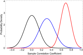
Figure 1: Here we illustrate the different expectations one should have for the correlation on which we focus, assuming all neutrinos are just background neutrinos (black), assuming $10\%$ of neutrinos are background while $90\%$ are GRB neutrinos with $\eta_{+}=\eta_{-}=0$, $\delta_{+}=\delta_{-}=5$ (blue), or assuming $10\%$ of neutrinos are background while $90\%$ are GRB neutrinos with $\eta_{+}=\eta_{-}=15$, $\delta_{+}=\delta_{-}=5$ (red). The probability densities were computed assuming that the spectrum of the neutrinos decreases quadratically with energy ($E^{-2}$) between 60 and 500 TeV, that the neutrinos would be observed only if within a 3-day window of the relevant GRB, and, for simplicity, that all relevant GRBs are exactly at redshift of 1. This probability densities were obtained for the hypothetical case of 50 candidate GRB neutrinos. The figure shows that 50 candidate GRB neutrinos would be enough for the most likely correlation outcome in the scenario with $\eta_{+}=\eta_{-}=0$, $\delta_{+}=\delta_{-}=5$ to be a rather unlikely outcome for the “pure-background hypothesis.” Actually, much less than 50 candidate GRB neutrinos would be enough for the most likely correlation outcome in the scenario with $\eta_{+}=\eta_{-}=15$, $\delta_{+}=\delta_{-}=5$ to be a very unlikely outcome for the pure-background hypothesis.

 

III RESULTS

Our data set is for four years of operation of IceCube IceCube , from June 2010 to May 2014. Since the determination of the energy of the neutrino plays such a crucial role in our analysis we include only IceCube “shower events” (for “track events” the reconstruction of the neutrino energy is far more problematic and less reliable TRACKnogood1 ). We have 21 such events within our 60-500 TeV energy window, and we find that 9 of them fit the requirements introduced in the previous section for candidate GRB neutrinos. The properties of these 9 candidates that are most relevant for our analysis are summarized in Table 1 and Figure 2.

	​​​ E ​​​​ [TeV] ​​​	GRB	z	$\Delta t^{*}$ [s]
IC9	63.2	110503A	1.613	50227	*
IC19	71.5	111229A	1.3805	53512	*
IC42	76.3	131117A	4.042	5620
		131118A	1.497 *	-98694	*
		131119A	?	-146475
IC11	88.4	110531A	1.497 *	124338	*
IC12	104.1	110625B	1.497 *	108061	*
IC2	117.0	100604A	?	10372
		100605A	1.497 *	-75921	*
		100606A	?	-135456
IC40	157.3	130730A	1.497 *	-120641	*
IC26	210.0	120219A	1.497 *	153815	*
		120224B	?	-117619
IC33	384.7	121023A	0.6 *	-289371	*

Table 1: Among the 21 “shower neutrinos” with energy between 60 and 500 TeV observed by IceCube between June 2010 and May 2014 only 9 fit our directional and temporal criteria for GRB-neutrino candidates, and yet for 3 of them there is more than one GRB to be considered when pairing up neutrinos and GRBs. The last column highlights with an asterisk the 9 GRB-neutrino candidates ultimately selected by our additional criterion of maximal correlation. Also shown in table are the values of redshift attributed to the relevant GRBs: the redshift is known only for GRB111229A and GRB110503A (plus GRB131117A, which however ends up not being among the GRBs selected by the maximal-correlation criterion). GRB111229A and GRB110503A are long GRBs and we assume that the average of their redshifts (1.497) could be a reasonably good estimate of the redshifts of the other long GRBs relevant for our 9 GRB-neutrino candidates. These are the 6 estimated values of redshift $z=1.497^{*}$, the asterisk reminding that it is a “best guess” value. For analogous reasons we place an asterisk close to the value of 0.6 which is our best guess for the redshift of the only short GRB in our sample. The first column lists the “names” given by IceCube to the neutrinos that end up being relevant for our analysis. Also notice that 5 of our GRB-neutrino candidates are “late neutrinos” ($\Delta t^{*}>0$), while the other 4 are “early neutrinos” ($\Delta t^{*}<0$): this might be of interest to some readers but plays no role in our study since our correlations involve the absolute value of $\Delta t^{*}$.

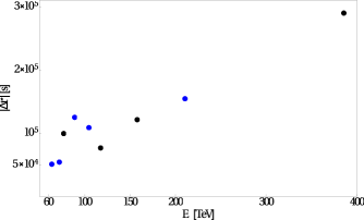
Figure 2: Points here in figure correspond to the 9 GRB-neutrino candidates highlighted with an asterisk in the last column of Table 1. Blue points correspond to “late neutrinos” ($\Delta t^{*}>0$), while black points correspond to “early neutrinos” ($\Delta t^{*}<0$).

In commenting Table 1 we start by noticing that for some IceCube events our selection criteria produce multiple GRB-neutrino candidates (and the situation would have been much worse if we had considered a wider energy range and a correspondingly wider temporal window). Since we have two cases with 3 possible GRB partners and one case with a pair of possible GRB partners, we must contemplate 18 alternative descriptions of our 9 GRB-neutrino candidates. As neutrino telescopes gradually accrue more and more such events the number of combinations to be considered in analyses such as ours will grow very large. We propose that in general this issue of multiple candidates should be handled, consistently with the nature of the hypothesis being tested, by focusing on the case that provides the highest correlation. This might appear to introduce a bias toward higher values of the correlation, but, as we shall soon argue, the significance of such an analysis is not given by the correlation itself but rather requires the evaluation of a “false alarm probability”, and for the false alarm probability this criterion for handling multiple candidates introduces no bias (see below).

Another issue reflected by Table 1 comes from the fact that for only 3 of the GRBs involved in this analysis the redshift is known. We must handle only one short GRB of unknown redshift, and we assume for it a redshift of 0.6, which is a rather reasonable rough estimate for a short GRB (but we shall contemplate also values of 0.5 and of 0.7). For some of our long GRBs we do have a redshift determination and we believe that consistently with the hypothesis here being tested one should use those known values of redshift for obtaining at least a rough estimate of the redshift of long GRBs for which the redshift is unknown. This is illustrated by the 9 GRB-neutrino candidates marked by an asterisk in table 1: those 9 candidates include 8 long GRBs, 2 of which have known redshift, and we assign to the other 6 long GRBs the average ${\bar{z}}$ of those two values of redshift (${\bar{z}}=1.497$). As it will be reported in the PhD thesis of Ref.Juniorthesis , we have checked that our results do not depend strongly on the what is assumed about unknown redshifts, be it assuming that these redshifts follow the distribution of GRBs observed in photons or simply assuming different values of ${\bar{z}}$. We shall document a bit of this insight here below, by providing our results both assuming this criterion of the ${\bar{z}}$ and assuming simply a redshift of 2 for all long GRBs of unknown redshift. We feel that estimating a ${\bar{z}}$ from the “data points” is the only reasonable way to proceed, since we do not expect that the redshift distribution of GRBs observed also in neutrinos should look much like the redshift distribution of GRBs observed only in photons. However we imagine that some readers might have been more comfortable if we assumed for our long GRBs of unknown redshift the average value of redshift of GRBs observed in photons, which is indeed of about 2.

Having specified these further prescriptions, we can proceed to compute the correlation between $|\Delta t^{*}|$ and energy for our 9 GRB-neutrino candidates. Because of the fact that for some of our neutrinos there is more than one possible GRB partner we end up having 18 such values of correlation, and remarkably they are all very high: the highest of these 18 values is of 0.951 (the corresponding 9 neutrino-GRB pairs are highlighted by an asterisk in Table 1 and are shown in Figure 2), and even the lowest of these 18 values of correlation is still of 0.802. In Table 2 we show how the evaluation of the maximum correlation for our 9 GRB-neutrino candidates would change upon replacing our ${\bar{z}}$ with a redshift of $2$, for long GRBs, and upon replacing the value of 0.6 we assumed for the redshift of the short GRB in our collection with 0.5 or 0.7.

	$z_{long}=\bar{z}$	$z_{long}=2$
${z_{short}}=0.5$	0.958	0.953
${z_{short}}=0.6$	0.951	0.960
${z_{short}}=0.7$	0.941	0.964

Table 2: Adopting our “$\bar{z}$ criterion” for long GRBs whose redshift is not known and z=0.6 for short GRBs one gets as maximal correlation for our data the impressive value of 0.951. Here we show how this estimate changes if one assigns to short GRBs the alternative values of redshift of 0.5 and 0.7 and/or one replaces our $\bar{z}$ with a redshift of 2.

The class of quantum-spacetime scenarios we are considering predicts a non-vanishing (and possibly large) correlation, and we did find on data very high values of correlation. This in itself however does not quantify what is evidently the most interesting quantity here of interest, which must be some sort of “false alarm probability”: how likely it would be to have accidentally data with such good agreement with the expectations of the quantum-spacetime models here contemplated? We need to estimate how often a sample composed exclusively of background neutrinos would produce accidentally 9 or more GRB-neutrino candidates with correlation comparable to (or greater than) those we found in data. We do this by performing $10^{5}$ randomizations of the times of detection of the 21 IceCube neutrinos relevant for our analysis, keeping their energies fixed, and for each of these time randomizations we redo the analysis just as if they were real data. Our observable is a time-energy correlation and by randomizing the times we get a robust estimate of how easy (or how hard) it is for a sample composed exclusively of background neutrinos to produce accidentally a certain correlation result. In the analysis of these fictitious data obtained by randomizing the detection times of the neutrinos we handle cases with neutrinos for which there is more than one possible GRB partner by maximizing the correlation, in the sense already discussed above for the true data. We ask how often this time-randomization procedure produces 9 or more GRB-neutrino candidates with correlation $\geq 0.951$, and remarkably we find that this happens only in 0.03$\%$ of cases.

In Table 3 we report a preliminary investigation of how this result of a 0.03$\%$ false alarm probability depends on the assumptions we made for redshifts. Table 3 is in the same spirit of what was reported in our Table 2 for the estimates of the correlation. Each entry in Table 2 recalculates the false alarm probability just like we did above to obtain the result of 0.03$\%$, but now considering some alternative possibilities for the assignment of redshifts to GRBs whose redshift is actually unknown. Once again for long GRBs we consider two possibilities, the ${\bar{z}}$ discussed above and redshift of $2$, while for short GRBs we consider values of redshift of 0.5, 0.6 and 0.7. Table 3 shows that our false alarm probability does not change much within this range of exploration of the redshift assignments.

	$z_{long}=\bar{z}$	$z_{long}=2$
${z_{short}}=0.5$	0.03 %	0.04 %
${z_{short}}=0.6$	0.03 %	0.02 %
${z_{short}}=0.7$	0.04 %	0.01 %

Table 3: Adopting our “$\bar{z}$ criterion” for long GRBs whose redshift is not known and z=0.6 for short GRBs one gets a false alarm probability of 0.03$\%$. Here we show how this estimate changes if one assigns to short GRBs the alternative values of redshift of 0.5 and 0.7 and/or one replaces our $\bar{z}$ with a redshift of 2.

Our next objective is to see how things change if one is “unreasonably conservative” in assessing the implications of our prescription for handling cases where there is more than one possible GRB partner for a neutrino. We are proposing that one should address this multi-candidate issue in the way that maximizes the correlation, and this evidently introduces some bias toward higher values of the correlation. However, as already stressed above, when we randomize (fictitious) detection times we handle the multi-candidate issue in exactly the same way, by maximizing the correlation, so that overall there is no bias for the false alarm probability. It is nonetheless interesting to notice that one still obtains a rather low false alarm probability even when comparing the minimum correlation for our true data to the maximum correlation for the fictitious data obtained by randomizing neutrino detection times. So we now ask how often the fictitious data obtained by randomizing neutrino detection times produce 9 or more GRB-neutrino candidates with correlation $\geq 0.803$ ($0.803$ being, as noticed above, the lowest possible value of correlation for our true data), but for the fictitious data we still handle cases with neutrinos having more than one possible GRB partner by maximizing the correlation. Even this procedure, which is evidently biased toward lower values of the false alarm probability, only gives a false alarm probability of $\simeq 1\%$. Table 4 explores the dependence on assumptions for redshift of the value of $0.803$ for the lowest correlation obtainable from the true data, while Table 5 explores analogously the dependence on assumptions for redshift of our result for the “unreasonably conservative estimate of the false alarm probability.”

	$z_{long}=\bar{z}$	$z_{long}=2$
${z_{short}}=0.5$	0.844	0.869
${z_{short}}=0.6$	0.803	0.849
${z_{short}}=0.7$	0.751	0.822

Table 4: Adopting our “$\bar{z}$ criterion” for long GRBs whose redshift is not known and z=0.6 for short GRBs one gets as minimal correlation for our data a still high value of 0.803. Here we show how this estimate changes if one assigns to short GRBs the alternative values of redshift of 0.5 and 0.7 and/or one replaces our $\bar{z}$ with a redshift of 2.

	$z_{long}=\bar{z}$	$z_{long}=2$
${z_{short}}=0.5$	0.7 %	0.6 %
${z_{short}}=0.6$	1.0 %	0.6 %
${z_{short}}=0.7$	1.5 %	0.8 %

Table 5: Adopting our “$\bar{z}$ criterion” for long GRBs whose redshift is not known and z=0.6 for short GRBs we obtain an “unreasonably conservative estimate of the false alarm probability” which is still only 1.0$\%$. Here we show how this estimate changes if one assigns to short GRBs the alternative values of redshift of 0.5 and 0.7 and/or one replaces our $\bar{z}$ with a redshift of 2.

IV Toward estimating model parameters

In searching for evidence of quantum-spacetime effects on neutrino propagation our approach has the advantage of allowing to study at once a variety of scenarios, the scenarios obtainable by all sorts of combinations of values for $\eta_{+}$, $\eta_{-}$, $\delta_{+}$, $\delta_{-}$. This is due to the fact that positive correlation between $\Delta t^{*}$ and $E$ is expected whenever one or more of the parameters $\eta_{+}$, $\eta_{-}$, $\delta_{+}$, $\delta_{-}$ are non-zero. Our approach performs very well in comparing the hypothesis “all the GRB-neutrino candidates actually are background neutrinos” to the hypothesis “some of the GRB-neutrino candidates truly are GRB neutrinos governed by Eq.(1) with one or more of the parameters $\eta_{+}$, $\eta_{-}$, $\delta_{+}$, $\delta_{-}$ having non-zero value.” It does so in ways that are rather robust with respect to the assumptions made about the redshift of the relevant GRBs and with respect to the presence of some background neutrinos among the GRB-neutrino candidates.

Our false-alarm probabilities are still not small enough to worry about that, but if it happens that the experimental situation develops positively for our scenario then one will of course be interested in estimating model parameters, i.e. comparing how well different choices of values of the parameters of the model match the available data. This is clearly harder within our approach. In particular it surely requires some reasonable estimate of the amount of background neutrinos present among the GRB-neutrino candidates. Testing the hypothesis that all the GRB-neutrino candidates actually are background neutrinos is evidently simpler than testing the hypothesis that some of the GRB-neutrino candidates are background and some other are truly GRB neutrinos: for the latter one would need to specify how many are background and how many are GRB neutrinos.

While we postpone contemplating these issues until (and if) the experimental situation evolves accordingly, we still find appropriate to offer here at least a rudimentary attempt of interpretation of the data on the basis of the parameters of our reference Eq.(1), assuming naively that all our GRB-neutrino candidates actually are GRB neutrinos. Because of the accordingly explorative nature of the observations reported in this section, we shall be satisfied taking as reference the 9 GRB-neutrino candidates marked with an asterisk in Table 1 and considered in Fig.2, i.e. the maximum-correlation 9-plet. If the experimental situation develops in such a way to provide motivation for more refined estimations of model parameters, the relevant procedures should not only rely on some estimate of the amount of background neutrinos but should also handle the fact that some neutrinos have more than one possible GRB partner, in the same spirit we adopted for the estimates of the false-alarm probability given in the previous section. At the present stage we find sufficient not only to neglect background neutrinos and consider exclusively the maximum-correlation 9-plet, but also to focus on a simplified version of the phenomenological model. As first simplification we assume $\eta_{+}+\eta_{-}=0$, which is reasonably consistent with the fact that in Fig.2 one sees about an equal number of candidate “early neutrinos” and candidate “late neutrinos”. In addition we further restrict our attention to the case $\delta_{+}=\delta_{-}$, so that we must only be concerned with the parameters $\eta_{+}$ and $\delta_{+}$ (with then $\eta_{-}=-\eta_{+}$, $\delta_{-}=\delta_{+}$).

Having specified these restrictions we first take a very simple-minded approach and assume that the features shown in Fig.2 are all due to Eq.(1). This in particular means we are naively assuming that there are no background neutrinos, that the estimates of GRB redshifts given in table 1 are exact, and that points in Fig.2 fail to be on a straight line exclusively because of the effects of the parameter $\delta_{+}$ (and $\delta_{-}$, with $\delta_{-}=\delta_{+}$). This leads to $|\eta_{+}|=22\pm 2$ and $\delta_{+}=6\pm 2$.

Next we perform a Bayesian analysis to derive posterior distributions of unknown parameters. We assume again simple-mindedly that there are no background neutrinos, and we handle as unknown parameters not only the parameters of our model, $|\eta_{+}|$ and $\delta_{+}$, but also the standard deviation $\delta z$ of the normal distribution that we tentatively assume to describe the redshift distribution of long GRBs observed also in neutrinos. As mean value of this normal distribution we take 1.497, following the argument discussed in the previous section. For the redshift distribution of short GRBs observed also in neutrinos (which is relevant for only one of our GRB-neutrino candidates) we simply assume a normal distribution with mean value 0.6 and standard deviation of 0.2. In order to evaluate the marginalized posterior probability density functions of the parameters $|\eta_{+}|$, $\delta_{+}$ and $\delta z$ we use the Markov chain Monte Carlo technique, with uniform priors with ranges $0\leq\eta\leq 50$, $0\leq\delta\leq 10$ and $0\leq\delta z\leq 1$. Uncertainties for the energies of the neutrinos (see Ref. IceCube ) were also taken into account. This Bayesian analysis determines $\delta z$ to be $\delta z=0.45\pm 0.17$, and for the parameters of our model gives $|\eta_{+}|=23\pm 2$, $\delta_{+}=4.7\pm 1.5$, which is consistent with what we had concluded in the previous paragraph ($|\eta_{+}|=22\pm 2$, $\delta_{+}=6\pm 2$) on the basis of more simple-minded considerations.

V OUTLOOK

As mentioned, our work took off from the analogous study reported in Ref.gacGuettaPiran , with additional motivation found in what had been reported in Ref.steckerliberati . We looked within IceCube data from June 2010 to May 2014 for the same feature which had been already noticed in Ref.gacGuettaPiran , in an analysis based on much poorer IceCube data for the period from April 2008 to May 2010. The study of Ref.gacGuettaPiran was intriguing but ultimately appeared to be little more than an exercise in data-analysis strategy, since it could only consider 3 neutrinos, none of which could be viewed as a promising GRB-neutrino candidate. The 109-TeV event considered in Ref.gacGuettaPiran could be easily dismissed as likely the result of a cosmic-ray air shower, and the other two neutrinos were of much lower energy, energies at which atmospheric neutrinos are very frequent. Yet what we found here is remarkably consistent with what had been found in Ref.gacGuettaPiran . Particularly the 109-TeV event would be a perfect match for the content of our Figure 2, as the interested reader can easily verify. We chose to rely exclusively on data unavailable to Ref.gacGuettaPiran , IceCube data from June 2010 to May 2014, and on these new data alone the feature is present very strongly, characterized by a false alarm probability which we estimated fairly at $0.03\%$ and ultraconservatively at $1\%$. We feel this should suffice to motivate a vigorous program of further investigation of the scenarios here analyzed.

Particularly over these last few decades of fundamental physics, results even more encouraging than ours have then gradually faded away, as more data was accrued, and we are therefore well prepared to see our neutrinos have that fate. We are more confident that our strategy of analysis will withstand the test of time. The main ingredient of novelty is the central role played by the correlation between the energy of a neutrino and the difference between the time of observation of that neutrino and the trigger time of a GRB. The advantage of focusing on this correlation is that it is expected in a rather broad class of phenomenological models of particle propagation in a quantum spacetime, which was here summarized in our Eq.(1). Moreover, by analyzing a few representative cases of simulated data we find Juniorthesis that such correlation studies are rather robust with respect to uncertainties in the estimates of the rates of background neutrinos, and this could be valuable: extrapolating to higher energies known facts about the rate of atmospheric neutrinos is already a challenge, but for analyses such as ours one would also need to know which percentage of cosmological neutrinos are due to GRBs, an estimate which at present is simply impossible to do reliably. Comparing for example our approach to the strategy of analysis adopted in Ref.gacGuettaPiran one can see immediately that the strategy of analysis adopted in Ref.gacGuettaPiran is inapplicable when $\delta_{X}\neq 0$ (whether or not $\eta_{X}=0$). When $\eta_{X}\neq 0$, $\delta_{X}=0$ we find Juniorthesis that our approach and the approach of Ref.gacGuettaPiran perform comparably well if the rate of background neutrinos is well known, but ours is indeed more robust with respect to uncertainties in the estimates of the rates of background neutrinos.

References

- (1) T. Piran, Phys. Rep. 333, 529 (2000).
- (2) IceCube Collaboration: M. G. Aartsen et alia, ApJ 805 L5 (2015); M. G. Aartsen et alia, arXiv:1601.06484v1.
- (3) E. Waxman and J.N.Bahcall, Phys. Rev. Lett. 78, 2292 (1997).
- (4) J.P. Rachen and P. Meszaros, [in C.A. Meegan, R.D. Preece, and T.M. Koshut (ed.), American Institute of Physics Conference Series 428, 776 (1998)]
- (5) D. Guetta, D. Hooper, J. Alvarez-Miniz, F. Halzen and E. Reuveni, Astroparticle Physics 20, 429 (2004).
- (6) M. Ahlers, M.C. Gonzalez-Garcia and F. Halzen, Astroparticle Physics 35, 87 (2011).
- (7) P. Baerwald, S. Hummer and W. Winter, Phys. Rev. D 83, 067303 (2011).
- (8) S. Hummer, P. Baerwald and W. Winter, Phys. Rev. Lett. 108, 231101 (2012).
- (9) B. Zhang and P. Kumar, arXiv:1210.0647
- (10) G. Amelino-Camelia, Living Rev. Rel. 16, 5 (2013).
- (11) U. Jacob and T. Piran, Nature Phys. 3, 87 (2007).
- (12) G. Amelino-Camelia and L. Smolin, Phys.Rev. D 80, 084017 (2009).
- (13) G. Amelino-Camelia, J. Ellis, N.E. Mavromatos, D.V. Nanopoulos and S. Sarkar, Nature 393, 763 (1998).
- (14) R. Gambini and J. Pullin, Phys. Rev. D59, 124021 (1999).
- (15) J. Alfaro, H.A. Morales-Tecotl and L.F. Urrutia, Phys. Rev. Lett. 84, 2318 (2000).
- (16) G. Amelino-Camelia and S. Majid, Int. J. Mod. Phys. A 15, 4301 (2000).
- (17) R.C. Myers and M. Pospelov, Phys. Rev. Lett. 90, 211601 (2003).
- (18) G. Amelino-Camelia, D. Guetta and T. Piran, APJ 806 Number 2, 269 (2015).
- (19) F. W. Stecker, S. T. Scully, S. Liberati and D. Mattingly, Phys. Rev. D 91, 045009 (2015).
- (20) CERN Courier, 31 May 2012, IceCube observations challenge ideas on cosmic-ray origins (http://cerncourier.com/cws/article/cern/49675)
- (21) N. Whitehorne, A search for high-energy neutrino emission from Gamma-ray Bursts, Ph.D. thesis (https://docushare.icecube.wisc.edu/dsweb/Get/Document-60879/thesis.pdf); see in particular figures 6.1 and 6.2 and their captions.
- (22) IceCube Collaboration: M. G. Aartsen et al, Phys. Rev. Lett. 111, 021103 (2013); Science 342, 1242856 (2013); Phys. Rev. Lett. 113, 101101 (2014); Proceedings of Science 1081 (ICRC2015).
- (23) G. Rosati, G. Amelino-Camelia, A. Marciano and M. Matassa, Phys. Rev. D 92, 124042 (2015)
- (24) Planck Collaboration: P. A. R. Ade et alia, arXiv:1502.01589v2.
- (25) S. P. Robinson and F. Wilczek, Phys. Rev. Lett. 96 (2006) 231601
- (26) X. Calmet, S. D. H. Hsu and D. Reeb, Phys. Rev. Lett. 101 (2008) 171802
- (27) X. Calmet, S. D. H. Hsu and D. Reeb, Phys. Rev. D81 (2010) 035007
- (28) D. Mattingly, Living Rev.Rel. 8, 5 (2005).
- (29) R.J. Szabo, Phys.Rept. 378, 207 (2003).
- (30) A.A. Abdo et alia [Fermi LAT/GBM Collaborations], Nature 462, 331 (2009).
- (31) V. Vasileiou, J. Granot, T. Piran and G. Amelino-Camelia, Nature Physics 11, 344–346 (2015).
- (32) IceCube Collaboration: M. G. Aartsen et alia, Phys. Rev. Lett. 115, 081102.
- (33) IceCube Collaboration: M. G. Aartsen et alia, JINST 9, P03009 (2014); M. Kadler et alia, arXiv:1602.02012v2, to appear on Nature Physics; Joel Bressieux, Testing and comparison of muon energy estimators for the IceCube neutrino observatory, Master Thesis (http://lphe.epfl.ch/publications/diplomas/jb.master.pdf).
- (34) G. D’Amico, PhD thesis (in preparation).