Localized travelling waves in the asymptotic suction boundary layer

Abstract

We present two spanwise-localized travelling wave solutions in the asymptotic suction boundary layer, obtained by continuation of solutions of plane Couette flow. One of the solutions has the vortical structures located close to the wall, similar to spanwise-localized edge states previously found for this system. The vortical structures of the second solution are located in the free stream far above the laminar boundary layer and are supported by a secondary shear gradient that is created by a large-scale low-speed streak. The dynamically relevant eigenmodes of this solution are concentrated in the free stream, and the departure into turbulence from this solution evolves in the free stream towards the walls. For invariant solutions in free-stream turbulence, this solution thus shows that that the source of energy of the vortical structures can be a dynamical structure of the solution itself, instead of the laminar boundary layer.

1 Introduction

In the last few decades dynamical systems theory has been established as a new paradigm for studying turbulence. The foundation for this progress has been the computation of invariant solutions of the Navier-Stokes equations which capture crucial features of turbulent flows at moderate Reynolds numbers. Fully 3D and fully nonlinear invariant solutions, in the form of equilibria, travelling waves, and periodic orbits, have been computed for canonical confined shear flows such as pipe flow, plane Couette and plane Poiseuille flow (Kawahara et al., 2012). Such studies in minimal flow units have produced spatially periodic and thus infinitely extended invariant solutions. More recently, spatially localized solutions have been constructed for flows in large domains (Gibson & Brand, 2014; Brand & Gibson, 2014; Zammert & Eckhardt, 2014). These localized solutions are better suited to investigate transitional turbulence, which usually originates in localized turbulent patches and shows rich spatio-temporal dynamics.

A natural further step is to extend invariant solutions from confined flows to external flows and eventually free-stream turbulence. Similarities between external and internal flows near transition suggest that this extension is possible; for example, both plane Couette flow and the boundary layer exhibit roll-streak coherent structures (Nagata, 1990; Robinson, 1991) and localized turbulent spots that grow into the surrounding laminar flow. However, invariant solutions have not yet been computed for developing boundary layers. The key difficulty is that the growth of the boundary layer thickness with distance from the leading edge breaks the continuous translation symmetry of the flow in the downstream direction. This broken symmetry disallows downstream travelling wave solutions, which are the dynamically simplest possible invariant solutions and the most straightforward to compute.

We will therefore consider a modified, canonical, and well-studied open boundary layer, the asymptotic suction boundary layer (ASBL). In the ASBL, constant suction through a porous wall counteracts the growth of the boundary layer, and far from the leading edge a parallel streamwise invariant flow is established (Schlichting, 2004). Several invariant solutions have been computed for the ASBL. Edge-tracking methods in a minimal flow unit yield a periodic orbit of very long period (Kreilos et al., 2013). In a spanwise extended domain, a spanwise-localized relative periodic orbit has been found (Khapko et al., 2013, 2014). The only known travelling waves of the ASBL have been constructed by Deguchi & Hall (2014) (hereafter referred to as DH14). Like the periodic orbits of Kreilos et al. (2013), one of the DH14 travelling waves is dominated by vortical structures attached to the wall. The other has vortical structures at a large distance from the wall. DH14 thus terms these travelling waves “wall-mode” and “free-stream” coherent structures, respectively. Both of the DH14 ASBL travelling waves are localized in the wall-normal direction but periodic in the spanwise and streamwise directions. The applicability of the high-Reynolds number asymptotics within the framework of vortex-wave interactions (Hall & Smith, 1991) in growing boundary layers was investigated in two further papers by the same authors (Deguchi & Hall, 2015b, a).

In this paper, we demonstrate the existence of wall-mode and free-stream travelling-wave solutions of the ASBL that are localized in both the spanwise and the wall-normal directions. Like the DH14 solutions, the wall mode has tilted, counter-rotating vortices and high- and low-speed streaks that reside in the near-wall laminar shear region, while the vortices of the free-stream lie within the free stream and support streaks closer to the wall. We show that the free-stream travelling wave is dynamically detached from the wall and supports turbulence localized in both the spanwise and the wall-normal direction. While transitioning to turbulence, the localized turbulent region in the cross-flow plane slowly and almost isotropically invades laminar flow at constant front velocity until the wall is reached.

2 Methods

The ASBL consists of an incompressible fluid streaming over a flat plate into which it is homogeneously sucked at a constant rate. Far from the leading edge the suction exactly compensates the growth of the boundary layer and a translationally invariant laminar profile emerges (Schlichting, 2004). The laminar downstream velocity increases from zero at the wall to the free-stream velocity $U_{\infty}$, with a characteristic length scale $\delta=\nu/V_{S}$ determined by the kinematic viscosity $\nu$ and the suction velocity $V_{S}$. Denoting the downstream, wall-normal and spanwise directions as $x,y$ and $z$ respectively, and the corresponding components of velocity as $u,v,w$, the governing Navier-Stokes equations for $\mathbf{u}$ and pressure $p$ are

$$\partial_{t}\mathbf{u}+(\mathbf{u}\cdot\mathbf{\nabla})\mathbf{u}=-\mathbf{\nabla}p+\nu\mathbf{\nabla}^{2}\mathbf{u},$$ (1)

together with the incompressibility condition $\mathbf{\nabla}\cdot\mathbf{u}=0$ and the boundary conditions

$$\mathbf{u}(x,0,z)=(0,-V_{S},0),\qquad\mathbf{u}(x,y\rightarrow\infty,z)=(U_{\infty},-V_{S},0).$$ (2)

The laminar flow profile of the ASBL

$$\mathbf{u}_{L}(x,y,z)=(U_{\infty}(1-{\mathrm{e}}^{-y/\delta}),-V_{S},0)$$ (3)

is an analytic solution to this system of equations. The laminar $99\%$ boundary layer thickness, i.e. the value of $y$ at which $u(y)=0.99U_{\infty}$, is $\delta_{99\%}=4.605\delta$. The Reynolds number for the ASBL is defined as

$$\mbox{{Re}}=\frac{U_{\infty}\delta}{\nu}=\frac{U_{\infty}}{V_{S}}.$$ (4)

In numerical simulation we enforce the upper boundary condition at a finite height $y=H$, leading to a slight modification of the laminar profile,

$$\mathbf{u}_{0}(x,y,z)=(U^{*}(1-{\mathrm{e}}^{-y/\delta}),-V_{S},0),$$ (5)

with $U^{*}=U_{\infty}/(1-{\mathrm{e}}^{-H/\delta})$. This profile approaches $\mathbf{u}_{L}$ and the computational flow approaches the ASBL as $H\rightarrow\infty$. At $H=20\delta$ the value of $\delta_{99\%}$ differs by only $10^{-6}$ from its value at $H\rightarrow\infty$. Our simulations are performed with a parallel version of the pseudospectral code channelflow (Gibson, 2012), which simulates the Navier-Stokes equations for incompressible fluids in rectangular domains with two periodic directions and no-slip boundary conditions in the third direction. The spatial discretization uses Fourier modes in the streamwise and spanwise directions and Chebyshev polynomials in the wall-normal direction. Travelling wave solutions are found with a Newton-Krylov-hookstep algorithm (Viswanath, 2007, 2009), and predictor-corrector parameter continuation is performed by extrapolating three known solutions at different parameter values and correcting with Newton’s method afterwards.

To construct localized solutions of the ASBL, we perform a homotopy continuation from known solutions of plane Couette flow, the spanwise-localized equilibria EQ7-1 and EQ7-2 of Gibson & Brand (2014). Choosing a coordinate system in which the lower plate at $y=0$ is motionless and the upper plate at $y=H$ moves at speed $U_{\infty}$, a homotopy from plane Couette to ASBL conditions can be defined by increasing $V_{S}$ from $0$ to a finite value such that $H/\delta\gg 1$. Starting at plane Couette conditions with $U_{\infty}H/\nu=1600$ and $V_{S}=0$, we increase $V_{S}$, $H$ and $L_{x}$ and lower $\nu$ until we arrive at ABSL flow conditions with $\mbox{{Re}}=U_{\infty}/V_{S}\simeq 2000$ and $HV_{S}/\nu=H/\delta=20$. Then within the ASBL we vary the Reynolds number by increasing $\nu$ and $V_{S}$ proportionally so that $\delta=\nu/V_{S}$ remains constant. In what follows all lengths, velocities, and times are normalized by $\delta,U_{\infty},$ and $\delta/U_{\infty}$.

3 Results

3.1 Spanwise-localized wall-mode and free-stream coherent structures in the ASBL

We successfully continued both EQ7-1 and EQ7-2 to ASBL conditions with $[L_{x},H,L_{z}]$ at $[4\pi,20,24\pi]$ and $[5.5\pi,20,24\pi]$ respectively, and with a resolution of $[48,121,512]$ grid points. In the ASBL these states are spanwise-localized travelling waves similar to the free-stream and wall-mode travelling waves of DH14, respectively. We henceforth refer to them as the free-stream coherent structure (FCS) and the wall mode (WM) of the ASBL. After continuation into the ASBL the FCS retains EQ7-1’s shift-reflect symmetry

$$[u,v,w](x,y,z)=[u,v,-w](x+L_{x}/2,y,-z)$$ (6)

and the WM retains EQ7-2’s $z$-mirror symmetry

$$[u,v,w](x,y,z)=[u,v,-w](x,y,-z).$$ (7)

These symmetries were enforced throughout the continuations.

Figure 1 shows the bifurcation diagram of the FCS and WM states in the ASBL with Re as control parameter. The two states appear as lower branches in saddle-node bifurcations at $\mbox{{Re}}=968$ for FCS and $\mbox{{Re}}=348$ for WM. The structure of the velocity fields shows little variation with Re; i.e. the states do not change qualitatively along the continuation. We choose to discuss them somewhat above their respective bifurcation points, at $\mbox{{Re}}=1000$ and $\mbox{{Re}}=400$, respectively.

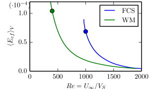
Figure 1: Bifurcation diagram of the free-stream (FCS) and wall-mode (WM) solutions showing volume-averaged cross-flow energy $\langle E_{cf}\rangle_{V}=\frac{1}{V}\int_{V}(v^{2}+w^{2})\mathrm{d}x\,\mathrm{d}y\,\mathrm{d}z$ as a function of Reynolds number. Both solutions emerge as lower branches in saddle-node bifurcations. The two circles indicate the states depicted in figure 2(c-f).

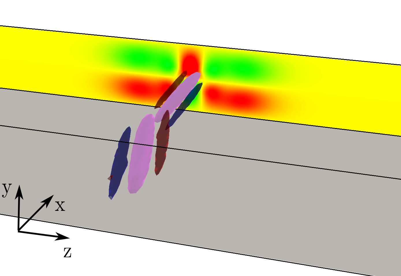
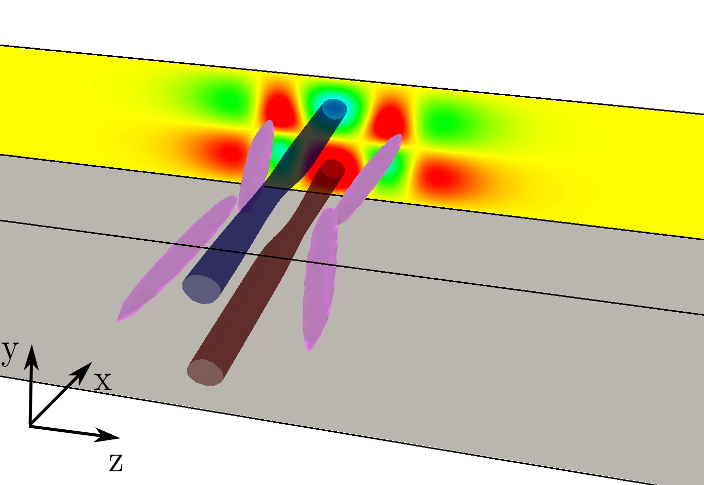
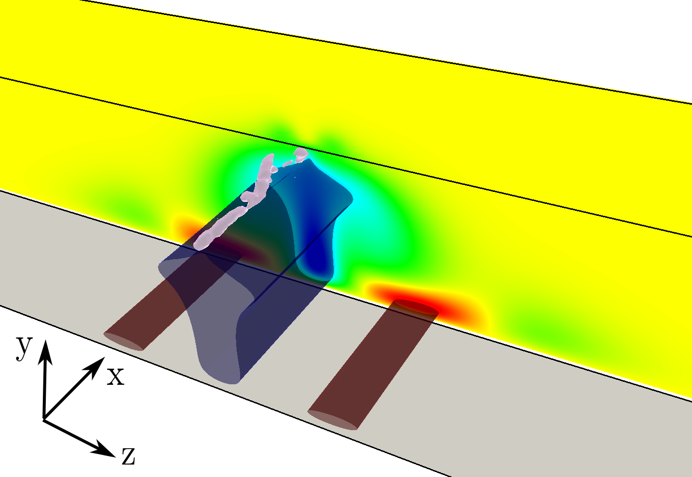
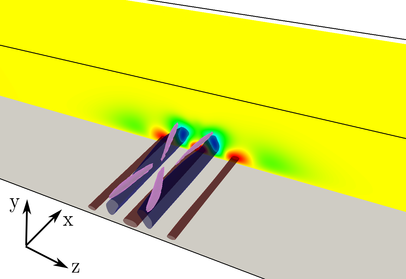
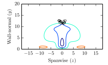
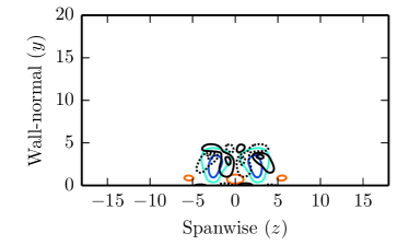
Figure 2: (a,b) Two localized equilibria of plane Couette flow, (a) EQ7-1 and (b) EQ7-2 from Gibson & Brand (2014) at $U_{\infty}H/\nu=1600$. Colours at the boundaries of the box show the streamwise-averaged deviation of streamwise velocity from the laminar profile. Isocontours of the $\lambda_{2}$ vortex detection criterion (Jeong & Hussain, 1995) are shown in purple. EQ7-1 has one pair of counter-rotating vortices, while EQ7-2 has two pairs. High and low-speed streaks are indicated by isocontours of the deviation of streamwise velocity from laminar flow: red for high-speed streaks (faster than laminar) and blue for low-speed streaks. (c,d) Free-stream coherent structure (FCS) and wall-mode (WM) travelling-wave solutions of the ASBL obtained by continuation from EQ7-1 and EQ7-2, with the same colour coding as in (a,b). (e,f) The roll-streak structures of the FCS and WM are indicated with isocontours of streamwise-averaged perturbation velocity $u$ (colours) and streamwise-averaged vorticity $\omega_{x}$ (solid black for positive $\omega_{x}$, dotted for negative). The FCS shown in (c,e) at $Re=1000$ consists of two weak high-speed streaks close to the wall and one low-speed streak that extends far into the free stream. The vortices are localized at $y\simeq 12$, far above the laminar boundary layer. The WM shown in (d,f) at $Re=400$ contains two pairs of vortices, two low- and three-high speed streaks, all within the laminar boundary layer, $y\leq\delta_{99\%}\simeq 5$,

Figure 2 compares the ASBL states to their progenitor states in plane Couette flow. Figure 2(a,b) shows EQ7-1 and EQ7-2 of plane Couette flow and (c,d) the corresponding FCS and WM states obtained by continuation to the ASBL, with vortices indicated by isosurfaces of $\lambda_{2}$ (Jeong & Hussain, 1995) in purple and velocity fluctuations by isosurfaces of streamwise velocity in blue and red (see figure caption for details). Figure 2(e,f) shows the roll-streak-structure of FCS and WM in the ASBL by isocontours of the downstream velocity (colours) and downstream vorticity (black). The first important observation is that both states are well-localized in the spanwise direction to within a range of $|z|<10$, considerably smaller than boundaries of the computational domain at $L_{z}/2=12\pi\simeq 38$ (see also figure 3).

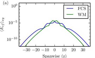
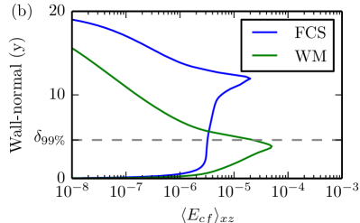
Figure 3: Localization properties of the FCS (blue) and WM (green) in the (a) spanwise and (b) wall-normal directions. Localization is indicated by the cross-flow energy $E_{cf}=v^{2}+w^{2}$ averaged in $x,y$ and $x,z$, respectively. The exponential drop-off in cross-flow energy with (a) $z$ and (b) $y$ confirms that the computational domain is sufficiently large. (b) The peak of cross-flow energy for the FCS is at $y\simeq 12$, far above the laminar boundary layer $y\leq\delta_{99\%}\simeq 5$, while for WM the peak is within it.

Like EQ7-1 in plane Couette flow, the FCS in the ASBL consists of a single pair of staggered and tilted counter-rotating vortices. These vortices are located at $y\simeq 12$, far above the laminar boundary layer thickness at $\delta=1$ or the laminar $99\%$ boundary layer thickness at $\delta_{99\%}=4.6$. Located below the vortices is a large low-speed streak, i.e. a region where the streamwise velocity is slower than in the surrounding laminar flow. The low-speed streak originates at the wall and ends below the vortices at $y\approx 12$, creating a small shear from which the vortices draw energy. Note that the streak contour lines are nearly as dense near the vortices as at the wall, indicating that the shear near the vortices is large, and that the large wall-normal extent of the low-speed streak in figure 2(e) is not an artifact of the choice of contour levels. Thus a key property of the FCS is that its vortices are sustained not by the laminar shear near the wall, but by shear far from the wall that the solution creates itself. The vortices push fluid to the sides by linear advection, creating a weak but large-scale circulation. This circulation pushes fluid from the free stream towards the wall on the right and left sides of the vortices, creating two weak high-speed streaks, and pulls fluid up in the center, creating the low speed-streak. The speed of the travelling wave is $c_{FCS}=0.905$, notably fast compared to the speed of turbulent spots in boundary layers (which travel at roughly $c=\frac{2}{3}$, Levin & Henningson (2007)) but consistent with the $1-c\sim 100\cdot O(\mbox{{Re}}^{-1})$ scaling estimated by DH14. Note that the laminar profile reaches this wavespeed ($u_{L}(y)=c_{FCS}$) at $y=2.35$.

There are several notable similarities between the spanwise-localized FCS figure 2 and the spanwise-periodic free-stream coherent structure of DH14. Both are derived from the EQ7 plane Couette solution of Gibson et al. (2009). The shift-reflect symmetry (6) of the FCS is the symmetry that remains after breaking the $z$-periodicity of the DH14 free-stream solution (their equation 3.4). Comparison of figure 2(e) with figure 3(e) of DH14 reveals similar structure and wall-normal position of the counter-rotating vortices of the two solutions, despite the differences in streamwise wavelength and Reynolds number ($L_{x}=4\pi,\mbox{{Re}}=968$ here versus $L_{x}=10\pi,\mbox{{Re}}=80,000$ in DH14). In both solutions the slow-speed streaks extend farther into the free stream than do the high-speed streaks, although for the DH14 free-stream solution, there is a clear concentration near the wall and decay away from it, whereas the low-speed streaks of the FCS have a more uniform core that extends farther into the free stream.

The WM in the ASBL is notably different from the FCS. The WM has two pairs of staggered, counter-rotating vortices much closer to the wall, below $y=\delta_{99\%}=4.65$. By linear advection (lift-up effect), the vortices create and sustain two low-speed and three high-speed streaks which are also very near the wall. The vortices are slightly tilted and inclined in the downstream direction, a pattern that is commonly observed in wall-bounded shear flows (Adrian, 2007). With all structures closely attached to the wall and the pattern of two vortices leaning over a low-speed streak, the WM is similar to the spanwise-localized edge states of Khapko et al. (2013), although in the latter, the crossing of the vortices over the streak destabilizes the streak, leading to breakup and reformation at a different position, and resulting in a time-dependent, relative periodic orbit solution. The speed of the WM travelling wave is $c_{WM}=0.87$, a speed reached by the laminar profile at $y=2.04$. The slower wavespeed of the WM compared to the FCS is consistent with its closer proximity to the wall. The WM is clearly related to the TW2-2 near-wall travelling wave of plane Poiseuille flow of Gibson & Brand (2014), both in their origin from EQ7-2 and in the structure of their vortices and streaks. How the WM relates to the wall mode of DH14 is less clear. The latter was continued from a different solution of sliding Couette flow and has vorticity concentrated much closer to the wall (comparing figure 2(d,e) to DH14 figure 3(b), albeit at different parameter values).

At a broad level, the FCS and the WM are composed of the same typical flow structures – streamwise streaks and downstream-oriented vortices – as almost all known invariant solutions in shear flows. The WM displays the familiar interactions known from the self-sustaining process (Hamilton et al., 1995; Waleffe, 1997; Schoppa & Hussain, 2002) or the vortex-wave interaction of Hall & Sherwin (2010). In the FCS, however, the strong vortices are not supported by a linear instability of the underlying streak (DH14), as complex nonlinear interactions dominate.

3.2 Dynamical properties of the free-stream coherent structure

In this section we show that the dynamical evolution of the FCS is detached from the wall. Figure 4 shows that the FCS has $O(10)$ unstable modes (eigenvalues with positive real part). The edge states of Khapko et al. (2013, 2014) in comparison have a single unstable eigenvalue by construction. Figure 5 shows the roll-streak structure of the four leading unstable eigenmodes. These are the most dynamically relevant eigenmodes, since they will dominate the evolution of trajectories that approach the FCS transiently. The leading eigenmodes are concentrated around the vortical structures of FCS at $y\simeq 12$, far from the wall. The linear dynamics near the FCS is thus concentrated near the free-stream part of the solution, and the streaks that extend close to the wall do not play a significant role.

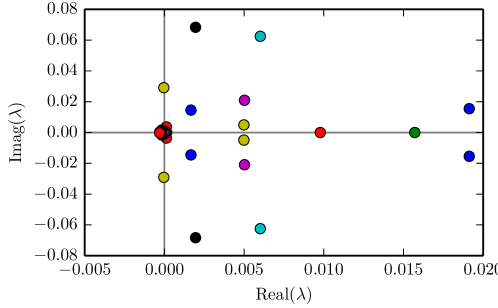
Figure 4: The leading eigenvalues of the FCS at $Re=1000$ with restriction to the shift-reflect symmetry subspace (6). With an increased resolution of $[64,121,576]$ grid points, the leading 10 eigenvalues differ by $10^{-4}$, confirming that the solution is well converged.

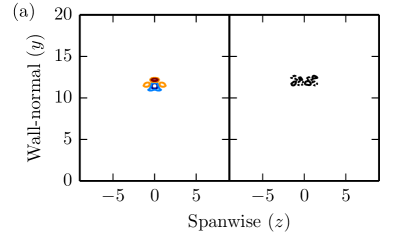
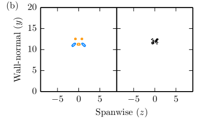
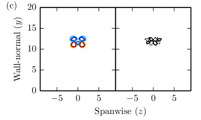
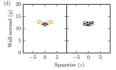
Figure 5: The four leading eigenmodes of the FCS. For complex eigenmodes, the real part is shown. The left part of each plot shows isocontours of the streamwise-averaged deviation of streamwise velocity from laminar flow, the right part the isocontours of streamwise-averaged streamwise vorticity. For all eigenmodes, the streaks and roll structures are localized in the free-stream, close to the vortices of the FCS.

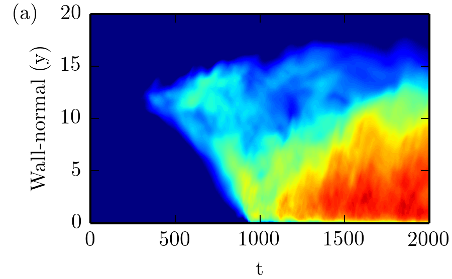
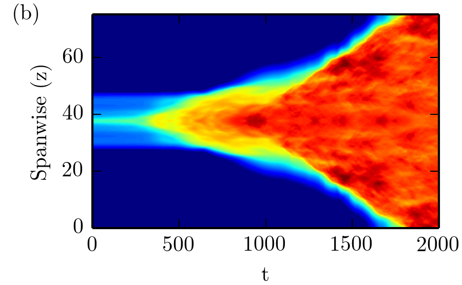
Figure 6: Space-time plots of the transition from FCS to turbulence at $Re=1000$. The averaged cross-flow energy $E_{cf}$ for the growth of a small perturbation of the FCS is shown as a function of time and the (a) wall-normal and (b) spanwise directions. The perturbation remains small for about $350$ advective time units. After $t\simeq 350$ the perturbations grow slowly in the spanwise direction and from the free stream towards the wall. When perturbations reach the laminar boundary layer $y\leq\delta_{99\%}$ around $t\simeq 800$, they strengthen and later spread rapidly along the wall, as shown by the increased slope of the red area in (b).

To study dynamics of transients near the FCS, we perturb the FCS slightly and follow the time evolution of the perturbed initial condition. Here we present results obtained by rescaling FCS by a factor of $1.01$; the qualitative results are unchanged if a small random perturbation is added instead. A movie in the supplementary material shows the evolution in time. Figure 6 shows space-time plots of the cross-flow energy $E_{cf}=v^{2}+w^{2}$ (Kreilos et al., 2013) as a function of $y$ and as a function of $z$, in each case averaged over the remaining two directions. No changes are visible for the first 350 time units as the exponential amplifications of the linearly unstable modes grow to large amplitudes. (This time of course depends on the magnitude of the initial perturbation). At $t\simeq 350$ velocity perturbations near the vortical structures at $y\simeq 12$ and $z=0$ grow to amplitudes comparable to the FCS velocity field. These perturbations spread in the $y$ direction mostly towards the wall and in the spanwise direction at roughly equal but slow propogation speeds. This slow spreading continues until the fluctuations reach the laminar boundary layer at $t\simeq 900$. After this, the fluctations strengthen and energetic turbulence begins to spread along the wall and also back into free stream. The rate of spanwise spreading is notably faster after the perturbations for $t\geq 1000$. This indicates that there are two different mechanisms by which turbulence spreads from the FCS: a slow growth of weak perturbations in the free stream followed by a faster, more energetic growth fueled by the shear of the laminar boundary layer.

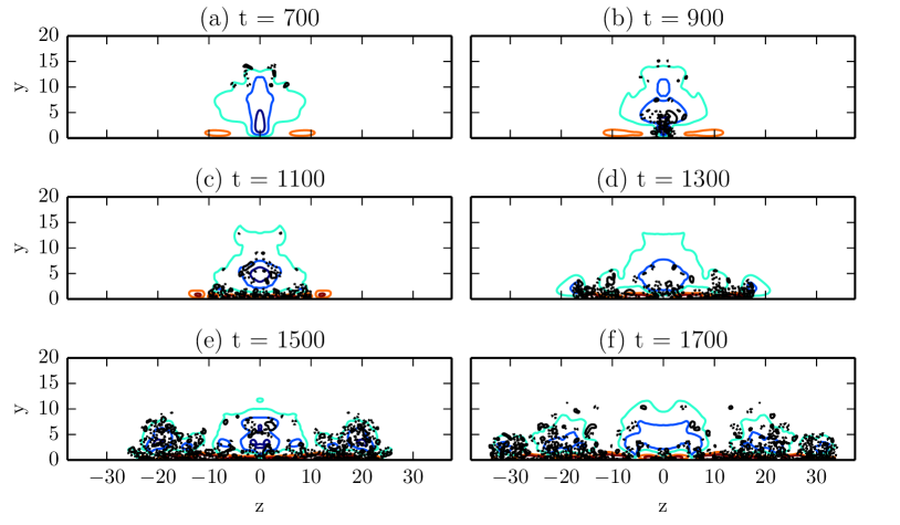
Figure 7: Time evolution of FCS, illustrating the spreading of weak perturbations towards the wall, followed by growth in energy and faster spreading in the spanwise direction. The plots show isocontours of the downstream velocity fluctuations in colours and isocontours of the downstream vorticity in black.

The observation that turbulence spreads rapidly once it reaches the wall is confirmed by the plots of the roll-streak structure in figure 7, with six snapshots of the trajectory taken at equidistant time intervals $\Delta t=200$. In panel (a) the state has not changed much from FCS and the vortical structures (black isocontours) are located high in the free stream. In panel (b) the perturbations have grown to the laminar boundary layer, where they are strongest. In panels (c-f) the stronger perturbations spread in the spanwise direction and start to grow in the wall-normal direction, creating a larger turbulent boundary layer, in which disturbances would ultimately grow to reach the upper boundary of the computational domain (Schlatter & Örlü, 2011).

4 Conclusions

We have presented two travelling wave solutions in the asymptotic suction boundary layer which are localized in both the wall-normal and the spanwise directions. This is the first time that spanwise-localized invariant solutions have been computed in a boundary layer. The wall-mode solution is closely attached to the wall, while the free-stream solution has vortices far from the wall, within the free stream. The vortices of the free-stream solution cannot draw energy from the laminar boundary layer; instead they are supported by a secondary shear gradient created by a large-scale, low-speed streak which stretches from the wall far into the free stream, convecting energy from the laminar gradient into the free-stream. The identification of this solution is thus an important step for invariant solutions in free-stream turbulence, as it shows the source of the shear gradient is not necessarily the background laminar flow profile, but can be a dynamical structure of the solution itself.

The localization of the free-stream solution’s unstable eigenfunctions and the dynamical evolution of perturbations from it show that the active region of this state is also detached from the wall. Perturbations of the free stream solution grow first around the vortical structures and then spread almost isotropically in the cross-stream plane, similar to a turbulent spot in a wall-parallel plane. Once the strong laminar shear at the wall is reached, the turbulent fluctuations sharply increase in magnitude and spread rapidly along the wall.