Active hydrodynamics of synchronization and ordering in moving oscillators

Abstract

The nature of emergent collective behaviors of moving physical agents interacting with their neighborhood is a long-standing open issue in physical and biological systems alike. This calls for studies on the control of synchronization and the degree of order in a collection of diffusively moving noisy oscillators. We address this by constructing a generic hydrodynamic theory for active phase fluctuations in a collection of large number of nearly phase-coherent moving oscillators in two dimensions. Our theory describes the general situation where phase fluctuations and oscillator mobility mutually affect each other. We show that the interplay between the active effects and the mobility of the oscillators leads to a variety of phenomena, ranging from synchronization with long range, nearly long range and quasi long range orders to instabilities and desynchronization with short range order of the oscillator phases. We highlight the complex dependences of synchronization on the active effects. These should be testable in wide ranging systems, e.g., oscillating chemical reactions in the presence of different reaction inhibitors/facilitators, live oriented cytoskeletal extracts, or vertebrate segmentation clocks.

I Introduction

The phenomenon of synchronization in which a large number of microscopic units spontaneously organize themselves into displaying cooperative behavior plays an important role in a wide class of systems, ranging from physics and biology to ecology, social dynamics and neurosciences pikovsky-book ; strogatz-book . Cooperative behavior in many living systems made of large number of living beings can be observed across a range of biological systems, e.g, a suspension of cells synchronizing their genetic clocks cells1 ; cells2 ; cells3 ; cells4 ; cells5 and flashing of fire flies fire-fly , and their artificial imitations arti-imi . For instance, when genetic oscillators that control the expression of a fluorescent protein is inserted in E. Coli bacteria, they can flash at a regular rate cells1 ; ecoli ; when coupled, a large population of bacteria can flash rhythmically in a synchronized manner cells2 ; cells4 . Two other notable relevant examples are vertebrate segmentation clock vertebrate and oscillating chemical reactions stirred-BZ .

The collective excitations in a large number of these nonequilibrium physical, chemical, and biological systems are in the form of cooperative oscillations of active interacting elements strogatz , e.g., chemical oscillators miyakawa-pre2002 ; toiya1 ; toiya2 ; fukuda-jphys ; kiss-prl ; migliorini ; strogatz-physicad ; BZ-vortical and synthetic genetic oscillators gen-osc , and biologically relevant systems frank22 ; frank-chiral ; sebastian ; liverpool ; frank-exp ; somitogenesis ; deve ; quorum ; Laskar . Spontaneous locking of interacting oscillators to a common phase dofler lead to synchronization of the oscillators, a ubiquitous collective behavior pikovsky-book ; strogatz-book , observed, e.g., in complex networks of phase oscillators dofler ; net1 . These call for studies on synchronization of a collection of locally interacting mobile oscillators. These have been studied extensively, in particular, in agent-based discrete systems frasca ; frank2 ; lauter ; pagona , where the network usually consists of a group of interacting moving oscillators. Equivalently, these model studies may also be viewed as examples of synchronization in dynamical networks, where the connectivity between any two oscillators evolves in time pagona ; chaos ; net1 . Recent studies on agent-based models with a large number of interacting mobile oscillators in one (1d) and two (2d) dimensions indicate that increasing the mobility of the oscillators significantly affect the steady states and may even lead to global synchronization frasca ; peruani . In addition, recent works provide evidence in favor of cell movement promoting synchronization of coupled genetic oscillators uriu1 ; uriu2 . Our work complement these existing studies. General understanding of how mobility of the oscillators affects synchronization (or, lack thereof) in a collection of mobile oscillators form the principal motivation of this work.

In this article, we focus on the the generic long wavelength properties of small fluctuations in a collection of diffusively mobile, nearly phase-coherent, noisy out-of-equilibrium oscillators in 2d. We introduce a generic active hydrodynamic theory for such systems. We analyze the broken symmetry phase fluctuations of these oscillators in their nearly phase coherent states and examine the general conditions for synchronization. Hydrodynamic approaches are distinguished by their generality of predictions and have been successfully applied to the ordered broken symmetry phases of many equilibrium and nonequilibrium systems martin-parodi-pershan ; active-fluid . Hydrodynamic theories are particularly suitable to extract statistical properties in the limit of large distance and long time scales  martin-parodi-pershan ; active-fluid . In order to generalize the scope of our study, we study a collection of large number of diffusively mobile oscillators in the continuum limit, where the local phase and number density fluctuations can mutually affect each other. In other words, in a discrete, agent-based description, the agents undergo persistent random walk that depends on the local phase fluctuations affect . The active interplay between the oscillator phases and the oscillator mobility is shown to control the degree of phase coherence. This forms the principal result of this work. Our model provides a generic long wavelength description for active mobility-induced synchronization frasca ; peruani ; markus ; mobility in 2d with the additional feature that the mobility is affected by local phase fluctuations. We expect it to be relevant in experiments pertaining to a wide class of systems, ranging from oscillating chemical reactions b-z ; b-r ; b-l ; i-c in the presence of catalysts to vertebrate segmentation clocks vertebrate ; deve ; frank2 , oriented live cytoskeletal extracts sebastian and clock synchronization in mobile robots chaos as well as help in designing new artificial imitations arti-imi . Our work generalizes studies on synchronization in complex dynamical network frasca ; pagona ; peruani ; net1 ; affect , where the time-evolution of the network is affected by the oscillator phases.

In order to concentrate on the essential physics of phase fluctuations and ordering lauter , we study the active stochastic dynamics of a collection of diffusive particles of concentration $c({\bf x},t)$ in 2d on a rigid substrate, each carrying oscillators in their nearly phase-coherent state. The oscillators are represented by a complex field $Z=\exp[i\phi({\bf x},t)]$ with unit amplitude and phase $\phi$ at point $\bf x$ and time $t$, and have the same internal symmetry as the XY model classicalxy . In stark contrast to related 2d equilibrium systems with XY symmetry, we show that this model displays a wide class of behaviors, ranging from synchronization with long range order (LRO), quasi-long range order (QLRO) and nearly long range order (NLO) to linear instability with desynchorinization and short range order (SRO), and nonlinear stabilization of linear instability. These are controlled by the interplay between active effects and particle diffusivity. In analogy with thermally excited systems, these regimes with different natures of order are characterized by the analog of the Debye-Waller factor $\sim\exp(-\Delta)$, where $\Delta=\langle\phi({\bf x},t)^{2}\rangle$ ($\langle...\rangle$ implies averages over the noises) classicalxy ; o_n ; comment-debye . Here, $\Delta$ provides a measure of order or degree of phase synchronization: for a given $L$, where $L$ is the system size, the smaller $\Delta$ is, the higher is the order or the degree of synchronization. In particular, in the linearly stable regime and in the limit of fast concentration relaxation (also called fast switching regime, see below), $\Delta$ can be reduced by enhancing (positive) $\gamma$, the active damping of phase fluctuations, with either LRO (finite $\Delta$) or NLO ($\Delta$ varying as $\ln\ln L$) in the system. For negative $\gamma$, linear instability ensues, implying SRO or desynchronization. Additionally, in some cases formation of patterns are predicted. Our work reveals complex dependences of phase fluctuations of a collection of moving oscillators on active effects. The rest of the article is organized as follows: In Sec. II we construct our model and describe the origin of the active terms. Then in Sec. III we discuss our results for both the linear and nonlinear theories. Finally, in Sec. IV we summarize and conclude. An Appendix containing some calculational details has been added at the end for helping the readers.

II Construction of the model equations

We consider small fluctuations about a uniform phase-coherent reference state with a constant concentration $c_{0}$ and a uniform phase of the oscillators. We now construct the generic coupled hydrodynamic equations for the two slow variables - local fluctuations $\phi({\bf x},t)$ in the phase and concentration fluctuations $\delta c({\bf x},t)=c({\bf x},t)-c_{0}$. We allow for advection of $\phi$ and $c$ by an incompressible velocity $\bf v$. Field $\phi$ being the phase fluctuations in a phase-coherent state, is a nonconserved broken symmetry variable, whereas $\delta c$ is a conserved density. These considerations together with symmetry arguments (invariance under translation, rotation and a spatially constant shift $\phi\rightarrow\phi+const.$) dictate the general forms of the equations of $\phi$ and $\delta c$. The most general coupled dynamical equations for $\phi$ and $\delta c$, where they mutually affect each other, are of the form

$$\frac{\partial\phi}{\partial t}+\frac{\lambda}{2}({\boldsymbol{\nabla}}\phi)^{2}+\lambda_{1}{\bf v}\cdot{\boldsymbol{\nabla}}\phi=\tilde{\Omega}(c)+\kappa\nabla^{2}\phi+\theta,$$ (1)

$$\frac{\partial\delta c}{\partial t}+\lambda_{1}{\bf v}\cdot{\boldsymbol{\nabla}}\delta c=D_{c}\nabla^{2}\delta c+\lambda_{2}\nabla^{2}\phi+{\boldsymbol{\nabla}}\cdot{\bf f},$$ (2)

in the hydrodynamic limit. Terms $\lambda({\boldsymbol{\nabla}}\phi)^{2},\tilde{\Omega}(c)$ in (1) and $\lambda_{2}\nabla^{2}\phi$ in (2) are active terms, i.e., of nonequilibrium origin. These are forbidden in equilibrium due to the invariance of an underlying free energy functional $\mathcal{F}$ under $\phi\rightarrow\phi+const.$. In the present model, this invariance must be demanded at the level of the equations of motion and hence the above active terms are permitted in (1) and (2) argument . In Eq. (1), we have neglected a subleading cross-coupling term of the form $\sim\nabla^{2}\delta c$ in the hydrodynamic limit; see below. Equations (1) and (2) generalize the nonconserved relaxational dynamics of the local phase of the nearly phase coherent classical XY model; parameter $\kappa>0$ is the analog of the spin stiffness of the classical XY model classicalxy . The $\lambda_{1}$-terms in (1) and (2) above represent advection by $\bf v$, and the $\lambda$-term in (1) is a nonequilibrium term related to the well-known complex Ginzburg Landau model cgle ; erwin-cgle or the dissipative Gross-Pitaevskii equation for a polariton condensate polariton . Expanding about $c=c_{0}$, we write

$$\tilde{\Omega}(c)=\tilde{\Omega}_{0}+\tilde{\Omega}_{1}\delta c+\tilde{\Omega}_{2}(\delta c)^{2}+\tilde{\Omega}_{3}(\delta c)^{3},$$ (3)

neglecting other higher order terms. Parameters $\tilde{\Omega}_{1},\tilde{\Omega}_{2},\tilde{\Omega}_{3}$ can be positive or negative; without any loss of generality we set $\tilde{\Omega}_{1}>0$. Parameters $\lambda,\lambda_{1}$ and $\kappa$, in general functions of $c$, upon expanding about $c=c_{0}$, yield additional nonlinear terms that are subleading in a scaling sense (i.e., leave the scaling properties unaffected). Hence, we ignore their $c$-dependences. In the limit of spatially constant $c$, $\tilde{\Omega}(c)$ may be absorbed by a frequency shift, that yields, for ${\bf v}=0$, the Kardar-Parisi-Zhang (KPZ) equation for $\phi$ kpz . Additionally, if $\lambda=0$, Eq. (1) reduces to the standard relaxational equation of motion for the phase in the classical XY model classicalxy . For $\lambda_{2}=0$, $\delta c$ follows a diffusion-advection equation, independent of $\phi$; with $\lambda_{2}\neq 0$, the particle mobility is deemed active. Equation (2) implies a concentration current

$${\bf J}_{c}=-\left[D_{c}{\boldsymbol{\nabla}}\delta c-\lambda_{1}{\bf v}\delta c+\lambda_{2}{\boldsymbol{\nabla}}\phi+{\bf f}\right].$$ (4)

Noises $\theta$ and $\bf f$ noise2 are zero-mean Gaussian-distributed with variances $\langle\theta({\bf x},t)\theta(0,0)\rangle=2D\delta({\bf x})\delta(t)$ and $\langle f_{\alpha}({\bf x},t)f_{\beta}(0,0)\rangle=2D_{1}\delta_{\alpha\beta}\delta({\bf x})\delta(t)$, respectively; in a nonequilibrium situation, $D,\,D_{1}$ have dimensions of temperature $T$ and are in general unequal. We have ignored cross-coupling terms of purely equilibrium origin in Eqs. (1) and (2) above as they are irrelevant (in a scaling sense) to the active terms in (1) and (2) in the long wavelength limit. Equations (1) and (2) generalize the relaxational dynamics of the classical XY model to any active system having XY symmetry with mobility.

For a frictional flow, $\bf v$ follows generalized Darcy’s law darcy , that here includes the leading order symmetry-permitted feedback of $\phi$ on $\bf v$ o_n ; modelH ,

$$-\zeta v_{\alpha}=\alpha_{0}P_{\alpha\beta}\frac{\partial}{\partial x_{\gamma}}(\frac{\partial\phi}{\partial x_{\gamma}}\frac{\partial\phi}{\partial x_{\beta}})+P_{\alpha\beta}g_{\beta}.$$ (5)

Here, $P_{\alpha\beta}=\delta_{\alpha\beta}-\frac{\nabla_{\alpha}\nabla_{\beta}}{\nabla^{2}}$ is the transverse projection operator and $\zeta$ is a friction coefficient addicomment . For a nonequilibrium model, coupling $\alpha_{0}$ has no restrictions on its sign o_n . Noise $g_{\alpha}$ is a zero-mean, Gaussian white noise with a variance $\langle g_{\alpha}({\bf x},t)g_{\beta}(0,0)\rangle=2D_{3}\zeta\delta_{\alpha\beta}\delta({\bf x})\delta(t)$. $D_{3}$ again has the dimension of temperature.

II.1 The active terms

We now discuss the origin and physics of the active terms in more details. In Eq. (1), if we ignore the time-dependence of $\delta c$, the function $\tilde{\Omega}(c)$ becomes the natural frequency of the oscillator. This, in a discrete lattice-gas representation, implies that the natural frequency of a particular oscillator is nonuniform and a local property, i.e., it depends upon the number of the oscillators in its neighborhood. This is a generalization of the well-known Kuramoto model for identical phase oscillators (i.e., with the same natural frequency) kuramoto1 ; kuramoto2 . Depending upon the function $\tilde{\Omega}(c)$, an oscillator either rotates faster or slower as the number of oscillators in its neighborhood changes. Consider now the other active term $\lambda_{2}\nabla^{2}\phi$ in (2). This corresponds to a current contribution $-\lambda_{2}{\boldsymbol{\nabla}}\phi$ in ${\bf J}_{c}$. Thus, neighboring oscillators will move towards or go away from each other if there is a phase difference between them, constituting an active, $\phi$-dependent current with a magnitude set by $\lambda_{2}$. Depending on the sign of $\lambda_{2}$, this active current either reinforces or goes against the usual diffusive current $D_{c}{\boldsymbol{\nabla}}\delta c$.

In the equilibrium limit, the system may be described by a free energy $\mathcal{F}$ given by

$${\mathcal{F}}=\int d^{2}x[\frac{\kappa}{2}({\boldsymbol{\nabla}}\phi)^{2}+A\delta c\nabla^{2}\phi+\frac{B}{2}(\delta c)^{2}].$$ (6)

Here, $A$ and $B$ are thermodynamic coefficients. The sign of $A$ is arbitrary, while $B$ is always positive. Free energy (6) yields (assuming simple relaxational dynamics, ignoring any advection for simplicity)

$$\frac{\partial\phi}{\partial t}=-\frac{\delta{\mathcal{F}}}{\partial{\mathcal{\phi}}}+\theta=-[-\kappa\nabla^{2}\phi+A\nabla^{2}\delta c]+\theta,$$ (7)

and

$$\frac{\partial\delta c}{\partial t}=\nabla^{2}\frac{\delta{\mathcal{F}}}{\delta(\delta c)}+\boldsymbol{\nabla}\cdot{\bf f}=B\nabla^{2}\delta c+A\nabla^{4}\phi+{\boldsymbol{\nabla}}\cdot{\bf f}.$$ (8)

The linear cross terms are clearly subleading to the active terms $\tilde{\Omega}_{1}(c)$ and $\lambda_{2}\nabla^{2}\phi$ in Eqs. (1) and (2) above. In fact, if we insist on generating these active terms from $\mathcal{F}$, we may consider adding terms, e.g., of the form $\tilde{\Omega}_{1}(c)\phi$ in $\mathcal{F}$, that generates a term $\tilde{\Omega}(c)$ in Eq. (1) of the main text, but manifestly breaks the invariance under $\phi\rightarrow\phi+const.$, which is not acceptable. This establishes the active origin of the term $\tilde{\Omega}_{1}(c)$ and similarly of $\lambda_{2}\nabla^{2}\phi$ in Eqs. (1) and (2), respectively, above.

Equations (1) and (2) serve as good representations for different real systems. Consider a 2d array of identical water droplets, which contain the reactants of an oscillatory chemical (e.g., Belousov-Zhabotinsky) reaction, separated by oil gaps; see, e.g., Ref. toiya1 , with $\phi$ and $c$, respectively, being the phase of the oscillatory reaction and catalyst concentration. Or consider a layer of oriented chiral live cytoskeletal acto-myosin extract resting on a solid substrate. For fully oriented actin filaments (in the limit of large Frank’s constant jacques-book , or for length scales smaller than the threshold of spontaneous flow instabilities rafael ), polarity fluctuations may be neglected, and $\phi$, that describes chirality of actin and $c$, the concentration of actin filaments are the slow variables. In yet another general biological motivation of our theory, the vertebrate segmentation clocks, $\phi$ and $\delta c$ represent, respectively, the local phases of genetic oscillations and the concentration of the migrating cells or the signaling molecules vertebrate . In all these examples, active terms $\tilde{\Omega}(c)$ in (1) and $\lambda_{2}{\boldsymbol{\nabla}\phi}$ in current ${\bf J}_{c}$ model generic active interplay between phase and concentration fluctuations. In general, all the active coefficients $\lambda,\tilde{\Omega}_{0},\tilde{\Omega}_{1},\tilde{\Omega}_{2},\tilde{\Omega}_{3},\lambda_{2}$ should depend on $c_{0}$, the mean concentration of the diffusing active particles. Diffusivity $D_{c}$ should contain both thermal (equilibrium) and active contributions; see, e.g., Ref. abhik-diff .

We now compare our model equations with those that describe active fluid with orientational degrees of freedom, viz., the equations of the local polar order parameter or orientation field $\bf p$ and the concentration of the active particles active-fluid ; john . While both the systems are concerned with the question of order in 2d, there are notable differences between the two. Our model equation (1) that generalizes the Kuramoto model equation, necessarily applies to phases of oscillators or rotors, i.e., to microscopic oscillatory degrees of freedom. Such a collection of oscillators has no notion of local orientation or polarity in the physical space. This is quite different from the active fluids active-fluid ; john , where the local polarity describes local orientation of the underlying polar or nematic degrees of freedom (i.e., actin filaments, birds or fishes). Furthermore, polar ordered active fluids are generically characterized by systematic macroscopic motion along the direction of order, where as the oscillators considered here are diffusively moving, devoid of any systematic large-scale movement. The one particular case of active fluid models where our model should be relevant is chiral active fluids, where the actin filaments have chirality given by a phase variable sebastian . A fully orientationally ordered chiral active fluid with very large Frank’s constants (that suppress any orientational fluctuations) without any large scale motion should be described only by the phase and the local concentration of the active particles. For such a system our model equations should form a valid description. Lastly, the ordered state of an active fluid is necessarily anisotropic due to the macroscopic preferred orientation across the system. In contrast, a globally synchronized state of phase oscillators like ours is perfectly isotropic in the physical space.

III Results

III.1 Fast switching regime

III.1.1 Linear theory

We now analyze Eqs. (1) and (2) to ascertain the degree of global synchronization in the model. It is illuminating to first consider the linearized version of Eqs. (1) and (2). We linearize Eq. (1) about $c=c_{0}$, and define time scales $\tau_{\phi}(q)=1/(\kappa q^{2})$ and $\tau_{c}(q)=1/(D_{c}q^{2})$, where $\bf q$ is a Fourier wavevector; thus $\tau_{\phi}$ is the time-scale of isolated phase fluctuations (i.e., in the absence of any coupling with $c$), where as $\tau_{c}$ is the time-scale in which isolated particles diffuse, or the network evolves. Now eliminate $\delta c$ in (1) to obtain (in the Fourier space)

$$-i\omega\phi=-\kappa q^{2}\phi-\frac{\lambda_{2}\tilde{\Omega}_{1}q^{2}}{-i\omega+D_{c}q^{2}}\phi+\frac{i\tilde{\Omega}_{1}{\bf q\cdot f}}{-i\omega+D_{c}q^{2}}+\theta.$$ (9)

Here, $\omega$ is the Fourier frequency. The two time-scales $\tau_{\phi}$ and $\tau_{c}$ can compete with each other with two asymptotic limits $\tau_{\phi}\gg\tau_{c}$ (fast switching regime in the network language pagona ) and $\tau_{\phi}\ll\tau_{c}$ (slow switching regime). We note that recent studies on synchronization in 1d using agent based models peruani indicate that large oscillator diffusivities tend to enhance the degree of global synchronization. A large $D_{c}$ implies a small $\tau_{c}(q)$ for fixed $q$. Taking cue from this and in order to extract the activity-dependence of synchronization in the most dramatic way, we consider the limit $D_{c}\rightarrow\infty$, or equivalently, $\tau_{c}\rightarrow 0$; clearly $\tau_{c}\ll\tau_{\phi}$ for a finite $\kappa$. In this limit, Eq. (9) simplifies to (in the time domain)

$$\frac{\partial\phi}{\partial t} = -\kappa q^{2}\phi-\frac{\tilde{\Omega}_{1}\lambda_{2}}{D_{c}}\phi+\theta+\frac{i{\bf q}\cdot{\bf f}\tilde{\Omega}_{1}}{q^{2}D_{c}}$$ (10)

$$= -\kappa q^{2}\phi-\gamma\phi+\theta+\frac{i{\bf q}\cdot{\bf f}\tilde{\Omega}_{1}}{q^{2}D_{c}},$$

where $\gamma=\tilde{\Omega}_{1}\lambda_{2}/D_{c}$ is an active coefficient. Equation (10) allows us to extract yet another time-scale $\tau_{\times}=\frac{D_{c}}{\tilde{\Omega}_{1}\lambda_{2}}=\frac{1}{\gamma}$ ($\gamma$ has the dimension of inverse time); $\tau_{\times}$ is infact the time-scale of phase fluctuations due to the active coupling of $\phi$ with concentration fluctuation $\delta c$. We assume $\gamma\sim O(1)$, i.e., $\tau_{c}/\tau_{\times}\rightarrow 0$. (Note that for $\gamma$ to dominate the long wavelength dynamics of $\phi$, $|\gamma|>\frac{4\pi^{2}\kappa}{L^{2}}$. We present most of our results in this limit. This is realizable for large enough $L$ with sufficiently large $\tilde{\Omega}_{1}\lambda_{2}$.) Since active coefficients $\tilde{\Omega}_{1}$ and $\lambda_{2}$ are formally independent of $D_{c}$, this can be realized by letting $\tilde{\Omega}_{1}\lambda_{2}\rightarrow$ large with a large $D_{c}$. Notice that in this fast switching regime, the dynamics of $\delta c$ is effectively slaved to $\phi$. We now set out to calculate $\Delta$ below in the limit of fast dynamics of $\delta c$.

Evidently for a positive $\tilde{\Omega}_{1}$, Eq. (10) is linearly unstable if active damping $\gamma<0$ ($|\gamma|$ : growth rate); i.e., if $\lambda_{2}<0$; else, it is linearly stable ($\gamma$ : decay rate). For a positive $\tilde{\Omega}_{1}$, thus, $\lambda_{2}>0(<0)$ implies that any local excess of diffusive species reduces (enhances) any local nonuniformity in $\phi$ micro1 .

Now, consider

$$\Delta=\int_{1/L}^{\Lambda}\frac{d^{2}q}{(2\pi)^{2}}\langle|\phi({\bf q},t)|^{2}\rangle=\int_{1/L}^{\Lambda}\frac{d^{2}q}{(2\pi)^{2}}\frac{d\Omega}{2\pi}\frac{\langle|\theta|^{2}+|f^{\prime}|^{2}\rangle}{\Omega^{2}+\gamma^{2}}$$ (11)

for $\gamma>0$ in the linearized theory together with $\tau_{c}\rightarrow 0$ and $\tau_{\times}\sim O(1),\tau_{c}/\tau_{\times}\rightarrow 0$. Here, $f^{\prime}=\frac{\tilde{\Omega}_{1}iq_{\alpha}f_{\alpha}}{q^{2}D_{c}}$, $\phi({\bf q},t)$ is the Fourier transform of $\phi({\bf x},t)$. We define a length scale $L_{c}$ given by the relation

$$\frac{D_{1}\tilde{\Omega}_{1}^{2}}{D_{c}^{2}D}=1/L_{c}^{2}.$$ (12)

Since $L_{c}$ depends explicitly on the active coefficient $\tilde{\Omega}_{1}$, it can be tuned by the active processes. In particular, $L_{c}$ can be made very large for small $\tilde{\Omega}_{1}$. The nature of order depends sensitively on the dimensionless ratio $L/L_{c}$, as we establish below.

For $\frac{L}{L_{c}}\ll 1$, this yields

$$\Delta=\int_{1/L}^{\Lambda}\frac{d^{2}q}{(2\pi)^{2}}\frac{d\omega}{2\pi}\frac{\langle|\theta|^{2}\rangle}{\omega^{2}+\gamma^{2}}\approx\frac{D\Lambda^{2}}{2\pi\gamma},$$ (13)

for $L\gg 1/\Lambda$. Notice that this $L$-independence of $\Delta$ holds even in 1d. In contrast for large $\frac{L}{L_{c}}\gg 1$,

$$\Delta=\int_{1/L}^{\Lambda}\frac{d^{2}q}{(2\pi)^{2}}\frac{d\omega}{2\pi}\frac{\langle|f^{\prime}|^{2}\rangle}{\omega^{2}+\gamma^{2}}\approx\frac{D}{2\pi L_{c}^{2}\gamma}\ln L,$$ (14)

for $L\gg 1/\Lambda$. Here, $\Lambda$ is an upper wavevector cut-off, $\omega$ is a frequency remark_2 . See Fig. 1 for a schematic phase diagram (with $\gamma>0$) in the $L_{c}-L$ plane, showing regions corresponding to LRO and QLRO, respectively.

Figure 1: Behavior of $\Delta$ in the $L_{c}-L$ plane in the linear theory (with $\gamma>0$) in the fast switching regime. The straight line refers to $L=L_{c}$; see text.

The nature of order can be established from the equal-time oscillator correlator o_n

$$C_{s}(r)=\langle\cos[\phi({\bf x},t)-\phi(0,t)]\rangle=\exp[-g(r)]$$ (15)

for large $r=|\bf x|$ with $g(r)=\langle[\phi({\bf x},t)-\phi(0,t)]^{2}\rangle/2$. This yields

$$g(r)=D\Lambda^{2}/(2\pi\gamma),$$ (16)

for large $r$ (with $r\lesssim L<L_{c}$), demonstrating LRO. Thus, for a system of size $L\ll L_{c}$ and $\gamma>0$, the system can show LRO in the fast switching regime, such that $L\ll L_{c}$; see Refs. frasca and peruani which show numerically how increasing mobility can lead to global synchronization. Notice that in our model $L_{c}$ may be made arbitrarily large even with a large $D_{c}$ by adjusting the other model parameters; see Eq. (12) above. In contrast, for large $r$ with $L_{c}<r<L$,

$$g(r)=\frac{D}{2\pi L_{c}^{2}\gamma}\ln r,$$ (17)

hence, showing QLRO in the system o_n . For $\gamma<0$, only for a finite system size with $L^{2}<4\pi^{2}\kappa/|\gamma|$, $\Delta$ is finite, implying SRO peruani . This allows us to define a persistence length $\xi_{1}$, given by

$$\xi_{1}=2\pi(\kappa/|\gamma|)^{1/2},$$ (18)

such that for $L>\xi_{1}$, instability ensues. Thus given the activity-dependences of $\gamma$ and $L_{c}$, the role of active effects in facilitating or destroying order is clearly established. Evidently, the larger $|\gamma|$ is, the stronger is the linear instability ($\gamma<0$) or stronger suppression of phase fluctuations (more stable, $\gamma>0$); see Fig. 2 for a schematic phase diagram in the $\lambda_{2}-\tilde{\Omega}_{1}$ plane. Since all of $D_{c},\tilde{\Omega}_{1}$ and $\lambda_{2}$ are expected to scale with $C_{0}$, the mean concentration, $\gamma$ should scale with $C_{0}$. Thus any activity-induced synchronization or instability should be enhanced in a denser system - a broad feature testable in experiments on relevant systems.

Figure 2: Schematic phase diagram in the $\lambda_{2}-\tilde{\Omega}_{1}$-plane showing linearly stable and unstable regions in the linear theory in the fast switching regime; see text. Symbol $O$ marks the origin $(0,0)$.

III.1.2 Nonlinear effects

We now consider the dominant nonlinear effects on the results from the linear theory. For 2d equilibrium systems with continuous symmetries in their ordered phases, this is most conveniently done in terms of a low-$T$ expansion in 2D, where a dimensionless reduced $T$ (assumed small in the putative ordered phases) plays the role of a small parameter classicalxy . This has subsequently been extended to analogous nonequilibrium systems, see, e.g., Ref. o_n . Following Ref. o_n , we identify $D\Lambda^{2}/\gamma$ and $D/(L_{c}^{2}\gamma)$ as the dimensionless small parameters and restrict ourselves up to their linear order expansions, for (assumed) small fluctuations of $\phi$ and $v_{\alpha}$ with $\tau_{c}/\tau_{\times}\rightarrow 0$. We replace $\tilde{\Omega}_{3}(\delta c)^{3}$ in Eq. (3) by a linear term $3\tilde{\Omega}_{3}\langle(\delta c)^{2}\rangle\delta c$ in a Hartree-like approximation classicalxy and substitute it in Eq. 1. This then produces a correction $\overline{\gamma}$ to $\gamma$. With $\gamma>0$, following our analysis at the linear order above, we define an effective active damping coefficient

$$\gamma_{e}=\gamma+\overline{\gamma},$$ (19)

where $\overline{\gamma}=\frac{3\tilde{\Omega}_{3}\langle(\delta c)^{2}\rangle\lambda_{2}}{D_{c}}$.

Now, in the linear theory with $\tau_{c}\rightarrow 0$ and $\tau_{c}/\tau_{\times}\rightarrow 0$, such that the dynamics of $\delta c$ is slaved to that of $\phi$,

$$\delta c=-\frac{\lambda_{2}}{D_{c}}\phi+\frac{i{\bf q\cdot f}\tilde{\Omega}_{1}}{D_{c}q^{2}}.$$ (20)

Equation (20) may now be used to calculate $\langle|\delta c({\bf q},t)|^{2}\rangle$ separately for $L<L_{c}$ and $L>L_{c}$, since the form of $\langle|\phi({\bf q},t)|^{2}\rangle$ depends on whether $L<L_{c}$ or $L>L_{c}$.

(i) For $L<L_{c}$,

$$\langle\delta c^{2}\rangle=\frac{\lambda_{2}^{2}}{D_{c}^{2}}\int_{1/L}^{\Lambda}\frac{d^{2}q\,d\Omega}{(2\pi)^{3}}\frac{D}{\gamma}\approx\frac{\lambda_{2}^{2}D\Lambda^{2}}{4\pi\gamma D_{c}^{2}}.$$ (21)

Using this value of $\langle(\delta c)^{2}\rangle$ the correction to $\gamma$ takes the form

$$\overline{\gamma}=3\tilde{\Omega}_{3}\lambda_{2}^{2}D\Lambda^{2}/(4\pi D_{c}^{2}\tilde{\Omega}_{1}),$$ (22)

which is finite. For $\tilde{\Omega}_{3}>0$, we have $\overline{\gamma}>0$, thus leaving the results from the linear theory qualitatively unchanged. On the other hand, for $\tilde{\Omega}_{3}<0$, this correction is negative and has the potential of introducing instability provided $|\overline{\gamma}|>\gamma$. This yields a finite instability threshold for $|\tilde{\Omega}_{3}|$, given by $\tilde{\Omega}_{3}^{c}=\frac{4\pi\gamma\tilde{\Omega}D_{c}^{2}}{3\Lambda^{2}\lambda_{2}^{2}D}$.

(ii) For $L\gg L_{c}$, $\overline{\gamma}\approx\Gamma\ln L$, diverging logarithmically with $L$;

$$\Gamma=3\tilde{\Omega}_{3}\lambda_{2}^{2}\tilde{\Omega}_{1}D_{1}/(2\pi D_{c}^{4}),$$ (23)

see Appendix. Thus, $\overline{\gamma}$ necessarily dominates over $\gamma$ for sufficiently large $L$; thence, for $\tilde{\Omega}_{3}<0$ and $\gamma>0$ the instability necessarily sets in for a sufficiently large $L$, without any finite threshold for $\tilde{\Omega}_{3}$. This nonlinearity induced instability allows us to introduce a modified persistence length

$$\tilde{\xi}_{1}=2\pi(\kappa/|\gamma_{e}|)^{1/2},$$ (24)

now controlled by $\tilde{\Omega}_{3}$ for a fixed $\gamma>0$. Similar to the calculations for the linear theory, now with $\gamma_{e}>0$, we find for large $r\lesssim L<L_{c}$, $g(r)=D\Lambda^{2}/(2\pi\gamma_{e})$. This confirms LRO as in the linear theory (see above). On the other hand, for large $r>L_{c}$, $g(r)=\overline{A}\ln\ln r$, showing that $C_{s}(r)$ decreases as $1/(\ln r)^{\overline{A}}$; $\overline{A}=D_{1}\tilde{\Omega}_{1}^{2}/(\Gamma D_{c}^{2})$. Thus in this case, QLRO in the linear theory gets modified to NLO by the nonlinear effects with a spatial decay slower than the algebraic decay in QLRO o_n . For $\gamma<0$ ($\lambda_{2}<0$), linear instability ensues. However, nonlinear effects can stabilize and suppress this linear instability, provided $\tilde{\Omega}_{3}>0$ and $\overline{\gamma}>|\gamma|$. Therefore, depending on the signs of $\lambda_{2}$ and $\tilde{\Omega}_{3}$, four distinct possibilities emerge, as shown in Fig. 3 schematically in the $\tilde{\Omega}_{3}-\gamma$ plane.

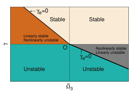
Figure 3: (Color online) Schematic phase diagram in $\tilde{\Omega}_{3}-\gamma$ plane ($\zeta>0$). Symbol $O$ refers to the origin $(0,0)$. Regions (i) linearly and nonlinearly stable (both $\gamma,\gamma_{e}>0$), (ii) linearly stable, nonlinearly unstable ($\gamma>0,\gamma_{e}<0$), (iii) linearly unstable, nonlinearly stable ($\gamma<0,\gamma_{e}>0$) and (iv) linearly and nonlinearly unstable (both $\gamma,\gamma_{e}<0$) are marked (see text). The inclined lines, drawn schematically, are to be obtained from the conditions $\gamma_{e}=0$.

The advective nonlinearities in Eqs. (1) and (2) generate additional corrections to the model parameters in Eqs. (1) and (2). This is acheived by eliminating $\bf v$ in Eq. (1) with the help of Eq. (5), which generates finite corrections to $\kappa$ and $\gamma$ for both $L<L_{c}$ and $L>L_{c}$. See Appendix for some calculational details regarding advective nonlinearities.

For $\lambda_{1}\alpha_{0}$ sufficiently negative, $\gamma_{e}$ and $\kappa_{e}$ that now include additional corrections from $\lambda_{1}$, may become negative and thus lead to long wavelength instabilities and pattern formations. For instance, for $\gamma_{e}>0$ and $\kappa_{e}<0$, finite wavevector instabilities are produced in the system at $O(q^{2})$, while remaining stable at $O(q^{0})$. The instability at $O(q^{2})$ for $\kappa_{e}<0$ should be suppressed at very high $q$ by a stabilizing generic fourth order spatial derivative term $-\kappa_{4}\nabla^{4}\phi(\kappa_{4}>0)$ in the rhs of Eq. (1) (here neglected; see Ref. lauter ). For $\lambda_{1}\alpha_{0}>0$, these corrections do not affect the scaling of $\Delta$. The regions in phase space where $\kappa_{e}$ is negative should display patterns in the steady state. Our hydrodynamic theory, based on retaining only the lowest order gradients and low order nonlinear terms cannot determine the steady state patterns. The detailed nature of the patterns should depend upon the higher order terms neglected here; see, e.g., Refs. lauter ; patterns for a related recent study. How the steady state patterns depend upon the feedback of the phase fluctuations on mobility remains an important question to be studied in the future. The four possible macroscopic behavior in the $\gamma_{e}-\kappa_{e}$ plane are shown schematically in Fig. 4: (i) long wavelength stable, homogeneous (green) with $\gamma_{e}>0,\kappa_{e}>0$, (ii) long wavelength instability but homogeneous (red) with $\gamma_{e}<0,\kappa_{e}>0$, (iii) long wavelength instability with patterns (white) with $\gamma_{e}<0,\kappa_{e}<0$, and (iv) long wavelength stability with patterns (yellow) with $\gamma_{e}>0,\kappa_{e}<0$.

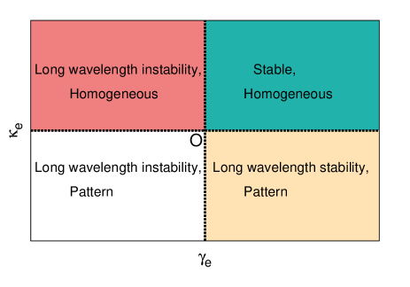
Figure 4: (Color online) Schematic phase diagram in $\gamma_{e}-\kappa_{e}$ plane. Symbol $O$ marks the origin $(0,0)$. Four distinct macroscopic behaviors are possible : (i) $\gamma_{e},\kappa_{e}>0$ (Stable, homogeneous), $\gamma_{e}>0,\kappa_{e}<0$ (long wavelength stability with patterns at $O(q^{2})$, (iii) $\gamma_{e}<0,\kappa_{e}>0$ (long wavelength unstable with no pattern) and (iv) $\gamma_{e},\kappa_{e}<0$ (long wavelength instability with patterns at $O(q^{2})$); see text.

III.2 Slow switching regime

We now briefly discuss the limit of slow switching regime, $\tau_{c}\gg\tau_{\phi}$. In order to extract the physics in this regime most effectively, we consider the limiting case and set $D_{c}=0$, in Eq. (2), so that $\tau_{c}\rightarrow\infty,\,\tau_{\times}\rightarrow 0$. Notice that in our model, even with $D_{c}=0$, the concentration dynamics does not freeze; this is essentially due to its coupling with the gradient of $\phi$ via the $\lambda_{2}$-term in Eq. (2). Then, assuming time dependences for $\phi$ and $\delta c\sim\exp(\tilde{\Lambda}t)$, we find

$$\tilde{\Lambda}\approx\frac{1}{2}\left[-q^{2}\kappa\pm 2q\sqrt{-\tilde{\Omega}_{1}\lambda_{2}}\right]$$ (25)

Hence, depending upon the sign of $\lambda_{2}$ (with $\tilde{\Omega}_{1}>0$), the system may exhibit either damping along with underdamped waves ($\lambda_{2}>0$) with speed $v_{0}=\sqrt{\tilde{\Omega}_{1}\lambda_{2}}$, or long-wavelength instability ($\lambda_{2}<0$) peruani ; remark_1 . In the linearly stable region, we find in the linearized theory, $\Delta\sim(\tilde{\Omega}_{1}^{2}D_{1}+Dv_{0}^{2})(\ln L)/\kappa$, yielding QLRO. This corresponds to $C_{s}(r)$ decreasing as $1/r^{\psi},\,\psi=(\tilde{\Omega}_{1}^{2}D_{1}+D\tilde{\Omega}_{1}\lambda_{2})/\kappa$. This is unaffected by the leading order nonlinearities. For $\lambda_{2}<0$, similar to the discussions above, a persistence length $\xi_{2}$ may be defined as $\xi_{2}=\kappa/\sqrt{\tilde{\Omega}_{1}|\lambda_{2}|}$ such that for system size $L>\xi_{2}$, $\Delta$ diverges, implying SRO. Lastly, coupling $\lambda$ remains irrelevant throughout (in a scaling sense) in all the cases discussed above. A phase diagram in the $\tilde{\Omega}_{1}-\lambda_{2}$ plane is given in Fig. 5, showing the linearly stable and unstable regions.

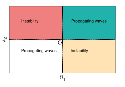
Figure 5: (Color online) Schematic phase diagram in $(\tilde{\Omega}_{1},\lambda_{2})$ plane in the linearized theory with $D_{c}\rightarrow 0$. Symbol $O$ marks the origin $(0,0)$. Two distinct macroscopic behaviors are possible : (i) $\tilde{\Omega}_{1},\lambda_{2}>0,\tilde{\Omega}_{1},\lambda_{2}<0$ : Propagating waves, and (ii) $\tilde{\Omega}_{1}>0,\lambda_{2}<0$ and $\tilde{\Omega}_{1}<0,\lambda_{2}>0$ : Instability in the system. see text. For the convenience of the reader, negative values of $\tilde{\Omega}_{1}$ have also been shown.

III.3 System behavior with autonomous mobility

Our results for both the fast and slow switching regimes crucially depend on the coupling $\lambda_{2}$; indeed, $\gamma=0$ if $\lambda_{2}=0$. In the agent-based models of Ref. frasca ; peruani ; pagona , agent mobility is fully autonomous, unaffected by the local phase, and hence these models imply $\lambda_{2}=0$ in the continuum. Nevertheless, even for those models it has been observed that for a sufficiently large $D_{c}$, oscillators tend to synchronize in systems of finite size. We now discuss this effect heuristically in a coarse-grained description. In these agent based models, while mobility is autonomous, phase fluctuations are still affected by diffusion. This happens essentially due to the particle diffusion enabling a test particle to have a larger number of contacts in its locality than without diffusion. This should renormalize the elastic modulus $\kappa$ that should now become a local quantity $\kappa(c)$ depending upon the local concentration fluctuation $\delta c$. Thus, in the coarse-grained hydrodynamic limit, expanding for small $\delta c$, we can phenomenologically replace $\kappa$ in Eq. (1) by

$$\kappa(c)=\kappa_{0}+\tilde{g}\delta c+g(\delta c)^{2},$$ (26)

where $\tilde{g}$ and $g$ are coupling constants. Averaging over $\delta c$-fluctuations yields an effecting spin stiffness $\kappa_{e}$ given by

$$\kappa_{e}=\kappa_{0}+g\langle(\delta c)^{2}\rangle.$$ (27)

For a given short range interaction, in a coarse-grained picture coupling $g$ should scale with the number of interactions $n_{0}$ in a unit time. Since $n_{0}$ should rise with $D_{c}$, $g$ should also rise with $D_{c}$. Thus, for a large enough $D_{c}$, $\kappa_{e}\gg(\ll)\kappa_{0}$ for $g>(<)0$. Clearly, with $g>0$ $\phi$-fluctuations are significantly suppressed for a large enough $D_{c}$, such that in a finite system the oscillators appear synchronized.

IV Summary and outlook

To summarize, we have constructed the dynamical equations for active hydrodynamics of a collection of nearly phase-coherent diffusively moving oscillators. Depending upon the details of the active processes, the system can display a wide-ranging nature of order, e.g., LRO, NLO and SRO. In particular, a large mobility can facilitate LRO for appropriate choices of the other model parameters. These are robust features, unaffected by an advecting velocity field. Our theory is generic, and is applicable to any nearly phase-ordered system of diffusively moving oscillators. We generally predict that the degree of synchronization and the nature of order in a 2d collection of mobile oscillators can be controlled by the underlying microscopic active processes. In the equilibrium limit, a collection of oscillators can only display QLRO at low $T$ classicalxy , and hence can be only partially synchronized. Thus LRO, NLO and SRO in this model are entirely of active origin. For an isolated, free standing system, $-\zeta v_{\alpha}$ in Eq. (5) should be replaced by $\eta\nabla^{2}v_{\alpha}$, $\eta$ being the fluid viscosity. The system does not show any new qualitative form of order in this limit. Oscillatory chemical reactions, oriented chiral live cytoskeletal extracts, in-vivo vertebrate segmentation clocks can thus be in a phase coherent or decoherent state, depending upon the details of the underlying active processes; the feedback of phase fluctuations on the mobility is expected to play an important role in the ensuing large scale behavior. Independent of the precise numerical values of model parameters, the general structure of the phase diagrams are robustly testable in related chemical and biologically inspired systems toiya1 ; toiya2 ; frank-exp . In experiments on in-vitro chiral cytoskeletal suspensions, $D_{c}$ may be controlled by changing the viscosity of the solvent; active parameters $\tilde{\Omega}_{1},\lambda_{2},\tilde{\Omega}_{3},\lambda_{1}$ may be controlled by changing $c_{0}$; the sign of $\gamma$ may be controlled by appropriate choices of contractile or extensile activties active-fluid . Numerical simulations of models for vertebrate segmentation clocks can be used to verify our results num-vertebrate . Our theory may be extended to account for superdiffusion markus with Lévy noises levy . Additional features, e.g., coupling delays and phase shifts frank2 , may be easily incorporated in our model. Large-scale numerical studies will ultimately be needed to go beyond the perturbative analysis presented here, and to study the role of topological defects that are neglected above. Our work should inspire new studies on agent-based models of synchronization in dynamical networks that would generalize the existing studies with autonomous particle mobility frasca ; pagona ; peruani ; net1 ; affect . We look forward to future attempts to verify our results in controlled experimental set ups. It would also be of interest to include large-scale systematic motion of the oscillators, controlled by external drive, in our model, and investigate how that may affect the nature of ordering elucidated here. We have effectively considered point particles without inter-particle interactions or any excluded volume interactions. Generalization of our model to groups of oscillators with distinct chiralities remains an interesting issue. Our model may be extended to include these features in straight forward ways. The insight gathered in this work should help design specific synchronization strategies in in-vivo systems with artificial microscopic agents. We expect our work to be a significant stepping stone in developing a general theory for active hydrodynamics of synchronization phenomena.

V Acknowledgement

The authors thank the Alexander von Humboldt Stiftung, Germany for partial financial support through the Research Group Linkage Programme (2016).

Appendix A Connection with CGLE

The complex Ginzburg Landau equation (CGLE) describes the coupled dynamics of the amplitude and phase of a complex field $Z=Z_{0}({\bf x},t)\exp[i\phi({\bf x},t)]$, where the amplitude $Z_{0}$ and phase $\phi$ are real functions of $\bf x$ and $t$.

$$\partial_{t}Z=-\frac{\delta{\mathcal{F}}}{\delta Z^{*}}-i\Gamma_{I}\frac{\delta{\mathcal{F}}}{\delta Z^{*}}+\Theta,$$ (28)

where $\Gamma_{I}$ is real,

$${\mathcal{F}}=\int d^{d}x[\frac{\tilde{r}}{2}|Z|^{2}+\frac{g}{2}|{\boldsymbol{\nabla}}Z|^{2}+u|Z|^{4}],$$ (29)

$\tilde{r}=0$ gives the mean field second order transition temperature, $u>0$. Here, $\Theta$ is a complex Gaussian noise with zero mean and a variance

$$\langle\Theta({\bf x},t)\Theta^{*}(0,0)\rangle=2D_{\xi}\delta({\bf x})\delta(t),\,\langle\Theta({\bf x},t)\Theta(0,0)\rangle=0.$$ (30)

If we now set $Z_{0}=1$, i.e., fixed amplitude for the complex field, $\phi$ then follows the real equation

$$\frac{\partial\phi}{\partial t}=g\nabla^{2}\phi+\Gamma_{I}[-\tilde{r}-2u+g({\boldsymbol{\nabla}}\phi)^{2}]+\tilde{\theta}.$$ (31)

Thus, Eq. (1) may be obtained by considering $\Gamma_{I}$ as a function of $c$ and with the identification $\kappa=g,\tilde{\Omega}_{0}=-\Gamma_{I}(r+2u),\lambda=-2\Gamma_{I}g,\tilde{\theta}=-\Re\Theta\sin\phi+\Im\Theta\cos\phi$. Here, $\Re$ and $\Im$ are, respectively, the real and imaginary parts of a complex number. This yields $\langle\tilde{\theta}({\bf x},t)\tilde{\theta}(0,0)\rangle=2D_{\xi}\delta({\bf x})\delta(t)$. We further equate $D_{\xi}$ with $D$ to recover the noise in Eq. (1) above; advection by a velocity $\bf v$ may be included straightforwardly above in Eq. (28), yielding the advective nonlinearity in Eq. (1) above. Similar density-dependent CGLE has been derived in different contexts recently erwin-cgle .

Appendix B Corrections to $\gamma$ for $L\gg L_{c}$ (without advective nonlinearities)

As shown in the main text,

$$\gamma_{e}=\gamma+\overline{\gamma}=\gamma+\frac{3\tilde{\Omega}_{3}\langle(\delta c)^{2}\rangle\lambda_{2}}{D_{c}}.$$ (32)

In the regime $\tau_{c}/\tau_{\times}\rightarrow 0$, for $L\gg L_{c}$,

$$\langle\delta c^{2}\rangle\approx\frac{\lambda_{2}^{2}D_{1}\tilde{\Omega}_{1}^{2}}{2\pi D_{c}^{4}\gamma}\ln L.$$ (33)

Hence,

$$\overline{\gamma}=3\frac{\lambda_{2}\tilde{\Omega}_{3}}{D_{c}}\langle(\delta c)^{2}\rangle\approx\Gamma\ln L,$$ (34)

which diverges logarithmically with $L$.

Appendix C Additional corrections to $\gamma>0$ and $\kappa$ from the advective nonlinearities ($\zeta>0$)

We work in the regime $\tau_{c}/\tau_{\times}\rightarrow 0$. Using Eq. (5), we substitute for $v_{\alpha}$ in Eq. (1) to obtain a term on the rhs of the latter

$$\frac{\lambda_{1}\alpha_{0}}{\zeta}\left[P_{\alpha\beta}\frac{\partial}{\partial x_{\gamma}}\left(\frac{\partial\phi}{\partial x_{\gamma}}\frac{\partial\phi}{\partial x_{\beta}}\right)\right]\frac{\partial\phi}{\partial x_{\alpha}}.$$ (35)

This yields a correction to $\kappa$, given by

$$\kappa^{\prime}=\frac{\lambda_{1}\alpha_{0}}{\zeta}\int\frac{d^{2}q}{(2\pi)^{2}}\frac{d\Omega}{2\pi}q^{2}\langle|\phi({\bf q},\Omega|^{2}\rangle.$$ (36)

The correction term is clearly finite for both $L<L_{c}$ and $L>L_{c}$. For $\lambda_{1}\alpha_{0}>0$, the correction to $\kappa$ (as well as $\kappa_{e}$) is positive and no qualitative change is introduced by advection at $O(q^{2})$. On the other hand, for sufficiently large negative $\lambda_{1}\alpha_{0}$, the effective $\kappa=\kappa_{e}+\kappa^{\prime}<0$ and the system becomes unstable at $O(q^{2})$, leading to formation of patterns in the eventual steady states.

We now substitute for $v_{\alpha}$ in Eq. (2) and then substitute for $\delta c$ in Eq. (1). We thus obtain a contribution on the rhs of Eq. (1) :

$$\frac{\tilde{\Omega}_{1}\lambda_{1}\alpha_{0}\lambda_{2}}{\zeta D_{c}^{2}\nabla^{2}}\left[P_{\alpha\beta}\frac{\partial}{\partial x_{\gamma}}\left(\frac{\partial\phi}{\partial x_{\gamma}}\frac{\partial\phi}{\partial x_{\beta}}\right)\right]\frac{\partial\phi}{\partial x_{\alpha}}.$$ (37)

This then yields another correction to $\gamma$, given by

$$\gamma^{\prime}=-\frac{\lambda_{1}\lambda_{2}\tilde{\Omega}_{1}\alpha_{0}}{\zeta D_{c}^{2}}\int\frac{d^{2}q}{(2\pi)^{2}}\frac{d\Omega}{2\pi}q^{2}\langle|\phi({\bf q},\Omega)|^{2}\rangle.$$ (38)

The correction to $\gamma$ is clearly finite for both $L>L_{c}$ and $L<L_{c}$. Thus, for $\lambda_{1}\lambda_{2}\tilde{\Omega}_{1}\alpha_{0}<0$, there are no qualitative changes introduced by advection at $O(q^{0})$. On the other hand for sufficiently large $\lambda_{1}\lambda_{2}\tilde{\Omega}_{1}\alpha_{0}>0$, the effective active damping can become negative, yielding instabilities at $O(q^{0})$. So far we assumed $\gamma>0$ (linear stability). In the linearly unstable case ($\gamma<0$), it is possible to suppress the linear instability for sufficiently large negative $\lambda_{1}\lambda_{2}\tilde{\Omega}_{1}\alpha_{0}<0$, such that effective active damping can become positive.

References

- (1) Synchronization A universal concept in nonlinear sciences by A. Pikovsky, M. Rosenblum and J. Kurths (Cambridge, 2001).
- (2) Sync: The emerging science of spontaneous order by S. Strogatz, Penguin (London, 2004).
- (3) J. Stricker et al, Nature (London) 456, 516 (2008).
- (4) T. Danino et al, Nature (London) 463, 326 (2010).
- (5) A. Prindle et al, Nature (London) 481, 39 (2012).
- (6) A. Prindle et al, Nature (London) 508, 387 (2014).
- (7) K. Uriu, L. G. Morelli and A. C. Oates, Semin. Cell Dev. 35, 66 (2014).
- (8) J. Buck and E. Buck, Nature 211, 562 (1966); J. Buck and E. Buck, Science, 159, 1319 (1968).
- (9) M. Rubenstein, A. Cornejo and R. Nagpal, Science 345, 795 (2014); M. Mijalkov et al, Phys. Rev. X 6, 011008 (2016).
- (10) B. Novák and J. J. Tyson, Nat. Rev. Mol. Cell. Biol. 9, 981 (2008).
- (11) See, e.g., I. H. Riedel-Kruse, C. Müller and A. C. Oates, Science 317, 1911 (2007); L. Herrgen et al, Curr. Biol. 20, 1244, (2010); D. J. Jörg et al, New J. Phys. 17, 093402 (2015).
- (12) P. Sevcik and I. Adamcikova, J. Chem. Phys. 91, 1012 (1989); P. Rouff, J. Phys. Chem. 97, 6405 (1993).
- (13) Nonlinear dynamics and Chaos by S. Strogatz, Levant Books (Calcutta, 2007).
- (14) K. Miyakawa and H. Isikawa, Phys. Rev. E, 65, 056206 (2002).
- (15) M. Toiya et. al. J. Phys. Chem. Lett., 1, 1241 (2010).
- (16) M. Toiya, V. K. Vanag and I. R. Epstein, Angew. Chem. Int. Ed., 47 7753 (2008).
- (17) H. Fukuda, H. Nagano and S. Kai, J. Phys. Soc. Jpn., 72 3 (2003).
- (18) I. Z. Kiss, Y. Zhai and J. L. Hudson, Phys. Rev. Lett., 88, 238301 (2002).
- (19) G. Migliorini, J. Phys. A: Math. Theor., 41, 324021 (2008).
- (20) S. H. Strogatz et. al., Physica D, 36, 23 (1989).
- (21) M. S. Paoletti, C. R. Nugent, and T. H. Solomon, Phys. Rev. Lett. 96, 124101 (2006).
- (22) T. Danino, O. Mondragón-Palomino, L. Tsimring, and J. Hasty, Nature (London) 463, 326 (2010).
- (23) F. Jülicher and J. Prost, Phys. Rev. Lett. 78, 4510 (1997).
- (24) S. Fürthauer, M. Strempel, S. W. Grill and F. Jülicher, Eur. Phys. J. E 35, 89 (2012);S. Fürthauer, M. Strempel, S. W. Grill and F. Jülicher, Phys. Rev. Lett. 110, 048103 (2013).
- (25) S. Fürthauer and S. Ramaswamy, Phys. Rev. Lett. 111, 238102 (2013).
- (26) M. Leoni and T. B. Liverpool, Phys. Rev. Lett. 112, 148104 (2014).
- (27) S. R. Naganathan, S. Fürthauer, M. Nishikawa, F.Jülicher and S. W. Grill, eLife 2014 3, e04165 (2014).
- (28) Y.-J. Jiang, B. L. Aerne, L. Smithers, C. Haddon, D. Ish-Horowicz, and J. Lewis, Nature (London) 408, 475 (2000).
- (29) A. C. Oates, L. G. Morelli, and S. Ares, Development 139, 625 (2012).
- (30) T. Gregor, K. Fujimoto, N. Masaki, and S. Sawai, Science 328, 1021 (2010).
- (31) A. Laskar, R. Singh, S. Ghose, G. Jayaraman, P. B. S. Kumar and R. Adhikari, Sci. Rep. 3, 1964 (2013).
- (32) F. Dörfler and F. Bullo, Automatica 50, 1539 (2014).
- (33) C. Li and G. Chen, Physica A 343, 263 (2004); J. Gómez-Gardeñes, Y. Moreno and A. Arenas, Phys. Rev. Lett. 98, 034101 (2007); F. Dörfler, M. Chertkov and M. Bullo, Proc. Nat. Sc. Acad (USA) 110, 2005 (2013).
- (34) M. Frasca et al, Phys. Rev. Lett. 100, 044102 (2008).
- (35) D. Levis, I. Pagonabarraga, and A. Díaz-Guilera, Phys. Rev. X 7, 011028 (2017).
- (36) R. Lauter, C. Brendel, S.J.M Habraken and F. Marquardt Phys. Rev. E 92, 012902 (2015).
- (37) D. J. Jörg, L. G. Morelli, S. Ares, and F. Jülicher, Phys. Rev. Lett. 112, 174101 (2014).
- (38) A. Buscarino, L. Fortuna and M. Frasca, Chaos 16, 015116 (2006).
- (39) F. Peruani, E. M. Nicola and L. G. Morelli, New J. Phys. 12, 093029 (2010).
- (40) K. Uriu, Y. Morishita and Y. Iwasa, Proc. Nat. Acad. Sc. (USA) 107, 4979 (2010).
- (41) K. Uriu and L. G. Morelli, Biophys. J. 107, 514 (2014).
- (42) P. C. Martin, O. Parodi, and P. S. Pershan, Phys. Rev. A 6, 2401 (1972).
- (43) S. Ramaswamy, Annu. Rev. Condens. Matter Phys. 1, 323 (2010); J.-F. Joanny, J. Prost, in Biological Physics, Poincare Seminar 2009, edited by B. Duplantier, V. Rivasseau (Springer, 2009) pp. 1-32; M. C. Marchetti, J. F. Joanny, S. Ramaswamy, T. B. Liverpool, J. Prost, M. Rao, and R. A. Simha Rev. Mod. Phys. 85, 1143 (2013).
- (44) Some model studies have considered the influence of the phase fluctuations on the oscillator movement; see, e.g., J. Ito and K. Kaneko, Phys. Rev. Lett. 88, 028701 (2001); T. Shibata and K. Kaneka, Physica D 181, 197 (2003); D. Tanaka, Phys. Rev. Lett. 99, 134103 (2007); T. Gross and B. Blasius, J. R. Soc. Interface 5, 259 (2008). Generalizing the existing studies, we consider the mutual effects of both phase fluctuations on the mobility and vice versa.
- (45) R. Grossmann, F. Peruani and M. Bär, Phys. Rev. E 93, 040102(R) (2016).
- (46) M. Porfiri, D. J. Stilwell, E. M. Bollt, and J. D. Skufca, Physica D 224, 102 (2006); J. D. Skufca and E. M. Bollt, Math. Biosci. Eng. 1, 347 (2004); N. Fujiwara, J. Kurths, and A. Diaz-Guilera, Phys. Rev. E 83, 025101 (2011); S. Sarkar and P. Paramanand, Chaos 20, 043108 (2010); J. Gomez-Gardenes, V. Nicosia, R. Sinatra, and V. Latora, Phys. Rev. E 87, 032814 (2013).
- (47) R. Kapral and K. Showalter, Chemical Waves and Patterns Kluwer, Dordrecht, 1995.
- (48) T. S. Briggs and W. C. Rauscher, J. Chem. Educ. 50, 496 (1973).
- (49) W. C. Bray, J. Am. Chem. Soc. 43, 1262 (1921).
- (50) H. Landolt, Ber. Dtsch. Chem. Ges. 19, 1317 (1986).
- (51) P. M. Chaikin and T. C. Lubensky, Principles of condensed matter physics (Cambridge University Press, Cambridge 2000).
- (52) T. Banerjee, N. Sarkar and A. Basu, Phys. Rev. E, 92, 062133 (2015).
- (53) This was originally introduced to describe the depression of the order parameter from its zero temperature maximum due to the thermal fluctuations in the ordered phases; see, e.g., Ref. classicalxy .
- (54) See, e.g., T. C. Adhyapak, S. Ramaswamy, J. Toner, Phys. Rev. Lett. 110, 118102 (2013); L. Chen and J. Toner, Phys. Rev. Lett. 111, 088701 (2013).
- (55) Y. Kuramoto, Chemical Oscillations, Waves, and Turbulence, Springer Series in Synergetics (Springer, Berlin, 1984). see also D. J. Jorg, arXiv: 1501:05815.
- (56) See J. Denk et al, Phys. Rev. Lett. 116, 178301 (2016) for a study in CGLE with density-dependent coefficients as a model for active curved polymers on membranes.
- (57) E. Altman, L.M. Sieberer, L. Chen, S. Diehl and J. Toner, Phys. Rev. X 5, 011017 (2015).
- (58) M. Kardar, G. Parisi and Y-C. Zhang, Phys. Rev, Lett., 56, 889 (1986).
- (59) The form of the additive noise in Eq. (2) ensures that concentration follows a conserved dynamics. Alternatively, one may keep only the deterministic terms in the current and then is the noise in Eq. (2); has the correlation . This leaves our results on correlations or unchanged.
- (60) Darcy, Les fontaines publiques de la ville de Dijon, Paris: Dalmont (1856); see also S. Whitaker, Transport in Porous Media 1, 3 (1986).
- (61) See, e.g., R. Ruiz and D. R. Nelson, Phys. Rev. A 23, 3224 (1981).
- (62) We ignore a similar symmetry-allowed -dependent feedback term in (5) for simplicity.
- (63) Y. Kuramoto, Chemical Oscillations, Waves, and Turbulence (Springer Science & Business Media, New York, 2012), Vol. 19.
- (64) J. A. Acebrón, L. L. Bonilla, C. J. Perez-Vicente, F. Ritort, and R. Spigler, Rev. Mod. Phys. 77, 137 (2005).
- (65) P.-G. de Gennes, J. Prost, The Physics of Liquid Crystals (Clarendon, Oxford, 1993).
- (66) R. Voituriez, J. F. Joanny and J. Prost, Europhys. Lett.
- (67) A. Basu, J.-F. Joanny, F. Jülicher and J. Prost, New J. Phys. 14, 115001 (2012).
- (68) R. A. Simha and S. Ramaswamy, Phys. Rev. Lett. 89, 058101 (2002); J. Toner, Y. Tu and S. Ramaswamy, Annals of Phys. 318, 170 (2005).
- (69) The sign of , in conjunction with the signs of other model parameters control whether the active contribution to favors or opposes the diffusive current . For instance, with the choice (as made through out this text), implies that the local nonuniformity in the phase of the oscillators decreases (increases) as the local nonuniformity in the concentration of the moving oscillators rises (decreases). For example, in a live cell cytoskeletal extract, would imply that an increasing concentration of the moving oscillators can destabilize the phase coherence.
- (70) We assume a finite . For small and large , with a finite .
- (71) S. Assenza et al, Sc. Rep. 1, 99 (2011).
- (72) Since we are interested in the long-wavelength limit, terms have been neglected in comparison to and .
- (73) K. Uriu, Y. Morishita and Y. Iwasa, Proc. Natl. Acad. Sci. USA 107, 4979 (2010).
- (74) R. Klages, G. Radons, and I. M. Sokolov, Anomalous Transport: Foundations and Applications (Wiley, Hoboken, NJ, 2008).