Non-equilibrium variational cluster perturbation theory:
quench dynamics of the quantum Ising model

Abstract

We introduce a variational implementation of cluster perturbation theory (CPT) to address the dynamics of spin systems driven out of equilibrium. We benchmark the method with the quantum Ising model subject to a sudden quench of the transverse magnetic field across the transition or within a phase. We treat both the one-dimensional case, for which an exact solution is available, as well the two-dimensional one, for which has to resort to numerical results. Comparison with exact results shows that the approach provides a quite accurate description of the real-time dynamics up to a characteristic time scale $\tau$ that increses with the size of the cluster used for CPT. In addition, and not surprisingly $\tau$ is small for quenches across the equilibrium phase transition, but can be quite larger for quenches within the ordered or disordered phases.

I Introduction

The remarkable progresses of experiments on ultracold atoms trapped in optical latticesBloch ; Lewenstein ; Strohmaier have boosted a great interest in the nonequilibrium dynamics of closed quantum systems, especially when they are suddenly pushed across a quantum critical pointSachdev ; Suzuki . A rich theoretical activity thus flourished, starting from the paradigmatic example of quantum criticality, namely the quantum Ising model.Meinert ; Rossini ; Calabrese

Developing suitable tools for handling many-body systems out of equilibrium is a big challenge that started some time ago with the pioneering works by Kubo Kubo , Schwinger Schwinger , Kadanoff and Baym Kadanoff , and Keldysh Keldysh . This effort continued with the work by WagnerWagner , who unified the Feynman, Matsubara, and Keldysh perturbation theories into a single and very flexible formalism, till latest developments related to dynamical mean field and related cluster-embedding methods (see, e.g. Freericks ; Schmidt ; Hofmann ; Jung ; Knap3 ; Aoki ; Balzer1 ; Balzer2 ; Gramsch ; ar.kn.13 ; do.nu.14 ; do.ga.15 ). We shall in particular be concerned with the very recent out-of-equilibrium generalization of cluster perturbation theory (CPT) Senechal ; Gros , which is attractive and conceptually simple Balzer2 . In CPT the lattice is divided into small clusters which can be diagonalized exactly. The inter-cluster terms are then treated within strong-coupling perturbation theory. Its nonequilibrium version allows to investigate the unitary quantum evolution in the thermodynamic limit, accounting for non-local correlations on a length scale defined by the size of the considered cluster. Besides the simplicity of the formulation, the efficiency and accuracy of the specific implementation is also of major importance.

The main purpose of this work is to develop a non-equilibrium variational implementation of CPT for spin systems. We test the method on the quantum Ising model after a sudden quench of the transverse field. Since the model is exactly solvable in one dimension we have the possibility to benchmark the approach. We also investigate the same model in two dimensions where an exact solution is not available. In this case, we compare with finite-size exact diagonalization results. We discuss in detail how to efficiently implement the method so to allow reaching relatively long simulation times with moderate computational effort.

The paper is organised as follows. In section II the non-equilibrium Green’s function formalism is briefly presented. The model we shall study is introduced in section III. Section IV describes the CPT method together with its self-consistent variational improvement. Results are reported in Sec. V. Section VI is devoted to concluding remarks.

II Non-Equilibrium Green’s functions

In this section we briefly outline the non-equilibrium Green’s function formalism to set up the notations that we shall use throughout the paper. There is a wide literature on the subject but in this work we mainly follow the Kadanoff-Baym-Wagner scheme Kadanoff ; Wagner .

Consider a system initially (at time $t_{0}=0$) at equilibrium described by a Hamiltonian $H_{eq}$ and temperature $1/\beta$. At $t>t_{0}$ a generic time dependent Hamiltonian $H(t)$ is switched on. The non-equilibrium formalism works through averages of time-ordered products of operators along the Kadanoff-Baym contourKadanoff ; Keldysh ; Danielewicz ; Rammer shown in Fig. 1. The contour is composed of three branches: it starts at $t_{0}=0$, runs up to $t_{max}$ and then back to the initial time, and finally moves parallel to the imaginary axis up to $\tau=-i\beta$.

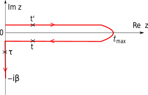
Figure 1: The $L$ shaped Kadanoff-Baym contour ${\cal C}$ . The arrows indicate the contour ordering. For example, $t^{\prime}$ lies ahead of $t$ in the ordering ($t>t^{\prime}$), i.e., operators at $t^{\prime}$ are sorted to the right by the contour ordering

Due to the lack of time translation invariance, the non-equilibrium single-particle Green’s function depends on two time variables rather than on their difference and is defined as the contour ordered expectation value

$$\begin{split}G_{i,j}&(z,z^{\prime})=-i\langle{\cal T}_{\cal C}a_{i}(z)a_{j}^{\dagger}(z^{\prime})\rangle=\\ &=-i\theta^{\cal C}(z-z^{\prime})\langle a_{i}(z)a_{j}^{\dagger}(z^{\prime})\rangle-i\theta^{\cal C}(z^{\prime}-z)\langle a_{j}^{\dagger}(z^{\prime})a_{i}(z)\rangle\,,\end{split}$$ (1)

where $a_{i}^{\dagger}(a_{i})$ are the creation (annihilation) operators for particles, in the present case bosons, at site $i$ and $z,z^{\prime}$ are variables on the contour ${\cal C}$, and can be real or imaginary depending on the branch of the contour in which they lay. The time evolution of the operators on the Kadanoff-baym contour is defined in the Heisenberg picture with Hamiltonian $H(z)$. ${\cal T}$ is the time ordering operator and is defined via the contour step function $\theta^{\cal C}(z-z^{\prime})$. The averages in Eq. (1) are over the initial equilibrium Hamiltonian $H_{eq}$ at temperature $1/\beta$.

The Dyson equation reads

$$\hat{G}=\hat{G_{0}}+\hat{G_{0}}\bullet\hat{\Sigma}\bullet\hat{G}\,,$$ (2)

where $\hat{G_{0}}$ is the bare Green’s function and $\hat{\Sigma}$ the self-energy. The product symbol $\bullet$ denotes the matrix multiplication in space and the integration over the time variables along the contour ${\cal C}$.

For a given Green’s function $\hat{G}(z,z^{\prime})$ each variable $z,z^{\prime}$ can lay on one of the three branches of the contour in Fig. 1. This prompts an alternative representation of $\hat{G}$ as a $3\times 3$ matrix, as introduced by Wagner Wagner . Of the $9$ matrix elements, only $6$ are linearly independent, so that after a suitable transformation one is left with $6$ nonzero terms, which are referred to as the retarded $(G^{R})$, advanced $(G^{A})$, Keldysh $(G^{K})$, left-mixing $(G^{\rceil})$, right-mixing $(G^{\lceil})$ and Matsubara Green’s function $(G^{M})$. They are explicitly given as

$$\begin{split}G_{i,j}^{R}(t,t^{\prime})=-i\theta(t-t^{\prime})\langle[a_{i}(t),a_{j}^{\dagger}(t^{\prime})]\rangle\,,\\ G_{i,j}^{A}(t,t^{\prime})=G_{j,i}^{R}(t^{\prime},t)^{*}\,,\\ G_{i,j}^{K}(t,t^{\prime})=-i\langle\{a_{i}(t),a_{j}^{\dagger}(t^{\prime})\}\rangle\,,\\ G_{i,j}^{\rceil}(t,\tau)=-i\langle a_{j}^{\dagger}(\tau)a_{i}(t)\rangle\,,\\ G_{i,j}^{\lceil}(\tau,t)=-i\langle a_{i}(\tau)a_{j}^{\dagger}(t)\rangle\,,\\ G_{i,j}^{M}(\tau,\tau^{\prime})=-\langle{\cal T}_{\tau}a_{i}(\tau)a_{j}(\tau^{\prime})\rangle\,,\end{split}$$ (3)

where $t$ and $t^{\prime}$ are real times and $\tau,\tau^{\prime}\in[0,-i\beta]$. In the above equations $\{\dots\}$ and $[\dots]$ stem for anticommutator and commutator, respectively.

III Hamiltonian

The Hamiltonian of the Ising model in a transverse field is given by

$$H=-J\sum_{\langle i,j\rangle}S_{i}^{x}S_{j}^{x}+h\sum_{i}S_{i}^{z}\,,$$ (4)

where $\langle i,j\rangle$ means summation over nearest neighbor spins, and $h$ is the strength of the magnetic field, with $J>0$ and $h>0$. In the following we shall work in units of $J=1$. The Hamiltonian of Eq. (4) in one dimension has an exact solution which is obtained by a Jordan-Wigner transformation that maps the system onto a quadratic Hamiltonian for spinless fermions, which can be exactly solved Lieb ; Pfeuty . On the other hand, in two dimensions an exact solution is not available Oleg .

Cluster embedded techniques such as CPT in equilibrium have been applied to fermionic and bosonic systemsPotthoff_vca1 ; Potthoff_vca2 ; Koller ; Aichhorn ; Zacher . Out of equilibrium, CPT has been applied to the fermionic Hubbard modelBalzer2 ; Gramsch . Here we formulate nonequilibrium CPT for spin systems, exploiting the well known equivalence between spin-1/2 operators are hard-core bosons. We also provide a variational improvement of it, which allows to treat the ordered phase.

Specifically, if we assume that spin-up corresponds to the presence of a hard-core boson, and spin-down to its absence, the following relationships between spin and boson operators holdSachdev

$$\begin{split}&S^{+}\rightarrow a^{\dagger}\,,\\ &S^{-}\rightarrow a\,,\\ &S^{z}\rightarrow a^{\dagger}a-1/2\,,\\ &S^{x}\rightarrow(a+a^{\dagger})/2\,,\end{split}$$ (5)

where $S^{+}$ and $S^{-}$ are raising and lowering spin operators, respectively.

The Hamiltonian in the bosonic representation then becomes

$$\begin{split}H=-\frac{J}{4}\sum_{\langle i,j\rangle}(a_{i}a_{j}+a_{i}^{\dagger}a_{j}^{\dagger}+a_{i}a_{j}^{\dagger}+a_{i}^{\dagger}a_{j})\\ +h\sum_{i}(a_{i}^{\dagger}a_{i}-1/2)+U\sum_{i}n_{i}(n_{i}-1)\end{split}$$ (6)

where the on-site Hubbard-like term enforces the hard-core constraint when $U\to\infty$, and $n_{i}=a^{\dagger}_{i}a_{i}$. Since the Hamiltonian contains both normal and anomalous hopping terms, Green’s functions with anomalous terms are needed to study the system (see appendix A).

IV Method

IV.1 Cluster perturbation theory

Cluster perturbation theory (CPT)Gros ; Senechal is a simple quantum cluster method to deal with correlated systems. In this approach the idea is to embed a finite cluster of sites, for which a numerically exact solution is affordable, into the infinite lattice. In practice the starting point is to partition the original $D$-dimensional lattice of linear size $L$ into clusters of linear size $L_{c}$ with open boundaries. Fig. 2 shows an example for a tiling in $D=1$ and $L_{c}=4$.

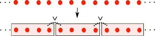
Figure 2: Partitioning of a D=1 lattice into clusters with size $L_{c}=4$. The inter-cluster hopping is denoted by $V$

All clusters are considered as supercells that form a superlattice, each supercell being identified by a superlattice vector $r$. The sites within each cluster are in turn labelled by vectors $R$. The lattice Hamiltonian $H$ is thus written as

$$H=H_{0}+V\,,$$ (7)

where $H_{0}$ corresponds to the cluster Hamiltonian and $V$ describes the inter-cluster terms. CPT Green’s function can be obtained by a subsequent expansion in powers of the inter-cluster hopping. Diagrammatic Metzner ; Pairlaut and cluster dual fermion approachesHafermann provide a systematic expansion in terms of the inter-cluster terms, which then has to be truncated at some order. Within strong-coupling perturbation theorySenechal ; Senechal2 one obtains an expression for the lattice Green’s function at lowest order

$$G(\omega)=G_{0}(\omega)-G_{0}(\omega)VG(\omega)\,,$$ (8)

where $V$ is the matrix representation of the inter-cluster hopping, $G_{0}(\omega)$ the exact equilibrium Green’s function of the cluster and the product is just a matrix multiplication in lattice sites. The Green’s function $G_{0}$ is diagonal in $r$ and identical for all supercells, whereas $V$ is off-diagonal in $r$. Because of superlattice translation invariance, the above equation is simpler in momentum space. After partial Fourier transform, $r\rightarrow q$, the CPT equation transforms into

$$G(q,\omega)=G_{0}(\omega)-G_{0}(\omega)V(q)G(q,\omega)\,,$$ (9)

where now $G$, $G_{0}$ and $V$ are matrices in the label $R$ of the sites within each supercell. The CPT is a conceptually simple method that nevertheless includes short-range correlations on the scale of cluster size and therefore requires moderate computational resources.

The idea of CPT can be straightforwardly transferred to non-equilibrium situation by replacing the equilibrium frequency-dependent Green’s functions with the contour ordered ones. The authors of Ref. Balzer2 have developed a non-equilibrium formulation for CPT (NE-CPT) and examined how the technique works for the Fermi-Hubbard model. The NE-CPT equation reads as following

$$\hat{G}(q)=\hat{G}_{0}+\hat{G_{0}}\bullet\hat{V}(q)\bullet\hat{G}(q)\,.$$ (10)

The solution of Eq. (10) provides the non-equilibrium CPT Green’s function $\hat{G}(q)$. In the NE-CPT equation the product symbol $\bullet$ denotes not only the matrix multiplication but also an integration over time variables along the contour $\cal{C}$. Furthermore $\hat{V}(q)=V(q)\bigotimes\mathbb{1}$ where $\mathbb{1}$ is a $\delta$-function on the contour, i.e., $\delta(z^{\prime}-z)=\mathbb{1}$. In what follows we shall omit the momentum dependence to simplify notations. The explicit integral form of Eq. (10) is

$$\hat{G}(z,z^{\prime})=\hat{G}_{0}(z,z^{\prime})+\int_{\cal{C}}dz_{1}\,\hat{G}_{0}(z,z_{1})V\hat{G}(z_{1},z^{\prime})\,,$$ (11)

where integration is carried out along the three branches of the contour $\cal{C}$ in Fig. 1, i.e.

$$\int_{\cal{C}}dz_{1}=\int_{0}^{t_{max}}dt-\int_{0}^{t_{max}}dt+\int_{0}^{-i\beta}d\tau\;.$$ (12)

The numerical solution of the generic contour equation (11) requires discretization of the time variable. A straightforward but not efficient solution for $\hat{G}$ involves a matrix inversionBalzer2 where large matrices in discretized time are used. In this manner reaching long time dynamics is computationally prohibitive. Alternatively, by using the Kadanoff-Baym equations Kadanoff ; Bonitz one can derive the same integral equation, Eq. (11, for the components of $\hat{G}$ in the Wagner representation (see Eq. (3)). A practical application of this approach to non-equilibrium dynamical mean-field theory (NE-DMFT) has been presented by TranTran . This method takes advantage of the causality of the integral equations: the properties of the system at specific time $t=t_{1}$ do not depend on the information at $t>t_{1}$ and so its a priori knowledge is not required in the calculation. Here we follow this approach but for spatially inhomogeneous systems. For details of the procedure and technical issues see Appendix (A)

IV.2 Variational cluster perturbation theory

Within CPT one is free to add an arbitrary single-particle term $-\Delta$ to the cluster Hamiltonian $H_{0}$ (Eq. (7)) provided that it is then subtracted perturbatively, i.e. added to $V$, such that the Hamiltonian $H$ remains unchanged. The CPT expansion is now carried out in the new perturbation $\bar{V}=V+\Delta$ with the new cluster Hamiltonian $H^{\prime}=H_{0}-\Delta$. While ideal exact results should not depend on $\Delta$, in practice results do depend on $\Delta$ due to the approximate nature of the CPT expansion.
In this work we shall consider a $Z_{2}$ symmetry breaking term

$$\Delta=\sum_{R=1}^{L_{c}}f_{R}\,S_{R}^{x}=\sum_{R=1}^{L_{c}}\frac{f_{R}}{2}\Big{(}a_{R}+a_{R}^{\dagger}\Big{)}\,,$$ (13)

where $f_{R}$ are real variational parameters to be fixed. We show below that accounting for this variational term is crucial to describe the ordered phase of quantum Ising model. The optimum value of the variational parameters $f_{R}$ should be determined through a variational principleHofmann ; Enrico ; Knap2 . Here we shall resort to a simplified version of the variational procedure introduced in  Enrico ; Knap2 . Specifically, we fix the variational parameters within a self-consistent approach where the inter-cluster term $S_{i}^{x}\,S_{j}^{x}$ is replaced with its mean-field approximation as

$$S_{i}^{x}S_{j}^{x}=\langle S_{i}^{x}\rangle S_{j}^{x}+S_{i}^{x}\langle S_{j}^{x}\rangle-\langle S_{i}^{x}\rangle\langle S_{j}^{x}\rangle\,.$$ (14)

In one dimension, for example, upon tiling the infinite lattice into clusters of size $L_{c}$, the mean-field expression for the supercell Hamiltonian at equilibrium is

$$H^{\prime} = -J\sum_{R=1}^{L_{c}-1}S_{R}^{x}S_{R+1}^{x}+h_{0}\sum_{R=1}^{L_{c}}S_{R}^{z}$$ (15)

$$-f_{L_{c}}\,S_{1}^{x}-f_{1}\,S_{L_{c}}^{x}\,,$$

where $f_{R}=J\langle S_{R}^{x}\rangle$, $R=1,L_{c}$ are the mean-field self-consistency conditions and, by translational symmetry, we shall set $f_{1}=f_{L_{c}}$.

Out of equilibrium the variational parameters become time dependent. The protocol we shall implement is a sudden quench of the magnetic field from $h_{0}$ to a different value $h$. Therefore the explicit time dependent mean-field cluster Hamiltonian becomes

$$H^{\prime}(t) = -J\sum_{R=1}^{L_{c}-1}S_{R}^{x}S_{R+1}^{x}+h\sum_{R=1}^{L_{c}}S_{R}^{z}$$ (16)

$$-f_{L_{c}}(t)\,S_{1}^{x}-f_{1}(t)\,S_{L_{c}}^{x}\,,$$

with the self-consistency condition

$$f_{R}(t)=f_{R}(t)^{*}=J\,\langle\Psi(t)|S_{R}^{x}|\Psi(t)\rangle\,,$$ (17)

where $|\Psi(t)\rangle$ is the time evolved cluster wavefunction. In order to evaluate the time dependent variational parameters $f_{R}(t)$ we expand the latter to linear order

$$|\Psi(t+\Delta t)\rangle\approx\Big{(}1-iH^{\prime}(t)\Delta t\Big{)}\,|\Psi(t)\rangle+\mathcal{O}(\Delta t^{2})$$ (18)

starting from the initial equilibrium state $|\Psi(t=t_{0})\rangle$. As a result, the parameters $f_{i}(t+\Delta t)$ can be taken as

$$f_{i}(t+\Delta t)\approx J\langle\Psi(t+\Delta t)|S_{i}^{x}|\Psi(t+\Delta t)\rangle$$ (19)

at each time step.

IV.3 CPT corrections to the order parameter

Due to the presence of anomalous terms linear in creation and annihilation operators the new perturbation $\bar{V}$ including $\Delta$ (Eq. 13) is not quadratic in the boson operators and therefore one has to generlaize CPT to deal with anomalous terms as well- The way to do this (see Ref. Knap2 ; Enrico ) is to first perform starndard CPT on top of the cluster Hamiltonian $H^{\prime}$ (Eq. 15) by using just the quadratic part of $V$ as a perturbation. The CPT correction to the condensate can be then obtained by using an expression derived within a so-called pseudoparticle formulation of CPT Knap2 for the Bose-Hubbard model in the superfluid phase, and, subsequently confirmed more formally within a self-energy functional approach. Knap2 For the equilibrium case, one obtains

$$G^{-1}\langle A\rangle=G^{{}^{\prime}-1}\langle A\rangle^{\prime}+F\,,$$ (20)

where $G$ and $\langle A\rangle$ are the CPT corrected Green’s function and expectation value of the condensate, respectively, while the terms with prime stands for their cluster values. The vector $F$ describes the variational parameters $f$ of Eq. (13). In Eq. (20) the Green’s functions are $2L_{c}\times 2L_{c}$ Nambu matrices and the $\langle A\rangle$, $\langle A\rangle^{\prime}$ and $F$ are $2L_{c}$ Nambu vectors, namely

$$\langle A\rangle^{\prime}=\begin{bmatrix}\langle a^{\prime}_{1}\rangle\\ .\\ .\\ .\\ \langle a^{\prime}_{L_{c}}\rangle\\ \langle a_{1}^{{}^{\prime}{\dagger}}\rangle\\ .\\ .\\ .\\ \langle a_{L_{c}}^{{}^{\prime}{\dagger}}\rangle\end{bmatrix}\;,\;\langle A\rangle=\begin{bmatrix}\langle a_{1}\rangle\\ .\\ .\\ .\\ \langle a_{L_{c}}\rangle\\ \langle a_{1}^{\dagger}\rangle\\ .\\ .\\ .\\ \langle a_{L_{c}}^{\dagger}\rangle\end{bmatrix}\;,\;2F=\begin{bmatrix}f_{1}\\ .\\ .\\ .\\ f_{L_{c}}\\ f_{1}^{*}\\ .\\ .\\ .\\ f_{L_{c}}^{*}\end{bmatrix}\,.$$ (21)

Out of equilibrium it is straightforward to generalize Eq. (20) to an equation along the contour:

$$\hat{G}^{-1}\bullet\hat{A}=\hat{G}^{{}^{\prime}-1}\bullet\hat{A}^{\prime}+\hat{F}\,,$$ (22)

where the ingredients are now contour functions. Again, the symbol $\bullet$ represents matrix multiplication in space and time integration along the contour. We further simplify this expression by multiplying both sides of it by $\hat{G}$ from the left. This leads to

$$\hat{A}=\hat{G}\bullet\hat{G}^{{}^{\prime}-1}\bullet\hat{A}^{\prime}+\hat{G}\bullet\hat{F}\,,$$ (23)

where we have used the fact that $\hat{G}\bullet\hat{G}^{-1}=\mathbb{1}$. Via the CPT equation (10) one can further derive the expression

$$\hat{G}\bullet\hat{G}^{{}^{\prime}-1}=\mathbb{1}+\hat{G}\bullet\hat{V}\,.$$ (24)

After substituting into Eq. (23), one finally gets the following equation for the condensate including CPT correction

$$\hat{A}=\hat{A}^{\prime}+\hat{G}\bullet\hat{V}\bullet\hat{A}^{\prime}+\hat{G}\bullet\hat{F}\,.$$ (25)

We rewrite this equation by expressing the contour integration explicitly as

$$\hat{A}(z)=\hat{A}^{\prime}(z)+\int_{c}d\bar{z}\,\hat{G}(z,\bar{z})\Big{(}V\hat{A}^{\prime}(\bar{z})+\hat{F}(\bar{z})\Big{)}\,,$$ (26)

where $z,\bar{z}$ are contour variables (see Fig. 1). By employing Langreth theorem Langreth one can break down the contour integrations into contributions on the real and imaginary time axes. For the condensate on the real time branch of the contour we get

$$\begin{split}A(t)=A^{\prime}(t)&+\int_{0}^{t}d\bar{t}\,G^{R}(t,\bar{t})\Big{(}VA^{\prime}(\bar{t})+F(\bar{t})\Big{)}\\ &+\int_{0}^{-i\beta}d\bar{\tau}\,G^{\rceil}(t,\bar{\tau})\Big{(}VA^{\prime}(\bar{\tau})+F(\bar{\tau})\Big{)}\,,\end{split}$$ (27)

where we have used $G^{R}(t,t^{\prime})=\theta(t,t^{\prime})\Big{(}G^{>}(t,t^{\prime})-G^{<}(t,t^{\prime})\Big{)}$. Similarly for the condensate on the Matsubara branch we derive

$$A(\tau)=A^{\prime}(\tau)+\int_{0}^{-i\beta}d\bar{\tau}\,G^{M}(\tau,\bar{\tau})\Big{(}VA^{\prime}(\bar{\tau})+F(\bar{\tau})\Big{)}\,.$$ (28)

We note from Eq. (27) that, in order to evaluate $A(t)$ within CPT, the mixing Green’s function $G^{\rceil}$ and retarded Green’s function $G^{R}$ have to be determined first. It is crucial to employ high-order numerical integration schemes to accurately simulate up to long times. We refer to Appendix. (A) for more details.

IV.4 Magnetization

The time dependent magnetization is obtained as

$$S^{z}(t)=\frac{1}{L}\sum_{q}\sum_{R=1}^{L_{c}}\,\big{\langle}\;a_{R,q}^{\dagger}(t)\,a_{R,q}(t)-\frac{1}{2}\;\big{\rangle}\,,$$ (29)

where $L=N_{c}L_{c}$ is the total size of the lattice. $\langle a_{R,q}^{\dagger}(t)\,a_{R,q}(t)\rangle$ can be extracted from the lesser component of the Green’s function within CPT

$$\langle a_{R,q}^{\dagger}(t)\,a_{R,q}(t)\rangle=i\,G_{RR,q}^{<}(t,t)\,.$$ (30)

Adding the contribution from the condensate, the final expression for the magnetization is

$$S^{z}(t) = \frac{1}{L}\sum_{q}\sum_{R}\,i\,G_{RR,q}^{<}(t,t)$$

$$+\frac{1}{L_{c}}\sum_{R=1}^{L_{c}}\,\bigg{(}\langle\,a_{R}^{\dagger}(t)\,\rangle\;\langle\,a_{R}(t)\,\rangle-\frac{1}{2}\bigg{)}\,,$$

where $\langle a_{R}^{\dagger}(t)\rangle$ and $\langle a_{R}(t)\rangle$ are elements of the vector $A(t)$, see Eq. (27).
For a finite lattice with open boundary conditions, translation symmetry is lost and therefore the magnetization is position dependent, more pronounced close to the boundaries.

V Results

In the following we apply the technique discussed in the previous section for both equilibrium and nonequilibrium situations. Moreover, by comparing the results with exact ones in one dimension we asses the accuracy of the method.

V.1 Equilibrium results

Before applying the technique out of equilibrium we investigate its ability to describe the system already in equilibrium. This is actually a necessary step since the present non-equilibrium protocol assumes that the system is prepared as the ground state of an initial Hamiltonian and is then evolved with a different Hamiltonian. Therefore, an accurate equilibrium state is a prerequisite for getting a sensible after-quench dynamics. The CPT method can work directly in the thermodynamic limit, however, in order to compare with exact results in one dimension, we shall consider a finite system with linear size $L=8$ with open boundary conditions. In the CPT method the procedure is thus to divide the system into two parts, $A$ and $B$, each one with size $L_{c}=4$, and then treat the inter-cluster term perturbatively, see Fig. 2.

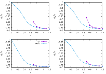
Figure 3: Magnetization along the $z$ direction versus magnetic field for different sites on a lattice of size $L=8$ with open boundary condition. Cluster size in CPT is $L_{c}=4$. Exact results are also being reported for comparison.

We first set the anomalous term to zero in the cluster Hamiltonian, i.e, $\Delta=0$ in Eq. (13). In Fig. 3 we display the magnetization parallel to the magnetic field, $\langle S^{z}\rangle$, for sites $i=1$ to $i=4$ compared with exact result. As we see CPT works well for large values of magnetic field and reproduces results close to exact ones. By contrast, upon decreasing $h$ the accuracy decreases. Standard CPT totally fails close to the mean-field critical field ($h_{c}=0.7$). Therefore the standard CPT is unable to correctly describe the physics for $h<0.7$.

This kind of instability is well known in approaches based on the bosonic Bogoliubov approximation, such as the spin-wave approximation. The Green’s function for free bosons ($U=0$ in the Hamiltonian of Eq. (6)) has two poles at $z=\pm\sqrt{h^{2}-\frac{J^{2}}{4}}$. It is clear that for $h<J/2$ the poles move to the imaginary axis, a clear signal of an instability.

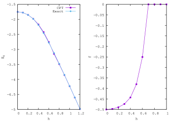
Figure 4: Left panel: Ground state energy from CPT compared with the exact value for lattice of size $L=8$ with open boundary condition. Right panel: $f=J\langle S_{1B}^{x}\rangle=J\langle S_{4A}^{x}\rangle$

The same explanation applies to the interacting Hamiltonian Eq. (6) and to the instability seen in Fig. 3. The poles of the Green’s function become complex for small values of magnetic field, i.e. for $h<0.7$. This is the region where the hard-core constraint of the bosons becomes important and the standard CPT fails to satisfy this condition. We control the location of the poles by adding the variational term $\Delta$ in Eq. (13) to the cluster Hamiltonian, which explicitly breaks the $Z_{2}$ symmetry and induces the spontaneous breaking of such symmetry at low fields. After finding self-consistently the optimum value for the variational parameters we compute the CPT corrections as explained in the previous section.

In Fig. 4 on the left panel we show the result for the ground state energy compared with the exact one. The agreement is quite good in the whole range of magnetic fields. On the other hand, it is well known that the energy is a quantity that is not much sensitive to perturbations, so one could argue that this agreement is not significative. On the other hand, the right panel shows the value of the variational parameter $f=J\langle S_{1B}^{x}\rangle=J\langle S_{4A}^{x}\rangle$. This quantity shows a phase transition at $h_{c}=0.7$, below which $\langle S^{x}\rangle$ acquires a finite value. Strictly speaking such a phase transition should not occur on a finite size system, where $\langle S^{x}\rangle$ must be zero by symmetry, so its emergence is a spurious results that derives from the variational scheme. In the thermodynamic limit the transition does instead occur, although the critical field is known to be $h_{c}=0.5$. Nevertheless, by increasing the length $L_{c}$ of the cluster up to $L_{c}\approx 16$ we observe a decrease of $h_{c}$ to values close to the exact value. For the time dependent calculation and for our benchmark, however, we have to stick to smaller values of $L_{c}\approx 4$. Keeping in mind this caveat, let us turn to compare other physical observable different from $S^{x}$.

In Fig. 5 we report the $z$ magnetization on the sites $1,2,3,4$ compared with the exact value. As we see the comparison is quite satisfactory. At site $i=1$ and for the whole range of magnetic fields, CPT results are very close to exact ones especially in the instability region $h\leq 0.5$. Around $h=0.7$ the results are less close to the exact ones mainly for the site $i=4$ at the edge of the system.

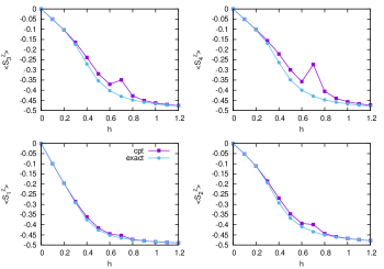
Figure 5: Magnetization of different sites versus magnetic field for a lattice of size $L=8$ with open boundary condition. The cluster size in CPT is $L_{c}=4$. Exact results are also reported for comparison

It is worth mentioning that the hard-core constraint implies the following relation between expectation values:

$$\langle a_{i}^{\dagger}a_{i}\rangle+\langle a_{i}a_{i}^{\dagger}\rangle=1\,.$$ (31)

We found that within the present self-consistent CPT the expectation value of the above expression slightly deviates from one by about $10^{-3}$ on the average, with a maximum of the order of $10^{-2}$ at $h=0.7$ and for the sites at the edge of the supercell, as shown by the kink around $h=0.7$ in Fig. 5. This is due to the fact that treating inter-cluster terms perturbatively violates the constraint within CPT, mainly for the edge sites.

V.2 Non-equilibrium results

In this section we present results for the real time dynamics of the Ising model within the variational cluster perturbation approach introduced above. To drive the system out of equilibrium we proceed as follows. We prepare the system at equilibrium for $t_{0}<0$ as the ground state of Eq. 4 with magnetic field $h_{0}$ and then we suddenly change the magnetic field to a different value $h$. As in equilibrium we use variational NE-CPT in a self-consistent way as described in section (IV). After finding the time dependent variational parameters for each time step in the mean-field approximation, we calculate Green’s function and condensate within CPT as described in Sec. IV.

To benchmark this idea for the non-equilibrium case we display in Fig. 6 the real time dynamics of magnetization for different sites on a lattice of size $L=8$ with open boundary condition at zero temperature. We compare results obtained exactly with results within CPT for a cluster size of $L_{c}=4$. We have reported the dynamics for the case of relatively large quench, from $h_{0}=0.2$ to $h=1.2$, for which the field crosses the phase transition. As we can see, NE-CPT provides quite good results for the magnetization compared to the exact one except for the edge sites where the hopping to the next supercell is treated perturbatively. At the beginning of the dynamics NE-CPT is very accurate and the deviation builds up as time progresses.

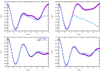
Figure 6: Time dependence of the magnetization in the $z$ direction for different sites on a lattice of size $L=8$. The cluster size in CPT is $L_{c}=4$. The magnetic field has been suddenly changed from $h_{0}=0.2$ to $h=1.2$. The exact dynamics is shown for comparison.

We have investigated different types of quenches and the behavior is qualitatively the same: the dynamics remains close to the exact one at short times and starts deviating at later times. As mentioned, the largest deviations are found at the edge sites.

In Fig. 7 we report NE-CPT results for the magnetization dynamics after the quench for an infinite lattice. We display results obtained for different cluster sizes and different types of quenches. For quenches into the ordered phase (see lower left and right panels), NE-CPT for a cluster of $L_{c}=6$ provides quite accurate results for the magnetization dynamics up to $t\approx 7$ (remember, that time is in unit of $1/J$). For a larger quench from $h_{0}=1.2$ to $h=0.4$, crossing the transition point, NE-CPT is able to reproduce the dynamics only up to a shorter value of the time $t\approx 5$ (see upper left panel). For quenches within the disordered phase (quench from $h_{0}=1.2$ to $h=1.6$) NE-CPT results show only a slight deviation ($\lesssim 10^{-3}$) from the exact one, however with some small oscillations (see upper right panel). Overall, NE-CPT results for an infinite system systematically improve by increasing cluster size $L_{c}$. Already for $L_{c}\approx 6$ they reproduce quite accurate results for the thermodynamic limit of a very long chain ($L=400$) up to $t\approx 7$.
Finally we report the real time quench dynamics of the magnetization for the two dimensional Ising Model, which is not exactly solvable. In $D=2$ the transverse field Ising model at zero temperature has an equilibrium phase transition at $h_{c}\approx 1.6$Friedman ; Elliott ; Oitmaa .

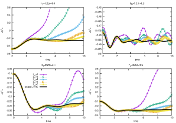
Figure 7: Time dependence of the magnetization for an infinite ising chain evaluated within NE-CPT with differnt cluster sizes $L_{c}$ compared with exact results for a chain of length $L=400$.

Within the self-consistent variational CPT at equilibrium we get instead $h_{c}\approx 1.9$, for the small $2\times 2$ clusters we are considering. We note that the accuracy of CPT improves systematically by increasing the cluster size. We show results for different types of quenches which are obtained either within a disordered or a ordered phase or a quench which crosses the critical field. Here we compare Lanczos exact results obtained for three different lattice sizes with periodic boundary condition to NE-CPT results using clusters of size $L_{c}=2\times 2$. We note that the largest size we can reach to perform real time quench dynamics within Lanczos at zero temperature is $L=4\times 4$.

For a small quench in the ordered phase, $h_{0}=0.2$ to $h=0.4$ (Fig. 8 lower left-panel) NE-CPT gives quite accurate results, as compared with Lanczos exact results. We observe that magnetization dynamics within NE-CPT is quite close to the best of the Lanczos for times up to $t_{max}=10$. We further note that in this case the Lanczos results already show convergence as a function of system size so that they can be considered as a good approximation to the thermodynamic limit for these values of the parameters. For a larger quench but still in the ordered phase, i.e. $h_{0}=1.2$ to $h=0.4$ (top left-panel of Fig. 8) the NE-CPT results compare well with Lanczos results up to $t_{max}\approx 6$. For quenches with large magnetic fields, i.e. into the disordered phase from $h_{0}=2.0$ to $h=2.5$ (top right-panel in Fig. 8) the Lanczos results have not converged yet, so a comparison is difficult to assess. Nevertheless, the NE-CPT results quantitatively agrees with the largest Lanczos system up to $t\approx 2$, and agrees qualitatively, i.e. displays similar oscillations, also for larger times. The lower right-panel in Fig. 8 shows the dynamics for a large magnetic quench that crosses the critical point, i.e. from $h_{0}=0.2$ to $h=2.0$. In this case the NE-CPT seems not to be accurate and is able to produce reliable dynamics only up to $t_{max}\approx 2$. We note that in all cases the magnetization stays within its physical values, $\left|S^{z}\right|\leq\frac{1}{2}$, except for a quench across the critical point. With cluster sizes of $L_{c}=2\times 2$ results are already promising in two dimensions, as long as one restricts to intermediate times. Furthermore, as in the $D=1$ case, NE-CPT results can be improved by systematically increasing the cluster size.

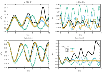
Figure 8: Dynamics for the magnetization compared to Lanczos results for different types of quenches in two dimension. NE-CPT calculation is for an infinite lattice with the cluster size of $L_{c}=2\times 2$.

VI Summary

We have introduced a variational formulatiuon of cluster perturbation theory (CPT) to investigate the quantum Ising model in and out of equilibrium at zero temperature. We find that plain CPT in equilibrium can describe accurately the system in the disordered phase, $h>h_{c}$, but looses accuracy while approaching the critical field $h_{c}$ and finally breaks down in the ordered phase, $h<h_{c}$. To describe the system in the broken symmetry region we developed a variational implementation of CPT, whereby an anomalous term is added to the cluster Hamiltonian and subtracted perturbatively. This parameter is then optimized within a self-consistent framework. We find a good agreement with exact results in the equilibrium case, for example concerning the magnetisation parallel to the magnetic field and the ground state energy.

Out of equilibrium the time dependent variational parameter are determined self-consistently for each time step. We find that this variational NE-CPT provides very accurate results for the short and intermediate time dynamics while getting inaccurate for longer times. Specifically in one dimension, comparing results of this NE-CPT approximation with exact calculations shows that clusters of size $L_{c}=6$ provide quite accurate description of the dynamics up to $t_{max}\approx 7$ for quenches within the ordered or disordered phases. When the critical point is crossed, the accuracy is limited to shorter times $t_{max}\approx 3$. A similar trend emerges also in two dimensions. Here, there is no exact solution to be compared with, so that we resort to finite-size Lanczos diagonalization to benchmark the method. One should notice, however, that NE-CPT can directly provide results in the thermodynamic limit. We highlight that the accuracy of NE-CPT can be systematically pushed to longer time by increasing the cluster size, at least up to the largest sizes still reachable by Lanczos time evolution.

This variational approach shall be considered as a first step to study hard-core bosons in and out of equilibrium by a variational CPT method. This idea could be improved and getting more elaborate by considering more variational terms and/or formulating it within the self-energy functional theoryHofmann .

VII Acknowledgment

We would like to thank M. Nuss, M. Aichhorn and A. Dorda for fruitful discussions. This work was supported by funds awarded by the Friuli Venezia Giulia autonomous Region Operational Program of the European Social Fund 2007/2013, Project DIANET-Danube Initiative and Alps Adriatic Network, CUP G93J12000220009. The work was also partially supported by the Austrian Science Fund (FWF): P26508, Y746, and NaWi Graz.

Appendix A Numerical solution of CPT equation

A.1 Time propagation

For spatially inhomogeneous systems, the computational limits are set by the memory requirement for saving big matrices in two time and spatial degrees of freedom. Considering $N_{K}$ time steps on the Keldysh and $N_{M}$ on the Matsubara for a lattice of size $L$ the required memory to save the Green’s function is

$$(2*L*(2*N_{K}+N_{M}))^{2}*16~{}~{}~{}bytes$$ (32)

Therefore, for a $N_{K}=1000,t_{max}=10$, $N_{M}=2000,\beta=10$, $L=8$ the required memory is $61$ Gigabytes. This example shows that reaching large time or large system sizes ($t\gtrsim 10J,L\gtrsim 6$) is prohibitive since the memory requirement is beyond the capabilities of standard available computational resources. Another issue is the inversion of the huge matrix in the CPT equation to get the lattice Green’s function. When the matrix size increases the inversion process takes longer time and also the numerical error will increase.
Based on the above facts one has to design a way to avoid matrix inversion and the storage of huge matrices to finally be able to reach longer times for the dynamics of the system.

A.2 Procedure to propagate the CPT equation in time

In this section, we summarize the procedure to numerically solve the CPT equation by gradually progressing in time in order to avoid inversion and storage of big matrices. Since this equation is of the Kadanoff-Baym type, there is a great deal of literature on the subject (see, e.g. Bonitz ). For example, the method is used in time dependent dynamical mean-field theory (TDMFT) Aoki ; Tran , where, however the system is typically translationally invariant. In our case, where we deal with finite systems, we have to consider spatial degrees of freedom and, accordingly, solve a corresponding set of equations for inhomogeneous system.

Here, we roughly follow the treatment of Ref. Tran , see also  Bonitz . Here, in addition, we consider the case of an inhomogenous system. The CPT equation for the Green’s function $\hat{G}$ of the physical system is

$$\hat{G}=\hat{G_{0}}+\hat{G_{0}}\bullet\hat{V}\bullet\hat{G}$$ (33)

Where $\hat{G_{0}}$ is the cluster Green’s function and $\hat{V}=V\bigotimes\mathbb{1}$ is the inter-cluster term. By introducing $\hat{K}=\hat{G_{0}}\bullet\hat{V}$ we rewrite the CPT equation as

$$\hat{G}=\hat{G_{0}}+\hat{K}\bullet\hat{G}$$ (34)

and after writing the contour integration explicitly we have

$$\hat{G}(z,z^{\prime})=\hat{G}_{0}(z,z^{\prime})+\int_{\cal{C}}dz_{1}\hat{K}(z,z_{1})\hat{G}(z_{1},z^{\prime})$$ (35)

Using Langreth theorem Langreth we can write the integral equation for the components of the Green’s function on the contour. We obtain the following equations:

$$\begin{split}G^{<}=G_{0}^{<}+K^{<}\cdot G^{A}+K^{R}\cdot G^{<}+K^{\rceil}*G^{\lceil}\\ G^{>}=G_{0}^{>}+K^{>}\cdot G^{A}+K^{R}\cdot G^{>}+K^{\rceil}*G^{\lceil}\\ G^{R}=G_{0}^{R}+K^{R}\cdot G^{R}\\ G^{A}=G_{0}^{A}+K^{A}\cdot G^{A}\\ G^{\rceil}=G_{0}+K^{R}\cdot G^{\rceil}+K^{\rceil}*G^{M}\\ G^{\lceil}=G_{0}^{\lceil}+K^{\lceil}\cdot G^{A}+K^{M}*G^{\lceil}\\ G^{M}=G_{0}^{M}+K^{M}*G^{M}\end{split}$$ (36)

where . means integration over real time and $*$ over imaginary time (Matsubara branch).
We are interested in the magnetization which can be calculated from the lesser ($G^{<}$) Green’s function. To Solve the equation for $G^{<}$ first we need to calculate $G^{A}$ and $G^{\lceil}$ within CPT. Furthermore to determine $G^{\lceil}$ we need to evaluate the Matsubara Green’s function $G^{M}$ which can be calculated with equilibrium techniques. The cluster Green’s function $G_{0}^{\alpha}$, ($\alpha=<,R,A,>,\lceil,\rceil$) also should be calculated for an affordable cluster size.
It is also worth to mention that due to the presence of anomalous terms like $a_{i}a_{j}$ and $a_{i}^{\dagger}a_{j}^{\dagger}$ in the Hamiltonian of Eq. (6) the structure of the Green’s function matrix also should include anomalous Green’s functions in order to satisfy the correct equation of motion. Therefore the $G^{\alpha}$, ($\alpha=<,R,A,>,\lceil,\rceil$), is a matrix in itself with the following Nambu structure

$$G^{\alpha}=\begin{bmatrix}g^{\alpha}&f^{\alpha}\\ f^{\alpha{\dagger}}&k^{\alpha}\end{bmatrix}$$ (37)

The definition of the Green’s functions are as follow:
1) Advanced Green function:

$$\begin{split}g_{i,j}^{A}(t,t^{\prime})=i\theta(t^{\prime}-t)[\langle a_{i}(t)a_{j}^{\dagger}(t^{\prime})\rangle-\langle a_{j}^{\dagger}(t^{\prime})a_{i}(t)\rangle]\\ k_{i,j}^{A}(t,t^{\prime})=i\theta(t^{\prime}-t)[\langle a_{i}^{\dagger}(t)a_{j}(t^{\prime})\rangle-\langle a_{j}(t^{\prime})a_{i}^{\dagger}(t)\rangle]\\ f_{i,j}^{A}(t,t^{\prime})=i\theta(t^{\prime}-t)[\langle a_{i}(t)a_{j}(t^{\prime})\rangle-\langle a_{j}(t^{\prime})a_{i}(t)\rangle]\\ f_{i,j}^{{\dagger}A}(t,t^{\prime})=i\theta(t^{\prime}-t)[\langle a_{i}^{\dagger}(t)a_{j}^{\dagger}(t^{\prime})\rangle-\langle a_{j}^{\dagger}(t^{\prime})a_{i}^{\dagger}(t)\rangle]\\ \end{split}$$ (38)

2) Retarded Green’s function:

$$\begin{split}g_{i,j}^{R}(t,t^{\prime})=-i\theta(t-t^{\prime})[\langle a_{i}(t)a_{j}^{\dagger}(t^{\prime})\rangle-\langle a_{j}^{\dagger}(t^{\prime})a_{i}(t)\rangle]\\ k_{i,j}^{R}(t,t^{\prime})=-i\theta(t-t^{\prime})[\langle a_{i}^{\dagger}(t)a_{j}(t^{\prime})\rangle-\langle a_{j}(t^{\prime})a_{i}^{\dagger}(t)\rangle]\\ f_{i,j}^{R}(t,t^{\prime})=-i\theta(t-t^{\prime})[\langle a_{i}(t)a_{j}(t^{\prime})\rangle-\langle a_{j}(t^{\prime})a_{i}(t)\rangle]\\ f_{i,j}^{{\dagger}R}(t,t^{\prime})=-i\theta(t-t^{\prime})[\langle a_{i}^{\dagger}(t)a_{j}^{\dagger}(t^{\prime})\rangle-\langle a_{j}^{\dagger}(t^{\prime})a_{i}^{\dagger}(t)\rangle]\\ \end{split}$$ (39)

There is relation between retarded and advanced green’s function: $G^{R}(t,t^{\prime})=G^{A{\dagger}}(t^{\prime},t)$.
3) Lesser Green’s function

$$\begin{split}g_{i,j}^{<}(t,t^{\prime})=-i\langle c_{j}(t^{\prime})^{\dagger}c_{i}(t)\rangle\\ f_{i,j}^{<}(t,t^{\prime})=-i\langle c_{j}(t^{\prime})c_{i}(t)\rangle\\ f_{i,j}^{<{\dagger}}(t,t^{\prime})=-i\langle c_{j}(t^{\prime})^{\dagger}c_{i}(t)^{\dagger}\rangle\\ k_{i,j}^{<}(t,t^{\prime})=-i\langle c_{j}(t^{\prime})c_{i}(t)^{\dagger}\rangle\end{split}$$ (40)

4) Mixing Green’s function:

$$\begin{split}g^{\lceil}_{i,j}(\tau,t)=-i\langle c_{i}(\tau)c_{j}^{\dagger}(t)\rangle\\ f^{\lceil}_{i,j}(\tau,t)=-i\langle c_{i}(\tau)c_{j}(t)\rangle\\ f^{\lceil{\dagger}}_{i,j}(\tau,t)=-i\langle c_{i}^{\dagger}(\tau)c_{j}^{\dagger}(t)\rangle\\ k^{\lceil}_{i,j}(\tau,t)=-i\langle c_{i}^{\dagger}(\tau)c_{j}(t)\rangle\\ g^{\rceil}_{i,j}(t,\tau)=-i\langle c_{j}(\tau)^{\dagger}c_{i}(t)\rangle\\ f^{\rceil}_{i,j}(t,\tau)=-i\langle c_{j}(\tau)c_{i}(t)\rangle\\ f^{\rceil{\dagger}}_{i,j}(t,\tau)=-i\langle c_{j}(\tau)^{\dagger}c_{i}(t)^{\dagger}\rangle\\ k^{\rceil}_{i,j}(t,\tau)=-i\langle c_{j}(\tau)c_{i}(t)^{\dagger}\rangle\\ \end{split}$$ (41)

If we write the integral equation for $G^{A}$ we get (omitting the spatial indexes):

$$\begin{split}G^{A}(t,t^{\prime})=G_{0}^{A}(t,t^{\prime})+\int K^{A}(t,\bar{t})G^{A}(\bar{t},t^{\prime})d\bar{t}\\ G^{A}(t,t^{\prime})=G_{0}^{A}(t,t^{\prime})+\int_{t}^{t^{\prime}}K^{A}(t,\bar{t})G^{A}(\bar{t},t^{\prime})d\bar{t}\\ \end{split}$$ (42)

To perform the integration, we discretize the time with equal spacing

$$\begin{split}t_{i}=i\times\Delta t+t_{0},~{}~{}\Delta t=\frac{t_{max}-t_{0}}{N_{K}-1},~{}~{}(i=0,1,...,N_{K}-1)\\ \tau_{i}=i\times\Delta\tau+t_{0},~{}~{}\Delta\tau=\frac{-i\beta-t_{0}}{N_{M}-1},~{}~{}(i=0,1,...,N_{M}-1)\end{split}$$ (43)

where $N_{K}$ and $N_{M}$ are the number of time points on the real and imaginary branch respectively. After approximating the integral by the trapezoid rule

$$\begin{split}\int_{t_{a}}^{t_{b}}f(x)dx\approx\Delta t\sum_{i=0}^{N-1}\omega_{i}f(x_{i}),~{}~{}~{}\Delta t=\frac{t_{b}-t_{a}}{N-1}\\ w_{i}=\left\{\begin{array}[]{cc}1/2&i=0,N-1\\ 1&1\leq i\leq N-2\end{array}\right.\end{split}$$ (44)

we get

$$\begin{split}G^{A}(t_{m},t^{\prime}_{n})\approx G_{0}^{A}(t_{m},t^{\prime}_{n})+\Delta\bar{t}\sum_{i=m}^{n}w_{i}K^{A}(t_{m},\bar{t_{i}})G^{A}(\bar{t_{i}},t^{\prime}_{n})\\ G^{A}(t_{m},t^{\prime}_{n})\approx G_{0}^{A}(t_{m},t^{\prime}_{n})+\Delta\bar{t}\sum_{i=m+1}^{n}w_{i}K^{A}(t_{m},\bar{t_{i}})G^{A}(\bar{t_{i}},t^{\prime}_{n})\\ \end{split}$$ (45)

where $K^{A}(t_{m},t_{m})=0$ is used. In the equation for $G^{A}$ it is not possible to gradually propagate in the direction of time since $G^{A}(t_{m},*)$ depends on later times $m+1,...n$, in other words this equation is not of the Volterra type Brunner where the causal structure is evident from the limits of the integral. To get a Volterra type of equation for the $G^{A}$ we have to use another form of the CPT equation:

$$\hat{G}=\hat{G_{0}}+\hat{G}\bullet\hat{V}\bullet\hat{G_{0}}$$ (46)

where now $\hat{K}=\hat{V}\bullet\hat{G_{0}}$. Proceeding in the same way as above we derive the following equation in discretized time for the advanced Green’s function

$$\boxed{G^{A}(t_{m},t^{\prime}_{n})\approx G_{0}^{A}(t_{m},t^{\prime}_{n})+\Delta\bar{t}\sum_{i=m+1}^{n-1}w_{i}G^{A}(t_{m},\bar{t_{i}})K^{A}(\bar{t_{i}},t^{\prime}_{n})}$$ (47)

We now can gradually proceed in the second index $t^{\prime}_{n}$ for a fixed $t_{m}$.
Similarly for the retarded Green’s function we get

$$\boxed{\begin{split}G^{R}(t_{m1},t^{\prime}_{m2})\approx G_{0}^{A}(t_{m1},t^{\prime}_{m2})+\\ \Delta\bar{t}\sum_{i=m2+1}^{m1-1}w_{i}K^{R}(t_{m1},\bar{t_{i}})G^{R}(\bar{t_{i}},t^{\prime}_{m2})\end{split}}$$ (48)

where we can progress in time by incrementing $t_{m1}$ for a fixed $t^{\prime}_{m2}$.
For the mixed Green’s function if we use the CPT Eq. (46) we obtain the following integral equation:

$$\begin{split}G^{\lceil}(\tau,t)\approx G_{0}^{\lceil}(\tau,t)+\int_{0}^{t^{\prime}}K^{\lceil}(\tau,\bar{t})G^{A}(\bar{t},t)d\bar{t}+\\ \int_{0}^{-i\beta}K^{M}(\tau,\bar{\tau})G^{\lceil}(\bar{\tau},t)d\bar{\tau}\end{split}$$ (49)

Since in the convolution including $G^{\lceil}$ the integration over $\tau$ is on the whole Matsubara branch, it is not possible to gradually proceed in time. So the way out is to choose the other CPT Eq. (46) to end up in a Volterra type equation

$$\boxed{\begin{split}G^{\lceil}(\tau_{m1},t_{m2})\approx G_{0}^{\lceil}(\tau_{m1},t_{m2})+\\ \Delta t\sum_{i=0}^{m2-1}w_{i}G^{\lceil}(\tau_{m1},t_{i})K^{A}(t_{i},t_{m2})\\ +\Delta\tau\sum_{i=0}^{N_{M}-1}w_{i}G^{M}(\tau_{m1},\tau_{i})K^{\lceil}(\tau_{i},t_{m2})\;.\end{split}}$$ (50)

Here one can proceed in $t_{m2}$ for a fixed $\tau_{m1}$. The full information of the Matsubara Green’s function on the imaginary axis is necessary to calculate the mixing Green’s function. This can be done by equilibrium techniques, see appendix B.
Finally for the lesser greens function we have:

$$\boxed{\begin{split}G^{<}(t_{m1},t_{m2})\approx G_{0}^{<}(t_{m1},t_{m2})+\\ \Delta t\sum_{i=0}^{m2-1}w_{i}K^{<}(t_{m1},t_{i})G^{A}(t_{i},t_{m2})\\ +\Delta\tau\sum_{i=0}^{N_{M}-1}w_{i}K^{\rceil}(t_{m1},\tau_{i})G^{\lceil}(\tau_{i},t_{m2})\\ +\Delta t\sum_{i=0}^{m1-1}w_{i}K^{R}(t_{m1},t_{i})G^{<}(t_{i},t_{m2})\end{split}}$$ (51)

Appendix B Calculating equilibrium Green’s function $G^{M}$

The CPT equation for $G^{M}$ is not of the Volterra type, so it is not possible to gradually proceed along the Matsubara axes. Fortunately due to the time translation invariance of the Green’s function, $G^{M}$ only depend on the time difference and so one can use Fourier transformation to go over to the frequency representation. In this way one still has to do inversion process to get CPT Green’s function but in this way the dimension reduces to the size of the lattice.
The Fourier transformations between the Green’s functions are as follow:

$$\begin{split}G(\tau)=\frac{1}{\beta}\sum_{n=-\infty}^{\infty}G(i\omega_{n})e^{-i\omega_{n}\tau}\\ G(i\omega_{n})=\int_{0}^{\beta}d\tau e^{i\omega_{n}\tau}G(\tau)\end{split}$$ (52)

where $\tau\in[0,\beta]$. By using fast Fourier transformation (FFTW) the above transformation can be carried out efficiently. When doing the inverse transformation we truncate the number of Matsubara frequencies. Using $N$ points equally distributed among positive and negative frequencies we get the approximation

$$\begin{split}G(\tau)\approx\frac{1}{\beta}\sum_{n=-N/2}^{N/2-1}G(i\omega_{n})e^{-i\omega_{n}\tau}=DIFT[G(i\omega_{n})]\\ \omega_{n}=\frac{\pi}{\beta}2n\end{split}$$ (53)

This scheme poorly describes $G(\tau)$ due to missing contributions from the tail of $G(\i\omega)$ ($\omega_{n}\to\infty$). In practice, it is not possible to consider an infinite number of frequencies so one should calculate the tail correction directly. If we look at the asymptotic behavior ($\omega_{n}\to\infty$) for the non-interacting Green’s function we realize

$$G(i\omega_{n})\sim-\frac{i}{\omega_{n}}$$ (54)

The asymptotic tail of $G_{A}(\tau)$ can be readily calculated by doing the Fourier transformation. For bosons we get:

$$G_{A}(\tau)=-\frac{2}{\beta}\sum_{n=0}^{\infty}\frac{\sin(\omega_{n}\tau)}{\omega_{n}}=-\frac{1}{2}+\frac{\tau}{\beta}$$ (55)

After a little algebra we can collect all contributions at high imaginary frequencies in the tail of the Green’s function $G_{T}(\tau)$ and write:

$$\begin{split}G(\tau)=DIFT[G(i\omega_{n})]+G_{T}(\tau)\\ G_{T}(\tau)=-\frac{1}{2}+\frac{\tau}{\beta}+\frac{2\pi}{\beta}\sum_{n=0}^{N/2-1}\frac{\sin(\omega_{n}\tau)}{\omega_{n}}\end{split}$$ (56)

References

- (1) I. Bloch, J. Dalibard, and W. Zwerger, Rev. Mod. Phys. 80, 885 (2008)
- (2) M. Lewenstein, A. Sanpera, and V. Ahufinger, Ultracold Atoms in Optical Lattices Simulating quantum many-body systems, Oxford University Press, Oxford (2012)
- (3) N. Strohmaier, D. Greif, R. Jördens, L. Tarruell, H. Moritz, and T. Esslinger, Phys. Rev. Lett. 104, 080401 (2010)
- (4) Sachdev, Subir, Quantum Phase Transitions, Cambridge: Cambridge University Press (1999)
- (5) S. Suzuki, J-i Inoue and Bikas K. Chkarabarti, Quantum Ising Phases and Transitions in Transverse Ising Models, Springer, Lecture Notes in Physics, Vol. 862 (2013)
- (6) F. Meinert, M. J. Mark, E. Kirilov, K. Lauber, P. Weinmann, A. J. Daley, and H.-C. N¨agerl, Phys. Rev. Lett. 111, 053003 (2013)
- (7) D. Rossini, A. Silva, G. Mussardo, and G. E. Santoro, Phys. Rev. Lett. 102, 127204 (2009)
- (8) P. Calabrese, F. H. L. Essler, and M. Fagotti, Phys. Rev. Lett. 106 , 227203 (2011)
- (9) R. Kubo, J. Phys. Soc. Jpn. 12, 570 (1957)
- (10) J. Schwinger, J. Math. Phys. 2, 407 (1961)
- (11) L. P. Kadanoff and G. Baym, Quantum Statistical Mechanics (Benjamin, New York, 1962)
- (12) L. V. Keldysh, Sov. Phys. JETP 20, 1018 (1965)
- (13) M. Wagner, Phys. Rev. B44, 6104 (1991)
- (14) J. K. Freericks, V. M. Turkowski, and V. Zlatic, Phys. Rev. Lett. 97, 266408 (2006)
- (15) P. Schmidt and H. Monien, preprint arXiv:cond-mat 0202046 (2002)
- (16) F. Hofmann, M. Eckstein, E. Arrigoni, and M. Potthoff, Phys. Rev. B88, 165124 (2013)
- (17) C. Jung, A. Lieder, S. Brener, H. Hafermann, B. Baxevanis, A. Chudnovskiy, A. N. Rubtsov, M. I. Katsnelson, and A. I. Lichtenstein, arXiv: 1011.3264 (2010)
- (18) M. Knap, W. von der Linden and E. Arrigoni, and Phys. Rev. B84, 115145 (2011)
- (19) H. Aoki and N. Tsuji, Rev. Mod. Phys. 86, 779 (2014)
- (20) K. Balzer, and M. Eckstein, Phys. Rev. B89, 035148 (2014)
- (21) M. Balzer, and M. Potthof, Phys. Rev. B83, 195132 (2011)
- (22) C. Gramsch, and M. Potthoff, Phys. Rev. B92, 235135 (2015)
- (23) E. Arrigoni, M. Knap, and W. von der Linden, Phys. Rev. Lett. 110, 086403 (2013)
- (24) A. Dorda, M. Nuss, W. von der Linden, and E. Arrigoni, Phys. Rev. B89, 165105 (2014)
- (25) A. Dorda, M. Ganahl, H. G. Evertz, W. von der Linden, and E. Arrigoni, Phys. Rev. B92, 125145 (2015)
- (26) D.D. Sénéchal, D. Perez, and M. Pioro-Ladrière Phys. Rev. Lett. 84, 522 (2000)
- (27) D.D. Sénéchal, D. Perez, and D. Plouffe Phys. Rev. B66, 075129 (2002)
- (28) W. Metzner, Phys. Rev. B43, 8549 (1991)
- (29) S. Pairlaut, D. Sénéchal, and A. M. S. Tremblay Euro. Phys. J. B 16, 85 (2000)
- (30) H. Hafermann, S. Brener, A. N. Rubstov, M. I. Katsnelson, and A. I. Lichtenstein, JETP Lett. 86, 677 (2007)
- (31) C. Gros and R. Valentí Phys. Rev. B48, 418 (1993)
- (32) M. Bonitz, Progress in Nonequilibrium Green’s functions IV, World Scientific, Singapore (2000)
- (33) E. Arrigoni, M. Knap, and W. von der Linden, Phys. Rev. B84, 014535 (2011)
- (34) M. T. Tran, Phys. Rev. B78, 125103 (2008)
- (35) E. Lieb, T. Schultz, and D. Mattis, Ann. Phys (Berlin) 16, 407 (1961)
- (36) P. Pfeuty, Ann. Phys (Berlin) 57, 79 (1970)
- (37) O. Derzhko, Journal of Physical Studies (L’viv), 5, 49 (2001)
- (38) P. Danielewicz, Ann. Phys. (N.Y) 152, 239 (1984)
- (39) J. Rammer and H. Smith, Rev. Mod. Phys. 58, 323 (1986)
- (40) M. Potthoff, Eur. Phys. J. B. 32, 429 (2003)
- (41) M. Potthoff, Eur. Phys. J. B. 36, 335 (2003)
- (42) W. Koller and N. Dupuis, J. Phys: Condens. Matter 18, 9525 (2006).
- (43) M. Aichhorn, E. Arrigoni, M. Potthoff, and W. Hanke Phys. Rev. B74, 235117 (2006)
- (44) M. G. Zacher, R. Eder, E. Arrigoni, and W. Hanke Phys. Rev. B65, 045109 (2002)
- (45) M. Knap, E. Arrigoni, and W. von der Linden Phys. Rev. B81, 024301 (2010)
- (46) M. Knap, E. Arrigoni, and W. von der Linden Phys. Rev. B83, 134507 (2011)
- (47) Z. Friedman, Phys. Rev. B17, 1429 (1978)
- (48) R. J. Elliott and C. Wood, J. Phys. C 4, 2359 (1971)
- (49) J. Oitmaa and M. Plischke, J. Phys. C 9, 2093 (1976)
- (50) D. C. Langreth, Linear and Nonlinear Electron Transport in Solids (Plenum Press, New York and London), edited by J. T. Devreese and V. E.. van Doren (1976)
- (51) H. Brunner, and P. J. van der Houwen, The Numerical Solution of Volterra Equations (North-Holland, Amsterdam) 1986